Multi-branched resonances, chaos through quasiperiodicity, and asymmetric states in a superconducting dimer

Abstract

A system of two identical SQUIDs (superconducting quantum interference devices) symmetrically coupled through their mutual inductance and driven by a sinusoidal field is investigated numerically with respect to dynamical properties such as its multibranched resonance curve, its bifurcation structure, as well as its synchronization behavior. The SQUID dimer is found to exhibit a hysteretic resonance curve with a bubble connected to it through Neimark-Sacker (torus) bifurcations, along with coexisting chaotic branches in their vicinity. Interestingly, the transition of the SQUID dimer to chaos occurs through a period-doubling cascade of a two-dimensional torus (quasiperiodicity-to-chaos transition). The chaotic states are identified through the calculated Lyapunov spectrum, and their basins of attraction have been determined. Bifurcation diagrams have been constructed on the parameter plane of the coupling strength and the driving frequency of the applied field, and they are superposed to maps of the maximum Lyapunov exponent on the same plane. In this way, a clear connection between chaotic behavior and torus bifurcations is revealed. Moreover, asymmetric states that resemble localized synchronization have been detected using the correlation function between the fluxes threading the loop of the SQUIDs. The effect of intermittent chaotic synchronization, which seems to be present in the SQUID dimer, is only slightly touched.

Networks of coupled limit cycle oscillators represent a class of systems with special interest in physics, chemistry, and biological sciences. Arrays of coupled nonlinear oscillators, in particular, which often exhibit complex dynamical behavior, have attracted large amounts of theoretical, numerical, and experimental efforts. However, the prominent features of a finite large number of such oscillators can be sometimes understood by analysing just two coupled oscillators. A unique in many aspects oscillator is the superconducting quantum interference device (SQUID) that has been investigated extensively for many years. The SQUID is a low-loss, highly nonlinear resonant element that responds strongly to applied magnetic field(s) and exhibits rich dynamical behavior. Moreover, it has recently been the elementary unit for the construction of metamaterials in one and two dimensions. SQUIDs and SQUID arrays are technologically important devices, and they also serve as a testbed for exploring complex dynamics. Two SQUIDs in close proximity are coupled together through magnetic dipole-dipole forces, and their dynamical complexity significantly increases. Specifically, more complex bifurcation scenarios appear, along with transitions to chaos through quasiperiodicity, the emergence of localized synchronization, and intermittent chaotic synchronization. These dynamical properties are explored numerically with a well-established model whose parameters are acquired from recent relevant experiments.

I Introduction

There has been great interest on the behavior of systems with interacting and forced nonlinear oscillations with applications in physics, biology, and chemistry, which in addition are in abundance in the natural world Awrejcewicz1991 . The interaction introduces qualitatively new behavior to the network of oscillators, as compared to that of a single oscillator. For example, synchronization of the oscillating units of the system Rosenblum2003 , extreme multistability Wiesenfeld1989 ; Nishio1992 , multiple resonance and anti-resonance effects Jothimurugan2016 ; Kominis2019 ; Sarkar2019 , complex bifurcation structure Yin1998 ; Kenfack2003 , localization Lazarides2010 , emergence of exceptional points Kominis2018 , the intriguing effect of amplitude death Herrero2000 , chaos synchronization Tafo2009 , localized synchronization Hohl1997 , chaos to hyperchaos transitions Kapitaniak1991 ; Kapitaniak1995 ; Kapitaniak2000 ; Grygiel2000 , and quasi-periodicity with subsequent transition to chaos Rand1982 ; Bishop1986 ; Kozlowski1995 ; Dixon1996 ; Elhadj2008 ; Borkowski2015 , are some of the experimentally or numerically observed behaviors.

Here we consider a pair of coupled nonlinear oscillators (i.e., a nonlinear dimer) that belong to the large class of externally driven and dissipative systems. More specifically, we consider a pair of identical mutually coupled SQUID oscillators Kleiner2004 ; Fagaly2006 , where the acronym stands for “superconducting quantum interference device”. SQUIDs are mesoscopic superconducting devices which are modeled efficiently by equivalent electrical circuits, while their dynamics is governed by a second order nonlinear ordinary differential equation. The simplest variant of a SQUID consists of a superconducting loop interrupted by a Josephson junction (JJ), called rf SQUID, which was found to exhibit very rich dynamic behavior, including complex bifurcation structure and chaos Hizanidis2018 . Moreover, rf SQUIDs are employed as elementary units for the fabrication of superconducting metamaterials, whose investigation has revealed several extraordinary properties Trepanier2013 ; Zhang2015 . Recent theoretical works on SQUID metamaterials have also reported the existence of chimera states and pattern formation LAZ15 ; HIZ16a ; HIZ16b ; HIZ20 .

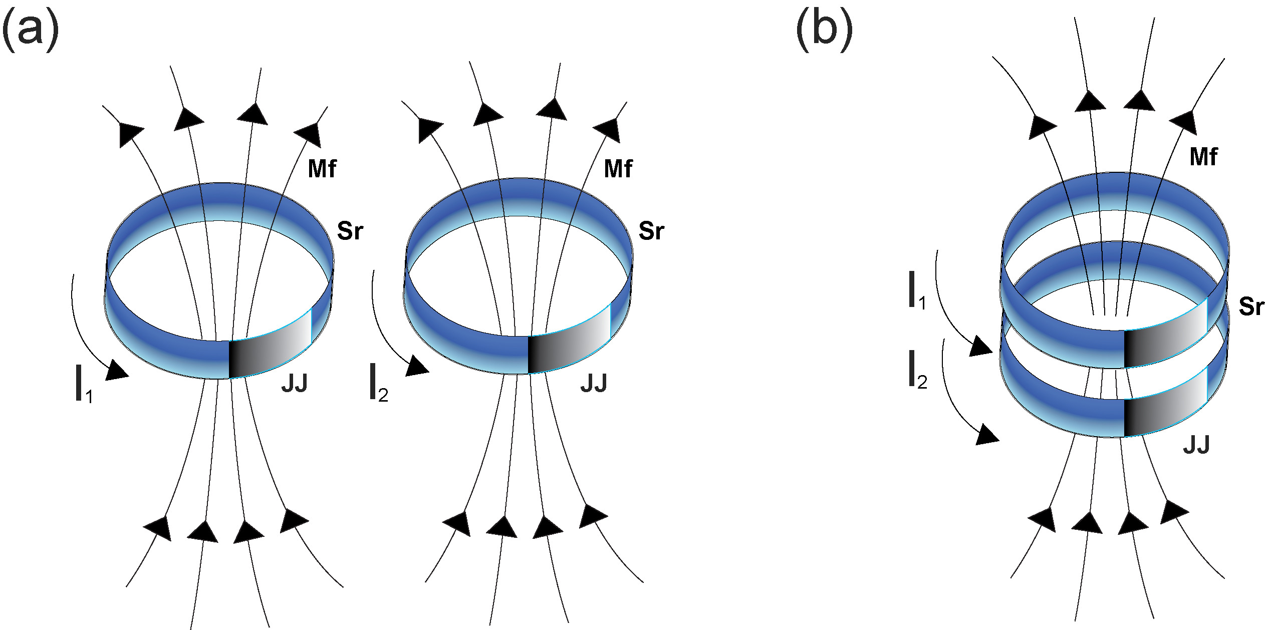
Figure 1: Schematic diagram of a SQUID dimer in a magnetic field where “Mf” is the Magnetic field, “Sr” is the Superconducting ring, “JJ” is the Josephson Junction, and $I_{1}$, $I_{2}$ are the induced currents. Panels (a) and (b) correspond to negative and positive magnetic coupling strength, respectively, appropriate for the planar and the axial geometry.

Two SQUIDs in relatively close proximity are coupled together by magnetic dipole-dipole forces due to their mutual inductance $\cal M$, while the sign and the magnitude of their coupling strength coefficient depends strongly on their relative positions. Specifically, the two SQUIDs may be arranged either in the planar geometry (Fig. 1(a)), where they lie in the same plane with their axes in parallel, or in the axial geometry, they lie the one on top of the other with their axes lying on the same line (Fig. 1(b)). The SQUIDs are driven by externally applied periodic and constant (bias) magnetic fields of appropriate polarization, to which they respond resonantly. Although its potential for technological applications, the dynamics of a SQUID dimer are not properly investigated. Recently however, the existence of homoclinic chaos in a pair of parametrically driven SQUIDs has been exposed Agaoglou2015 ; Agaoglou2017 .

In the present work, particular dynamical properties of a SQUID dimer are addressed, such as its highly unusual resonance curve that consists of a bistable part with a bubble connected to it through Neimark-Sacker (NS) and pitchfork bifurcations (PBs). These bubbles are of very different character compared to those reported long ago by Bier and Bountis BIE84 and they deserve to be investigated on their own. Moreover, in addition to those solutions, there are at least two more coexisting solutions in the frequency interval spanned by the resonance curve, which end up becoming chaotic through quasiperiodicity, i.e., through period doubling bifurcations of two-dimensional (2D) tori. The basins of attraction leading to chaos are calculated for two parameter sets of particular importance. Furthermore, asymmetric solutions either synchronized (leading to localized synchronization) or anti-synchronized (i.e., having opposite phases) are investigated by calculating the maximum Lyapunov exponent and the correlation function over the entire control parameter space.

In the next section (II), the electrical circuit equivalent model for the SQUID dimer is described in detail, and the dynamic equations are obtained. In section III, the bifurcation structure for the SQUID dimer is discussed along with the emergence of quasiperiodicity and chaos. Section IV is devoted to the transition to chaos through quasiperiodicity, through a Neimark-Sacker (NS) bifurcation. The existence of highly asymmetric solutions related to localized synchronization is revealed using an appropriate correlation function in section V. Conclusions are given in section VI.

II Modeling Two Coupled SQUIDs

Consider two identical rf SQUIDs in close proximity so that they are coupled by magnetic dipole-dipole forces through their mutual inductance $\cal M$ (Fig. 1). Each of the SQUIDs is modeled by an equivalent electrical circuit that features a self-inductance $L$ due to the superconducting ring, which is connected in series with a “real” Josephson junction Josephson1962 characterized by a critical current $I_{c}$, capacitance $C$, and Ohmic resistance $R$ Hizanidis2018 . The SQUIDs are subject to an externally applied spatially constant and time-periodic (ac) magnetic field and a constant in time and space (dc) magnetic field. Those fields add an electromotive force in series to the SQUID’s equivalent circuits. The magnetic flux threading the loops of the SQUIDs includes supercurrents as well as normal (i.e., quasiparticle) currents around the SQUID’s rings through Faraday’s law. In turn, the induced currents produce their own magnetics field which counter-acts the applied ones. Then, the flux $\Phi_{1}$ and $\Phi_{2}$ through the loop of the SQUID number $1$ and $2$, respectively, is given by the following flux-balance relations

$$\Phi_{1}=\Phi_{ext}+L\,I_{1}+{\cal M}I_{2},$$ (1)

$$\Phi_{2}=\Phi_{ext}+L\,I_{2}+{\cal M}I_{1},$$ (2)

where $I_{1}$ and $I_{2}$ are the currents induced by the external magnetic fields, and the external flux

$$\Phi_{ext}=\Phi_{dc}+\Phi_{ac}\,\cos(\omega t),$$ (3)

with $\Phi_{dc}$ the dc flux bias, $\Phi_{ac}$ the amplitude of the ac flux, $\omega$ its frequency, and $t$ the temporal variable. Eqs. (1) and (2) can be solved for the currents and written in matrix form as

$$\begin{bmatrix}I_{1}\\ I_{2}\end{bmatrix}=\frac{1}{L}\begin{bmatrix}1&\lambda\\ \lambda&1\end{bmatrix}^{-1}\begin{bmatrix}\Phi_{1}-\Phi_{ext}\\ \Phi_{2}-\Phi_{ext}\end{bmatrix},$$ (4)

where $\lambda=\frac{\cal M}{L}$ is the magnetic coupling strength between the SQUIDs. Note that the sign of $\lambda$ depends on the mutual position of the two SQUIDs. In the planar geometry (Fig. 1(a)), that sign is negative, while in the axial geometry (Fig. 1(b)), it is positive. The currents flowing in the SQUIDs are given within the framework of the resistively and capacitively shunted junction (RCSJ) model Likharev1986 , as

$$I_{n}=-C\frac{d^{2}\Phi_{n}}{dt^{2}}-\frac{1}{R}\frac{d\Phi_{n}}{dt}-I_{c}\,\sin\left(2\pi\frac{\Phi_{n}}{\Phi_{0}}\right),$$ (5)

where $\Phi_{0}$ is the flux quantum, and $n=1,2$. Combining Eqs. (4) and (5) we get the coupled equations for the fluxes through the loops of the SQUIDs in natural units, as

$$L\,C\frac{d^{2}\Phi_{1}}{dt^{2}}+\frac{L}{R}\frac{d\Phi_{1}}{dt}+L\,I_{c}\,\sin\left(2\pi\frac{\Phi_{1}}{\Phi_{0}}\right)+\frac{1}{1-\lambda^{2}}\Phi_{1}$$

$$-\frac{\lambda}{1-\lambda^{2}}\Phi_{2}=\frac{1}{1+\lambda}\Phi_{ext},$$ (6)

$$L\,C\frac{d^{2}\Phi_{2}}{dt^{2}}+\frac{L}{R}\frac{d\Phi_{2}}{dt}+L\,I_{c}\,\sin\left(2\pi\frac{\Phi_{2}}{\Phi_{0}}\right)+\frac{1}{1-\lambda^{2}}\Phi_{2}$$

$$-\frac{\lambda}{1-\lambda^{2}}\Phi_{2}=\frac{1}{1+\lambda}\Phi_{ext},$$ (7)

In normalized form, Eqs. (II) and (II) can be written as

$$\ddot{\phi_{1}}+\gamma\dot{\phi_{1}}+\beta\,\sin\left(2\pi\phi_{1}\right)+\frac{1}{1-\lambda^{2}}\phi_{1}-\frac{\lambda}{1-\lambda^{2}}\phi_{2}$$

$$=\frac{1}{1+\lambda}\phi_{ext},$$ (8)

$$\ddot{\phi_{2}}+\gamma\dot{\phi_{2}}+\beta\,\sin\left(2\pi\phi_{2}\right)+\frac{1}{1-\lambda^{2}}\phi_{2}-\frac{\lambda}{1-\lambda^{2}}\phi_{1}$$

$$=\frac{1}{1+\lambda}\phi_{ext},$$ (9)

with

$$\phi_{ext}=\phi_{dc}+\phi_{ac}\,\cos\left(\Omega\tau\right),$$ (10)

where all the fluxes $\Phi_{1},\Phi_{2},\Phi_{ac},\Phi_{dc}$ are in units of the flux quantum $\Phi_{0}$ and the new temporal variable $\tau$ is defined as $\tau=t\,\omega_{LC}$ with $\omega_{LC}=1/\sqrt{L\,C}$ being the inductive-capacitive ($L\,C$) SQUID frequency. Note that the normalized driving frequency $\Omega$ is in units of $\omega_{LC}$, i.e., $\Omega=\omega/\omega_{LC}$. The overdots in Eqs. (II) and (II) denote differentiation with respect to the normalized temporal variable $\tau$. The rescaled SQUID parameter and the loss coefficient are given respectively by

$$\beta=\frac{L\,I_{c}}{\Phi_{0}},\qquad\gamma=\frac{1}{R}\sqrt{\frac{L}{C}}.$$ (11)

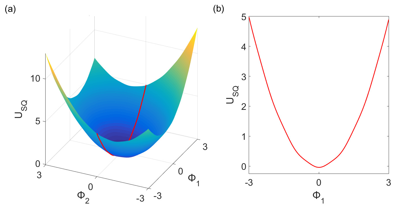
Figure 2: (a) The potential $U_{SQ}(\phi_{1},\phi_{2})$ of the SQUID dimer for $\tau=T=2\pi/\Omega$ where $\Omega=0.891$. (b) The corresponding one-dimensional projection of $U_{SQ}(\phi_{1},\phi_{2})$ on the $\phi_{2}=0$ plane. Other parameters: $\lambda=0.31$, $\phi_{ac}=0.02$, $\gamma=0.024$, and $\beta=0.1369$.

In the lossless case, i.e., when $\gamma=0$ ($R\rightarrow\infty$), the (Newtonian) dynamics of the SQUID dimer is governed by the equations

$$\ddot{\phi}_{1}=-\frac{\partial U_{SQ}(\phi_{1},\phi_{2})}{\partial\phi_{1}},\qquad\ddot{\phi}_{2}=-\frac{\partial U_{SQ}(\phi_{1},\phi_{2})}{\partial\phi_{2}}$$ (12)

in terms of the SQUID dimer potential

$$U_{SQ}(\phi_{1},\phi_{2}) = -\frac{1}{1+\lambda}\left(\phi_{1}+\phi_{2}\right)\phi_{ext}(\tau)$$ (13)

$$-\frac{\beta}{2\pi}\left[\cos(2\pi\phi_{1})+\cos(2\pi\phi_{2})\right]$$

$$+\frac{1}{2(1-\lambda^{2})}\left(\phi_{1}^{2}-2\lambda\phi_{1}\phi_{2}+\phi_{2}^{2}\right).$$

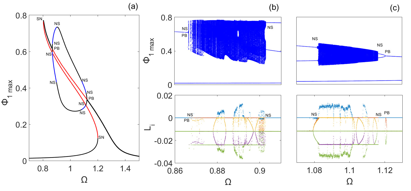
Figure 3: (a) The resonance curve of the SQUID dimer. Black lines correspond to stable branches and red and blue lines correspond to unstable ones. The latter are born through saddle-node bifurcations of limit cycles (SN), Neimark-Sacker bifurcations (NS), or pitchfork bifurcations of limit cycles (PB). (b) Maximum values of the magnetic flux $\phi_{1}$ (top) and all five Lyapunov exponents (bottom), as a function of the driving frequency in the interval corresponding to the left blue branches of (a). For each value of $\Omega$, $n_{i}=50$ different initial conditions were used. (c) The same as in (b) for the right blue branches of (a). Other parameters: $\lambda=0.31$, $\phi_{ac}=0.02$, $\gamma=0.024$, and $\beta=0.1369$.

Since the SQUID dimer considered here consists of two identical non-hysteretic SQUIDs ($2\pi\beta<1$), the potential $U_{SQ}(\phi_{1},\phi_{2})$ is a two-dimensional corrugated parabola with a single minimum that depends periodically on time $\tau$. A snapshot of the potential at $\tau=T$, with $T=2\pi/\Omega$ being the period of the (driving) external periodic field, is shown in Fig. 2(a) while its one-dimensional projection on the $\phi_{2}=0$ plane is shown in Fig. 2(b).

In what follows, the external dc flux is set to zero, i.e., $\phi_{dc}=0$. For obtaining the values of the SQUID-dependent normalized parameters $\beta$ and $\gamma$ that go into the model equations (II) and (II), we choose $L=120~{}pH$, $C=1.1~{}pF$, $R=500~{}\Omega$, and $I_{c}=2.35~{}\mu A$ for their equivalent lumped-circuit elements. These values are typical for non-hysteretic SQUIDs investigated recently in the context of SQUID metamaterials Trepanier2013 ; Zhang2015 . By substituting them into Eq. (11), we get $\beta_{L}=0.86$ ($\beta\simeq 0.1369$) and $\gamma=0.024$, while the $LC$ or geometrical frequency is $f_{LC}=\omega_{LC}/(2\pi)\simeq 13.9~{}GHz$. As mentioned earlier, the value of the coupling strength $\lambda$ depends significantly on the relative positions of the two SQUIDs, and may assume its value from the relatively broad range of $[-0.06,+0.50]$ that corresponds to technologically feasible SQUID dimer designs Anlage0000 . Besides, there are also the parameters $\phi_{ac}$ and $\Omega$ ($\phi_{dc}=0$), which can be tuned externally. Here, however, we prefer to fix the former to $\phi_{ac}=0.02$, which is well into the range of the experimentally accessible values, and use $\lambda$ and $\Omega$ as control parameters.

III Bifurcations, Quasi-periodicity, and Chaos

It is known that for relatively high $\phi_{ac}$, the single SQUID exhibits a multistable response which is reflected in its corresponding “snake-like” resonance curve Hizanidis2018 , i.e., the curve formed by the maximum flux within one driving period $T=2\pi/\Omega$, $\phi_{max}$, as a function of the driving frequency $\Omega$. For the value of $\phi_{ac}=0.02$ considered here, the single SQUID is bistable. When two SQUIDs are coupled positively (i.e., when $\lambda>0$) the bistability is maintained but the dynamics presents additional complexity. The resonance curve for the SQUID dimer is plotted in Fig. 3(a) in terms of the magnetic flux $\phi_{1}$ threading the loop of the SQUID number $1$. Specifically, the maximum flux threading the loop of the SQUID number $1$ within one driving period $T$, $\phi_{1,max}$, is plotted against the driving frequency $\Omega$. We see the typical tilted curve associated with bistability and hysteresis, where two stable solutions (black curves) coexist with an unstable one (red curve) below the geometric resonance frequency $\Omega=1$. Starting at lower driving frequencies and following the periodic solution in $\Omega$ there is a saddle-node bifurcation of limit cycles (SN) occurring at $\Omega=1.2$. The solution then becomes unstable and when it reaches the peak of the resonance curve it turns stable again in a second SN bifurcation at $\Omega=0.8036$. The stable branch that is born then undergoes a pitchfork bifurcation of limit cycles (PB) at $\Omega=0.8684$, where in addition to the unstable branch two more stable branches of periodic solutions are born. These branches consecutively become unstable in a Neimark-Sacker bifurcation (NS) on either side at $\Omega=0.87$, shown in blue color. The blue branches become stable again in a second NS bifurcation at $\Omega=0.8944$, again on either side. The same scenario takes place at $\Omega=1.12$ (right PB) and this family of solutions emanating from the two “opposite to each other” PB bifurcations, undergoes NS bifurcations (at $\Omega=1.083$ and $\Omega=1.114$) on either side forming, thus, a closed loop. The bifurcation lines have been obtained using a very powerful software tool that executes a root-finding algorithm for continuation of periodic solutions ENG02 .

We focus now on the two $\Omega$ intervals corresponding to the blue unstable branches of Fig. 3(a) which lie within the two PB bifurcations on both right and left side. In the upper panels of Figs. 3(b) and (c) the maxima of the solution for $\phi_{1}(\tau)$ are plotted over $\Omega$ for the left and right interval, respectively. Note that at each frequency $\Omega$, a large number of different initial conditions $n_{i}$ were used (here $n_{i}=50$) in order to obtain all the coexisting solutions within the $\Omega$ interval shown, and also to obtain a good representation of possible chaotic behavior. Apparently, chaotic behavior appears in both the upper panels of Figs. 3(b) and (c). These solution branches coexist with the blue unstable branches of Fig. 3(a) mentioned above; the reason for which they are not superposed to them is merely clarity.

In the corresponding lower panels, the Lyapunov exponents of the obtained solutions that are plotted for the same intervals of $\Omega$, reveal chaotic behavior in the regions where the maximum Lyapunov exponent $L_{1}$ is positive (positive Lyapunov exponents are shown as blue points). Careful inspection of the Lyapunov exponents indicate that transitions to chaos through quasiperiodicity and reversely take place in Figs. 3(b) and (c) (see next section). The Lyapunov exponents were calculated employing the algorithm from Geist1990 using the Julia^R software library. Similar multibranched resonance curve are sometimes encountered in dissipative-driven oscillators Warminski2015 ; Marchionne2018 ; Zang2019 where in addition, isolated branches (“isolas”) may exist. However, to the best of our knowledge, multibranched resonance curves whose branches are connected through Neimark-Sacker bifurcations have never before been observed.

Since the system dynamics is very sensitive to initial conditions, we have identified the basins of attraction of chaotic and periodic behavior for two $\Omega$ values within the intervals shown in Figs. 3(b) and (c) close to the NS bifurcations of limit cycles. These are displayed in Figs. 4(a) and (b), respectively, both in the $(\phi_{1},\phi_{2})$ plane (left panels) and $(\dot{\phi}_{1},\dot{\phi}_{2})$ plane (right panels). Blue (dark) regions denote the set of initial conditions leading to chaotic motion, while light yellow (light) regions the ones leading to periodic or quasiperiodic oscillations. The other state variables are initially fixed as $\dot{\phi}_{1}(\tau=0)=\dot{\phi}_{1}(\tau=0)=0$ and ${\phi}_{1}(\tau=0)={\phi}_{1}(\tau=0)=0$, respectively. In Fig. 4(a), an interesting intertwining between the basins of attraction of chaotic and periodic or quasiperiodic states can be seen. This is apparent from the presence of yellow spots located erratically within the blue regions in both subfigures, that resemble riddled basins investigated in various low-dimensional systems Lai1994 ; Sathiyadevi2019 . The inset of Fig. 4(a) reveals this intricate structure of the basin of attraction on a smaller scale. Note that a classification of basins of attraction in several low-dimensional systems has been perormed in Ref. Sprott2015 . The knowledge of the basins is essential for determining the usefulness of the systems in practical applications.

The other control parameter in our system is the coupling strength $\lambda$, which (as described in Section II) can obtain both negative and positive values within a certain range provided by calculations on feasible SQUID dimer designs Anlage0000 . In Fig. 6(a) the co-dimension 2 bifurcation diagram is shown in the $(\Omega,\lambda)$ parameter plane. Black lines mark the continuation of the saddle-node bifurcations and red lines that of the Neimark-Sacker (torus) bifurcations. In Fig. 6(b) the maximum Lyapunov exponent is plotted in the $(\Omega,\lambda)$ parameter space. Blue and yellow regions correspond to chaotic (positive $L_{\text{max}}$) and non-chaotic (negative or zero $L_{\text{max}}$) dynamics, respectively. We can see that the chaotic regimes lie within the boundaries of the NS bifurcation curves. In the following section we explore in detail the transition from quasiperiodicity to chaos in our system.

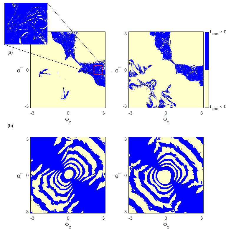
Figure 4: Basins of attraction for the SQUID dimer in terms of the maximum Lyapunov exponent $L_{\text{max}}$. Blue and yellow color corresponds to chaotic and non-chaotic dynamics, respectively. Left: $\phi_{1}$ versus $\phi_{2}$ for $(\dot{\phi}_{1}(0),\dot{\phi_{2}}(0))=(0,0)$. Right: $\dot{\phi}_{1}$ versus $\dot{\phi}_{2}$ for $(\phi_{1}(0),\phi_{2}(0))=(0,0)$. (a) $\Omega=0.891$, and (b) $\Omega=1.1$. The inset in the left panel of (a) shows a blow-up of the region inside the red box. Other parameters: $\lambda=0.31$, $\phi_{ac}=0.02$, $\gamma=0.024$, and $\beta=0.1369$.

IV Torus-doubling transition to chaos

From Figs. 3(b)-(c) and  5(b) it is clear that the SQUID dimer described by Eqs. (II) and (II) becomes chaotic through Neimark-Sacker bifurcations. This quasiperiodic transition to chaos is a well-known scenario whereby a torus in low-dimensional dynamical systems loses its stability and develops into chaos. A path from a limit cycle, then a transition into 2D torus following by a 3D torus and eventually direct transition to chaos has been presented numerically and experimentally is an analog electrical circuit representing the ring of unidirectionally coupled single-well Duffing oscillators Borkowski2015 . Another possible scenario to chaos is a cascade of period doublings of the torus which has been investigated numerically long ago using low-dimensional maps Arneodo1983 ; Kaneko1984 , and experimentally in electrochemical reactions Bassett1989 . According to the second scenario, a finite cascade of period doubling of such invariant tori leads eventually to chaos. This scenario has been reported numerically for a quintic complex Ginzburg-Landau equation Kim1997 and bimodal laser model Letellier2007 as well as experimentally, in Rayleigh-Benard convection Flesselles1994 , in a simple thermoacoustic system Mondal2017 , and near the ferroelectric phase transition of $KH_{2}PO_{4}$ crystals Shin1999 .

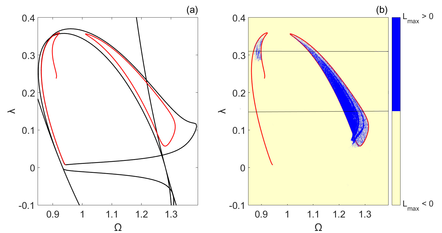
Figure 5: (a) Bifurcation diagram in the ($\Omega,\lambda$) parameter plane of the two coupled SQUIDs. Black and red lines correspond to saddle-node (SN) bifurcations of limit cycles and Neimark-Sacker (NS) bifurcations, respectively. (b) Map of the maximum Lyapunov exponent $L_{\text{max}}$ in the ($\Omega,\lambda$) parameter space, on which the NS bifurcation curve from (a) is superposed (red lines). Blue and yellow color corresponds to chaotic and non-chaotic dynamics, respectively. Other parameters: $\phi_{ac}=0.02$, $\gamma=0.024$, and $\beta=0.1369$.

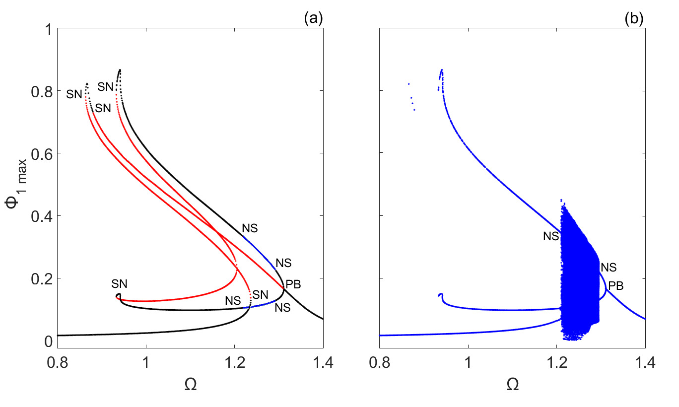
Figure 6: (a) The resonance curve of the SQUID dimer for $\lambda=0.15$. Black lines correspond to stable branches and red and blue lines correspond to unstable ones. The latter are born through saddle-node bifurcations of limit cycles (SN), Neimark-Sacker bifurcations (NS), or pitchfork bifurcations of limit cycles (PB). (b) Maximum values of the magnetic flux $\phi_{1}$ of stable solutions as a function of the driving frequency in the same $\Omega$ interval. Other parameters: $\phi_{ac}=0.02$, $\gamma=0.024$, and $\beta=0.1369$.

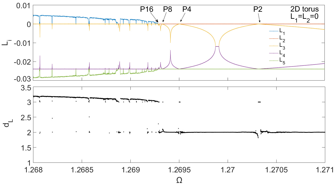
Figure 7: The complete set of Lyapunov exponents $L_{i}$, $i=1,...,5$ for the SQUID dimer (top) and the corresponding Lyapunov dimension (bottom), as a function of the driving frequency $\Omega$. The bifurcation analysis depicts a transition from a stable two-dimensional torus to chaos via a sequence of four consecutive period-doubling bifurcations marked by $P_{i}$ ($i=2,4,8,16$), where the period of the solution doubles. Other parameters: $\lambda=0.15$, $\phi_{ac}=0.02$, $\gamma=0.024$ and $\beta=0.1369$.

We examine this route to chaos through period doubling of a 2D torus in our system by fixing the magnetic coupling strength to a certain value $\lambda=0.15$ (marked by a black horizontal line in Fig. 5(b)) and by varying the driving frequency $\Omega$ in a narrow interval that encloses chaotic states.

For this choice of parameters, the resonance curve (Fig. 6(a)) exhibits the same sequence of bifurcations (PB and consequently NS) as in Fig. 3(a), but presents no second chaotic band and therefore no “bubble” connected to it. The transition into chaos is shown in Fig. 6(b) where the maximum values of the magnetic flux $\phi_{1}$ are plotted for the same $\Omega$ interval.

For each value of $\Omega$ the whole spectrum of the Lyapunov exponents is calculated and plotted in Fig. 7 (top). Starting from the right end of the frequency interval, it is observed that the two largest Lyapunov exponents are zero ($L_{1}=L_{2}=0$), while the other three are less than zero. This indicates quasiperiodic dynamics on a stable 2D torus. When the frequency $\Omega$ decreases, one more Lyapunov exponent reaches zero at $\Omega=1.27032$ (marked as P2 on the figure), indicating a period doubling bifurcation of the torus. By further decreasing $\Omega$, we find three more points in which the three largest Lyapunov exponents are zero at $\Omega=1.269505$, $1.26933$, and $1.269295$ indicating three more period doupling bifurcations of the 2D torus (marked by P4, P8, and P16, respectively, on the figure). For frequencies even lower than that at P16 the 2D torus break down and the system enters into a chaotic state, as it is indicated by the positivity of the largest Lyapunov exponent ($L_{1}=L_{max}>0$). This transition to chaos is also reflected in the Lyapunov dimension $d_{L}$, which according to Kaplan and York KAP79 is given by:

$$d_{L}=k+\frac{1}{|L_{k+1}|}\sum_{i=1}^{k}L_{i},$$ (14)

where $k$ is defined by the condition that

$$\sum_{i=1}^{k}L_{i}\geq 0~{}~{}~{}{\rm and}~{}~{}~{}\sum_{i=1}^{k+1}L_{i}<0.$$ (15)

As the 2D torus transitions into chaos, the Lyapunov dimension changes from the value $d_{L}=2$ to $d_{L}>3$, as shown in Fig. 7 (bottom).

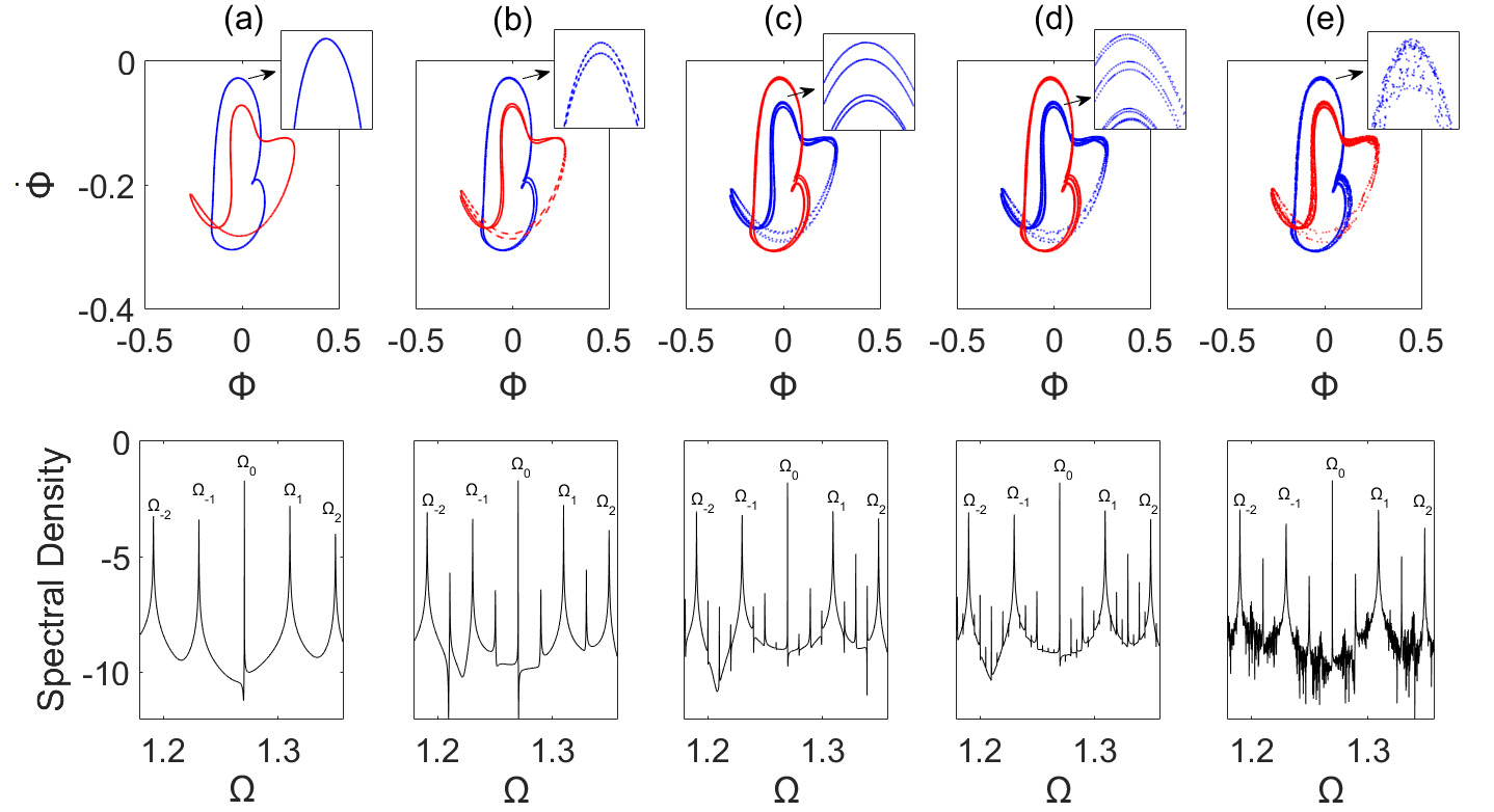
Figure 8: Poincaré cross sections on the $\Phi-\dot{\Phi}$ plane (upper panels) and the corresponding frequency spectra plotted in a logarithmic scale (bottom panels), for (a) $\Omega=1.2705$; (b) $\Omega=1.27$; (c) $\Omega=1.2694$;(d) $\Omega=1.26931$; (e) $\Omega=1.26923$. In the upper panels, blue and red lines correspond to the first ($\Phi=\phi_{1}$, $\dot{\Phi}=\dot{\phi}_{1}$) and second ($\Phi=\phi_{2}$, $\dot{\Phi}=\dot{\phi}_{2}$) SQUID, respectively. Insets: Enlargement of a small part of Poincaré sections of the trajectories of the first SQUID to make clear the period of the tori. Other parameters as in Fig. 7.

Typical Poincaré sections of the period-2, -4, -8, and chaotic 2D tori on the $\phi_{1,2}-\dot{\phi}_{1,2}$ phase plane are shown in the upper panels of Figs. 8(a) - (e). Blue and red lines correspond to flux threading the loop of the first ($1$) and the second ($2$) SQUID, respectively. The insets show enlargements of a small part of the Poincaré sections of the first SQUID (SQUID number $1$), in order to see clearly the varying number of layers of the tori as the frequency $\Omega$ decreases. The Poincaré section of the period-16 torus is very similar to that of the period-8 torus and thus it has been omitted. In the lower panels of Fig. 8, the corresponding Fourier power spectral densities in a logarithmic scale are shown. The 2D torus (upper panel of Fig. 8(a)) has a dominant frequency which in the present case coincides with the external (driving) frequency $\Omega$, as well as four more frequencies denoted as $\Omega_{\pm 1}$, $\Omega_{\pm 2}$ (lower panel of Fig. 8(a)). The exact values of these frequencies are obtained from the locations of the sharp peaks. Then, as the period of the 2D torus increases to $2$, $4$, and $8$ through period-doubling bifurcations, a doubling of the sharp peaks occurs (as can be seen in Fig. 8(b), (c), and (d), respectively) that correspond to frequencies with significant spectral content. In Fig. 8(e), in which the SQUID dimer is in a chaotic state, the power spectrum exhibits a substantial noisy background, along with several sharp peaks that correspond to frequencies with significant spectral content. Note that the driving frequency $\Omega$ is dominant in all five subfigures.

Thus, we have identified a novel route to chaos for the SQUID dimer, which initiates from a single limit cycle. The latter then bifurcates into a 2D torus, which follows a finite period doubling cascade which eventually leads to a chaotic state. Note that in the case of two coupled Duffing oscillators with dissipation and driving force, three period-doubling bifurcations of a three-torus were identified for the transition to chaos through quasiperiodicity Kozlowski1995 .

V Localized $\&$ Chaotic Synchronization

The SQUID dimer considered here consists of two symmetrically coupled identical nonlinear oscillators. Such systems were once believed to support only totally synchronous or asynchronous states. However, as it is known today, there are more possible forms of synchronization such as the so called localized synchronization. This form of synchronization has been originally investigated in a slightly dissimilar pair of solid state Kuske1997 and semiconductor Hohl1997 lasers. For two coupled oscillators, localized synchronization means that one of the oscillators exhibits strong oscillations while the other one exhibits weak oscillations. In the other limit, that of asynchronous dynamics, extreme case of having the one oscillator exhibiting periodic motion and the other chaotic motion has been recently reported Awal2019 . We explore below the effect of localized synchronization for the SQUID dimer using the correlation function between the time-dependent fluxes through the loop of the first and the second SQUID $\phi_{1}(t)$ and $\phi_{2}(t)$, respectively, i.e.,

$$C_{12}=\frac{\langle(\phi_{1}(t)-\mu_{1})(\phi_{2}(t)-\mu_{2})\rangle}{\sigma_{1}\sigma_{2}},$$ (16)

where $\mu_{1,2}$ and $\sigma_{1,2}$ are the mean value and the standard deviation of the corresponding time series of $\phi_{1}$ and $\phi_{2}$, respectively. Using this measure we can quantify the asymmetry in the amplitudes of the two coupled SQUID magnetic fluxes. If $\phi_{1}$ and $\phi_{2}$ are increasing or decreasing simultaneously then the correlation function will be positive. In contrast, if the value of $\phi_{1}$ is increasing while $\phi_{2}$ is decreasing and vice versa, then $C_{12}$ is negative. The maximum/minimum value of the correlation function is $\pm 1$. For $C_{12}\simeq 1$ the time series of $\phi_{1}$ and $\phi_{2}$ are almost identical thereby the two SQUIDs exhibit in-phase synchronization, whereas for $C_{12}\simeq-1$ they are in anti-phase synchronization.

In Fig. 9(a), the asymptotic value of the correlation function $C_{12}$ is mapped onto the $\Omega,\lambda$ parameter space. As mentioned earlier, the value of $C_{12}$ reflects the dynamical behavior of the SQUID dimer as long as its synchronization properties are concerned. As it can be observed, the value of $C_{12}$ is equal to $1$ in a large area (yellow) of the parameter space but there also exist regions where $C_{12}\neq 1$. For example, a dark-blue region (1) can be observed in which $C_{12}$ approaches $-1$, indicating anti-synchronized (i.e., phase difference $\pi$ between $\phi_{1}(t)$ and $\phi_{2}(t)$) dynamics. Moreover, we observe a “horn”-shaped region of intermediate to high values of $C_{12}$ which coincides with the corresponding “horn”-shaped chaotic region of Fig. 6(b). This particular region, which is bounded by the Neimark-Sacker (NS) bifurcation lines, intermittent chaotic synchronization Baker1998 ; Zhao2005 is observed. In the case of the SQUID dimer, the effect of intermittent chaotic synchronization is manifested by the entrainment of the two SQUID time series for $\phi_{1}(t)$ and $\phi_{2}(t)$ in random temporal intervals of finite duration Zhao2005 . This will be further investigated in future works involving SQUID trimers where more interesting synchronization phenomena can be observed, like small chimeras Banerjee2018 .

Next we focus on the behavior of the correlation function $C_{12}$ in the non-chaotic region of the $(\Omega,\lambda)$ parameter space and reveal another interesting behavior. For a fixed $\Omega$ we study the dependence of $C_{12}$ as the coupling strength $\lambda$ varies from region 1 to 2 of Fig. 9(a). A cross section of $C_{12}$ for $\Omega=0.9822$ is plotted in Fig. 9(b) in red color, for one random set of initial conditions (top) and $n_{i}=30$ sets of different, randomly chosen initial conditions (bottom). The difference between the maximum values of the two SQUID magnetic fluxes $\phi_{1\text{max}}-\phi_{2\text{max}}$ is also plotted in black color. We make the following observations: first of all, the fully phase-synchronized state ($C_{12}=1$) exists for all $\lambda$ in this interval. Secondly, the correlation function appears to have a (co)sinusoidal dependence on the coupling strength $\lambda$ as expected, since the correlation function of two out-of-phase cosine signals is a cosine function of their phase difference Oppenheim1996 . In the low-coupling non-chaotic regions 1 and 2 we can assume that the two SQUID solutions are also (co)sine-like. For $\phi_{1}(t)$ and $\phi_{2}(t+\tau)$ or vice versa for $\phi_{1}(t+\tau)$ and $\phi_{2}(t)$, $\tau$ is the phase difference between the SQUID fluxes and is dependent on the set of initial conditions. From Fig. 9(b) (bottom) we may claim that the $\tau=0$ case corresponds to $C_{12}=1$ and the (co)sinusoidal-like form of $C_{12}$ corresponds to the case where $\tau$ is a function of $\lambda)$. In the former case the two SQUIDs are in phase and $\phi_{1\text{max}}-\phi_{2\text{max}}$ is zero, while in the latter case their phase difference varies from values close to $-1$ (almost anti-phase) to values close to $+1$ (almost in-phase). The difference $\phi_{1\text{max}}-\phi_{2\text{max}}$ attains a nonzero positive/negative value depending on whether $\phi_{1}$ is larger/smaller than $\phi_{2}$, for all $\lambda$ and all initial conditions. Therefore this case corresponds to an asymmetric solution as far as the amplitudes of the two coupled SQUIDs are concerned.

This is illustrated in Fig. 9(c) in the phase portraits (top) and time series (bottom) of the magnetic flux for the first SQUID (green line) and the second SQUID (blue line) for parameters tha belong to region 1 $(\lambda=-0.0398,C_{12}=-0.9103)$ and region 2 $(\lambda=0.0672,C_{12}=0.9248)$. These plots show the phase portraits of the corresponding stable periodic solutions where large asymmetry in the amplitudes of the two coupled SQUIDs occurs. Due to that difference between the amplitudes, these two states are illustrative examples of localized synchronization. Moreover, through the time series, it can be clearly seen that the fluxes $(\phi_{1}$ and $\phi_{2})$ are almost out of phase (I) and almost in phase (II) because the correlation function has values close to $-1$ and $1$, respectively.

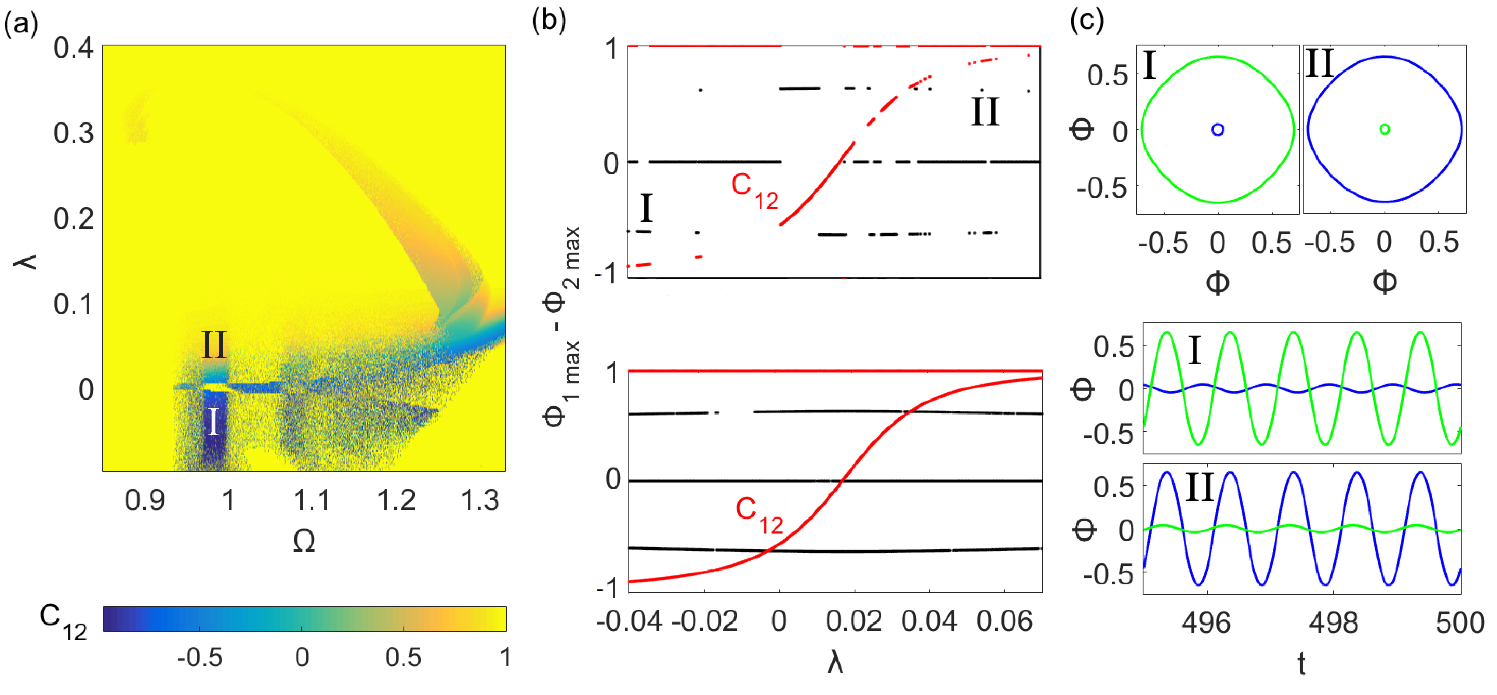
Figure 9: (a) Dynamical behavior in the ($\Omega,\lambda$) parametric space of the correlation function $C_{12}$. For a completely in-phase synchronized state $C_{12}=1$ while for a completely anti-phase synchronized state $C_{12}=−1$. (b) The correlation function (red line) and maxima differences between $\phi_{1}$ and $\phi_{2}$ (black line), versus the coupling strength ($\lambda$), for one random set of initial conditions (top) and for $n_{i}=30$ different initial conditions (bottom) where $\Omega=0.9822$. (c) Phase portraits (top) and time series (bottom) of the magnetic flux for the first SQUID, $\phi_{1}$ (green line), and the second SQUID, $\phi_{2}$ (blue line), for (I) $\lambda=-0.0398$, $C_{12}=-0.9103$; (II) $\lambda=0.0672$, $C_{12}=0.9248$. Other parameters $\phi_{ac}=0.02$, $\gamma=0.024$, and $\beta=0.1369$.

VI Conclusions

In summary, a dimer comprising two magnetically coupled SQUIDs is investigated numerically with respect to its bifurcation structure and its transitions from quasiperiodicity to chaos through a finite period-doubling cascade of tori. The SQUID dimer is a prototype, dissipative-driven dynamical system of considerably complex dynamic behavior, on which numerous nonlinear dynamic effects can be investigated. In the present work, the bifurcation structure of the SQUID dimer was obtained using the driving frequency $\Omega$ and the coupling strength $\lambda$ as external control parameters that form a two-dimensional parameter space. Bifurcation (stroboscopic) diagrams as a function of $\Omega$ reveal multibranched resonance curves resulting through different kinds of bifurcations, transitions to chaos after four period-doubling bifurcations of a 2D torus, and riddle-like basins. Bifurcation diagrams for SN and NS bifurcations are shown on the $\Omega-\lambda$ plane. In combination with maps of the maximum Lyapunov exponent $\Lambda_{max}$, it is observed that the areas of the $\Omega-\lambda$ plane where chaotic behavior is expected is bounded by the NS bifurcation curves. Eventually, localized synchronization is observed and quantified in the SQUID dimer using the correlation function $C_{12}$. The possibility of intermittent chaotic synchronization is briefly mentioned.

- (1) Jan Awrejcewicz, “Bifurcation And Chaos In Coupled Oscillators,” World Scientific, Singapore (1991).
- (2) M. Rosenblum and A. Pikovsky, “Synchronization: from pendulum clocks to chaotic lasers and chemical oscillators,” Contemporary Physics 44 (5), 401-416 (2003).
- (3) K. Wiesenfeld and P. Hadley, “Attractor crowding in oscillator arrays,” Phys. Rev. Lett. 62, 1335-1338 (1989).
- (4) Y. Nishio and S. Mori, “Mutually coupled oscillators with an extremely large number of steady states,” IEEE Xplore, 819-822 (1992).
- (5) R. Jothimurugan, K. Thamilmaran, S. Rajasekar, and M. A. F. Sanjuán, “Multiple resonance and anti-resonance in coupled Duffing oscillators,” Nonlinear Dyn. 83 1803-1814 (2016).
- (6) Y. Kominis, K. D. Choquette, A. Bountis, and V. Kovanis, “Antiresonances and Ultrafast Resonances in a Twin Photonic Oscillator,” IEEE Photonics Journal 11 (1), 1500209 (2019).
- (7) Prasun Sarkar and Deb Shankar Ray, “Vibrational antiresonance in nonlinear coupled systems,” Phys. Rev. E 99, 052221 (2019).
- (8) Hua-Wei Yin, Jian-Hua Dai, and Hong-Jun Zhang, “Phase effect of two coupled periodically driven Duffing oscillators,” Phys. Rev. E 58 (5), 5683-5688 (1998).
- (9) A. Kenfack, “Bifurcation structure of two coupled periodically driven double-well Duffing oscillators,” Chaos Soliton Fract. 15, 205-218 (2003).
- (10) N. Lazarides, M. I. Molina, G. P. Tsironis, and Yu. S. Kivshar, “Multistability and localization in coupled nonlinear split-ring resonators,” Phys. Lett. A 374, 2095-2097 (2010).
- (11) Y. Kominis, K. D. Choquette, A. Bountis, and V. Kovanis, “Exceptional points in two dissimilar coupled diode lasers,” Appl. Phys. Lett. 113, 081103 (2018).
- (12) E. Tafo Wembe and R. Yamapi, “Chaos synchronization of resistively coupled Duffing systems: Numerical and experimental investigations,” Commun. Nonlinear Sci. Numer. Simul. 14, 1439-1453 (2009).
- (13) R. Herrero, M. Figueras, J. Rius, F. Pi, and G. Orriols, “Experimental observation of the amplitude death effect in two coupled nonlinear oscillators,” Phys. Rev. Lett. 84 (23), 5312-5315 (2000).
- (14) A. Hohl, A. Gavrielides, T. Erneux, and V. Kovanis, “Localized synchronization in two coupled nonidentical semiconductor lasers,” Phys. Rev. Lett. 78 (25), 4745-4748 (1997).
- (15) T. Kapitaniak and W.-H. Steeb, “Transition to hyperchaos in coupled generalized van der Pol equations,” Phys. Lett. A 152 (1,2), 33-36 (1991).
- (16) T. Kapitaniak, K.-E. Thylwe, I. Cohen, and J. Wojewoda, “Chaos-Hyperchaos Transition,” Chaos Soliton Fract. 5 (10), 2003-2011 (1995).
- (17) T. Kapitaniak, Y. Maistrenko, and S. Popovych, “Chaos-hyperchaos transition,” Phys. Rev. E 62 (2), 1972-1976 (2000).
- (18) K. Grygiel and P. Szlachetka, “Chaos and hyperchaos in coupled Kerr oscillators,” Optics Communications 177, 425-431 (2000).
- (19) Prof. S. M. Anlage (Personal communication) and also https://snf.ieeecsc.org/sites/ieeecsc.org/files/documents/snf/abstracts/Anlage_STP647.pdf, p. 33.
- (20) D. Rand, S. Ostlund, J. Sethna, and E. D. Siggia, “Universal transition from quasiperiodicity to chaos in dissipative systems,” Phys. Rev. Lett. 49 (2), 132-135 (1982).
- (21) A. R. Bishop, M. G. Forest, D. W. McLaughlin, E. A. Overman II, “A quasi-periodic route to chaos in a near-integrable PDE,” Physica 23D, 293-328 (1986).
- (22) T. W. Dixon, T. Gherghetta, and B. G. Kenny, “Universality in the quasiperiodic route to chaos,” Chaos 6 (1), 32-42 (1996).
- (23) Z. Elhadj and J. C. Sprott, “A minimal 2-D quadratic map with quasiperiodic route to chaos,” Int. J. Bifurc. Chaos 18 (5), 1567-1577 (2008).
- (24) L. Borkowski, P. Perlikowski, T. Kapitaniak, and A. Stefanski, “Experimental observation of three-frequency quasiperiodic solution in a ring of unidirectionally coupled oscillators,” Phys. Rev. E 91, 062906 (2015).
- (25) J. Kozlowski, U. Parlitz, and W. Lauterborn, “Bifurcation analysis of two coupled periodically driven Duffing oscillators,” Phys. Rev. E 51(3), 1861-1867 (1995).
- (26) R. Kleiner and D. Koelle and F. Ludwig and J. Clarke, “Superconducting quantum interference devices: State of the art and applications,” Proceedings of the IEEE 92, 1534-1548 (2004).
- (27) R. L. Fagaly, “Superconducting quantum interference device instruments and applications,” Rev. Sci. Instrum. 77, 101101 (2006).
- (28) J. Hizanidis, N. Lazarides, and G.P. Tsironis, “Flux bias-controlled chaos and extreme multistability in SQUID oscillators,” Chaos 28, 063117 (2018).
- (29) M. Trepanier, D. Zhang, O. Mukhanov, and S. M. Anlage, “Realization and modeling of RF superconducting quantum interference device metamaterials,” Phys. Rev. X 3, 041029 (2013).
- (30) D. Zhang, M. Trepanier, O. Mukhanov, and S. M. Anlage, “Broadband transparency of macroscopic quantum superconducting metamaterials,” Phys Rev X 5, 041045 (2015).
- (31) N. Lazarides, G. Neofotistos, and G. P. Tsironis, “Chimeras in SQUID Metamaterials,”, Phys. Rev. B 91, 054303 (2015).
- (32) J. Hizanidis, N. Lazarides, and G. P. Tsironis, “Robust chimera states in SQUID metamaterials with local interactions”, Phys. Rev. E 94, 032219 (2016).
- (33) J. Hizanidis, N. Lazarides, G. Neofotistos, and G. P. Tsironis, “Chimera states and synchronization in magnetically driven SQUID metamaterials”, Eur. Phys. J. Special Topics, Springer 225, 1231 (2016).
- (34) J. Hizanidis, N. Lazarides, and G. P. Tsironis, “Pattern formation and chimera states in 2D SQUID metamaterials ”, Chaos 30, 013115 (2020).
- (35) M. Agaoglou, V. M. Rothos, and H. Susanto, “Homoclinic chaos in a pair of parametrically-driven coupled SQUIDs,” J. Phys. Conf. Ser. 574, 012027 (2015).
- (36) M. Agaoglou, V. M. Rothos, and H. Susanto, “Homoclinic chaos in coupled SQUIDs,” Chaos Soliton Fract. 99, 133-140 (2017).
- (37) M. Bier and T. C. Bountis, “Remerging Feigenbaum Trees in Dynamical Systems,” Phys. Lett. 104, 239 (1984).
- (38) B. D. Josephson, “Possible new effects in superconductive tunnelling,” Phys. Lett. A 1, 251-253 (1962).
- (39) K. K. Likharev, “Dynamics of Josephson Junctions and Circuits,” Gordon and Breach, Philadelphia (1986).
- (40) K. Engelborghs, T. Luzyanina, and D. Roose, “Numerical bifurcation analysis of delay differential equations using DDE-BIFTOOL,” ACM Trans. Math. Softw. 28, 1 (2002).
- (41) K. Geist, U. Parlitz, and W. Lauterborn, “Comparison of different methods for computing Lyapunov exponents,” Prog. Theor. Phys. 83 (5), 875-893 (1990).
- (42) J. Warminski, “Frequency locking in a nonlinear MEMS oscillator driven by harmonic force and time delay,” Int. J. Dynam. Control 3, 122-136 (2015).
- (43) A. Marchionne, P. Ditlevsen, and S. Wieczorek, “Synchronisation vs. resonance: Isolated resonances in damped nonlinear oscillators,” Physica D 380-381, 8-16 (2018).
- (44) Jian Zang and Ye-Wei Zhang, “Responses and bifurcations of a structure with a lever-type nonlinear energy sink,” Nonlinear Dyn. 98, 889-906 (2019).
- (45) Ying-Cheng Lai and R. L. Winslow, “Riddled Parameter Space in Spatiotemporal Chaotic DynamicalSystem,” Phys. Rev. Lett. 72 (11), 1640-1643 (1994).
- (46) K. Sathiyadevi, S. Karthiga, V. K. Chandrasekar, D. V. Senthilkumar, and M. Lakshmanan, “Frustration induced transient chaos, fractal and riddled basins in coupled limit cycle oscillators,” Commun. Nonlinear Sci. Numer. Simulat. 72, 586-599 (2019).
- (47) J. C. Sprott and Anda Xiong, “Classifying and quantifying basins of attraction,” Chaos 25, 083101 (2015).
- (48) A. Arneodo, P. H. Coullet, and E. A. Spiegel, “Cascade of period doubling tori,” Phys. Lett. A 94 (1), 1-6 (1983).
- (49) K. Kaneko, “Oscillation and doubling of torus,” Prog. Theor. Phys. 72 (2), 202-215 (1984).
- (50) M. R. Bassett and J. L. Hudson, “Experimental evidence of period doubling of tori during an electrochemical reaction,” Physica D 35, 289-298 (1989).
- (51) Jung-Im Kim, Hwa-Kyun Park, and Hie-Tae Moon, “Period doubling of a torus: Chaotic breathing of a localized wave,” Phys. Rev. E 55 (4), 3948-3951 (1997).
- (52) C. Letellier, M. Bennoud, and G. Martel, “Intermittency and period-doubling cascade on tori in a bimode laser model,” Chaos Soliton Fract. 33, 782-794 (2007).
- (53) J.-M. Flesselles, V. Croquette, and S. Jucquois, “Period doubling of a torus in a chain of oscillators,” Phys. Rev. Lett. 72 (18), 2871-2874 (1994).
- (54) S. Mondal, S. A. Pawar, and R. I. Sujith, “Synchronous behaviour of two interacting oscillatory systems undergoing quasiperiodic route to chaos,” Chaos 27, 103119 (2017).
- (55) Jong Cheol Shin, “Experimental observation of a torus-doubling transition to chaos near the ferroelectric phase transition of a crystal,” Phys. Rev. E 60 (5), 5394-5401 (1999).
- (56) H. Kaplan and J. A. Yorke, “Lecture Note in Mathematics,” Springer-Verlag, Berlin 730, 228-237 (1979).
- (57) R. Kuske and T. Erneux, “Localized synchronization of two coupled solid state lasers,” Optics Communications 139, 125-131 (1997).
- (58) N. M. Awal, D. Bullara, and I. R. Epstein, “The smallest chimera: Periodicity and chaos in a pair of coupled chemical oscillators,” Chaos 29, 013131 (2019).
- (59) G. L. Baker, J. A. Blackburn, and H. J. T. Smith, “Intermittent Synchronization in a Pair of Coupled Chaotic Pendula,” Phys. Rev. Lett. 81 (3), 554-557 (1998).
- (60) Liang Zhao, Ying-Cheng Lai, and Chih-Wen Shih, “Transition to intermittent chaotic synchronization,” Phys. Rev. E 72 (3), 036212 (2005).
- (61) A. Banerjee and D. Sikder, “Transient chaos generates small chimeras,” Phys. Rev. E 98, 032220 (2018).
- (62) A. V. Oppenheim and A. S. Willsky, with S. H. Nawab, “Signals and Systems (2nd Edition),” Pearson (1996).