Conformal invariance of weakly compressible two-dimensional turbulence

Abstract

We study conformal invariance of vorticity clusters in weakly compressible two-dimensional turbulence at low Mach numbers. On the basis of very high resolution direct numerical simulation we demonstrate the scaling invariance of the inverse cascade with scaling close to Kolmogorov prediction. In this range of scales, the statistics of zero-vorticity isolines are found to be compatible with those of critical percolation, thus generalizing the results obtained in incompressible Navier-Stokes turbulence.

I Introduction

The inverse energy cascade is a key feature of two-dimensional incompressible turbulence predicted by Kraichnan many years ago Kraichnan (1967). As a consequence of the existence of two inviscid quadratic invariants of the 2D incompressible Navier-Stokes equations, the enstrophy is transferred to small scales producing the direct cascade, while energy moves to large scales generating the inverse cascade. The inverse cascade in 2D incompressible turbulence has been observed in numerical simulations Herring and McWilliams (1985); Maltrud and Vallis (1991); Smith and Yakhot (1993); Boffetta et al. (2000); Xiao et al. (2009) and laboratory experiments Paret and Tabeling (1997); Rivera et al. (1998); Chen et al. (2006), and its scaling properties have been established including the almost Gaussian statistics of velocity fluctuations and the absence of intermittency Boffetta et al. (2000).

More recently, scaling invariance of the inverse cascade has been promoted to conformal invariance for some specific features of the turbulent field. In particular, by using the technique of stochastic-Löwner evolution (SLE), it has been shown that clusters of vorticity are statistically equivalent to those of critical percolation, one of the simplest universality classes in critical phenomena Bernard et al. (2006). This result, which suggests an intriguing connection between (non-equilibrium) turbulent flows and statistical models at the critical point, has been extended to other 2D incompressible flows, including surface quasi-geostrophic turbulence Bernard et al. (2007) and a class of active scalar turbulence Falkovich and Musacchio (2010). Conformal invariance has also been investigated experimentally in Lagrangian reconstructed vorticity field of a turbulent surface flow Stefanus et al. (2011) (two-dimensional section of a three-dimensional flow), where deviations from SLE predictions have been observed.

In this paper, we study the appearance of conformal invariance in the inverse cascade of weakly compressible 2D turbulence. Compressible two-dimensional turbulence has applications in numerous geophysical, astrophysical and industrial problems. Specifically, we consider a flow with an ideal-gas equation of state with the ratio of specific heats $\gamma=c_{v}/c_{p}\simeq 1$, which is relevant to astrophysical applications (where radiation provides for temperature equilibration) Falkovich and Kritsuk (2017) and for soap films when fluid velocities are of the order of the elastic wave speed in the limit of large Reynolds numbers Chomaz (2001).

This paper is organized as follows. In Section II, we introduce the physical model, its phenomenology and the numerical simulation. In Section III, we discuss the statistics of the inverse cascade, while Section IV is devoted to conformal analysis of isovorticity lines. Finally, Section V contains some conclusions.

II Model and phenomenology of 2D compressible flows

The dynamics of a compressible flow is given by the Euler equations, which impose the conservation of mass, momentum and total energy:

$$\partial_{t}\rho+\nabla\cdot\left(\rho{\bm{u}}\right)=0,$$ (1)

$$\partial_{t}\left(\rho{\bm{u}}\right)+\nabla\cdot\left(\rho{\bm{uu}}+p\bm{I}\right)={\bm{f}},$$ (2)

$$\partial_{t}\mathcal{E}+\nabla\cdot\left[\left(\mathcal{E}+p\right){\bm{u}}\right]={\bm{f}}\cdot{\bm{u}},$$ (3)

where $\rho$ is the density field, ${\bm{u}}$ the velocity, $p$ is the pressure, ${\bm{f}}$ is the external forcing, $\mathcal{E}=\rho\left(u^{2}/2+e\right)$ is the total energy density (the sum of kinetic and potential energy density), and $\bm{I}$ is the identity matrix. The system of equations (1-3) is closed by the equation of state for an idea gas $p=\left(\gamma-1\right)\rho e$. In the absence of external forcing ${\bm{f}}=0$, the system conserves the total energy $E=\int\mathcal{E}d{\bm{x}}$, which is given by the sum of the kinetic energy $K=(1/2)\int\rho u^{2}d{\bm{x}}$ and the potential energy $U=\int\rho ed{\bm{x}}$.

The average compressibility of the velocity field is quantified by the rms Mach number $M=\sqrt{\langle u^{2}\rangle}/c$, where $c$ is the speed of sound in the fluid. The velocity field can be decomposed into the solenoidal and irrotational components ${\bm{u}}={\bm{u}}_{s}+{\bm{u}}_{i}$, where ${\bm{\nabla}}\cdot{\bm{u}}_{s}=0$ and ${\bm{\nabla}}\times{\bm{u}}_{i}=0$.

In the case of a two-dimensional flow, they can be expressed in terms of two scalar fields: the stream function $\psi$, and the velocity potential $\phi$,

$${\bm{u}}_{s} = (\partial_{y}\psi,-\partial_{x}\psi),$$ (4)

$${\bm{u}}_{i} = {\bm{\nabla}}\phi\;.$$ (5)

The Laplacian of the velocity potential provides a local measure of the divergence of the velocity ${\bm{\nabla}}\cdot{\bm{u}}=\nabla^{2}\phi$, while the Laplacian of the stream functions defines the vorticity field $\omega=\partial_{x}u_{y}-\partial_{y}u_{x}=-\nabla^{2}\psi$.

The phenomenology of a 2D compressible flow is strongly dependent on the Mach number. In the low-compressibility regime ($M\ll 1$), the behavior is similar to that of the incompressible case. One observes the development of a double-cascade scenario in which the enstrophy $\Omega=(1/2)\int\omega^{2}\rho d{\bm{x}}$ is preferentially transferred toward small scales (direct cascade), while the kinetic energy is transferred mostly to large scales (inverse cascade). In the absence of a large-scale dissipation mechanism (such as friction), the inverse cascade process causes the accumulation of energy at the largest scale (smaller wavenumber) of the flow. The phenomenon of “spectral condensation” of kinetic energy on the lowest accessible wavenumber has been studied both in the 2D incompressible Smith and Yakhot (1993) and compressible flows Falkovich and Kritsuk (2017); Naugol’nykh (2014). It has also been observed in quasi-2D geometries, i.e. in the turbulent dynamics of thin layers Xia et al. (2009); Musacchio and Boffetta (2019).

The energy accumulation at large scales causes the growth in time of the Mach number, increasing the compressibility of the flow. A peculiar phenomenon of the compressible case is the formation of acoustic waves, i.e. pressure fluctuations which propagate within the fluid Lighthill (1955). Acoustic waves of sufficiently large amplitude break to form a train of N-waves. Emerging shocks in turn speed up the attenuation of acoustic energy. Shocks also amplify small-scale vorticity by compression and produce new vorticity through shock-shock interactions, while strong shear generates new shocks and rarefaction waves Miles (1957); Artola and Majda (1989). At sufficiently large Mach numbers, the interaction between acoustic waves and vortices thus causes a transfer of energy toward small-scales through wave breaking and the generation of shocks Falkovich and Kritsuk (2017). This provides a stabilizing mechanism for the energy of the condensate, which is fed by the inverse cascade process and is removed by the acoustic waves, allowing for the formation of a statistically steady state. This process resembles the so-called “flux loop” observed in 2D stratified flows Boffetta et al. (2011). While the dynamics of vortices and waves is strongly coupled at large scales, it has been found to be almost independent at small scales, where the cascade of wave energy follows the predictions of acoustic turbulence and is decoupled from the enstrophy cascade Falkovich and Kritsuk (2017).

II.1 Numerical simulation

The Euler equations (1-3) have been integrated by an implicit large eddy simulation (ILES) Sytine et al. (2000) in a square periodic domain of size $L$ on a grid of $8192\times 8192$ points using an implementation of the piecewise parabolic method (PPM) Colella and Woodward (1984) with the Enzo code Bryan et al. (2014). The reference length, time, and mass in the simulation are defined by choosing the box size $L=1$, the speed of sound $c=1$, and the mean density $\rho_{0}=1$. Starting from a zero initial velocity field, the system is forced by a solenoidal, random external forcing ${\bm{f}}$ acting on am intermediate pumping scale $L_{f}=2\pi/k_{f}$ with $k_{f}=1024\pi$. The time correlation of the forcing is of the order of the time step, i.e. much smaller to any physical timescale in the system. The rate of kinetic energy injection provided by the forcing is $\varepsilon_{f}=0.001$. We remark that this value has to be kept sufficiently small to avoid the production of shock waves at the injection scale, which would inhibit the inverse cascade of energy. The characteristic vortex turn-over time at the scale $L_{f}$ is $\tau_{f}=\rho_{0}^{1/3}L_{f}^{2/3}\varepsilon_{f}^{-1/3}\simeq 0.52$, which is more than $10^{4}$ times larger than the forcing correlation time. The time integration has been performed up to time $t=30$ with a sampling of the velocity field and computation of the vorticity field every $\Delta t=0.05$.

We remark that even if no explicit dissipative mechanism is prescribed in (1-3), the code introduces numerical dissipation which strongly affects scales smaller than $16\Delta x$ ($\Delta x=1/8192$ is the spatial resolution).

III Statistics of the inverse cascade

The temporal evolution of the total energy $E$, the kinetic energy $K$, the enstrophy $\Omega$, and the Mach number $M$ during the simulation is shown in Figure 1. At the beginning of the simulation, the Mach number is very small and the dynamics of the system are dominated by its incompressible part. Therefore, we expect to observe the development of an inverse energy cascade propagating from the forcing scale $L_{f}$ to larger scales $r\gg L_{f}$ and a direct enstrophy cascade toward small scales $r\ll L_{f}$. This is confirmed by the linear growth of the total energy $E\sim\varepsilon_{inv}t$ with a growth rate $\varepsilon_{inv}\approx 0.92\varepsilon_{f}$, which corresponds to the flux of energy in the inverse cascade. The total energy is dominated by the contribution of the kinetic energy $K$, while the potential energy $U$ becomes visible only at late times $t\gg 20$.

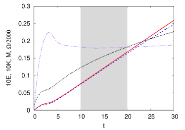
Figure 1: Time evolution of the total energy $E$ (red solid line), kinetic energy $K$ (blue dashed line), enstrophy $\Omega$ (purple dash-dotted line), and Mach number $M$ (black dotted line). The values of $E$ and $K$ have been multiplied by a factor of 10, and $\Omega$ by a factor of $1/2000$ for plotting purposes.

In contrast to the energy, we find that after an initial growth, the enstrophy $\Omega$ reaches an almost constant value (see Fig. 1). This happens because the direct enstrophy cascade transfers the enstrophy injected by the forcing to the small scales, where it is removed by numerical dissipation.

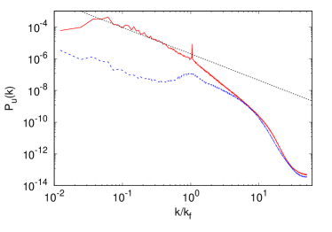
Figure 2: Power spectra of the solenoidal component of the velocity $P_{s}(k)$ (red solid line) and of the irrotational component $P_{i}(k)$ (blue dashed line), at time $t=20$. Black dotted line represents Kolmogorov scaling $k^{-5/3}$.

At late times, the inverse energy cascade will eventually produce an accumulation of the energy at the largest scale, giving rise to the formation of an intense vortex dipole (the condensate). The formation of this vortical structure results in non-Gaussian statistics in the vorticity field and causes the breaking of scale invariance Kritsuk (2019). Considering that we are interested in the study of the conformal invariance of the vorticity field, it is crucial to verify that the field is at least scale-invariant. For this reason, in the following we will limit our analysis to the time range $10<t<20$, i.e., well before the beginning of the formation of the condensate. Moreover, in this time interval the value of $\Omega$ is almost constant, which allows us to assume that the dynamics of the vorticity field are in a statistically steady state. In this time range, the Mach number varies from $M\simeq 0.12$ at $t=10$ to $M\simeq 0.18$ at $t=20$ (Fig. 1). The dynamics are therefore weakly compressible.

Furthermore, we will consider the scaling properties in the range of scales of the inverse cascade $L_{f}\ll r\ll L$, in which the conformal invariance has been detected for the case of 2D incompressible turbulence Bernard et al. (2006). As shown in Figure 2, in the range of wavenumbers of the inverse cascade ($0.04k_{f}<k<k_{f}$) the power spectrum of kinetic energy is dominated by the spectrum of the solenoidal component of the velocity field $P_{s}(k)=\sum_{|q|=k}|{\bm{u}}_{s}(q)|^{2}$, while the spectrum of the irrotational component $P_{i}(k)=\sum_{|q|=k}|{\bm{u}}_{i}(q)|^{2}$ is much smaller (by more than a factor of $200$ between $0.04k_{f}<k<0.4k_{f}$). The power spectrum of the solenoidal component $P_{s}(k)$ displays an approximatively Kolmogorov slope for wavenumbers $k<0.6k_{f}$ with a steeper exponent close to $-2$ close to the forcing scale Falkovich and Kritsuk (2017); Kritsuk (2019). At high wavenumbers, the spectra of the irrotational and solenoidal components become comparable. With a more accurate numerical method and adaptively controlled numerical dissipation, two independent direct cascades can be resolved at $k>k_{f}$: the enstrophy cascade and the acoustic energy cascade. These are reflected in the scaling of power spectra, $P_{s}(k)\sim k^{-3}\ln{(k/k_{f})}$ and $P_{i}(k)\sim k^{-2}$ Kritsuk (2019). While $P_{s}(k)$ dominates at $k\lesssim k_{f}$, $P_{i}(k)$ inevitably becomes dominant at $k\gg k_{f}$.

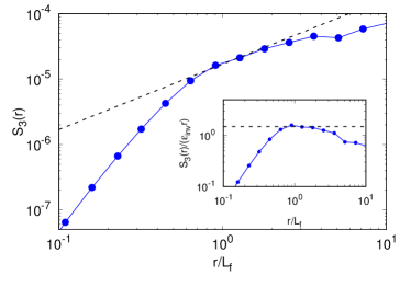
Figure 3: Third-order longitudinal structure function $S_{3}(r)$ (blue circles) average over times $10\leq t\leq 20$. Black dashed line represents (6). Inset: compensated structure function $S_{3}(r)/(\varepsilon_{inv}r)$ (blue circles) and the predicted value $3/2$ (black dashed line).

Another indication of the scale invariance of the velocity field in the range of scales of the inverse energy cascade is provided by the third-order longitudinal structure function (SF) $S_{3}(r)=\langle(\delta u_{L}(r))^{3}\rangle$ where $\delta u_{L}(r)=[{\bm{u}}({\bm{x}}+{\bm{r}})-{\bm{u}}({\bm{x}})]\cdot{\bm{r}}/r$ is the longitudinal velocity difference at scale $r$. In 2D incompressible turbulence, the constant energy flux in the inertial range gives an exact prediction for the third-order structure function which, in homogeneous and isotropic conditions reads Bernard (1999); Lindborg (1999)

$$S_{3}(r)={3\over 2}\varepsilon_{inv}r,$$ (6)

where $\varepsilon_{inv}$ represent the inverse kinetic energy flux. The third-order SF, time averaged for $10<t<20$ in our simulation, is shown in Figure 3. It displays a linear scaling range at $r>L_{f}$ with a coefficient ${3\over 2}\varepsilon_{inv}$ (see inset of Fig. 3) in agreement with the assumption of a constant energy flux. Let us notice that, because of the lack of stationarity at large scales $r\gg L_{f}$, the scaling $S_{3}(r)\sim r$ is observed only in a narrow range of scales.

IV Conformal invariance of isovorticity lines

The discovery of conformal invariance in two-dimensional turbulence was first made for the zero-vorticity lines in incompressible Navier-Stokes equations Bernard et al. (2006) and then extended to others two-dimensional turbulent systems characterized by different scaling laws Bernard et al. (2007); Falkovich and Musacchio (2010). These previous results suggest the possibility to also test conformal invariance in the inverse cascade of weakly compressible turbulence.

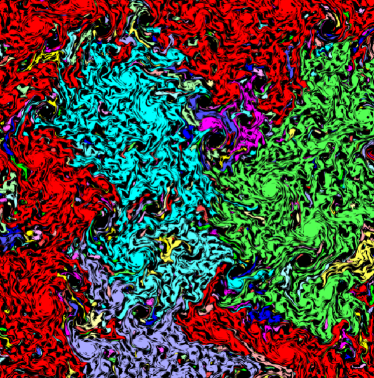
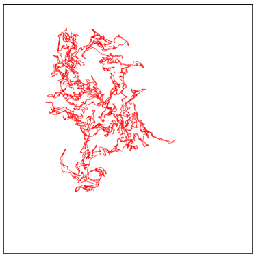
Figure 4: Top: Vorticity cluster, defined as connected regions with the same sign of vorticity (here positive). Different colors are attributed to different clusters. Regions of negative vorticity are black. Bottom: Zero-vorticity isoline of the cyan cluster.

We have extracted the vorticity clusters (i.e. connected regions of positive/negative vorticity) and zero vorticity isolines (boundaries of vorticity clusters) from the different fields of the simulation. We have obtained an ensemble of $N_{c}=461,399$ clusters. One example of these clusters is shown in Fig. 4 for an intermediate time in the simulation $t=20$. Here, we observe the presence of clusters of different sizes, each one enclosed by a complex, fractal boundary.

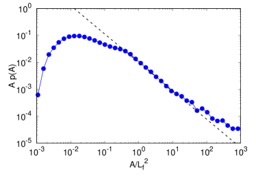
Figure 5: Probability density function of cluster size $A$ (blue circles). The black dashed line represents the scaling prediction by percolation theory $Ap(A)\sim A^{-96/91}$.

Figure 5 shows the probability distribution function (PDF) $p(A)$ of cluster size $A$, defined as the number of connected sites which belong to the cluster. The PDF displays a power-law behavior in the range $L_{f}^{2}<A<10L_{f}^{2}$. The scaling exponent observed in Fig. 5 is in agreement with the theoretical value predicted in the case of critical percolation in 2D $p(A)\sim A^{-96/91-1}$. Stauffer and Aharony (2018) The same value has been previously observed for the scaling exponent of the PDF of vorticity clusters size in the case of incompressible 2D Navier-Stokes Bernard et al. (2006).

This result suggests that vorticity clusters produced by the inverse cascade in weakly compressible turbulence are statistically equivalent to clusters of critical percolation and therefore display the same properties of conformal invariance. In particular, the cluster boundaries in the continuous limit are expected to belong to the class of conformal curves called SLE curves Schramm (2000); Cardy (2005). In order to introduce briefly the basics of the SLE, let us consider a curve $\gamma(s)$, parameterized by the time $s$, starting from a point of the boundary of the half-plane $H$. At given time $s$, the curve $\gamma(s)$ define a region $K_{s}$ (the hull) formed by the points of the complex half-plane which cannot be reached from infinity without crossing the curve, plus the curve itself. The simply connected set $H\setminus K_{s}$ can be mapped into $H$ by an analytic function $g_{s}(z)$ which satisfies the asymptotic behavior $g_{s}(z)\sim z+2s/z+O(z^{-2})$ at $z\to\infty$. The conformal map $g_{s}(z)$ obeys the differential Löwner equation Löwner (1923):

$$\frac{dg_{s}}{ds}=\frac{2}{g_{s}(z)-\xi(s)},$$ (7)

where $\xi(s)$ is the real driving function. The Löwner equation establishes an equivalence between the curve $\gamma(s)$ and its driving function $\xi(s)$. Different driving functions produce different curves. In the case of random curves $\gamma(s)$, the equation (7) is called stochastic Loewner evolution (SLE) and the driving $\xi(s)$ is a random real variable. It has been demonstrated that the statistics of random curves are conformal invariant if and only if the driving is a Brownian walk, i.e. a random function with independent increments and with $\langle(\xi(s)-\xi(0))^{2}\rangle=\kappa s$. Here, $\kappa$ is the diffusion coefficient which classifies the universality class of cluster boundaries in critical phenomena in 2D Bauer and Bernard (2003); Gruzberg and Kadanoff (2004); Cardy (2005). One of the predictions for SLE curves is their fractal dimension, which is known to be $D=1+\kappa/8$ (for $\kappa<8$). In the case of critical percolation, for which $\kappa=6$, the prediction is $D=7/4$ which has been indeed measured in the vorticity cluster of two-dimensional turbulenceBernard et al. (2006).

We have therefore extracted the zero-vorticity line from the fields of weakly compressible turbulence. The extraction is performed by means of an algorithm which follows the frontier of a cluster of vorticity by always keeping the positive region on the right of the path. At variance with “true” SLE curves, in our numerical simulation, scale (and conformal) invariance can be expected in the range of scales of the inverse cascade only. Therefore, for numerical convenience, we have coarse-grained the vorticity fields produced by the simulation by halving the resolution to a $4096\times 4096$ grid. One example of vorticity isoline obtained from this procedure is shown in Fig. 4 (right panel). The total number of isolines obtained is $N=1144$.

We have computed the correlation dimension $D_{2}$ of the zero-vorticity isolines by computing the probability density function (PDF) $p(R)$ of finding two points belonging to the same isoline at distance $R$. For a fractal set, the probability scales as $p(R)\propto R^{D_{2}-1}$. As shown in Fig. 6, the PDF $p(R)$ displays a scaling exponent in agreement with the prediction for the SLE curves with $\kappa=6$, i.e., $D_{2}=7/4$ in the range of scales $1\lesssim R/L_{f}\lesssim 7$, which corresponds to the the inverse cascade.

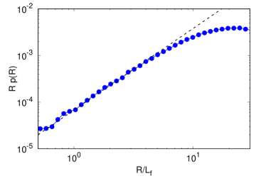
Figure 6: Probability density function of distances $R$ between two points belonging to the the same zero-vorticity line (blue circles). The black dashed line represents the theoretical prediction $Rp(R)\sim R^{7/4}$.

Assuming that the ensemble of zero-vorticity isolines is statistically equivalent to SLE curves, we have derived the associated ensemble of driving functions $\xi(s)$. The algorithm which computes the driving for a generic curve is based on the solution of the Eq. (7) in the case of an infinitesimal line segment starting from the origin $(0,0)$ and ending in $(\xi,2\sqrt{ds})$: $g_{ds}(z)=\xi+\sqrt{(z-\xi)^{2}+4ds}$. By approximating the generic curve $\gamma(s)$ with piecewise line segments, one obtains the associated driving function $\xi(s)$ (see Bernard et al. (2006) for further details). Averaging over the ensemble of $N=1144$ driving functions obtained, we have computed the variance $\sigma^{2}_{\xi}=\langle(\xi(s)-\langle\xi(s)\rangle)^{2}\rangle$. In the range $1\lesssim s/(2L_{f})^{2}\lesssim 7$, we find that the variance grows linearly as $\sigma^{2}_{\xi}=\kappa s$ (see Fig.7). The driving $\xi(s)$ is therefore a diffusive process with $\kappa\approx(5.7\pm 0.2)$, which is close (within the statistical uncertainty) to the expected value of $\kappa=6$. Moreover, the PDF of the standardized driving $(\xi(s)-\langle\xi(s)\rangle)/(\kappa s)^{1/2}$ collapses onto a standard Gaussian distribution function for values of $s$ in the scaling range (see Fig. 8). These findings support the conjecture that the driving function is a genuine Brownian motion $\xi_{s}=\sqrt{\kappa}B_{s}$, and that the vorticity isolines are SLE-curves belonging to the same class of universality of percolation corresponding to $\kappa=6$.

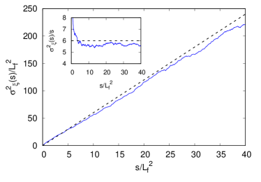
Figure 7: Variance of driving function$\sigma^{2}_{\xi}(s)$ as a function of the parameterization $s$ (blue solid line) and the theoretical prediction $\sigma^{2}_{\xi}(s)=\kappa s$ with $\kappa=6$ (black dashed line). In the inset we show the compensated value $\sigma^{2}_{\xi}(s)/s$.

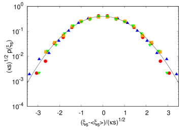
Figure 8: PDF of the driving functions $\xi_{s}$ at different values of $s$: $s=10L_{f}^{2}$ (blue upper triangles), $s=20L_{f}^{2}$ (red circles), $s=30L_{f}^{2}$ (orange squares), $s=40L_{f}^{2}$ (green lower triangles).

V Conclusions

In this work we have studied the conformal invariance of weakly compressible two-dimensional turbulence. We have shown that the isolines of vorticity clusters are compatible with SLE curves in the universality class of critical percolation, as in the case of incompressible two-dimensional turbulence. Our results therefore extend those obtained in others two-dimensional turbulent systems (Navier-Stokes, surface quasi-geostrophic, Charney-Hasegawa-Mima) to the realm of (weakly) compressible turbulence.

One question which naturally arises from our results is whether the conformal invariance property would survive in higher compressible regimes characterized by larger Mach numbers. While this is in principle interesting, we remark that, by increasing the Mach number, a different phenomenology emerges at large scales: when velocity fluctuations reach the speed of sound, kinetic energy produces shock waves which arrest the inverse cascade and provide a new mechanism of energy dissipation Falkovich and Kritsuk (2017). This “flux loop” introduces a characteristic scale in the process which breaks the scaling invariance of the cascade. Conformal (and scaling) invariance could still survive in the limited range of scales between energy injection and shock wave production, and its study would be an interesting problem for future investigation.