A simple computational approach to the Susceptible-Infected-Recovered (SIR) epidemic model via the Laplace-Adomian Decomposition Method

Abstract

The Susceptible-Infected-Recovered (SIR) epidemic model is extensively used for the study of the spread of infectious diseases. Even that the exact solution of the model can be obtained in an exact parametric form, in order to perform the comparison with the epidemiological data a simple but highly accurate representation of the time evolution of the SIR compartments would be very useful. In the present paper we obtain a series representation of the solution of the SIR model by using the Laplace-Adomian Decomposition Method to solve the basic evolution equation of the model. The solutions are expressed in the form of infinite series. The series representations of the time evolution of the SIR compartments are compared with the exact numerical solutions of the model. We find that there is a good agreement between the Laplace-Adomian semianalytical solutions containing only three terms, and the numerical results.

Keywords: Susceptible-Infected-Recovered (SIR) epidemic model; Laplace-Adomian Decomposition Method; series solution

I Introduction

The major Covid-19 coronavirus pandemic that began in 2019 in Wuhan, China China , has again underlined the necessity of understanding on both quantitative and qualitative levels the outbreak and spread of infectious diseases. This problem has been already studied a long time ago, John Graunt being the first scientist who attempted to evaluate in a methodical way the causes of fatalities during epidemics 1 . His analysis led to a theory that is still widely accepted by the modern epidemiologists. The first mathematician who did propose a mathematical model describing the dynamics of an infectious disease was Daniel Bernoulli, who modeled the spread of Variola, which was rampant at the time, in 1760 Ber1 . Moreover, in a later study Daniel Bernoulli did present the advantages of inoculation Ber2 , the method first used to immunize an individual against smallpox with material taken from a patient.

More recently an important simple (compartmental) deterministic model predicting the spread of epidemic outbreaks was proposed by McKendrick and Kermack in 1927 2 . This mathematical epidemic model is called the Susceptible-Infected-Recovered (SIR) model, or the $xyz$ model. In the SIR model it is assumed that in the presence of an infectious disease a population with a fixed number can be compartmentalized into three groups (compartments), denoted (S), (I) and (R), respectively. More precisely, the compartments used in the McKendrick-Kermack model are defined as follows 2 :

a) The (S) (susceptible) compartment consists of the individuals in the total population not yet infected with the disease at time $t$, or those susceptible to the disease. The number of individuals in this compartment is denoted $x(t)$.

b) The (I) (infected) compartment consists of the individuals who have been infected with the epidemic disease, and who can spread the disease to those in the susceptible category. The number of individuals in the (I) compartment is denoted $y\left(t\right)$.

c) The (R) (recovered) compartment consists of the individuals who have been infected during the epidemics, and did fully recover. The individuals in the (R) compartment, whose number is denoted by $z(t)$, cannot be infected again, and they are not able to transmit the disease to others.

From a mathematical point of view the SIR model is formulated in terms of a strongly nonlinear system of ordinary differential equations. The behavior of the SIR model essentially depends on two constants $\beta$ and $\gamma$ that give the transition rates between compartments.

The transition rate between the S (Susceptible) and I (infected) groups is denoted by $\beta$. It represents the contact rate, that is, the probability of being infected when the contact between a susceptible and an infectious individual takes place 14 ; Mur ; 15 ; Mur1 .

The transition rate between the I (Infected) and R (recovered) compartments is denoted by $\gamma$. $\gamma$ gives the rate of recovery or death. If we denote by $D$ the total duration of the infection, then $\gamma=1/D$, expressing the fact that an individual experiences one recovery in $D$ units of time 14 ; Mur ; 15 ; Mur1 . Since in the SIR model both $\beta$ and $\gamma$ represent transition rates (probabilities), their range of values is $0\leq\beta\leq 1$ and $0\leq\gamma\leq 1$, respectively.

The SIR model has been investigated from both mathematical and epidemiological point of view in a large number of studies. Its exact solution has been obtained in a parametric form in Harko1 . The SIR model has been used extensively for the simulation of the dynamics of the Covid-19 pandemic and its impact on society Cov1 ; Cov2 ; Cov3 ; Cov4 ; Cov5 ; Cov6 ; Cov7 ; Cov8 ; Cov9 ; Cov10 ; Cov11 . Despite the large number of mathematical and numerical investigations of the SIR model, including the use of the Adomian decomposition method 5 , of the variational iteration method 6 , of the homotopy perturbation method 7 , and of the differential transformation method 8 , a simple but precise representation of the solution of the SIR model that could be efficiently used in epidemiological and populations studies is still missing.

It is the purpose of this work to present a simple series solution of the SIR epidemic model. To achieve this goal we first derive the basic equation of the SIR model, which is represented by a first order nonlinear differential equation for $z(t)$. Even that this equation can be solved exactly, in a parametric form, we will investigate it by using the Laplace-Adomian Decomposition Method (LADM), which is an extension of the standard Adomian Decomposition Method Ad1 ; Ad2 ; Ad3 . The ADM is a powerful mathematical method that permit to find semianalytical solutions of different types of ordinary, partial and integral differential nonlinear equations. The ADM allows to obtain the solution of a differential equation in the form of a series, with the terms of the series determined recursively by using the Adomian polynomials Ad1 ; Ad2 . The Laplace-Adomian Method has been used to investigate nonlinear differential equations in different fields of science in Ad4 ; Ad5 ; Ad6 ; Ad7 ; Ad8 ; Ad9 ; Ad10 . By applying the Laplace-Adomian Method to the basic equation of the SIR model its solution can be represented as a series that gives an excellent description of the numerical results.

The present paper is organized as follows. The series solution of the SIR epidemic model is obtained in Section II, where its comparison with the exact numerical solution is also performed. We briefly conclude our results in Section III.

II Series solution of the SIR epidemic model

In the present Section we will present a semianalytical solution of the SIR model represented in the form of a series containing exponential terms. The basic equations of the SIR model are

$$\frac{dx}{dt}=-\beta x\left(t\right)y\left(t\right),$$ (1)

$$\frac{dy}{dt}=\beta x\left(t\right)y\left(t\right)-\gamma y\left(t\right),$$ (2)

and

$$\frac{dz}{dt}=\gamma y\left(t\right),$$ (3)

respectively, where $x(t)>0$, $y(t)>0$ and $z(t)>0$, $\forall t\geq 0$. The system of equations (1)-(3) must be integrated with the initial conditions $x\left(0\right)=N_{1}\geq 0$, $y\left(0\right)=N_{2}\geq 0$ and $z\left(0\right)=N_{3}\geq 0$, respectively, where $N_{i}\in\Re$, $i=1,2,3$. The time evolution of the model is determined by two epidemiological parameters, the infection rate $\beta$, and the mean recovery rate $\gamma$, which in the following are assumed to be positive constants.

By adding Eqs. (1)–(3) we immediately obtain the differential equation,

$$\frac{d}{dt}\left[x(t)+y(t)+z(t)\right]=0,$$ (4)

which upon integration gives the first integral of the SIR system

$$x(t)+y(t)+z(t)=N,\forall t\geq 0,$$ (5)

Hence it follows that in this epidemiological model the total size of the population $N=\sum_{i=1}^{3}{N_{i}}$ is, from a mathematical point of view, an arbitrary positive integration constant. This result is consistent with our assumption of considering only three compartments in a fixed population with $N$ members.

II.1 The basic evolution equation for the SIR model

We will now show that the SIR model can be equivalently formulated in terms of a first order nonlinear differential equation. After differentiating Eq. (1) with respect to the time $t$ we obtain the following second order differential equation,

$$\frac{dy}{dt}=-\frac{1}{\beta}\left[\frac{x^{\prime\prime}}{x}-\left(\frac{x^{\prime}}{x}\right)^{2}\right],$$ (6)

where in the following we denote by a prime the derivative with respect to time $t$. By inserting Eqs. (1) and (6) into Eq. (2), we obtain

$$\frac{x^{\prime\prime}}{x}-\left(\frac{x^{\prime}}{x}\right)^{2}+\gamma\frac{x^{\prime}}{x}-\beta x^{\prime}=0.$$ (7)

From Eqs. (1) and (3) we find the evolution equation for $z$, in terms of $x$ as

$$\frac{dz}{dt}=-\frac{\gamma}{\beta}\left(\frac{x^{\prime}}{x}\right)\,.$$ (8)

which can be integrated to give

$$x=x_{0}e^{-(\beta/\gamma)z},$$ (9)

The value of the positive integration constant $x_{0}$ can be obtained from the initial conditions of the SIR model as

$$x_{0}=N_{1}e^{(\beta/\gamma)N_{3}}.$$ (10)

With the use of Eq. (7), Eq. (6) becomes

$$\frac{dy}{dt}=-x^{\prime}+\frac{\gamma}{\beta}\frac{x^{\prime}}{x},$$ (11)

immediately giving

$$y(t)=\frac{\gamma}{\beta}\ln x-x+C_{1},$$ (12)

where $C_{1}$ is an arbitrary integration constant, which can be determined from the initial conditions as

$$C_{1}=N_{1}+N_{2}-\frac{\gamma}{\beta}\ln N_{1}.$$ (13)

After differentiating Eqs. (9) and (8) with respect to the time $t$, we obtain the basic second order differential equation for $z(t)$, describing the spread of the non-fatal disease in a given population,

$$z^{\prime\prime}=x_{0}\beta z^{\prime}e^{-\frac{\beta}{\gamma}z}-\gamma z^{\prime}.$$ (14)

Eq. (14), a strongly nonlinear differential equation, is mathematically equivalent to the first order system of differential equations Eqs. (1)–(3), respectively, giving the SIR epidemic model. However, a first order nonlinear differential equation can also de obtained to describe the evolution of $z$. Eq. (14) can be rewritten as

$$\frac{d^{2}z}{dt^{2}}+\gamma\frac{dz}{dt}=-\gamma x_{0}\frac{d}{dt}e^{-(\beta/\gamma)z},$$ (15)

and thus we obtain its first integral as given by

$$\frac{dz}{dt}+\gamma z=-\gamma x_{0}e^{-(\beta/\gamma)z}+C,$$ (16)

where $C$ is an arbitrary constant of integration. By estimating the above equation at $t=0$ and with the help of Eq. (3) we obtain the value of the integration constant as

$$C=\gamma\left(N_{2}+N_{3}\right)+\gamma x_{0}e^{-\frac{\beta}{\gamma}N_{3}}=\gamma N.$$ (17)

II.2 Series solution of the basic equation of the SIR model via the Laplace-Adomian method

The general solution of Eq. (16) can be obtained in a closed form, in an exact parametric representation. However, the parametric representation is not particularly useful from a computational point of view. That’s why in the following we will obtain a series solution of Eq. (16). In order to do this we will use the Laplace-Adomian method.

In the Laplace-Adomian method we first apply the Laplace transformation operator $\mathcal{L}_{x}$, defined as $\mathcal{L}_{x}[f(x)](s)=\int_{0}^{\infty}{f(x)e^{-sx}dx}$, to Eq. (16), thus obtaining

$$\mathcal{L}_{t}\left[\frac{dz(t)}{dt}\right](s)+\gamma\mathcal{L}_{t}[z(t)](s)-\mathcal{L}_{t}[C](s)=-\gamma x_{0}\mathcal{L}_{t}\left[e^{-(\beta/\gamma)z(t)}\right](s).$$ (18)

By using the properties of the Laplace transform we immediately find

$$(\gamma+s)\mathcal{L}_{t}[z(t)](s)-\frac{\gamma N+sz(0)}{s}=-\gamma x_{0}\mathcal{L}_{t}\left[e^{-(\beta/\gamma)z(t)}\right](s).$$ (19)

With the use of the initial condition $z(0)=N_{3}$ we obtain

$$\mathcal{L}_{t}[z(t)](s)=\frac{\gamma N+N_{3}s}{s(\gamma+s)}-\frac{\gamma x_{0}}{\gamma+s}\mathcal{L}_{t}\left[e^{-(\beta/\gamma)z(t)}\right](s).$$ (20)

We assume now that the function $z(t)$ can be represented in the form of an infinite series,

$$z(t)=\sum_{n=0}^{\infty}z_{n}(t),$$ (21)

where the terms $z_{n}(t)$ can be computed recursively. As for the nonlinear operator $f(z(t))=-\gamma x_{0}e^{-(\beta/\gamma)z(t)}$, we assume that it can be decomposed as

$$f(z(t))=-\gamma x_{0}e^{-(\beta/\gamma)z(t)}=\sum_{n=0}^{\infty}A_{n}(t),$$ (22)

where the $A_{n}$’s are Adomian polynomials, defined generally for an arbitrary function $f(z(t))$ according to Ad3

$$A_{n}=\left.\frac{1}{n!}\frac{d^{n}}{d\lambda^{n}}f\left(\sum_{i=0}^{\infty}{\lambda^{i}z_{i}}\right)\right|_{\lambda=0}.$$ (23)

The first five Adomian polynomials can be obtained in the following form,

$$A_{0}=f\left(z_{0}\right),$$ (24)

$$A_{1}=z_{1}f^{\prime}\left(z_{0}\right),$$ (25)

$$A_{2}=z_{2}f^{\prime}\left(z_{0}\right)+\frac{1}{2}z_{1}^{2}f^{\prime\prime}\left(z_{0}\right),$$ (26)

$$A_{3}=z_{3}f^{\prime}\left(z_{0}\right)+z_{1}z_{2}f^{\prime\prime}\left(z_{0}\right)+\frac{1}{6}z_{1}^{3}f^{\prime\prime\prime}\left(z_{0}\right),$$ (27)

$$A_{4}=z_{4}f^{\prime}\left(z_{0}\right)+\left[\frac{1}{2!}z_{2}^{2}+z_{1}z_{3}\right]f^{\prime\prime}\left(z_{0}\right)+\frac{1}{2!}z_{1}^{2}z_{2}f^{\prime\prime\prime}\left(z_{0}\right)+\frac{1}{4!}z_{1}^{4}f^{(\mathrm{iv})}\left(z_{0}\right).$$ (28)

Substituting Eqs. (21) and (22) into Eq. (20) we obtain

$$\mathcal{L}_{t}\left[\sum_{n=0}^{\infty}z_{n}(t)\right]=\frac{\gamma N+N_{3}s}{s(\gamma+s)}-\frac{1}{\gamma+s}\mathcal{L}_{t}[\sum_{n=0}^{\infty}A_{n}].$$ (29)

The matching of both sides of Eq. (29) gives the following iterative algorithm for the power series solution of the basic evolution equation of the SIR model, Eq. (16),

$$\mathcal{L}_{t}\left[z_{0}(t)\right](s)=\frac{\gamma N+N_{3}s}{s(\gamma+s)},$$ (30)

$$\mathcal{L}_{t}\left[z_{1}(t)\right](s)=-\frac{1}{\gamma+s}\mathcal{L}_{t}\left[A_{0}(t)\right](s),$$ (31)

$$\mathcal{L}_{t}\left[z_{2}(t)\right](s)=-\frac{1}{s+\gamma}\mathcal{L}_{t}\left[A_{1}(t)\right](s),$$ (32)

$$...$$

$$\mathcal{L}_{t}\left[z_{k+1}(t)\right](s)=-\frac{1}{s+\gamma}\mathcal{L}_{t}\left[A_{k}(t)\right](s).$$ (33)

By applying the inverse Laplace transformation to Eq. (30), we obtain the value of $z_{0}$ as

$$z_{0}(t)=\mathcal{L}_{t}^{-1}\left\{\left[\frac{\gamma N+N_{3}s}{s(\gamma+s)}\right](s)\right\}(t)=N-\left(N_{1}+N_{2}\right)e^{-\gamma t}.$$ (34)

In the following, for computational simplicity, we will approximate $z_{0}(t)$ by its first order series expansion, given by

$$z_{0}(t)\approx N_{3}+\gamma\left(N_{1}+N_{2}\right)t.$$ (35)

The first Adomian polynomial is given by $A_{0}(t)=-\gamma x_{0}e^{-(\beta/\gamma)z_{0}(t)}$, and thus, within the adopted approximation, we obtain

$$A_{0}(t)=-\gamma N_{1}e^{-\beta\left(N_{1}+N_{2}\right)t},$$ (36)

and

$$z_{1}(t)=-\mathcal{L}_{t}^{-1}\left\{\frac{1}{s+\gamma}\mathcal{L}_{t}\left[\gamma N_{1}e^{-\beta\left(N_{1}+N_{2}\right)t}\right](s)\right\}(t)=\frac{\gamma N_{1}\left[e^{-\beta\left(N_{1}+N_{2}\right)t}-e^{-\gamma t}\right]}{\beta\left(N_{1}+N_{2}\right)-\gamma},$$ (37)

respectively. The second Adomian polynomial is obtained as

$$A_{1}(t)=-\frac{\beta\gamma N_{1}^{2}e^{-\left[\gamma+2\beta\left(N_{1}+N_{2}\right)\right]t}\left[e^{\beta\left(N_{1}+N_{2}\right)t}-e^{\gamma t}\right]}{\beta\left(N_{1}+N_{2}\right)-\gamma},$$ (38)

and thus we find

$$z_{2}(t)=\mathcal{L}_{t}^{-1}\left\{\frac{1}{s+\gamma}\mathcal{L}_{t}\left[A_{1}(t)\right](s)\right\}(t)=$$

$$\frac{\gamma N_{1}^{2}e^{-\left[\gamma+2\beta\left(N_{1}+N_{2}\right)\right]t}\left\{-\beta\left(N_{1}+N_{2}\right)e^{\gamma t}+\left[2\beta\left(N_{1}+N_{2}\right)-\gamma\right]e^{\beta\left(N_{1}+N_{2}\right)t}+\left[\gamma-\beta\left(N_{1}+N_{2}\right)\right]e^{2\beta\left(N_{1}+N_{2}\right)t}\right\}}{\left(N_{1}+N_{2}\right)\left[\beta\left(N_{1}+N_{2}\right)-\gamma\right]\left[2\beta\left(N_{1}+N_{2}\right)-\gamma\right]}.$$ (39)

Similarly, after computing the third Adomian polynomial, we obtain

$$z_{3}(t) = \frac{\gamma N_{1}^{3}}{2\left[\gamma-\beta\left(N_{1}+N_{2}\right)\right]^{2}}\Bigg{\{}\frac{\beta^{2}\left[4\beta\left(N_{1}+N_{2}\right)-3\gamma\right]e^{-3\beta\left(N_{1}+N_{2}\right)t}}{\gamma^{2}+6\beta^{2}\left(N_{1}+N_{2}\right)^{2}-5\beta\gamma\left(N_{1}+N_{2}\right)}+\frac{\beta^{2}e^{-\left[2\gamma+\beta\left(N_{1}+N_{2}\right)\right]t}}{\gamma+\beta\left(N_{1}+N_{2}\right)}+$$ (40)

$$\frac{2\left[\gamma-\beta\left(N_{1}+N_{2}\right)\right]^{2}e^{-\left[\gamma+\beta\left(N_{1}+N_{2}\right)\right]t}}{\left(N_{1}+N_{2}\right)^{2}\left[2\beta\left(N_{1}+N_{2}\right)-\gamma\right]}+\frac{\left[\gamma-2\beta\left(N_{1}+N_{2}\right)\right]e^{-\left[\gamma+2\beta\left(N_{1}+N_{2}\right)\right]t}}{\left(N_{1}+N_{2}\right)^{2}}-$$

$$\frac{e^{-\gamma t}\left[\gamma-\beta\left(N_{1}+N_{2}\right)\right]^{2}\left[\gamma+2\beta(N_{1}+N_{2})\right]}{\left(N_{1}+N_{2}\right)^{2}\left[3\beta\left(N_{1}+N_{2}\right)-\gamma\right]\left[\gamma+\beta\left(N_{1}+N_{2}\right)\right]}\Bigg{\}}.$$

Finally, we will present the $z_{4}(t)$ term in the Adomian series expansion, which is given by

$$z_{4}(t) = \frac{1}{6}\gamma N_{1}^{4}\Bigg{\{}\frac{2\beta^{3}\left[8\gamma-9\beta\left(N_{1}+N_{2}\right)\right]e^{-4\beta\left(N_{1}+N_{2}\right)t}}{\left[\beta\left(N_{1}+N_{2}\right)-\gamma\right]^{3}\left[3\beta\left(N_{1}+N_{2}\right)-\gamma\right]\left[4\beta\left(N_{1}+N_{2}\right)-\gamma\right]}+$$ (41)

$$\frac{\beta^{3}e^{-\left[3\gamma+\beta\left(N_{1}+N_{2}\right)\right]t}}{\left[\beta\left(N_{1}+N_{2}\right)-\gamma\right]^{3}\left[2\gamma+\beta\left(N_{1}+N_{2}\right)\right]}+$$

$$\frac{6\beta^{2}\left[\gamma^{2}-2\beta^{2}\left(N_{1}+N_{2}\right)^{2}\right]e^{-2\left[\gamma+\beta\left(N_{1}+N_{2}\right)\right]t}}{\left(N_{1}+N_{2}\right)\left[\beta\left(N_{1}+N_{2}\right)-\gamma\right]^{3}\left[\gamma+\beta\left(N_{1}+N_{2}\right)\right]\left[\gamma+2\beta\left(N_{1}+N_{2}\right)\right]}+$$

$$\frac{6\beta^{2}e^{-\left[2\gamma+\beta\left(N_{1}+N_{2}\right)\right]t}}{\left(N_{1}+N_{2}\right)\left[\beta\left(N_{1}+N_{2}\right)-\gamma\right]\left[2\beta\left(N_{1}+N_{2}\right)-\gamma\right]\left[\gamma+\beta\left(N_{1}+N_{2}\right)\right]}+$$

$$\frac{e^{-\gamma t}\left[-2\gamma^{3}-12\beta^{3}\left(N_{1}+N_{2}\right)^{3}-28\beta^{2}\gamma\left(N_{1}+N_{2}\right)^{2}-13\beta\gamma^{2}\left(N_{1}+N_{2}\right)\right]}{\left(N_{1}+N_{2}\right)^{3}\left[4\beta\left(N_{1}+N_{2}\right)-\gamma\right]\left[\gamma+\beta\left(N_{1}+N_{2}\right)\right]\left[\gamma+2\beta\left(N_{1}+N_{2}\right)\right]\left[2\gamma+\beta\left(N_{1}+N_{2}\right)\right]}+$$

$$\frac{\left[-\gamma^{3}+12\beta^{3}\left(N_{1}+N_{2}\right)^{3}-17\beta^{2}\gamma\left(N_{1}+N_{2}\right)^{2}+7\beta\gamma^{2}\left(N_{1}+N_{2}\right)\right]e^{-\left[\gamma+3\beta\left(N_{1}+N_{2}\right)\right]t}}{\left(N_{1}+N_{2}\right)^{3}\left[\beta\left(N_{1}+N_{2}\right)-\gamma\right]^{3}\left[2\beta\left(N_{1}+N_{2}\right)-\gamma\right]}+$$

$$\frac{\left[3\gamma+6\beta\left(N_{1}+N_{2}\right)\right]e^{-\left[\gamma+\beta\left(N_{1}+N_{2}\right)\right]t}}{\left(N_{1}+N_{2}\right)^{3}\left[3\beta\left(N_{1}+N_{2}\right)-\gamma\right]\left[\gamma+\beta\left(N_{1}+N_{2}\right)\right]}-\frac{3e^{-\left[\gamma+2\beta\left(N_{1}+N_{2}\right)\right]t}}{\left(N_{1}+N_{2}\right)^{3}\left[\beta\left(N_{1}+N_{2}\right)-\gamma\right]}\Bigg{\}}.$$

The higher order terms in the Laplace-Adomian power series representation of $z(t)$ can be easily obtained with the help of some symbolic computation software. Hence, the solution of the SIR system can be obtained as

$$x(t)=x_{0}e^{-\frac{\beta}{\gamma}\sum_{i=0}^{\infty}{z_{i}(t)}}=N_{1}e^{(\beta/\gamma)\left(N_{3}-\sum_{i=0}^{\infty}{z_{i}(t)}\right)},$$ (42)

$$y(t) = N_{1}+N_{2}+\frac{\gamma}{\beta}\ln\frac{x_{0}e^{-\frac{\beta}{\gamma}\sum_{i=0}^{n}{z_{i}(t)}}}{N_{1}}-x_{0}e^{-\frac{\beta}{\gamma}\sum_{i=0}^{n}{z_{i}(t)}}=$$ (43)

$$N_{1}+N_{2}+N_{3}-\sum_{i=0}^{\infty}{z_{i}(t)}-N_{1}e^{(\beta/\gamma)\left(N_{3}-\sum_{i=0}^{\infty}{z_{i}(t)}\right)},$$

and

$$z(t)=\sum_{i=0}^{\infty}{z_{i}(t)},$$ (44)

respectively.

II.3 Comparison with the exact numerical solution

In order to test the applicability of the power series solutions solving the SIR model we will compare the truncated Laplace-Adomian series with the exact numerical solution. To perform the comparison we will consider only the first three terms in the expansion of $z$, so that $z(t)\approx z_{0}(t)+z_{1}(t)+z_{2}(t)$, or, explicitly,

$$z(t) \approx N-\left(N_{1}+N_{2}\right)e^{-\gamma t}+\frac{\gamma N_{1}\left[e^{-\beta\left(N_{1}+N_{2}\right)t}-e^{-\gamma t}\right]}{\beta\left(N_{1}+N_{2}\right)-\gamma}+\gamma N_{1}^{2}e^{-\left[\gamma+2\beta\left(N_{1}+N_{2}\right)\right]t}\times$$ (45)

$$\frac{\left\{-\beta\left(N_{1}+N_{2}\right)e^{\gamma t}+\left[2\beta\left(N_{1}+N_{2}\right)-\gamma\right]e^{\beta\left(N_{1}+N_{2}\right)t}+\left[\gamma-\beta\left(N_{1}+N_{2}\right)\right]e^{2\beta\left(N_{1}+N_{2}\right)t}\right\}}{\left(N_{1}+N_{2}\right)\left[\beta\left(N_{1}+N_{2}\right)-\gamma\right]\left[2\beta\left(N_{1}+N_{2}\right)-\gamma\right]}.$$

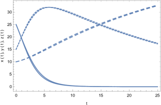
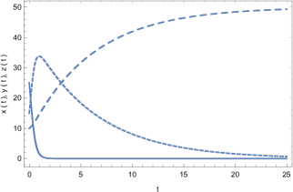
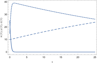
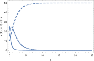
We fix the initial conditions of the SIR system as $x(0)=N_{1}=25$, $y(0)=N_{2}=15$, and $z(0)=N_{3}=10$, and we will vary the values of the parameters $\beta$ and $\gamma$. The results of the comparison between the exact numerical solution and the truncated series solutions are represented, for four distinct sets of values of $(\beta,\gamma)$, in Figs. 1 and 2, respectively.

Figure 1: Comparison of the exact numerical solution of the SIR model and of the Laplace-Adomian series expansion truncated to three terms, for $\beta=0.0147$ and $\gamma=0.0358$ (left figure), and $\beta=0.098$ and $\gamma=0.164$ (right figure). $x(t)$ is represented by the solid curve, $y(t)$ by the dotted curve, and $z(t)$ by the dashed curve. The initial conditions of the SIR system are $x(0)=25$, $y(0)=15$, and $z(0)=10$.

Figure 2: Comparison of the exact numerical solution of the SIR model and of the Laplace-Adomian series expansion truncated to three terms, for $\beta=0.119$ and $\gamma=0.017$ (left figure) and $\beta=0.0887$ and $\gamma=0.584$ (right figure). $x(t)$ is represented by the solid curve, $y(t)$ by the dotted curve, and $z(t)$ by the dashed curve. The initial conditions of the SIR system are $x(0)=25$, $y(0)=15$, and $z(0)=10$.

As one can see from the Figures, the three terms truncated Laplace-Adomian series gives a very good description of the time dynamics and evolution of the SIR epidemiological model. If necessary, the precision of the semi-analytical solution can be easily increased by adding more terms in the series expansion.

III Conclusions

Even that the exact solution of the SIR model is known, a simple but highly accurate representation of the model solution would significantly simplify the comparison of the model predictions with the epidemiological data, also allowing an efficient determination of the model parameters $\beta$ and $\gamma$ from the data fitting. The exact solution of the SIR model is given in a parametric form by $x=x_{0}u$, $y=N+\left(\gamma/\beta\right)\ln u-x_{0}u$, $z=-\left(\gamma/\beta\right)\ln u$, and $t-t_{0}=\int_{u_{0}}^{u}{d\xi/\left[\xi\left(x_{0}\beta\ln\xi-\gamma\xi-N\right)\right]}$ Harko1 , and it requires the numerical evaluation of the time integral for each step.

In the present paper we have presented a series solution of the three compartment SIR epidemiological model, giving the explicit time dependence of $x(t)$, $y(t)$ and $z(t)$. Despite its mathematical simplicity, the semianalytical solution describes very precisely the numerical behavior of the model for arbitrary values of $\beta$ and $\gamma$. The time dependence of the compartments in the semianalytical solution is given by the sum of exponential terms, and such a representation may facilitate the fitting with the statistical results. The series truncated to three terms only already give a very good description of the numerical results for arbitrary values of $\beta$ and $\gamma$, and of the initial conditions. In fact the two terms approximation also gives a good approximation of the results of the numerical integration of the SIR model.

Exact solutions of the epidemiological models are important because they can be used by epidemiologists to study the evolution of infectious diseases in different environments, and to develop the best social strategies for their control. Hopefully the results of the present paper could also contribute to the better understanding of the dynamics of the present and of the future epidemics.

References

• (1) C. Huang, Y. Wang, X. Li, L. Ren, J. Zhao, Y. Hu et al., Clinical features of patients infected with 2019 novel coronavirus in Wuhan, China, Lancet 395, 497-506 (2020).
• (2) John Graunt, Natural and political observations made upon the bills of mortality (1662).
• (3) D. Bernoulli, Essai d’une nouvelle analyse de la mortalite causee par la petite verole et des avantages de l’inoculation pour la prevenir, Mem. Math. Phys. Acad. Roy. Sci., Paris, 1 (1760).
• (4) D. Bernoulli,  Reflexions sur les avantages de l’inoculation, Mercure de France, June issue, 173 (1760).
• (5) W. O. Kermack and A. G. McKendrick, Contribution to the mathematical theory of epidemics, Proc. Roy. Soc. Lond A 115, 700-721 (1927).
• (6) F. Brauer and C. Castillo-Chávez, Mathematical Models in Population Biology and Epidemiology, Springer, New York (2001).
• (7) J. D. Murray, Mathematical Biology: I. An Introduction, Springer-Verlag, New York, Berlin, Heidelberg (2002).
• (8) D. J. Daley and J. Gani, Epidemic Modeling: An Introduction, Cambridge University Press, Cambridge (2005).
• (9) F. Brauer, P. van den Driessche, and J. Wu (Editors), Lecture Notes in Mathematical Epidemiology, Springer-Verlag, Berlin, Heidelberg (2008).
• (10) T. Harko, F. S. N. Lobo, and M. K. Mak, Exact analytical solutions of the Susceptible-Infected-Recovered (SIR) epidemic model and of the SIR model with equal death and birth rates, Applied Mathematics and Computation 236, 184-194 (2014).
• (11) A. A. Toda, Susceptible-Infected-Recovered (SIR) Dynamics of COVID-19 and Economic Impact, arXiv:2003.11221 [q-bio.PE] (2020).
• (12) J. Dehning, J. Zierenberg, F. P. Spitzner, M. Wibral, J. P. Neto, M. Wilczek, and V. Priesemann, Inferring change points in the COVID-19 spreading reveals the effectiveness of interventions, arXiv:2004.01105 [q-bio.PE] (2020).
• (13) M. Cadoni, How to reduce epidemic peaks keeping under control the time-span of the epidemic, Chaos, Solitons & Fractals 138, 109940 (2020).
• (14) J. N. Dhanwant and V. Ramanathan,Forecasting COVID 19 growth in India using Susceptible-Infected-Recovered (SIR) model, arXiv:2004.00696 [q-bio.PE] (2020).
• (15) A. L. Bertozzi, E. Franco, G. Mohler, M. B. Short, and D. Sledge, The challenges of modeling and forecasting the spread of COVID-19, arXiv:2004.04741 [q-bio.PE] (2020).
• (16) E. Franco, A feedback SIR (fSIR) model highlights advantages and limitations of infection-based social distancing, arXiv:2004.13216 [q-bio.PE] (2020).
• (17) S. Y. Lee, B. Lei, and B. K. Mallick, Estimation of COVID-19 spread curves integrating global data and borrowing information, arXiv:2005.00662v3 [stat.AP] (2020).
• (18) S. A. Hojman and F. A. Asenjo, Phenomenological dynamics of COVID-19 pandemic: meta-analysis for adjustment parameters, arXiv:2005.08686v2 [physics.soc-ph] (2020).
• (19) B. K. Beare and A. A. Toda, On the Emergence of a Power Law in the Distribution of COVID-19 Cases, arXiv:2004.12772v1 [physics.soc-ph] (2020).
• (20) D. I. Ketcheson, Optimal control of an SIR epidemic through finite-time non-pharmaceutical intervention, arXiv:2004.08848v2 [math.OC] (2020).
• (21) D.-V. Anghel and I. T. A. Anghel, Understanding the COVID19 infection curves – finding the right numbers, DOI: 10.21203/rs.3.rs-32516/v1 (2020).
• (22) J. Biazar, Solution of the epidemic model by Adomian decomposition method, Applied Mathematics and Computation 173, 1101-1106 (2006).
• (23) M. Rafei, H. Daniali and D. D. Ganji, Variational iteration method for solving the epidemic model and the prey and predator problem, Applied Mathematics and Computation 186, 1701-1709 (2007).
• (24) M. Rafei, D. D. Ganji and H. Daniali, Solution of the epidemic model by homotopy perturbation method, Applied Mathematics and Computation, 187 1056-1062 (2007).
• (25) A.-M. Batiha and B. Batiha, A new method for solving epidemic model, Australian J. of Basic and Applied Sciences 5, 3122-3126 (2011).
• (26) G. Adomian, A review of the decomposition method in applied mathematics, J. Math. Anal. Appl. 135, 501-544 (1988).
• (27) G. Adomian, Solving Frontier Problems of Physics: the Decomposition Method, Kluwer, Dordrecht, (1994).
• (28) G. Adomian and R. Rach, Modified Adomian Polynomials, Mathematical and Computer Modelling 24, 39-46 (1996).
• (29) A.-M. Wazwaz, A comparison between the variational iteration method and Adomian decomposition method, Journal of Computational and Applied Mathematics 207, 129-136 (2007).
• (30) A.-M. Wazwaz, R. Rach, and J.-S. Duan, Solving New Fourth-Order Emden-Fowler-Type Equations by the Adomian Decomposition Method, International Journal for Computational Methods in Engineering Science and Mechanics 16, 121-131 (2015).
• (31) J.-S. Duan, R. Rach, and A.-M. Wazwaz, A reliable algorithm for positive solutions of nonlinear boundary value problems by the multistage Adomian decomposition method, Open Engineering 5, id.7 (2015).
• (32) M. K. Mak, C. S. Leung, and T. Harko, Computation of the general relativistic perihelion precession and of light deflection via the Laplace-Adomian Decomposition Method, Advances in High Energy Physics 2018, 7093592 (2018).
• (33) H. O. Bakodah, A. Ebaid, and A.-M. Wazwaz, Analytical and numerical treatment of Falkner-Skan equation via a transformation and Adomian’s method, Romanian Reports in Physics 70, 111 (2018).
• (34) M. K. Mak, C. S. Leung, and T. Harko, Solving the nonlinear biharmonic equation by the Laplace-Adomian and Adomian Decomposition Methods, Surveys in Mathematics and its Applications 13, 183-213 (2018).
• (35) T. Harko, M. K. Mak, and C. S. Leung, Vortex solutions in atomic Bose-Einstein condensates via the Adomian Decomposition Method, arXiv:2003.04277v1 [cond-mat.quant-gas], accepted for publication in Romanian Reports in Physics, (2020).