On the conservation properties in multiple scale coupling and simulation for Darcy flow with hyperbolic-transport in complex flows

Abstract

We present and discuss a novel approach to deal with conservation properties for the simulation of nonlinear complex porous media flows in the presence of: 1) multiscale heterogeneity structures appearing in the elliptic-pressure-velocity and in the rock geology model, and 2) multiscale wave structures resulting from shock waves and rarefaction interactions from the nonlinear hyperbolic-transport model. For the pressure-velocity Darcy flow problem, we revisit a recent high-order and volumetric residual-based Lagrange multipliers saddle point problem to impose local mass conservation on convex polygons. We clarify and improve conservation properties on applications. For the hyperbolic-transport problem we introduce a new locally conservative Lagrangian-Eulerian finite volume method. For the purpose of this work, we recast our method within the Crandall and Majda treatment of the stability and convergence properties of conservation-form, monotone difference, in which the scheme converges to the physical weak solution satisfying the entropy condition. This multiscale coupling approach was applied to several nontrivial examples to show that we are computing qualitatively correct reference solutions. We combine these procedures for the simulation of the fundamental two-phase flow problem with high-contrast multiscale porous medium, but recalling state-of-the-art paradigms on the of notion of solution in related multiscale applications. This is a first step to deal with out-of-reach multiscale systems with traditional techniques. We provide robust numerical examples for verifying the theory and illustrating the capabilities of the approach being presented.

34E13, 34E18, 35J20, 35L67, 76M12, 76Sxx, 35Q35.

1 Introduction

In this paper, we are concerned with modeling, simulation and numerical analysis for approximate solutions in multiscale nonlinear Partial Differential Equations (PDE) related to highly complex systems. The large number of papers published in recent years is indicative of the relevance of the foundations of multiscale approach. It is a good measure of the breadth and of the vitality of the area, and therefore, calling the multiscale modeling and simulation research community for new ideas and innovative approaches. In this work we give an overview of recent approaches for the accurate and efficient simulation of complex porous media flows and we also present some new results. We summarize below the main aspects of our work:

• We revisited a novel volumetric locally conservative and residual-based Lagrange multipliers saddle point reformulation of high-order methods and present numerical results with realistic high-contrast multiscale coefficients. This is applied to a second-order elliptic problem ($\nabla\cdot\left[-K({\bf x})\Lambda(S)\nabla p\right]=q(\textbf{x})$ ) instead of a traditional first-order mixed formulations. We clarifying and simplifying the presentation of its conservative properties.

• We introduce a new robust and accurate forward tracking Lagrangian-Eulerian scheme for hyperbolic problems. Our method is carefully designed to deal with multiscale wave structures resulting from shock wave interactions coming from abstract nonlinear hyperbolic conservation laws such as $w_{t}+\mbox{div}\mathcal{F}(t,{\bf x},w(t,{\bf x}))=0$ with fluxes of the form $\mathcal{F}(x,t,w)={\bf v}(x,t)f(w(t,{\bf x}))$. This formulation includes many problems of physical interest and, in particular, we consider the case of complex multiscale flow in porous media (scalar and systems cases).

• We improve the interpretation of the construction of numerically stable Lagrangian-Eulerian no flow surface region in two-space dimensions previously presented and analyzed in [17] for one-dimensional balance and conservation laws.

• We present a new approach with accurate multiscale resolution for two-phase flows. The method is able to handle multiscale rock geology in the elliptic-pressure-velocity system. Moreover, the multiscale wave structures from wave interactions present in the hyperbolic-transport model seems to be properly simulated according to our numerical results.

• We present numerical results with realistic high-contrast two-dimensional multiscale coefficients based on the 10th SPE Comparative Solution Project (SPE10). We address numerical issues of multiscale resolution and conservation properties.

• We survey recent results on both: novel deterministic and probabilitc multiscale modeling paradigms and issues of mesh resolution inadequacy in multiscale complex systems.

The new elliptic solver [14, 15] is a general tool for imposing local conservation for high-order methods to deal with multiscale permeabilities. In particular is also applicable to the Generalized Multiscale Finite Element Method (GMsFEM); see [16, 74, 119, 75, 118] and references therein. On the other hand, the new Lagrangian-Eulerian method seems to be a promissing general approach to capture nonlinear wave interactions linked to multiscale behavior of interactions of waves in a wide range of models and, in particular, for systems (see [17, 18, 19, 20, 21, 22]). Numerical results show that our combined multiscale approach provides an accurate and robust procedure to study phenomena which couple distinct length or time scales. Our novel hyperbolic Lagrangian-Eulerian solver circumvents the use of adaptive and/or mesh generation. Indeed, the new method is also free of Riemann solvers. For Darcy flow, the method captures fine-scale effects using multiscale finite element techniques. Finally, it is worth mentioning that for the purpose of this work we use Cartesian grids. Thus convergence and error analysis reduces essentially to a one-dimensional problem and retains convergence result of approximated solutions to the entropy weak solution by recalling [64, 65, 48, 57]. This is to say that our approach fits comfortably within the classical theory. On the other hand, we provide convergence and error analysis on triangular grids for hyperbolic conservation laws in another forthcoming work [22]. Moreover, the results in [17], strongly suggest that the no flow surface region encapsulates the domain of dependence even in the case of hyperbolic systems.

A reliable multiscale prediction of oil-water two-phase flow model through complex porous media requires the development and validation of coupling models for flow across length scales related to elliptic Darcy-pressure-velocity and hyperbolic saturation-conservation problems. Therefore, in this work we introduce a novel computational approach for multiscale computing of the oil-water flow model system.

Let $\Omega$ be a domain in $\mathbf{R^{2}}$. For simplicity of presentation, we consider two-phase flow in a viscous-dominated flow, and we neglect the effects of gravity, compressibility and capillarity and set the porosity equal to a constant, in which case it has been scaled out by a change of the time variable. Thus, the fundamental differential multiscale system used to describe water-oil, incompressible, immmiscible displacement is given by the saturation and pressure equations (see, e.g., [52]):

(1) $$\frac{\partial S}{\partial t}+\nabla\cdot({\bf v}\,\mathcal{F}(S))=0,\quad\mbox{in }{\bf x}\in\Omega,\qquad 0<t\leq T,$$

(2) $$\nabla\cdot{\bf v}=\nabla\cdot\left[-K({\bf x})\Lambda(S)\nabla p\right]=q(\textbf{x}),\quad\mbox{in }{\bf x}\in\Omega,\qquad 0<t\leq T.$$

Here, $S$ is the water saturation (water and oil saturation sum up to one), ${\bf x}$ is the absolute permeability, ${\bf v}$ is the total Darcy velocity, $p$ is the pressure, $\Lambda$ is the total mobility and $\mathcal{F}$ is the fractional flow of water. We also have $\mathcal{F}=\Lambda_{i}/\Lambda$ with $\Lambda_{i}=k_{i}/\mu_{i}$ being the phase mobility, $k_{i}$ the relative permeability and $\mu_{i}$ viscosity of phase $i$, respectively.

We end up with a multiscale system of two coupled nonlinear partial differential equations (1)-(2) exhibiting multiscale features in both sides: the complex multiscale heterogeneity structures from rock geology appearing in the elliptic-pressure-velocity model (2) as well as multiscale wave structures resulting from shock wave interactions from the hyperbolic-transport model (1). For concreteness, we complete equations (1) and (2) with appropriate initial and boundary conditions aiming simulations in a slab geometry domain $\Omega$ and time interval $T=\left[t_{0},t_{f}\right]$. We consider the coupling system (1)-(2) in a two-dimensional rectangular slab domain $\Omega=(0,L_{x})\times(0,L_{y})$, with the boundary conditions

(3) $$\begin{array}[]{ll}{\bf v}\cdot{\bf n}=-q,&\text{on }x=0,\\ p=0,&\text{on }x=L_{x},\\ {\bf v}\cdot{\bf n}=0,&\text{on }y=0,L_{y},\end{array}$$

where ${\bf n}$ is the outward-pointing unit normal vector to $\partial\Omega$, and a uniform initial condition

(4) $$S(x,0)=S_{0}.$$

The initial-boundary conditions (3)-(4) simulate a left to-right waterflood. Water is injected uniformly (at a constant rate $q$) through the left vertical boundary $\Gamma_{inlet}$ ($x=0$) of $\Omega$ for all simulation time $t\in\left[t^{0},t_{f}\right]$, no flow conditions are imposed along the horizontal boundaries $\Gamma_{no-flux}$ ($y=0,L_{y}$), and fluid is produced from a well kept at constant (zero) pressure at the right vertical boundary $\Gamma_{outlet}$ ($x=L_{x}$).

Equations (1)-(4) can be viewed as multiscale water-oil Riemann-Goursat water injection problem with discontinuous flux function as closely related to [5] (see [109, 104, 103, 102, 101]), in which the hyperbolic scheme should be able to handle the main difficulty of the multiscale problem that consists in taking into account the jump discontinuities of the flux; see also [64, 65, 12, 8, 6, 7] and references cited therein. Another motivation is the occurrence of models such as (1)-(4) in numerous engineering problems, mainly the case of systems [8, 6, 7, 69, 70, 33, 34, 35, 95, 12]. In addition, there are a number of prototype relevant models of hyperbolic conservation laws with discontinuous flux functions in oil trapping phenomenon [29, 9, 44, 87, 97, 115], a Whitham model of car traffic flow on a highway [81, 93] and a model of continuous sedimentation in ideal clarifier-thickener units [40], see also [38, 88]. Hyperbolic conservation laws with discontinuous flux functions also arise in sedimentation processes [59], in radar shape-from-shading problems [100] and also as building blocks in numerical methods for Hamilton-Jacobi equations [89]. Hyperbolic conservation laws of the form (1) with discontinuous (in $(t,{\bf x})$) flux function $\mathcal{H}({t,{\bf x},S})\equiv\{f(S)\left[-K({\bf x})\Lambda(S)\nabla p\right]\}$ attracted much attention in the recent past, because of the difficulties of adaptation of the classical Kruzhkov approach developed for the smooth case, due in part to the presence of several different entropy solutions with same initial data. In the context of Buckley-Leverett equations as in (2)-(4), each notion of solution is uniquely determined by the choice of a connection, which is made unique at the interface by a proper choice of an entropy solution from many possible classes of entropy solutions, [24, 29, 5]. Nonclassical solutions appear for Buckley-Leverett models with gravity and discontinuous flux functions [44, 29] as well as for three-phase flow problems with continuous flux functions, where recent and very relevant results can be found in [33, 34, 35, 95] for a solution of Riemann problems and in [69, 70] concerning well-posedness. In [27], a theory of $L^{1}$-dissipative solvers for scalar conservation laws with discontinuous flux was proposed, which is based on the corresponding $L^{1}$ contractive semigroups, some of which reflect different multiscale physical applications. In [27, 28, 58] a number of the existing admissibility (or entropy) conditions are revisited and the so-called germs that underly these conditions are identified. The seminal survey article [28] (see also [107, 108, 113, 41, 111, 90, 47, 88]) of recent developments helps to better understand the issue of admissibility of solutions in relation with specific modeling assumptions.

By looking at model problem (1)-(4) as a generalized problem linked to systems of conservation laws in several dimensions, we recall that some authors has advocated entropy measure-valued solutions, first proposed by DiPerna [60, 61], as the appropriate solution paradigm for systems of conservation laws; see [67, 68] and references cited therein. In particular, these authors have presented some numerical evidence that state-of-the-art numerical schemes may not converge to an entropy solution of systems of conservation laws as the mesh is refined. Accordingly to [67, 68] this has been attributed to the emergence of turbulence-like structures at smaller and smaller scales upon mesh refinement. See also [50, 51, 94].

In [68], the authors point out that intermittency is widely accepted to be a characteristic of turbulent flows [72]. It is believed that intermittency stems from the fact that turbulent solutions do not scale exactly as in the Kolmogorov hypothesis. On the other hand, in [50] the authors offer a unified framework in which is possible to establish mathematical existence theories as well as a very innovative idea for the interpretation of numerical solutions through the identification of a function space in which convergence should take place. In a more general setting, the issue of multiscale modeling and simulation of chaotic mixing of distinct fluids has been addressed in [50, 51, 94]. They mention that acceleration driven turbulent mixing is a classical hydrodynamic instability. See also [73] to the case of two-phase flows.

We also mention also the very recent works [50, 51, 94, 67, 68] on nonlinear multiscale problems like (1)-(4) in which resolution of multiscale turbulent-like behavior is better resolved under mesh refinement. In fact, structures at smaller and smaller scales are formed as the mesh is refined to account for the complex heterogeneity structures from rock geology appearing in the elliptic model as well as multiscale wave structures resulting from shock wave interactions from the underlying hyperbolic problem. This is done such that solutions satisfy a proper family of entropy inequalities [5]. Results in [92, 54] have demonstrated that entropy solutions may not be unique. In the direction from both rigorous mathematical analysis and numerical analysis, ingenious difficulties stem from the lack of regularity of solutions.

A better comprehension of multiscale fluid flow in subsurface is very hard, challenging and undoubtedly still of current events. Multiscale sciences cuts across all of science from fluid dynamics to biology, from meteorology to material science and from physics to chemistry among many other directions. Multiscale issues are also central in subsurface flows ranging from complex geologic media to several time scales linked to the compositional and black-oil modeling fluid flow in oil reservoirs as well as several scale aspects of groundwater flow and related transport systems. Understanding the multiscale properties of subsurface flows is a major problem of modern approaches predicting groundwater level changes and predictive technologies in petroleum reservoir. In this regard, many innovative techniques have been reported as such local-global upscaling approach [63, 78, 96, 53, 117, 62], multiscale methods [1, 32, 82, 84, 91, 98, 99, 79, 30], model order reduction techniques [71, 83, 45, 110, 55], Two-scale homogenization theory [66, 25, 26, 42, 86, 112, 31]; see papers for a survey on recent development of multiscale computing and modeling approach [110, 2, 114, 76, 77, 116, 80].

Despite the efforts of many researchers, no universal or unified multiscale modeling and methods for fluid flow through naturally complex geologic reservoirs has been achieved so far (see, e.g., [2, 116, 46, 105, 8, 110, 83, 71, 98, 32, 62, 117, 63]). Under appropriate simplification assumptions compositional and black-oil models can be further simplified for the fundamental multiscale two-phase immiscible displacement with no mass transfer between phases (this is often appropriate in models describing displacements at the length scales associated with reservoir simulation grid blocks, see, e.g., [63]). In addition, even for the two-phase case, the multiscale modeling is very challenging in the presence fractures and barriers for flow in porous medium and their impact on the closure and constitutive relations as such multiscale relative permabilities and pressure difference (capillary pressure); see [29] and references cited therein for an interesting study on vanishing capillarity solutions of Buckley-Leverett equation with gravity in two-rock’s medium (see also [105, 46, 43] for multiscale modeling of Richards’s equation and two-phase under non-equilibrium effects). However, in the case of scalar water-oil two-phase model a global-pressure formulation and Kirchhoff’s transform are not adequate when considering non-equilibrium effects as such hysteresis in the relative permeabilities [12] and in the capillary pressure [36] the issue of global pressure formulation for three-phase is not straightforward (see [8, 12, 13] and reference cited therein for a detailed multiscale modeling for three-phase flow problem). Moreover, the case of discontinuous capillary pressure induced by mulsitcale modeling of fractures and barriers in the three-phase flow with gravity is hard and very intricate [8, 11, 13]. The degeneracy for three-phase and two-phase flows is also delicate [10, 106]. Altogether the fundamental multiscale water-oil model (1)-(4) is also useful both for describing some real cases (e.g., dead-oil systems) and for developing and studying numerical solution procedures. In this works we consider the multiscale approximation associated with reservoir multiscale simulation along with coupling techniques for elliptic (Darcy-pressure-velocity) and hyperbolic (conservation-saturation-transport) problems as pursued in this work.

The paper is organized as follows. In Section 2, we construct an embedded high-order model for second-orde elliptic problems with local and global mass conservation, clarifying and simplifying the presentation of its conservative properties in lines as introduced in [14, 14, 75, 3, 16]. Next, we construct new a locally conservative Lagrangian-Eulerian method for hyperbolic-transport with focus on a novel approach for conservation properties of the no flow surface region for hyperbolic conservation laws in Section 3. In Section 4, we present and discuss a the oupling conservative finite element method for Darcy flow problem with a locally conservative Lagrangian-Eulerian method for hyperbolic-transport, along with a set of representative computational results. In Section 5, a summary with concluding remarks and perspectives for future work are highlitghted.

2 Elliptic problem and mass conservation

Many porous media related practical problems (scalar and systems) lead to the numerical approximation of the Buckley-Leverett type-models given by the highly-nonlinear multiscale problem like (1)-(4). For the approximation of the pressure field given by the pressure-velocity Darcy-elliptic fundamental multiscale problem (2). We use the method designed and analyzed in [14, 75]; see also [3, 16, 74]. We now recall this high-order conservative FEM formulation, clarifying and simplifying the presentation of its conservative properties with focus on the conservation properties in multiple scale coupling and simulation for Darcy flow with hyperbolic-transport in complex flows. A general interpretation of this methodology goes as follows: given a Ritz approximation of the pressure and a computational procedure to obtain fluxes we can then, formulate an constrained (to local flux conservation) minimization problem to obtain approximated solution that satisfy local conservation properties in the form of average fluxes on local regions. See [75, 3, 16].

2.1 Imposing local mass conservation

We follow the presentation in [14, 75]. Denote $H^{1}_{D}(\Omega)$ the space of functions in $H^{1}(\Omega)$ which vanish on $\partial\Omega_{D}$. The variational formulation of problem (2) is to find $p\in H^{1}_{D}(\Omega)$ such that

(5) $$a(p,v)=F(v)\quad\mbox{ for all }v\in H_{D}^{1}(\Omega),$$

where $v\in H^{1}_{D}(\Omega)$ and the bilinear form $a$ is defined by

(6) $$\vspace{-1.5mm}a(p,v)=\int_{\Omega}\Lambda(x)\nabla p(x)\nabla v(x)dx,$$

and the functional $F$ is defined by ${F(v)=\int_{\Omega}q({\bf x})v(x)dx.}$

Problem (2) is equivalent to the minimization problem: Find $p\in H^{1}_{D}(\Omega)$ such that

(7) $$\vspace{-1.5mm}p=\arg\min_{v\in H^{1}_{D}(\Omega)}\mathcal{J}(v),\quad\mbox{ where }\quad\mathcal{J}(v)=\frac{1}{2}a(v,v)-F(v).$$

In the IMPES approach, for each time step the mobility can be thought as a function of position and reads simply as $\Lambda(x)$. Thus, in order to consider a general formulation for porous media applications we let $\Lambda$ be a $2\times 2$ matrix with entries in $L^{\infty}(\Omega)$ in Problem (2) to be almost everywhere symmetric positive definite matrix with eigenvalues bounded uniformly from below by a positive constant.

In order to deal with mass conservation properties we follow the method introduced in [75, 3]. Let $\mathcal{T}_{h}=\{R_{j}\}_{j=1}^{N_{h}}$ be a primal mesh made of elements that are triangles or squares. Here $N_{h}$ is the number of elements of the triangulation. We also have a dual mesh $\mathcal{T}_{h}^{*}=\{V_{i}\}_{i=1}^{N_{h}^{*}}$ where the elements are called control volumes and $N_{h}^{*}$ is the number of such volumes. In general it is selected one control volume $V_{i}$ per vertex of the primal not in $\partial\Omega_{D}$. In case $|\partial\Omega_{D}|=0$, $N_{h}^{*}$ is the total number of vertices of the primal triangulation including the vertices on $\partial\Omega$. Figure 1 illustrate primal and dual meshes made of squares where $\partial\Omega_{D}=\partial\Omega$, in this case $N^{*}_{h}$ is equal to the number of interior vertices of the primal triangulation.

If $q\in L^{2}$ we have that solving (2) is equivalent to: Find $p\in H_{\mbox{\small div},\Lambda}^{1}(\Omega)$ and such that

(8) $$p=\arg\min_{v\in\mathcal{W}}\mathcal{J}(v),$$

where the subset of functions that satisfies the mass conservation restrictions is defined by

$$\mathcal{W}=\left\{v\in H_{0}^{1}(\Omega),:\int_{\partial T}-\Lambda\nabla v\cdot\mathbf{n}=\int_{T}q\quad\text{ for all }T\in\mathcal{T}^{*}_{h}\right\}.$$

and

$$H_{\mbox{\small div},\Lambda}^{1}(\Omega)=\{v\in H_{D}^{1}(\Omega):\Lambda\nabla v\in H(\mbox{div},\Omega)\}$$

with norm $\|v\|^{2}_{H_{\mbox{\small div},\Lambda}^{1}(\Omega)}=\|\Lambda\nabla v\cdot\nabla v\|^{2}_{L^{2}(\Omega)}+\|\mbox{div}(\Lambda\nabla v)\|^{2}_{L^{2}(\Omega)}$.

Let $M^{h}=\mathbb{Q}^{0}(\mathcal{T}^{*}_{h})$ be the space of piecewise constant functions on the dual mesh $\mathcal{T}_{h}^{*}$. The Lagrange multiplier formulation of problem (8) can be written as: Find $p\in H_{\mbox{\small div},\Lambda}^{1}(\Omega)$ and $\lambda\in M^{h}$ that solves,

(9) $$\arg\max_{\mu\in\color[rgb]{0,0,0}M^{h}}\min_{v\in\color[rgb]{0,0,1}H_{\mbox{\small div},\Lambda}^{1}(\Omega)}\mathcal{J}(v)-(\overline{a}(p,\mu)-G(\mu)).$$

Here, the total flux bilinear form $\overline{a}:H_{\mbox{\small div},\Lambda}^{1}(\Omega),\times{\color[rgb]{0,0,0}M^{h}}\to\mathbb{R}$ is defined by

(10) $$\overline{a}(v,\mu)=\sum_{i=1}^{\color[rgb]{0,0,0}N_{h}^{*}}\mu_{i}\int_{\partial V_{i}}\Lambda\nabla v\cdot\mathbf{n}\quad\mbox{ for all }v\in H_{\mbox{\small div},\Lambda}^{1}(\Omega),\mbox{ and }\mu\in M^{h}.$$

The functional $G:{\color[rgb]{0,0,0}M^{h}}\to\mathbb{R}$ is defined by

$$G(\mu)=\sum_{i=1}^{\color[rgb]{0,0,0}N_{h}^{*}}\mu_{i}\int_{V_{i}}q\quad\mbox{ for all }\mu\in M^{h}.$$

The first order conditions of the min-max problem above give the following saddle point problem: Find $p$ with $p\in H_{\mbox{\small div},\Lambda}^{1}(\Omega),$ and $\lambda\in M^{h}$ that solves,

(11) $$\begin{array}[]{llr}a(p,v)+\overline{a}(v,\lambda)&=F(v)&\mbox{ for all }v\in H_{\mbox{\small div},\Lambda}^{1}(\Omega),,\\ \overline{a}(p,\mu)&=G(\mu)&\mbox{ for all }\mu\in M^{h}.\\ \end{array}$$

For the analysis of this formulation see [14]. Recall that we have introduced a primal mesh $\mathcal{T}_{h}=\{R_{j}\}_{j=1}^{N_{h}}$ made of elements that are triangles or squares. Here $N_{n}$ is the number of elements of the triangulation. We also have given a dual mesh $\mathcal{T}_{h}^{*}=\{V_{k}\}_{k=1}^{N_{h}}$ where the elements are called control volumes. Figure 1 illustrate a primal and dual mesh made of squares. See for instance [37, 75, 3].

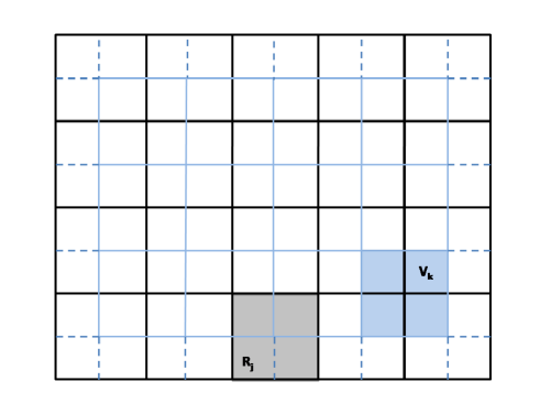
Figure 1: Example of regular mesh made of squares and its dual triangulation.

Let us consider $P^{h}=\mathbb{Q}^{r}(\tau_{h})$ the space of continuous polynomial functions of degree $r$ on each element of the primal mesh, and let $P^{h}_{0}$ be the space the functions in $P^{h}$ that vanish in $\partial\Omega$. Let $M^{h}=\mathbb{Q}^{0}(\tau^{*}_{h})$ be the space of piece constant functions on the dual mesh $\tau_{h}^{*}$. For more details on the constructions see [14, 75]. The discrete version of (11) is to find $p^{h}\in{\color[rgb]{0,0,0}P^{h}_{0}}$ and $\lambda\in M^{h}$ such that

(12) $$a(p^{h},v^{h})+\overline{a}(v^{h},\lambda^{h})=F(v^{h}) \mbox{ for all }v^{h}\in{\color[rgb]{0,0,0}P^{h}_{0}}$$

(13) $$\overline{a}(p^{h},\mu^{h})=G(\mu^{h}) \mbox{ for all }\mu^{h}\in M^{h}.$$

Let $\left\{\varphi_{i}\right\}$ be the standard basis of $P^{h}$. We define the matrix

(14) $$A=\left[a_{i,j}\right]\quad\mbox{ where }a_{ij}=\int_{\Omega}\Lambda\nabla\varphi_{i}\cdot\nabla\varphi_{j}.$$

Note that $A$ is the finite element stiffness matrix corresponding to finite element space $P^{h}$. Introduce also the matrix

(15) $$B=\left[\overline{a}_{k,j}\right]\quad\mbox{ where }\overline{a}_{ij}=\int_{\partial V_{k}}\Lambda\nabla\varphi_{j}\cdot\textbf{n}.$$

With this notation, the matrix form of the discrete saddle point problem is given by,

(16) $$\mathcal{A}U^{h}=\left[\begin{array}[]{cc}A&B^{T}\\ B&O\end{array}\right]\left[\begin{array}[]{c}u^{h}\\ \lambda^{h}\end{array}\right]=\left[\begin{array}[]{c}f\\ g\end{array}\right]$$

where vectors $f$ and $g$ are defined by,

(17) $$f=\left[f_{i}\right]\quad\mbox{ with}\,f_{i}=\int_{\Omega}q\cdot\varphi_{i} g=[g_{i}]_{i=1}^{M_{f}}=\int_{V_{k}}q.$$

For the analysis of the continuous and discrete problem and corresponding error estimates see [14]. As an important remark we mention the optimality of the approximation error in both $H^{1}$ and $L^{2}$ norms. From the analysis in [3, 16] we know that $u^{h}$ is an optimal approximation in the $H^{1}$ semi-norm (which becomes a norm when restricted to appropriate subspace). We also found in [3] that, in each control volume, the $u^{h}+\lambda^{h}$ offers optimal approximation in the $L^{2}$ norm. We real that in many approaches imposing conservation properties of second order formulations leads to a non-optimal $L^{2}$ approximation. For more details on this formulation in porous media applications; see [2, 75, 3, 14, 15].

2.2 Numerical tests

Let us illustrate the two main features of the HOCFEM method which are high-order approximation rate and conservation of mass.

2.2.1 Homogeneous medium

We consider the Equation (2) with $\Omega=\left[0,1\right]\times\left[0,1\right]$ in homogeneous medium ($\Lambda(x)\equiv 1$), to be discretized on a regular mesh made of $2^{M}\times 2^{M}$ squares. The dual mesh is constructed by joining the centers of the elements of the primal mesh as in Figure 1. We consider homogeneous Dirichlet’s boundary conditions in $\partial\Omega$ and construct the example (18) by fixing the solution $p$ and computing a source term $q$ so we can compare the numerical solution with the exact solution

(18) $$q(x,y) =2\pi(\cos(\pi x)\sin(\pi y)-3\sin(\pi x)\cos(\pi y)+\pi\sin(\pi x)\sin(\pi y)(-x+3y)),$$

$$p(x,y) =\sin(\pi x)\sin(\pi y)(-x+3y).$$

We apply HOCFEM to example (18) with $\mathbb{Q}_{1},\cdots,\mathbb{Q}_{5}$ finite element spaces to the problem and compute HOCFEM and FEM solutions. We estimate the $L^{2}$ and $H^{1}$ errors and plot them in a log-log graphic shown in Figures 2 and 3.

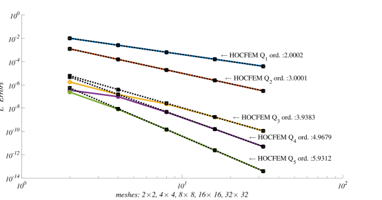
Figure 2: Log-log graphic of errors in $L^{2}$ norm for HOCFEM numerical solutions of Problem (2) with data (18), using $\mathbb{Q}_{1}$, $\mathbb{Q}_{2}$, $\mathbb{Q}_{3}$, $\mathbb{Q}_{4}$ and $\mathbb{Q}_{5}$ basis through a mesh refinement.

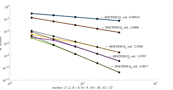
Figure 3: Log-log graphic of errors in $H^{1}$ norm for HOCFEM numerical solutions of Problem (2) with data (18), using $\mathbb{Q}_{1}$, $\mathbb{Q}_{2}$, $\mathbb{Q}_{3}$, $\mathbb{Q}_{4}$ and $\mathbb{Q}_{5}$ basis through a mesh refinement.

Numerical convergence is observed in $H^{1}$ norm with the same error variation rate of FEM. The error $p-p^{h}$ in $L^{2}$ norm is not optimal but with the correction $p-(p^{h}+\lambda^{h})$ (in each control volume) we recover convergence rate of FEM in this norm for HOCFEM. We compute conservation of energy indicator (19) and conservation of mass indicator (20) by the below formulas, respectively,

(19) $$E(p)=\frac{1}{2}\int_{\Omega}\Lambda|\nabla p|^{2}-\int_{\Omega}qp,$$

(20) $$J(p)=\left(\sum_{R}\left(\int_{\partial R}\Lambda\nabla p\eta-\int_{R}q\right)^{2}\right)^{1/2}.$$

$Q_{r}$	$E(u_{FEM})$	$E(u_{HOCFEM})$	$J(u_{FEM})$	$J(u_{HOCFEM})$
$1$	$-4.514912976$	$-4.514911724$	$3.304137047\times 10^{-4}$	$5.893618438\times 10^{-15}$
$2$	$-4.523567134$	$-4.523565879$	$3.308277779\times 10^{-4}$	$6.553391232\times 10^{-15}$
$3$	$-4.523568684$	$-4.523568684$	$2.295180099\times 10^{-8}$	$1.902320206\times 10^{-14}$
$4$	$-4.523568684$	$-4.523568684$	$2.295194635\times 10^{-8}$	$1.805166187\times 10^{-14}$
$5$	$-4.523568684$	$-4.523568684$	$1.454599166\times 10^{-12}$	$3.207818336\times 10^{-14}$
$6$	$-4.523568684$	$-4.523568684$	$3.489145981\times 10^{-12}$	$3.408881693\times 10^{-14}$

Table 1: Energy minimization and conservation indicator with $h=2^{-9}$ for numerical solution of Problem (2) with data (2).

As we can see in Table 1 conservation of Energy remains similar for both methods while HOCFEM exhibit much better conservation of mass than classical FEM.

2.2.2 Heterogeneous medium

Let us move to a heterogeneous medium with high-contrast coefficients. The medium to be consider is the last $64\times 64$ block of the geological $SPE10$ porous medium taken from [56] shown in Figure 4. This is a widely used heterogeneous porous medium for simulations (see for example [56]).

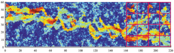
Figure 4: A 2D layer of the $SPE10$ 2D porous medium sample from [56].

We perform a numerical experiment to study convergence and conservation of energy and mass of HOCFEM in such a realistic heterogeneous medium. Let us consider the model problem (2) on $\Omega=\left[0,1\right]\times\left[0,1\right]$ with constant forcing term and homogeneous Dirichlet’s boundary conditions over $\partial\Omega$. The mobility coefficient $\Lambda$ is taken from the SPE10 medium as described before. We compute HOCFEM approximations using $\mathbb{Q}_{1}$ and $\mathbb{Q}_{2}$ basis over $3$ square meshes of norm $h=2^{-M}$ with $M=6,7,8$ and compute errors in $L^{2}$ and $H^{1}$ norms against a reference solution calculated using $\mathbb{Q}_{3}$ basis in the finest mesh. Figures 5 and 6 show the $L^{2}$ and $H^{1}$ errors computed for both solutions using $\mathbb{Q}_{1}$ and $\mathbb{Q}_{2}$. We observe that the error variation rate is similar for both solutions. This behavior of the error in heterogeneous medium is different to homogeneous medium where rates where proportional to the grade of the polynomials used in basis.

We also compute the approximated solution $u^{h}_{HOCFEM}$ solving system in (16) for a $256\times 256$ computational mesh and estimate the conservation of energy and mass indicators defined in (19) and (20). Table 2 shows both, local mass and energy conservation indicators, for our high order HOCFEM formulation ($E(u_{HOCFEM})$ and $J(u_{HOCFEM})$) and for classical FEM ($E(u_{FEM})$ and $J(u_{FEM})$).

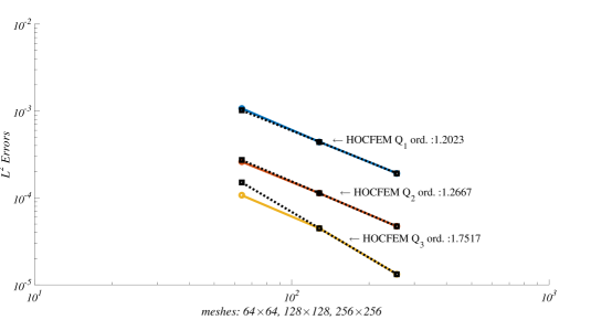
Figure 5: Log-log graphic of errors in $L^{2}$ norm for HOCFEM numerical solutions of Problem (2) in SPE10 medium, using $\mathbb{Q}_{1}$ and $\mathbb{Q}_{2}$ basis through a mesh refinement. The norm of the mesh $h=2^{-M}$ vary as $M=6,7,8$.

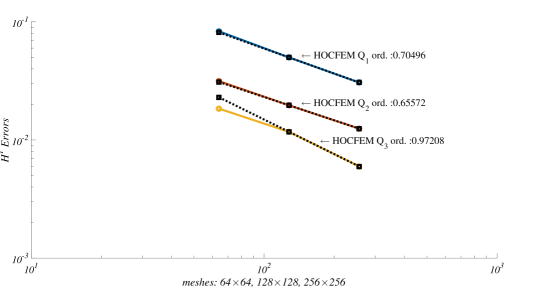
Figure 6: Log-log graphic of errors in $H^{1}$ norm for HOCFEM numerical solutions of Problem (2) in SPE10 medium with data ([56]), using $\mathbb{Q}_{1}$ and $\mathbb{Q}_{2}$ basis through a mesh refinement. The norm of the mesh $h=2^{-M}$ vary as $M=6,7,8$.

$Q_{r}$	$E(u_{FEM})$	$E(u_{HOCFEM})$	$J(u_{FEM})$	$J(u_{HOCFEM})$
$1$	$-2.610659111$	$-2.606353663$	$6.478664199\times 10^{-1}$	$2.734482311\times 10^{-12}$
$2$	$-2.755620550$	$-2.752274173$	$5.472598738\times 10^{-1}$	$2.816845987\times 10^{-12}$
$3$	$-2.778407981$	$-2.778404839$	$4.095003567\times 10^{-2}$	$9.330127650\times 10^{-12}$
$4$	$-2.786675138$	$-2.786672433$	$3.959310237\times 10^{-2}$	$7.837454755\times 10^{-12}$
$5$	$-2.790778373$	$-2.790778322$	$8.962957140\times 10^{-3}$	$1.509701588\times 10^{-11}$
$6$	$-2.793138428$	$-2.793138381$	$8.972699240\times 10^{-3}$	$1.289345855\times 10^{-11}$

Table 2: Energy minimization and conservation indicator for numerical solution of Problem (2) with data (18) in a fixed mesh $64\times 64$ using basis $\mathbb{Q}_{1}$, $\mathbb{Q}_{2}$, $\mathbb{Q}_{3}$, $\mathbb{Q}_{4}$, $\mathbb{Q}_{5}$ and $\mathbb{Q}_{6}$.

From Table 2 we see that conservation of global energy does not change from FEM to HOCFEM while conservation of mass is superior in large with our new formulation.

3 Conservation properties of the no flow surface region for hyperbolic conservation laws

The aim of this section is to present an extension of the Lagragian-Eulerian scheme (see [17, 18, 19, 20, 21, 22]) for hyperbolic conservation laws in two-space dimensions with some initial condition coming from abstract nonlinear problems of hyperbolic conservation laws. We can also consider problems of physical interest in fluid mechanics such as multiscale flow in porous media scalar and systems treated in this work.

We mention that our novel hyperbolic Lagrangian-Eulerian solver (it its simplest form) can be viewed as a monotone scheme (see Section 3.4). For coupling Darcy flow, the transport method captures fine-scale effects using a (conservative) fine-grid finite element technique combined with Lagragian-Eulerian scheme. For the purpose of this work we use Cartesian grids since for the case of monotone scheme convergence and error analysis reduces (essentially) to a one-dimensional problem and it retains convergence results and approximation to the entropy weak solution by recalling [64, 65, 48, 57].

We improve the interpretation of the construction of numerically stable Lagrangian-Eulerian no flow surface region in two-space dimensions previously presented and analyzed in [17] for one-dimensional balance and conservation laws. It turn out that our monotone Lagrangian-Eulerian is a building block for construction of a novel class of Lagrangian-Eulerian shock-capturing schemes for first-order hyperbolic problems. The early monotone versions of the Lagrangian-Eulerian approach has been employed successfully in a number of very non-trivial problems and also developed theoretically [17, 20, 18, 19, 21, 22] linked to several transport models such as the Burgers’ equation with Greenberg-LeRoux’s and Riccati’s source terms, the shallow-water system, Broadwell’s rarefied gas dynamics, Baer-Nunziato’s system linear, non-linear convex and non-linear non-convex 2D scalar conservation laws (see [18, 17]). It is worth mentioning that the Lagrangian-Eulerian framework is able to compute qualitatively correct (entropy) solutions involving intricate non-linear wave interactions of rarefaction and shock waves. It is of significance to mention that the scheme is able to handle resonance effect associated to non classical transitional shock in a $2\times 2$ three-phase flow water-oil-gas system [18, 19] and an intricate shock structure linked to a $5\times 5$ isentropic Baer-Nunziato model (see [17]). The Lagrangian-Eulerian scheme does handle properly the sonic rarefaction linked to Burgers’ equation, namely, a typical small (and unphysical) discontinuity jump within the rarefaction structure; such discontinuation in the solution is unphysical, and thus with no mathematical relation with an entropy violating shock. Indded, our Lagrangian-Eulerian scheme does not produce the well-known spurious entropy glitch effect in the sonic rarefaction (as is the case of Rusanov and Godunov monotone schemes). In addition, our first-order monotone Lagrangian-Eulerian scheme is less difusive than the classical Lax-Friedrichs scheme, but retains robustness and it is simple to implement and efficient for numerical computing [4].

A key hallmark of the our Lagrangian-Eulerian (monotone) method is the dynamic tracking forward of the no-flow region (per time step). This is a considerable improvement compared to the classical backward tracking over time of the characteristic curves over each time step interval, which is based on the strong form of the problem. Indeed, in the case of systems and multi-D problems, we can say that backward tracking is not understood.

Our new method can handle, with great simplicity, nontrivial scalar and systems problems in 1D and multi-D [17, 18]. Another key hallmark of the our Lagrangian-Eulerian (monotone) method is the a flux separation strategy and its impact on the balancing (multiple scale) discretization between the first-order approximation of the hyperbolic flux and the source term to take into account nonlinear wave interactions preserving conservation properties. For instance, in [17] the numerical tests show that the discretizations resulting from the flux separation strategy when applied to the 2 by 2 shallow-water system and 5 by Baer-Nunziato’s system seem to be of good quality. Moreover, such strategy seem to be very appropriate to deal with convex and nonlinear non-convex 2D scalar conservation laws.

With respect to the theory of monotone scheme, the no flow region (see Figure 8) is the control volume where the (local) wave interaction (always in the fine mesh of any multiscale method approach) takes place. On the other hand, in light of modern reasearch (see [54, 39] and [17]), the no flow region is a space-time cutoff to account the complex and intricate nonlinear wave group interaction within control volume per time step in the overall simulation ([13, 33, 95, 17, 18]). In computing practice, the no flow region parallel with the CFL stability criterion associated with the space-time discretization of many numerical methods.

Therefore, the monotone Lagrangian-Eulerian approach is a interesting novel framework for hyperbolic conservation laws and multiscale transport flow models.

3.1 Lagragian-Eulerian technique with conservation properties

We discus our new Lagragian-Eulerian technique with conservation properties for the approximation of the 2D initial value problem for hyperbolic of conservation laws,

(21) $$\begin{cases}\displaystyle\frac{\partial u}{\partial t}+\frac{\partial f(u)}{\partial x}+\frac{\partial g(u)}{\partial y}=0,\qquad(x,y,t)\in\Omega\times(t^{0},T],\\ u(x,y,t^{0})=\eta(x,y),\quad(x,y)\in\Omega,\end{cases}$$

where $\Omega$ is a interior square domain in $\mathds{R}^{2}$, whit boundary $\partial\Omega$ and $T=t_{f}>0$.

For the finite dimensional function spaces we introduce the following standard notation. The space region $\left(\mathds{R}\times\mathds{R}\right)\times\overline{\mathds{R}}=\{(x,y,t):\,\,-\infty<x,y<\infty,\,\,t>0\}$ is replaced by the lattice $\left(\mathds{Z}\times\mathds{Z}\right)\times\mathds{N}=\{(i,j,n):\,\,i,j=0,\pm 1,\pm 2,\dots;\,\,n=0,1,2,\cdots\ \}$. We consider the sequence $U^{n}=(U^{n})_{i,j}$, $i,j\in\mathds{Z}$ for $n=0,1,2,...$, for a given grid size $\Delta x,\Delta y>0$ and time level

(22) $$t^{n}=\sum_{i=0}^{n}\Delta t^{i},\quad\text{with $t^{0}=0$},\quad\text{for non-constant time steps $\Delta t^{i}$'s},$$

subject to the CFL constraint (which determines the maximum allowable time-step to garantee the desire conservation properties of the no flow surface region).

In the time level $t^{n}$, we have,

$$(x_{i}^{n},y_{j}^{n})={\color[rgb]{0,0,0}(i\Delta x,j\Delta y)}\quad\mbox{ and }\quad\left(x_{i+\frac{1}{2}}^{n},x_{i+\frac{1}{2}}^{n}\right)=\left(i\Delta x+\frac{\Delta x}{2},j\Delta y+\frac{\Delta y}{2}\right)$$

on the uniform local grid (or primal grid). Here

$$h_{x,i}^{n}=\Delta x^{n}=x_{i+\frac{1}{2},j}^{n}-x_{i-\frac{1}{2},j}^{n},\quad\mbox{ and }\quad h_{y,j}^{n}=\Delta y^{n}=y_{i,j+\frac{1}{2}}^{n}-y_{i,j-\frac{1}{2}}^{n},\quad\mbox{ for }i,j\in\mathds{Z},$$

where $(x_{i\pm\frac{1}{2}}^{n},y_{i\pm\frac{1}{2}}^{n})$ are the corners of the $(i,j)$-cell. For the non-uniform grid we have $h_{x,i}^{n+1}=\overline{\Delta x}^{n+{1}}=\overline{x}_{i+\frac{1}{2}}^{n+{1}}-\overline{x}_{i-\frac{1}{2}}^{n+{1}}$ and $h_{y,j}^{n+{1}}=\overline{\Delta y}^{n+{1}}=\overline{y}_{j+\frac{1}{2}}^{n+{1}}-\overline{y}_{j-\frac{1}{2}}^{n+{1}}$, in the time level $t^{n+1}$.

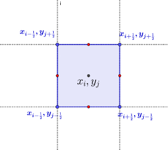
Figure 7: Illustration of the notation related to the ,$(i,j)$-cell.

The pair $(x_{i}^{n},y_{j}^{n})$ is the centers of the $(i,j)$-cell, $i,j\in\mathds{Z}$. From now on, for short, when there is no chance of misunderstanding, the limits of integration will indicate the time level where integration calculation takes place with respect to the pair $(x_{i},y_{j})$ of the $(i,j)$-cell, $i,j\in\mathds{Z}$. In each cell $\left[x_{i-\frac{1}{2}}^{n},x_{i+\frac{1}{2}}^{n}\right]\times\left[y_{j-\frac{1}{2}}^{n},y_{j+\frac{1}{2}}^{n}\right]$ (see Figure 7), the approximate solution for (21), is defined by

(23) $$U(x_{i},y_{j},t^{n})=U_{i,j}^{n}\equiv\frac{1}{\Delta x\Delta y}\int_{x_{i-\frac{1}{2}}^{n}}^{x_{i+\frac{1}{2}}^{n}}\int_{y_{j-\frac{1}{2}}^{n}}^{y_{j+\frac{1}{2}}^{n}}u(x,y,t^{n})\,dx\,dy,$$

(24) $$\overline{U}(x_{i},y_{j},t^{n+1})=\overline{U}_{i,j}^{n+1}\equiv\frac{1}{h_{x,i}^{n+1}h_{y,j}^{n+1}}\int_{\overline{x}_{i-\frac{1}{2}}^{n+1}}^{\overline{x}_{i+\frac{1}{2}}^{n+1}}\int_{\overline{y}_{j-\frac{1}{2}}^{n+1}}^{\overline{y}_{j+\frac{1}{2}}^{n+1}}u(x,y,t^{n+1})\,dx\,dy,$$

along with the initial condition $U(x_{i}^{0},y_{j}^{0},t^{0})=U_{i,j}^{0}$ in the cells $\left[x_{i-\frac{1}{2}}^{0},x_{i+\frac{1}{2}}^{0}\right]\times\left[y_{j-\frac{1}{2}}^{0},y_{j+\frac{1}{2}}^{0}\right]$, $i,j\in\mathds{Z}$. It is worthy to mention that the approximation value $\overline{U}(x_{i},y_{j},t^{n+1})$ is performed over the region $\overline{R}_{i,j}^{n+1}$; see the right picture in Figure 10 as well as Figure 11, for an illustration of the projection procedure over original grid in control volumes. Note that in (23) and (24), the quantity $u(x,y,t)$ is a solution of (21). The discrete counterpart of the space $L^{p}(\mathds{R}^{2})$ is $l_{\Delta x,\Delta y}^{p}$, the space of sequences $U=(U_{i,j})$, with $i,j\in\mathds{Z}$, with norm given by

$$\|U\|_{l_{\Delta x,\Delta y}^{p}}=\left(\Delta x\Delta y\sum_{i\in\mathds{Z}}\sum_{j\in\mathds{Z}}|U_{i,j}|^{p}\right)^{\frac{1}{p}},\quad\text{ where }1\leq p<\infty.$$

To build the new two dimensional scheme we extend the concept of no flow surface region $D_{ij}^{n}$ (see [17, 18]) to three dimensional variables ($x$,$y$ and $t$) as $D_{i,j}^{n}\subset\mathds{R}^{3}$, where $i$ and $j$ refer to $(x_{i},y_{j})$ and $n$ refers to time state $t^{n}$. The border of the control volume $D_{i,j}^{n}$ is represented by $\partial D_{i,j}^{n}=R_{i,j}^{n}\cup S_{i,j}^{n}\cup\overline{R}_{i.j}^{n+1}$ where (see Figure 7),

• $R_{i,j}^{n}=\left[x_{i-\frac{1}{2}}^{n},x_{i+\frac{1}{2}}^{n}\right]\times\left[y_{j-\frac{1}{2}}^{n},y_{i+\frac{1}{2}}^{n}\right]$ in $\mathds{R}^{2}$ is the entry of the no flow surface region

• $\overline{R}_{i,j}^{n+1}=\left[\overline{x}_{i-\frac{1}{2}}^{n+1},\overline{x}_{i+\frac{1}{2}}^{n+1}\right]\times\left[\overline{y}_{j-\frac{1}{2}}^{n+1},\overline{y}_{i+\frac{1}{2}}^{n+1}\right]$ is the exit of the no flow sufarce region, and

• $S_{i,j}^{n}$, in $\mathds{R}^{3}$, is the lateral surface of the no flow surface region.

We consider now (21) in the generalized space-time divergence form,

(25) $$\nabla_{t,x,y}\left[\begin{array}[]{c}u\\ f(u)\\ g(u)\end{array}\right]=0.$$

Integration over the control volume and the use of the divergence theorem gives,

(26) $$\int_{{\color[rgb]{0,0,0}\partial D_{i,j}^{n}}}\left[\begin{array}[]{c}u\\ f(u)\\ g(u)\end{array}\right]\cdot\vec{\textsl{n}}\,\,d(\partial D_{i,j}^{n})=0.$$

The normal vector in the entry of the no flow surface region, $R_{i,j}^{n}$, is $\left[-1\,\,0\,\,0\right]^{T}$ and the vector normal in the exit of the no flow surface region, $\overline{R}_{i,j}^{n+1}$, is $\left[1\,\,0\,\,0\right]^{T}$. Then, the right side of (26) can be written as

(27) $$\int_{R_{i,j}^{n}}\left[\begin{array}[]{c}u\\ f(u)\\ g(u)\end{array}\right]\cdot\left[-1\,\,0\,\,0\right]^{T}\,\,dA+\int_{S_{i,j}^{n}}\left[\begin{array}[]{c}u\\ f(u)\\ g(u)\end{array}\right]\cdot\vec{\textsl{n}}\,\,dS+\int_{\overline{R}_{i,j}^{n+1}}\left[\begin{array}[]{c}u\\ f(u)\\ g(u)\end{array}\right]\cdot\left[1\,\,0\,\,0\right]^{T}\,\,dA=0.$$

We assume there is not flow through the surface $S_{i,j}^{n}$ (that is, $S_{i,j}^{n}$ is impervious; this is natural in many applications [17, 18, 19, 20, 22]). Therefore surface integral of $S_{i,j}^{n}$ is zero, i.e.,

(28) $$\int_{\overline{R}_{i,j}^{n+1}}u(x,y,t^{n+1})\,\,dA=\int_{R_{i,j}^{n}}\,\,u(x,y,t^{n})\,\,dA,$$

which we call conservation identity. The numerical approximations $U_{i,j}^{n}$ and $\overline{U}_{i,j}^{n+1}$ appearing in (23) and (24), respectively, can be defined from equation (28) with the desired conservation properties and reads,

(29) $$\overline{U}_{i,j}^{n+1}=\frac{1}{\overline{R}_{i,j}^{n+1}}\int_{\overline{R}_{i,j}^{n+1}}u(x,y,t^{n+1})\,\,dA=\frac{R_{i,j}^{n}}{\overline{R}_{i,j}^{n+1}}\frac{1}{R_{i,j}^{n}}\int_{R_{i,j}^{n}}\,\,u(x,y,t^{n})\,\,dA={\color[rgb]{0,0,0}\frac{R_{i,j}^{n}}{\overline{R}_{i,j}^{n+1}}}U_{i,j}^{n}.$$

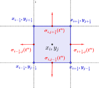
Figure 8: Normal vectors on each side of $R_{i,j}^{n}$-cell (left). No flow surface region and parametrized curves from time level $t^{n}$ to $t^{n+1}$ (right).

On other hand, from (25) and by the natural conservation properties of the no flow surface region for hyperbolic conservation law it follows

(30) $$\int_{S_{i,j}^{n}}\left[\begin{array}[]{c}u\\ f(u)\\ g(u)\end{array}\right]\cdot\vec{\textsl{n}}\,\,dS=0\qquad\text{ and }\qquad\left[\begin{array}[]{c}u\\ f(u)\\ g(u)\end{array}\right]\cdot\vec{\textsl{n}}=0.$$

Now, let ${\color[rgb]{0,0,0}\sigma_{i-\frac{1}{2},j}^{n}(t)}=(t,\sigma_{1}(t),\sigma_{2}(t))$, $t^{n}\leq t<t^{n}$, be a parametrized curve such that

$${\color[rgb]{0,0,0}\sigma_{i-\frac{1}{2},j}^{n}(t^{n})}=(t^{n},\sigma_{1}(t^{n}),\sigma_{2}(t^{n}))=(t^{n},x_{i-\frac{1}{2}},y_{j})$$

and ${\color[rgb]{0,0,0}\sigma_{i-\frac{1}{2},j}^{n}(t)}\in S_{i,j}$. Analogously, we can define parameterized curves correspoding to other sides of $R_{i,j}^{n}$ such that ${\color[rgb]{0,0,0}\sigma_{i+\frac{1}{2},j}^{n}(t),\sigma_{i,j-\frac{1}{2}}^{n}(t),\sigma_{i,j+\frac{1}{2}}^{n}(t)}\in S_{i,j}$ with initial point ($t=t^{n}$) in the respective center of the side of $R_{i,j}^{n}$ (see Figure 8).

Construction of a lateral curve of the no flow surface region. First, such construction is not unique. Actually, this might lead to a family of methods; this interesting issue will not be addressed in this work. Make fixed the point ${\color[rgb]{0,0,0}\sigma_{i-\frac{1}{2},j}^{n}(t^{n})}$. The normal vector to the corresponding side of $R_{i,j}^{n}$ is the vector $\left[t^{n},-1,0\right]^{T}$. Moreover, the normal vector on the curve ${\color[rgb]{0,0,0}\sigma_{i-\frac{1}{2},j}^{n}(t)}$ at $t^{n}\leq t<t_{n1}$ is a orthogonal vector to vector ${\color[rgb]{0,0,0}(\sigma_{i-\frac{1}{2},j}^{n})^{\prime}(t)}=\left[1,\sigma_{1}^{\prime}(t),0\right]$; see right frame in Figure 8. Indeed, the vector at point ${\color[rgb]{0,0,0}\sigma_{i-\frac{1}{2},j}^{n}(t)}$ may be calculated as $n=\left[-1,\frac{1}{\sigma_{1}^{\prime}(t)},0\right]$ and follows:

(31) $$0=\left[u\,\,\,f(u)\,\,\,g(u)\right]^{T}\cdot\vec{\textsl{n}}=\left[u\,\,\,f(u)\,\,\,g(u)\right]^{T}\cdot\left[-1,\frac{1}{\sigma_{1}^{\prime}(t)},0\right]=-u+\frac{f(u)}{\sigma_{1}^{\prime}(t)}{\color[rgb]{0,0,0}\mbox{ and then }}$$

(32) $$\sigma_{1}^{\prime}(t)=\frac{f(u)}{u}$$

with ${\color[rgb]{0,0,0}\sigma_{i-\frac{1}{2},j}^{n}(t^{n})}=(t^{n},x_{i-\frac{1}{2}},y_{j})$. Finally, since ${\color[rgb]{0,0,0}\sigma_{i-\frac{1}{2},j}^{n}(t)}$ is in the plane $y=y_{j}$, then ${\color[rgb]{0,0,0}\sigma_{i-\frac{1}{2},j}^{n}(t)}=(t,\sigma_{1}(t),y_{j})$. We point out that an analogous reasoning as in (31)-(32) might lead to the parametrized curves ${\color[rgb]{0,0,0}\sigma_{i+\frac{1}{2},j}^{n}(t)}=\left[t,\gamma_{1}(t),y_{j}\right]$, ${\color[rgb]{0,0,0}\sigma_{i,j-\frac{1}{2}}^{n}(t)}=\left[t,x_{i},\alpha_{2}(t)\right]$, ${\color[rgb]{0,0,0}\sigma_{i,j+\frac{1}{2}}^{n}(t)}=\left[t,x_{i},\theta_{2}(t)\right]$, $\gamma_{1}(t)$, such that $\alpha_{2}(t)$ and $\theta_{2}(t)$ must satisfy the exact conditions,

(33) $$\begin{array}[]{l l l}\begin{cases}\gamma_{1}(t)^{\prime}(t)\!=\!\frac{f(u)}{u},\\ \gamma_{1}(t)^{\prime}(t^{n})\!=\!(t^{n},x_{i+\frac{1}{2}},y_{j}),\end{cases}\!\!\!\!\!\!&\!\!\!\!\!\!\begin{cases}\alpha_{2}(t)^{\prime}(t)\!=\!\frac{g(u)}{u},\\ \alpha_{2}(t)^{\prime}(t^{n})\!=\!(t^{n},x_{i},y_{j-\frac{1}{2}}),\end{cases}\!\!\!\!\!\!&\!\!\!\!\!\!\begin{cases}\theta_{2}(t)^{\prime}(t)\!=\!\frac{g(u)}{u},\\ \theta_{2}(t)^{\prime}(t^{n})\!=\!(t^{n},x_{i},y_{j+\frac{1}{2}}).\end{cases}\end{array}$$

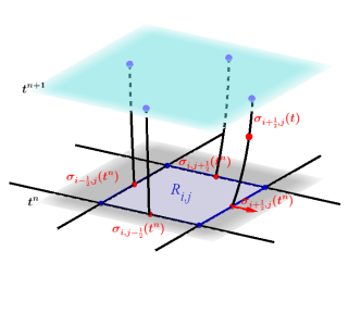
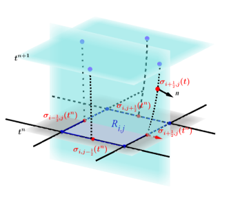
Figure 9: No flow surface region (left). Normal vector $\vec{\textsl{n}}$ in $y=y_{j}$-plane (right).

Remark: We point out that solutions for the generalized ODE system (34) to compute $\sigma_{i-1/2,j}^{n}(t)$ in Eq.(35) by the differential equation $\frac{d\sigma_{i-1/2,j}^{n}(t)}{dt}=\frac{f(U_{i-\frac{1}{2},j}^{n})}{U_{i-\frac{1}{2},j}^{n}}$ on the edge of the no flow surface region (see Figure 9 and Figure 10) can be facilitated by suitable linear resconstrution $L(x,t)$ such as $U_{i-\frac{1}{2},j}=\displaystyle\frac{1}{h}\int_{x_{i-1,j}^{n}}^{x_{i,j}^{n}}L(x,t)dx$. The situation is similar for quantities $U_{i+\frac{1}{2},j}^{n}$, $U_{i,j-\frac{1}{2}}^{n}$ and $U_{i,j+\frac{1}{2}}^{n}$; see Section 3.2 for details.

We choose the simplest approximation of system (33), by setting $U_{i,j}^{n}$ at $t=t^{n}$ we get:

(34) $$\begin{array}[]{l l l}\begin{cases}\gamma_{1}(t)^{\prime}(t)=\frac{f\left(U_{i+\frac{1}{2},j}^{n}\right)}{U_{i+\frac{1}{2},j}^{n}},\\ \gamma_{1}(t)^{\prime}(t^{n})=x_{i+\frac{1}{2}},\end{cases}\!\!\!&\!\!\!\begin{cases}\alpha_{2}(t)^{\prime}(t)=\frac{g\left(U_{i,j-\frac{1}{2}}^{n}\right)}{U_{i,j-\frac{1}{2}}^{n}},\\ \alpha_{2}(t)^{\prime}(t^{n})=y_{j-\frac{1}{2}},\end{cases}\!\!\!&\!\!\!\begin{cases}\theta_{2}(t)^{\prime}(t)=\frac{g\left(U_{i,j+\frac{1}{2}}^{n}\right)}{U_{i,j+\frac{1}{2}}^{n}},\\ \theta_{2}(t)^{\prime}(t^{n})=y_{j+\frac{1}{2}},\end{cases}\end{array}$$

where

(35) $$\frac{f(U_{i+\frac{1}{2},j}^{n})}{U_{i+\frac{1}{2},j}^{n}}\equiv f_{i+\frac{1}{2},j},\,\,\frac{f(U_{i-\frac{1}{2},j}^{n})}{U_{i-\frac{1}{2},j}^{n}}\equiv f_{i-\frac{1}{2},j},\,\,\frac{g(U_{i,j-\frac{1}{2}}^{n})}{U_{i,j-\frac{1}{2}}^{n}}\equiv g_{i,j-\frac{1}{2}}\mbox{ and }\frac{g(U_{i,j+\frac{1}{2}}^{n})}{U_{i,j+\frac{1}{2}}^{n}}\equiv g_{i,j+\frac{1}{2}}.$$

Thus, we can approximate curves of the no flow surface region at $t^{n}<t<t^{n+1}$ as:

$$\sigma_{1}(t)\approx{\color[rgb]{0,0,0}x_{i-\frac{1}{2}}}+(t-t^{n})f_{i-\frac{1}{2},j},$$

$$\gamma_{1}(t)\approx x_{i+\frac{1}{2}}+(t-t^{n})f_{i+\frac{1}{2},j},$$

$$\alpha_{2}(t)\approx y_{j-\frac{1}{2}}+(t-t^{n})g_{i,j-\frac{1}{2}},$$

and

$$\theta_{2}(t)\approx y_{j+\frac{1}{2}}+(t-t^{n})g_{i,j+\frac{1}{2}}.$$

The approximation of the volume ${\color[rgb]{0,0,0}D_{i,j}^{n}}$ gives (see right frame in Figure 10):

$${\color[rgb]{0,0,0}D_{i,j}^{n}}=\{(t,x,y)/t^{n}\leq t<t^{n+1},\,\,\,\sigma_{1}(t)\leq x<\gamma_{1}(t),\,\,\,\alpha_{2}(t)\leq y<\theta_{2}(t)\}.$$

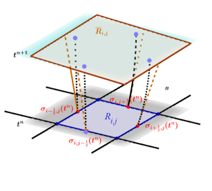
Figure 10: Analitic (left) and approximated (right) no flow surface region.

The new conservative Lagrangian-Eulerian scheme is given by very simply formulas:

STEP I (Lagrangian Evolution, see Figure 10, and below $h\equiv\Delta y=\Delta x$)

(36) $$\overline{U}_{i,j}^{n+1}=\frac{A(R_{i,j}^{n})}{A(\overline{R}_{i,j}^{n+1})}U_{i,j}^{n},\quad\text{ with }A(R_{i,j}^{n})={\color[rgb]{0,0,0}h^{2}}\text{ and }A(\overline{R}_{i,j}^{n+1})=h_{i}^{n}*h_{j}^{n}$$

where $h_{i}^{n}*h_{j}^{n}=({\color[rgb]{0,0,0}\Delta x}-(f_{i-1/2,j}+f_{i+1/2,j})\Delta t)*({\color[rgb]{0,0,0}\Delta y}-(g_{i,j-1/2}+g_{i,j+1/2})\Delta t)$.

STEP II (Eulerian Projection, see Figure 11)

(37) $${\color[rgb]{0,0,0}U_{i,j}^{n+1}}=\frac{1}{A(\overline{R}_{i,j}^{n+1})}(C1+C2+C3),$$

where $C1\equiv c_{11}\overline{U}_{i-1,j-1}^{n+1}+c_{12}\overline{U}_{i,j-1}^{n+1}+c_{13}\overline{U}_{i+1,j-1}^{n+1}$, $C2\equiv c_{21}\overline{U}_{i-1,j}^{n+1}+c_{22}\overline{U}_{i,j}^{n+1}+c_{23}\overline{U}_{i+1,j}^{n+1}$ and $C3\equiv c_{31}\overline{U}_{i-1,j+1}^{n+1}+c_{32}\overline{U}_{i,j+1}^{n+1}+c_{33}\overline{U}_{i+1,j+1}^{n+1}$.

Figure 11: Projection over original grid.

3.2 Improving numerically the solution of the generalized ODE system (34) with conservation and robustness

Solutions $\sigma_{i-1/2,j}^{n}(t)$ of the differential system can be obtained using the approximations

(38) $$\begin{array}[]{ll}U_{i-\frac{1}{2},j}&=\displaystyle\frac{1}{h}\int_{x_{i-1,j}^{n}}^{x_{i,j}^{n}}L(x,t)dx=\frac{1}{h}\left(\int_{x_{i-1,j}^{n}}^{x_{i-\frac{1}{2},j}^{n}}L_{i-1,j}(x,t)dx+\int_{x_{i-\frac{1}{2},j}^{n}}^{x_{i,j}^{n}}L_{i,j}(x,t)dx\right)\\ \\ &=\displaystyle\frac{1}{2}(U_{i-1,j}+U_{i,j})+\frac{1}{8}(U^{\prime}_{i,j}-U^{\prime}_{i-1,j}).\end{array}$$

Additional and even high-order approximations are also acceptable for $\frac{d\sigma_{j-1/2}^{n}(t)}{dt}=\frac{f(u)}{u}$ (see (34)). As in [23], the piecewise constant numerical data is reconstructed into a piecewise linear approximation through the use of MUSCL-type interpolants: $L_{i,j}(x,t)=u_{i,j}(t)+(x-x_{j})\frac{1}{\Delta x}u^{\prime}_{i,j}$. For the numerical derivative $\frac{1}{\Delta x}u^{\prime}_{i,j}$, there are several choices of slope limiters for scalar case; in the book [93] there is a good compilation of many possible options. Finally, in order to show the flexibility of the reconstruction we use the nonlinear Lagrange polynomial in $U_{i-1,j}^{n}$, $U_{i,j-1}^{n}$, $U_{i,j}^{n}$, $U_{i,j+1}^{n}$ and $U_{i+1,j}^{n}$. Therefore, equation (36) reads

(39) $$\overline{U}_{i,j}^{n+1}=\displaystyle\frac{1}{h_{j}^{n}}\displaystyle\int_{s_{j-\frac{1}{2}}^{n}}^{s_{j+\frac{1}{2}}^{n}}P_{2}(x,y)ds,$$

where $s=x,y$ and $P_{2}(x,y)=U_{i-1,j}^{n}\,L_{-1}(x-x_{i})+U_{i,j-1}^{n}\,L_{-1}(y-y_{j})+U_{i,j}^{n}\,L_{0}(x-x_{i})+U_{i,j}^{n}\,L_{0}(y-y_{j})+U_{i+1,j}^{n}\,L_{1}(x-x_{j})+U_{i,j+1}^{n}\,L_{1}(y-y_{j})$ and

(40) $$L_{\pm\,1}(x)=\frac{1}{2}\left[\left(\frac{x}{h}\pm\frac{1}{2}\right)^{2}-\frac{1}{4}\right],\quad\quad\quad L_{0}(x)=1-\left(\frac{x}{\Delta x}\right)^{2}.$$

3.3 A Lagrangian-Eulerian CFL stability constraint

Next, by definition of $f_{i-1/2,j}$, $f_{i+1/2,j}$, $f_{i,j-1/2}$ and $f_{i,j+1/2}$ in (34), we obtain the resulting coefficients of the Eulerian projection formula (37) as follows. Let the vectors

$$C_{x}=\left[C_{xl},{\color[rgb]{0,0,0}\Delta x}-C_{xl}-C_{xr},C_{xr}\right],$$

where $C_{xl}=0.5(1+\mbox{sign}(f_{i-1/2,j}))f_{i-1/2,j}\Delta t$, $C_{xr}=0.5(1-\mbox{sign}(f_{i+1/2,j}))f_{i+1/2,j}\Delta t$ and

$$C_{y}=\left[C_{yr},{\color[rgb]{0,0,0}\Delta y}-C_{yr}-C_{yr},C_{yr}\right],$$

where $C_{yl}=0.5(1+\mbox{sign}(g_{i,j-1/2}))g_{i,j-1/2}\Delta t$, $C_{yr}=0.5(1-\mbox{sign}(g_{i,j+1/2}))g_{i,j+1/2}\Delta t$.

We define the coefficients of projection formula (37) as the coefficients of the matrix

(41) $$C=(c_{i,j})=C_{x}^{T}C_{y},$$

under the CFL-condition (along with $h\equiv\Delta x=\Delta y$)

(42) $$\max_{i,j}\{{\color[rgb]{0,0,0}\left|f^{\prime}(U_{i,j}^{n})\right|},{\color[rgb]{0,0,0}\left|g^{\prime}(U_{i,j}^{n})\right|},\left|f_{i-1/2,j}\right|,\left|f_{i+1/2,j}\right|,\left|g_{i,j-1/2}\right|,\left|g_{i,j+1/2}\right|\}\Delta t<\frac{{\color[rgb]{0,0,0}h}}{2}.$$

3.4 A connection with monotone convergent entropy stable numerical scheme

For the purpose of this work, we invoke the solid theory of general monotone difference schemes (see, e.g., [64, 65, 48, 57]) to illustrate the generality or our Lagrangian-Eulerian approach (36)-(37), under the CFL stability constraint (42). By definition of matrix,

(43) $$A_{i,j}=\left[\begin{array}[]{lll}\overline{U}_{i-1,j-1}^{n+1}&\overline{U}_{i,j-1}^{n+1}&\overline{U}_{i+1,j-1}^{n+1}\\ \overline{U}_{i-1,j}^{n+1}&\overline{U}_{i,j}^{n+1}&\overline{U}_{i+1,j}^{n+1}\\ \overline{U}_{i-1,j+1}^{n+1}&\overline{U}_{i,j+1}^{n+1}&\overline{U}_{i+1,j+1}^{n+1}\end{array}\right],$$

the Eulerian Projection step (37) over original grid may be recast as

(44) $$U_{i,j}^{n+1}=C_{x}A_{i,j}^{T}C_{y}^{T},$$

or in the form of conservative monotone scheme as,

(45) $$U_{i,j}^{n+1}=U_{i,j}^{n}-\lambda^{x}\Delta_{+}^{x}F(U_{i-p,i-r}^{n},...,U_{i+q+1,j+s+1}^{n})-\lambda^{y}\Delta_{+}^{y}G(U_{i-p,j-r}^{n},...,U_{i+q+1,j+s+1}^{n})$$

where, along with (36) and taking $h=\Delta x=\Delta y$, we have,

• $F(U_{i-1,j-1}^{n},...,U_{i+1,j+1}^{n})=$

• $F_{R}(U_{i,j-1}^{n},U_{i-1,j-1}^{n},U_{i-1,j}^{n},U_{i,j}^{n},U_{i,j-1}^{n})-F_{L}(U_{i-1,j+1}^{n},,U_{i-1,j}^{n},U_{i,j-1}^{n},U_{i,j}^{n},U_{i,j+1}^{n}),$

where

• $F_{R}=h_{y}C_{xl}\left(\overline{U}_{i+1,j}^{n+1}-\overline{U}_{i,j}^{n+1}\right)-$

• $C_{xl}C_{yr}\left(\overline{U}_{i-1,j+1}^{n+1}-\overline{U}_{i-1,j}^{n+1}-(\overline{U}_{i,j+1}^{n+1}-\overline{U}_{i,j}^{n})\right)+\frac{1}{2}(f(U_{i-1,j}^{n})+f(U_{i+1,j}^{n})),$

• $F_{L}=h_{y}C_{xl}C_{yl}\left(\overline{U}_{i-1,j}^{n+1}-\overline{U}_{i,j}^{n+1}\right)-$

• $C_{xl}C_{yl}\left(\overline{U}_{i-1,j-1}^{n+1}-\overline{U}_{i,j-1}^{n+1}-(\overline{U}_{i-1,j}^{n+1}-\overline{U}_{i,j}^{n+1})\right)+\frac{1}{2}(f(U_{i-1,j}^{n})+f(U_{i+1,j}^{n})).$

and

• $G(U_{i-1,j-1}^{n},...,U_{i+1,j+1}^{n})=$

• $G_{R}(U_{i-1,j}^{n},U_{i,j}^{n},U_{i+1,j+1}^{n},U_{i,j+1}^{n},U_{i+1,j}^{n})-G_{L}(U_{i+1,j}^{n},,U_{i,j}^{n},U_{i,j-1}^{n},U_{i+1,j}^{n},U_{i,j+1}^{n}),$

• $G_{R}=h_{x}C_{yl}\left(\overline{U}_{i,j+1}^{n+1}-\overline{U}_{i,j}^{n+1}\right)-$

• $C_{xr}*C_{yl}\left(\overline{U}_{i+1,j-1}^{n+1}-\overline{U}_{i+1,j}^{n+1}-(\overline{U}_{i,j-1}^{n+1}-\overline{U}_{i,j}^{n+1})\right)+\frac{1}{2}(g(U_{i,j-1}^{n})+g(U_{i,j+1}^{n})),$

• $G_{L}=h_{x}C_{yl}\left(\overline{U}_{i,j-1}^{n+1}-\overline{U}_{i,j}^{n+1}\right)-$

• $C_{xr}*C_{yr}\left(\overline{U}_{i+1,j+1}^{n+1}-\overline{U}_{i+1,j}^{n+1}-(\overline{U}_{i,j+1}^{n+1}-\overline{U}_{i,j}^{n+1})\right)+\frac{1}{2}(g(U_{i,j-1}^{n})+g(U_{i,j+1}^{n})).$

We can note that, $F$ and $G$ satisfy condition (46), this implies consistentcy with (21) and thus the numerical method to 2D-hyperbolic equations is monotone.

In order for the above scheme be consistent with (21), we must have:

(46) $$F_{1}(u,u,...,u)=f(u)\quad\text{and}\quad F_{2}(u,u,...,u)=g(u),\quad u\in\mathds{R}.$$

Here, the functions $F_{1}$ and $F_{2}$, are the corresponding numerical fluxes of the perninent approximation. The difference approximation is monotone on the interval $\left[a,b\right]$ if $\mathcal{G}$ a nondecreasing function of each argument $U_{i,j}^{n}$ so long as all arguments lie in $\left[a,b\right]$. Write $u(x,y,t)=(S(t)u0)(x,y)$, where $S(t):L^{1}(\mathds{R}^{2})\cap L^{\infty}(\mathds{R}^{2})\rightarrow L^{1}(\mathds{R}^{2})\cap L^{\infty}(\mathds{R}^{2})$ for each $t\geq 0$ and $t\rightarrow S(t)u_{0}$ is continuous into $L^{1}(\mathds{R}^{2})$. To compute this solution numerically we set

(47) $$u^{\Delta\,t}=\sum_{n=0}^{\infty}\sum_{k=-\infty}^{\infty}U_{j,k}^{n}\,\mathcal{X}_{j,k}^{n},$$

where $\mathcal{X}_{j,k}^{n}$ is the characteristic function in the respective cell. Indeed, it turns out that conservative monotone schemes converge to entropy solutions. Therefore, convergence toward the entropy solution to out our Lagrangian-Eulerian approach (36)-(37) is proven. In [22], we were able to establish entropy convergence and error estimates for conservative Lagrangian-Eulerian method on triangular grids.

3.5 Numerical experiments with the Lagrangian-Eulerian with conservation properties

We present a benchmark comprehensive set of numerical tests which explore the role of accuracy of our new 2D Lagrangian-Eulerian scheme with conservation properties.

3.5.1 A numerical convergence study for a linear 2D advection flow model

First, let us consider the following initial value problem

(48) $$\frac{\partial u}{\partial t}+\frac{\partial u}{\partial x}+\frac{\partial u}{\partial y}=0,\quad\hbox{ in the computational domain }\quad(x,y,t)\in\left[0,1\right]\times\left[0,1\right]\times\left[0,1\right],$$

and initial condition,

(49) $$u(x,y,0)=\sin(\pi(x+y)).$$

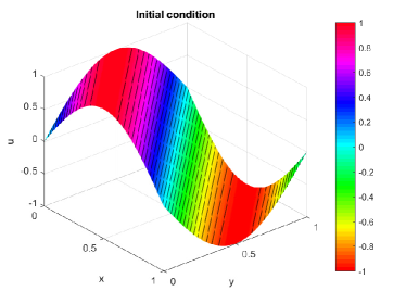
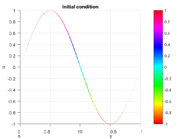
Figure 12: Initial condition for problem (48)-(49). On the left (resp. right) picture we show a “3D-plot’s view angle” (resp. a oblique projection over the plane $x=y$).

It is easy exercise to show that the exact solution to problem (48)-(49) is $u(x,y,t)=\sin(\pi(x+y-2t))$. The solution will be advanced from $t=0$ to $t=1$ and we notice that at this time the solution is merely traslated by one period $2\pi$, with respect to (49) in the oblique $x=y$ direction. The approximation computed with our scheme to problem (48)-(49) is shown in the Figure 13 (left frame) along with the exact solution on the right frame.

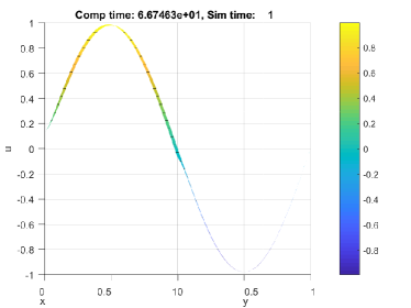
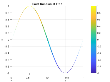
Figure 13: Computed solution by our 2D Lagrangian-Eulerian scheme (36)-(37), under the CFL stability constraint (42) to problem (48)-(49) at simulation time $t=1$ (left) and exact solution (right) both projected over oblique plane $x=y$.

In Figure 14 we observe numerical convergence rates to (48)-(49) in the $l_{h}^{1}$-norm (left), in the $l_{h}^{2}$-norm (middle) and in the $l_{h}^{\infty}$-norm (right) computed by scheme (36)-(37).

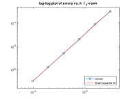
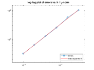
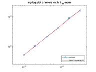
Cells	$h$	$\|u-U\|_{l_{h}^{1}}$	Order	$\|u-U\|_{l_{h}^{2}}$	Order	$\|u-U\|_{l_{h}^{\infty}}$	Order
$64\times 64$	$0.016$	$5.156\times 10^{-2}$	–	$5.573\times 10^{-2}$	–	$1.339\times 10^{-1}$	–
$128\times 128$	$0.007$	$2.046\times 10^{-2}$	$1.333$	$2.493\times 10^{-2}$	$1.161$	$6.509\times 10^{-2}$	$1.040$
$256\times 256$	$0.004$	$1.309\times 10^{-2}$	$0.644$	$1.467\times 10^{-2}$	$0.765$	$3.761\times 10^{-2}$	$0.791$
$512\times 512$	$0.002$	$6.090\times 10^{-3}$	$1.103$	$7.034\times 10^{-3}$	$1.061$	$1.835\times 10^{-2}$	$1.036$
LSF $E(h)$		$2.911*h^{0.989}$		$3.051*h^{0.972}$		$6.534*h^{0.939}$

Figure 14: In the table are shown errors between the numerical approximations ($U$) and exact solutions ($u$) in $l_{h}^{1}$, $l_{h}^{2}$ and $l_{h}^{\infty}$ norms to problem (48) with initial condition $u(x,0)=\sin(\pi(x+y))$, advanced from $t=0$ to $t=1$ along with CFL condition $0.67$.

3.5.2 An oblique Riemann problem for inviscid 2D Burgers’s equation

We consider the 2D initial value problem for the inviscid Burgers’s equation as proposed in [85],

(50) $$\frac{\partial u}{\partial t}+\frac{\partial}{\partial x}\left(\displaystyle\frac{u^{2}}{2}\right)+\frac{\partial}{\partial y}\left(\frac{u^{2}}{2}\right)=0,$$

where $(x,y,t)\in\left[0,1\right]\times\left[0,1\right]\times\left[0,0.5\right]$, and with the oblique Riemann data,

(51) $$u(x,y,0)=\begin{cases}-1.0,&x>0.5,\,\,y>0.5,\\ -0.2,&x<0.5,\,\,y>0.5,\\ 0.5,&x<0.5,\,\,y<0.5,\\ 0.8,&x>0.5,\,\,y<0.5,\\ \end{cases}$$

in conjuntion with exact boundary condition on the inflow portions of $\partial\Omega$. The correct entropic numerical solution is advanced from $t=0$ to $t=\frac{1}{12}$ as in [49] (see Figure 16).

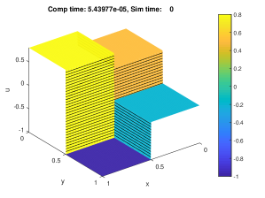
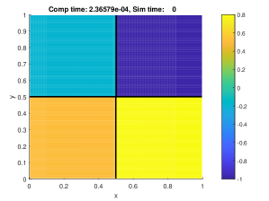
Figure 15: Initial Condition

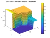
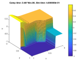
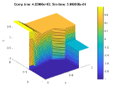
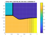
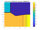
Figure 16: In top Figure are shown 3D numerical approximations with 128 x 128 to 1024 x 1024 size grid respectively, in down respectively projections over $xy$-plane.

3.5.3 A Buckley-Leverett’s problem with gravity

We consider the reservoir flow model for two-phase water-oil immiscible incompressible fluid with gravity [49],

(52) $$-\nabla\cdot\left[{\bf K}\lambda_{tot}(S_{w})\nabla p\right]=q_{tot},$$

(53) $$\frac{\partial\phi\,S_{w}}{\partial t}+\frac{\partial(u_{tot}f(S_{w}))}{\partial x}+\frac{\partial(v_{tot}g(S_{w}))}{\partial y}=q_{w},$$

where ${\bf K}$ is the absolute permeability tensor, $\lambda_{tot}$ is the total mobility, $p$ is the thermodynamic pressure, $\phi$ is the porosity, $S_{w}\in\left[0,1\right]$, $S_{w}$ is the water saturation, and ${\bf u}_{tot}=(u_{tot},v_{tot})$ is the total velocity (i.e., ${\bf u}_{tot}=u_{w}+u_{o}$). The pressure equation (52) as written is elliptic in the absence of compressibility and reads $-\nabla\cdot\left[{\bf K}\lambda_{tot}(S_{w})\nabla p\right]=0$. Because the total mobility depends of saturation, the pressure yields fields changes as the displacement evolves, this is just a statement of Darcy’s law combined with the conservation of mass. Once the pressure is computed from (52), the total velocity is given by Darcy’s law: $u_{tot}=-{\bf K}\lambda_{tot}(S_{w})\nabla p$. The equation (53) is referred to as the saturation equation. Finally, in the absence of gravity and capillarity effects the $x$- and $y$-direction flux functions $f(S_{w})$ and $g(S_{w})$ are both just the fractional flow function of water, i.e., the non-convex Buckley-Leverett flux:

(54) $$g(S_{w})=f(S_{w})=\displaystyle\frac{S_{w}^{2}}{S_{w}^{2}+\frac{\mu_{w}}{\mu_{0}}(1-C_{g}(1-S_{w})^{2})},$$

here $\mu_{w}$ and $\mu_{o}$ are the water and oil phase viscosities, respectively. For simplicity, in the simulations discussed here, we have chosen the following values of the parameters: K is the $2$ identity matrix, $\lambda_{tot}(S_{w})=1$, $\phi=1$, $q_{tot}=q_{w}=0$. Generally, the complet solution of the system (53) and (52) is obtained by the implicit method to the pressure equation (52) and the explicit method by the hyperbolic equation such approach is called an Implicit Pressure Explicit saturation (IMPES) sequential solver.

In this example, we consider the Buckley-Leverett problem with gravity proposed in [49] under the above assumptions with ${\bf u}_{tot}=(1,1)$. The equations are significantly more challenging when gravitational effects are included in the saturation equation, resulting in different (non-convex) flux functions in the $x$- and $y$-directions. In this case, $f(\cdot)$ once again the Buckley-Leverett flux (Flow), but for the flux in the $y$-direction we have,

(55) $$g(S_{w})=f(S_{w})(1-C_{g}(1-S_{w})^{2}).$$

(56) $$\frac{\partial S_{w}}{\partial t}+\frac{\partial(f(S_{w}))}{\partial x}+\frac{\partial(g(S_{w}))}{\partial y}=0,$$

with $(x,y,t)\in\left[-1.5,1.5\right]\times\left[-1.5,1.5\right]\times\left[0,0.5\right]$, and initial condition,

(57) $$u(x,y,0)=\begin{cases}1,&x^{2}+y^{2}<0.5,\\ 0,&\hbox{ otherwise}.\end{cases}$$

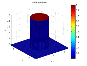
Figure 17: Initial condition flow with gravity.

Finally, we notice that we impose the solid wall (slip) boundary condition ${\bf u}_{tot}\cdot n=0$, everywhere on the boundary $\partial_{\Omega}$, where $n$ is the outward unit normal to $\partial\Omega$, upon the system (52) and (53). This means that there are no inflow boundaries and, hence, no boundary conditions on $S_{w}$. Here we have two situations we want to test our Eulerian-Lagrangian scheme: (1) a rudimentar test to address the issue of grid orientation effects (this anomalous phenomenon is observed when computational grid is rotated and substantially different numerical solutions are obtained for a same problem) and (2) accommodation of no flow boundary condition, exact or approximate. Finally, we see our numerical solutions shown in Figure 18 for the Buckley-Levertt’s problem described above (52)-(57) are in a very good agreement with those computed solutions as in [49].

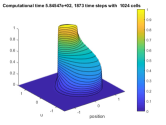
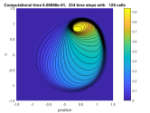
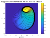
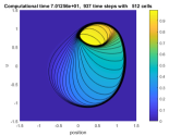
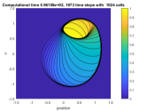
Figure 18: From top to bottom are shown the Buckley-Leverett’s numerical solutions computed with the two-dimensional scheme with respect to the reservoir waterflooding problem with gravity described in (52)-(57).

3.5.4 Conservation property verification test with scalar analytical solution velocity

In Figure 19 is shown 2D numerical solutions displayed as time evolves for a 2D symmetric Buckley-Leverett problem, in which is possible compare with exact analytical solution. Notice in top frames are shown the projection over $xu$-plane at times $T=10,110,220,340$ hours, respectively. It is clear we might see the correct front velocity of the 2D simulation being approximated with our proposed scheme when compared with the Buckley-Leverett analytical solution (superimposed red lines).

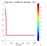
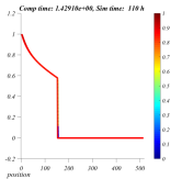
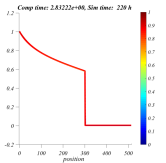
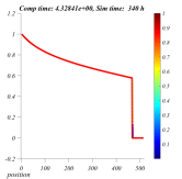
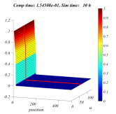
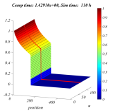
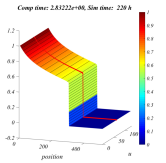
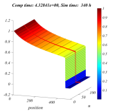
Figure 19: Conservation property verification test with scalar analytical solution velocity: projections over $xu$-plane at times $T$ = 10, 110, 220 and 430, respectively (top) and the corresponing 3D views (bottom).

4 Coupling conservative finite element method for Darcy flow problem with a locally conservative Lagrangian-Eulerian method for hyperbolic-transport

We combine a novel high-order conservative finite element method for Darcy flow problem (Section 2) with locally conservative Lagrangian-Eulerian method for hyperbolic-transport (Section 3) to address conservation properties in multiple scale in both, the complexity multiscale heterogeneity structures from rock geology appearing in the elliptic-pressure-velocity model as well as multiscale wave structures resulting from shock wave interactions from the hyperbolic-transport model.

We solve saturation and pressure equations (1)-(2) in the IMPES sequential fashion in a geological domain of $256m\times 64m$ considering two representative situations in which any one can easly reproduce further latter, namely, homogeneous medium and heterogeneous barrier and both in the slab geometry as previously described.

• Test 1 : Let’s consider an homogeneous medium ($K(x)\equiv 1$) and use the method to solve the model (1)-(2) for time from $0$ to $220$ using numerical square meshes of norms ($h_{x}=h_{y}=32,16,8,4,2,$ and $1$).

• Test 2 : Let’s consider an heterogeneous barrier medium and use the method to solve the model (1)-(2) for time from $0$ to $220$ using numerical square meshes of norms ($h_{x}=h_{y}=32,16,8,4,2$ and $1$).

For both flow situations, we present the evolution of the waves front interaction of saturation as evolve in time; see frames in Figure 20 (homogeneous medium) and 21 (heterogeneous barrier high high-constrast permability). The evolution of velocity field correponding to the heterogeneous barrier flow situation is displayed in Figure 22. Indeed, we also present the computation of the relative mass errors computed with our multiscale coupling procedure through situations Test 1 and 2, depicted in Figure 23 (homogeneous medium) and 24 (heterogeneous barrier). We also present a numerical convergence study that corroborates our findings. Based on the reported results, we were able to show the promising methodology on the conservation properties in multiple scale coupling and simulation for Darcy flow with hyperbolic-transport in complex flows.

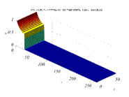
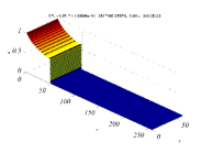
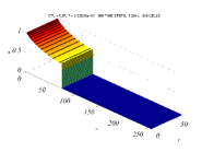
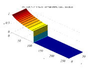
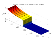
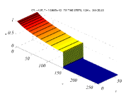
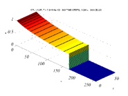
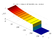
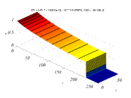
Figure 20: Evolution of saturation for Test 1 using mesh norm $h_{x}=h_{y}=1$. Solutions at times: $t=24,~{}48,~{}73,~{}97,~{}122,~{}146,~{}171,~{}195,~{}220$.

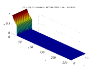
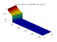
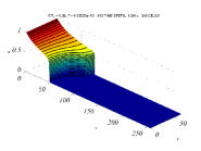
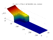
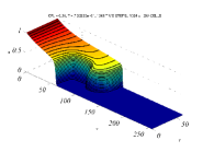
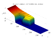
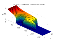
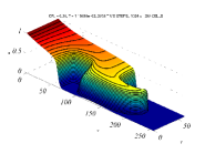
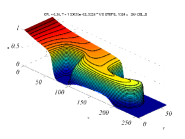
Figure 21: Evolution of saturation for Test 2 using mesh norm $h_{x}=h_{y}=1$. Solutions at times: $t=24,~{}48,~{}73,~{}97,~{}122,~{}146,~{}171,~{}195,~{}220$.

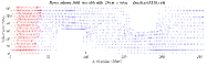
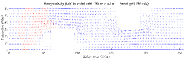
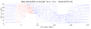
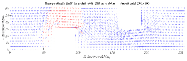
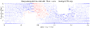
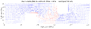
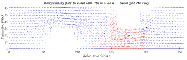
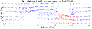
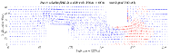
Figure 22: Evolution of velocity field for Test 2 using mesh norm $h_{x}=h_{y}=1$. Solutions at times: $t=24,~{}48,~{}73,~{}97,~{}122,~{}146,~{}171,~{}195,~{}220$.

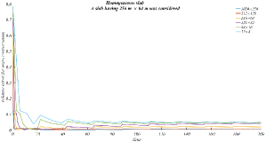
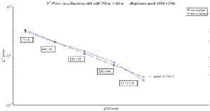
Figure 23: A 2D homogeneous slab problem coupling test for the Darcy problem with hyperbolic-transport having 256m $\times$ 64m: on the top a decreasing of the relative error of mass under a mesh refinement study and on the bottom we see evidence of numerical convergence of the full Darcy-hyperbolic-transport two-phase flow system.

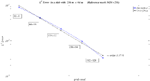
Figure 24: A 2D barrier slab problem coupling test for the Darcy problem with hyperbolic-transport having 256m $\times$ 64m: on the top a decreasing of the relative error of mass under a mesh refinement study and on the bottom we see evidence of numerical convergence of the full Darcy-hyperbolic-transport two-phase flow system.

5 Concluding remarks and perspectives

In this paper, we are concerned with modeling, simulation and numerical analysis for approximate solutions in multiscale nonlinear PDE related to highly complex problems. A better comprehension of multiscale fluid flow in subsurface is very hard, challenging and undoubtedly still of current events and demand innovative multiscale approaches, since ingenious difficulties stem from the lack of regularity of solutions. We revisited a novel volumetric locally conservative and residual-based Lagrange multipliers saddle point reformulation of the standard high-order finite method , clarifying and simplifying the presentation of its conservative properties. A new robust and accurate dynamic forward tracking Lagrangian-Eulerian scheme for hyperbolic problems do deal with multiscale wave structures resulting from shock wave interactions is also introduced. We present numerical results with realistic high-contrast two-dimensional multiscale coefficients with coupling multiscale oil-water flow simulations along with convincing numerical tests of local and global local mass conservation. We expect to combine the novel approach into the framework of Generalized Multiscale Finite Element Methods as recently introduced in [2]; see also [22] with particular interest to the case of complex flow systems as discussed in [8, 10, 12] for real-file applications, but in which issues of existence, stability properties and uniqueness are not well understood in line of works [5, 8, 12, 13, 16, 50, 67, 80].

References

- [1] J. E. Aarnes, On the use of a mixed multiscale finite element method for greater flexibility and increased speed or improved accuracy in reservoir simulation. Multiscale Model. Simul. 2(3) (2004) 421-439.
- [2] E. Abreu, C. Díaz and J. Galvis. A convergence analysis of Generalized Multiscale Finite Element Methods, Journal of Computational Physics, 396(1) (2019) 303-324.
- [3] E. Abreu, C. Díaz, J. Galvis, and M. Sarkis. On high-order conservative finite element methods, Computers & Mathematics with Applications, 75 (2018) 1852-1867.
- [4] E. Abreu, A. Espírito Santo, W. Lambert and J. Pérez, Convergence of a Lagrangian-Eulerian scheme via the weak asymptotic method, submitted.
- [5] B. Andreianov and D. Mitrović, Entropy conditions for scalar conservation laws with discontinuous flux revisited, Ann. I. H. Poincaré - AN 32 (2015) 1307-1335.
- [6] E. Abreu, M. Colombeau and E. Y. Panov, Weak asymptotic methods for scalar equations and systems. Journal of Mathematical Analysis and Applications, 444 (2016) 1203-1232.
- [7] E. Abreu, M. Colombeau and E. Y. Panov, Approximation of entropy solutions to degenerate nonlinear parabolic equations, Zeitschrift für angewandte Mathematik und Physik, 68 (2017) 133.
- [8] E. Abreu, Numerical modelling of three-phase immiscible flow in heterogeneous porous media with gravitational effects, Mathematics and Computers in Simulation, 97 (2014) 234-259.
- [9] B. Andreianov, C. Cancés. A phase-by-phase upstream scheme that converges to the vanishing capillarity solution for countercurrent two-phase flow in two-rocks media. Comput. Geosci., 18(2) (2014) 211-226
- [10] E. Abreu and D. Conceição. Numerical modeling of degenerate equations in porous media flow, Journal of Scientific Computing, 55(3) (2013) 688-717.
- [11] E. Abreu, Numerical simulation of wave propagation in three-phase flows in porous media with spatially varying flux functions. In: 4th International Conference on Hyperbolic Problems: Theory, Numerics, Applications, 2014, Padova/Itália. The proceedings of HYP2012. American Institute of Mathematical Sciences (AIMS); Series on Applied Mathematics 8 (2014) 233-240.
- [12] E. Abreu, A. Bustos, P. Ferraz and W. Lambert. A relaxation projection analytical-numerical approach in hysteretic two-phase flows in porous media, Journal of Scientific Computing 79 (2019) 1936-1980.
- [13] E. Abreu, P. Castañeda, F. Furtado and D. Marchesin. On a universal structure for immiscible three-phase flow in virgin reservoirs. Comput. Geosci. 20(1) (2016) 171-185.
- [14] E. Abreu, J. Galvis, M. Sarkis and C. Penedo. On high-order conservative finite element methods. Computers & Mathematics with Applications 75 (2018) 1852-1867.
- [15] E. Abreu, J. Galvis and C. Penedo. On high-order approximation and stability with conservative properties. Special DD24 Int. Conf. on Domain Decomposition Methods. Domain Decomposition Methods in Science and Engineering XXIV in Svalbard, Norway (Lecture Notes in Computational Science and Engineering 125) 1st ed. 2018. 2019. xxii, 570 S. 19 SW-Abb., 110 Farbabb. mm.
- [16] E. Abreu, J. Galvis and C. Penedo. A convergence analysis of Generalized Multiscale Finite Element Methods. Journal of Computational Physics, 396 (2019) 303-324.
- [17] E. Abreu and J. Perez. A fast, robust, and simple Lagrangian-Eulerian solver for balance laws and applications, Computers and Mathematics with Applications, 77(9) (2019) 2310-2336.
- [18] E. Abreu, W. Lambert, J. Perez and A. Santo. A new finite volume approach for transport models and related applications with balancing source terms, Math. Comput. Simulation 137 (2017) 2-28.
- [19] E. Abreu, J. Pérez, A. Santo. A conservative Lagrangian-Eulerian finite volume approximation method for balance law problems, Proc. Ser. Braz. Soc. Comput. Appl. Math. 5 (1) (2017) 010329-1/010329-7.
- [20] E. Abreu, J. Pérez, A. Santo. Lagrangian-eulerian approximation methods for balance laws and hyperbolic conservation laws, Rev. UIS Ing. 17 (1) (2018) 191-200, http://dx.doi.org/10.18273/revuin.v17n1-2018018, Proceeding of the XI Congreso Colombiano de Métodos Numéricos 2017.
- [21] E. Abreu, V. Matos, J. Perez and P. Rodríguez-Bermúdez. A class of Lagrangian-Eulerian shock-capturing schemes for first-order hyperbolic problems with forcing terms, submitted.
- [22] E. Abreu, J. Agudelo and J. Pérez. Convergence and error estimates for a new conservative Lagrangian-Eulerian method on triangular grids for hyperbolic conservation laws, in preparation.
- [23] E. Abreu, A. Santo and J. Pérez, Solving hyperbolic conservation laws by using Lagrangian-Eulerian approach XXXVI Congresso Nacional de Matemática Aplicada e Computacional (CNMAC), 05 a 09 de setembro de 2016, Gramado - RS.
- [24] M. Adimurthi, G.D. Veerappa Gowda, Optimal entropy solutions for conservation laws with discontinuous flux-functions. J. Hyperbolic Differ. Equ. 2(4), 783-837, pp. 2005.
- [25] G. Allaire. Homogenization and two-scale convergence. SIAM J. Math. Anal. 23(6) (1992) 1482-1518.
- [26] B. Amaziane, A. Bourgeat and M. Jurak. Effective macrodiffusion in solute transport through heterogeneous porous media. Multiscale Model. Simul. 5(1) (2006) 184-204.
- [27] B. Andreianov, K. H. Karlsen and N. H. Risebro. A Theory of -Dissipative Solvers for Scalar Conservation Laws with Discontinuous Flux, Archive for Rational Mechanics and Analysis, 201(1), 2011, pp. 27-86.
- [28] B. Andreianov. New approaches to describing admissibility of solutions of scalar conservation laws with discontinuous flux, ESAIM: ESAIM: Proceedings and Surveys, 50 2015, pp. 40-65.
- [29] B. Andreianov and C. Cancès. Vanishing capillarity solutions of Buckley-Leverett equation with gravity in two-rocks’ medium, Computational Geosciences 17 (2013) 551-572.
- [30] R. Araya, C. Harder, D. Paredes, F. Valentin. Multiscale hybrid-mixed method, SIAM Journal on Numerical Analysis 51 (6) (2013) 3505-3531 (2013).
- [31] T. Arbogast, J. Douglas and U. Hornung. Derivation of the double porosity model of single phase flow via homogenization theory. SIAM J. Math. Anal. 21(4) (1990) 823-836.
- [32] T. Arbogast, G. Pencheva, M. F. Wheeler and I. Yotov. A multiscale mortar mixed finite element method. Multiscale Model. Simul. 6(1) (2007) 319-346.
- [33] A. Azevedo, A. Souza, F. Furtado, D. Marchesin, B. Plohr, The solution by the wave curve method of three-phase flow in virgin reservoirs, Transport in Porous Media 83 (2010) 99-125.
- [34] A. Azevedo, A. Souza, F. Furtado, D. Marchesin. Uniqueness of the Riemann solution for three-phase flow in a porous medium. SIAM Journal on Applied Mathematics, 74-76 (2014) 1709-1741.
- [35] A. Azevedo, D. Marchesin, B.J. Plohr, K. Zumbrun, Capillary instability in models for three-phase flow, Zeitschrift fur Angewandte Mathematikund Physik 53 (2002) 713-746.
- [36] A. Y. Beliaev S. M. Hassanizadeh. A theoretical model of hysteresis and dynamic effects in the capillary relation for two-phase flow in porous media. Transp. Porous Media 43 (2001) 487-510.
- [37] M. Benzi, G. H. Golub, and J. Liesen. Numerical solution of saddle point problems, Acta Numer., 14 (2005) 1-137.
- [38] S. Berres, R. Burger, K.H. Karlsen, Central schemes and systems of conservation laws with discontinuous coefficients modeling gravity separation of polydisperse suspensions, Journal of Computational and Applied Mathematics (Proceedings of the 10th International Congress on Computational and Applied Mathematics) 164-165(1) (2004) 53-80.
- [39] T. Buckmaster, C. De Lellis, P. Isett and L. Székelyhidi, Jr, Anomalous dissipation for 1/5-Hölder Euler flows, Annals of Mathematics 182 (2015), 127-172.
- [40] R. Burger, K.H. Karlsen, N.H Risebro, J.D. Towers, Well-posedness in and convergence of a difference scheme for continuous sedimentation in ideal clarifier-thickener units, Numerische Mathematik 97(1) (2004) 25-65.
- [41] F. Bouchut, B. Perthame. Kružkov’s estimates for scalar conservation laws revisited, Trans. Amer. Math. Soc., 350(7) (1998) 2847-2870.
- [42] A. Bourgeat. Homogenized behavior of two-phase flows in naturally fractured reservoirs with uniform fractures distribution. Comput. Methods Appl. Mech. Eng. 47(1-2) (1984) 205-216.
- [43] K. Brenner, M. Groza, L. Jeannin, R. Masson and J. Pellerin. Immiscible two-phase Darcy flow model accounting for vanishing and discontinuous capillary pressures: application to the flow in fractured porous media, Computational Geosciences 21(5-6) (2017) 1075-1094.
- [44] C. Cancés, Asymptotic behavior of two-phase flows in heterogeneous porous media for capillarity depending only on space. II. Nonclassical shocks to model oil-trapping. SIAM J. Math. Anal. 42(2) (2010) 972-995.
- [45] M. A. Cardoso and L. J. Durlofsky. Linearized reduced-order models for subsurface flow simulation, Journal of Computational Physics 229 (2010) 681-700.
- [46] X. Cao, S. F. Nemadjieu and I. S. Pop. Convergence of an MPFA finite volume scheme for a two phase porous media flow model with dynamic capillarity. IMA J. Numer. Anal. 39 (2018) 512-544.
- [47] H. Carrillo and C. Parés. Compact Approximate Taylor Methods for Systems of Conservation Laws, Journal of Scientific Computing 80(3) (2019) 1832-1866.
- [48] C. Chainais-Hillairet. Finite volume schemes for a nonlinear hyperbolic equation. Convergence towards the entropy solution and error estimate. Mathematical Modelling and Numerical Analysis M2AN 33(1) (1999) 129-156.
- [49] I. Christov and B. Popov. New non-oscillatory central schemes on unstructured triangulations for hyperbolic systems of conservation laws. Journal of Computational Physics, 227(11) (2008) 5736-5757.
- [50] G-Q G.Chen and J. Glimm, Kolmogorov-type theory of compressible turbulence and inviscid limit of the Navier-Stokes equations in , Physica D: Nonlinear Phenomena 400(15) (2019) 132138.
- [51] G. Q. Chen and J. Glimm. Kolmogorov’s theory of turbulence and inviscid limit of the Navier-Stokes equations in R 3 . Comm. Math. Phys. 310 (1) (2012) 267-283.
- [52] Z. Chen, G. Huan and Y. Ma. Computational Methods for Multiphase Flows in Porous Media. Vol. 2. Philadelphia: SIAM (2006).
- [53] Y. Chen, L. J. Durlofsky, M. Gerritsen, X.-H Wen, A coupled local-global upscaling approach for simulating flow in highly heterogeneous formations. Adv. Water Resour. 26(10) (2003) 1041-1060.
- [54] E. Chiodaroli, C. De Lellis and O. Kreml. Global ill-posedness of the isentropic system of gas dynamics. Comm. Pure Appl. Math., 68(7) (2015) 1157-1190.
- [55] E.T. Chung, W. T. Leung, M. Vasilyeva, Y. Wang. Multiscale model reduction for transport and flow problems in perforated domains. J. Comput. Appl. Math. 330 (2018) 519-535.
- [56] M. Christie and M. Blunt. Tenth spe comparative solution project: A comparison of upscaling techniques, Society of Petroleum Engineers SPE Reservoir Simulation Symposium, 11-14 February (2001) Houston, Texas, SPE-66599-MS.
- [57] M. G. Crandall and A. Majda. Monotone difference approximations for scalar conservation laws. Mathematics of Computation, 34(149) (1980) 1-21.
- [58] G. Crasta, V. De Cicco and G. De Philippis. Kinetic Formulation and Uniqueness for Scalar Conservation Laws with Discontinuous Flux, Communications in Partial Differential Equations, 40(4) 2015, pp. 694-726.
- [59] S. Diehl. A conservation law with point source and discontinuous flux function modelling continuous sedimentation. SIAM J. Appl. Math., 56(2) (1996) 388-419.
- [60] R. J. DiPerna. Measure valued solutions to conservation laws. Arch. Rational Mech. Anal., 88(3) (1985) 223-270.
- [61] R. J. DiPerna and A. Majda. Oscillations and concentrations in weak solutions of the incompressible fluid equations. Comm. Math. Phys. 108 (4) (1987) 667-689.
- [62] L. J. Durlofsky. Numerical calculation of equivalent grid block permeability tensors for heterogeneous porous media. Water Resour. Res. 27(5) (1991) 699-708.
- [63] L. J. Durlofsky and H. Li. Local-global upscaling for compositional subsurface flow simulation. Transp. Porous Media 111(3) (2016) 701-730.
- [64] R. Eymard, T. Gallouët and R. Herbin. Existence and uniqueness of the entropy solution to a nonlinear hyperbolic equation. Chin. Ann. Math. B16 (1995) 1-14.
- [65] R. Eymard, T. Gallouët and R. Herbin. Convergence of a finite volume scheme for a nonlinear hyperbolic equation, Proceedings of the Third colloquium on numerical analysis, edited by D. Bainov and V. Covachev. Elsevier (1995) 61-70.
- [66] W. Fan, H. Sun, J. Yao, D. Fan and Y. Yang. An upscaled transport model for shale gas considering multiple mechanisms and heterogeneity based on homogenization theory. Journal of Petroleum Science and Engineering, 106392 (2019) doi:10.1016/j.petrol.2019.106392
- [67] U. S. Fjordholm, R. Käppeli, S. Mishra, and E. Tadmor. Construction of approximate entropy measure-valued solutions for hyperbolic systems of conservation laws. Found. Comput. Math., 17(3) (2017) 763-827, 2017.
- [68] U. S. Fjordholm, K. Lye, S. Mishra, F. Weber, Statistical solutions of hyperbolic systems of conservation laws: numerical approximation, https://arxiv.org/abs/1906.02536 (access in Oct 13, 2019).
- [69] H. Frid, V. Shelukhin. A Quasi-linear Parabolic System for Three-Phase Capillary Flow in Porous Media, SIAM J. Math. Anal., 35(4) (2003) 1029-1041.
- [70] H. Frid, V. Shelukhin. Initial Boundary Value Problems for a Quasi-linear Parabolic System in Three-Phase Capillary Flow in Porous Media, SIAM J. Math. Anal., 36(5) (2005) 1407-1425.
- [71] H. Florez and E. Gildin. Model-Order Reduction of Coupled Flow and Geomechanics in Ultra-Low Permeability ULP Reservoirs, SPE-193911-MS, SPE Reservoir Simulation Conference, 10-11 April, Galveston, Texas, USA 2019.
- [72] U. Frisch. Turbulence. Cambridge University Press, 1995.
- [73] F. Furtado and F. Pereira. Crossover from Nonlinearity Controlled to Heterogeneity Controlled Mixing in Two-Phase Porous Media Flows, Computational Geosciences 7(2) (2003) 115-13.
- [74] Efendiev, Yalchin, Juan Galvis, and Thomas Y. Hou. Generalized multiscale finite element methods (GMsFEM), Journal of Computational Physics 251 (2013): 116-135.
- [75] J. Galvis and M. Presho. A mass conservative generalized multiscale finite element method applied to two-phase flow in heterogeneous porous media, Journal of Computational and Applied Mathematics, 296 (2016) 376-388.
- [76] W. Ge, Q. Chang, C. Li and J. Wang. Multiscale structures in particle-fluid systems: Characterization, modeling, and simulation, Chemical Engineering Science 198(28) (2019) 198-223.
- [77] D. Groen, J. Knap, P. Neumann, D. Suleimenova, L. Veen and K. Leiter. Mastering the scales: a survey on the benefits of multiscale computing software.Phil. Trans. R. Soc. A (2019) 377: 20180147.
- [78] B. Gong, M. Karimi-Fard and L. J. Durlofsky. An upscaling procedure for constructing generalized dual-porosity/dual-permeability models from discrete fracture characterizations. SPE Annual Technical Conference and Exhibition. Society of Petroleum Engineers (2006).
- [79] R. T. Guiraldello, R. F. Ausas, F. S. Sousa, F. Pereira and G. C. Buscaglia. The multiscale Robin coupled method for flows in porous media. J. Comput. Phys. 355 (2018) 1-21.
- [80] A. G. Hoekstra , B. Chopard , D. Coster , S. P. Zwart and P. V. Coveney. Multiscale computing for science and engineering in the era of exascale performance, Phil. Trans. R. Soc. A (2019) 377: 20180144.
- [81] H. Holden, N. H. Risebro. A mathematical model of traffic flow on a network of unidirectional roads. SIAM J. Math. Anal., 26(4) (1995) 999-1017.
- [82] T. Y. Hou and X.-H. Wu. A multiscale finite element method for elliptic problems in composite materials and porous media. J. Comput. Phys. 134(1) (1997) 169-189.
- [83] J. D. Jansen and L. J. Durlofsky. Use of reduced-order models in well control optimization, Optim Eng 18 (2017) 105-132.
- [84] P. Jenny, S.H. Lee and H. A. Tchelepi. Multi-scale finite-volume method for elliptic problems in subsurface flow simulation. J. Comput. Phys. 187(1) (2003) 47-67.
- [85] G-S Jiang and E. Tadmor. Nonoscillatory central schemes for multidimensional hyperbolic conservation laws. SIAM Journal on Scientific Computing, 19(6):1892–1917, 1998.
- [86] V. V. Jikov, S. M. Kozlov and A. O. Oleinik. Homogenization of differential operators and integral functionals. Springer, Berlin Heidelberg (2012).
- [87] E. F. Kaasschieter, Solving the Buckley-Leverett equation with gravity in a heterogeneous porous medium. Comput. Geosci. 3(1) (1999) 23-48.
- [88] K. H. Karlsen, J. D. Towers, Convergence of the Lax-Friedrichs scheme and stability for conservation laws with a discontinuous space-time dependent flux. Chin. Ann. Math. Ser. B. 25(3) (2004) 287-318.
- [89] K. H. Karlsen, N. H. Risebro. Unconditionally stable methods for Hamilton-Jacobi equations. J. Comp. Phys. 180(2), 2002, pp. 710-735.
- [90] N. N. Kuznetsov. Accuracy of some approximate methods for computing the weak solutions of a first-order quasi-linear equation, USSR Comput. Math. and Math. Phys., 16 (1976), pp. 105-119.
- [91] S. H. Lee, C. Wolfsteiner and H. A. Tchelepi. Multiscale finite volume formulation for multiphase flow in porous media: black oil formulation of compressible, three-phase flow with gravity. Comput. Geosci. 12(3) (2008) 351-366.
- [92] C. De Lellis and L. Szekelyhidi, Jr. The Euler equations as a differential inclusion. Ann. of Math. (2), 170(3) (2009) 1417-1436.
- [93] R. J. LeVeque. Finite volume methods for hyperbolic problems 31. Cambridge university press, 2002.
- [94] H. Lim, Y. Yu, J. Glimm, X. L. Li and D. H. Sharp. Chaos, transport and mesh convergence for fluid mixing. Act. Math. Appl. Sin., 24 (3) (2008) 355-368.
- [95] D. Marchesin, B. Plohr. Wave structure in wag recovery, Society of Petroleum Engineering Journal 71314 (2001) 209-219.
- [96] A. Mikelić and V. Devigne and C. J. Van Duijn. Rigorous upscaling of the reactive flow through a pore, under dominant peclet and damkohler numbers. SIAM J. Math. Anal. 38(4) (2006) 1262-1287.
- [97] S. Mishra, J. Jaffré. On the upstream mobility scheme for two-phase flow in porous e media. Comput. Geosci., 14(1) (2010) 105-124.
- [98] O. Moyner and K. A. Lie. A multiscale restriction-smoothed basis method for high contrast porous media represented on unstructured grids. J. Comput. Phys. 304 (2016) 46-71.
- [99] O. Moyner and K. A. Lie. A multiscale restriction-smoothed basis method for compressible black-oil model. Society of Petroleum Engineers Journal 21(6) (2016) 2079-2096.
- [100] D. N. Ostrov. Viscosity solutions and convergence of monotone schemes for synthetic aperture radar shape-from-shading equations with discontinuous intensities. SIAM J. Appl. Math., 59(6) (1999) 2060-2085.
- [101] E. Yu. Panov, Existence of strong traces for generalized solutions of multidimensional scalar conservation laws, J. Hyperbolic Differ. Equ. 2 (2005) 885-908.
- [102] E. Yu. Panov, Existence of strong traces for quasi-solutions of multidimensional conservation laws, J. Hyperbolic Differ. Equ. 4 (2007) 729-770.
- [103] E.Yu. Panov, On existence and uniqueness of entropy solutions to the Cauchy problem for a conservation law with discontinuous flux, J. Hyperbolic Differ. Equ. 3 (2009) 525-548.
- [104] E. Yu. Panov, Existence and strong pre-compactness properties for entropy solutions of a first-order quasilinear equation with discontinuous flux, Arch. Ration. Mech. Anal. 195 (2010) 643-673.
- [105] F. A. Radu, K. Kumar, J. M Nordbotten and I. S. Pop. A robust, mass conservative scheme for two-phase flow in porous media including Hölder continuous nonlinearities. IMA J. Numer. Anal. 38(2) (2018) 884-820.
- [106] F. A. Radu, I. S. Pop and P. Knabner. Error estimates for a mixed finite element discretization of some degenerate parabolic equations. Numer. Math. 109 (2008) 285-311.
- [107] A. M. Ruf, E. Sande and S. Solem. The Optimal Convergence Rate of Monotone Schemes for Conservation Laws in the Wasserstein Distance, Journal of Scientific Computing 80 (2019) 1764-1776.
- [108] F. Sabac. The Optimal Convergence Rate of Monotone Finite Difference Methods for Hyperbolic Conservation Laws, SIAM J. Numer. Anal., 34(6) (2006) 2306-2318.
- [109] N. Seguin and J. Vovelle. Analysis and approximation of a scalar conservation law with a flux function with discontinuous coefficients, Math. Models Methods Appl. Sci. 13 (2) (2003) 221-257.
- [110] G. Singh, W. Leung and M. F. Wheeler. Multiscale methods for model order reduction of non-linear multiphase flow problems, Computational Geosciences 23 (2019) 305-323.
- [111] T. Tang. Error Estimates of Approximate Solutions for Nonlinear Scalar Conservation Laws. In: Freistühler H., Warnecke G. (eds) Hyperbolic Problems: Theory, Numerics, Applications. ISNM International Series of Numerical Mathematics, 141. Birkhäuser, Basel (2001).
- [112] A. Talonov and M. Vasilyeva. On numerical homogenization of shale gas transport. J. Comput. Appl. Math. 301 (2016) 44-52.
- [113] T. Tang and Z-h Teng. On the Regularity of Approximate Solutions to Conservation Laws with Piecewise Smooth Solutions, SIAM J. Numer. Anal., 38(5) (2006) 1483-1495.
- [114] Z-X. Tong, Y-L. He and W-Q. Tao. A review of current progress in multiscale simulations for fluid flow and heat transfer problems: The frameworks, coupling techniques and future perspectives, International Journal of Heat and Mass Transfer, 137 (2019) 1263-1289.
- [115] S. Tveit, I. Aavatsmark. Errors in the upstream mobility scheme for countercurrent two-phase flow in heterogeneous porous media, Comput Geosci 16 (2012) 809-825.
- [116] M. Vasilyeva, E. T. Chung, Y. Efendiev and J. Kim. Constrained energy minimization based upscaling for coupled flow and mechanics, Journal of Computational Physics 376(1) (2019) 660-674.
- [117] X.-H. Wu, Y. Efendiev, T. Y. Hou. Analysis of upscaling absolute permeability. Discrete and Continuous Dynamical Systems Series B 2(2) (2002) 185-204.
- [118] Wang, M., Cheung, S. W., Chung, E. T., Efendiev, Y., Leung, W. T., Wang, Y. (2019). Prediction of Discretization of GMsFEM Using Deep Learning. Mathematics, 7(5), 412.
- [119] Efendiev, Y., Galvis, J., Wu, X. H. (2009). Multiscale finite element and domain decomposition methods for high-contrast problems using local spectral basis functions.