Reassessing Dust’s Role in Forming the CMB
Abstract
The notion that dust might have formed the cosmic microwave background (CMB) has been strongly refuted on the strength of four decades of observation and analysis, in favour of recombination at a redshift . But tension with the data is growing in several other areas, including measurements of the Hubble constant and the BAO scale, which directly or indirectly impact the physics at the surface of last scattering (LSS). The universe resolves at least some of this tension. We show in this paper that—if the BAO scale is in fact equal to the acoustic horizon—the redshift of the LSS in this cosmology is , placing it within the era of Pop III star formation, prior to the epoch of reionization at . Quite remarkably, the measured values of and in this model are sufficient to argue that the CMB temperature today ought to be K, so and the baryon to photon ratio are not independent free parameters. This scenario might have resulted from rethermalization of the CMB photons by dust, presumably supplied to the interstellar medium by the ejecta of Pop III stars. Dust rethermalization may therefore yet resurface as a relevant ingredient in the universe. Upcoming high sensitivity instruments should be able to readily distinguish between the recombination and dust scenarios by either (i) detecting recombination lines at , or (ii) establishing a robust frequency-dependent variation of the CMB power spectrum at the level of across the sampled frequency range.
E-mail: fmelia@email.arizona.edu00footnotetext: John Woodruff Simpson Fellow.
Keywords cosmic microwave background; cosmological parameters; cosmology: observations; cosmology: redshift; cosmology: theory; large-scale structure
1 Introduction
Since COBE’s discovery (Mather et al., 1990) that the spectrum of the cosmic microwave background (CMB) is a near perfect blackbody, all succeeding measurements of this relic signal (including those reported in refs. Hinshaw et al. 2003; Planck Collaboration 2014) have been interpreted self-consistently in terms of a model in which the radiation was thermalized within one year of the big bang. Diffusing through a gradually thinning, scattering-dominated medium, these photons eventually streamed freely once the protons and electrons in the cosmic fluid combined to form neutral hydrogen and helium, a process (not so accurately) referred to as ‘recombination.’
The actual origin of the CMB was not always so evident, however, and serious consideration had been given to the possibility that it was produced by dust in the early Universe, injected into the interstellar medium (ISM) by Pop III stars (Rees, 1978; Rowan et al., 1979; Wright, 1982). An additional attraction of this scenario was the likelihood that the photons rethermalized by dust were themselves emitted by the same stars, thereby closing the loop on a potentially elegant, self-consistent physical picture.
But the dust model for the CMB very quickly gave ground to recombination for several telling reasons. Two of them, in particular, relied heavily on each other and suggested quite emphatically that the surface of last scattering (LSS) had to lie at a redshift . First, there was the inference of a characteristic scale in the CMB’s power spectrum (Spergel et al., 2003) which, when identified as an acoustic horizon (see below), implied that radiation must have decoupled from the baryonic fluid no more than yrs after the big bang (placing it at the aforementioned ). Second, one could reasonably assume that the CMB propagated more or less freely after this time, so that its temperature scaled as . Assuming that the radiation and matter were in thermal equilibrium prior to the LSS, one could then use the Saha equation to estimate the temperature —and hence the redshift—at which the free electron fraction dropped to , signaling the time during which the baryonic fluid transitioned from ionized plasma to neutral gas. Recombination would have occurred at K and, given a measured CMB temperature today of K, this would imply a redshift , nicely consistent with the interpretation of the acoustic scale. In contrast, emission dominated by dust at K would have placed the redshift at no more than , creating a significant conflict with the acoustic-scale interpretation of the peaks in the CMB power spectrum. And in parallel with such arguments for recombination, there was also growing concern that Pop III starlight scattered by the stars’ own ejected dust faced seemingly insurmountable difficulties accounting for the observed CMB spectrum (see, e.g., Li 2003).
Today, there is very little doubt that the CMB must have formed via recombination at in the context of CDM. A dust scenario would produce too many inconsistencies with the age-redshift relation and the Pop III star formation rate, among many other observables. As the precision and breadth of the measurements continued to improve, however, the basic recombination picture for the CMB’s origin has not remained as clear as one might have hoped two decades ago—not because of problems with the CMB itself but, rather, because of the tension this interpretation creates with other kinds of cosmological observations. For example, from the analysis of the CMB observed with Planck (Planck Collaboration 2014), one infers a value of the Hubble constant ( km s-1 Mpc-1) lower than is typically measured locally, and a higher value for the matter fluctuation amplitude () than is derived from Sunyaev-Zeldovich data. Quite tellingly, none of the extensions to the six-parameter standard CDM model explored by the Planck team was able to resolve these inconsistencies. As we shall see below, comparable tension now exists also between the baryon acoustic oscillation (BAO) scale inferred from the galaxy and quasar distributions at and the aforementioned acoustic length seen in the CMB, weakening the argument for an LSS at .
Over the past decade, the standard model’s inability to resolve such tensions, along with several inexplicable coincidences, have led to the development of an alternative Friedmann-Robertson-Walker cosmology known as the universe (Melia, 2007, 2016, 2017b; Melia & Abdelqader, 2009; Melia & Shevchuk, 2012). During this time, the predictions of have been compared with those of CDM using over 23 different kinds of data, outperforming the standard model in every case (see, e.g., Table I in Melia 2017a). We are therefore motivated to consider how the origin of the CMB might be interpreted in this alternative cosmology. Ironically, we shall find that—if the BAO and acoustic scales are the same—the redshift of the LSS in this model had to be , remarkably close to what would have been required in the original dust model. We shall also find that this redshift sits right within the period of Pop III star formation, prior to the epoch of reionization (), a likely time during which dust would have been injected into the ISM. And quite interestingly, we shall also determine that if this model is correct, knowledge of and by themselves is sufficient to argue that the CMB temperature today should be K, very close to the actual value, suggesting that the Hubble constant and the baryon to photon ratio are not independent, free parameters.
Our goal in this paper is therefore not to critique the basic recombination picture in CDM which, as noted earlier, matches the data remarkably well but, rather, to demonstrate how the (now dated) dust model for the origin of the CMB may still be viable, albeit in the context of . The growing tension between the predictions of the standard model and the ever improving observations (Melia & López-Corredoira, 2018) could certainly benefit from a reconsideration of a dust origin for the CMB. But our principal motivation for reanalyzing this mechanism is that, while recombination does not work for , the dust model is unavoidable. It is our primary goal to examine how and why this association emerges naturally in this cosmology. The analysis in this paper will show that, while dust reprocessing of radiation emitted by the same first generation stars was part of the original proposal, our improved understanding of star formation during the Pop III era precludes this possibility. Instead, the background radiation would have originated between the big bang and decoupling, similarly to the situation in CDM, but would have been reprocessed by dust prior to reionization in the context of . A critical difference between these models is that the anisotropies in the observed CMB field would therefore correspond to large-scale structure at in , instead of in the standard picture.
There are, of course, several definitive tests one may carry out to distinguish between these two scenarios, and we shall consider them in our analysis, described in detail in § VI. In this section, we shall also describe several potential shortcomings of a dusty origin for the CMB versus the current recombination picture, and we shall see how these are removed in the context of , though this would not be possible in CDM. We begin in § II with a brief status report on the model, and point to the various publications where its predictions have been tested against the data. In § III, we discuss some relevant observational issues pertaining to the CMB, including the interpretation of the acoustic horizon as the characteristic length extracted from its power spectrum. In § IV we describe the BAO scale and compare it to the acoustic horizon in § V. In this section, we also discuss why the LSS had to be at if these two scales are equal. In § VI we describe how the CMB could have originated from dust opacity in this model, and we end with an assessment of our results in §§ VII and VIII.
2 The Model
The universe has been described extensively in the literature and its predictions have been tested against many observations at high and low redshifts. This cosmology has much in common with CDM, but includes an additional ingredient motivated by several theoretical and observational arguments (Melia, 2007, 2016, 2017b; Melia & Abdelqader, 2009; Melia & Shevchuk, 2012). Like CDM, it also adopts the equation of state , with and , but goes one step further by specifying that at all times. In spite of the fact that this prescription appears to be very different from the equation of state in CDM, where , nature is in fact telling us that if we ignore the constraint and instead proceed to optimize the parameters in CDM by fitting the data, the resultant value of averaged over a Hubble time, is actually within the measurement errors. Thus, although in CDM cannot be equal to from one moment to the next, its value averaged over the age of the Universe is equal to what it would have been in all along.
This result does not prove that CDM is incomplete, but nonetheless suggests that the inclusion of the additional constraint might render its predictions closer to the data. By now, one-on-one comparisons between CDM and have been carried out for a broad range of observations, from the angular correlation function of the CMB (Melia & López-Corredoira, 2018; Melia, 2014b) and high- quasars (Melia, 2013a, 2014c) in the early Universe, to gamma-ray bursts (Wei et al., 2013) and cosmic chronometers (Melia & Maier, 2013) at intermediate redshifts and, most recently, to the relatively nearby Type Ia SNe (Wei et al., 2015). The application of model selection tools to these tests indicates that the likelihood of being ‘closer to the correct model’ is typically compared to only for CDM. And most recently, the Alcock-Paczýnski test using BAO measurements has been shown to favour over CDM at high redshifts (Melia & López-Corredoira, 2017).
There is therefore ample reason to consider the viability of the Universe, and to see how one might interpret the formation of the CMB in this model. This is one of several remaining critical tests facing the universe. We recently demonstrated that, while the angular correlation function of the CMB as measured with the latest Planck release (Planck Collaboration, 2016a) remains in tension with the predictions of CDM, it is consistent with (Melia & López-Corredoira, 2018). It is still not clear, however, whether the power spectrum itself may be fully explained in this model. This paper is an important step in that direction. A second issue is whether big bang nucleosynthesis is consistent with the constant expansion rate required in this cosmology. It has been known for several decades that a linear expansion with the physical conditions in the early CDM universe simply doesn’t work because the radiation temperature and densities don’t scale properly with redshift (Kaplinghat et al., 2000; Sethi et al., 2005). In , however, the total equation of state is the zero active mass condition , in terms of the total energy density and pressure, so the various constituents in the cosmic fluid evolve differently than those in the standard model. The situation is closer to the so-called Dirac-Milne universe (Benoit-Lévy & Chardin, 2012), which also has linear expansion, so the outlook is more promising.
In reality, the standard model has not yet completely solved big bang nucleosynthesis. The yields are generally consistent with the observed abundances for 4He, 3He, and , but 7Li is over-produced by a significant amount (Cyburt et al., 2008). This problem will go away with nucleosynthesis, which is a two-step process, first through the thermal and homogeneous production of 4He and 7Li, and then via the production of and 3He. Previous work, e.g., by Benoit-Lévy & Chardin (2012), suggests that the timeline in this model is greatly different from that in CDM. Whereas all of the burning must take place before neutrons decay in the latter, nucleosynthesis is a much slower process in the former, with a neutron pool sustained via weak interactions. The burning rate is much lower, but its duration is significantly longer, so the 4He is produced over a hundred million years instead of only 15 minutes. According to these earlier simulations, the Lithium anomaly largely disappears because the physical conditions during the nuclear burning are far less extreme than in CDM. This work is well outside the scope of the present paper, of course, but we highlight it here as one of the principal remaining problems to address with this new cosmology.
The various measures of distance and time in the universe take on very simple forms, with very few parameters (Melia, 2007; Melia & Shevchuk, 2012; Melia & Maier, 2013). In some applications, there are no parameters at all, making the analysis very straightforward, and the results relatively unambiguous. For example, the Hubble constant is , and the age is , so the age-redshift relationship is
| (1) |
And since in this cosmology, we also have
| (2) |
Given the constraint on density and pressure alluded to above, it is not difficult to show how the energy density of the various constituents must evolve with redshift in this cosmology. Putting
| (3) |
and
| (4) |
we immediately see that
| (5) |
under the assumption that and . Throughout the cosmic evolution,
| (6) |
where is the critical density and in a flat universe.
Equation (5) constrains the radiation energy density in terms of dark energy and at any epoch. At low redshifts, however, we also know that the CMB temperature ( K) translates into a normalized radiation energy density , which is negligible compared to matter and dark energy. Throughout this paper, the mass fractions , , and , are defined in terms of the current matter (), radiation (), and dark energy () densities, and the critical density . Therefore, must be in order to produce a partitioning of the constituents in line with what we see in the local Universe. With this value,
| (7) |
while
| (8) |
where, of course, , representing both baryonic and dark matter (Melia & Fatuzzo, 2016).
At the other extreme, when , it is reasonable to hypothesize that is dominated by radiation and dark energy111In the context of , we know that radiation alone cannot sustain an equation of state , so dark energy is a necessary ingredient., so that . In that case, one would have
| (9) |
and
| (10) |
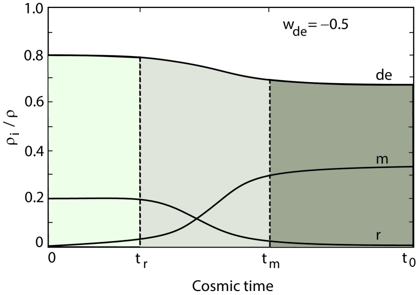
implying a relative partitioning of and (if continues to be constant at towards higher redshifts). In other words, the zero active mass condition would be consistent with a gradual transition of the equilibrium representation of the various constituents from the very early universe, in which , to the present, where . And during this evolution, the radiation energy density that is dominant at , with , would eventually have given way to matter with at later times (). This evolution is shown schematically in figure 1. As we shall see shortly, the physical properties of the medium at the LSS—presumably falling between and —provide a valuable datum in between these two extreme limits (i.e., ).

Let us now define the ratio . On the basis of the two arguments we have just made, we expect that throughout the history of the Universe. Solving Equations (3) and (4), we therefore see that, at any redshift,
| (11) |
while
| (12) |
Of course, the fact that is constrained by the expression in Equation (10) at large redshift means that the radiation is coupled to dark energy in ways yet to be determined through the development of new physics beyond the standard model. Nonetheless, for specificity, we will also assume that the radiation is always a blackbody, both at high and low redshifts, though with one important difference—that the relic photons are freely streaming below the redshift at the last scattering surface, corresponding to a time in figure 1, at which the radiation effectively ‘decouples” from the other constituents. Therefore
| (13) |
At very high redshifts, however, is given explicitly by the redshift dependence of . We still do not know precisely where the radiation decouples from matter and dark energy, and begins to stream freely according to the expression in Equation (13) but, as we shall see below, our results are not strongly dependent on this transition redshift, principally because is so narrowly constrained to the range . Thus, for simplicity, we shall assume that for we may put222In this expression, we have adopted the Planck optimized value of the Hubble constant, km s-1 Mpc-1 (Planck Collaboration 2014). To be fair, this is the value measured in the context of CDM, and while a re-analysis of the Planck data in the context of will produce a somewhat different result for , the differences are likely to be too small to affect the discussion in this paper.
| (14) |
Even before considering the consequences of identifying the BAO scale as the acoustic horizon, which we do in the next section, we can already estimate the location of the LSS by setting Equation (13) equal to (14), which yields
| (15) |
Remembering that everywhere, we therefore see that in this model must be K, no matter where the LSS is located. This is quite a remarkable result because the only input used to reach this conclusion is the value of , unlike the situation with CDM, in which one must assume both a value of and optimize the baryon to photon fraction in the early Universe to ensure a value of in this range. Figure 2 illustrates how today changes with if we assume (see below). We see that must then be when we fix K, which is consistent with being closer to than in figure 1. Indeed, we find from Equations (11) and (14) that, at , and .
We shall consider the more specific constraints imposed by the CMB acoustic horizon and the BAO peak measurements shortly, but for now we have already demonstrated a very powerful property of the universe—that and the baryon to photon ratio are not independent of each other. And clearly, while in CDM, the LSS must occur at a much lower redshift () in this model.
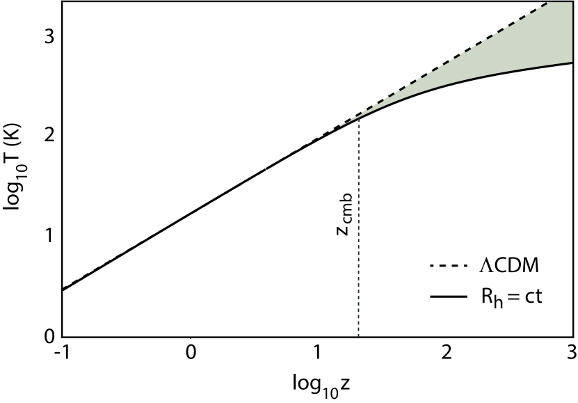
The temperature calculated from Equations (13) and (14) is compared to that of the standard model in figure 3. This figure also indicates the location of based on the argument in the previous paragraph, which will be bolstered shortly with constraints from the acoustic and BAO scales. Thus, while K at in CDM, so that hydrogen ‘recombination’ may be relevant to the CMB in this model, the temperature is too low at for this mechanism to be responsible for liberating the relic photons in .
In this regard, our reconsideration of dust’s contribution to the formation of the CMB deviates from the original proposal (Rees, 1978), in that the radiation being rethermalized at in this picture need not all have been emitted by Pop III stars. Indeed, given that for , these photons were more likely produced during the intervening period between the big bang and decoupling prior to the reprocessing by dust at . The implied coupling between radiation and the rest of the cosmic fluid at high redshifts requires physics beyond the standard model, which acted to maintain the fraction until decoupling, after which the radiation streamed freely—except at , where it would have attained thermal equilibrium with the dust. An important caveat with this procedure is that we are ignoring the possible role played by other relativistic species, whose presence would affect the redshift dependence of the temperature . Certainly the early presence of energetic neutrinos may have affected structure formation in CDM. But given that we know very little about extensions to the standard model, we shall for simplicity assume that such particles will not qualitatively impact , though recognize that this assumption may have to be modified, or supplanted, when more is known. This caveat notwithstanding, the dust in this picture would have had no influence on the value of , but simply reprocessed all components (if more than one) in the radiation field into the single, blackbody CMB we see today.
We can say with a fair degree of certainty, however, that—as in the standard model—the background radiation field would not have been significantly influenced by Pop III star formation. We shall demonstrate in § VI.2 below that more recent work has shown that the halo abundance was probably orders of magnitude smaller than previously thought (Johnson et al., 2013), greatly reducing the likely contribution () of Pop III stars to the overall radiative content of the Universe at that time. Thus, the original proposal by Rees (Rees, 1978) and others would not work because Pop III stars could not supply more than this small fraction of the photons that were thermalized by the dust they ejected into the interstellar medium.
In § VI below, we will consider three of the most important diagnostics regarding whether or not the CMB and its fluctuations (at a level of 1 part per 100,000) were produced at recombination, or much later by dust emission at the transition from Pop III to Pop II stars (i.e., ). An equally important feature of the microwave temperature is its isotropy across the sky. Inflation ensures isotropy in CDM, but what about ? This question is related to the broader horizon problem, which necessitated the creation of an inflationary paradigm in the first place. It turns out, however, that the horizon problem is an issue only for cosmologies that have a decelerated expansion at early times. For a constant or accelerated expansion, as we have in , all parts of the observable universe today have been in equilibrium from the earliest moments (Melia, 2013b). Thus, not only has everything in the observable () universe been homogeneous from the beginning, it has also been distributed isotropically as well. This includes the energy density and its fluctuations, the Pop III stars that formed from them under the action of self gravity, and the dust they expelled into the interstellar medium prior to the formation of large-scale structure. And since the radiative energy density and its temperature (see Eq. 11) were also distributed homogeneously and isotropically prior to rethermalization by dust, the eventual CMB produced at , and its tiny fluctuations, would therefore now also be isotropic across the sky. In other words, an isotropic CMB cannot be used to distinguish between and the inflationary CDM.
3 The Acoustic Scale
CMB experiments, most recently with Planck (Planck Collaboration, 2014), have identified a scale in both the temperature and polarization power spectrum, with a measured angular size on the LSS. If this is an acoustic horizon, the CMB fluctuations have a characteristic size , since the sound wave produced by the dark-matter condensation presumably expanded as a spherical shell and what we see on the LSS is a cross section of this structure, extending across twice the acoustic horizon. Since the multipole number is defined as , one has , which produces the well-known location (at ) of the first peak with an acoustic angular size . Actually, there are several additional physical effects one must take into account in order to arrive at the true measured value of for the first peak. These include the decay of the gravitational potential and contributions from the Doppler shift of the oscillating fluid, all of which introduce a phase shift in the spectrum (Doran & Lilley, 2002; Page et al., 2003). The general relation for all peaks and troughs is . Thus, since is typically , the measured location of the first peak ends up at .
The acoustic scale in any cosmological model depends critically on when matter and radiation decoupled () and how the sound speed evolved with redshift prior to that time. In CDM, the decoupling was completed at recombination. But this need not be the case in every model. As we shall see, the radiation may have decoupled from matter earlier than the time at which the observed CMB was produced if, as in the case of , rethermalization of the photons by dust occurred at . For the rest of this paper, we therefore make a distinction between and .
Since Hydrogen was the dominant element by number, the transition from an optically thick to thin medium is thought to have occurred when the number of ambient H-ionizing photons dropped sufficiently for Hydrogen to recombine (Peebles & Yu, 1970; Hu & Sugiyama, 1995; White & Silk, 1994). The actual estimate of the rate at which neutral Hydrogen formed also depends on other factors, however, since the eV photons couldn’t really ‘escape’ from the fluid. Instead, the process that took photons out of the loop was the transition, which proceeds via 2-photon emission to conserve angular momentum. So neutral Hydrogen did not form instantly; the epoch of recombination is thought to have coincided with the fraction of electrons to baryons dropping below . But because the baryon to photon ratio is believed to have been very small (of order in some models), the H-ionizing photons did not have to come from the center of the Planck distribution. There were enough ionizing photons in the Wien tail to ionize all of the Hydrogen atoms. This disparity in number means that the value of the radiation temperature at decoupling is poorly constrained, in the sense that would have depended on the baryon to photon ratio as well as temperature. But since the dependence of on the baryon density was relatively small compared to its strong exponential dependence on temperature, any model change in could easily have been offset by a very tiny change in temperature. So is nearly independent of the global cosmological parameters, and is determined principally by the choice of , which is typically calculated according to
| (16) |
from which one then infers a proper distance traveled by the sound wave reaching the redshift at decoupling.
For a careful determination of , one therefore needs to know how the sound speed evolves with time. For a relativistic fluid, , but the early universe contained matter as well as radiation, and dark energy in the context of . And though the strong coupling between photons, electrons and baryons allows us to treat the plasma as a single fluid for dynamical purposes during this era (Peebles & Yu, 1970), the contribution of baryons to the equation of state alters the dependence of on redshift, albeit by a modest amount. For example, a careful treatment of this quantity in the context of CDM takes into account its evolution with time, showing that differences amounting to a factor could lead to a reduction in sound speed. Quantitatively, such effects are typically rendered through the expression
| (17) |
(White & Silk, 1994). Obviously, reduces to when , as expected.
The situation in is somewhat more complicated, primarily because contains dark energy throughout the cosmic expansion. From § II, we expect that is a decreasing function of . In addition, is itself always a small fraction of , but in order to maintain the constant equation of state , it is reasonable to expect that all three constituents remain coupled during the acoustically important epoch, i.e., in the region in figure 1. Therefore,
| (18) |
under the assumption that at all times. We already know that . Thus, depending on the sound speed of dark energy, the overall sound speed in the cosmic fluid, , may or may not be much smaller than in the early universe.
We can estimate its value quantitatively by assuming for simplicity that
| (19) |
where is the time at which the acoustic wave is produced and the index is positive in order to reflect the decreasing importance of radiation with time. The acoustic radius in such a model would therefore be given by the expression
| (20) |
Thus, as long as ,
| (21) |
so that
| (22) |
We shall return to this after we discuss the BAO scale in the next section. Before doing so, however, it is worthwhile reiterating an important difference between the acoustic scale in CDM and that in . The consensus today is that, in the standard model, the temperature of the baryon-photon fluid remained high enough all the way to for the plasma to be at least partially ionized, allowing a strong coupling between the baryons and the radiation. As such, the comoving acoustic horizon in Equation (16) is calculated assuming that sound waves propagated continuously from to . As one may see from Equation (21), however, there are several reasons why the analogous quantity in may need to be calculated with a truncated integral that does not extend all the way to . The principal argument for this is that the kinetic temperature of the medium may have dropped below the ionization level prior to the time at which the observed CMB was produced, which would effectively decouple the baryons from the photons. This would certainly occur if rethermalization of the primordial radiation field by dust happened at , well after decoupling. Nonetheless, none of the analysis carried out in this paper is affected by this. All we need to assume is that the acoustic horizon at the last scattering surface remained constant thereafter, including at the redshift where the BAO peaks are observed. To be clear, the physical scale of the BAO peaks is larger than that at , but this change is due solely to the effects of expansion, arising from the expansion factor , not to a continued change in the comoving scale . Thus, our imprecise knowledge of the scale factor in is not going to be an impediment to the analysis we shall be carrying out in this paper.
4 The BAO Scale
In tandem with the scale seen by Planck and its predecessors, a peak has also been seen in the correlation function of galaxies and the Ly- forest (see, e.g., Melia & López-Corredoira 2017, and references cited therein). Nonlinear effects in the matter density field are still mild at the scale where BAO would emerge, so systematic effects are probably small and can be modeled with a low-order perturbation theory (Meiksin et al., 1999; Seo & Eisenstein, 2005; Jeong & Komatsu, 2006; Crocce & Scoccimarro, 2006; Eisenstein et al., 2007b; Nishimichi et al., 2007; Matsubara, 2008; Padmanabhan & White, 2009; Taruya et al., 2009; Seo et al., 2010). Thus, the peak seen with large galaxy surveys can also be interpreted in terms of the acoustic scale.
To be clear, we will be making the standard assumption that once the acoustic horizon has been reached at decoupling, this scale remains fixed thereafter in the comoving frame. The BAO proper scale, however, is not the same as the acoustic proper scale in the CMB. Although these lengths are assumed to be identical in the comoving frame, the horizon scale continues to expand along with the rest of the Universe, according to the expansion factor . As such, the physical BAO scale is actually much bigger than the CMB acoustic length, with a difference that depends critically on the cosmological model. As we shall see, this is the reason the recombination picture does not work in , because equating these two scales in this model implies a redshift for the CMB much smaller than 1080.
In the past several years, the use of reconstruction techniques (Eisenstein et al., 2007a; Padmanabhan et al., 2012) that enhance the quality of the galaxy two-point correlation function and the more precise determination of the Ly- and quasar auto- and cross-correlation functions, has resulted in the measurement of BAO peak positions to better than accuracy. The three most significant of these are a) the measurement of the BAO peak position in the anisotropic distribution of SDSS-III/BOSS DR12 galaxies (Alam et al., 2016) at the two independent/non-overlapping bins with and , using a technique of reconstruction to improve the signal/noise ratio. Since this technique affects the position of the BAO peak only negligibly, the measured parameters are independent of any cosmological model; and b) the self-correlation of the BAO peak in the Ly- forest in the SDSS-III/BOSS DR11 data (Delubac et al., 2015) at , in addition to the cross-correlation of the BAO peak of QSOs and the Ly- forest in the same survey (Font-Ribera et al., 2014).
In their analysis of these recent measurements, (Alam et al., 2016) traced the evolution of the BAO scale separately over nearby redshift bins centered at 0.38, 0.51 and 0.61 (the measurement is included for this discussion, though its bin overlaps with both of the other two), and then in conjunction with the Ly- forest measurement at (Delubac et al., 2015). As was the case in Melia & López-Corredoira (2017), these authors opted not to include other BAO measurements, notably those based on photometric clustering and from the WiggleZ survey (Blake et al., 2011), whose larger errors restrict their usefulness in improving the result. Older applications of the galaxy two-point correlation function to measure a BAO length were limited by the need to disentangle the acoustic length in redshift space from redshift space distortions arising from internal gravitational effects (López-Corredoira, 2014). To do this, however, one invariably had to either assume prior parameter values or pre-assume a particular model to determine the degree of contamination, resulting in errors typically of order .
Even so, several inconsistencies were noted between theory and observations at various levels of statistical significance. For example, based on the BAO interpretation of a peak at , the implied angular diameter distance was found to be higher than what is expected in the concordance CDM model (Seo et al., 2010). When combined with the other BAO measurements from SDSS DR7 spectroscopic surveys (Percival et al., 2010) and WiggleZ (Blake et al., 2011), there appeared to be a tendency of cosmic distances measured using BAO to be noticeably larger than those predicted by the concordance CDM model.
The more recent measurements using several innovative reconstruction techniques have enhanced the quality of the galaxy two-point correlation function and the quasar and Ly- auto- and cross-correlation functions. Unfortunately, in spite of this improved accuracy, the comparison with model predictions depends on how one chooses the data. When the Ly- measurement at is excluded, Alam et al. (2016) find that the BOSS measurements are fully consistent with the Planck CDM model results, with only one minor level of tension having to do with the inferred growth rate , for which the BOSS BAO measurements require a bulk shift of relative to Planck CDM. In all other respects, the standard model predictions from Planck fit the BAO-based distance observables at these three redshift bins typically within .
On the other hand, Alam et al. (2016) also find that when the Ly- measurement at is included with the three lower redshift BOSS measurements, the combined data deviate from the concordance model predictions at a level. This result has been discussed extensively in the literature (Delubac et al., 2015; Font-Ribera et al., 2014; Sahni et al., 2014; Aubourg et al., 2015), and is consistent with our previous analysis using a similar data set to carry out an Alcock-Paczyński (AP) test of various cosmological models (Melia & López-Corredoira, 2017).
The AP test, based on the combined BOSS and Ly- measurements (see Table 1 below), shows that the observations are discrepant at a statistical significance of with respect to the predictions of a flat CDM cosmological model with the best-fit Planck parameters (Melia & López-Corredoira, 2017). More so than any other observation of the acoustic scale to date, the tension between the measurement at and theory is problematic because the observed ratio is obtained independently of any pre-assumed model, in terms of the angular-diameter distance and Hubble radius .
The bottom line is that BAO measurements may or may not be in tension with Planck CDM, largely dependent on which measurements one chooses for the analysis. Certainly, the BAO measurement based on the Ly- forest requires different techniques than those used with the galaxy samples, and no doubt is affected by systematics possibly different from those associated with the latter. For instance, Delubac et al. (2015) worry about possible observational biases when examining the Ly- forest. What is clear up to this point is that, given the rather small range in BOSS redshifts (essentially ) one may adequately fit the distance observables with either Planck CDM or . The factor separating these two models is primarily the inclusion of the Ly- measurements at which, however, is a different kind of observation, and may be problematic for various reasons.
Table 1 lists the three measurements used to carry out the Alcock-Paczyński test in order to establish whether or not the BAO scale is a true ‘standard ruler’ (Melia & López-Corredoira, 2017). The ratio
| (23) |
(e.g., from the flux-correlation function of the Ly- forest of high-redshift quasars (Delubac et al., 2015)) is independent of both and the presumed acoustic scale , thereby providing a very clean test of the cosmology itself.
In CDM, depends on several parameters, including the mass fractions , , and . Assuming zero spatial curvature, so that , the angular-diameter distance at redshift is given by the expression
| (24) | |||||
where is the dark-energy equation of state. Thus, since is known from the CMB temperature K today, the essential free parameters in flat CDM are , and , though the scaled baryon density also enters through the sound speed (Eq. 17). The other quantity in Equation (23) is the Hubble distance,
| (25) | |||||
In the Universe, the angular-diameter distance is simply given as
| (26) |
while the Hubble distance is
| (27) |
In this cosmology, one therefore has the simple, elegant expression
| (28) |
which is completely free of any parameters.
For CDM with flatness as a prior, relies entirely on the variables and . This clear distinction between and can therefore be used to test these competing models in a one-on-one comparison, free of the ambiguities often attached to data tainted with nuisance parameters. Unlike those cases, the measured ratio is completely independent of the model being examined. In Melia & López-Corredoira (2017), we used the Alcock-Paczyński test to compare these model independent data to the predictions of CDM and and showed that the standard model is disfavoured by these measurements at a significance greater than , while the probability of being consistent with these observations is much closer to 1.
The inclusion of the BAO measurement at creates tension with the CDM interpretation of the acoustic scale, which is eliminated in , lending some support to the idea that the BAO and CMB acoustic scales should be related in this model. For the application in this paper, we must adopt a particular value of to use these high-precision data to extract a comoving BAO scale. For CDM, we adopt the concordance parameter values , km s-1 Mpc-1, , and and, to keep the comparison as simple as possible, we here assume the same value of for the cosmology. From the data in Table 1, we see that the scale may be used as a standard ruler over a significant redshift range () in both models, though the actual value of is different if the same Hubble constant is assumed in either case. Based solely on this outcome, the interpretation of as an acoustic scale could be valid in , perhaps more so than in CDM.
5 Adopting the Acoustic Horizon as a Standard Ruler
Let us now assume that the BAO and CMB acoustic scales are equal. In the universe, we therefore have
| (29) |
so that
| (30) |
which corresponds to a cosmic time Myr. This redshift at last scattering in is quite different from the corresponding value () in CDM, so is there any confirming evidence to suggest that this is reasonable? There is indeed another type of observation supporting this inferred redshift. The value quoted in Equation (30) is a good match to the measured using an entirely different analysis of the CMB spectrum, which we now describe.
It has been known for almost two decades that the lack of large-angle correlations in the temperature fluctuations observed in the CMB is in conflict with predictions of inflationary CDM. Probabilities () for the missing correlations disfavour inflation at better than (Copi et al., 2015). Recently, we (Melia & López-Corredoira, 2018) used the latest Planck data release (Planck Collaboration, 2014) to demonstrate that the absence of large-angle correlations is best explained with the introduction of a non-zero minimum wavenumber for the fluctuation power spectrum . This is an important discriminant among different cosmological models because inflation would have stretched all fluctuations beyond the horizon, producing a with and, therefore, strong correlations at all angles. A non-zero would signal the presence of a maximum fluctuation wavelength at decoupling, thereby favouring non-inflationary models, such as , which instead produce a fluctuation spectrum with wavelengths no bigger than the gravitational (or Hubble) radius (Melia & López-Corredoira, 2018).
It is beyond the scope of the present paper to discuss in detail how the cutoff impacts the role of inflation within the standard model, but it may be helpful to place this measurement in a more meaningful context by summarizing the key issue (see Liu & Melia 2020 for a more in-depth discussion). Slow-roll inflation in the standard model is viewed as the critical mechanism that can simultaneously solve the horizon problem and generate a near scale-free fluctuation spectrum, . It is readily recognized that these two processes are intimately connected via the initiation of the inflationary phase, which in turn also determines its duration.
The identification of a cutoff in tightly constrains the time at which inflation could have started, requiring the often used small parameter (Liddle, 1994) to be throughout the phase of inflationary expansion in order to produce sufficient dilation to fix the horizon problem. Such high values of predict extremely red spectral indices, however, which disagree with measured near scale-free spectrum, which typically requires . Extensions to the basic picture have been suggested by several workers (Destri et al., 2008; Scacco & Albrecht, 2015; Santos et al., 2018; Handley et al., 2014; Ramirez & Schwarz, 2012; Remmen & Carroll, 2014), most often by adding a kinetic-dominated or radiation-dominated phase preceding the slow-roll expansion. But none of the approaches suggested thus far have been able to simultaneously fix the horizon problem and produce enough expansion to overcome the horizon problem. It appears that the existence of requires a modification and/or a replacement of the basic inflationary picture (Liu & Melia, 2020).
In the cosmology, on the other hand, fluctuation modes never cross back and forth across the Hubble horizon, since the mode size and the Hubble radius grow at the same rate as the Universe expands. Thus, corresponds to the first mode emerging out of the Planck domain into the semi-classical Universe (Melia, 2019). The scalar-field required for this has an exponential potential, but it is not inflationary, and it satisfies the zero active mass condition, , just like the rest of the Universe during its expansion history. The amplitude of the temperature anisotropies observed in the CMB requires the quantum fluctuations in to have classicalized at GeV, suggesting an interesting physical connection to the energy scale in grand unified theories. Indeed, such scalar-field potentials have been studied in the context of Kaluza-Klein cosmologies, string theory and supergravity (see, e.g., Halliwell 1987).
In terms of the variable
| (31) |
where is the comoving radius of the last scattering surface written in terms of the conformal time difference between and , the recent analysis of the CMB anisotropies (Melia & López-Corredoira, 2018) shows that the angular-correlation function anomaly disappears completely for , a result that argues against the basic slow-roll inflationary paradigm for the origin and growth of perturbations in the early Universe, as we have just discussed. With an implied , the standard inflationary cosmology in its present form is disfavoured by this result at better than , a remarkable conclusion if the introduction of in the power spectrum turns out to be correct.
For obvious reasons, this outcome is highly relevant to the interpretation of an acoustic scale because it provides a completely independent measurement of . At large angles, corresponding to multipoles , the dominant physical process producing the anisotropies is the Sachs-Wolfe effect (Sachs & Wolfe, 1967), representing metric perturbations due to scalar fluctuations in the matter field. This effect translates inhomogeneities of the metric fluctuation amplitude on the last scattering surface into anisotropies observed in the temperature today.
From the definition of , it is trivial to see that the maximum angular size of the Sachs-Wolfe fluctuations is
| (32) |
In the Universe, quantum fluctuations begin to form at the Planck scale with a maximum wavelength
| (33) |
where is a multiplicative factor (Melia & López-Corredoira, 2018). Therefore,
| (34) |
For example, if , then . This is a rather significant result because it provides a firm confirmation that our estimate of based on the observed BAO in may be correct in the context of this model. Incidentally, aside from the evidence provided against basic, slow-roll inflation by the non-zero value of , the emergence of , and its implied value of , also introduces significant tension with the inferred location of the last scattering surface in CDM based on the first acoustic peak of the CMB power spectrum. But an extended discussion concerning this new result is beyond the scope of the present paper, whose principal goal is an examination of the possible origin of the CMB in the model.
Returning now to Equation (22), we see that identifying the BAO scale as the acoustic horizon gives
| (35) |
As we have seen, part of the reduction of below its relativistic value in is due to the fact that is only in the early Universe. But that still leaves about a factor unaccounted for in Equation (18). Perhaps this is indirect evidence that radiation and dark energy are coupled strongly during the acoustically active period and that the sound speed of dark energy cannot be ignored. But without new physics beyond the standard model, from which such properties would be derived, there is little more one can say without additional speculation.
6 Dust vs Recombination in
The physical attributes of the LSS that we have just described in the universe echo some of the theoretical ideas explored decades ago, though these were abandoned in favour of a recombination at scenario. Before attempting to rescue the dust origin for the CMB, it is essential to scrutinize globally whether such a proposal makes sense in terms of what we know today. In general terms, there are at least three observational signatures that may be used to distinguish between recombination and dust opacity as the origin of the CMB, and we consider each in turn. In addition, there are several other potential shortcomings that simply would not work in CDM, providing a strong argument against the dust model in standard cosmology, though these are removed quite easily in the context of , so that a dust origin for the CMB is virtually unavoidable in this alternative cosmology. We shall summarize these issues and how they are resolved in at the end of this section.
6.1 Recombination lines
The first of these signatures is quite obvious and rests on the expectation that recombination lines ought to be present at some level in the CMB’s spectrum if the current picture is correct, whereas all such lines would have been completely wiped out by dust rethermalization. The expectation of seeing recombination lines from is so clear cut that extensive simulations have already been carried out for this process in the context of CDM (Rubino-Martin et al., 2006, 2008). The effect of recombination line emission on the angular power spectrum of the CMB is expected to be quite small, of order –, but may be separated from other effects due to their peculiar frequency and angular dependence. Narrow-band spectral observations with improved sensitivities of future experiments may therefore measure such deviations if the CMB was produced by recombination.
6.2 The CMB Spectrum
A second signature has to do with the CMB’s radiation spectrum itself. Clearly, the opacity in a plasma comprised primarily of Hydrogen and Helium ions and their electrons is dominated by Thomson scattering, which does not alter the spectral shape produced at large optical depths as the CMB photons diffuse through the photosphere. There is, however, the issue of how much dilution of the blackbody distribution occurs in a scattering medium, which does not alter the ‘colour’ temperature of the radiation, but reduces its intensity below that of a true Planck function.
We will not be addressing this specific question here because our primary focus is dust opacity, which has an alternative set of issues, including the fact that the efficiency of dust absorption is frequency dependent (Wright, 1982). To address this point, and its impact on the shape of the CMB’s radiation spectrum, let us begin by assuming a density of thermalizers with a temperature at time and in the direction . The efficiency of absorption (in units of comoving distance per unit time) of the thermalizers depends on several factors, including geometry, frequency, composition and orientation.
Then, assuming Kirchoff’s law with isotropic emission by each radiating surface along the line-of-sight, and recalling that the invariant intensity scales as , we may write the intensity observed at frequency in the direction as
| (36) | |||||
where is the average cross section of the thermalizers, is an average over the randomly oriented thermalizers in the field of unpolarized radiation, is the luminosity distance, is the comoving volume element, and
| (37) |
is the Planck partition function, so that
| (38) |
is the blackbody intensity. In addition, the quantity
| (39) |
is the optical depth due to the thermalizers along the line-of-sight between time and .
Let us further assume a scaling law
| (40) |
Expressing these integrals in terms of redshift , we therefore have
| (41) | |||||
and
| (42) |
where
| (43) |
and
| (44) |
Noting that
| (45) | |||||
we can see from Equation (41) that
| (46) | |||||
and therefore integrating by parts, we find that
| (47) | |||||
We see that the intensity of the CMB measured at Earth may deviate from that of a true blackbody, but only if the second term on the right-hand side of this equation is significant. Notice, however, that regardless of how the optical depth varies with , there is a strictly zero deviation from a true Planckian shape for , which one may readily recognize from Equation (37). If the dust and the radiation it rethermalizes near the photosphere (at the LSS) are in equilibrium (see discussion below concerning what is required to sustain this equilibrium), is expected to follow the evolution of the photon temperature (Equation 13) and, coupled with the fact that in all cases, we see that is then independent of redshift. Therefore, in Equation (47), leaving at all frequencies (Rowan et al., 1979).
The key issue is therefore not whether the dust opacity is frequency dependent but, rather, whether the dust reaches local thermal equilibrium with the radiation. The answer to this question is yes, as long as enough dust particles are generated to produce optical depths at . Though framed in the context of CDM, the early work on this topic already established the fact that a medium could be rendered optically thick just with dust, even if the latter constituted a mere percentage level density compared to those of other constituents in the cosmic fluid (Rees, 1978; Rowan et al., 1979; Wright, 1982; Rana, 1981; Hawkins & Wright, 1998).
In the context of , we may estimate whether or not this holds true as follows. Extremely metal-poor stars have been detected, e.g., in the Galactic bulge (Howes et al., 2015), possibly revealing a remnant trace of the Pop III stars formed prior to . These data support the conventional picture of an extremely low metal abundance in the ISM prior to Pop III stellar nucleosynthesis. We do not yet have a tight constraint on the metallicity between Pop III and Pop II star formation, but let us parametrize its value relative to solar abundance as . We shall argue in the next subsection that the dust was created prior to and then destroyed by Pop II supernovae at the start of the epoch of reionization (i.e., ).
Assuming a Hubble constant km s-1 Mpc-1 and a baryon fraction (Planck Collaboration, 2016a), it is straightforward to estimate the comoving mass density of metals, g cm-3 at . Therefore, for a bulk density of g cm-3 of silicate grains, and a grain radius micron, the dust number density would have been cm-3. At , the CMB spectrum ranged from cm to cm, for which the dust absorption efficiency was and (Draine, 2011). And therefore the photon mean free path due to dust absorption is estimated to lie between the limits cm and cm. By comparison, the gravitational (or Hubble) radius at that redshift was cm. Thus, every photon in the CMB would have been absorbed by dust prior to as long as , i.e., about of the solar value, which is not at all unreasonable.
Correspondingly, the dust temperature must remain in equilibrium with the CMB radiation field (see Eq. 43). There are two important factors guiding this process. The first is based on the average heating and cooling rates for a given dust particle, while the second is due to the fact that each absorption of a photon produces a quantum change in the dust particle’s temperature that may be strongly dependent on its size (Weingartner & Draine, 2001; Draine & Li, 2001). In the cosmological context, the dust is heated by an isotropic radiation field with an angle-averaged intensity (see Eq. 38), where K, unlike our local neighborhood, where the primary heating agent is UV light. Thus, a typical dust particle is heated at a rate , in terms of the previously defined absorption efficiency . According to Kirchoff’s law, its emissivity is proportional to , and so its cooling rate may be similarly written . These integrals are identical, except when .
To gauge how long it would take for the dust to reach equilibrium with the CMB radiation field if these temperatures were not equal, consider the temperature evolution equation , where is the heat capacity. At K, (Draine & Li, 2001), where is Boltzmann’s constant and is the number of molecules in the dust grain. For a m sized particle, (Weingartner & Draine, 2001), so putting , one finds that . Thus, assuming that either or is dominant, we infer that it would take about seconds for the dust to reach equilibrium at K. It is therefore reasonable to assume that dust was thermalized with the radiation at .
The second issue is more constraining. Upon absorbing a photon with wavelength , a dust grain containing molecules undergoes a change in temperature K. For the larger grains (i.e., m), with , this is a minuscule fraction () of the equilibrium temperature K throughout the wavelength range cm, so the smooth evolution in described in previous paragraphs seems perfectly attuned to the physics at . Smaller grains have less heat capacity and a reduced radiating area, however, so the absorption of photons can lead to temperature spikes (Draine & Li, 2001). At m, we have , so . Evidently, the assumption of a smooth evolution in starts to break down for grains smaller than this, since they proceed through stochastic heating via absorption and cooling between the spikes. The dust model required for consistency with the observed spectrum of the CMB therefore consists of silicates with sizes m, or even larger, though for sizes m, we would then violate our previous estimate of and the satisfactory result that .
As modeled here, the dust is optically thick at all relevant frequencies. But once the dust is destroyed, however, the principal contributor to the optical depth affecting the CMB spectrum is Thomson scattering within the ionized medium across the epoch of reionization. At least for this process, one would not expect a discernible difference between the dust and recombination models because the structure of the reionization region is essentially the same in both cases. The observations constrain when reionization began and ended, and the physics responsible for this process is essentially independent of the background cosmology. Certainly, there are percentage differences arising from the respective age-redshift relationships, which affect the variation in baryonic density with time, but a detailed calculation (Melia & Fatuzzo 2016) has already shown that the optical depth through this region would be consistent with the value (i.e., ) measured by Planck (Planck Collaboration, 2018) in both cases.
Finally, let us quantitatively confirm our earlier statement concerning the negligible impact of Pop III stars on the overall background radiation field. Much more massive () than stars formed today (Bromm & Larson, 2004; Glover, 2004), Pop III stars emitted copious high-energy radiation that ionized the halos within which they formed (Johnson et al., 2007). Following their brief ( yr) lives, a large fraction of these stars (Heger et al., 2003) exploded as SNe, ejecting the first heavy elements into the interstellar medium (Whalen et al., 2008). Given the dust size and required number (see above), we estimate that roughly g Mpc-3 (co-moving volume) of dust material needed to be injected into the interstellar medium during the principal epoch () of Pop III star formation.
The ultimate fate of the Pop III stars depended on their mass prior to the SN explosion. For a mass , roughly of the mass was ejected into the interstellar medium as metals, leaving a compact remnant behind. For , the explosion was much more powerful, dispersing as much as of the mass (Heger & Woosely, 2002). For the sake of illustration, let us adopt a typical mass , with a typical ejection fraction of (between these two limits). In the universe, , from which we estimate an interval of time Myr between and . Thus, Mpc-3 Pop III stars must have exploded as SNe to provide the required dust.
Prior to exploding, however, these Pop III stars also injected a copious amount of radiation into the ambient medium. A typical Pop III star with mass was a blackbody emitter with radius and surface effective temperature K, so its bolometric luminosity would have been erg s-1. Thus, the total energy density radiated by these stars during their lives would have been erg Mpc-3. By comparison, the CMB energy density at was erg Mpc-3. Evidently, , a negligible fraction. In terms of the photon number, this ratio would have been even smaller, given that the average energy of a photon radiated by the stars was much higher than that of the CMB.
A somewhat related issue is the nature of the cosmic infrared background (CIB), and whether it may be related in some way to a dusty origin for the CMB. Most of the CIB is believed to have been produced by extragalactic dust at (Planck Collaboration, 2011). The mechanism for producing the CMB and CIB in this model are, however, quite different. The CMB in this picture was produced by saturated dust absorption and emission at , with all of the CMB photons having been absorbed prior to . The dust producing the CIB at was presumably heated by stars and quasars near that redshift, thereby producing an infrared signal with a different temperature profile. The CIB and CMB would have been created under very different physical conditions, with the high- component in thermal equilibrium with the dust, and the lower- component produced by dust heated by higher frequency radiation. As we showed earlier, dust heating by Pop II and III stars at was insignificant compared to the CMB. The reverse situation appears to have materialized at .
6.3 Frequency-dependent Power Spectrum
The third crucial signature that may distinguish between dust and recombination has to do with anisotropies in the temperature distribution across the sky and how they vary among surveys conducted at different frequencies. In simple terms, one does not expect photospheric depth effects to determine the observed distribution of fluctuations in the case of Thomson scattering because the optical depth is independent of frequency. Thus, maps made at different frequencies should reveal exactly the same pattern of anisotropies since all of the relic photons are freed from essentially the same LSS. An important caveat, however, is that this simplified recombination picture in the standard model may be ignoring an effect, due to Rayleigh scattering by neutral hydrogen, that itself could produce a percentage-level dependence of the power spectrum on frequency, as we shall discuss later in this section.
Assuming that the power spectrum is frequency-independent would almost certainly not be valid in the case of dust if its opacity also depends on frequency. Although photospheric depth effects might not significantly change the shape and size of the larger fluctuations from one map to another, they might alter the observed pattern of anisotropies on the smaller scales if the angular diameter distance between the LSS’s at two different frequencies is comparable to the proper size of the fluctuations themselves. These differences would, at some level, produce variations in the CMB power spectrum compiled at different frequencies.
A detailed analysis of the dependence of the CMB power spectrum on frequency was reported recently by the Planck collaboration (Planck Collaboration, 2016a), following an initial assessment of such effects based on the WMAP first-year release in Hinshaw et al. (2003) (see, e.g., their fig. 2). Planck maps at different frequencies constrain the underlying CMB differently and cross-correlating them is quite challenging, in part due to the changing foreground conditions with frequency. The Planck analysis has shown that residuals in the half-mission TT power spectra clearly do vary from one cross power spectrum to the next, sampling a frequency range GHz, though this could be due to several effects, including foreground systematics, as well as possible intrinsic variations in the location of the LSS. One may also gauge the dependence of the multipole power coefficients on frequency by varying the maximum multipole number included in the analysis, from to several thousand, thereby probing a possible greater variation in the observed anisotropies on small scales compared to the larger ones. This particular test produces shifts in the mean values of the optimized cosmological parameters by up to , in ways that cannot always be related easily to non-cosmological factors. In addition, the cross power spectrum at lower frequencies ( GHz) shows variations in the amplitude of up to compared to measurements at higher frequencies.
Overall, Planck finds a multipole power varying an amount (increasing with multipole number over the frequency range GHz) anywhere from K2 at , to K2 at . Thus, with K2 over this range, one infers a maximum possible variation of the power spectrum—as a result of frequency-induced changes in the location of the LSS—to be at , increasing to for .
Thus, in order for a dust origin of the CMB to be consistent with current limits, the angular-diameter distance to the LSS cannot vary with frequency so much that it causes unacceptably large variations in the inferred angular size of the acoustic horizon. Earlier, we estimated that in the universe. This redshift is interesting for several reasons, one of them being that it coincides almost exactly with the beginning of the epoch of reionization at . It is tempting to view this as more than a mere coincidence, in the sense that the ramp up in physical activity producing a rapid increase of the UV emissivity around that time would not only have reionized the Hydrogen and Helium, but also destroyed the dust. So a viable scenario in this picture would have the medium becoming optically thick with dust by , then rapidly thinning out due to the destruction of the dust grains by . Any variation in the location of the LSS would then be limited to the range of angular-diameter distances between and .
We can easily estimate the impact this would have on the inferred angular size . Assuming the medium was optically thick at and that it became mostly transparent by , one can easily show from Equation (29) that the change in would be
| (48) |
Table 2 summarizes some critical data extracted from this relation. Given the relatively weak dependence of on at these redshifts, the apparent angular size of the acoustic horizon changes very slowly. Consequently, even if it took the Universe Myr to become transparent and initiate the epoch of reionization, the impact on our inferred CMB power spectrum appears to be no more than a few percent, consistent with current observational limits.
Table 2. Dust photospheric depth at the LSS
| Percentage | |||
|---|---|---|---|
| (deg) | of | (Myr) | |
| 1 | 0.013 | 2.2 | 53 |
| 2 | 0.025 | 4.2 | 100 |
Some support for this idea may be found in our current understanding of how dust is formed and destroyed in the ISM. Though some differences distinguish nucleosynthesis and mass ejection in Pop III stars from analogous processes occurring during subsequent star formation, two factors pertaining to the life-cycle of dust were no doubt the same: (1) that dust principally formed within the ejecta of evolved stars; and (2) that it was then destroyed much more rapidly than it was formed in supernova-generated shock waves. These essential facts have been known since the earliest observation of shock-induced dust destruction over half a century ago (Routly & Spitzer, 1952; Cowie, 1978; Seab & Shull, 1983; Welty et al., 2002), creating a severe constraint on how much dust can possibly be present near young, star-forming regions. The early-type stars among them are the strongest UV emitters; they also happen to be the ones that evolve most rapidly on a time scale of only Myr and then end their lives as supernovae. The shocks they produce in the ISM result in the complete destruction of all grains on a time scale Myr (Jones et al., 1994, 1996).
When this time scale is compared to the results shown in Table 2, the idea that the Universe transitioned from being optically thick with dust at to optically thin by becomes quite significant. There are several links in this chain, however, and maybe the correlations we have found are just coincidences. But at face value, there is an elegant synthesis of basic, well-understood astrophysical principles that work together to provide a self-consistent picture of how the cosmic fluid might have become optically thick by due to dust production in Pop III stars, followed by an even more rapid phase of Pop II star formation and deaths. The earliest of these would have completely destroyed the dust with their supernova-induced shocks in a mere Myr, liberating the CMB relic photons and initiating the epoch of reionization by .
To complete the discussion concerning whether or not an observed frequency-shift in the power spectrum can distinguish between the recombination and dust models for the CMB using future high-precision measurements, however, one must also consider the impact of Rayleigh scattering by neutral hydrogen, which itself may introduce some frequency dependence on the observed anisotropic structure.
This effect is due to the classical scattering of long-wavelength photons by the HI dipole, which has an asymptotic -dependence on frequency. Since the transition from fully ionized plasma to neutral hydrogen and helium is not sudden at recombination, higher frequencies of the observed CMB anisotropies should be Rayleigh scattered by the fractional density of HI atoms that builds while recombination proceeds (see, e.g., Takahara & Sasaki 1991; Yu et al. 2001; Lewis 2013; Alipour et al. 2015). But though this effect can strengthen considerably with increasing frequency, the blackbody spectrum also falls rapidly, so there are very few photons where Rayleigh scattering would be most impactful. The above-referenced studies have shown that the Rayleigh signal is most likely to be observable over a range of frequencies GHz GHz, producing a reduction in anisotropy (for both the temperature and E-polarization) at GHz.
Nevertheless, a frequency-dependent dust photospheric depth that we have been discussing in this section may still be distinguishable from the Rayleigh signal because it is expected to produce variations in the power spectrum even at frequencies below GHz, where the latter is not observable. As noted earlier, the percentage-level variations suggested by the latest Planck observations are observed in the frequency range GHz GHz, where the Rayleigh distortions would be .
6.4 E-mode and B-mode Polarization
The three aspects we have just considered—the detection of recombination lines, the CMB spectrum, and its possible frequency dependence in the dust model—will feature prominently in upcoming comparative tests between the recombination and dust scenarios. But there are several other factors we must consider, including what the detection (or non-detection) of E-mode and B-mode polarization can tell us about the medium in which the CMB is produced.
The linear-polarization pattern can be geometrically decomposed into two rotational invariants, the E (gradient) mode and B (curl) mode (Kamionkowski et al., 1997; Zaldarriaga & Seljak, 1997). In the standard model, E-mode polarization is produced by Thomson scattering of partially anisotropic radiation associated with the same scalar density fluctuations that produce the temperature hot spots. These are longitudinal compression modes with density enhancements aligned perpendicular to the direction of propagation, and therefore result in a polarization pattern with zero curl. Tensor (or gravitational wave) modes, on the other hand, alter the frequency of the background anisotropic radiation along diagonals to the propagation vector as they cross the LSS, and the subsequent Thomson scattering therefore produces a polarization pattern with a non-zero curl. The detection of B-mode polarization is therefore an important signature of tensor fluctuations associated with a quantized scalar (possibly inflaton) field in the early Universe.
As reported by the Planck Collaboration (2018), the foreground polarized intensity produced by dust in the Milky Way is several orders of magnitude larger than that seen (or expected) in the CMB. Aspherical dust particles align with an ambient magnetic field and produce both E-mode and B-mode polarization. But the relative power in these two components is a complicated function of the underlying physical conditions, notably the strength of the magnetic field B and its structure (i.e., turbulent versus smooth), and its energy density relative to the plasma density. Many expected to see a randomly oriented foreground polarization map with equal powers in the E-modes and B-modes (Caldwell et al., 2017). Instead, the Planck data reveal a surprising E/B anisotropy of a factor (Planck Collaboration, 2018). Equally important, Planck also reveals a positive TE correlation in the dust emission, to which we shall return shortly.
Once the foreground polarization was subtracted, however, the remaining signal contained only an E-mode pattern and no B-mode that one could attribute to the CMB. In further analysis, the CMB peaks were stacked, revealing a characteristic ringing pattern in temperature associated with the first acoustic peak (on sub-degree scales), and a high signal-to-noise pattern in the E-mode stack (see, e.g., their fig. 20). This correlation between the temperature and E-mode anisotropies observed by Planck is therefore consistent with the standard picture (see above), supporting the view that the CMB must have been created by recombination in the context of CDM.
But neither the absence of a B-mode in the foreground-subtracted signal, nor the TE correlation, can yet rule out a dust origin for the CMB in the alternative scenario we are considering in this paper. The observations are not yet precise enough, nor is the theoretical basis for dust polarization sufficiently well established, for us to say for sure whether B-mode polarization is/should be present in the foreground-subtracted CMB map.
There are two requirements for dust to emit polarized light: (1) non-sphericity of the dust grains to allow them to spin about an axis perpendicular to their semi-major axis, and (2) an organized magnetic field to maintain alignment of the spin axes. We do not know if the earliest dust grains produced by Population III stellar ejecta were spherical or not, but our experience with other dust environments suggests this is quite likely. Insofar as the magnetic fields are concerned, our current measurements suggest that—if they exist—intergalactic magnetic fields are probably weaker than those found within galaxies, where is typically G (Grasso & Rubinstein, 2001), but are certainly not ruled out. Observations of Abel clusters imply field amplitudes G, but beyond that, no firm measurements have yet been made.
High resolution measurements of the rotation measure in high-redshift quasars hint at the presence of weak magnetic fields in the early Universe. For example, radio observations of the quasar 3C191 at (Kronberg, 1994) are consistent with G. For the Universe as a whole, some interesting limits may be derived using the ionization fraction in the cosmic fluid and reasonable assumptions concerning the magnetic coherence length. If one adopts the largest reversal scale ( Mpc) seen in galaxy clusters, one concludes that G (see Kronberg 1994; Grasso & Rubinstein 2001, and references cited therein). These fields could be as small as G, however, if their coherence length is much larger. Several other arguments add some support to the view that the primordial could have fallen within this range. Specifically, the galactic dynamo origin for is not widely accepted. The main alternative is to assume that the galactic field resulted directly from a primordial field compressed adiabatically when the protogalactic cloud collapsed. This would imply a primordial field strength G at at the time when galaxies were forming, consistent with the observational limits derived from the rotation measures of high-redshift objects (Grasso & Rubinstein, 2001).
We simply do not know yet what the magnetic-field strength would have been during the epoch of Pop II and III star formation and evolution. It is quite possible, e.g., that the magnetic field could have been even stronger than within the halos where the Pop III stars ejected most of their dust. Of course, such criteria impact whether or not the dust grains could have been aligned. Some proposed mechanisms for this process rely on the strength of B, but others—such as mechanical alignment (Dolginov & Mytrophanov, 1976; Lazarian, 1994; Roberge et al., 1995; Hoang & Lazarian, 2012) and radiative alignment (Dolginov & Mytrophanov, 1976; Draine & Weingartner, 1996, 1997; Weingartner & Draine, 2003; Lazarian & Hoang, 2007) are not so sensitive. At this stage, it is safe to assume that our experience with dust grain alignment and polarized emission in our local neighborhood may be insufficient to fully appreciate the analogous process occurring during Pop III stellar evolution at .
But though we have never seen polarized dust emission from the intergalactic medium, there are several good reasons to suspect that the dust origin for the CMB described in this paper could nonetheless account for the polarization constraints already available today. First, the dust producing the CMB would presumably have been destroyed prior to , so the absence of polarized dust emission from the IGM at is not an indication that it lacks a magnetic field (see above).
Second, theoretical work on better understanding the characteristics of dust emission has begun in earnest, mostly in response to these Planck observations. We know for a broad range of physical conditions that the dust polarization fraction is typically (see, e.g., Draine & Fraisse 2009), not unlike the fraction measured in the CMB (Planck Collaboration, 2018).
Third, we now know that the E-mode and B-mode powers depend on several detailed properties of the dust profile and the background magnetic field (see, e.g., Caldwell et al. 2017; Kritsuk et al. 2018; Kim et al. 2019). In fact, it has been known for several decades that an alignment between the density structures and the magnetic fields generates more E-mode power than B-mode (Zaldarriaga, 2001). In other words, the E/B asymmetry depends quite sensitively on the randomness of this alignment, such that a higher degree of randomness produces less E/B asymmetry. Thus, a highly organized B within the halos where the Pop III star dust was expelled would have produced a large E/B asymmetry. In their analysis, Caldwell et al. (2017) considered this dependence in the context of magnetized fluctuations decomposed into slow, fast, and Alfvén magnetohydrodynamic waves, and showed that E/B could range anywhere from (as observed by Planck in the Milky Way), to as much as , when the medium is characterized by weak fields and fast magnetosonic waves—the conditions one would have expected for the dust environment at (see their figure 3 for a summary of these results). Therefore, the current non-detection of B-mode polarization in the foreground-subtracted CMB signal cannot yet be used to rule out the dust scenario described in this paper. Ironically, a future detection of B-mode polarization could be used to either constrain inflationary models in the context of CDM, or the underlying physical conditions in a magnetized dusty environment at , if the scenario developed in this paper continues to be viable.
Finally, Planck (Planck Collaboration, 2018) has confirmed the existence of a TE correlation in the foreground dust emission (see above), suggesting that the overlap seen in the temperature and E-mode stacks of the foreground-subtracted CMB signal could either have been due to Thomson scattering in the recombination scenario, or to the polarized dust emission at .
6.5 Other Potential Shortcomings of the Dust Model
Lensing of the CMB has been measured with very high precision, and appears to be consistent with the transfer of radiation over a comoving distance extending from to (for an early review, see Lewis & Challinor 2006). The latest Planck data (Planck Collaboration, 2016b) would therefore not support a CMB originating at in the context of CDM.
But structure formation happened differently in , and measures of distance deviate sufficiently from one model to the next that weak lensing calculations need to be carefully redone. We do not yet have a complete simulation of the fluctuation growth in this model over the entire cosmic history, though some initial steps have been taken (Melia, 2017a; Yennapureddy & Melia, 2018). Insofar as lensing is concerned, there are several key factors that one may use to qualitatively assess how the lensing effects in would differ from those in CDM. Although the LSS redshift is different in the two models, and the time-redshift relationship varies by factors of up to , what matters most critically in determining the lensing effects are: (1) the comoving distance to the LSS, (2) the potential well sizes, and (3) the background pattern of anisotropies at the LSS.
Together with estimates of the BAO scale (see Table 1 above), the initial calculations completed thus far for the formation of structure in inform us that the typical potential well size in this model is about Mpc (compared with Mpc in CDM), while the comoving distance between and is Mpc. Thus, one may estimate that the approximate number of potential wells traversed by the radiation from where the CMB originates to is approximately . As it turns out, this is almost exactly the same number as in the standard model from to (Lewis & Challinor, 2006).
The deflection angle due to weak lensing from to in is therefore expected to be quite similar to that from to in CDM. We may estimate it by assuming that the potentials are uncorrelated, so that the total deflection angle should be radians, in terms of the approximate deflection angle due to a single well. Thus the overall deflection angle is about arcmins in both models. The actual calculation of the remapping of the CMB temperature due to weak lensing is much more complicated than this, of course, but the fact that the scales are so similar suggests that the observed lensing features probably do not rule out a dust origin for the CMB in .
Finally, there would be a problem growing the fluctuation amplitude of from to in the standard model, given that there is barely enough time to do so starting from . While this is true in CDM, the time-redshift relationship in is sufficiently different to compensate for the shorter redshift range. Again, we do not yet have a complete history of the fluctuation growth in this model, but the growth equation differs from that in CDM, primarily because the background metric is not the same (Melia, 2017a). The principal issue, though, is the timeline . It is easy to see that the time elapsed from to today is about Gyr. By comparison, the time elapsed since in CDM is about Gyr. One would not claim that this difference is sufficient to create a problem for , especially since the two growth equations are not the same.
7 Discussion
Our principal goal in this paper has been to demonstrate how the zero active mass condition (i.e., ) underlying the cosmology guides the evolution in , , and , particularly at early times when the CMB was produced. Together with additional constraints from the measured values of and , and the adoption of the acoustic horizon as a standard ruler, we have concluded that in this model must be much smaller than its corresponding value in CDM, eliminating the possibility that the ‘recombination’ of protons and electrons could have liberated the CMB relic photons in this model. Finding an alternative mechanism for producing the CMB in this picture does not have as much flexibility as one might think, however, because the physical attributes of the LSS and the measured values of and point back quite robustly to the dust model proposed several decades ago. Ironically, many of the features in this model that were resoundingly rejected in the context of CDM become fully self-consistent with each other and the data when viewed with as the background cosmology. The fact that the creation of the CMB at coincides very well with the onset of the epoch of reionization at is a strong point in its favour, because the astrophysics of this process is well understood in the local Universe, from which one expects a correlation between the rapid increase in UV emissivity and the rapid destruction of dust grains in star-forming regions.
Fortunately, the observational differences between the recombination and dust scenarios should be quite distinguishable using the improved sensitivities of future experiments, thus allowing us to definitively rule out one or the other of these mechanisms in the near future. This result may come either (i) from the detection of recombination lines at , which without any doubt would rule out dust and very strongly affirm the recombination model in CDM, or (ii) affirm a robust frequency dependence of the CMB power spectrum, with variations arising from the displacement of the LSS from to (or lower) across the sampled frequency range.
In the meantime, there is much to do on the theoretical front. Our initial investigation into how acoustic waves might have evolved in the early universe, eventually producing the multi-peak structure in the temperature spectrum of the CMB and, later, also the characteristic BAO distance scale in the distribution of galaxies and the Ly- forest, has resulted in a self-consistent picture for the redshift dependence of the components in the cosmic fluid. By no means should this study yet be viewed as compelling, however, given that the physics of fluctuation growth throughout this period is very complex and dependent on many assumptions, some reasonably justified, others subject to further scrutiny.
The corresponding picture in the standard model has undergone several decades of development, based on a combination of simple arguments—such as the use of Equation (16) to estimate the acoustic horizon in the comoving frame—and much more elaborate semi-analytic and full numerical simulations to follow the various epochs of halo growth as the dominant contributions to the cosmic fluid transitioned from radiation to coupled baryon-radiation components, and finally to matter. In addition, one must introduce some reasonable distinction between the fluctuations themselves and the smooth background.
For example, a principal concern with the modeling of growth across the epoch of recombination is the delayed condensation of baryons relative to dark matter (Yoshida et al., 2003; Naoz & Barkana, 2006). Structure formation in the early Universe begins with the gravitational amplification of small seed fluctuations, which is believed to form dark-matter halos. Subsequent hydrodynamic processes allow the baryonic gas to fall into these potential wells, undergoing shock heating and radiative cooling along the way. Several different studies have indicated that a substantial difference may therefore exist in the distribution of baryons and dark matter at decoupling (for some of the pioneering work on this topic, see Hu & Sugiyama 1995; Ma & Bertschinger 1995; Seljak & Zaldarriaga 1996; Yamamoto et al. 2001; Singh & Ma 2002. After recombination, when the baryons were no longer coupled to the radiation, gravitational infall caused the baryon density fluctuations to catch up to the dark matter anisotropies, though perturbation modes below the Jeans length were presumably delayed as a result of the initial oscillations.
It is quite clear from this brief overview that the development of an acoustic scale, and its subsequent evolution throughout the formation of large-scale structure, not only depends on rather complex physics, but must also probably vary between different cosmological models. For example, a principal difference between the recombination and dust scenarios is that decoupling in the latter would have occurred well before the liberation of the CMB relic photons, which means that the emergence of an acoustic horizon would be mostly hidden from view by the large dust opacity at smaller redshifts. The only features that would have survived across are and the scale , but note that both of these quantities would have been set well before , creating some observational ambiguity about the value of , which equals in CDM, but not in .
This paper represents merely the first step, basically the use of various measurements to estimate the physical conditions prior to . And though the picture is self consistent thus far, some of the essential elements may change, perhaps considerably, once realistic simulations are carried out. Nonetheless, the empirical estimate shown in Equation (35) is quite robust, because regardless of how and when the baryonic structure started to form, this average sound speed is required by the assumed equality of the measured acoustic radius and the BAO scale . This estimate therefore includes effects, such as oscillations in the coupled baryon-radiation fluid and the subsequent baryonic catch up. In other words, we don’t actually need to know specifics about the medium through which the waves propagated to get this number because, at this level, it is derived from the observations.
As we look forward to further developments in this analysis, there are several clues and indicators that are already quite evident. The self-consistent picture emerging in this paper requires a continued coupling between the various components in the (cosmic) background fluid, as one may infer directly from figure 1. In the early universe, the background radiation, dark energy and matter would necessarily have been coupled. Much of this requires new physics, but this situation is hardly new or unique. It is difficult to avoid such a conclusion in any cosmological model. Even CDM has several such requirements that are yet to be resolved. Consider that we have no idea what the inflaton field is. Yet without it, CDM cannot resolve the horizon problem. We also have little idea of how baryonic and dark matter were generated initially. Certainly, matter was not present at the big bang, nor during the inflationary phase. Dark energy remains a big mystery, particularly if it is really a cosmological constant, given that its density is many orders of magnitude smaller than quantum field theory requires for the vacuum. All of these issues await a possible resolution in physics beyond the standard model.
The situation is somewhat different with the fluctuations themselves. Recent work with this model (Melia, 2017a) suggests that, in spite of this coupling, dark energy remained a smooth background, and did not participate in the fluctuation growth. It is therefore reasonable to expect that the sequence of dark matter condensation followed by baryonic catch up (required in CDM) carries over in an analogous fashion to . But there are several important differences, one of them being that neither radiation nor matter could apparently have represented more than of the total energy density at any given time. This would almost certainly have slowed down the rate of growth in the early universe, but there would have been ample time to accommodate this difference given that in this model is Myr, compared to yr in CDM.
Aside from the smaller fractional energy density representation of matter and radiation, there is the additional difference compared to CDM brought about by the implied evolution of , and (see figure 1) consistent with the zero active mass condition. The latter leads to a growth rate equation for the fluctuations lacking a gravitational growth term to first order (Melia 2017a). This feature has actually been quite successful in accounting for the observed growth rate at , matching the inferred value at redshift zero quite well. By comparison, the corresponding equation in CDM predicts a curvature in this rate as a function of redshift that is not supported by the observations (Melia, 2017a). This growth characteristic in also applies to the early universe, adding to our expectation that the gravitationally-induced growth of fluctuations was slower in this model compared to CDM.
8 Conclusion
The acoustic scale associated with the propagation of sound waves prior to recombination has become one of the most useful measurements in cosmology, providing a standard ruler for the optimization of several key parameters in models such as CDM. The standard model, however, does not fit the measured BAO scale very well. And a more recent analysis of the CMB angular correlation function provides some evidence against basic, slow-roll inflation, making it more difficult to understand how the horizon problem may be avoided in CDM. Given the success of the alternative cosmology known as in accounting for a diverse set of observational data, we have therefore sought to better understand how the origin of the CMB could be interpreted in this model.
We have found that the characteristic length ( Mpc) inferred from large-scale structure may be interpreted as a BAO scale in , as long as , which would mean that the location of the LSS would essentially coincide with the onset of the epoch of reionization. This picture is consistent with the evolutionary requirements of the zero active mass condition and with our understanding of the life cycle of dust in star forming regions.
Of course, much work remains to be done. The results look promising thus far, suggesting that finding a more complete solution, incorporating the necessary physics to account for the growth of fluctuations up to and their continued evolution towards , is fully warranted. This effort is currently underway and the outcome will be reported elsewhere. On the observational front, the recombination and dust models for the origin of the CMB should be readily distinguishable with upcoming, higher sensitivity instruments, which should either detect recombination lines at , or establish a robust variation with frequency of the CMB power spectrum due to the displacement of the LSS from to across the sampled frequency range at the level of .
Acknowledgements I am grateful to the anonymous referee for several helpful suggestions to improve the presentation in the manuscript. I am also very happy to acknowledge helpful discussions with Daniel Eisenstein and Anthony Challinor regarding the acoustic scale, and with Martin Rees, José Alberto Rubino-Martin, Ned Wright and Craig Hogan for insights concerning the last-scattering surface. I thank Amherst College for its support through a John Woodruff Simpson Lectureship, and Purple Mountain Observatory in Nanjing, China, for its hospitality while part of this work was being carried out. This work was partially supported by grant 2012T1J0011 from The Chinese Academy of Sciences Visiting Professorships for Senior International Scientists, and grant GDJ20120491013 from the Chinese State Administration of Foreign Experts Affairs.
References
- Alam et al. (2016) Alam, S. et al., 2016, MNRAS, [arXiv.org:1607.03155] submitted
- Alipour et al. (2015) Alipour, E., Sigurdson, K. and Hirata, C. M. 2015, PRD, 91, id.083520
- Aubourg et al. (2015) Aubourg, ̵́E., Bailey, S., Bautista, J. E. et al. 2015, Phys. Rev. D, 92, 123516
- Benoit-Lévy & Chardin (2012) Benoit-Lévy, A. & Chardin, G., 2012, A&A, 537, i.d A78
- Blake et al. (2011) Blake, C. et al. 2011, MNRAS, 418, 3
- Bromm & Larson (2004) Bromm, V. & Larson, R. B. 2004, ARA&A, 42, 79
- Caldwell et al. (2017) Caldwell, R. R., Hirata, C. and Kamionkowski, M. 2017, ApJ, 839, id.91
- Copi et al. (2015) Copi, C. J., Huterer, D., Schwarz, D. J. and Starkman, G. D., 2015, MNRAS, 451, 2978
- Cowie (1978) Cowie, L. L. 1978, ApJ, 225, 887
- Crocce & Scoccimarro (2006) Crocce, M. & Scoccimarro, R. 2006, PRD, 73, 063520 Spergel, D. N., 2007a, ApJ, 664, 675
- Cyburt et al. (2008) Cyburt, R. H. et al., 2008, JCAP, 11, 12
- Delubac et al. (2015) Delubac, T. et al. 2015, A&A, 574, id. A59
- Dolginov & Mytrophanov (1976) Dolginov, A. Z. and Mytrophanov, I. G. 1976. Ap. Space Sci., 43, 291
- Destri et al. (2008) Destri, C., de Vega, H. J. & Sanchez, N. G. 2008, PRD, 78, 023013
- Doran & Lilley (2002) Doran, M. & Lilley, M. 2002, MNRAS, 330, 965
- Draine (2011) Draine, B. 2011, Physics of the interstellar and intergalactic medium, (Princeton University Press: NY)
- Draine & Fraisse (2009) Draine, B. and Fraisse, A. A. 2009, ApJ, 696, 1
- Draine & Li (2001) Draine, B. T. & Li, A. 2001, ApJ, 551, 807
- Draine & Weingartner (1996) Draine, B. T. and Weingartner, J. C. 1996. ApJ, 470, 551
- Draine & Weingartner (1997) Draine, B.T. and Weingartner, J. C. 1997. ApJ, 480, 633
- Eisenstein et al. (2007a) Eisenstein, D. J., Seo, H.-J., Sirko, E. and
- Eisenstein et al. (2007b) Eisenstein, D. J., Seo, H.-J. & White, M. 2007b, ApJ, 664, 660
- Font-Ribera et al. (2014) Font-Ribera, A. et al., 2014, JCAP, 5, id27
- Glover (2004) Glover, S.C.O. 2005, Space Sci Review, 117, 445
- Grasso & Rubinstein (2001) Grasso, D. and Rubinstein, H. R. 2001, Physics Reports, 348, 163
- Halliwell (1987) Halliwell, J. J. 1987, PLB, 185, 341
- Handley et al. (2014) Handley, W. J., Brechet, S. D., Lasenby, A. N. & Hobson, M. P. 2014, PRD, 89, 063505
- Hawkins & Wright (1998) Hawkins, I. & Wright, E. L. 1988, ApJ, 324, 46
- Heger et al. (2003) Heger, A., Fryer, C. L., Woosley, S. E., Langer N. & Hartmann, D. H. 2003, ApJ, 591, 288
- Heger & Woosely (2002) Heger, A. & Woosely, S. E. 2002, ApJ, 567, 532
- Hinshaw et al. (2003) Hinshaw, G., Spergel, D. N., Verde, L., Hill, R. S., Meyer, S. S., Barnes, C., Bennett, C. L., Halpern, M. et al. 2003, ApJS, 148, 135
- Hoang & Lazarian (2012) Hoang, T. and Lazarian, A. 2012. Adv. Astron., 2012, id.208159
- Howes et al. (2015) Howes, L. M. et al. 2015, Nature, 527, 484
- Hu & Sugiyama (1995) Hu, W. & Sugiyama, N. 1995, ApJ, 444, 489
- Jeong & Komatsu (2006) Jeong, D. & Komatsu, E. 2006, ApJ, 651, 619
- Johnson et al. (2007) Johnson, J. L., Greif, T. H. & Bromm, V. 2007, ApJ, 665, 85
- Johnson et al. (2013) Johnson, J. L. et al., 2013, MNRAS, 428, 1857
- Jones et al. (1994) Jones, A. P., Tielens, A.G.G.M., Hollenbach, D. J. & McKee, C. F. 1994, ApJ, 433, 797
- Jones et al. (1996) Jones, A. P., Tielens, A.G.G.M. & Hollenbach, D. J. 1996, ApJ, 469, 740
- Kamionkowski et al. (1997) Kamionkowski, M., Kosowsky, A. and Stebbins, A. 1997, PRD, 55, 7368
- Kaplinghat et al. (2000) Kaplinghat, M. et al., 2000, PRD, 61, 103507
- Kim et al. (2019) Kim, C.-G., Choi, S. K. and Flauger, R. 2019, ApJ, 880, id. 106
- Kritsuk et al. (2018) Kritsuk, A. G., Flauger, R. and Ustyugov, S. D. 2018, PRL, 121, id. 021104
- Kronberg (1994) Kronberg, P. P. 1994, Rep. Prog. Phys. 57, 325
- Lazarian (1994) Lazarian, A. 1994. Astrophys. Space Sci., 216, 235
- Lazarian & Hoang (2007) Lazarian, A. and Hoang T. 2007, MNRAS, 378, 910
- Lewis (2013) Lewis, A. 2013, JCAP, 2013, id.53
- Lewis & Challinor (2006) Lewis, A. & Challinor, A. 2006, Phys. Rep., 429, 1
- Liddle (1994) Liddle, A. R. 1994, Phys. Rev. D, 49, 739
- Liu & Melia (2020) Liu, J. & Melia, F. 2020, Proc. R. Soc. A, in press
- López-Corredoira (2014) López-Corredoira, M. 2014, ApJ, 781, 96
- Ma & Bertschinger (1995) Ma, C.-P. & Bertschinger, E. 1995, ApJ, 455, 7
- Mather et al. (1990) Mather, J. C., Cheng, E. S., Eplee, R. E. Jr., Isaacman, R. B., Meyer, S. S., Shafer, R. A., Weiss, R., Wright, E. L. et al. 1990, ApJL, 354, L37
- Matsubara (2008) Matsubara, T. 2008, PRD, 77, 063530
- Meiksin et al. (1999) Meiksin, A., White, M. & Peacock, J. A. 1999, MNRAS, 304, 851
- Melia (2007) Melia, F. 2007, MNRAS, 382, 1917
- Melia (2013a) Melia, F. 2013a, ApJ, 764, 72
- Melia (2013b) Melia, F. 2013b, A&A, 553, id. A76
- Melia (2014b) Melia, F. 2014b, AJ, 147, 120
- Melia (2014c) Melia, F. 2014c, JCAP, 01, 027
- Melia (2016) Melia, F. 2016, Front. Phys., 11, 119801
- Melia (2017a) Melia, F. 2017a, MNRAS, 464, 1966
- Melia (2017b) Melia, F. 2017, Front. Phys., 12, 129802
- Melia (2019) Melia, F. 2019, EPJ-C Letters, 79, 455
- Melia & Abdelqader (2009) Melia, F. & Abdelqader, M. 2009, IJMP-D, 18, 1889
- Melia & Fatuzzo (2016) Melia, F. & Fatuzzo, M. 2016, MNRAS, 456, 3422
- Melia & López-Corredoira (2017) Melia, F. & López-Corredoira, M. 2017, IJMP-D, 26, 1750055
- Melia & López-Corredoira (2018) Melia, F. and López-Corredoira, M. 2018, A&A, 610, A87
- Melia & Maier (2013) Melia, F. & Maier, R. S. 2013, MNRAS, 432, 2669
- Melia & Shevchuk (2012) Melia, F. & Shevchuk, A. 2012, MNRAS, 419, 2579
- Naoz & Barkana (2006) Naoz, S. & Barkana, R. 2006, MNRAS, 377, 667
- Nishimichi et al. (2007) Nishimichi, T., Ohmuro, H., Nakamichi, M. et al. 2007, PASJ, 59, 1049
- Padmanabhan & White (2009) Padmanabhan, N. & White, M. 2009, PRD, 80, 063508
- Padmanabhan et al. (2012) Padmanabhan, N. et al., 2012, MNRAS, 427, 2132
- Page et al. (2003) Page, L. et al. 2003, ApJS, 148, 233
- Peebles & Yu (1970) Peebles, P.J.E. & Yu, J. T. 1970, ApJ, 162, 815
- Percival et al. (2010) Percival, W. J. et al. 2010, MNRAS, 401, 2148
- Planck Collaboration (2011) Planck Collaboration 2011, A&A, 536, A18
- Planck Collaboration (2014) Planck Collaboration, 2014b, A&A, 571, A16
- Planck Collaboration (2016a) Planck Collaboration, 2016, A&A, 594, A11
- Planck Collaboration (2016b) Planck Collaboration 2016, A&A, 594, A15
- Planck Collaboration (2018) Planck Collaboration 2018, A&A, in press (arXiv:1906.02552)
- Ramirez & Schwarz (2012) Ramirez, E. & Schwarz, D. J. 2012, PRD, 85, 103516
- Rana (1981) Rana, N. C. 1981, MNRAS, 197, 1125
- Rees (1978) Rees, M. J. 1978, Nature, 275, 35
- Remmen & Carroll (2014) Remmen, G. N. & Carroll, S. M. 2014, PRD, 90, 063517
- Roberge et al. (1995) Roberge, W. G., Hanany, S. and Messinger, D. W. 1995. ApJ, 453, 238
- Routly & Spitzer (1952) Routly, P. M. & Spitzer, L. 1952, ApJ, 115, 227
- Rowan et al. (1979) Rowan-Robinson, M., Negroponte, J. & Silk, J. 1979, Nature, 281, 635
- Rubino-Martin et al. (2006) Rubino-Martin, J. A., Chluba, J. & Sunyaev, R. A. 2006, MNRAS, 371, 1939
- Rubino-Martin et al. (2008) Rubino-Martin, J. A., Chluba, J. & Sunyaev, R. A. 2008, A&A, 485, 377
- Sachs & Wolfe (1967) Sachs, R. K. and Wolfe, A. M., 1967, ApJ, 147, 73
- Sahni et al. (2014) Sahni, V., Shafieloo, A., & Starobinsky, A. A. 2014, ApJ, 793, L40
- Santos et al. (2018) Santos da Costa, S., Benetti, M. & Alcaniz, J. 2018, JCAP, 2018, 004
- Scacco & Albrecht (2015) Scacco, A. & Albrecht, A. 2015, PRD, 92, 083506
- Seab & Shull (1983) Seab, C. G. & Shull, J. M. 1983, ApJ, 275, 652
- Seljak & Zaldarriaga (1996) Seljak, U. & Zaldarriaga, M. 1996, ApJ, 469, 437
- Seo & Eisenstein (2005) Seo, H.-J. & Eisenstein, D. J. 2005, ApJ, 633, 575
- Seo et al. (2010) Seo, H.-J. et al. 2010, ApJ, 720, 1650
- Sethi et al. (2005) Sethi, G. et al., 2005, PLB, 624, 135
- Singh & Ma (2002) Singh, S. & Ma, C.-P. 2002, ApJ, 569, 1
- Spergel et al. (2003) Spergel, D. N., Verde, L., Peiris, H. V., Komatsu, E., Nolta, M. R., Bennett, C. L., Halpern, M., Hinshaw, G. et al. 2003, ApJS, 148, 175
- Takahara & Sasaki (1991) Takahara, F. and Sasaki, S. 1991, Prog. Theor. Phys., 86, 1021
- Taruya et al. (2009) Taruya, A., Nishimichi, T., Saito, S. & Hiramatsu, T. 2009, PRD, 80, 123503
- Wei et al. (2013) Wei, J.-J., Wu, X. & Melia, F. 2013, ApJ, 772, id. 43
- Wei et al. (2015) Wei, J.-J., Wu, X.-F., Melia, F. & Maier, R. S. 2015, AJ, 149, 102
- Weingartner & Draine (2001) Weingartner, J. C. & Draine, B. T. 2001, ApJ, 548, 296
- Weingartner & Draine (2003) Weingartner, J. C. & Draine, B. T. 2003, ApJ, 589, 289
- Welty et al. (2002) Welty, D. E., Jenkins, E. B., Raymond, J. C. & Mallouris, C. 2002, ApJ, 579, 304
- Whalen et al. (2008) Whalen, D., van Veelen, B., O’Shea, B. W. & Norman, M. L. 2008, ApJ, 682, 49
- White & Silk (1994) White, M. & Silk, S. 1994, ARAA, 32, 319
- Wright (1982) Wright, E. L. 1982, ApJ, 255, 401
- Yamamoto et al. (2001) Yamamoto, K., Sugiyama, N. & Sato, H. 2001, ApJ, 501, 442
- Yennapureddy & Melia (2018) Yennapureddy, M. K. & Melia, F. 2018, PDU, 20, 65
- Yoshida et al. (2003) Yoshida, N., Sugiyama, N. & Hernquist, L. 2003, MNRAS, 344, 481
- Yu et al. (2001) Yu, Q.-J., Spergel, D. N. and Ostriker, J. P. 2001, ApJ, 558, 23
- Zaldarriaga (2001) Zaldarriaga, M. 2001, PRD, 64, 103001
- Zaldarriaga & Seljak (1997) Zaldarriaga, M. and Seljak, U. 1997, PRD, 55, 1830