Understanding and Resolving Performance Degradation in Deep Graph Convolutional Networks

Abstract.

A Graph Convolutional Network (GCN) stacks several layers and in each layer performs a PROPagation operation (PROP) and a TRANsformation operation (TRAN) for learning node representations over graph-structured data. Though powerful, GCNs tend to suffer performance drop when the model gets deep. Previous works focus on PROPs to study and mitigate this issue, but the role of TRANs is barely investigated. In this work, we study performance degradation of GCNs by experimentally examining how stacking only TRANs or PROPs works. We find that TRANs contribute significantly, or even more than PROPs, to declining performance, and moreover that they tend to amplify node-wise feature variance in GCNs, causing variance inflammation that we identify as a key factor for causing performance drop. Motivated by such observations, we propose a variance-controlling technique termed Node Normalization ($\mathrm{NodeNorm}$), which scales each node’s features using its own standard deviation. Experimental results validate the effectiveness of $\mathrm{NodeNorm}$ on addressing performance degradation of GCNs. Specifically, it enables deep GCNs to outperform shallow ones in cases where deep models are needed, and to achieve comparable results with shallow ones on 6 benchmark datasets. $\mathrm{NodeNorm}$ is a generic plug-in and can well generalize to other GNN architectures. Code is publicly available at https://github.com/miafei/NodeNorm.

1. Introduction

Graph Neural Networks (GNNs) (Kipf and Welling, 2016; Hamilton et al., 2017; Veličković et al., 2017; Xu et al., 2018) have been proposed and widely adopted to learn from graph-structured data. GNNs stack several layers, and in each layer perform a PROPagation operation (PROP) and a TRANsformation operation (TRAN) (Zhou et al., 2018) to produce informative node representations that can be used to facilitate downstream tasks like node classification (Zhou et al., 2018; Hu et al., 2020; Shchur et al., 2018).

Though achieving remarkable success, GNNs suffer a model depth limitation—they tend to perform increasingly worse on classifying graph nodes as the model gets deeper (Li et al., 2018; Chen et al., 2019; Li et al., 2019). This performance degradation problem has been widely explored in previous literature (Li et al., 2018; Li et al., 2019; Chen et al., 2019; Rong et al., 2020; Zhao and Akoglu, 2019), but with the focus on effects of PROPs operations of the Graph Convolutional Networks (GCNs). GCNs are a representative GNN architecture that uses the 1-order approximation of the Chebyshev polynomials of the graph Laplacian matrix (Defferrard et al., 2016) to perform graph convolution (Kipf and Welling, 2016; Zhou et al., 2018). Recent works (Li et al., 2018; Chen et al., 2019; Zhao and Akoglu, 2019) observe that PROPs in deep GCNs overly mix the hidden features of different nodes, a.k.a. oversmoothing, and hence hurt the node classification performance. Moreover, PROPs are also believed to cause gradient vanishing, thus hindering the model training process and leading to poor performance (Li et al., 2019; Rong et al., 2020).

However, the role of TRANs, the other major operation of a GCN layer, in this problem is largely neglected and less understood. In this work, we investigate on the effects of TRANs upon the performance of GCNs w.r.t. model depth, to provide a more comprehensive understanding of the reasons for the performance degradation problem of GCNs. In particular, we carefully design a set of ablative experiments where we disentangle the PROPs and TRANs to check their respective effects on model performance. We design two variants of GCNs: one only performs TRANs in hidden layers, and the other only performs PROPs in hidden layers for learning the node representations. We observe that the former model, i.e. performing only TRANs, generally causes more significant performance drop than performing only PROPs. This surprising finding differs from the previous common belief that oversmoothing and gradient vanishing caused by PROPs are the main reasons for performance degradation. Actually, TRANs contribute significantly, or even more.

Such intriguing observations motivate us to dig deeper into the reasons behind performance degradation. We then investigate how TRANs hurt the performance by examining their influence on the node representations. We observe that TRANs tend to amplify node-wise feature variance (i.e., the variance of each node’s hidden features). Consequently, as a GCN gets deeper, the number of TRANs increases and the node-wise feature variance in general increases greatly. We refer to this phenomenon as variance inflammation. Moreover, we find that larger variance of node features leads to greater difficulty in classifying these nodes, and thus deep GCNs perform significantly worse than shallow ones. The effects of large feature variance on classification performance remind us of some early studies on Multi-Layer Perceptrons (MLPs) and Convolution Neural Networks (CNNs) (Klambauer et al., 2017; Ioffe and Szegedy, 2015; Ba et al., 2016). Though those works similarly claim that the large feature variance would affect model performance, they do not establish the explicit relation to the difficulty of training a deeper model. Moreover, due to the complex entanglement between the PROPs and TRANs in GCNs, such a factor of large feature variance is hidden by the feature smoothing phenomenon among nodes (i.e., oversmoothing).

We are motivated to mitigate variance inflammation to address the performance degradation issue for deep GCNs. To this end, we propose a plug-in variance-controlling technique termed as Node Normalization ($\mathrm{NodeNorm}$) that can effectively alleviate variance inflammation. $\mathrm{NodeNorm}$ scales hidden features of each single node based on its standard deviation. To make the normalization effect controllable and collaborate well with GCNs in different scenarios, $\mathrm{NodeNorm}$ takes the $p$-th root of the standard deviation as the normalization factor. With a smaller $p$, $\mathrm{NodeNorm}$ controls node-wise feature variance more strictly. In the following part of our work, we use $\mathrm{NodeNorm}_{p}$ to denote $\mathrm{NodeNorm}$ with a specific $p$. We empirically find $\mathrm{NodeNorm}$ is effective for improving the performance of deep GCNs by well handling the variance inflammation problem. To further reveal the importance of variance controlling, we also investigate whether and why the existing Layer Normalization (LayerNorm) (Ba et al., 2016), which also performs a node-wise variance-scaling operation, helps reduce performance degradation. We find through experiments that LayerNorm also mitigates variance inflammation thus improving deep model performance.

Extensive experiments on various types of graph datasets demonstrate that mitigating variance inflammation successfully relieves the performance degradation of deep GCNs. Specifically, we make following observations: 1) The $\mathrm{NodeNorm}$ enables deep GCNs (e.g. 64-layer) to outperform shallow ones (e.g. 2-layer) in 3 cases (Zhao and Akoglu, 2019; Sun et al., 2019; Jia and Benson, 2020) where usually deep models are required to learn good node representations. 2) With $\mathrm{NodeNorm}$, deep GCNs (e.g. 64-layer) can achieve results comparable to shallow ones (e.g. 2-layer) on 6 benchmark datasets (Sen et al., 2008; Shchur et al., 2018; Mernyei and Cangea, 2020; Shchur et al., 2018); 3) The $\mathrm{NodeNorm}$ outperforms two existing best-performing methods (Zhao and Akoglu, 2019; Rong et al., 2020) for addressing performance degradation in deep GCNs in most cases. 4) We reveal that the true contributing factor of LayerNorm’s success in improving deep model performance is its variance scaling step.

Our proposed $\mathrm{NodeNorm}$ is generic and generalizable to other GNNs. Specifically, $\mathrm{NodeNorm}$ resolves performance degradation for popular GNNs including GAT (Veličković et al., 2017) and GraphSage (Hamilton et al., 2017). It also improves performance of recent deep GNN architectures that do not suffer performance degradation, including GCNII (Chen et al., 2020) and GEN (Li et al., 2020).

The contributions of this paper are three-fold:

• We empirically find that TRANs make a significant cause of the performance degradation problem for deep GCNs, which is however under-explored in previous works.

• We figure out through experiments that TRANs cause variance inflammation, and that deep GCNs perform notably worse on nodes with relatively large variance as compared to shallow models. Based on these findings, we propose $\mathrm{NodeNorm}$ to mitigate variance inflammation.

• The proposed $\mathrm{NodeNorm}$ well resolves performance degradation of GCNs, and enables deep GCNs (e.g. 64-layer) to outperform shallow ones in cases where often deep models are required to learn good node representations. Moreover, it helps deep GCNs to achieve comparable results with shallow ones on benchmark datasets.

2. Related works

2.1. Graph Neural Networks (GNNs)

Graph neural networks (GNNs) are widely applied to learn graph node representations over graph-structured data. Current GNNs are generally built based on a neural message passing framework (Gilmer et al., 2017) where one PROP operation and one TRAN operation are performed in each layer. The Graph Convolutional Network (GCN) is one most representative GNN, which performs a graph convolution in the graph spectral domain per layer, with kernels approximated by a first-order Chebyshev polynomials (Defferrard et al., 2016) of the normalized graph Laplacian matrix. GCNs have achieved high performance in the node classification task on various datasets (Sen et al., 2008; Hu et al., 2020). In addition to GCNs, the GraphSage architecture (Hamilton et al., 2017) and Graph ATtention networks (GATs) (Veličković et al., 2017) are also popular GNNs. They are widely adopted for node classification, achieving comparable performance with GCNs on many benchmark datasets (Shchur et al., 2018; Hu et al., 2020). GraphSage learn node representations by aggregating and transforming information from randomly sampled neighbors. GAT performs a learnable and flexible PROP by the attention mechanism (Vaswani et al., 2017) in each layer.

2.2. Performance degradation problem of deep GNNs

It has been observed that existing GNN architectures tend to suffer performance degradation as their model depth increases (Kipf and Welling, 2016; Chen et al., 2019). This problem is first observed in GCNs (Kipf and Welling, 2016), and later Chen et al. (Chen et al., 2019) find other popular GNN architectures such as GraphSage (Hamilton et al., 2017) and GAT (Veličković et al., 2017) also suffer such performance degradation.

Most studies on this problem are based on GCNs. Existing works focus on how PROPs in GCNs affect node representations and cause performance degradation. Li et al. (Li et al., 2018) show that a PROP in GCN is essentially a Laplacian smoothing operation, and therefore PROPs push the node embeddings to be indistinguishable in deep GCNs, causing performance degradation, which is termed oversmoothing. To reduce oversmoothing, Chen et al. (Chen et al., 2019) introduce an additional loss to discourage similarity among distant nodes; DropEdge (Rong et al., 2020) randomly removes edges from the graph during the training process; PairNorm (Zhao and Akoglu, 2019) fixes the total pairwise feature distances across different layers. In addition to oversmoothing, gradient vanishing is also identified by Li et al. (Li et al., 2019) to be a reason for performance degradation, and is also widely believed to be caused by the smoothing effect of PROPs (Li et al., 2019; Rong et al., 2020; Chen et al., 2020; Li et al., 2020).

Compared with PROPs, little attention has been paid to effects of TRANs in this problem. Though Klicpera et al. (Klicpera et al., 2018) and Zhao et al. (Zhao and Akoglu, 2019) claim that TRANs also make a reason for performance degradation, they do not investigate and justify it, and their focus is still on PROPs. To the best of our knowledge, (Oono and Suzuki, 2019) is the only work that studies the role of TRANs in the performance degradation problem. However, their theoretical analysis is performed under the assumption that the input graph is sufficiently dense and the model depth goes to infinity, which is inapplicable to real world datasets or practical GCN models. In addition, their analysis is about how TRANs and PROPs collectively lead to oversmoothing, rather than revealing whether and how TRANs themselves contribute to performance degradation. Unlike (Klicpera et al., 2018; Zhao and Akoglu, 2019; Oono and Suzuki, 2019), our focus is placed on the role of TRANs in performance degradation of GCNs.

In addition to the works investigating and addressing performance degradation in existing GNNs, there are also some works trying to design new GNN architectures that can naturally go deep without incurring severe performance drop. A representative architectures among them is JKNet (Xu et al., 2018). However, as shown in (Rong et al., 2020), JKNet still suffers performance degradation when the model goes very deep (e.g. 32- or 64-layer). Concurrent to our work, GCNII (Chen et al., 2020) and GEN (Li et al., 2020) show good performance even when they go very deep. GCNII addresses oversmoothing via initial residual connections and identity mappings, while GEN overcomes performance degradation with the help of several techniques including generalized aggregation functions, message normalization and layer normalization (Ba et al., 2016). This line of works, i.e. JKNet, GCNII and GEN, are orthogonal and complementary to ours, as our work aims to better understand and resolve performance degradation based on the representative GCN architecture. Furthermore, as we will show in Sec. 4.3, applying our proposed variance-controlling technique to these architectures can also improve their performance.

3. Understanding and resolving performance degradation of deep GCNs

Neural networks usually perform better with increasing depth (He et al., 2016; Telgarsky, 2016). However, GCNs perform increasingly poorly with larger model depth. Existing works mainly study how PROPs contribute to this problem, and pay little attention to the role of TRANs, the other important operator that constitutes a GCN layer.

In this section, we study this problem from a new perspective. We start with ablative experiments to investigate the roles of PROPs and TRANs in causing performance degradation. Based on the attained observations, we identify that the variance inflammation issue introduced by TRANs is the critical contributing factor. Finally we develop a variance-controlling technique to alleviate this problem and improve performance of deep GCNs.

3.1. Preliminaries

We first introduce the preliminaries on graph convolution network (GCN) models. Given an undirected graph $G$ with $n$ nodes, let the adjacency matrix and the degree matrix of $G$ be denoted as $A\in\{0,1\}^{n\times n}$ and $D=\mathrm{diag}(A\mathbf{1})$, where $\mathbf{1}$ is an $n$-dimensional all-ones column vector. An $L$-layer GCN model (Kipf and Welling, 2016) is composed of $L$ cascaded feed-forward Graph Convolution (GC) layers. Formally, the $l$-th GC layer can be represented as

(1) $$H^{(l)}=\mathrm{ReLU}(\hat{A}H^{(l-1)}W^{(l)}),$$

where $H^{(l)}\in\mathbb{R}^{n\times d_{l}}$ and $W^{(l)}\in\mathbb{R}^{d_{l}\times d_{l+1}}$ denote the node feature matrix and the learnable weight matrix of this layer. The $i$-th row $(i\in\{1,\cdots,n\})$ of $H^{(l)}$, denoted as $\mathbf{h}_{i}^{\top(l)}$, represents input embedding vector of node $i$ of the $l$-th layer. In this formula, $\hat{A}$ is the re-normalized adjacency matrix defined as $\hat{A}=\tilde{D}^{-\frac{1}{2}}\tilde{A}\tilde{D}^{-\frac{1}{2}}$, where $\tilde{A}=A+I$ and $\tilde{D}=\mathrm{diag}(\tilde{A}\mathbf{1})$. According to Eqn. (1), one GCN layer performs the following two basic operations: the PROPagation operation (PROP) and the TRANsformation operation (TRAN) (Zhou et al., 2018; Wu et al., 2019):

(2) $$\bar{H}^{(l-1)} =\hat{A}H^{(l-1)}\ \texttt{(PROP)},$$

$$H^{(l)} =\mathrm{ReLU}(\bar{H}^{(l-1)}W^{(l)})\ \texttt{(TRAN)}.$$

The first operation propagates and aggregates information from the 1-hop neighbors of each single node, while the latter transforms the aggregated embeddings via a linear transformation followed by a non-linear $\mathrm{ReLU}$ (Nair and Hinton, 2010) activation function.

A GCN model is built by stacking multiple GCN layers as above. Generally, with more GCN layers, the node feature information can be propagated to farther nodes (Zhou et al., 2018; Gilmer et al., 2017). This is helpful for aggregating information from distant nodes, and hence improves the performance of GCNs (Li et al., 2019; Zhao and Akoglu, 2019; Chen et al., 2020). However, some practical observations (Li et al., 2018; Li et al., 2019; Chen et al., 2019; Rong et al., 2020; Zhao and Akoglu, 2019) are contradictory to this intuition—stacking more layers would incur severe performance drop for GCNs.

This is known as the performance degradation problem for deep GCNs. To address this problem, previous studies focus on PROPs, which are believed to cause the oversmoothing issue, i.e., node features in deep GCNs being pushed by PROPs to be indistinguishable from each other. Meanwhile, the role of TRANs is largely overlooked in the previous studies. However, TRANs are also critical for the performance of GCNs since they transform the aggregated information progressively and hence greatly influence the learned node representations.

3.2. Transformation operations contribute significantly to performance degradation

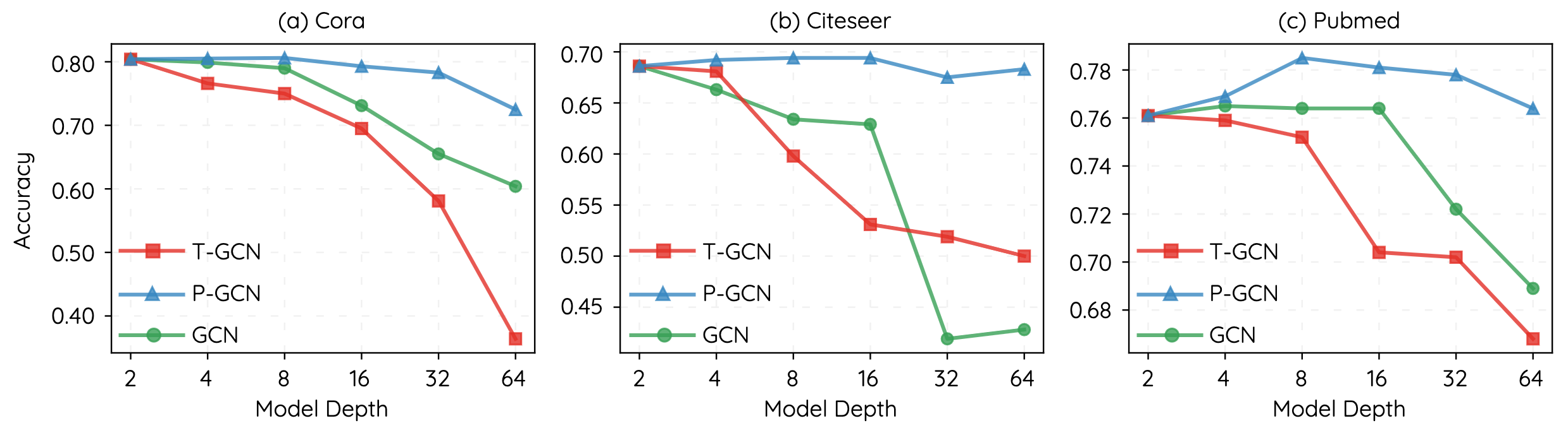
Figure 1. Performance degradation of GCNs, P-GCNs and T-GCNs. A T-GCN performs only TRANs in hidden layers, while a P-GCN performs only PROPs in hidden layers. Due to limited space, we only show results on Cora, Citeseer and Pubmed.

To investigate the role of TRANs in performance degradation, we need to exclude the influence of PROPs. To this end, we disentangle the two operations and build two variants of GCNs: 1) T-GCNs that only perform TRAN in each hidden layer; 2) P-GCNs that only perform PROP in each hidden layer.

Formally, denote a GC layer as $\mathrm{GC}(\cdot)$ and a TRAN as $\mathrm{T(\cdot)}$, and let $X\in\mathbb{R}^{n\times d}$ be the input feature matrix. Then, an $L$-layer T-GCN and P-GCN can be represented as

(3) $$H^{(L)} =\mathrm{GC}(\underbrace{\mathrm{T}\circ\cdots\circ\mathrm{T}}_{L-2}(\mathrm{GC}(X)))\quad\text{(T-GCN)},$$

$$H^{(L)} =\mathrm{GC}(\hat{A}^{L-2}\mathrm{GC}(X))\quad\text{(P-GCN)}.$$

Note the parameters of the two models in different layers are not shared.

We train three models, i.e., vanilla GCN, P-GCN and T-GCN, of different depths on three benchmark datasets: Cora, Citeseer and Pubmed (Sen et al., 2008), and plot test accuracy in Fig. 1. Here the model depth varies from 2 to 64. It can be seen that T-GCN suffers even more severe performance degradation than GCNs. E.g., on Cora, the accuracy drops to 0.4 for 64-layer T-GCN, compared with the accuracy of 0.6 of 64-layer vanilla GCN; by contrast, although the performance of P-GCNs also drops when the the model goes very deep (e.g. 64 layers), the accuracy only drops to 0.72. Such observations deviate from the conventional belief (Li et al., 2018; Chen et al., 2019) that more PROPs will hurt the model performance more severely. Instead, we find that stacking more TRANs introduces larger performance drop and TRANs contribute more than PROPs in this study.

3.3. Transformation operations cause variance inflammation

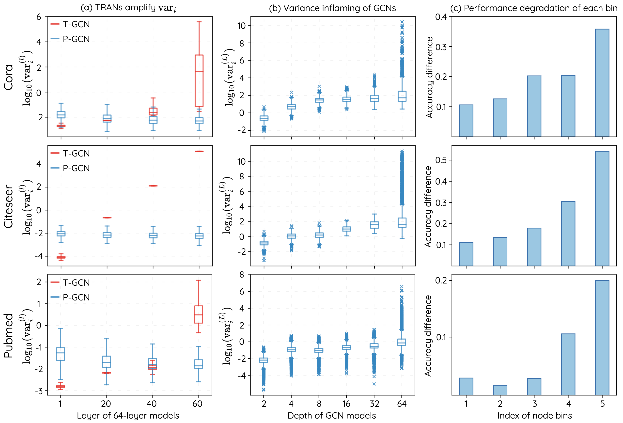
Figure 2. (a) Node-wise feature variance, i.e., $\mathrm{var}_{i}^{(l)}$ of all nodes in different layers ($l=1,20,40,60$) of 64-layer T-GCN and P-GCN models. Results are shown in log scale with a base of 10. Note that the two models are both 64-layer models. Outlier points are not shown for better comparison of the two models. (b) Node-wise feature variance of representations of the last layer, i.e., $\mathrm{var}_{i}^{(L)}$ (in log scale with a base of 10) for $L=2,4,68,16,32,64$ of all nodes. Note that models in this sub-figure are GCNs of different model depths. (c) Performance difference between a 2-layer and a 64-layer model for each node bin. From $S_{1}$ to $S_{5}$, $\mathrm{var}_{i}^{(L)}$ increases. Due to limited space, we only show results on Core, Citeseer and Pubmed.

We then investigate why stacking more TRANs would hurt the performance of deep models. We experimentally examine their effects on node representations, and find that TRANs tend to amplify the node-wise feature variance. As a result, as a GCN model becomes deeper, it contains more TRANs and hence its output node-wise feature variance becomes increasingly large in general. We refer to this phenomenon as variance inflammation. Here the node-wise feature variance refers to the variance of each node’s features. Formally, the feature variance of node $i$ in the $l$-th layer is

(4) $$\mathrm{var}_{i}^{(l)} =\frac{1}{d_{l}}\sum_{j=1}^{d_{l}}\left(h_{ij}^{(l)}-\mu_{i}^{(l)}\right)^{2},$$

where $h_{ij}$ is the the $j$-th feature of node $i$, $\mu_{i}^{(l)}=\frac{1}{d_{l}}\sum_{j=1}^{d_{l}}h_{ij}^{(l)}$ is the mean of the features, and $d_{l}$ denotes the feature dimension.

We plot how $\mathrm{var}_{i}^{(l)}$ changes with the layer index $l$ in a 64-layer T-GCN in Fig. 2 (a). Results in 64-layer P-GCN are also included for comparison. As we can see, within a 64-layer T-GCN, the node-wise feature variance in general rises drastically (note that the y-axis is shown in log scale). By contrast, $\mathrm{var}_{i}^{(l)}$ in P-GCN does not show an increasing trend with larger $l$. This observation demonstrates that TRANs tend to amplify node-wise feature variance.

We then plot the node-wise feature variance of the last layer of GCNs with different depths, i.e., $\mathrm{var}_{i}^{(L)}$ with different $L$, in Fig. 2 (b). We can see variance inflammation from the drastic rise in $\mathrm{log(var}_{i}^{(L)})$ from $L=2$ to $L=64$, i.e. such amplification of node feature variance leading to variance inflammation in GCNs.

Moreover, we find that nodes with large feature variance are difficult to classify. We observe this by sorting all the nodes in the graph based on their node-wise feature variance of the last layer, i.e., $\mathrm{var}_{i}^{(64)}$ of a 64-layer GCN, and partitioning the sorted nodes evenly into 5 bins: $S_{1},\cdots,S_{5}$. For each bin, we illustrate the performance degradation by calculating the accuracy difference between this 64-layer model and a 2-layer model. The results are summarized in Fig. 2 (c). We observe that the 64-layer model has relatively larger variance and performs significantly worse than the 2-layer one.

Motivated by these findings, we hypothesize that mitigating variance inflammation, i.e., preventing $\mathrm{var}_{i}$ from being too large, can help mitigate the performance degradation of deep GCNs.

3.4. Techniques to mitigate variance inflammation

To reduce variance inflammation, we propose a technique that scales each node’s feature vector by the $p$-th root of the standard deviation of its features, with $p\geqslant 1$. As the operation is applied in a node-wise manner, we term it Node Normalization ($\mathrm{NodeNorm}$), formally expressed as

(5) $$\mathrm{NodeNorm}({\mathbf{h}_{i}})=\frac{\mathbf{h}_{i}}{(\sigma_{i})^{\frac{1}{p}}},$$

where $\sigma_{i}=\sqrt{\mathrm{var}_{i}}$ is the standard deviation of $\mathbf{h}_{i}$, and $\mathrm{var}_{i}$ is the variance defined in Eqn. (4). Here we omit the layer index $l$ for clarity. In the following part, we use $\mathrm{NodeNorm}_{p}$ to denote $\mathrm{NodeNorm}$ with a specific $p$.

Let $\hat{\mathbf{h}}_{i}\triangleq\mathrm{NodeNorm}({\mathbf{h}_{i}})$ denote the normalized $\mathbf{h}_{i}$, and let $\hat{\mu}_{i}$, $\hat{\sigma}_{i}$ denote the mean and standard deviation of $\hat{\mathbf{h}}_{i}$.

We have

(6) $$\hat{\sigma}_{i} =\sqrt{\frac{1}{d}\sum_{j=1}^{d}\Big{(}\hat{h}_{ij}-\hat{\mu}_{i}\Big{)}^{2}}$$

$$=\sqrt{\frac{1}{d}\sum_{j=1}^{d}\Big{(}\frac{h_{ij}}{\sigma_{i}^{\frac{1}{p}}}-\frac{\mu_{i}}{\sigma_{i}^{\frac{1}{p}}}\Big{)}^{2}}$$

$$=\sigma_{i}^{(1-\frac{1}{p})}.$$

According to Eqn. (6), for large $\sigma_{i}$ ( $\sigma_{i}>1$), $\sigma_{i}^{(1-\frac{1}{p})}\leqslant\sigma_{i}$ if $p\geqslant 1$. Therefore, given $p\geqslant 1$, we have: 1) The $\mathrm{NodeNorm}_{p}$ can reduce the variance of nodes with $\sigma_{i}>1$, and hence alleviating variance inflammation; 2) A smaller $p$ controls variance inflammation more strictly. We can adjust the value of $p$ so that $\mathrm{NodeNorm}$ can collaborate well with GCNs in different scenarios. Specifically, $p=1$ yields the most strict $\mathrm{NodeNorm}$, i.e., $\mathrm{NodeNorm}_{1}$, which normalizes the variance for all nodes to be 1.

Moreover, we note that the existing Layer Normalization (LayerNorm) (Ba et al., 2016) also performs a node-wise variance-scaling operation. We then also investigate whether (and why) LayerNorm is able to address performance degradation in GCNs. Formally, the formulation of LayerNorm is:

(7) $$\mathrm{LayerNorm}({\mathbf{h}_{i}})=\boldsymbol{\alpha}\odot\frac{\mathbf{h}_{i}-\mu_{i}}{\sigma_{i}}+\boldsymbol{\beta},$$

where $\odot$ denotes an element-wise multiplication, and $\boldsymbol{\alpha}$, $\boldsymbol{\beta}$ are learnable parameters. We can see that a LayerNorm consists of three operations: variance-scaling, mean-subtraction, and feature-wise linear transformation ($\boldsymbol{\alpha}$, $\boldsymbol{\beta}$ are the slopes and biases). In particular, the variance-scaling in LayerNorm is essentially our $\mathrm{NodeNorm}_{1}$.

One may argue that LayerNorm does not naturally mitigates variance inflammation, due to the linear transformations. However, we empirically find that LayerNorm operations in deep GCNs are trained to effectively reduce variance inflammation (see Sec. 4.4).

4. Experiments

As observed in existing works (Zhao and Akoglu, 2019; Rong et al., 2020), deep GCNs do not show significant advantage over shallow ones on benchmark settings (e.g., 20-label-per-class setting on Cora). This might be because shallow models are already sufficient to learn good node representations in these settings, as discussed in (Zhao and Akoglu, 2019). Therefore, to demonstrate the benefit of mitigating variance inflammation, we first evaluate $\mathrm{NodeNorm}$ in three exemplar cases where shallow models are insufficient in Sec. 4.1 (i.e., deep models are needed). We then validate whether the proposed $\mathrm{NodeNorm}$ can help alleviating performance degradation of GCNs on benchmark settings in Sec. 4.2. Next, in Sec. 4.3, we apply our proposed $\mathrm{NodeNorm}$ to other GNN architectures to study their effects upon the performance of different GNNs. Finally, we investigate the effectiveness of LayerNorm in alleviating performance degradation.

Table 1. Classification accuracy in cases where deeper models are needed. The first row is result of the original GCNs. Following rows correspond to GCNs with equipped different techniques. The number in parenthesis corresponds to depth of the model that achieves the performance.

	Citation Networks w/ missing features			Citation Networks w/ low label rate			Networks w/ large diameter
	Cora	Citeseer	Pubmed	Cora	Citeseer	Pubmed	USelect-12	USelect-16
GCN	0.7034$\pm$0.0235 (8)	0.4494$\pm$0.0227 (8)	0.4652$\pm$0.0677 (16)	0.6319$\pm$0.0982 (4)	0.5277$\pm$0.0695 (2)	0.6491$\pm$0.0675 (4)	0.8296$\pm$0.0147 (2)	0.8840$\pm$0.0094 (2)
+DropEdge	0.7335$\pm$0.0182 (16)	0.4811$\pm$0.0225 (16)	0.4292$\pm$0.0331 (32)	0.6193$\pm$0.0496 (4)	0.4710$\pm$0.0679 (8)	0.6557$\pm$0.0717 (4)	0.8589$\pm$0.0082 (16)	0.8921$\pm$0.0037 (4)
+PairNorm	0.6947$\pm$0.0230 (64)	0.4475$\pm$0.0201 (32)	0.6683$\pm$0.0387 (32)	0.6168$\pm$0.0624 (16)	0.4924$\pm$0.0503 (8)	0.6445$\pm$0.0663 (32)	0.8665$\pm$0.0113 (32)	0.8983$\pm$0.0098 (32)
+$\mathrm{NodeNorm}_{1}$	0.7207$\pm$0.0122 (64)	0.4861$\pm$0.0224 (32)	0.5751$\pm$0.0504 (16)	0.6420$\pm$0.0301 (16)	0.5516$\pm$0.0702 (16)	0.6813$\pm$0.0350 (64)	0.8677$\pm$0.0099 (32)	0.9017$\pm$0.0063 (32)
+$\mathrm{NodeNorm}_{2}$	0.7361$\pm$0.0180 (16)	0.4957$\pm$0.0199 (32)	0.6106$\pm$0.0387 (16)	0.6605$\pm$0.0420 (16)	0.5551$\pm$0.0685 (4)	0.6908$\pm$0.0432 (32)	0.8700$\pm$0.0138 (32)	0.9028$\pm$0.0128 (32)
+$\mathrm{NodeNorm}_{3}$	0.7395$\pm$0.0312 (16)	0.4683$\pm$0.0311 (8)	0.4713$\pm$0.0626 (32)	0.6580$\pm$0.0544 (8)	0.5618$\pm$0.0715 (4)	0.6694$\pm$0.0619 (8)	0.8697$\pm$0.0138 (32)	0.9026$\pm$0.0093 (32)

4.1. Evaluating effects of proposed $\mathrm{NodeNorm}$ in cases requiring deep models

In this subsection, we evaluate $\mathrm{NodeNorm}$ in three exemplar cases where deep models are needed to learn good node representations.

4.1.1. Experiment settings

We first introduce the exemplar cases:

1. Citation networks with missing features. In (Zhao and Akoglu, 2019), when some input node features are missing in citation graphs, deep models achieve better performance than shallow ones. Here shallow models are not sufficient to learn good node representations because nodes would benefit from a larger neighbourhood to recover effective feature representation.

2. Citation graphs with low label rate. Deeper models achieve better performance than shallow ones on Cora, Citeseer and Pubmed at low training label rate. As explained in (Sun et al., 2019), when training label rate is low, more layers would be needed to reach the supervision information far away.

3. US election datasets. USelect-12 and USelect-16 datasets (Jia and Benson, 2020) are geographical graphs induced from statistics of United States (US) election of year 2012 and year 2016. Nodes represent US counties, and edges connect nodes whose corresponding counties are geographically bordering. Node features are demographic statistics such as income, education, population. The graph structures of the two datasets are exactly the same. Deep model significantly outperform shallow ones on them, possibly because their graph has a diameter of 69, which is notably larger than that of the commonly used datasets (e.g. about 20). In addition, the average shortest path length between node pairs in the two datasets is around 26, over 4 times larger than that of citation networks. Given such a large graph diameter and a long average distance among nodes, deep models would be desired to fully propagate information among nodes and learn good representations.

For the missing-feature case, we follow (Zhao and Akoglu, 2019) to run experiments on Cora, Citeseer and Pubmed with 100% of missing features. We follow widely adopted 20-label-per-class setting (Kipf and Welling, 2016; Zhao and Akoglu, 2019): 20 labeled training nodes per class, 500 validation nodes, 1,000 test nodes. For the case of low label rate citation graphs, we run experiments on Cora, Citeseer and Pubmed with the 2-label-per-class setting (label rates for three datasets are 0.52%, 0.36%, and 0.03%). The sizes of validation and test sets are 500 and 1,000, as in the commonly adopted 20-label-per-class setting. For the US election datasets, we randomly split the nodes into train/val/test by 60%/20%/20% (Jia and Benson, 2020), and follow (Huang et al., 2020) to conduct a binary node classification task.

For baseline methods, we choose PairNorm (Zhao and Akoglu, 2019) and DropEdge (Rong et al., 2020), which are the best performing generic (i.e., plug-in) methods to address performance degradation of GCNs and other GNN architectures. For DropEdge, results are obtained with the PyTorch Geometric library (Fey and Lenssen, 2019) implementation of DropEdge; for PairNorm, results are obtained using their official implementation. Here we do not compare works designing new GNN architectures that suffer little performance degradation (Li et al., 2020; Chen et al., 2020), since they are orthogonal to our design. Instead, we discuss these methods in Sec. 4.3.

We run experiments with GCNs of {2,4,8,16,32,64} layers. To make the results more reliable, we run each experiment with 10 different random splits of the dataset and report the mean and standard deviation, as suggested by (Shchur et al., 2018). We add residual connections (He et al., 2016; Li et al., 2018) in each layer to avoid training difficulty caused by gradient vanishing. We use 64 hidden dimension for all methods. For $\mathrm{NodeNorm}$, we run experiments with $p=1,2,3$.

4.1.2. Results

Tab. 1 summarizes the best average accuracy and corresponding model depth of the experiments above. In general, with the help of $\mathrm{NodeNorm}$, deeper models achieve much better performance than shallow ones. Specifically, the best performance of $\mathrm{NodeNorm}$-augmented GCNs is achieved by deep models (e.g. 64-layer), and is higher than the best performance of vanilla GCNs, which is generally obtained by shallow models (e.g. 2-layer).

Though both vanilla GCNs and $\mathrm{NodeNorm}$-augmented GCNs are capable of aggregating information from distant nodes when their model depth increases (Gilmer et al., 2017; Hamilton et al., 2017), vanilla GCNs do not perform better as they become deeper. This is because variance inflammation (along with other factors like oversmoothing) offsets the benefit of aggregating distant node information and even leads to performance degradation. By contrast, deep GCNs augmented with $\mathrm{NodeNorm}$ successfully outperform their shallow counterparts because $\mathrm{NodeNorm}$ resolves variance inflammation.

Tab. 1 also show that the baseline methods, i.e., DropEdge and PairNorm, are able to alleviate performance degradation of deep models to some extent, but they are inferior to our proposed variance $\mathrm{NodeNorm}$.

Among $\mathrm{NodeNorm}$ with different $p$, $\mathrm{NodeNorm}_{2}$ has the best performance in 5 out of 8 scenarios. $\mathrm{NodeNorm}_{3}$ also stands out in two cases. In addition, $\mathrm{NodeNorm}_{1}$ is also among the top-3 best-performing techniques in most scenarios. Furthermore, we show in the next section that $\mathrm{NodeNorm}_{1}$ is the most effective one when the model goes very deep (e.g., 64-layers).

Another interesting observation is that, with varying $p$, the optimal model depth can be different. In general, smaller $p$ corresponds to a larger optimal model depth. One possible explanation is that shallower models suffer less variance inflammation, thus requiring less strict variance controlling to achieve better performance.

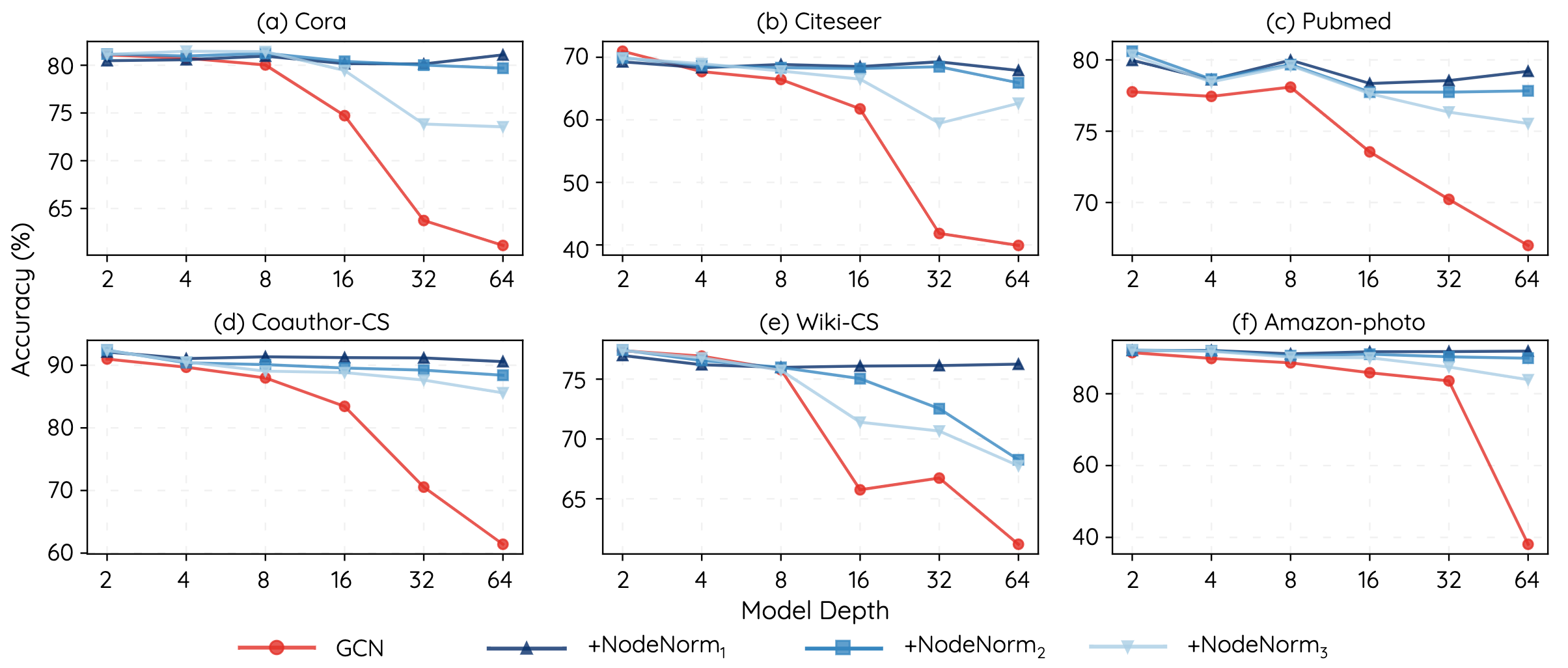
Figure 3. Classification accuracy w.r.t. model depth. It can be seen all variance-controlling techniques are able to mitigate performance degradation. Our $\mathrm{NodeNorm}_{1}$ enables deep models to compete with shallow ones by strictly controlling node-wise variance, i.e., ensuring all $\mathrm{var}_{i}$ to be 1

4.2. Evaluating effects of proposed $\mathrm{NodeNorm}$ on benchmark datasets

To further investigate whether $\mathrm{NodeNorm}$ can help resolve performance degradation of deep GCNs, we evaluate the proposed $\mathrm{NodeNorm}$ on 6 commonly used benchmark datasets.

We first run experiments on 6 node classification datasets of various graph types: three benchmark citation datasets (Sen et al., 2008) Cora, Citeseer and Pubmed, a co-authorship dataset Coauthor-CS (Shchur et al., 2018), a web-page dataset Wiki-CS (Mernyei and Cangea, 2020), and a product co-purchasing dataset Amazon-photo (Shchur et al., 2018). For the three citation networks Cora, Citeseer and Pubmed, we follow the widely adopted 20-label-per-class setting (Kipf and Welling, 2016; Veličković et al., 2017; Xu et al., 2018; Chen et al., 2019). For Coauthor-CS, we also run experiments with 10 splits that are randomly generated based on splitting rules in (Verma et al., 2019). For Wiki-CS, we use the 20 splits provided in (Mernyei and Cangea, 2020). For Amazon-photo, following (Shchur et al., 2018) we adopt the same split setting as the three citation networks. The evaluation metric for these datasets is classification accuracy. We run experiment with GCNs with {2, 4, 8, 16, 32, 64} layers and use $p=1,2,3$ for $\mathrm{NodeNorm}_{p}$.

Table 2. Classification accuracy of $\mathrm{NodeNorm}_{1}$, PairNorm and Dropedge on a widely used split of Cora, Citeseer and Pubmed.

Dataset	Method	Model depth
		2	32	64
Cora	$\mathrm{NodeNorm}_{1}$	0.830	0.829	0.837
	PairNorm	0.783	0.759	0.778
	DropEdge	0.828	0.811	0.789
Citeseer	$\mathrm{NodeNorm}_{1}$	0.729	0.724	0.731
	PairNorm	0.648	0.615	0.614
	DropEdge	0.723	0.700	0.651
Pubmed	$\mathrm{NodeNorm}_{1}$	0.807	0.808	0.804
	PairNorm	0.756	0.768	0.737
	DropEdge	0.796	0.782	0.769

As shown in Fig. 3, compared with vanilla GCNs, models with $\mathrm{NodeNorm}$ suffer much less accuracy drop when they get deep. In particular, $\mathrm{NodeNorm}_{1}$ enables very deep models (e.g., 64-layer) to achieve comparable performance with shallow ones (e.g., 2-layer). The results well demonstrate that mitigating variance inflammation indeed helps address performance degradation.

This is further justified by comparing $\mathrm{NodeNorm}_{p}$ with varying $p$. For deep models (e.g. 64-layers) that suffer severe variance inflammation, the model performance increases as $p$ decreases from 3 to 1. The comparison shows that techniques that control variance inflammation more strictly (with a smaller $p$) can address performance degradation more effectively for very deep models.

Furthermore, we compare our $\mathrm{NodeNorm}_{1}$, the most effective $\mathrm{NodeNorm}$ for very deep models, with the baseline DropEdge (Rong et al., 2020) and PairNorm (Zhao and Akoglu, 2019) methods on benchmark datasets. For fair comparison, we follow (Rong et al., 2020; Zhao and Akoglu, 2019) to run experiments on Cora, Citeseer and Pubmed in the 20-label-per-class semi-supervised classification setting, with a widely used standard split (Kipf and Welling, 2016; Veličković et al., 2017). Results for DropEdge are from their GitHub repository. For PairNorm, 2-layer results are reported in their paper, and we reproduce other results using their reported settings.

Tab 2 summarizes the results. We can see though Dropedge and PairNorm alleviate performance degradation to some extent, deep models with these methods still underperform their shallow counterparts. In comparison, our $\mathrm{NodeNorm}_{1}$ successfully addresses the performance degradation, enabling GCNs of 32 or 64 layers to achieve comparable results with 2-layer GCNs.

Note that in the above results, deep GCNs do not show significant advantage over shallow ones. It is because in benchmark settings, shallow models might be sufficient to learn good representations (discussed in (Zhao and Akoglu, 2019)). Nevertheless, our $\mathrm{NodeNorm}$ successfully enables deep models to match the performance of shallow ones.

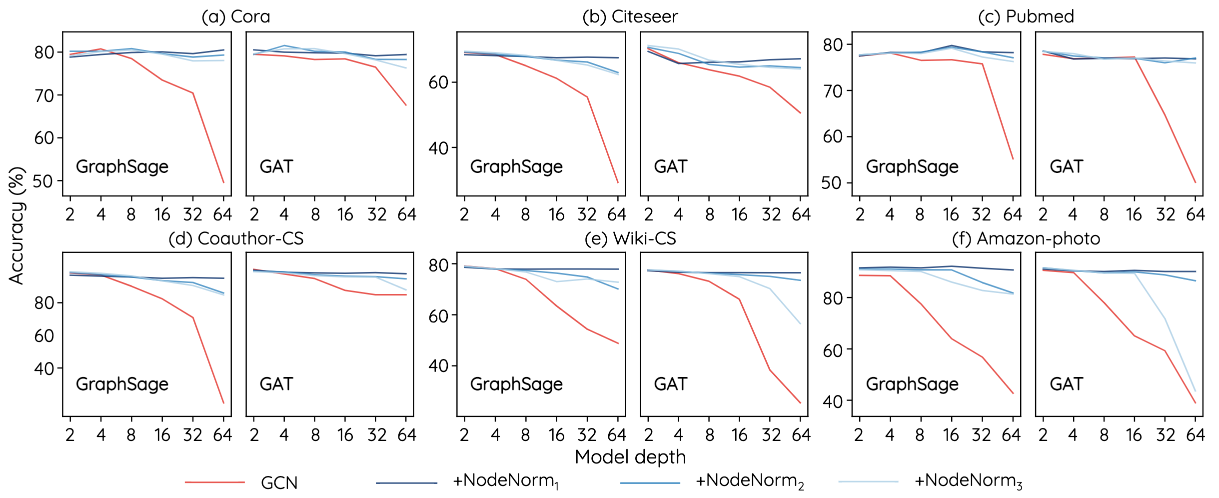
Figure 4. Classification accuracy w.r.t. model depth of GAT and GraphSage.

4.3. Applying variance-controlling to other GNN architectures

Table 3. Best AUC-ROC and corresponding model depth on Obgn-proteins of GENs with and without $\mathrm{NodeNorm}_{1}$.

Method	AUC-ROC
GEN	0.7936$\pm$0.0086 (64)
+$\mathrm{NodeNorm}_{1}$	0.8226$\pm$0.0093 (64)

We apply $\mathrm{NodeNorm}$ to other GNN architectures to study whether variance-controlling can further improve their performance. Below we first experiment on GNNs that also suffer performance degradation when the model gets deep (Hamilton et al., 2017; Veličković et al., 2017), and then on those that can go deep without performance drop (Chen et al., 2020; Li et al., 2020).

We first apply the variance-controlling techniques (i.e. $\mathrm{NodeNorm}$) to other popular GNN architectures that also suffer from performance degradation, including GAT (Veličković et al., 2017) and GraphSage (Hamilton et al., 2017), which achieve high performance in the node classification task. We conduct experiments using the same setting as in Sec. 4.2. As shown in Fig. 4, the variance-controlling techniques generalize well to these architectures, mitigating their performance degradation effectively. In particular, $\mathrm{NodeNorm}$ enables deep GAT or GraphSage models to compete with their shallow counterparts. The results well demonstrate that controlling variance also addresses performance degradation for other GNN architectures in addition to GCNs.

Table 4. Best accuracy and corresponding model depth on web-pages datasets of GCNIIs with and without $\mathrm{NodeNorm}_{1}$.

Method	Dataset
	Cornell	Texas	Wisconsin
GCNII	0.7496$\pm$0.0514 (16)	0.6946$\pm$0.0793 (32)	0.7412$\pm$0.0526 (16)
+$\mathrm{NodeNorm}_{1}$	0.8054$\pm$0.0692 (16)	0.7892$\pm$0.0637 (32)	0.8314$\pm$0.0542 (16)

There are also works obtaining deep GNNs by designing new GNN architectures that can naturally go deep without suffering severe performance degradation, which are orthogonal to our design in this work. We also include them in experiments to further show the effectiveness of our proposed variance controlling techniques. In particular, we apply $\mathrm{NodeNorm}$ to GEN (Li et al., 2020) and GCNII (Chen et al., 2020), which are among the best new GNN architectures that do not suffer declined performance as the model grows deep. We run experiments with the two models of {2, 4, 8, 16, 32, 64} layers. For GEN, we follow (Li et al., 2020) to run experiments on Ogbn-proteins (Hu et al., 2020), each with 5 random seeds, since the dataset split in (Hu et al., 2020) is practically meaningful and random split may not make sense anymore. We use the PyTorch Geometric library (Fey and Lenssen, 2019) implementation of GENs, which is provided by (Li et al., 2020). For GCNII, we follow (Chen et al., 2020) to conduct experiments on web-page networks (Pei et al., 2020): Cornell, Texas and Wisconsin, where each experiment is run with 10 different dataset splits. In the web-page networks, nodes and edges represent web pages and hyperlinks respectively. We use their released code for implementation. For both architectures, we follow experiment settings in their GitHub repositories. We do not tune hyperparameters or use training tricks like one-hot-node-encoding in (Li et al., 2020). We take $\mathrm{NodeNorm}_{1}$ as an example of $\mathrm{NodeNorm}$ as it is simple yet effective in addressing performance degradation for very deep models.

As shown in Tab. 3 and Tab. 4, our proposed $\mathrm{NodeNorm}_{1}$ improve the performance of GEN and GCNII. Notably, $\mathrm{NodeNorm}_{1}$ improves the performance of GCNII by a margin of 10% on Texas and Wisconsin datasets. We emphasize again that GEN and GCNII are orthogonal to our work—we focus on understanding and addressing performance degradation of GCNs (and other popular GNNs), and claim that reducing variance inflammation helps mitigate this issue, while their contributions are the proposed architectures, i.e., GEN or GCNII.

4.4. Investigating the effectiveness of $\mathrm{LayerNorm}$

As mentioned in Sec. 3.4, LayerNorm (Ba et al., 2016) also performs a variance-scaling operation. Inspired by this, we investigate whether and why LayerNorm also helps address performance degradation in GCNs.

We experiment with LayerNorm in the three exemplar cases where deep GCNs are desired (see Sec. 4.1), using the same setting as in Sec. 4.1. As shown in Tab. 5, LayerNorm also helps deeper models to achieve better performance than shallow ones.

Meanwhile, we note that, our proposed $\mathrm{NodeNorm}$ outperform LayerNorm in these experiments: $\mathrm{NodeNorm}_{1}$, $\mathrm{NodeNorm}_{2}$ and $\mathrm{NodeNorm}_{3}$ outperform LayerNorm in 5, 7 and 5 out of 8 settings respectively. This demonstrates that $\mathrm{NodeNorm}$ is more effective than LayerNorm in resolving performance degradation. One possible reason might be that less strict variance controlling is desired in these settings. Therefore, techniques that control node-wise more softly (e.g., $\mathrm{NodeNorm}_{2}$) would outperform those strictly controlling the variance, such as $\mathrm{NodeNorm}_{1}$ and LayerNorm (note that LayerNorm performs the variance-scaling operation that is equivalent to $\mathrm{NodeNorm}_{1}$). Another possible reason is that LayerNorm has learnable parameters $\mathbf{\alpha}$ and $\mathbf{\beta}$ (see Eqn. (7)), which increases the degree of overfitting and hence slightly hurts the performance.

Table 5. Performance comparison of LayerNorm and $\mathrm{NodeNorm}$ in cases where deeper models are needed. The first row shows the results of the original GCNs. Following rows correspond to GCNs with different techniques equipped. The number in parenthesis corresponds to depth of the model that achieves the performance.

	Citation Networks w/ missing features			Citation Networks w/ low label rate			Networks w/ large diameter
	Cora	Citeseer	Pubmed	Cora	Citeseer	Pubmed	USelect-12	USelect-16
GCN	0.7034$\pm$0.0235 (8)	0.4494$\pm$0.0227 (8)	0.4652$\pm$0.0677 (16)	0.6319$\pm$0.0982 (4)	0.5277$\pm$0.0695 (2)	0.6491$\pm$0.0675 (4)	0.8296$\pm$0.0147 (2)	0.8840$\pm$0.0094 (2)
+LayerNorm	0.7160$\pm$0.0199 (64)	0.4860$\pm$0.0180 (32)	0.5450$\pm$0.0577 (4)	0.6348$\pm$0.0385 (16)	0.5569$\pm$0.0747 (16)	0.6820$\pm$0.0464 (32)	0.8657$\pm$0.0104 (32)	0.8983$\pm$0.0113 (32)
+$\mathrm{NodeNorm}_{1}$	0.7207$\pm$0.0122 (64)	0.4861$\pm$0.0224 (32)	0.5751$\pm$0.0504 (16)	0.6420$\pm$0.0301 (16)	0.5516$\pm$0.0702 (16)	0.6813$\pm$0.0350 (64)	0.8677$\pm$0.0099 (32)	0.9017$\pm$0.0063 (32)
+$\mathrm{NodeNorm}_{2}$	0.7361$\pm$0.0180 (16)	0.4957$\pm$0.0199 (32)	0.6106$\pm$0.0387 (16)	0.6605$\pm$0.0420 (16)	0.5551$\pm$0.0685 (4)	0.6908$\pm$0.0432 (32)	0.8700$\pm$0.0138 (32)	0.9028$\pm$0.0128 (32)
+$\mathrm{NodeNorm}_{3}$	0.7395$\pm$0.0312 (16)	0.4683$\pm$0.0311 (8)	0.4713$\pm$0.0626 (32)	0.6580$\pm$0.0544 (8)	0.5618$\pm$0.0715 (4)	0.6694$\pm$0.0619 (8)	0.8697$\pm$0.0138 (32)	0.9026$\pm$0.0093 (32)

However, since LayerNorm performs three operations: variance-scaling, mean-subtraction and linear transformation (see Eqn. (7)), more investigation is needed to demonstrate that variance-scaling is the key to the effectiveness of LayerNorm in resolving performance degradation of deep GCNs. We then ablatively study the effects of the three operations on addressing performance degradation. Specifically, we study two variants of LayerNorm:

(8) $$\mathrm{LayerNorm}^{*}({\mathbf{h}_{i}})=\frac{\mathbf{h}_{i}-\mu_{i}}{\sigma_{i}},$$

(9) $$\mathrm{LayerNorm\text{-}MS}({\mathbf{h}_{i}})=\mathbf{h}_{i}-\mu_{i}.$$

LayerNorm* does not include linear transformations, while the LayerNorm-MS variant performs only Mean-Subtraction (MS).

We conduct experiments with the two variants of 64 layers, with the same settings as in Sec. 4.2, and show results in Fig. 5. We can see that GCNs with LayerNorm*, LayerNorm or $\mathrm{NodeNorm}_{1}$ perform comparatively, while those with LayerNorm-MS perform significantly worse (on 4 datasets even worse than baseline GCNs). Note that $\mathrm{NodeNorm}_{1}$ is equivalent to the variance-scaling step in LayerNorm. The above observations show that linear transformation and the mean-subtraction step are not critical for improving deep GCNs performance; instead, variance-scaling is the step that really works. This demonstrates that reducing variance inflammation is the key to addressing performance degradation.

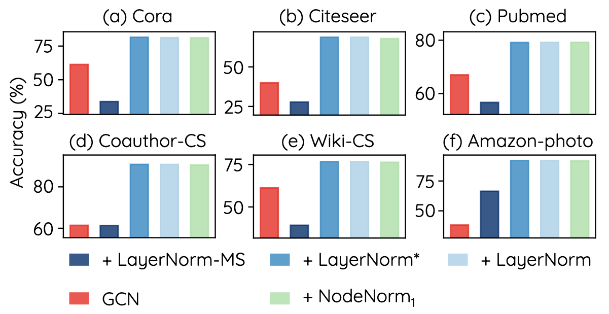
Figure 5. Classification accuracy of 64-layer GCNs with LayerNorm-MS and LayerNorm*. We also include results of the baseline GCNs, GCNs with $\mathrm{NodeNorm}_{1}$ or LayerNorm for clearer comparison.

5. Conclusion

In this paper, we investigate the performance degradation problem of GCNs by focusing on effects of TRANsformation operations (TRANs). We find TRANs contribute significantly to the declined performance, providing a new understanding for the community. Furthermore, we find TRANs tend to amplify the node-wise feature variance of node representations, and then as GCNs get deeper, its node-wise feature variance becomes increasingly larger. We also find deep GCNs perform significantly worse than shallow ones on nodes with relatively large feature variance. We thus hypothesize and experimentally justify that mitigating variance inflammation effectively addresses performance degradation of GCNs. In particular, a simple variance-controlling technique termed $\mathrm{NodeNorm}$, which normalizes each node’s hidden features with its own standard deviation, is developed. We experimentally prove it can enable deep GCNs (e.g. 64-layer) to compete with and even outperform shallow ones (e.g. 2-layer). $\mathrm{NodeNorm}$ outperforms existing best methods on addressing performance degradation of GCNs, and can generalize to other GNN architectures.

References

- (1)
- Ba et al. (2016) Jimmy Lei Ba, Jamie Ryan Kiros, and Geoffrey E Hinton. 2016. Layer normalization. arXiv preprint arXiv:1607.06450 (2016).
- Chen et al. (2019) Deli Chen, Yankai Lin, Wei Li, Peng Li, Jie Zhou, and Xu Sun. 2019. Measuring and Relieving the Over-smoothing Problem for Graph Neural Networks from the Topological View. arXiv preprint arXiv:1909.03211 (2019).
- Chen et al. (2020) Ming Chen, Zhewei Wei, Zengfeng Huang, Bolin Ding, and Yaliang Li. 2020. Simple and Deep Graph Convolutional Networks. arXiv preprint arXiv:2007.02133 (2020).
- Defferrard et al. (2016) Michaël Defferrard, Xavier Bresson, and Pierre Vandergheynst. 2016. Convolutional neural networks on graphs with fast localized spectral filtering. In Advances in neural information processing systems. 3844–3852.
- Fey and Lenssen (2019) Matthias Fey and Jan E. Lenssen. 2019. Fast Graph Representation Learning with PyTorch Geometric. In ICLR Workshop on Representation Learning on Graphs and Manifolds.
- Gilmer et al. (2017) Justin Gilmer, Samuel S Schoenholz, Patrick F Riley, Oriol Vinyals, and George E Dahl. 2017. Neural message passing for quantum chemistry. In Proceedings of the 34th International Conference on Machine Learning-Volume 70. JMLR. org, 1263–1272.
- Hamilton et al. (2017) Will Hamilton, Zhitao Ying, and Jure Leskovec. 2017. Inductive representation learning on large graphs. In Advances in neural information processing systems. 1024–1034.
- He et al. (2016) Kaiming He, Xiangyu Zhang, Shaoqing Ren, and Jian Sun. 2016. Deep residual learning for image recognition. In Proceedings of the IEEE conference on computer vision and pattern recognition. 770–778.
- Hu et al. (2020) Weihua Hu, Matthias Fey, Marinka Zitnik, Yuxiao Dong, Hongyu Ren, Bowen Liu, Michele Catasta, and Jure Leskovec. 2020. Open graph benchmark: Datasets for machine learning on graphs. arXiv preprint arXiv:2005.00687 (2020).
- Huang et al. (2020) Qian Huang, Horace He, Abhay Singh, Ser-Nam Lim, and Austin R Benson. 2020. Combining Label Propagation and Simple Models Out-performs Graph Neural Networks. arXiv preprint arXiv:2010.13993 (2020).
- Ioffe and Szegedy (2015) Sergey Ioffe and Christian Szegedy. 2015. Batch normalization: Accelerating deep network training by reducing internal covariate shift. arXiv preprint arXiv:1502.03167 (2015).
- Jia and Benson (2020) Junteng Jia and Austion R Benson. 2020. Residual Correlation in Graph Neural Network Regression. In Proceedings of the 26th ACM SIGKDD International Conference on Knowledge Discovery & Data Mining. 588–598.
- Kipf and Welling (2016) Thomas N Kipf and Max Welling. 2016. Semi-supervised classification with graph convolutional networks. arXiv preprint arXiv:1609.02907 (2016).
- Klambauer et al. (2017) Günter Klambauer, Thomas Unterthiner, Andreas Mayr, and Sepp Hochreiter. 2017. Self-normalizing neural networks. In Advances in neural information processing systems. 971–980.
- Klicpera et al. (2018) Johannes Klicpera, Aleksandar Bojchevski, and Stephan Günnemann. 2018. Predict then propagate: Graph neural networks meet personalized pagerank. arXiv preprint arXiv:1810.05997 (2018).
- Li et al. (2019) Guohao Li, Matthias Muller, Ali Thabet, and Bernard Ghanem. 2019. Deepgcns: Can gcns go as deep as cnns?. In Proceedings of the IEEE International Conference on Computer Vision. 9267–9276.
- Li et al. (2020) Guohao Li, Chenxin Xiong, Ali Thabet, and Bernard Ghanem. 2020. Deepergcn: All you need to train deeper gcns. arXiv preprint arXiv:2006.07739 (2020).
- Li et al. (2018) Qimai Li, Zhichao Han, and Xiao-Ming Wu. 2018. Deeper insights into graph convolutional networks for semi-supervised learning. In Thirty-Second AAAI Conference on Artificial Intelligence.
- Mernyei and Cangea (2020) Péter Mernyei and Cătălina Cangea. 2020. Wiki-CS: A Wikipedia-Based Benchmark for Graph Neural Networks. arXiv preprint arXiv:2007.02901 (2020).
- Nair and Hinton (2010) Vinod Nair and Geoffrey E Hinton. 2010. Rectified linear units improve restricted boltzmann machines. In ICML.
- Oono and Suzuki (2019) Kenta Oono and Taiji Suzuki. 2019. On asymptotic behaviors of graph cnns from dynamical systems perspective. arXiv preprint arXiv:1905.10947 (2019).
- Pei et al. (2020) Hongbin Pei, Bingzhe Wei, Kevin Chen-Chuan Chang, Yu Lei, and Bo Yang. 2020. Geom-GCN: Geometric Graph Convolutional Networks. In International Conference on Learning Representations. https://openreview.net/forum?id=S1e2agrFvS
- Rong et al. (2020) Yu Rong, Wenbing Huang, Tingyang Xu, and Junzhou Huang. 2020. DropEdge: Towards Deep Graph Convolutional Networks on Node Classification. In International Conference on Learning Representations. https://openreview.net/forum?id=Hkx1qkrKPr
- Sen et al. (2008) Prithviraj Sen, Galileo Namata, Mustafa Bilgic, Lise Getoor, Brian Galligher, and Tina Eliassi-Rad. 2008. Collective classification in network data. AI magazine 29, 3 (2008), 93–93.
- Shchur et al. (2018) Oleksandr Shchur, Maximilian Mumme, Aleksandar Bojchevski, and Stephan Günnemann. 2018. Pitfalls of graph neural network evaluation. arXiv preprint arXiv:1811.05868 (2018).
- Sun et al. (2019) Ke Sun, Zhanxing Zhu, and Zhouchen Lin. 2019. Multi-stage self-supervised learning for graph convolutional networks. arXiv preprint arXiv:1902.11038 (2019).
- Telgarsky (2016) Matus Telgarsky. 2016. Benefits of depth in neural networks. arXiv preprint arXiv:1602.04485 (2016).
- Vaswani et al. (2017) Ashish Vaswani, Noam Shazeer, Niki Parmar, Jakob Uszkoreit, Llion Jones, Aidan N Gomez, Łukasz Kaiser, and Illia Polosukhin. 2017. Attention is all you need. In Advances in neural information processing systems. 5998–6008.
- Veličković et al. (2017) Petar Veličković, Guillem Cucurull, Arantxa Casanova, Adriana Romero, Pietro Lio, and Yoshua Bengio. 2017. Graph attention networks. arXiv preprint arXiv:1710.10903 (2017).
- Verma et al. (2019) Vikas Verma, Meng Qu, Alex Lamb, Yoshua Bengio, Juho Kannala, and Jian Tang. 2019. GraphMix: Regularized Training of Graph Neural Networks for Semi-Supervised Learning. arXiv preprint arXiv:1909.11715 (2019).
- Wu et al. (2019) Felix Wu, Tianyi Zhang, Amauri Holanda de Souza Jr, Christopher Fifty, Tao Yu, and Kilian Q Weinberger. 2019. Simplifying graph convolutional networks. arXiv preprint arXiv:1902.07153 (2019).
- Xu et al. (2018) Keyulu Xu, Chengtao Li, Yonglong Tian, Tomohiro Sonobe, Ken-ichi Kawarabayashi, and Stefanie Jegelka. 2018. Representation learning on graphs with jumping knowledge networks. arXiv preprint arXiv:1806.03536 (2018).
- Zhao and Akoglu (2019) Lingxiao Zhao and Leman Akoglu. 2019. PairNorm: Tackling Oversmoothing in GNNs. arXiv preprint arXiv:1909.12223 (2019).
- Zhou et al. (2018) Jie Zhou, Ganqu Cui, Zhengyan Zhang, Cheng Yang, Zhiyuan Liu, Lifeng Wang, Changcheng Li, and Maosong Sun. 2018. Graph neural networks: A review of methods and applications. arXiv preprint arXiv:1812.08434 (2018).