Seemingly Unrelated Regression with Measurement Error: Estimation via Markov chain Monte Carlo and Mean Field Variational Bayes Approximation

Abstract

Linear regression with measurement error in the covariates is a heavily studied topic, however, the statistics/econometrics literature is almost silent to estimating a multi-equation model with measurement error. This paper considers a seemingly unrelated regression model with measurement error in the covariates and introduces two novel estimation methods: a pure Bayesian algorithm (based on Markov chain Monte Carlo techniques) and its mean field variational Bayes (MFVB) approximation. The MFVB method has the added advantage of being computationally fast and can handle big data. An issue pertinent to measurement error models is parameter identification, and this is resolved by employing a prior distribution on the measurement error variance. The methods are shown to perform well in multiple simulation studies, where we analyze the impact on posterior estimates arising due to different values of reliability ratio or variance of the true unobserved quantity used in the data generating process. The paper further implements the proposed algorithms in an application drawn from the health literature and shows that modeling measurement error in the data can improve model fitting.

1 Introduction

The seemingly unrelated regression (SUR) model consists of a system of linear multiple regression equations such that each equation has a different continuous dependent variable with a potentially different set of exogenous explanatory variables (covariates) and the errors are correlated across equations (Zellner, 1962). When the conditions of the SUR model apply, estimators obtained from SUR are more efficient relative to ordinary least squares estimators. The optimality feature and other theoretical properties of the SUR estimator within the frequentist framework are well studied in Srivastava and Dwivedi (1979), Srivastava and Giles (1987) and Fiebig (2001). The Bayesian approach to estimating SUR model was introduced in Zellner (1971), where the author analytically derived the conditional posterior densities of the parameters. Given the conditional posteriors, the model can then be estimated using a Markov chain Monte Carlo (MCMC) technique, known as Gibbs sampling (Geman and Geman, 1984; Casella and George, 1992). Since the introduction in Zellner (1971), the literature on Bayesian analysis of SUR has grown considerably in various directions, including estimation via MCMC (Percy, 1992; Griffiths and Chotikapanich, 1997; Griffiths and Valenzuela, 2006) and direct Monte Carlo approach (Zellner and Ando, 2010; Ando and Zellner, 2010), prediction in SUR model (Percy, 1992) and several model extensions that include restricted SUR (Steel, 1992), SUR with serially correlated errors and time varying parameters (Chib and Greenberg, 1995) and semiparametric inference in SUR model (Koop et al., 2005).

The existing literature on SUR models including the quoted articles have worked based on the assumption that the covariates are measured correctly. Nonetheless, in practice there can emerge situations where one or more of the covariates are recorded with error, thus giving rise to SUR with measurement error (hereafter SURME). Modeling measurement error within a SUR structure or more generally in a multi-equation system has largely gone unnoticed in the literature (both frequentist and Bayesian), the only exception is Carroll et al. (2006a, b) explained in the next paragraph. In contrast, there has been considerable work on single equation models with measurement error. Within a linear regression framework, it is well known that measurement error in the data leads to bias and inconsistency in ordinary least squares (OLS) estimator (see for instance Cheng and Van Ness (1999), Fuller (1987), Wansbeek and Meijer (2000), Rao et al. (2008) and Hu and Wansbeek (2017)). To achieve consistency of OLS estimator, side assumptions are required such as known measurement error variance or known reliability ratio. However, consistent estimator of regression parameters without the side assumptions can be constructed when measurement errors have replicated observations (Shalabh, 2003). Measurement error in nonlinear models is discussed in Carroll et al. (2006b) along with the Bayesian analysis of linear and non-linear measurement error models.

Within the multi-equation framework, Carroll et al. (2006b) consider a combination of linear mixed measurement error model and SUR model to understand the properties of measurement error in food frequency questionnaire data for protein and energy. They adopt the frequentist estimation approach and use a nearby adaptive method based on weighted Akaike information criterion (AIC) to select the best fitting model, a form of model averaging which is popular in the Bayesian literature. Carroll et al. (2006b) find that a fully parameterized model in which measurement errors in the two nutrients are modeled jointly, offers no gain in efficiency compared to fitting each model separately. However, when some parameters are set to zero resulting in a reduced model, considerable gains in efficiency is attained. We may adopt the frequentist approach to estimating SURME model with structural measurement error, but it is fraught with difficulty because the number of parameters become larger than the number of normal equations derived from the likelihood function. In such cases, side assumptions can be used to identify the model as done in linear regression, but even then deriving the maximum likelihood estimators for SURME model is a challenging task. Besides, ignoring measurement error in the data can lead to a poor model fit.

In this paper, we introduce two novel methods—a pure Bayesian algorithm and a mean field variational Bayes (MFVB) technique—to estimate the SURME model where each equation can potentially have a different covariate that is measured with error. Both the approach employs a classical structural form of measurement error and the link between the covariate measured with error and the other covariates (with no measurement error) is modeled through an exposure equation. Identification of parameters is achieved by placing a prior distribution on the measurement error variance. The pure Bayesian approach is analytically simpler and produces tractable conditional distributions which enables the use of Gibbs sampling. However, the MCMC draws of the parameters corresponding to the covariate measured with error tend to be highly correlated. To reduce autocorrelation in MCMC draws, one may consider thinning i.e., use every $l$-th draw in estimating the parameter. Thinning is debatable and while some authors such as Owen (2017) recommend thinning, others such as Link and Eaton (2012) advise against the use of thinning. So, we explore other methods and come up with a more elegant solution to the problem of high autocorrelation i.e., the MFVB approach to estimating SURME model.

We illustrate both the techniques in multiple simulation studies and compare the results to a standard SUR model, where we ignore or do not model the measurement error. In the first set of simulation studies, data are generated from a SURME model using different values of the variance of the true unobserved variable, while holding the reliability ratio fixed. In the second set of simulations, data are generated using different values of reliability ratio, holding the variance of the true unobserved variable at a fixed value. The results suggest that both the proposed methods perform well and correctly highlight the importance of modeling measurement error within the SUR structure when variables are measured with error. In addition, the SURME model is implemented in an application drawn from the health literature and estimated using the two proposed methods. Specifically, weight and high density lipoprotein (HDL) are jointly modeled as a function of several covariates and blood pressure, which is common to both equations and considered to have measurement error. Blood pressure is modeled as a function of the covariates in the exposure equation. Model selection exemplify the practical utility of the SURME model compared to the standard SUR model.

The remainder of the paper is organized as follows. Section 2 presents the SURME model, derives the joint posterior density and proposes a Gibbs sampling algorithm to estimate the model. Section 3 develops the MFVB approximation of the MCMC algorithm. Section 4 demonstrates the two algorithms in several Monte Carlo simulation exercises and Section 5 presents an application drawn from health literature. Section 6 concludes.

2 The SURME Model and Estimation via Gibbs sampling

The seemingly unrelated regression with measurement error (SURME) model incorporates measurement error for covariates in the SUR model and can be expressed in terms of the following equations,

$$y_{mi}=x_{mi}^{\prime}\beta_{m}+z_{mi}\gamma_{m}+\varepsilon_{mi},\qquad m=1,...,M;\;i=1,...,N,$$ (1)

where the response $y_{mi}$ is a scalar, $x_{mi}^{\prime}$ is $\left(1\times k_{m}\right)$ vector of covariates, $z_{mi}$ is a true unobserved scalar covariate that is prone to measurement error, and the subscripts $m$ and $i$ denote the equation number and individual/observation, respectively. Stacking the equations for each $i$, we can write model (1) as follows,

$$y_{i}=X_{i}\beta+Z_{i}\gamma+\varepsilon_{i},\qquad i=1,..,N,$$ (2)

where $y_{i}=\left(y_{1i},...,y_{Mi}\right)^{\prime}$ and $\gamma=\left(\gamma_{1},...,\gamma_{M}\right)^{\prime}$ are vectors of dimension $\left(M\times 1\right)$, and $\beta=\left(\beta_{1},...,\beta_{M}\right)^{\prime}$ is of dimension $(K\times 1)$, where $K=k_{1}+\cdots+k_{M}$. The matrices,

$$X_{i}=\left(\begin{array}[]{ccc}x_{1i}^{\prime}&\cdots&0\\ &\ddots&\\ 0&\cdots&x_{Mi}^{\prime}\end{array}\right)\qquad\mathrm{and}\qquad Z_{i}=\left(\begin{array}[]{cccc}z_{1i}&\cdots&0\\ &\ddots&\\ 0&\cdots&z_{Mi}\end{array}\right),$$

are of dimension $(M\times K)$ and $(M\times M)$, respectively. In addition, the error $\varepsilon_{i}$ is assumed to be independently and identically distributed (i.i.d.) as a normal distribution i.e., $\varepsilon_{i}\sim N(0,\Sigma_{\varepsilon})$ for $i=1,\cdots,N$, where the covariance,

$$\Sigma_{\varepsilon}=\left(\begin{array}[]{ccc}\sigma_{11}&\cdots&\sigma_{1M}\\ \vdots&\ddots&\vdots\\ \sigma_{M1}&\cdots&\sigma_{MM}\end{array}\right),$$

is a symmetric matrix that permits nonzero correlation across equations (or first subscript) for any given individual (or second subscript) and ties each independent regression into a system of equations, hence the phrase seemingly unrelated regression. Measurement error in reference to model (2) arises because $Z_{i}$ is not observed, instead we observe $W_{i}$ which is a sum of the true unobserved quantity $Z_{i}$ and a measurement error term $u_{i}$. This definition implies a classical measurement error (Fuller, 1987). Additionally, we assume that the true unobserved quantity $Z_{i}$ follows a distribution, so that the measurement error model is of the structural form. This can be represented as follows,

$$\widetilde{W}_{i}=\widetilde{Z}_{i}+\widetilde{u}_{i},\qquad\widetilde{u}_{i}\sim N_{M}\left(0,\sigma_{u}^{2}I_{M}\right),\qquad\textit{classical structural form},$$ (3)

where for algebraic simplification, we use the notations $\widetilde{W}_{i}=\left(w_{1i},...,w_{Mi}\right)^{\prime}$, $\widetilde{Z}_{i}=\left(z_{1i},...,z_{Mi}\right)^{\prime}$, $\widetilde{u}_{i}=\left(u_{1i},...,u_{Mi}\right)^{\prime}$, then $W_{i}=diag(\widetilde{W}_{i})$, $Z_{i}=diag(\widetilde{Z}_{i})$, $u_{i}=diag(\widetilde{u}_{i})$ are $\left(M\times M\right)$ diagonal matrices and $I_{M}$ is a ($M\times M$) identity matrix.

An interesting addition to equation (3) is to relate the primary explanatory variable of interest (here $Z_{i}$) to other covariates ($X_{i}$), giving rise to the exposure model. The term “exposure model” comes from epidemiology, where the primary explanatory variable is affected by exposure to “toxicants” or “risk factors”. Therefore, the potential links between the latent variable $Z$ and the other covariates $X$ can be expressed as follows,

$$\widetilde{Z}_{i}=X_{i}\omega+\widetilde{\varepsilon}_{z,i},\qquad\widetilde{\varepsilon}_{z,i}\sim N_{M}\left(0,\sigma_{Z}^{2}I_{M}\right),\qquad\textit{exposure model}.$$ (4)

The three equations (2), (3) and (4) together define our SURME model and the resulting likelihood is derived as follows,

$$\begin{split}&f(y,W,Z|X,\Delta)=\prod_{i=1}^{N}f(y_{i},W_{i},Z_{i}|X,\Delta)\\ &=\prod_{i=1}^{N}\bigg{\{}f(y_{i}|W_{i},Z_{i},X,\Delta)\times f(W_{i}|Z_{i},X,\Delta)\times f(Z_{i}|X,\Delta)\bigg{\}}\\ &=\prod_{i=1}^{N}\bigg{\{}f(y_{i}|Z_{i},X,\Delta)\times f(W_{i}|Z_{i},X,\Delta)\times f(Z_{i}|X,\Delta)\bigg{\}}\\ &=\prod_{i=1}^{N}\bigg{\{}(2\pi)^{-M/2}\,|\Sigma_{\varepsilon}|^{-1/2}\exp\Big{[}-\frac{1}{2}(y_{i}-X_{i}\beta-Z_{i}\gamma)^{\prime}\Sigma_{\varepsilon}^{-1}(y_{i}-X_{i}\beta-Z_{i}\gamma)\Big{]}\\ &\hskip 38.30301pt\times(2\pi)^{-M/2}\,(\sigma_{u}^{2})^{-M/2}\exp\Big{[}-\frac{1}{2\sigma_{u}^{2}}(\widetilde{W}_{i}-\widetilde{Z}_{i})^{\prime}(\widetilde{W}_{i}-\widetilde{Z}_{i})\Big{]}\\ &\hskip 38.30301pt\times(2\pi)^{-M/2}\,(\sigma_{Z}^{2})^{-M/2}\exp\Big{[}-\frac{1}{2\sigma_{Z}^{2}}(\widetilde{Z}_{i}-X_{i}\omega)^{\prime}(\widetilde{Z}_{i}-X_{i}\omega)\Big{]}\bigg{\}},\end{split}$$ (5)

where $\Delta\equiv(\beta,\gamma,\Sigma_{\varepsilon},\omega,\sigma_{Z}^{2},\sigma_{u}^{2})$ and as mentioned earlier, $\widetilde{W}_{i}$ and $\widetilde{Z}_{i}$ are column vectors that contain the diagonal elements of the matrices $W_{i}$ and $Z_{i}$, respectively.

Before proceeding with estimation, we add a few words on identification issues that typically arise with measurement error models. In linear regression with measurement error, identification of parameters require additional assumptions. Such assumptions can be constant measurement error variance, known reliability ratio or some other conditions as presented in Cheng and Van Ness (1999). The same identification conditions are also applicable to the proposed SURME model under the existing distributional assumptions. Nonetheless, we follow a purely Bayesian approach and employ prior distributions to identify the parameters of the model (see Zellner, 1971, Chap. 5).

The Bayesian estimation method combines the likelihood of the model with suitable prior distributions to obtain the joint posterior distribution. We utilize the following prior distributions:

$$\begin{split}&\beta\sim N_{K}\left(\beta_{0},B_{0}\right),\quad\gamma\sim N_{M}\left(\gamma_{0},G_{0}\right),\quad\Sigma_{\varepsilon}^{-1}\sim W_{M}\left(\nu_{0},S_{0}\right),\\ &\omega\sim N_{K}\left(\omega_{0},O_{0}\right),\quad\sigma_{Z}^{2}\sim IG\left(\delta_{1},\delta_{2}\right),\quad\sigma_{u}^{2}\sim IG\left(\delta_{3},\delta_{4}\right),\end{split}$$ (6)

where $W_{M}$ denotes a Wishart distribution of dimension $M$ and $IG$ denotes an inverse gamma distribution. Here we note that if one is not interested in the exposure equation, it can be dropped from the model. In such a case, $\tilde{Z}_{i}\sim N(\mu,\sigma_{Z}^{2}I_{M})$ and $\mu$ can be given a normal prior as $\mu\sim N(\mu_{0},\sigma_{\mu}^{2}I_{M})$. Coming back to the SURME model, the joint posterior distribution can be obtained by combining the likelihood (5) with the prior distributions (6) as follows,

$$\begin{split}p\left(\Delta,Z|y,X,W\right)&\propto\prod_{i=1}^{N}\Bigg{\{}\left|\Sigma_{\varepsilon}\right|^{-1/2}\exp\left[-\frac{1}{2}\left(y_{i}-X_{i}\beta-Z_{i}\gamma\right)^{\prime}\Sigma_{\varepsilon}^{-1}\left(y_{i}-X_{i}\beta-Z_{i}\gamma\right)\right]\\ &\quad\times\left(\sigma_{u}^{2}\right)^{-M/2}\exp\left[-\frac{1}{2\sigma_{u}^{2}}\left(\widetilde{W}_{i}-\widetilde{Z}_{i}\right)^{\prime}\left(\widetilde{W}_{i}-\widetilde{Z}_{i}\right)\right]\\ &\quad\times\left(\sigma_{Z}^{2}\right)^{-M/2}\exp\left[-\frac{1}{2\sigma_{Z}^{2}}\left(\widetilde{Z}_{i}-X_{i}\omega\right)^{\prime}\left(\widetilde{Z}_{i}-X_{i}\omega\right)\right]\Bigg{\}}\\ &\quad\times\left|B_{0}\right|^{-1/2}\exp\left[-\frac{1}{2}\left(\beta-\beta_{0}\right)^{\prime}B_{0}^{-1}\left(\beta-\beta_{0}\right)\right]\\ &\quad\times\left|G_{0}\right|^{-1/2}\exp\left[-\frac{1}{2}\left(\gamma-\gamma_{0}\right)^{\prime}G_{0}^{-1}\left(\gamma-\gamma_{0}\right)\right]\\ &\quad\times\left|\Sigma_{\varepsilon}\right|^{-\frac{s_{0}-M-1}{2}}\exp\left[-\frac{1}{2}\text{tr}\left(S_{0}^{-1}\Sigma^{-1}_{\varepsilon}\right)\right]\\ &\quad\times\left(\sigma_{Z}^{2}\right)^{-\delta_{1}-1}\exp\left[-\frac{\delta_{2}}{\sigma_{Z}^{2}}\right]\times\left(\sigma_{u}^{2}\right)^{-\delta_{3}-1}\exp\left[-\frac{\delta_{4}}{\sigma_{u}^{2}}\right].\end{split}$$ (7)

Typical with the Bayesian approach, the joint posterior density (7) is not tractable and the parameters are sampled using MCMC techniques. To this purpose, conditional posterior densities of the parameters are derived (see Appendix A in the supplementary material) and Gibbs sampling is employed to estimate the model as exhibited in Algorithm 1. Note that some of the conditional posteriors are conditioned on a subset of parameters, but these are full conditionals that just do not depend on the full set of parameters. Conditional posteriors that depend on a subset of parameters have also been referred to as reduced conditional posteriors and Gibbs sampling as partially collapsed Gibbs sampling (see Liu, 1994; van Dyk and Park, 2008).

Algorithm 1 (Gibbs sampling for SURME model)

 

1. Sample $\beta|\gamma,\Sigma_{\varepsilon},Z,y\sim N_{K}\left(\overline{\beta},B_{1}\right)$, where,
   $B_{1}^{-1}=\left[\displaystyle\sum_{i=1}^{N}X^{\prime}_{i}\Sigma_{\varepsilon}^{-1}X_{i}+B_{0}^{-1}\right]$, $\overline{\beta}=B_{1}\left[\displaystyle\sum_{i=1}^{N}X_{i}^{\prime}\Sigma_{\varepsilon}^{-1}y_{i}^{\ast}+B_{0}^{-1}\beta_{0}\right]$, and $y_{i}^{\ast}=y_{i}-Z_{i}\gamma$.

2. Sample $\gamma|\beta,\Sigma_{\varepsilon},Z,y\sim N_{M}\left(\overline{\gamma},G_{1}\right)$, where,
   $G_{1}^{-1}=\left[\displaystyle\sum_{i=1}^{N}Z_{i}^{\prime}\Sigma_{\varepsilon}^{-1}Z_{i}+G_{0}^{-1}\right]$, $\overline{\gamma}=G_{1}\left[\displaystyle\sum_{i=1}^{N}Z_{i}^{\prime}\Sigma_{\varepsilon}^{-1}\tilde{y}_{i}+G_{0}^{-1}\gamma_{0}\right]$, and $\tilde{y}_{i}=y_{i}-X_{i}\beta$.

3. Sample $\Sigma_{\varepsilon}^{-1}|\beta,\gamma,Z,y\sim W_{M}\left(\nu_{1},S_{1}\right)$, where,
   $\nu_{1}=\nu_{0}+N$ and $S_{1}^{-1}=\left[S_{0}^{-1}+\displaystyle\sum_{i=1}^{N}\left(y_{i}-X_{i}\beta-Z_{i}\gamma\right)\left(y_{i}-X_{i}\beta-Z_{i}\gamma\right)^{\prime}\right]$.

4. Sample $\tilde{Z}_{i}|\beta,\gamma,\Sigma_{\varepsilon},\omega,\sigma_{Z}^{2},\sigma_{u}^{2},W,y\sim N_{M}\left(M_{1,i},M_{2}\right)$, $\forall i=1,...,N$, where,
   $M_{2}^{-1}=\left[\Psi+\left(\frac{1}{\sigma_{Z}^{2}}+\frac{1}{\sigma_{u}^{2}}\right)I_{M}\right]$, with $\Psi=\Gamma\odot\Sigma_{\varepsilon}^{-1}$, $\Gamma=\gamma\gamma^{\prime}$,
   and $M_{1,i}=M_{2}\left[diag(\gamma)\Sigma_{\varepsilon}^{-1}\left(y_{i}-X_{i}\beta\right)+\frac{\widetilde{W}_{i}}{\sigma_{u}^{2}}+\frac{X_{i}\omega}{\sigma_{Z}^{2}}\right]$, where $\odot$ is the dot (or Hadamard) product.

5. Sample $\omega|Z,\sigma_{Z}^{2}\sim N_{M}\left(\omega_{1},{\Sigma_{\omega}}\right)$, where,
   $\Sigma_{\omega}^{-1}=\left[\frac{1}{\sigma_{Z}^{2}}\displaystyle\sum_{i=1}^{N}X^{\prime}_{i}X_{i}+O^{-1}_{0}\right]$ and $\omega_{1}=\Sigma_{\omega}\left[\frac{1}{\sigma_{Z}^{2}}\displaystyle\sum_{i=1}^{N}X^{\prime}_{i}\tilde{Z}_{i}+O^{-1}_{0}\omega_{0}\right]$.

6. Sample $\sigma_{Z}^{2}|Z,\omega\sim IG\left(\delta_{1}^{\ast},\delta_{2}^{*}\right)$, where,
   $\delta_{1}^{\ast}=\delta_{1}+\frac{N.M}{2}$ and $\delta_{2}^{\ast}=\delta_{2}+\frac{1}{2}\displaystyle\sum_{i=1}^{N}\left(\tilde{Z}_{i}-X_{i}\omega\right)^{\prime}\left(\tilde{Z}_{i}-X_{i}\omega\right)$.

7. Sample $\sigma_{u}^{2}|Z,W\sim IG\left(\delta_{3}^{\ast},\delta_{4}^{\ast}\right)$, where,
   $\delta_{3}^{\ast}=\delta_{3}+\frac{N.M}{2}$ and $\delta_{4}^{\ast}=\delta_{4}+\frac{1}{2}\displaystyle\sum_{i=1}^{N}\left(\tilde{W}_{i}-\tilde{Z}_{i}\right)^{\prime}\left(\tilde{W}_{i}-\tilde{Z}_{i}\right)$.

 

The sampling algorithm, presented in Algorithm 1, shows that $\beta$ and $\gamma$ are sampled from an updated multivariate normal distribution. Standard result is obtained for the precision matrix $\Sigma_{\varepsilon}^{-1}$, which is sampled from an updated Wishart distribution. All the three parameters ($\beta,\gamma,\Sigma_{\varepsilon}$) follow their respective distributions marginally of $\omega$, $\sigma_{u}^{2}$ and $\sigma_{Z}^{2}$. The true unobserved quantity $Z$ is drawn from an updated multivariate normal distribution conditional on all the remaining model parameters. Similarly, $\omega$ is sampled from an updated multivariate normal distribution conditional on $\left(Z,\sigma_{Z}^{2}\right)$. The two variance parameters are drawn from updated inverse gamma distributions with $\sigma_{Z}^{2}$ conditioned on $\left(Z,\omega\right)$ and $\sigma_{u}^{2}$ conditioned on $\left(W,Z\right)$. Note that if we drop the exposure equation from the SURME model, Algorithm 1 only requires a slight modification. In this context, $\mu$ replaces $X_{i}\omega$ and is sampled from an updated normal distribution as $\mu|Z,\sigma_{Z}^{2}\sim N_{M}(\bar{l},\bar{\Lambda})$, where $\bar{l}=\bar{\Lambda}\Big{(}\sum_{i=1}^{N}\widetilde{Z}_{i}/\sigma_{Z}^{2}+\frac{\mu_{0}}{\sigma_{\mu}^{2}}\Big{)}$ and $\bar{\Lambda}^{-1}=\Big{(}\frac{N}{\sigma_{Z}^{2}}+\frac{1}{\sigma_{\mu}^{2}}\Big{)}I_{M}$ are the posterior mean and posterior precision, respectively.

We note that the model presented in this paper utilizes the structural measurement error model which assumes that $Z$ follows a distribution. Hence, the distribution of $Z$ was introduced as a part of the model. However, in the measurement error literature, there is another form of measurement error known as functional form. The functional measurement error model assumes that the true unobserved quantity $Z$ is fixed. In our modeling and estimation framework, we can easily incorporate the functional form of measurement error by modeling the distribution of $Z$ as a part of the subjective prior information (Zellner, 1971). This implies that the joint posterior distribution (6) will be unchanged and derivations of the conditional posterior distributions will proceed in exactly the same way as described in Appendix A of the supplementary file. To reiterate, the fundamental difference in analyzing SUR model with structural and functional forms of measurement error lies in the interpretation given to the distribution of $Z$, the true unobserved quantity.

In the MCMC estimation of SURME model, one consideration that arise is that $Z$ and $\gamma$ are both unknown, and drawing them conditional on each other lead to high autocorrelation in MCMC draws. This occurrence is a general problem and happens when two or more unknown variables/parameters that appear in product form are drawn conditional on each other. To reduce the autocorrelation in MCMC draws (and consequently reduce the inefficiency factors) some authors propose to improve mixing by sampling $\gamma$ from the marginal distribution and then sampling $Z|\gamma$ or vice versa. However, deriving the marginal posterior distribution of $\gamma$ (or of $Z$) is not straightforward and the marginalization trick do not improve the results in our modeling context. As a solution to reduce autocorrelation, many researchers have employed thinning to improve the mixing of the draws. The thinning of MCMC draws has been criticized by some authors including MacEachern and Berliner (1994), Link and Eaton (2012)), but others such as Geyer (1991) acknowledges that thinning can increase statistical efficiency. In a recent paper, Owen (2017) shows that the usual advice against thinning can be misleading. We employ thinning to improve the mixing properties of the MCMC draws of $\gamma$ in our simulation studies and application. However, given the controversy around thinning, we explore other methods and come up with the MFVB approximation to estimate SURME model.

3 The mean field variational Bayes (MFVB) approximation

Variational Bayes is an alternative to MCMC methods that provides a locally-optimal, exact analytical solution to an approximation of the posterior distribution. The parameters of the approximate distribution are selected to minimize the Kullback-Leibler divergence (a distance measure) between the approximation and the posterior. The MFVB approximation is a deterministic optimization approach and so is particularly useful for big data sets and/or models with large sparse covariance matrices. Besides, it is similar to Gibbs sampling for conjugate models. Some recent articles on MFVB approach include Bishop (2006), Ormerod and Wand (2010), Pham et al. (2013), Lee and Wand (2016) and Blei et al. (2017).

Suppose, $y$ denotes an observed data vector and $\theta$ is a parameter vector defined over the parameter space $\Theta$. Following the Bayes theorem, the posterior distribution can be written as:

$$p\left(\theta|y\right)=\frac{p\left(\theta,y\right)}{p\left(y\right)}=\frac{p\left(y|\theta\right)p\left(\theta\right)}{p\left(y\right)},$$

where $p\left(y\right)=\int_{\Theta}p\left(\theta,y\right)d\theta$ is the marginal likelihood. Let $q$ be an arbitrary density function over $\Theta$. Then, the logarithm of the marginal likelihood is,

$$\begin{split}\log p\left(y\right)&=\log p(y)\int_{\Theta}q(\theta)d\theta=\int_{\Theta}q(\theta)\log p(y)d\theta\\ &=\int_{\Theta}q(\theta)\log\left\{\frac{p(\theta,y)/q(\theta)}{p(\theta/y)/q(\theta)}\right\}d\theta\\ &=\int_{\Theta}q\left(\theta\right)\log\left\{\frac{p\left(\theta,y\right)}{q\left(\theta\right)}\right\}d\theta+\int_{\Theta}q\left(\theta\right)\log\left\{\frac{q\left(\theta\right)}{p\left(\theta|y\right)}\right\}d\theta\\ &=\log\underline{p}\left(y,q\right)+KL(q,p)\\ &=\log\underline{p}\left(y,q\right)+E_{q\left(\theta\right)}\left[\log q\left(\theta\right)\right]-E_{q\left(\theta\right)}\left[\log p\left(\theta,y\right)\right]+\log p\left(y\right),\end{split}$$ (8)

where $\log\underline{p}\left(y,q\right)=E_{q(\theta)}\left[\log\left(\frac{p\left(\theta,y\right)}{q\left(\theta\right)}\right)\right]$ denotes the lower bound on the marginal log-likelihood and $KL(q,p)=E_{q\left(\theta\right)}\left[\log q\left(\theta\right)\right]-E_{q\left(\theta\right)}\left[\log p\left(\theta|y\right)\right]$ is the Kullback-Leibler divergence $q\left(\theta\right)$ and $p\left(\theta|y\right)$. Since $\log p(y)$ is a constant, the minimization of $KL(q,p)$ is equivalent to maximizing the scalar quantity $\log\underline{p}\left(y,q\right)$, typically known as evidence lower bound (ELBO) or variational lower bound. In practice, the maximization of the ELBO is often preferred to minimization of the KL divergence since it does not require knowledge of the posterior.

The MFVB approximates the posterior distribution $p\left(\theta|y\right)$ by the product of the $q$-densities,

$$q\left(\theta\right)=\prod_{j=1}^{P}q_{j}\left(\theta_{j}\right).$$ (9)

Each optimal $q$-density minimizes the Kullback-Leibler divergence and is given by,

$$q_{j}\left(\theta_{j}\right)\propto\exp\left[E_{q\left(-\theta_{j}\right)}\left\{\log p\left(\theta_{j}|\Omega\right)\right\}\right]\text{ , }j=1,...,P$$ (10)

where $E_{q\left(-\theta_{j}\right)}$ denotes the expectation with respect to $\prod_{k\neq j}q_{k}\left(\theta_{k}\right)$, $\Omega\equiv\left\{y,\theta_{1},...,\theta_{j-1},\theta_{j+1},...,\theta_{P}\right\}$ is the set containing all random vectors in the model except $\theta_{j}$, and $p\left(\theta_{j}|\Omega\right)$ are the full conditional distributions of the parameters.

For the SURME model, we now consider a MFVB approximation based on the following factorization:

$$q\left(\beta,\gamma,\Sigma_{\varepsilon},\omega,\sigma_{Z}^{2},\sigma_{u}^{2},\tilde{Z}\right)=q\left(\beta\right)q\left(\gamma\right)q\left(\Sigma_{\varepsilon}\right)q\left(\omega\right)q\left(\sigma_{Z}^{2}\right)q\left(\sigma_{u}^{2}\right)\prod_{i=1}^{N}q\left(\tilde{Z}_{i}\right).$$

These optimal $q$-densities can be derived, as presented in Appendix B of the supplementary file, to have the following form,

$$q\left(\beta\right) =f_{N_{K}}\left(\mu_{q\left(\beta\right)},\Sigma_{q\left(\beta\right)}\right) \qquad q\left(\gamma\right) =f_{N_{M}}\left(\mu_{q\left(\gamma\right)},\Sigma_{q\left(\gamma\right)}\right)$$ (11)

$$q\left(\Sigma_{\varepsilon}^{-1}\right) =f_{W_{M}}\left(\nu_{1},B_{q(\Sigma)}\right) \qquad q\left(\omega\right) =f_{N_{K}}\left(\mu_{q\left(\omega\right)},\Sigma_{q\left(\omega\right)}\right)$$

$$q\left(\tilde{Z}_{i}\right) =f_{N_{M}}\left(\mu_{q\left(\tilde{Z}_{i}\right)},\Sigma_{q\left(\tilde{Z}_{i}\right)}\right) \qquad q\left(\sigma_{Z}^{2}\right) =f_{IG}\left(\delta_{1}^{\ast},B_{q(\sigma_{Z}^{2})}\right)$$

$$q\left(\sigma_{u}^{2}\right) =f_{IG}\left(\delta_{3}^{\ast},B_{q(\sigma_{u}^{2})}\right),$$

where $f$ denotes the density function of the distribution given in the subscript. The parameters of the optimal densities are updated according to Algorithm 2. When exposure is dropped, $q(\omega)$ is replaced with $q(\mu)$ and the optimal density is an updated normal distribution. Convergence of Algorithm 2 is assessed using the evidence lower bound $\ell$ on the marginal log-likelihood (see Appendix C in the supplementary material) that is guaranteed to reach a local optima based on the convexity property. This algorithm belongs to the family of coordinate ascent variational inference (CAVI) and iteratively optimizes each factor of the mean field variational density, while holding the remaining fixed (see Bishop, 2006; Blei et al., 2017).

Algorithm 2 (MFVB algorithm for SURME model)

 

1. Initialize $\delta_{1}^{\ast}$, $\delta_{3}^{\ast}$, $B_{q(\sigma_{Z}^{2})}$, $B_{q(\sigma_{u}^{2})}$, $\mu_{q\left(\beta\right)}$, $\mu_{q\left(\gamma\right)}$, $\mu_{q\left(\omega\right)}$, $\Sigma_{q\left(\beta\right)}$, $B_{q(\Sigma)}$, $\Sigma_{q\left(\gamma\right)}$, $\Sigma_{q\left(\omega\right)}$, $\mu_{q\left(\tilde{Z}_{i}\right)}$, $\Sigma_{q\left(\tilde{Z}_{i}\right)}$ (for $i=1,...,N$).

2. Cycle:

   1. $\Sigma_{q\left(\beta\right)}\leftarrow\left[\sum_{i=1}^{N}X_{i}^{\prime}\left(\nu_{1}B_{q(\Sigma)}\right)X_{i}+B_{0}^{-1}\right]^{-1}$

   2. $\mu_{q\left(\beta\right)}\leftarrow\Sigma_{q\left(\beta\right)}\left[\sum_{i=1}^{N}X_{i}^{\prime}\left(\nu_{1}B_{q(\Sigma)}\right)\left(y_{i}-diag(\mu_{q\left(\tilde{Z}_{i}\right)})\mu_{q\left(\gamma\right)}\right)+B_{0}^{-1}\beta_{0}\right]$

   3. $\Sigma_{q\left(\gamma\right)}\leftarrow\left[\sum_{i=1}^{N}\left(\Sigma_{q\left(\tilde{Z}_{i}\right)}+\mu_{q\left(\tilde{Z}_{i}\right)}\mu_{q\left(\tilde{Z}_{i}\right)}^{\prime}\right)\odot\left(\nu_{1}B_{q(\Sigma)}\right)+G_{0}^{-1}\right]^{-1}$

   4. $\mu_{q\left(\gamma\right)}\leftarrow\Sigma_{q\left(\gamma\right)}\left[\sum_{i=1}^{N}diag(\mu_{q\left(\tilde{Z}_{i}\right)})\left(\nu_{1}B_{q(\Sigma)}\right)\left(y_{i}-X_{i}\mu_{q\left(\beta\right)}\right)+G_{0}^{-1}\gamma_{0}\right]$

   5. $B_{q(\Sigma)}\leftarrow\Bigg{[}S_{0}^{-1}+\sum_{i=1}^{N}\bigg{[}\left(y_{i}-X_{i}\mu_{q\left(\beta\right)}-diag(\mu_{q\left(\tilde{Z}_{i}\right)})\mu_{q\left(\gamma\right)}\right)\\ \qquad\times\left(y_{i}-X_{i}\mu_{q\left(\beta\right)}-diag(\mu_{q\left(\tilde{Z}_{i}\right)})\mu_{q\left(\gamma\right)}\right)^{\prime}+X_{i}\Sigma_{q\left(\beta\right)}X_{i}^{\prime}\\ \qquad+\left(\mu_{q\left(\tilde{Z}_{i}\right)}\mu_{q\left(\tilde{Z}_{i}\right)}^{\prime}\right)\odot\Sigma_{q\left(\gamma\right)}+\Sigma_{q\left(\tilde{Z}_{i}\right)}\odot\left(\Sigma_{q\left(\gamma\right)}+\mu_{q\left(\gamma\right)}\mu_{q\left(\gamma\right)}^{\prime}\right)\bigg{]}\Bigg{]}^{-1}$

   6. $B_{q(\sigma_{Z}^{2})}\leftarrow\delta_{2}+\frac{1}{2}\sum_{i=1}^{N}\left\{\parallel\mu_{q\left(\tilde{Z}_{i}\right)}-X_{i}\mu_{q\left(\omega\right)}\parallel^{2}+\text{tr}\left[\Sigma_{q\left(\tilde{Z}_{i}\right)}\right]\right\}$

   7. $B_{q(\sigma_{u}^{2})}\leftarrow\delta_{4}+\frac{1}{2}\sum_{i=1}^{N}\left\{\parallel\tilde{W}_{i}-\mu_{q\left(\tilde{Z}_{i}\right)}\parallel^{2}+\text{tr}\left[\Sigma_{q\left(\tilde{Z}_{i}\right)}\right]\right\}$

   8. $\Sigma_{q\left(\omega\right)}\leftarrow\bigg{[}\left(\frac{\delta_{1}^{\ast}}{B_{q(\sigma_{Z}^{2})}}\right)\sum_{i=1}^{N}X_{i}^{\prime}X_{i}+O_{0}^{-1}\bigg{]}^{-1}$

   9. $\mu_{q\left(\omega\right)}\leftarrow\Sigma_{q\left(\omega\right)}\left[\left(\frac{\delta_{1}^{\ast}}{B_{q(\sigma_{Z}^{2})}}\right)\sum_{i=1}^{N}X_{i}^{\prime}\mu_{q\left(\tilde{Z}_{i}\right)}+O_{0}^{-1}\omega_{0}\right]$

   10. $\Sigma_{q\left(\tilde{Z}_{i}\right)}\leftarrow\left[\left\{\Sigma_{q\left(\gamma\right)}+\mu_{q\left(\gamma\right)}\mu_{q\left(\gamma\right)}^{\prime}\right\}\odot\left(\nu_{1}B_{q(\Sigma)}\right)+\left(\frac{\delta_{1}^{\ast}}{B_{q(\sigma_{Z}^{2})}}+\frac{\delta_{3}^{\ast}}{B_{q(\sigma_{u}^{2})}}\right)I_{M}\right]^{-1}$

   11. $\mu_{q\left(\tilde{Z}_{i}\right)}\leftarrow\Sigma_{q\left(\tilde{Z}_{i}\right)}\bigg{[}diag(\mu_{q\left(\gamma\right)})\left(\nu_{1}B_{q(\Sigma)}\right)\left(y_{i}-X_{i}\mu_{q\left(\beta\right)}\right)+\left(\frac{\delta_{3}^{\ast}}{B_{q(\sigma_{u}^{2})}}\right)\widetilde{W}_{i}\\ \quad+\left(\frac{\delta_{1}^{\ast}}{B_{q(\sigma_{Z}^{2})}}\right)X_{i}\mu_{q\left(\omega\right)}\bigg{]}$

3. until the increase in the ELBO $(\ell)$ is negligible ($\approx 10^{-7}$).

 

The MFVB technique provides computational advantages compared to MCMC because it is deterministic and does not require a large number of iterations (Pham et al., 2013; Lee and Wand, 2016). Besides, existing works including Bishop (2006), Ormerod and Wand (2010), Faes et al. (2011), Pham et al. (2013), and Lee and Wand (2016) suggest that the accuracy scores of the MFVB approximation, relative to MCMC, generally exceed $95-97\%$ and rarely goes below $90\%$. Given these advantages, the MFVB approach can be gainfully utilized for large data models. However, some authors have reported that covariance matrices from variational approximation may be typically “too small” relative to the sampling distribution of the maximum likelihood estimator. In this regard, Blei et al. (2017) opine that underestimation of the variance should be judged in relation to the task at hand. However, evidence from empirical research indicate that variational inference typically do not suffer in accuracy.

4 Monte Carlo simulation studies

This section examines the performance of the two proposed methods in multiple simulation studies. The first set of simulations (Case I) employ different values of $\sigma_{Z}^{2}$ to generate the simulated data. The second set of simulations (Case II) use different values of reliability ratio defined as $R_{Z}=\sigma_{Z}^{2}/(\sigma_{Z}^{2}+\sigma_{u}^{2})$. In both sets of simulations, we use a two equation structure represented as follows,

$$\begin{split}y_{1i}&=\beta_{11}+x_{1i2}\beta_{12}+x_{1i3}\beta_{13}+z_{1i}\gamma_{1}+\varepsilon_{1i},\\ y_{2i}&=\beta_{21}+x_{2i2}\beta_{22}+x_{2i3}\beta_{23}+z_{2i}\gamma_{2}+\varepsilon_{2i},\end{split}$$ (12)

where the first, second and third subscripts in $x_{mij}$ denote the equation number ($m=1,2$), observation ($i=1,\cdots,N$) and variable number ($j=2,3$), respectively. The first variable is common to both the equations (i.e., $x_{1i2}=x_{2i2}$ for all $i=1,...,N$) and the remaining covariates are exclusive to the respective equations. Moreover, we assume the error prone covariate $Z_{i}=diag(z_{1i},z_{2i})$ for all $i$ is unobserved, but is defined by an exposure model as follows,

$$\begin{split}z_{1i}&=\omega_{11}+x_{1i2}\omega_{12}+x_{1i3}\omega_{13}+\varepsilon_{z1i},\\ z_{2i}&=\omega_{21}+x_{2i2}\omega_{22}+x_{2i3}\omega_{23}+\varepsilon_{z2i}.\end{split}$$ (13)

The unobserved $Z_{i}$ is related to the observed $W_{i}=diag(w_{1i},w_{2i})$ by the equations below,

$$\begin{split}w_{1i}&=z_{1i}+u_{1i},\\ w_{2i}&=z_{2i}+u_{2i}.\end{split}$$ (14)

Note that the estimation of the SURME model solely relies on $W$ and the role of $Z$ is limited to generating values for $(W,y)$.

To proceed with data generation, we assign specific values to the parameters $\beta$, $\gamma$, $\omega$, $\Sigma_{\varepsilon}$, $\sigma_{Z}^{2}$, $\sigma_{u}^{2}$ and generate $N=300$ observations in each simulation study for all the variables in the model. Let $\beta_{11}=3$, $\beta_{12}=5$, $\beta_{13}=4$, $\beta_{21}=4$, $\beta_{22}=3.8$, $\beta_{23}=3$, $\gamma_{1}=4$, $\gamma_{2}=4$, $\omega_{11}=1.5$, $\omega_{12}=0.75$, $\omega_{13}=0.3$, $\omega_{21}=1.5$, $\omega_{22}=1.05$, and $\omega_{23}=0.45$. For all values of $i$, the error vector $\varepsilon_{i}=\left(\varepsilon_{1i},\varepsilon_{2i}\right)^{\prime}$ is generated from a bivariate normal distribution $N(0_{M},\Sigma_{\varepsilon})$, where $\Sigma_{\varepsilon}=[1$ $0.5$; $0.5$ $1]$. Values for the common covariate ($x_{1i2}=x_{2i2}$) are generated from $U(0,2)$ and values for the exclusive covariates $x_{1i3}$ and $x_{2i3}$ are generated from $U(0,4)$, where $U$ denotes an uniform distribution. Values for $\widetilde{Z}_{i}=\left(z_{1i},z_{2i}\right)^{\prime}$ are generated as $\widetilde{Z}_{i}\sim N$($X_{i}\omega,\sigma_{Z}^{2}I_{M}$), and the $\widetilde{W}_{i}$’s are generated as $\widetilde{W}_{i}=\widetilde{Z}_{i}+\widetilde{u}_{i}$ where $\widetilde{u}_{i}\sim N$($0_{M},\sigma_{u}^{2}I_{M}$). The above setting remains the same in the following subsections, with change occurring only in values of $\sigma_{u}^{2}$ (through $R_{Z}$) or $\sigma_{Z}^{2}$.

In Case I, we investigate the performance of the proposed algorithms in two simulation studies where the reliability ratio $R_{Z}$ is fixed ($R_{Z}=0.8$) and $\sigma_{Z}^{2}$ is gradually decreased. Specifically, two values are considered $\sigma_{Z}^{2}=\{1,0.0625\}$. The definition of $R_{Z}$ is used to generate the corresponding values for $\sigma_{u}^{2}=\sigma_{Z}^{2}(1-R_{Z})/R_{Z}$, which leads to a noise-to-true variance ratio $(1-R_{Z})/R_{Z}$ of 25%. In Case II, we again examine the performance of the proposed algorithms in two simulation studies by keeping $\sigma_{Z}^{2}$ fixed ($\sigma_{Z}^{2}=0.0625$) and using two values of reliability ratio $R_{Z}=\{0.8,\;0.5714\}$. The chosen values are similar to those used in Pham et al. (2013) and leads to noise-to-true variance ratios of 25% and 75%, respectively. We could define a noise-to-true variance of $100\%$, $150\%$ or more, but in those cases we will be dealing more with outliers than with measurement errors.

Bayesian procedures require prior distribution on the parameters of the model. For the SURME model, we stipulate the following priors: $\beta\sim N_{K}\left(\beta_{0},B_{0}\right)$ with $\beta_{0}=\iota_{K}$, $B_{0}=I_{K}$, and $\iota_{M}$ is a $\left(M\times 1\right)$ vector of ones; $\gamma\sim N_{M}\left(\gamma_{0},G_{0}\right)$ with $\gamma_{0}=\iota_{M}$, $G_{0}=I_{M}$; $\omega\sim N_{K}\left(\omega_{0},O_{0}\right)$ with $\omega_{0}=\iota_{K}$, $O_{0}=I_{K}$; $\Sigma_{\varepsilon}^{-1}\sim W_{M}\left(\nu_{0},S_{0}\right)$ with $\nu_{0}=50$ and $S_{0}=\nu_{0}[1$ $0.5$; $0.5$ $1]$; $\sigma_{Z}^{2}\sim IG\left(\delta_{1},\delta_{2}\right)$ and $\sigma_{u}^{2}\sim IG\left(\delta_{3},\delta_{4}\right)$ with $\delta_{1}=\delta_{2}=\delta_{3}=\delta_{4}=1/100$. All these priors are proper yet specify vague information about the parameters mainly for the measurement error $u_{i}$ and the error prone covariate $Z_{i}$. In addition, the same priors are used in all the simulations to highlight the effect of changing $R_{Z}$ or $\sigma_{Z}^{2}$ in estimation of the parameters and consequently on the performance of the algorithms.

The MCMC results are obtained from $50,000$ draws, after a burn-in of $1,000$ draws. We replicate these simulations $100$ times and report the means over these $100$ replications of the posterior means. We also compare the results with the usual frequentist SUR estimation and the standard Bayesian estimation of SUR model. The Gibbs sampling algorithm for the latter is presented in Appendix D of the supplementary material.

4.1 Case I: Altering $\sigma_{Z}^{2}$

Amongst the first set of simulation studies labeled Case I, Table 1 presents the results from the frequentist estimation of SUR model for the case $R_{Z}=0.8$ and $\sigma_{Z}^{2}=1$. Results show that estimates are strongly biased mainly for the intercepts $\beta_{11}$ and $\beta_{21}$, and for $\gamma_{1}$ and $\gamma_{2}.$ The relative biases ($\hat{\beta}/\beta-1$) of the intercepts (resp. the $\gamma$’s) are $38.1\%$ and $28.8\%$, (resp. $-19.8\%$ and $-19.6\%$). The $\gamma$’s are strongly under-estimated. On the contrary, slope coefficients $\beta_{12}$, $\beta_{13}$ and $\beta_{23}$ are less contaminated by the measurement error and have a lower dispersion of the estimated coefficients than the intercepts. The relative bias of $\beta_{22}$ ($22.3\%$) is close (in absolute value) to that of $\gamma$’s. Elements of the variance-covariance matrix $\Sigma_{\varepsilon}$ are strongly over-estimated with a relative error of $317\%$ and $314\%$ for the variances and $4.6\%$ for the covariance $\sigma_{12}$. It leads to a strong under-evaluation of the coefficient of correlation $\rho_{\varepsilon_{1}\varepsilon_{2}}=0.126$ far from the true value $\left(0.5\right)$. The Bayesian estimation of SUR model, presented in Table G1 of the supplementary material, give similar results. The posterior means of the coefficients (resp. posterior standard errors) are similar to the frequentist coefficient estimates (resp. standard errors) of the SUR model. The $95\%$ highest posterior density intervals (HPDI) are also close to the 95% confidence interval of the frequentist estimation. The estimated correlation coefficient $\rho_{\varepsilon_{1}\varepsilon_{2}}=0.125$ is similar to the frequentist estimate. We also report Geweke’s convergence diagnostic (CD), which tests for the equality of means of the first and last part of a Markov chain on the basis of samples drawn from the stationary distribution of the chain. In more than $98\%$ of cases, Geweke’s CD (under the null hypothesis, $CD\sim N(0,1)$) accepts the null hypothesis at $5\%$ level, which suggests that a sufficiently large number of draws has been taken. Moreover, inefficiency factors (reported in Table G1) are also close to 1, which confirms that the chain is mixing well.

In the upper panel of Table G2 (of the supplementary material), we see how the Bayesian estimation of SURME model improves the results. The intercepts $\beta_{11}$ and $\beta_{21}$ are now less biased as compared to that of SUR model in Table G1. Their relative errors are $-3.5\%$ and $-7.1\%$, respectively. This is also true for the other slope coefficients $\beta$. Moreover, the model neatly corrects the measurement errors and results in better estimates of $\gamma_{1}$ and $\gamma_{2}$, their relative errors being $2.1\%$ and $2.6\%$, respectively. We also note that the variance-covariance matrix is precisely estimated leading to a correlation coefficient $\rho_{\varepsilon_{1}\varepsilon_{2}}=0.494$. The parameters $\sigma_{Z}^{2}$ and $\sigma_{u}^{2}$ are well estimated with small posterior standard deviations and small relative errors ($-2.6\%$ and $0.6\%$, respectively). But inefficiency factors are large indicating strong autocorrelation in MCMC draws, particularly for $\gamma_{1}$ and $\gamma_{2}$ whose inefficiency factors are $8.62$ and $10.52$, respectively. In more than $90\%$ of cases, the Geweke’s CD confirms that a sufficiently large number of draws has been taken. The improvement obtained with a SURME (as compared to the SUR) is interesting and emphasizes the need to model measurement error. The lower panel of Table G2 (in the supplementary material) presents the results of the exposure equation from the SURME model. They show that the biases are negligible, the posterior standard deviations are small and so are the inefficiency factors.

Overall, the SURME model is well estimated, but the high autocorrelation in MCMC draws of $\gamma$ needs additional consideration. According to Owen (2017), the problem of high autocorrelation can be dealt with thinning, which itself can be optimized according to the cost of computing the quantities of interest (after advancing the Markov chain) and the speed at which autocorrelations decay. As shown in Table G3 (see the supplementary material), autocorrelations between the successive draws of $\gamma_{1}$ and $\gamma_{2}$, denoted $\rho_{\tau}(\gamma_{1})$ and $\rho_{\tau}(\gamma_{2})$, are close to one and the rate of decay is very slow. For example, $\rho_{1}(\gamma_{1})=0.98$, $\rho_{10}(\gamma_{1})=0.82$ and $\rho_{1}(\gamma_{2})=0.98$, $\rho_{10}(\gamma_{2})=0.87$. The autocorrelations of some latent variables $Z_{i}$ are slightly higher ($0.995$) than those of the $\gamma$’s, but not reported for the sake of brevity. The cost of computing of $\tilde{Z}_{i}$ is on average $2.71$ and an autocorrelation of $0.995$ leads to an optimal thinning of factor $k=86$ (see appendix F and Table F1 in the supplementary material). Henceforth, we use a thinning of factor $k=100$ for all simulations.

We re-estimate the Bayesian SUR and SURME models with a thinning of 100, but only report the results for SURME. The results, presented in the upper panel of Table 2, show that the posterior means and standard deviations are close (or identical) to those of Table G2 (in the supplementary material). Values of the inefficiency factors are small and are all between $(1.004,1.23)$. Specifically, the reduction in inefficiency factor is tremendous for $\gamma$’s (e.g., $1.11$ versus $8.62$ for $\gamma_{1}$ and $1.23$ versus $10.52$ for $\gamma_{2}$). The lower panel of Table 2 presents the results for the exposure equation in the SURME model. Once again, the results show that the biases are negligible, the posterior standard deviations are small and the inefficiency factors and Geweke’s CD suggest good mixing of the MCMC draws. Specifically, the autocorrelations of $\gamma_{1}$ and $\gamma_{2}$ are now small ($\rho_{1}(\gamma_{1})=0.15$, $\rho_{1}(\gamma_{2})=0.27$) and quickly converge towards zero ($\rho_{10}(\gamma_{1})=-0.007$, $\rho_{10}(\gamma_{2})=-0.003$) confirming a good mixing of Markov chains (see Table G4 in the supplementary material).

To compare models, we employ the deviance information criterion or DIC proposed by Spiegelhalter et al. (2002), and further studied in Celeux et al. (2006) and Spiegelhalter et al. (2014). Following Chan and Grant (2016), we compute the integrated likelihood for the SUR and SURME model with a thinning factor of 1 and 100. This is used to calculate the marginal likelihood, which is then utilized in DIC and the effective number of parameters $p_{D}$. For the SUR model, we get negative estimates of $p_{D}$ which is indicative of either a poor fit between the model and data or a conflict between the prior and data. Different variations on the prior yield negative $p_{D}$, so it is more likely due to a poor fit between the SUR model and data. When $p_{D}<0$, the DICs are not adequate for evaluating the complexity and the fit of a model (Celeux et al., 2006). On the other hand, for the SURME model we get a positive estimate of $p_{D}$, synonymous with better fit (see Appendix E in the supplementary material for further discussion of the method and Table G5 for the results).

We next discuss the results from MFVB approach, which on average takes about $145$ cycles to get the maximum of the evidence lower bound $l$ and the algorithm is terminated when the relative increase in the evidence lower bound $l$ is less than $10^{-7}$. The results from the MFVB estimation of SURME model are presented in Table 3, which shows that the MFVB approach gives better results compared to Gibbs sampling. All parameters have similar or lower biases, mainly for the intercepts $\beta_{11}$, $\beta_{21}$ and for $\gamma$. However, the relative biases of the $\gamma$’s are now reduced ($0.7\%$ and $-0.3\%$) as compared to Bayesian estimation of SURME model. The estimates for $\sigma_{Z}^{2}$ and $\sigma_{u}^{2}$ show that the model accurately estimates the variances and their relative biases are small ($0.4\%$ and $-3.5\%$, respectively). The standard deviation of all the parameters are smaller compared to those from MCMC estimation leading to slightly narrower $95\%$ credible intervals (as compared to the $95\%$ HPDI). Additionally, estimates of $\sigma_{mm^{\prime}}$ are closer to their theoretical values and the estimated correlation coefficient $\rho_{\varepsilon_{1}\varepsilon_{2}}=0.488$ is close to 0.5, the actual value. The lower panel of Table 3 presents the results from the exposure equation which emphasizes the accurate estimation of the $\omega$ parameters. The MFVB approximation of both the classical structural form and the exposure model shows that there are definite advantages in adopting the MFVB approach to estimate measurement error models as compared to the pure Bayesian method.

We next decrease the variance $\sigma_{Z}^{2}$ from $\sigma_{Z}^{2}=1$ to $\sigma_{Z}^{2}=0.0625$ leading to $\sigma_{u}^{2}=0.0156$. The results are presented in Tables G6 to G9 of the supplementary material. Results from the frequentist and Bayesian estimation of SUR model always reveal strong over-estimation of the intercepts, $\beta_{22}$ and strong under-estimation of the slopes $\gamma$ of the error prone covariate $Z_{i}$. However, over-estimation of the variances $\sigma_{11}$ and $\sigma_{22}$ ($\simeq 19\%$ for both) are largely reduced as compared to those of $\sigma_{Z}^{2}=1$, but leads to a slightly under-estimated correlation coefficient $\rho=0.42$. When we incorporate the measurement error in the model, i.e., SURME model with a very small variance of $\sigma_{Z}^{2}$, the Bayesian estimates show a less accurate estimation of the intercepts (increasing the negative relative biases $-29.4\%$ and $-25.6\%$), of the $\gamma$’s ($15\%$ and $16.8\%$) and of all the $\beta$’s. Moreover, inefficiency factors rise to about $2$ indicating a relative loss of efficiency due to slightly correlated samples. To neutralize this effect, we can increase the thinning appropriately. Results for the exposure equation in the SURME model do not seem to be affected by the strong decrease of the variance $\sigma_{Z}^{2}$. The use of the MFVB approximation significantly attenuates the biases observed with the Bayesian estimation of SURME. The relative biases for the intercepts are now $-17\%$ and $-11\%$, and those for the $\gamma$’s are $8.6\%$ and $7\%$, respectively. The relative errors for the variances $\sigma_{mm},\,(m=1,2)$ reduce to $-2.5\%$ approximately and we get an estimated correlation coefficient $\rho=0.52$. The MFVB approximation accurately estimates parameters of the exposure equation. Once again, the MFVB method reveals its advantages in estimating a SUR model with measurement error although this advantage tends to be attenuated when a very small variance $\sigma_{Z}^{2}$ occurs.

In summary, for a fixed measurement error of $25\%$, increasing the variance $\sigma_{Z}^{2}$ of the error prone covariate $Z_{i}$ strongly biases the estimated variances $\sigma_{mm}\,(m=1,2)$ as well as the whole set of coefficients (intercepts and slopes) in the SUR model irrespective of the method of estimation. But, taking into account the measurement errors through SURME model neutralizes the negative effects of the increasing uncertainty on the error prone covariate $Z_{i}$ and thus strongly reduces, or even eliminates the biases to obtain satisfactory estimates. This conclusion is further reinforced with the use of the MFVB approximation.

4.2 Case II: Altering $R_{Z}$

We now investigate the performance of the proposed algorithms where $\sigma_{Z}^{2}=0.0625$ and the reliability ratio $R_{Z}$ is gradually decreased. Specifically, we consider $R_{Z}=\left\{\,0.8,\,0.5714\right\}$, which leads to $\sigma_{u}^{2}=\sigma_{Z}^{2}(1-R_{Z})/R_{Z}=\left\{0.0156,\,0.0469\right\}$ and noise-to-true variance ratio $(1-R_{Z})/R_{Z}$ of $\left\{25\%,\,75\%\right\}$. In the previous subsection, we have already studied the case where $\sigma_{Z}^{2}=0.0625$ and $R_{Z}=0.8$, therefore the focus is only on the case where the reliability is reduced to 0.5714.

The results presented in Tables G14-G17 of the supplementary material are poorer than those of $R_{Z}=0.8$ for both the frequentist and Bayesian estimates of SUR model, with stronger over-estimation of the intercepts ($84.3\%$ and $25.6\%$) and stronger under-estimation of the slopes $\gamma$ ($-42.5\%$). The relative biases of the intercepts are larger than in the previous cases and the same is true for the $\gamma$’s and even more obvious for the $\sigma_{mm}\,(m=1,2)$ (approximately $42\%$). The estimated correlation coefficient $\rho=0.38$ is far from the true value $0.5$. The Bayesian estimates of SURME model show a significant improvement, reducing the biases for the intercepts ($33\%$ and $-10.8\%$) and the $\gamma$’s ($16.2\%$ and $18.4\%$), but with slightly larger posterior standard deviations. The variance-covariance matrix $\Sigma_{\varepsilon}$ is well estimated, with small relative biases of $-7\%$ and $-9\%$ for $\sigma_{mm}\,(m=1,2)$. The estimated correlation coefficient turns out to be $\rho=0.53$. Both $\sigma_{Z}^{2}$ and $\sigma_{u}^{2}$ are also close to the true values (their relative biases are $-15.2\%$ and $15.1\%$, respectively). Once again, the improvement with the MFVB approximation is more noticeable as we get better results for the parameters with slightly smaller standard deviations. The relative biases for the intercepts are $-16.6\%$ and $-5.7\%$, and those of the $\gamma$’s are $8.5\%$ and $6.5\%$. For the slope coefficients, the relative biases range between $-11\%$ and $-2.5\%$. Both $\sigma_{Z}^{2}$ and $\sigma_{u}^{2}$ are also better estimated (their relative biases are respectively $-5.6\%$ and $4.4\%$). This is also true for the $\sigma_{mm}\,(m=1,2)$ (with small relative biases of $-1.9\%$ and $-1.6\%$) leading to an estimated correlation coefficient $\rho=0.51$.

To summarize, a change in the reliability ratio $R_{Z}$ — for example, increasing the measurement error from $25\%$ to $75\%$ — strongly biases the whole set of coefficients (intercepts and slopes), including the estimated variances $\sigma_{mm}\,(m=1,2)$ in the SUR model. This is true both for the frequentist and Bayesian approach. On the other hand, accounting for measurement error through SURME model largely eliminates the negative effects of this alteration and strongly reduces the biases in SUR estimation. Moreover, the use of MFVB approximation improves the results beyond those obtained with the Bayesian estimation of SURME model.

Finally, we present in Table 4 the relative errors of parameters for all the cases of $\sigma_{Z}^{2}=\left\{1,\,0.0625\right\}$ and $R_{Z}=\left\{0.8,\,0.5714\right\}$. At a glance, this table allows us to compare and contrast all of the previously discussed results and another case provided in the supplementary material. To reiterate, the results show that for a fixed measurement error, increasing the variance of the error prone covariate $Z_{i}$ strongly biases the whole set of coefficients (intercepts and slopes) as well as the estimated variances $\sigma_{mm}\,(m=1,2)$ in the SUR model, irrespective of the method of estimation. This is also the case when, for a fixed variance $\sigma_{Z}^{2}$, the reliability ratio $R_{Z}$ is reduced. Fortunately, taking into account the measurement error through SURME model attenuates or even neutralises the undesirable effects of the increasing uncertainty on the error prone covariate $Z_{i}$ or reducing the reliability ratio. This conclusion is further reinforced with the use of the MFVB approximation.

5 Application

The statistical literature on modeling measurement error has often drawn applications from health and epidemiology studies where certain variables such as urinary sodium chloride (Liu and Liang, 1992) and blood pressure (Kannel et al., 1986) are treated as measured with error. In this context, Carroll et al. (2006a) utilizes measurement error in systolic blood pressure (SBP) on several occasions to illustrate different kinds of measurement error models and estimation methods. The idea is that long-term SBP is extremely difficult to measure and hence all recorded observations from clinic visits on SBP have measurement error. We draw motivation from Carroll et al. (2006b) and Tao et al. (2011) and present an application of SURME model where the primary objective is to model the measurement error in SBP and explore the possibility of a better model fit relative to a standard SUR model.

The current study utilizes data from the National Health and Nutrition Examination Survey (NHANES) for 2007-2008, a widely used survey designed to assess health and nutritional status of civilians, non-institutionalized adults and children in the United States. NHANES collects data by interviewing individuals at home, who then report to mobile examination centers (MECs) to complete the health examination component of the survey. The MEC’s provide a standardized environment for the collection of high quality data, thus favoring dependable statistical estimation and interpretations. The survey is unique in the sense that it combines interviews and physical examinations of the respondents.

The dependent variables in the model are log of weight and high density lipoprotein ($HDL$), which is also known as ‘good cholesterol’. The covariates that are common to both equations and assumed to be measured without error are as follows: age, gender, smoking status, hours of sedentary activities, sleep disorder and low density lipoprotein plus 20 percent of Triglyceride ($LDL20T$). The variable ‘height’ is only expected to effect weight, not $HDL$, and therefore only included in the log weight equation. Observed $SBP$ is assumed to have measurement error and transformed as $\ln(SBP-50)$ to avoid scaling problems, as done in Carroll et al. (2006b). The third reading on $SBP$ is used as data and the first two readings are utilized to form priors on relevant parameters. Focussing on adults and removing missing observations on all variables of interest leaves us with a total of $N=1,001$ observations. Table 5 presents the definition and descriptive statistics of all the variables used in the study.

To estimate the different SUR models with and without measurement error, we utilize the following relatively vague priors on the parameters: $\beta\sim N_{15}\left(\beta_{0},B_{0}\right)$ with $\beta_{0}=0_{15}$, $B_{0}=10I_{15}$, $\gamma\sim N_{2}\left(\gamma_{0},G_{0}\right)$ with $\gamma_{0}=0_{2}$, $G_{0}=10I_{2}$, $\Sigma_{\varepsilon}\sim IW_{2}\left(\nu_{0},S_{0}\right)$ with $\nu_{0}=10$ and $S_{0}=10I_{2}$, $\omega\sim N\left(\omega_{0},O_{0}\right)$ with $\omega_{0}=0_{15}$, $O_{0}=I_{15}$, $\sigma_{Z}^{2}\sim IG\left(50,10\right)$ and $\sigma_{u}^{2}\sim IG\left(50,5\right)$. The prior distribution for $\sigma_{Z}^{2}$ is specified such that the prior mean ($0.2$) is close to the mean difference between first and second readings on transformed SBP ($0.024$). Similarly, the prior distribution for measurement error variance $\sigma_{u}^{2}$ is stipulated such that prior mean ($0.1$) is near the mean difference in variance from first and second readings on transformed SBP ($0.002$). Note that some of the parameters only appear in the measurement error model and the priors are used accordingly.

We first look at the results for the Bayesian estimation of SUR model presented in Table 6 from 400,000 draws after a burn-in of 50,000 draws with a thinning factor of 100 (optimized following the approach in Owen (2017)). The posterior estimates show that $\ln(age)$ is not statistically different from zero in both the $\ln(weight)$ and $HDL$ equations. Male indicator variable positively affects $\ln(weight)$, but negatively affects HDL. Height has a strong positive effect on $\ln(weight)$ and this is typically anticipated for all adults. Smoking daily or some days is negatively associated with $\ln(weight)$. This outcome is not surprising since smoking is well known to reduce appetite. On the contrary, smoking seems to have no significant effect on $HDL$. Number of hours of sedentary activities is positively associated with $\ln(weight)$ and negatively associated with HDL. The result confirms the generally held belief that being inactive increases weight and is negatively associated with good cholesterol. Sleep disorder is also known to be positively associated with weight gain and this is confirmed in our findings but it has no effect on HDL. LDL20T has a positive (negative) effect on $\ln(weight)$ (HDL), which is expected since LDL is commonly referred as ‘bad cholesterol’ and is associated with weight gain. Transformed SBP has a positive effect on $\ln(weight)$, but a negative effect on HDL which is statistically different from zero at 90% probability level. As the first equation is a log-log specification, the coefficient of $\ln(SBP-50)$ is an elasticity. Then, a $10\%$ increase in the transformed SBP leads to a $0.967\%$ growth of weight. The second equation is a semi-log specification, so the elasticity of HDL relative to the transformed SBP at the mean of the sample is: $0.1012/1.32=0.076$. A $10\%$ increase in the transformed $SBP$ leads to a $0.76\%$ growth of $HDL$. The estimated correlation coefficients of the residuals between the two equations is $\rho_{\varepsilon_{1}\varepsilon_{2}}=-0.304$. Inefficiency factors are close to 1 suggesting a good mix of the draws and the Geweke’s CD ($CD\sim N(0,1)$) confirms that a sufficiently large number of draws has been taken.

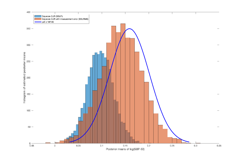
Figure 1: Posterior means of $\log$(SBP-50) for $\log$(weight) equation.

The results from the Bayesian estimation of SURME model (which accounts for the measurement error in the covariate SBP) is presented in the upper panel of Table 7. A quick glance shows that the results for the covariates measured without error are similar to those in Table 6, except for the intercept and the male indicator in the $\ln(weight)$ equation. The $\ln(height)$ coefficient in the $\ln(weight)$ equation is now slightly higher but its $95\%$ credible interval overlaps with that of the SUR model. Posterior estimates corresponding to transformed $SBP$ increase in both equations (from $0.097$ to $0.141$ in the $\ln(weight)$ equation and from $0.101$ to $0.152$ in the $HDL$ equation) leading to the following elasticities at the mean of the sample: $0.141$ and $0.115(=0.152/1.32)$, for weight and $HDL$, respectively. However, as the posterior standard errors become larger (from $0.027$ to $0.044$ in the $\ln(weight)$ equation and from $0.056$ to $0.092$ in the $HDL$ equation)—as in the Monte Carlo study—the $95\%$ HPDI of the posterior means of $\ln(SBP-50)$ overlap even if the distribution moves to the right when we go from SUR to SURME (see Figure 1). In particular, the $95\%$ HPDI of the posterior means of $\ln(SBP-50)$ are $\left[0.051;0.143\right]$ and $\left[0.009;0.194\right]$ in the $\ln(weight)$ and the $HDL$ equations, respectively, in the SUR model, and $\left[0.067;0.213\right]$ and $\left[0.005;0.304\right]$ in the $\ln(weight)$ and the $HDL$ equations in the SURME model. In the $HDL$ equation, the coefficient of SBP is positive but statistically equivalent to zero. Posterior estimate of measurement error variance is $0.029$, which leads to an estimated reliability ratio of about $59.78\%$ and a noise-to-true variance ratio of $67.27\%$. The posterior variances of the disturbances from $\ln(weight)$ and $HDL$ are close to those of SUR model and lead to an error correlation $\rho_{\varepsilon_{1}\varepsilon_{2}}=-0.25$. Inefficiency factors are close to 1 and Geweke’s CD confirms, for most parameters, that a sufficiently large number of draws has been taken.

The lower panel of Table 7 presents the results for the exposure equation from the Bayesian estimation of SURME model. In the first equation, only three variables have a positive effect on $\ln(SBP-50)$: $\ln(age)$, LDL20T and $\ln(height)$ (only at the $10\%$ probability level). In the second equation, four variables have a positive effect on $\ln(SBP-50)$: $\ln(age)$, LDL20T, male and smokers (the last two variables are different from zero only at the $10\%$ probability level).

We next estimate the SURME model using the MFVB approach, which takes $1565$ cycles to get the maximum of the evidence lower bound $l$. The results, presented in the upper panel of Table 8, shows that for the transformed SBP both the coefficient ($0.159$) and the probability interval ($\left[0.076;0.242\right]$) are similar to those obtained from the Bayesian estimation of SURME model. In the $HDL$ equation, the marginal effect at $0.186$ is higher compared to the Bayesian estimate, with a $95\%$ probability interval of $\left[0.03;0.34\right]$. Taking into account measurement errors using MFVB allows to get significantly larger and more accurate elasticities of weight ($0.159$) and $HDL$ ($0.1414=(0.186/1.32)$) for the transformed $SBP$ compared to the other method.

Posterior estimate of measurement error variance from the MFVB approach is $0.029$, which is similar to the Bayesian estimate, and leads to an estimated reliability ratio of about $60.2\%$ and to a noise-to-true variance ratio of $66.1\%$. The posterior variances of the disturbances from $\ln(weight)$ and $HDL$ are close to the Bayesian estimates and lead to the same correlation between the errors of the two equations $\rho_{\varepsilon_{1}\varepsilon_{2}}=-0.25$. The lower panel of Table 8 presents results for the exposure model estimated using with MFVB approximation method. In the first equation, four variables have a positive effect on $\ln(SBP-50)$: $\ln(age)$, smokers, $LDL20T$ and $\ln(height)$. Similarly, in the second equation four variables have a positive effect on $\ln(SBP-50)$: $\ln(age)$, $male$, $smokers$ and $LDL20T$. The exposure equation in the SURME model allows to define the implicit links between the true systolic blood pressure and the “risk factors” such as age, gender, smokers and “bad cholesterol” ($LDL20T$).

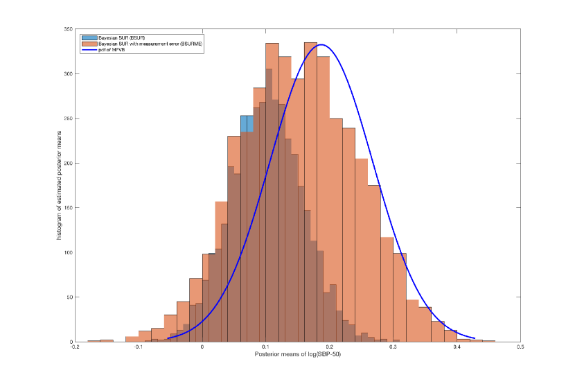
Figure 2: Posterior means of $\log$(SBP-50) for $\log$(HDL) equation.

Figure 1 gives the posterior densities of the parameter corresponding to $\ln(SBP-50)$ in the $\ln(weight)$ equation from the Bayesian estimation of SUR model, SURME model and the MFVB estimation of SURME model. We note a shift of the marginal effect of $\ln(SBP-50)$ on $\ln(weight)$ to the right of the distribution from a mode established around $0.097$ for SUR model to a mode of $0.141$ for SURME model but with a wider dispersion. The estimated probability density function (pdf) with MFVB is slightly to the right and centered around the mode ($0.159$) but with a surface under the curve globally equivalent to that of Bayesian estimation of SURME model. In Figure 2, we observe similar shifts in the posterior density of the parameter corresponding to $\ln(SBP-50)$ in the $HDL$ equation, when we move from SUR ($0.101$) to SURME ($0.152$) or to MFVB ($0.187$) estimation of SURME model.

We note that similar to the Monte Carlo study, the MFVB approach to estimating the SURME model improves the results compared to those from Gibbs sampling. The results actually lend credibility to the proposed MFVB algorithm since coefficient estimates for variables which do not have measurement error are almost unaltered. However, when measurement error in $SBP$ is ignored as in the SUR model, the posterior estimates are underestimated relative to the MFVB estimates. So, accounting for measurement error potentially corrects or reduces the bias in parameter estimates (see Carroll et al., 2006b).

6 Conclusion

The paper considers a SURME model (seemingly unrelated regression where some covariates have classical measurement error of the structural form) and introduces two novel estimation methods: a pure Bayesian algorithm based on MCMC and a second algorithm based on mean field variational Bayes approximation. The proposed algorithms use a prior distribution on measurement error variance to resolve identification issues in the model. In the MCMC estimation, Gibbs sampling is employed to sample the parameters from the conditional posterior distributions. While most of the conditional posterior densities have the standard form and are easily derived, the conditional posterior density for the true unobserved quantity associated with covariates having measurement error requires extensive attention to arrive at a manageable form. We also note that the proposed SURME model as explained is based on the structural form of measurement error, but the functional form of measurement error can be easily incorporated by introducing the distribution of the true unobserved quantity as a part of the subjective prior information. The expression for the joint and conditional posteriors will remain unchanged. However, estimating the SURME model using MCMC leads to high autocorrelation in the draws corresponding to the covariate measured with error. While this is easily dealt using thinning, the paper also proposes the MFVB approach as an alternative to get around the problem of high autocorrelation.

The proposed estimation algorithms are illustrated in multiple Monte Carlo simulation studies. While, the first set of 2 simulations (labeled Case I) investigate the effect on estimates by varying the variance of the true unobserved variable (for a fixed reliability ratio), the second set of 2 simulations examine the effect for a changing reliability ratio (for a fixed variance of the true unobserved variable). The results from all the simulations show that the Bayesian and MFVB estimation of SURME model reduce the biases to obtain satisfactory estimates as compared to estimates from SUR model. Moreover, the MFVB approach turns out as an excellent alternative to the MCMC and its poor mixing properties in the presence of latent variables. Besides, the MFVB approach has slightly better estimation accuracy and can be advantageous with large data sets.

The proposed models and techniques are also implemented in a health study where the two dependent variables, log of weight and high density lipoprotein (HDL), are regressed on a set of covariates measured without error and on systolic blood pressure (SBP) known to have measurement error. The model is estimated using the two algorithms and the results obtained reveal that the sign of the estimated coefficients are mostly consistent with what is typically found in the literature. Specifically, SBP has a positive effect on both $\ln(weight)$ and HDL, measurement error variance is small with an estimated reliability ratio of about $60\%$ and a noise-to-true variance ratio of $66\%$. To offer a baseline comparison, a SUR model that ignores measurement error in SBP is also estimated using Gibbs sampling. Comparing the results across models, we see that posterior estimates for covariates without measurement error are almost identical, but that of SBP is lower and hence underestimated both in the weight and the $HDL$ equations.

The combination of SUR and measurement error models is attractive and the proposed model can be generalized in several directions. One straightforward extension is the introduction of multiple covariates with measurement error in each SUR equation. However, the challenge here is to keep track of measurement errors arising from different covariates. The proposed SURME model can also be modified by introducing classical measurement error in the response variable or nonclassical measurement error models, where the errors may be correlated with the latent true values. Beyond the SUR models, these Bayesian approaches may be useful for measurement error in simultaneous equation models. We leave these possibilities for future research.

Table 1: Frequentist estimates of SUR Model. The table presents the true parameter values (true), regression coefficients (coef), relative error (re), standard error (se) and 95% confidence interval (inf, sup). $N=300$, $\sigma^{2}_{Z}=1$, $R_{Z}=0.8$, Replications=$100$.

	$\beta_{11}$	$\beta_{12}$	$\beta_{13}$	$\beta_{21}$	$\beta_{22}$	$\beta_{23}$	$\gamma_{1}$	$\gamma_{2}$	$\sigma_{11}$	$\sigma_{12}$	$\sigma_{22}$
true	3	5	4	4	3.8	3	4	4	1	0.5	1
coef	4.144	5.622	4.246	5.150	4.649	3.353	3.206	3.216	4.171	0.523	4.144
re	0.381	0.124	0.062	0.288	0.223	0.118	-0.198	-0.196	3.171	0.046	3.144
se	0.350	0.219	0.106	0.348	0.233	0.112	0.105	0.105
inf	3.458	5.192	4.038	4.467	4.192	3.134	3.000	3.010
sup	4.830	6.051	4.455	5.833	5.105	3.572	3.412	3.422

Table 2: Bayesian estimation of SURME model. The upper panel presents results for the main equations and the lower panel presents results for the exposure equations. mean is posterior mean, re is relative error, std is posterior standard deviation, if is inefficiency factor, and (inf-hpdi, sup-hpdi) represents 95% HPDI, and cd represents Geweke’s convergence diagnostics. $N=300$, $\sigma^{2}_{Z}=1$, $R_{Z}=0.8$, Draws=$51,000$, Burnin draws=$1,000$, thinning=$100$, Replications=$100$.

	$\beta_{11}$	$\beta_{12}$	$\beta_{13}$	$\beta_{21}$	$\beta_{22}$	$\beta_{23}$	$\gamma_{1}$	$\gamma_{2}$	$\sigma^{2}_{Z}$	$\sigma^{2}_{u}$	$\sigma_{11}$	$\sigma_{12}$	$\sigma_{22}$
true	3	5	4	4	3.8	3	4	4	1	0.25	1	0.5	1
mean	2.895	4.858	3.986	3.716	3.694	2.999	4.083	4.103	0.974	0.251	1.025	0.504	1.015
re	-0.035	-0.028	-0.004	-0.071	-0.028	-0.000	0.021	0.026	-0.026	0.005	0.025	0.008	0.015
std	0.369	0.243	0.119	0.376	0.261	0.125	0.131	0.130	0.071	0.020	0.187	0.135	0.184
if	1.029	1.028	1.023	1.055	1.066	1.050	1.117	1.232	1.032	1.011	1.011	1.004	1.013
inf-hpdi	2.280	4.450	3.786	3.086	3.257	2.790	3.870	3.893	0.862	0.220	0.752	0.297	0.746
sup-hpdi	3.494	5.251	4.180	4.320	4.114	3.202	4.301	4.320	1.093	0.284	1.359	0.738	1.347
cd	0.990	0.980	1.000	0.970	0.950	0.980	0.990	0.950	0.960	0.990	0.990	0.960	0.970

	$\omega_{11}$	$\omega_{12}$	$\omega_{13}$	$\omega_{21}$	$\omega_{22}$	$\omega_{23}$
true	1.5	0.75	0.3	1.5	1.05	0.45
mean	1.466	0.773	0.307	1.489	1.068	0.443
re	-0.023	0.031	0.022	-0.007	0.017	-0.016
std	0.165	0.109	0.055	0.166	0.109	0.055
if	1.000	1.001	1.001	1.001	1.004	1.000
inf-hpdi	1.194	0.593	0.216	1.214	0.888	0.353
sup-hpdi	1.735	0.952	0.396	1.758	1.246	0.533
cd	0.990	0.990	0.990	0.970	0.980	0.980

Table 3: MFVB estimation of SURME model. The upper panel presents results for the main equations and the lower panel presents results for the exposure equations. mean is posterior mean, re is relative error, std is posterior standard deviation, and (inf-cri, sup-cri) represents 95% credible interval. $N=300$, $\sigma^{2}_{Z}=1$, $R_{Z}=0.8$, Replications=$100$, Cycles = $145.49$, Maximum Elbo = $-3517.205$.

	$\beta_{11}$	$\beta_{12}$	$\beta_{13}$	$\beta_{21}$	$\beta_{22}$	$\beta_{23}$	$\gamma_{1}$	$\gamma_{2}$	$\sigma^{2}_{Z}$	$\sigma^{2}_{u}$	$\sigma_{11}$	$\sigma_{12}$	$\sigma_{22}$
true	3	5	4	4	3.8	3	4	4	1	0.25	1	0.5	1
mean	2.968	4.908	4.006	3.889	3.823	3.054	4.027	3.990	1.004	0.241	1.089	0.534	1.098
re	-0.011	-0.018	0.002	-0.028	0.006	0.018	0.007	-0.003	0.004	-0.035	0.089	0.067	0.098
std	0.149	0.103	0.045	0.149	0.103	0.045	0.065	0.055	0.058	0.014	0.083	0.065	0.084
inf-cri	2.677	4.707	3.918	3.596	3.621	2.965	3.898	3.882	0.890	0.214	0.926	0.405	0.934
sup-cri	3.259	5.110	4.095	4.181	4.026	3.143	4.155	4.097	1.118	0.269	1.251	0.662	1.262

	$\omega_{11}$	$\omega_{12}$	$\omega_{13}$	$\omega_{21}$	$\omega_{22}$	$\omega_{23}$
true	1.5	0.75	0.3	1.5	1.05	0.45
mean	1.468	0.771	0.306	1.487	1.066	0.442
re	-0.021	0.029	0.019	-0.009	0.015	-0.017
std	0.151	0.099	0.050	0.151	0.099	0.050
inf-cri	1.172	0.577	0.208	1.191	0.871	0.344
sup-cri	1.765	0.966	0.403	1.784	1.261	0.540

Table 4: Summary table showing relative errors of the parameters for all simulations from the frequentist estimation of SUR model, Bayesian estimation of SURME model, and MFVB estimation of SURME model.

			$\beta_{11}$	$\beta_{12}$	$\beta_{13}$	$\beta_{21}$	$\beta_{22}$	$\beta_{23}$	$\gamma_{1}$	$\gamma_{2}$	$\sigma^{2}_{Z}$	$\sigma^{2}_{u}$	$\sigma_{11}$	$\sigma_{12}$	$\sigma_{22}$
	sur		0.381	0.124	0.062	0.288	0.223	0.118	-0.198	-0.196			3.171	0.046	3.144
$(\sigma_{Z}^{2}=1,R_{Z}=0.8)$	surme		-0.035	-0.028	-0.004	-0.071	-0.028	0.000	0.021	0.026	-0.026	0.005	0.025	0.008	0.015
	mfvb		-0.011	-0.018	0.002	-0.028	0.006	0.018	0.007	-0.003	0.004	-0.035	0.089	0.067	0.098
	sur		0.386	0.118	0.059	0.282	0.213	0.113	-0.195	-0.190			0.195	0.002	0.187
$(\sigma_{Z}^{2}=0.0625,R_{Z}=0.8)$	surme		-0.294	-0.096	-0.045	-0.256	-0.186	-0.099	0.150	0.168	-0.123	0.433	-0.079	-0.008	-0.090
	mfvb		-0.170	-0.056	-0.025	-0.111	-0.077	-0.039	0.086	0.070	-0.049	0.174	-0.026	0.011	-0.027
	sur		0.834	0.263	0.130	0.627	0.481	0.255	-0.427	-0.426			6.796	0.088	6.793
$(\sigma_{Z}^{2}=1,R_{Z}=0.5714)$	surme		-0.065	-0.078	-0.013	-0.151	-0.070	-0.003	0.053	0.058	-0.081	0.010	0.023	0.005	0.020
	mfvb		-0.001	-0.046	0.004	-0.064	0.004	0.039	0.012	-0.002	0.000	-0.016	0.081	0.069	0.097
	sur		0.844	0.256	0.128	0.625	0.468	0.251	-0.425	-0.419			0.424	0.000	0.413
$(\sigma_{Z}^{2}=0.0625,R_{Z}=0.5714)$	surme		-0.317	-0.107	-0.050	-0.283	-0.205	-0.107	0.164	0.184	-0.154	0.154	-0.070	-0.023	-0.087
	mfvb		-0.166	-0.057	-0.025	-0.109	-0.072	-0.035	0.085	0.066	-0.055	0.042	-0.019	0.003	-0.016

Table 5: Health application - variable definitions and data summary.

variable		description	mean	std
$\ln$(weight)		Logarithm of weight (in kilograms).	$4.40$	$0.24$
HDL		High density lipoprotein (mmol/l, millimoles per litre).	$1.32$	$0.45$
$\ln$(age)		Logarithm of age (in years).	$4.00$	$0.15$
Male		Indicator variable for male.	$0.57$	$0.49$
Smokers		Indicator variable for individuals who smoke daily or some days.	$0.46$	$0.50$
Sedentary		Number of hours of sedentary activities.	$5.28$	$3.37$
Sleep disorder		Indicator variable for sleep disorder problem.	$0.11$	$0.32$
LDL20T		Low density lipoprotein plus 20 percent of Triglyceride (mmol/l, millimoles per litre).	$3.94$	$1.09$
$\ln$(SBP-50)		Transformation on systolic blood pressure.	$4.28$	$0.24$

Table 6: Health application - Bayesian estimation of SUR model. The table presents the posterior mean (mean), standard deviation (std), inefficiency factor (if), and Geweke’s convergence diagnostics (cd) of the parameters. Draws=$450,000$, Burnin draws=$50,000$, thinning=$100$.

	$\ln(weight)$					$HDL$
	mean	std	if	cd		mean	std	if	cd
Intercept	-3.4956	0.5894	0.9850	0.5770		1.1074	0.3665	0.9995	0.1262
$\ln(age)$	-0.0497	0.0443	1.0089	-0.3950		0.1035	0.0880	0.9869	0.4550
Male	0.0406	0.0154	0.9914	-0.8753		-0.2794	0.0264	0.9930	-1.0020
Smokers	-0.1008	0.0132	0.9908	0.5216		0.0424	0.0275	0.9870	1.0594
Sedentary	0.0085	0.0019	0.9821	-0.2897		-0.0076	0.0039	1.0069	-0.4709
Sleep disorder	0.1061	0.0202	1.0197	-0.1130		-0.0272	0.0412	0.9903	0.2408
LDL20T	0.0223	0.0058	1.0098	-0.4155		-0.1137	0.0119	1.0024	-0.1327
$\ln(height)$	1.4731	0.1134	0.9949	-0.6200
$\ln(SBP-50)$	0.0967	0.0277	0.9963	0.8784		0.1012	0.0560	0.9873	-0.7712
$\sigma_{11}$	0.0399	0.0018	0.9900	-1.0924
$\sigma_{12}$	-0.0250	0.0027	1.0219	0.4914
$\sigma_{22}$	0.1693	0.0075	1	-0.5193

Table 7: Health application - Bayesian estimation of SURME model. The upper panel presents results for the main equations and the lower panel presents results for the exposure equations. mean is posterior mean, std is posterior standard deviation, if is inefficiency factor, and cd is Geweke’s convergence diagnostics. Draws=$450,000$, Burnin draws=$50,000$, thinning=$100$.

	$log(weight)$					$HDL$
	mean	std	if	cd		mean	std	if	cd
Intercept	-5.2859	0.8284	1.0132	0.6022		1.1825	0.4332	1.7579	0.7772
$\ln(age)$	-0.0383	0.0521	1.1769	0.7601		0.0329	0.0997	1.4330	1.7639
Male	0.0156	0.0187	1.0181	-0.0596		-0.2807	0.0276	1.0156	0.7971
Smokers	-0.1009	0.0146	0.9998	0.8830		0.0375	0.0280	1.0110	1.7027
Sedentary	0.0080	0.0021	1.0279	0.8739		-0.0075	0.0040	1.0071	-0.1389
Sleep disorder	0.1066	0.0222	0.9863	0.8386		-0.0294	0.0425	0.9941	-0.0086
LDL20T	0.0224	0.0066	1.0159	1.4224		-0.1155	0.0126	1.0008	-0.1091
$\ln(height)$	1.7790	0.1561	1.0112	-0.4465
$\ln(SBP-50)$	0.1416	0.0443	3.3261	-0.6761		0.1520	0.0921	3.8691	-1.1416
$\sigma_{11}$	0.0485	0.0022	0.9933	0.1713
$\sigma_{12}$	-0.0252	0.0030	0.9829	-0.7013
$\sigma_{22}$	0.1778	0.0080	1.0163	-0.3718
$\sigma^{2}_{Z}$	0.0440	0.0019	1.0025	0.9275
$\sigma^{2}_{u}$	0.0296	0.0016	1.0275	-1.4186
	$\ln(SBP-50)$					$\ln(SBP-50)$
	mean	std	if	cd		mean	std	if	cd
Intercept	1.1847	0.7160	1.0137	-0.0465		2.4526	0.2377	1.0053	0.8891
$\ln(age)$	0.4156	0.0577	1.0250	0.8542		0.4302	0.0580	1.0051	-0.8192
Male	0.0118	0.0201	0.9935	-0.0731		0.0318	0.0172	1.0165	-0.4137
Smokers	0.0341	0.0180	1.0020	0.6742		0.0363	0.0179	1.0280	-1.3321
Sedentary	-0.0018	0.0026	0.9709	0.1812		-0.0013	0.0025	0.9886	1.3253
Sleep disorder	0.0087	0.0277	0.9841	-0.2518		0.0094	0.0274	1.0220	0.8595
LDL20T	0.0185	0.0079	1.0111	-0.1604		0.0190	0.0080	1.0092	-0.8225
$\ln(height)$	0.2620	0.1405	1.0129	-0.2297

Table 8: Health application - MFVB estimation of SURME model. Cycles=$1565$, Maximum Elbo =$-9076.16$. The upper panel presents results for the main equations and the lower panel presents results for the exposure equations. mean is posterior mean and std is posterior standard deviation of the parameters.

	$\ln(weight)$			$HDL$
	mean	std		mean	std
Intercept	-5.3245	0.8069		1.0892	0.3726
$\ln(age)$	-0.0461	0.0477		0.0199	0.0908
Male	0.0148	0.0185		-0.2816	0.0272
Smokers	-0.1018	0.0144		0.0364	0.0276
Sedentary	0.0080	0.0021		-0.0075	0.0040
Sleep disorder	0.1066	0.0222		-0.0293	0.0425
LDL20T	0.0222	0.0064		-0.1160	0.0123
$\ln(height)$	1.7781	0.1537
$\ln(SBP-50)$	0.1594	0.0422		0.1867	0.0808
$\sigma_{11}$	0.0484	0.0022
$\sigma_{12}$	-0.0252	0.0030
$\sigma_{22}$	0.1778	0.0079
$\sigma^{2}_{Z}$	0.0443	0.0014
$\sigma^{2}_{u}$	0.0293	0.0009
	$\ln(SBP-50)$			$\ln(SBP-50)$
	mean	std		mean	std
Intercept	1.1679	0.6340		2.4525	0.1843
$\ln(age)$	0.4153	0.0451		0.4305	0.0449
Male	0.0118	0.0165		0.0318	0.0136
Smokers	0.0340	0.0138		0.0362	0.0138
Sedentary	-0.0018	0.0020		-0.0012	0.0020
Sleep disorder	0.0090	0.0213		0.0095	0.0213
LDL20T	0.0186	0.0061		0.0187	0.0061
$\ln(height)$	0.2655	0.1228

References

- Ando and Zellner (2010) Ando, T. and Zellner, A. (2010), “Hierarchical Bayesian Analysis of the Seemingly Unrelated Regression and Simultaneous Equation Models using a Combination of Direct Monte Carlo and Importance Sampling Techniques,” Bayesian Analysis, 5, 65–95.
- Bishop (2006) Bishop, C. M. (2006), Pattern Recognition and Machine Learning, Springer, New York.
- Blei et al. (2017) Blei, D. M., Kuckelbir, A., and McAuliffe, J. D. (2017), “Variational Inference: A Review for Statisticians,” Journal of the American Statistical Association, 112, 859–877.
- Carroll et al. (2006a) Carroll, R. J., Ruppert, D., Stefanski, L. A., and Crainiceanu, C. M. (2006a), Measurement Error in Nonlinear Models: A Modern Perspective, Chapman & Hall, Boca Raton.
- Carroll et al. (2006b) Carroll, R. J., Midthune, D., Freedman, L. S., and Kipnis, V. (2006b), “Seemingly Unrelated Measurement Error Models with Application to Nutritional Epidemiology,” Biometrics, 62, 75–84.
- Casella and George (1992) Casella, G. and George, E. I. (1992), “Explaining the Gibbs Sampler,” The American Statistician, 46, 167–174.
- Celeux et al. (2006) Celeux, G., Forbes, F., Robert, C. P., and Titterington, D. M. (2006), “Deviance Information Criteria for Missing Data Models,” Bayesian Analysis, 1, 651–674.
- Chan and Grant (2016) Chan, J. and Grant, A. D. (2016), “Fast Computation of the Deviance Information Criterion for Latent Variable Models,” Computational Statistics and Data Analysis, 100, 847–859.
- Cheng and Van Ness (1999) Cheng, C.-L. and Van Ness, J. W. (1999), Statistical Regression with Measurement Error, Arnold Publishers, London.
- Cheng et al. (2014) Cheng, C.-L., Shalabh, and Garg, G. (2014), “Coefficient of Determination for Multiple Measurement Error Models,” Journal of Multivariate Analysis, 126, 137–152.
- Chib and Greenberg (1995) Chib, S. and Greenberg, E. (1995), “Hierarchical Analysis of SUR Models with Extension to Correlated Serial Errors and Time-Varying Parameter Models,” Journal of Econometrics, 68, 339–360.
- Faes et al. (2011) Faes, C., Ormerod, J. T., and Wand, M. P. (2011), “Variational Bayesian Inference for Parametric and Nonparametric Regression With Missing Data,” Journal of the American Statistical Association, 106, 959–971.
- Fiebig (2001) Fiebig, D. G. (2001), “Seemingly Unrelated Regression,” in A Companion to Theoretical Econometrics, ed. B. H. Baltagi, pp. 101–121, Blackwell Publishing, Massachusett.
- Fuller (1987) Fuller, W. A. (1987), Measurement Error Models, John Wiley & Sons, New York.
- Geman and Geman (1984) Geman, S. and Geman, D. (1984), “Stochastic Relaxation, Gibbs Distributions, and the Bayesian Restoration of Images,” IEEE Transactions on Pattern Analysis and Machine Intelligence, 6, 721–741.
- Geyer (1991) Geyer, C. J. (1991), “Markov chain Monte Carlo Maximum Likelihood,” in Computing Science and Statistics: Proceedings of the 23rd Symposium on the Interface, ed. E. M. Kemramides, pp. 156–163, Interface Foundation of North America, Fairfax Station, VA, USA.
- Giordano et al. (2018) Giordano, R., Broderick, T., and Jordan, M. I. (2018), “Covariances, Robustness and Variational Bayes,” Journal of Machine Learning Research, 19, 1–49.
- Griffiths and Chotikapanich (1997) Griffiths, W. E. and Chotikapanich, D. (1997), “Bayesian Methodology for Imposing Inequality Constraints on a Linear Expenditure System with Demographic Factors,” Australian Economic Papers, 36, 321–341.
- Griffiths and Valenzuela (2006) Griffiths, W. E. and Valenzuela, M. R. (2006), “Gibbs Samplers for a set of Seemingly Unrelated Regressions,” Australian & New Zealand Journal of Statistics, 48, 335–351.
- Hu and Wansbeek (2017) Hu, Y. and Wansbeek, T. (2017), “Measurement Error Models: Editor’s Introduction,” Journal of Econometrics, 200, 151–153.
- Jeliazkov (2013) Jeliazkov, I. (2013), “Nonparametric Vector Autoregressions: Specification, Estimation and Inference,” Advances in Econometrics, 32, 327–359.
- Kannel et al. (1986) Kannel, W. B., Neaton, J. D., Wentworth, D., Thomas, H. E., Stamler, J., Hulley, S. B., and Kjelsberg, M. O. (1986), “Overall and Coronary Heart Disease Mortality Rates in Relation to Major Risk Factors in 325,348 men Screened for the MRFIT,” American Heart Journal, 112, 825–836.
- Koop et al. (2005) Koop, G., Poirier, D. J., and Tobias, J. (2005), “Semiparametric Bayesian Inference in Multiple Equation Models,” Journal of Applied Econometrics, 20, 723–747.
- Lee and Wand (2016) Lee, C. Y. Y. and Wand, M. P. (2016), “Streamlined Mean Field Variational Bayesian Inference in Multiple Equation Models,” Biometrical Journal, 58, 868–895.
- Link and Eaton (2012) Link, W. A. and Eaton, M. J. (2012), “On Thinning of Chains in MCMC,” Methods in Ecology and Evolution, 3, 112–115.
- Liu (1994) Liu, J. S. (1994), “The Collapsed Gibbs Sampler in Bayesian Computations with Applications to a Gene Regulation Problem,” Journal of the American Statistical Association, 89, 958–966.
- Liu and Liang (1992) Liu, X. and Liang, K.-Y. (1992), “Efficacy of Repeated Measures in Regression Models with Meausrement Error,” Biometrics, 48, 645–654.
- MacEachern and Berliner (1994) MacEachern, S. N. and Berliner, L. M. (1994), “Subsampling the Gibbs Sampler,” The American Statistician, 48, 188–190.
- Ormerod and Wand (2010) Ormerod, J. T. and Wand, M. P. (2010), “Explaining Variational Approximations,” The American Statistician, 64, 140–153.
- Owen (2017) Owen, A. B. (2017), “Statistically Efficient Thinning of a Markov Chain Sampler,” Journal of Computational and Graphical Statistics, 26, 738–744.
- Percy (1992) Percy, D. F. (1992), “Prediction for Seemingly Unrelated Regressions,” Journal of the Royal Statistical Society – Series B, 54, 243–252.
- Pham et al. (2013) Pham, T. H., Ormerod, J. T., and Wand, M. P. (2013), “Mean Field Variational Bayesian Inference for Nonparametric Regression with Measurement Error,” Computational Statistics and Data Analysis, 68, 375–387.
- Rao et al. (2008) Rao, C. R., Toutenburg, H., Shalabh, and Heumann, C. (2008), Linear Models and Generalizations: Least Squares and Alternatives, Springer, Berlin.
- Shalabh (2003) Shalabh (2003), “Consistent Estimation of Coefficients in Measurement Error Models with Replicated Observations,” Journal of Multivariate Analysis, 86, 227–241.
- Spiegelhalter et al. (2002) Spiegelhalter, D. J., Best, N. G., Carlin, B. P., and van der Linde, A. (2002), “Bayesian Measures of Model Complexity and Fit,” Journal of the Royal Statistical Society – Series B, 64, 583–639.
- Spiegelhalter et al. (2014) Spiegelhalter, D. J., Best, N. G., Carlin, B. P., and van der Linde, A. (2014), “The Deviance Information Criterion: 12 years on,” Journal of the Royal Statistical Society – Series B, 76, 485–493.
- Srivastava and Dwivedi (1979) Srivastava, V. K. and Dwivedi, T. D. (1979), “Estimation of Seemingly Unrelated Regression Equations,” Journal of Econometrics, 10, 15–32.
- Srivastava and Giles (1987) Srivastava, V. K. and Giles, D. E. A. (1987), Seemingly Unrelated Regression Equations Models: Estimation and Inference, Marcel Dekker, New York.
- Steel (1992) Steel, M. F. J. (1992), “Posterior Analysis of Restricted Seemingly Unrelated Regression Equation Models: A Recursive Analytical Approach,” Econometric Reviews, 11, 129–142.
- Tao et al. (2011) Tao, G., Chen, Y., Wen, C., and Bi, M. (2011), “Statistical Analysis of Blood Pressure Measurement Errors by Oscillometry during Surgical Operations,” Blood Pressure Monitoring, 16, 285–290.
- van Dyk and Park (2008) van Dyk, D. A. and Park, T. (2008), “Partially Collapsed Gibbs Samplers: Theory and Methods,” Journal of the American Statistical Association, 103, 790–796.
- Wansbeek and Meijer (2000) Wansbeek, T. and Meijer, E. (2000), Meausrement Error and Latent Variables in Econometrics, Noth Holland, Amsterdam.
- Yang et al. (2018) Yang, Y., Pati, D., and Bhattacharya, A. (2018), “ Variational Inference with Statistical Guarantees,” https://arxiv.org/abs/1710.03266.
- Zellner (1962) Zellner, A. (1962), “An Efficient Method of Estimating Seemingly Unrelated Regression and Tests for Aggregation Bias,” Journal of the American Statistical Association, 57, 348–368.
- Zellner (1971) Zellner, A. (1971), An Introduction to Bayesian Inference in Econometrics, John Wiley & Sons, New York.
- Zellner and Ando (2010) Zellner, A. and Ando, T. (2010), “A Direct Monte Carlo Approach for Bayesian Analysis of the Seemingly Unrelated Regression Model,” Journal of Econometrics, 159, 33–45.