Structural Patterns and Generative Models of Real-world Hypergraphs

Abstract.

Graphs have been utilized as a powerful tool to model pairwise relationships between people or objects. Such structure is a special type of a broader concept referred to as hypergraph, in which each hyperedge may consist of an arbitrary number of nodes, rather than just two. A large number of real-world datasets are of this form – for example, lists of recipients of emails sent from an organization, users participating in a discussion thread or subject labels tagged in an online question. However, due to complex representations and lack of adequate tools, little attention has been paid to exploring the underlying patterns in these interactions.

In this work, we empirically study a number of real-world hypergraph datasets across various domains. In order to enable thorough investigations, we introduce the multi-level decomposition method, which represents each hypergraph by a set of pairwise graphs. Each pairwise graph, which we refer to as a $k$-level decomposed graph, captures the interactions between pairs of subsets of $k$ nodes. We empirically find that at each decomposition level, the investigated hypergraphs obey five structural properties. These properties serve as criteria for evaluating how realistic a hypergraph is, and establish a foundation for the hypergraph generation problem. We also propose a hypergraph generator that is remarkably simple but capable of fulfilling these evaluation metrics, which are hardly achieved by other baseline generator models.

1. Introduction

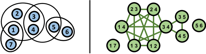
Figure 1. A hypergraph and its $2$-level decomposed graph.

Edge Level		Triangle Level		4clique Level
Real Data	HyperPA (Proposed)	Real Data	HyperPA (Proposed)	Real Data	HyperPA (Proposed)
NaivePA	SubsetSamplling	NaivePA	SubsetSampling	NaivePA	SubsetSampling

Figure 2. Comparison of hypergraph generators with respect to degree distributions of decomposed graphs at different decomposition levels. The hypergraph generated by HyperPA resembles the real data most. See Sect. 5.4 for numerical analysis.

In our digital age, interactions that involve a group of people or objects are ubiquitous (Benson et al., 2018a; Benson et al., 2018b, 2016). These associations arise from various domains, ranging from academic communities, online social networks to pharmaceutical practice. In particular, research papers are often published by the collaborations of several coauthors, social networks involve group communications, and several related medications may be applied as a treatment rather than just two.

Such structures can be represented as hypergraphs (C, 2013; Bonacich et al., 2004), which is a generalization of the usual notion of graphs. In hypergraphs, each node can be a person or an object. However, each hyperedge acts as an interaction of an arbitrary number of nodes. For example, if each node represents an author, a hyperedge can be treated as a research paper which was published by a group of authors. A hyperedge also reveals the subset interactions among the elements of each subset, which this work pays special attention to. A subset interaction among nodes (e.g., $\{a,b\}$) is defined as their co-appearance as a subset of a hyperedge (e.g., $\{a,b,c,d\}$). The freedom of number of nodes involved in each hyperedge and subset interactions naturally contribute to the complexity of hypergraphs.

While pairwise graphs have been extensively studied in terms of mining structures (Milo et al., 2002; Broder et al., 2000; Girvan and Newman, 2002), discovering hidden characteristics (Faloutsos et al., 1999; Bollobás and Riordan, 2004; Eikmeier and Gleich, 2017; Kleinberg et al., 1999) as well as evolutionary patterns (Paranjape et al., 2017; Leskovec et al., 2008; Leskovec et al., 2005), little attention has been paid to defining and addressing analogous problems in hypergraphs. Due to the complexity of subset interactions, any single representation of hypergraphs relying on pairwise links would suffer from information loss. Given that most existing graph data structures only capture relationships between pairs of nodes, and more importantly, most patterns discovered are based on pairwise links-based measurements, directly applying the existing results in pairwise graphs to hypergraphs constitutes a challenge.

Here we investigate several hypergraph datasets among various domains (Benson et al., 2018a; Sinha et al., 2015; Yin et al., 2017). We introduce the multi-level decomposition of hypergraphs, which captures relationships between subsets of nodes. This offers a set of pairwise link representations convenient for analysis while guaranteeing to recover the original hypergraphs. In the most elementary type of decomposition, referred to as “node-level decomposed graph” in this paper, two nodes are linked if they appear in at least one hyperedge together. This is the decomposition for $k=1$. In the $k$-level decomposed graph, a node is defined as a set of $k$ nodes in the original hypergraph, and two nodes are connected if their union appears in a hyperedge (see Fig. 1).

Using the multi-level decomposition, we find that the decomposed graphs of thirteen real-world hypergraphs generally obey the following well-known properties of real-world graphs, across different levels: (1) giant connected components, (2) heavy-tailed degree distributions, (3) small effective diameters, (4) high clustering coefficients, and (5) skewed singular-value distributions. This decomposition also reveals how well such subset interactions are connected, and this connectivity varies across different domains.

What could be the possible underlying principles for such patterns? Driven by this question, we propose a simple hypergraph generator model called HyperPA. By some proper modifications of preferential attachment (Barabási and Albert, 1999; Albert et al., 2002; Kleinberg et al., 1999), which account for degree as a group, nodes can “get rich” together while maintaining subset interactions. Compared to two other baseline models, HyperPA shows more realistic results in reproducing the patterns discovered in real-world hypergraphs and resembling the connectivity of such subset interactions (see Fig. 2).

Findings in common properties of real-world hypergraphs and their underlying explanations can be significant for several reasons: (1) anomaly detection: if some data significantly deviates from the set of common patterns, it is reasonable to raise an alarm for anomalies, (2) anonymization: by fully reproducing these patterns, organizations may synthesize datasets to avoid disclosing important internal information. (3) simulation: generated hypergraphs can be utilized for “what-if” simulation scenarios when collecting large-size hypergraph datasets is costly and difficult.

In short, the main contributions of our paper are three-fold.

• Multi-level decomposition: a tool that facilitates easy and comprehensive analysis of subset interactions in hypergraphs.

• Patterns: five structural properties that are commonly held in thirteen real-world hypergraphs from diverse domains.

• Hypergraph generator (HyperPA): a simple but powerful model that produces hypergraphs satisfying the above properties.

Reproducibility: We made the datasets, the code, and the full experimental results available at https://github.com/manhtuando97/KDD-20-Hypergraph.

The remaining sections of this paper are outlined as follow: Sect. 2 provides a brief survey of related work. In Sect. 3, we introduce our decomposition tool which facilitates our understanding of structural properties of hypergraphs. Our empirical findings on real-world hypergraph datasets are presented in Sect. 4. Sect. 5 introduces hypergraph generators and demonstrates how these models perform in terms of reproducing the real-world patterns. We discuss and conclude our work in Sect. 6.

2. Background and Related Work

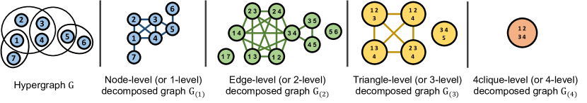
Figure 3. Pictorial description of multi-level decomposition of a hypergraph $G$. Each $k$-level decomposed graph reveals interactions between subsets of $k$ nodes.

Graph properties: Many empirical studies have been conducted to explore common properties of real-world pair-wise graphs based on predefined measurements (Easley et al., 2010). There are two main types of these properties: static and dynamic. Static properties are revealed from a snapshot of the graphs at a particular time, and they include degree distribution (Abello et al., 1998; Faloutsos et al., 1999), diameter (Bollobás and Riordan, 2004; Abello et al., 2013), distribution of eigenvalues (Eikmeier and Gleich, 2017), and more (Yin et al., 2017; Shin et al., 2018; Kleinberg et al., 1999; Milgram, 1967; Chung and Lu, 2002; Broder et al., 2000; Bollobás and Riordan, 2004; Albert et al., 1999; Kleinberg, 2002; Akoglu et al., 2010). Dynamic properties examine the evolution of a graph over a period of time. Real-world graphs are found to possess an increasing average degree and a shrinking diameter (Leskovec et al., 2005). Other dynamic properties include short distances of spanning new edges (Leskovec et al., 2008), temporal locality in triangle formation (Shin, 2017), and temporal network motifs (Paranjape et al., 2017; Liu et al., 2019).

Graph generative models: In conjunction, numerous graph generator models have been developed to produce synthetic graphs satisfying these commonly held patterns. Some of them focus on reproducing realistic degree distributions (Cooper and Frieze, 2003; Barabási and Albert, 1999; Mitzenmacher, 2004; Mahadevan et al., 2006). Others exploit locality to generate communities within the graph (Kumar et al., 2000; Kleinberg et al., 1999; Kolda et al., 2014; Vázquez, 2003; Watts and Strogatz, 1998; Newman, 2001). In (Leskovec et al., 2005; Akoglu et al., 2008), dynamic patterns of graph evolution are recaptured. While most of these stochastic generator models rely on empirical results to demonstrate their abilities to repeat realistic behavior, (Leskovec et al., 2010; Akoglu et al., 2008) provide theoretical guarantees. Although most of the aforementioned graph generators are self-contained stochastic models, several models require some explicit fitting to real data in order to exactly reproduce the patterns (Sala et al., 2010; Edunov et al., 2016; Leskovec et al., 2010).

Hypergraphs: Hypergraphs are used for representing various entities in diverse fields, including biology, medicine, social networks, and web (Benson et al., 2018a; Benson et al., 2016; Akoglu et al., 2008). To better analyze and process hypergraphs, there has been an increasing interest in extending studies on graphs to hypergraphs, including spectral theory (Zhou et al., 2006; Kleinberg et al., 1999) and triadic closure theory (Benson et al., 2018a). Studies have also proposed models of the generation and evolution of hyperedges (Benson et al., 2018b; Benson et al., 2018a; Stasi et al., 2014; Chodrow, 2019). However, (Benson et al., 2018b) focuses on repeat patterns of hyperedges, particularly on the recency bias and intensity of repeats, and generates only the next hyperedge, given all previous hyperedges. (Benson et al., 2018a) focuses on a particular type of hypergraph dynamics, namely simplicial closure. On the other hand, (Stasi et al., 2014) and (Chodrow, 2019) try to configure the generated hypergraphs to satisfy a given degree distribution without explicitly accounting for subset interactions in exploring the patterns.

In our work, we study the general patterns of real-world hypergraphs, encompassing the wide range of extensions studied in graphs with a strong emphasis on ‘subset interactions’. On such basis, we propose and evaluate generative models for hypergraphs.

3. Multi-level Decomposition

In this section, we introduce the multi-level decomposition, which is our method for analyzing hypergraphs. Our motivation for the multi-level decomposition is that it is not straightforward to investigate the properties of hypergraphs in their raw form. We instead seek a way to analyze hypergraphs through the lens of ordinary graphs. By transforming hypergraphs into graphs, we can adopt the various properties studied in graphs for hypergraphs.

Hypergraphs and subset interactions: A hypergraph is defined as $G=(V,E)$, where $V$ is a set of nodes and $E\subset 2^{V}$ is a set of hyperedges. Each hyperedge $e\subseteq V$ is a set of $|e|$ nodes that have appeared as a group. Distinguished from hyperedges, a subset interaction among two or more nodes indicates their co-appearance as a subset of a hyperedge. For example, a hyperedge $\{a,b,c,d\}$ leads to the following subset interactions: $\{a,b,c,d\}$, $\{a,b,c\}$, $\{b,c,d\}$, $\{c,d,a\}$, $\{d,a,b\}$, $\{a,b\}$, $\{a,c\}$, $\{a,d\}$, $\{b,c\}$, $\{b,d\}$, and $\{c,d\}$.

Multi-level decomposition: Given a hypergraph $G=(V,E)$, the multi-level decomposition of $G$ is defined as a set of $k$-level decomposed graphs for every $k\in\{1,...,\max_{e\in E}(|e|)\}$, where $\max_{e\in E}(|e|)\}$ is the maximum size of a hyperedge in $E$. The $k$-level decomposed graph, which is illustrated in Fig. 3, is defined below.

Definition 1 ($k$-level decomposed graph). The $\mathit{k}$-level decomposed graph of a hypergraph $G=(V,E)$ is $G_{(k)}=(V_{(k)},E_{(k)})$ where

$$V_{(k)}:=\{v_{(k)}\in 2^{V}:|v_{(k)}|=k\text{ and }\exists e\in E\text{ s.t. }v_{(k)}\subseteq e\},$$

$${E_{(k)}:=\{\{u_{(k)},v_{(k)}\}\in\binom{V_{(k)}}{2}:\exists e\in E\text{ s.t. }u_{(k)}\cup v_{(k)}\subseteq e\}.}$$

The nodes in the $k$-level decomposed graph $G_{(k)}$ of a hypergraph $G$ are the sets of $k$ nodes in $G$ that appear together in at least one hyperedge in $G$. In $G_{(k)}$, two sets of $k$ nodes are connected by an edge if and only if there exists a hyperedge in $G$ that contains both. That is, the $k$-level decomposed graph naturally represents how each set of $k$ nodes interacts, as a group, with other sets of $k$ nodes. Utilizing decomposed graphs constitutes several advantages:

• Subset interaction: decomposed graphs reveal subset interactions between subsets of nodes.

• Pairwise graph representation: decomposed graphs can be easily analyzed with existing measurements for pairwise graphs.

• No information loss: the original hypergraph can be recovered from the decomposed graphs (see Appendix C.1).

Notice that the notion of $k$-level decomposition is a generalization of an existing concept: when $k=1$, the decomposed graph corresponds to the widely-used pairwise projected graph.

In our study, we focus on $k$-level decomposed graphs with $k\in\{1,2,3,4\}$, as most hyperedges in real-world hypergraphs are of sizes only up to $4$. For simplicity, we call them node-level, edge-level, triangle-level, and 4clique-level decomposed graphs, respectively.

4. Observations

In this section, we demonstrate that the following structural patterns hold in each level of decomposed graphs of real hypergraphs^,:

• P1. Giant connected component

• P2. Heavy-tailed degree distribution

• P3. Small effective diameter

• P4. High clustering coefficient

• P5. Skewed singular values

These patterns, which are described in detail in the following subsections, are supported by our observations in thirteen real hypergraph datasets of medium to large sizes. Details on the datasets can be found in Appendix A, and the complete set of observations is available in (app, 2020). Below, we provide the intuition behind them and present a random hypergraph model that we use as the null model.

Intuition behind the patterns. Consider the coauthorship data as an example: in our node-level decomposed graph, each node represents an author, and two nodes are connected if and only if these two authors have coauthored at least one paper before. Therefore, this node-level decomposition can be interpreted as an author network. Such node-level decomposed graphs are not “real” graphs since they are obtained by decomposing the original hypergraphs. However, they represent pairwise relationships as real-world graphs do, and by this interpretation, we deduce that the node-level decomposed graphs of real-world hypergraphs will exhibit the five patterns (i.e., P1-P5), which are well-known for real-world graphs (Leskovec et al., 2005; Leskovec et al., 2010; Faloutsos et al., 1999; Broder et al., 2000; Milgram, 1967; Albert et al., 1999; Bollobás and Riordan, 2004; Yin et al., 2017; Kumar et al., 2000). We further suspect that these patterns also hold at higher levels of decomposition.

Null Model: Random Hypergraphs (Null.): In order to show P3 and P4 are not random behavior of any hypergraph, we use a random hypergraph corresponding to each real hypergraph as the null model. Specifically, given a hypergraph, the null model is constructed by randomly choosing nodes to be contained in each hyperedge, while keeping its original size.

4.1. P1. Giant connected component

This property means that there is a connected component comprising of a large proportion of nodes, and this proportion is significantly larger (specifically, at least $70$ times larger) than that of the second largest connected component. The majority of nodes in a network are connected to each other (Kang et al., 2010). This property serves as a basis for the other properties. For example, without a giant connected component (i.e, the graph is “shattered” into small connected communities), diameter would clearly be small as a consequence, not as an independent property of the dataset.

Table 1. Size of the largest connected component, as the proportion of the total number of nodes (including the degree-zero nodes), in each dataset at each decomposition level. The red numbers indicate that the graph no longer retains a giant connected component. In the case of NDC-classes, the size of the second largest connected component at triangle and 4clique levels is 0.11 and 0.04. According to the description in Sect. 4.1, a giant connected component does not exist.

Level	Node	Edge	Triangle	4clique
	($k=1$)	($k=2$)	($k=3$)	($k=4$)
coauth-DBLP	0.86	0.57	0.05	0.0006
coauth-Geology	0.72	0.5	0.06	0.0005
coauth-History	0.22	0.002	0.002	0.001
DAWN	0.89	0.98	0.91	0.52
email-Eu	0.98	0.98	0.86	0.41
NDC-classes	0.54	0.62	0.27	0.19
NDC-substances	0.58	0.82	0.36	0.02
tags-ask-ubuntu	0.99	0.99	0.79	0.21
tags-math	0.99	0.99	0.91	0.35
tags-stack-overflow	0.99	0.99	0.92	0.42
threads-ask-ubuntu	0.65	0.09	0.02	0.01
threads-math	0.86	0.61	0.03	0.0004
threads-stack-overflow	0.86	0.32	0.004	$3\mathrm{e}{-5}$

In Table 1, we report the size of the largest connected component at all decomposition levels. The connectivity of subset interactions, represented as the highest level for which the decomposed graph maintains a giant connected component, varies among datasets. In particular, while the co-authorship datasets are shattered at the triangle level, the online-tags datasets retain giant connected components until the 4clique level. Note that while our decomposition is only up to the 4clique level, there are many hyperedges of sizes at least 5, implying that when the graph is shattered, it consists of several isolated cliques, not just isolated nodes.

There is a positive correlation between the distribution of hyperedge sizes and whether the graph is shattered at the edge-level decomposition. Take the proportion of unique hyperedges of sizes at most $2$ as the feature. Datasets with this feature greater than $75\%$ are shattered, and the others retain giant connected components. At the triangle level, $6$ (out of $13$) datasets have giant connected components. Except for email-Eu and NDC-classes, the datasets where the proportion of hypergedges of sizes at most 3 is larger than $60\%$ are shattered at this level. The others possess a giant connected component.

Levels	Degree Distributions of Decomposed Graphs			Singular-value Distributions of Decomposed Graphs
Node
Edge
Triangle
4clique

Figure 4. Representative plots for the degree and singular-value distributions of decomposed graphs at 4 decomposition levels. They are heavy-tailed, and specifically on the log-log scale, tails often approximate a straight line.

Table 2. Properties of node-level decomposed graphs of all datasets. The diameter and clustering coefficient are compared against a null model. Average and standard deviation of 10 random hypergraphs are reported. All node-level decomposed graphs possess a diameter relatively small to the number of nodes. Almost all of them have clustering coefficients significantly higher than that of the null model.

Dataset	# Nodes	Eff. diameter		Clust. coeff.
		Real	Null.	Real	Null.
coauth-DBLP	1,924,991	6.8	6.7 $\pm 9\mathrm{e}{-3}$	0.60	0.31 $\pm 1\mathrm{e}{-4}$
coauth-Geology	1,256,385	7.1	6.8 $\pm 8\mathrm{e}{-3}$	0.57	0.42 $\pm 2\mathrm{e}{-4}$
coauth-History	1,014,734	11.9	17 $\pm 0.19$	0.24	0.26 $\pm 2\mathrm{e}{-4}$
DAWN	2,558	2.6	1.85 $\pm 8\mathrm{e}{-5}$	0.64	0.30 $\pm 9\mathrm{e}{-5}$
email-Eu	998	2.8	1.85 $\pm 7\mathrm{e}{-5}$	0.49	0.36 $\pm 5\mathrm{e}{-4}$
NDC-classes	1,161	4.6	2.6 $\pm 6\mathrm{e}{-3}$	0.61	0.32 $\pm 2\mathrm{e}{-3}$
NDC-substances	5,311	3.5	2.5 $\pm 9\mathrm{e}{-3}$	0.40	0.17 $\pm 6\mathrm{e}{-4}$
tags-ask-ubuntu	3,029	2.4	1.9 $\pm 2\mathrm{e}{-5}$	0.61	0.14 $\pm 7\mathrm{e}{-5}$
tags-math	1,629	2.1	1.8 $\pm 1\mathrm{e}{-4}$	0.63	0.46 $\pm 2\mathrm{e}{-4}$
tags-stack-overflow	49,998	2.7	1.9 $\pm 2\mathrm{e}{-6}$	0.63	0.03 $\pm 1\mathrm{e}{-6}$
threads-ask-ubuntu	125,602	4.7	11.9 $\pm 0.042$	0.11	0.19 $\pm 7\mathrm{e}{-4}$
threads-math	176,445	3.7	4.9 $\pm 4\mathrm{e}{-3}$	0.32	0.12 $\pm 1\mathrm{e}{-4}$
threads-stack-overflow	2,675,995	4.5	5.9 $\pm 2\mathrm{e}{-3}$	0.18	0.12 $\pm 2\mathrm{e}{-5}$

4.2. P2. Heavy-tailed degree distribution

The degree of a node is defined as the number of its neighbors. This property means that the degree distribution is heavy-tailed, i.e decaying at a slower rate than the exponential distribution (exp.). This can be partially explained by the “rich gets richer”: high-degree nodes are more likely to form new links (Newman, 2001). Besides visual inspection, we confirm this property by the following two tests:

• Lilliefors test (Lilliefors, 1969) is applied at significance level $2.5\%$ with the null hypothesis $H_{0}$ that the given distribution follows exp.

• The likelihood method in (Clauset et al., 2009; Alstott and Bullmore, 2014) is used on the given distribution to compute the likelihood ratio $r$ of a heavy-tailed distribution (power-law, truncated power-law or lognormal) against exp. If $r>0$, the given distribution is more similar to a heavy-tailed distribution than exp.

In Fig. 4, we illustrate that for each dataset, at the decomposition level in which there is a giant connected component, the degree distribution is heavy-tailed. Applying the two tests, in all cases, either $H_{0}$ is rejected or $r>0$ (both claims hold in most cases), indicating evidence for heavy-tailed degree distribution. The loglikelihood ratios are reported in Table 3. Except for email-Eu at the node level, in all cases, at least one heavy-tailed distribution has a positive ratio, implying that the degree distribution is more similar to that distribution than it is to exp.

Table 3. Loglikehood ratio when fitting the degree and singular-value distributions to each of three heavy-tailed distributions versus the exponential distribution. In most cases, there exists at least one positive ratio, implying that both distributions are heavy-tailed. Due to underflow problems, the results for truncated power-law are not available in some cases.

Measure	Degree			Singular values
Heavy-tail distribution	pw	trunpw	lgnorm	pw	trunpw	lgnorm
Node-level decomposed graphs
coauth-DBLP	1108	1108	1108	3.4	3.6	6.4
coauth-Geology	10.77	11.3	11.3	-2.3	-	11.3
coauth-History	429	430	429.9	-1	-0.07	0.3
DAWN	-4.9	-0.5	0.3	16.8	16.8	22
email-Eu	-15.3	-1.3	-1.1	-1.3	-0.14	0.4
NDC-classes	2.17	18.9	14.3	1.2	1.3	1.3
NDC-substances	-8	24.8	20.5	7.5	7.5	11.8
tags-ask-ubuntu	-1.4	6.1	4.9	9.5	9.5	9.5
tags-math	-11.4	0.37	-1.1	9.9	9.9	9.9
tags-stack-overflow	202.8	245.1	241.8	6	6	6.1
threads-ask-ubuntu	2322	2330	2326	2.3	2.3	5.7
threads-math	67574	67751	67725	6.6	6.6	11.4
threads-stack-overflow	2486	2549	2543	2.1	2.1	2.1
Edge-level decomposed graphs
coauth-DBLP	5616	5735	5718	1.3	1.3	4.5
coauth-Geology	122.1	123.3	123.4	122.1	123.3	123.4
DAWN	4025	4389	4303	0.5	0.6	0.5
email-Eu	10.9	11.8	11.5	-1.3	-0.14	0.4
NDC-classes	44.9	44.9	44.9	1.2	1.3	1.3
NDC-substances	10.9	21.8	19.4	10.9	-	0.3
tags-ask-ubuntu	36.1	41.3	39.7	-0.6	0.14	0.05
tags-math	20.4	24	23.6	-1.3	0.01	-0.1
tags-stack-overflow	394268	395917	395852	-1.5	-	-0.15
threads-math	1524	1534	1528	0.44	0.44	3
threads-stack-overflow	4760	4785	4775	-2.6	-0.3	4.3
Triangle-level decomposed graphs
DAWN	1392	1426	1417	3.3	3.3	3.3
email-Eu	6.8	6.9	6.8	-1.2	-0.12	0.4
NDC-substances	0.6	0.6	0.6	-4	-0.5	12.6
tags-ask-ubuntu	378.6	383.2	381	-0.4	0.15	0.3
tags-math	96.4	100.8	99.3	-0.03	0.001	-0.001
tags-stack-overflow	33198	33351	33319	-0.5	0.1	0.1
4clique-level decomposed graphs
DAWN	372.6	377.8	374.4	0.04	0.2	0.2
email-Eu	-2	0.15	-0.19	-0.8	-0.07	0.4
tags-ask-ubuntu	21.5	21.5	25.9	-0.36	-0.04	0.54
tags-math	107.5	107.5	112	-0.06	-	0.13
tags-stack-overflow	31.6	31.6	31.6	31.6	31.6	31.6

4.3. P3. Small diameter

Decomposed graphs are usually not completely connected, and it makes diameter subtle to define. We adopt the definition in (Leskovec et al., 2005), where the effective diameter is the minimum distance $d$ such that approximately $90\%$ of all connected pairs are reachable by a path of length at most $d$. This property means that the effective diameter in real datasets is relatively small, and most connected pairs can be reachable by a small distance (Watts and Strogatz, 1998). Note that the null model also possesses this characteristic, and comparing real-world datasets and the corresponding null model in this aspect does not yield consistent results. The effective diameters at the 4 decomposition levels are highlighted in Tables 2 and 4.

4.4. P4. High clustering coefficient

We make use of the clustering coefficient $C$ (Watts and Strogatz, 1998), defined as the average of local clustering coefficients of all nodes. The local clustering coefficient $C_{v}$ of each node $v$ is defined as:

$$C_{v}:=2\times\frac{\text{the number of triangles involving $v$}}{\text{the number of connected triples of nodes involving $v$}}.$$

This property means that the statistic in the real datasets is significantly larger than that in the corresponding null models. As communities result in a large number of triangles, this property implies the existence of many communities in the network.

In Table  2, clustering coefficients of the datasets are compared against that of the corresponding null model at the node-level decomposition. From the edge level, the decomposed graph of the null model is almost shattered into small isolated cliques. As a result, the clustering coefficient is unrealistically high, making it no longer valid to compare this statistic to that of the real-world data. Results at the edge or higher-level decompositions are reported in Table 4.

4.5. P5. Skewed singular values

This property means the singular-value distribution is usually heavy-tailed, and it is verified in the same manner as the pattern P2. In all cases where a giant connected component is retained, either $H_{0}$ is rejected or the log likelihood ratio $r>0$, implying that the singular-value distributions are heavy-tailed. Specifically, as seen in Table 3, except for tags-stack-overflow at the edge level, in all cases, at least one heavy-tailed distribution has a positive ratio. Some representative plots for singular-value distributions of real datasets are provided in Fig. 4.

Table 4. Numerical properties of edge or higher-level decomposed graphs of real-world datasets. As the decomposition level increases, fewer datasets retain giant connected components, and the properties of such datasets are reported in the table. In them, small diameters and high clustering coefficients are observed.

Measure	Nodes	Connect.	Eff.	Clust.
		Comp.	Diam.	Coeff.
Edge-level decomposed graphs
coauth-DBLP	5,906,196	0.57	18.6	0.93
coauth-Geology	3,175,868	0.50	16.4	0.94
DAWN	72,288	0.98	3.9	0.72
email-Eu	13,499	0.98	5.71	0.81
NDC-classes	2,658	0.62	6.6	0.94
NDC-substances	12,882	0.812	9.4	0.89
tags-ask-ubuntu	126,518	0.98	4.5	0.75
tags-math	88,367	0.99	3.9	0.71
tags-stack-overflow	4,083,464	0.99	3.9	0.78
threads-math	782,102	0.61	7.4	0.94
threads-stack-overflow	15,108,684	0.32	12	0.97
Triangle-level decomposed graphs
DAWN	257,416	0.91	5.3	0.87
email-Eu	24,993	0.86	10.3	0.89
NDC-substances	20,729	0.36	9.4	0.96
tags-ask-ubuntu	248,596	0.79	7.8	0.89
tags-math	222,853	0.91	6.7	0.85
tags-stack-overflow	10,725,751	0.92	6.5	0.88
4clique-level decomposed graphs
DAWN	284,755	0.52	8.1	0.89
email-Eu	24,772	0.41	15.3	0.89
tags-ask-ubuntu	145,676	0.22	17.1	0.74
tags-math	156,129	0.35	14.8	0.71
tags-stack-overflow	7,887,748	0.42	13	0.76

To support the patterns P1-P5, we could provide only some representative results in Tables 2-4, and Fig. 4 due to the space limit. The complete set of figures and numerical data can be found in (app, 2020).

5. Hypergraph Generators

We have shown that five common properties of real-world pairwise graphs are revealed at different levels of decomposition of real-world hypergraphs. In this section, we present HyperPA, our proposed hypergraph generator model. By analyzing several statistics, we demonstrate that HyperPA can exhibit the known properties at several levels of decomposition. Compared to two baseline models, HyperPA demonstrates a better performance in terms of satisfying the properties at all considered decomposition levels.

5.1. Intuition behind HyperPA

The main idea behind our HyperPA is to take the subset interactions in decomposed graphs into consideration. Recall that the null-model without such consideration in Sect. 4 is shattered into isolated cliques without a giant connected component once it is decomposed into higher decomposition levels.

Intuitively, in order to reproduce the desired patterns in multi-level decomposed graphs, the generation process should have the following characteristics:

• For heavy-tailed degree distribution, “the rich should get richer” (Barabási and Albert, 1999). However, in order to recapture such pattern at higher decomposition levels, groups of nodes should “get rich” together rather than individually.

• In order to lead to a high clustering coefficient, communities of correlated nodes should form. As an analogy, in research publications, authors tend to collaborate with those who are on the same field or affiliation, rather than any authors.

• However, several pairs of nodes among the communities should also be connected in order for the graph to have a giant connected component and a small effective diameter.

5.2. Details of HyperPA

We describe our proposed generator HyperPA, whose pseudocode is provided in Algorithm 1. HyperPA repeatedly introduces a new node to the hypergraph, and forms new hyperedges. When a node is added, HyperPA creates $k$ new hyperedges where $k$ is sampled from a predetermined distribution $NP$. For each new hyperedge introduced by this new node, its size $s$ is sampled from a predetermined distribution $S$. When choosing other nodes to fill in this new hyperedge, it takes into consideration all groups containing $s-1$ nodes. Among all such groups, the chance of being chosen for each group is proportional to its degree. The degree of each group is defined as the number of hyperedges containing that group.

HyperPA uses 3 statistics: the number of nodes $n$, the distribution of hyperedge sizes $S$ and the distribution of the number of new hyperedges per new node $NP$. We obtain them from the real dataset whose patterns HyperPA is trying to reproduce. Regarding $NP$, we sort hyperedges according to timestamps, and reassign nodes into new node ids based on this chronological order. We then learn NP by accounting, for each (new) node id $i$, $HE_{i}-HE_{i-1}$, where $HE_{i}$ is the number of hyperedges consisting of nodes with ids less than or equal to $i$.

Inputs : (1) distribution of hyperedge sizes $S$ (with max size $\bar{s}$),

(2) distribution of number of new hyperedges $NP$,

(3) number of nodes $n$

Output : synthetic hypergraph $G$

1 initialize $G$ with $\left\lfloor{\bar{s}}/{2}\right\rfloor$ disjoint hyperedges of size $2$, and compute the degree of all their subsets

2 for $i\leftarrow 1$ to $n$ do

3       sample a number $k$ from $NP$.

4       for $j\leftarrow 1$ to $k$ do

5             sample a hyperedge size s from $S$

6             if $s=1$ then

7                   add the hyperedge $\{i\}$ to $G$

8             else if all $(s-1)$-sized groups have 0 degree then

9                   choose $s-1$ nodes randomly

10                   add the hyperedge of $i$ and the $s-1$ nodes to $G$

11            else

12                   choose a group of size $(s-1)$ with probability proportional to degree

13                   add the hyperedge of $i$ and the $s-1$ nodes to $G$

14            

15      for each of the $k$ newly formed hyperedges with $i$ do

16             increase the degree of all its subsets by $1$

17      

Algorithm 1 HyperPA: Hypergraph generator based on Preferential Attachment (Proposed Model)

In Algorithm 1, most of the times when $s>1$, lines 12-13 are executed (a proof is given in Appendix C.2), where HyperPA chooses a group of nodes based on its degree. As preferential attachment is conducted in a group-like manner, nodes “get rich” together, and when decomposed, they form communities, leading to a high clustering coefficient. When a new node is introduced, it forms multiple hyperedges. Since these hyperedges involve nodes from different communities, the introduction of a new node can potentially connect several communities, leading to a giant connected component and a small effective diameter.

HyperPA preserves subset interactions, in the sense that most of the times, all of the nodes chosen to fill in a new hyperedge are those from the same previous hyperedge. In order to compare against HyperPA, we examine two baseline models, NaivePA and Subset Sampling, in the following subsections. They exhibit no or weak subset interactions, respectively.

5.3. Baseline models

5.3.1. Baseline preferential attachment for hypergraphs

We consider a naive extension of preferential attachment to hypergraphs. In this model, when filling in each hyperedge of each new node, existing nodes are chosen independently with a chance proportional to their individual degrees (instead of choosing groups of nodes based on degrees of groups). We refer to this model as NaivePA. Its pseudocode is provided in Appendix B.1.

5.3.2. Subset Sampling

This model, namely Subset Sampling, is inspired by Correlated Repeated Unions (Benson et al., 2018b), which was introduced to recapture temporal patterns in hyperedges. In Subset Sampling, when a new hyperedge is formed, previous hyperedges are sampled, and then with a certain probability, their elements are chosen independently to fill in the new hyperedge. The pseudocode and details of Subset Sampling can be found in Appendix B.2.

Subset Sampling preserves subset interactions to some degree, as some nodes in the same previous hyperedge can co-appear in the new hyperedge. However, as demonstrated in Table 6, the subset interactions captured by Subset Sampling are often not connected well enough, making decomposed graphs easily shattered into isolated cliques without retaining a giant connected component.

5.4. Empirical evaluation

We empirically investigate the properties of generated hypergraphs at four levels of decomposition. To facilitate comprehensive evaluation, we consider the following four datasets, which exhibit the 20 patterns most clearly (4 decomposed graphs $\times$ 5 patterns) to test the three generators on: DAWN, email-Eu, tags-ask-ubuntu, and tags-math. The generators are evaluated on how well they can reproduce the patterns in the real datasets.

We applied the proposed and baseline hypergraph generators to reproduce the real-world hypergraphs. For each considered real hypergraph, the distribution $S$ of the sizes of hyperedges, the distribution $NP$ of the number of new hyperedges per new node, and the exact number $n$ of nodes are directly learned. Note that $S$, $NP$ and $n$ are the control variables exclusive to hypergraphs that are not directly relevant to how groups of nodes interact with each other, and thus they are out of the scope of this research.

In this paper, we make use of these variables learned directly from the real hypergraphs. Thus, for each real dataset, there are 3 corresponding synthetic datasets, generated by HyperPA, Subset Sampling and NaivePA using the statistics $S$, $NP$ and $n$ obtained from the real dataset. Generating hypergraphs without explicitly accounting for these 3 variables is left as a topic for future research.

We measure the statistics from the decomposed graphs of the generated hypergraphs and calculate the scores for the 3 generators:

• P1. Giant Conn. Comp.: if the decomposed graph at that level of the generated hypergraph retains a giant connected component (as described in Sect. 4.1), 1 point is given.

• P2. Heavy-tailed Degree Dist.: the similarity between the generated degree distribution and the real distribution is measured by the Kolmogorov-Smirnov D-statistic, defined as $\max_{x}\{\|F^{\prime}(x)-F(x)\|\}$ where $F,F^{\prime}$ are the cumulative degree distributions of the corresponding real and generated decomposed graphs. 1 point is given to the generator having the D-statistic smaller than $0.2$.

• P3. Small Diameter: we want the generated effective diameter $d^{\prime}$ to be close to the real value $d$. As the pattern P3. is ‘small effective diameter’, $d^{\prime}$ should not be too large. At the same time, $d^{\prime}$ being too small may be the sign of the decomposed graph being shattered without a ‘giant connected component’. We adopt a heuristic of the acceptance range as $(\frac{2d}{3},\frac{4d}{3})$. If $d^{\prime}$ is in the acceptance range, 1 point is given.

• P4. High Clustering Coeff.: as the pattern P4. is ‘high clustering coefficient’, it is desirable for the generated clustering coefficient $c^{\prime}$ not to be too small compared to the real value $c$. However, $c^{\prime}$ being too large may imply that the graph is shattered into isolated cliques. As the clustering coefficient is bounded above by 1, we adopt a heuristic of the acceptance range as $(\frac{2c}{3},\min(\frac{4c}{3},1))$. If $c^{\prime}$ is in the acceptance range, 1 point is given.

• P5. Skewed Singular Val.: similar to P2., the similarity between the singular-value distributions of the real and generated datasets is measured by the Kolmogorov-Smirnov D-statistic. 1 point is given to the generator having the D-statistic smaller than $0.2$.

Results of the generators are compared visually in Fig. 2 and numerically in Tables  5 and 6. The total scores from the two tables for HyperPA, NaivePA and Subset Sampling are 64, 49 and 57, respectively. Note that our proposed model, HyperPA achieved the highest score. Without accounting for subset interactions, variables $S$, $NP$ and $n$ are not sufficient to reproduce the patterns, as NaivePA and Subset Sampling fail to do so even when utilizing $S$, $NP$ and $n$.

Table 5. D-statistics between the distributions of real and synthetic datasets generated by the 3 models. We generated each dataset 5 times and report the average. 1 point is given for each D-statistic smaller than $0.2$ and the total scores are computed at the end. HyperPA achieved the highest score.

Dataset	Level	HyperPA	Naive	Subset
		(Proposed)	PA	Sampling
Degree distribution
DAWN	Node	0.153	0.184	0.132
	Edge	0.135	0.082	0.059
	Triangle	0.117	0.077	0.203
	4clique	0.048	0.041	0.049
email-Eu	Node	0.392	0.282	0.235
	Edge	0.109	0.148	0.126
	Triangle	0.159	0.19	0.178
	4clique	0.128	0.149	0.141
tags-ask-ubuntu	Node	0.065	0.259	0.128
	Edge	0.082	0.232	0.057
	Triangle	0.069	0.428	0.049
	4clique	0.087	0.655	0.029
tags-math	Node	0.2	0.364	0.249
	Edge	0.101	0.216	0.073
	Triangle	0.072	0.365	0.117
	4clique	0.025	0.615	0.077
Singular-value distribution
DAWN	Node	0.2	0.162	0.125
	Edge	0.167	0.227	0.259
	Triangle	0.256	0.21	0.335
	4clique	263	0.37	0.433
email-Eu	Node	0.413	0.185	0.2
	Edge	0.185	0.223	0.216
	Triangle	0.219	0.376	0.497
	4clique	0.408	0.488	0.407
tags-ask-ubuntu	Node	0.226	0.21	0.225
	Edge	0.169	0.397	0.322
	Triangle	0.288	0.373	0.369
	4clique	0.215	0.507	0.521
tags-math	Node	0.228	0.168	0.502
	Edge	0.241	0.348	0.116
	Triangle	0.344	0.491	0.292
	4clique	0.3	0.51	0.369
Score		19	10	17

Table 6. Graph statistics of real and synthetic datasets at all 4 decomposition levels. The scores for the generators are listed at the end. HyperPA achieved the highest score.

Dataset	Level	Real	HyperPA	Naive	Subset
		Data	(Proposed)	PA	Sampling
Connected component
DAWN	Node	0.89	0.996	0.73	0.999
	Edge	0.98	0.98	0.95	0.95
	Triangle	0.91	0.89	0.08	0.79
	4clique	0.52	0.81	0.01	0.22
email-Eu	Node	0.98	0.995	0.997	0.988
	Edge	0.98	0.86	0.935	0.8
	Triangle	0.86	0.86	0.54	0.5
	4clique	0.41	0.76	0.03	0.04
tags-ask-ubuntu	Node	0.99	0.99	0.99	0.99
	Edge	0.98	0.92	0.98	0.95
	Triangle	0.79	0.81	0.74	0.55
	4clique	0.21	0.39	0.11	0.002
tags-math	Node	0.99	0.997	0.997	0.996
	Edge	0.99	0.98	0.993	0.97
	Triangle	0.91	0.81	0.77	0.55
	4clique	0.35	0.28	0.12	0.02
Diameter
DAWN	Node	2.6	2	1.84	2
	Edge	3.9	3.5	6.8	3.9
	Triangle	5.3	3.9	11.2	5.9
	4clique	8.1	5.5	9.9	8.26
email-Eu	Node	2.8	1.96	1.93	1.96
	Edge	5.7	3.4	4.4	4.8
	Triangle	10.3	3.9	6.4	6.9
	4clique	15.3	6.9	9.15	6.5
tags-ask-ubuntu	Node	2.4	1.95	1.9	1.95
	Edge	4.5	4.4	3.8	4.6
	Triangle	7.8	7	5.77	8.2
	4clique	17.1	15.75	9.1	5.8
tags-math	Node	2.1	1.9	1.88	1.9
	Edge	3.9	4.4	3.76	4.5
	Triangle	6.7	8.2	5.75	7.5
	4clique	14.8	18.9	8.5	8
Clustering coefficient
DAWN	Node	0.64	0.82	0.37	0.78
	Edge	0.72	0.76	0.82	0.7
	Triangle	0.87	0.77	0.96	0.86
	4clique	0.89	0.85	0.62	0.73
email-Eu	Node	0.49	0.81	0.73	0.63
	Edge	0.81	0.68	0.78	0.71
	Triangle	0.89	0.8	0.85	0.89
	4clique	0.89	0.9	0.6	0.66
tags-ask-ubuntu	Node	0.61	0.6	0.72	0.62
	Edge	0.75	0.71	0.76	0.74
	Triangle	0.89	0.74	0.9	0.83
	4clique	0.74	0.69	0.67	0.34
tags-math	Node	0.63	0.67	0.73	0.65
	Edge	0.71	0.68	0.69	0.7
	Triangle	0.85	0.75	0.9	0.825
	4clique	0.71	0.67	0.68	0.33
Score			45	39	40

6. Conclusions

In summary, our contributions in this work are threefold.

Multi-level decomposition: First, we propose the multi-level decomposition as an effective means of investigating hypergraphs. The multi-level decomposition has several benefits: (1) it captures the group interactions within the hypergraph, (2) its graphical representation provides convenience in leveraging existing tools, and (3) it represents the original hypergraph without information loss.

Patterns in real hypergraphs: Then, we present a set of common patterns held in $13$ real-world hypergraphs. Specifically, we observe the following structural properties consistently at different decomposition levels (1) giant connected components, (2) heavy-tailed degree distributions, (3) small effective diameters, (4) high clustering coefficients, and (5) skewed singular-value distributions. The connectivity of subset interactions, however, varies among domains of datasets, illustrated by the level of decomposition that shatters the dataset into small connected components.

Realistic hypergraph generator: Lastly, we introduce HyperPA, a hypergraph generator that is simple but capable of reproducing the patterns of real-world hypergraphs across different decomposition levels. By maintaining the connectivity of subset interactions of nodes in the hypergraphs, HyperPA shows better performance in reproducing the patterns than two other baseline models.

Reproducibility: We made the datasets, the code, and the full experimental results available at https://github.com/manhtuando97/KDD-20-Hypergraph.

Acknowledgements

This work was supported by National Research Foundation of Korea (NRF) grant funded by the Korea government (MSIT) (No. NRF-2020R1C1C1008296) and Institute of Information & Communications Technology Planning & Evaluation (IITP) grant funded by the Korea government (MSIT) (No. 2019-0-00075, Artificial Intelligence Graduate School Program (KAIST)).

Appendix A Appendix: Dataset description

The thirteen datasets investigated in our work are from the following sources:

• Publication coauthors: each node is an author and each hyperedge is a publication involving one or several coauthors. The coauthorship hypergraphs considered in this paper are coauth-DBLP , coauth-Geology (Sinha et al., 2015), coauth-History (Xu et al., 2013).

• Drug abuse warning network (DAWN) drugs: each node is a drug and each hyperedge is a set of drugs used by a patient.

• Emails from an European research institution (email-Eu): each node is an email address and each hyperedge is a set of sender and all recipients of an email (Yin et al., 2017).

• National drug code directory (NDC) drugs: each node is a class label (in NDC-classes) or a substance (in NDC-substances) and each hyperedge is the set of labels/substances of a drug.

• Online question tags: each node is a tag and each hyperedge is the set of tags attached to a question in an online forum. We considered tags-ask-ubuntu, tags-math, tags-stack-overflow.

• Thread participants: each node is a user registered in an online forum and each hyperedge is the set of users participating in a discussion thread. There are 3 considered datasets: threads-ask-ubuntu, threads-math, threads-stack-overflow.

We thank the authors of (Benson et al., 2018a) for making the datasets publicly available for our research purposes. From the raw format, we preprocess each hypergraph to retain only unique hyperedges since duplicated hyperedges do not contribute to the above patterns. The distribution of hyperedge sizes are ploted in Fig. 5. For the decomposed graphs of the datasets, the numbers of nodes are reported in Tables 2 and 4, and the numbers of edges are listed in Table 7.

Table 7. Number of edges in the decomposed graphs.

Dataset	$|E_{(1)}|$	$|E_{(2)}|$	$|E_{(3)}|$	$|E_{(4)}|$
coauth-DBLP	7,904,336	31,284,160	50,887,503	35,299,764
coauth-Geology	5,120,762	18,987,747	35,384,178	26,839,940
coauth-History	1,156,914	1,852,269	3,001,774	2,183,900
DAWN	122,963	1,682,274	4,097,770	3,219,360
email-Eu	29,299	155,769	393,527	360,955
NDC-classes	6,222	20,568	45,793	38,525
NDC-substances	88,268	116,967	268,057	231,445
tags-ask-ubuntu	132,703	1,275,135	1,256,181	254,750
tags-math	91,685	1,217,031	1,375,434	292,440
tags-stack-overflow	4,147,302	57,815,235	71,817,873	16,327,590
threads-ask-ubuntu	187,157	227,547	175,627	85,665
threads-math	1,089,307	2,810,934	3,086,411	1,770,730
threads-stack-overflow	20,999,838	52,797,462	66,240,865	41,329,315

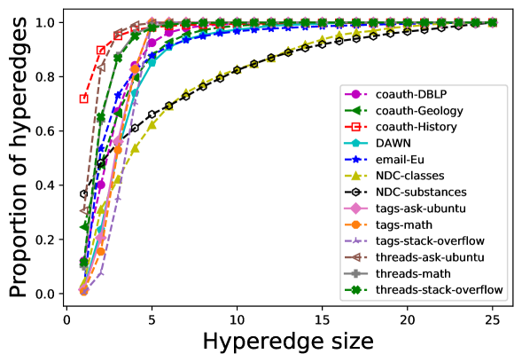
Figure 5. Cumulative distribution of hyperedge sizes.

Inputs : (1) distribution of hyperedge sizes $S$ (with max size $\bar{s}$),

(2) distribution of number of new hyperedges $NP$,

(3) number of nodes $n$

Output : synthetic hypergraph $G$

1 initialize $G$ with $\left\lfloor{\bar{s}}/{2}\right\rfloor$ disjoint hyperedges of size $2$, and compute the degree of all nodes in them

2 for $i\leftarrow 1$ to $n$ do

3       sample a number $k$ from $NP$.

4       for $j\leftarrow 1$ to $k$ do

5             sample a hyperedge size s from $S$

6             if $s=1$ then

7                   add the hyperedge $\{i\}$ to $G$

8            else

9                   choose $(s-1)$ nodes independently with probability proportional to their degrees

10                   add the hyperedge of $i$ and the $s-1$ nodes to $G$

11            

12      

13      for each node involved the $k$ newly formed hyperedges with $i$ do

14             increase the degree of each node by the number of its involving hyperedges

15      

Algorithm 2 NaivePA (Baseline Model)

Appendix B Appendix: Pseudocode

B.1. Pseudocode for NaivePA

Pseudocode for NaivePA is provided in Algorithm 2. Unlike HyperPA, which maintains the degree of every subset of every hyperedge, NaivePA only maintains the degree of individual nodes. When forming hyperedges with each newly arrived node, NaivePA chooses several nodes independently based on their degrees.

Inputs : (1) distribution of hyperedge sizes $S$,

(2) distribution of number of new hyperedges $NP$,

(3) number of nodes $n$,

(4) sampling rule $P$,

(5) probability $p$

Output : synthetic hypergraph $G$

1 initialize $G$ with $2$ disjoint hyperedges of maximum size in $S$

2 for $i\leftarrow 1$ to $n$ do

3       sample a number $k$ from $NP$

4       for $j\leftarrow 1$ to $k$ do

5             sample a size s from $S$

6             if $s=1$ then

7                   add the hyperedge $\{i\}$ to $G$

8            else

9                   initialize $B$ to $\{i\}$

10                   while $|B|<s$ do

11                         initialize $T$ to an empty set

12                         sample a hyperedge $E$ of $G$ based on $P$

13                         sample each node $v\in E$ into $B$ with prob. $p$

14                         if $|T|\leq s-|B|$ then

15                               $B\leftarrow B\cup T$

16                              

17                        else

18                               $T\leftarrow$ randomly chosen $s-|B|$ nodes in $T$

19                               $B\leftarrow B\cup T$

20                        

21                  add the hyperedge $B$ to $G$

22            

23      

Algorithm 3 Subset Sampling (Baseline Model)

B.2. Pseudocode for Subset Sampling

We present the pseudocode for Subset Sampling in Algorithm 3. For Subset Sampling, in order to keep the model simple, we tried the following variants for the sampling rule $P$:

• random: a hyperedge is randomly chosen among all previously formed hyperedges.

• recent: among all available hyperedges $E_{1},E_{2},...,E_{n}$, hyperedge $E_{i}$ has probability of being chosen equal to $\frac{i}{\sum_{j=1}^{n}j}$.

• $k$ most recent: only sample a set based on random or recent from the $k$ most recent hyperedges.

Empirical data shows that when $P$ is k most recent, the resulting graph has an unrealistically high diameter, while none between random and recent outperforms the other. For probability $p$, increasing from $0.4$ does not significantly change the result, while too low values make the graph shattered at the triangle-level decomposition. The reported results of Subset Sampling are from $p=0.8$ and $P=random$.

Appendix C Appendix: Proofs

C.1. Recovering hypergraphs from decomposed graphs

In this section, we prove that the original hypergraph can be recovered exactly from its decomposed graphs. To this end, we consider decomposed graphs with self-loops and edge weights, which are ignored in the previous sections since they do not contribute to the presented patterns. Specifically, for each $k$-level decomposed graph $G_{(k)}=(V_{(k)},E_{(k)})$ of a hypergraph $G=(V,E)$, we introduce a weight function $\omega_{(k)}$, defined as follows:

$$\omega_{(k)}\big{(}\{u_{(k)},v_{(k)}\}\big{)}:=|\{e\in E:u_{(k)}\cup v_{(k)}\subseteq e\}|.$$

That is, for each edge $\{u_{(k)},v_{(k)}\}$ in $E_{(k)}$, $\omega_{(k)}$ gives the number of hyperedges in $E$ that contain the union of $u_{(k)}$ and $v_{(k)}$. Additionally, for each hyperedge $\{a\}\in E$ of size $1$, we add a self-loop to the node $\{a\}$ in the $1$-level decomposed graph.

Theorem 1.

(Recovery of original hypergraphs). Assume that the maximum size of a hyperedge in a given hypergraph is $m$. If we have all the decomposed graphs up to level $(m-1)$ with edge weights and self-loops, we can recover the original hypergraph.

Proof.

Initialize an empty set $S=\emptyset$, which will contain the recovered hyperedges. We recover the hyperedges sized from the largest to smallest. By our definition, a hyperedge of size $n>k$ results in a clique of size ${n}\choose{k}$ in the $k$-level decomposed graph.

We start with the $(m-1)$-level decomposed graph: for each edge between two distinct $(m-1)$-level nodes $\{a_{1},...,a_{m-1}\}$ and $\{b_{1},...,b_{m-1}\}$, as $m$ is the maximum size for any hyperedge, the union of these two $(m-1)$-level nodes must be an original hyperedge $e$ of size $m$. We add this hyperedge $e$ into $S$ and decrement the weight of each edge involved in the resulting clique of $e$ in the $(m-1)$-level decomposed graph. We keep doing this until we completely clear the graph (i.e., making the weights of all edges to $0$) to recover all hyperedges of size $m$.

Assume that we have recovered all hyperedges of sizes greater than $k$ and have stored them in $S$. In the $(k-1)$-level decomposed graph, we decrement the weight of each edge involved in the clique resulting from each hyperedge currently in $S$. Then, we repeat the process above to recover all hyperedges of size $k$.

By continuing this procedure, eventually we can also recover all hyperedges of sizes at least $2$ after processing the node-level decomposed graph (i.e., $1$-level decomposed graph). Since we also maintain self-loops, we can recover all hyperedges of size $1$. The proof is completed here. ∎

C.2. Randomness in HyperPA

We present a simple proof about the randomness in HyperPA.

Theorem 2.

(Randomness in HyperPA). Given that the largest size $s$ possible in the distribution $S$ is a finite number $\bar{s}$, the conditional statement at line 8 of Algorithm 1, denoted as statement U, holds at most $\left\lfloor\frac{\bar{s}}{2}-1\right\rfloor$ times.

Proof.

Assume that at a given time step $t$, the sampled size at line 5 is $s$ and U holds. Then, the following conditions must be satisfied:

1. All $(s-1)$-sized groups have 0 degree, i.e., up to the time step $t$, only hyperedges of sizes up to $s-2$ present in the hypergraph,

2. $s\geq 4$,

where the second condition is from the first condition and the fact that the hypergraph is initialized with $12$ hyperedges of size $2$. Denote two consecutive time steps when U holds as $t$ and $t^{\prime}$, respectively. Denote the hyperedge sizes sampled at line 5 at time steps $t$ and $t^{\prime}$ as $s$ and $s^{\prime}$, respectively. According to the above two conditions, $s\geq 4$ and $s\leq s^{\prime}-2$. Assume U holds $M$ times at time steps $t_{1},..,t_{M}$, and denote the hyperedge sizes sampled at line 5 of the algorithm at these time steps as $s_{1},...,s_{M}$, respectively. Then, as shown,

$$s_{1}\leq s_{2}-2\leq s_{3}-4\leq...\leq s_{M}-2\times(M-1).$$

Then, $2\times(M-1)\leq s_{M}-s_{1}$. This, $s_{1}\geq 4$, and $s_{M}\leq\bar{s}$ imply $2\times(M-1)\leq\bar{s}-4$ or equivalently $M\leq\frac{\bar{s}}{2}-1$. As $M$ must be an integer, we conclude that $M\leq\left\lfloor\frac{\bar{s}}{2}-1\right\rfloor$. ∎

As in our datasets, the maximum hyperedge size is 25 and the distribution $S$ used for HyperPA is learned from the dataset, we have $\bar{s}=25$ for HyperPA. According to the proof, the conditional statement at line 8 of Algorithm 1 can only hold at most 11 times. If the number of nodes $n$ is relatively large, most of the time when $s>1$, the conditional statement at line 8 in Algorithm 1 does not hold, indicating that lines 12-13 of the pseudocode are executed.

References

- (1)
- app (2020) 2020. Supplementary results, code and datasets. Available online: https://github.com/manhtuando97/KDD-20-Hypergraph.
- Abello et al. (1998) James Abello, Adam L Buchsbaum, and Jeffery R Westbrook. 1998. A functional approach to external graph algorithms. In ESA.
- Abello et al. (2013) James Abello, Panos M Pardalos, and Mauricio GC Resende. 2013. Handbook of massive data sets. Vol. 4. Springer.
- Akoglu et al. (2008) Leman Akoglu, Mary McGlohon, and Christos Faloutsos. 2008. RTM: Laws and a recursive generator for weighted time-evolving graphs. In ICDM.
- Akoglu et al. (2010) Leman Akoglu, Mary McGlohon, and Christos Faloutsos. 2010. Oddball: Spotting anomalies in weighted graphs. In PAKDD.
- Albert et al. (1999) Réka Albert, Hawoong Jeong, and Albert-László Barabási. 1999. Internet: Diameter of the world-wide web. Nature 401, 6749 (1999), 130.
- Albert et al. (2002) Réka Albert, Hawoong Jeong, and Albert-László Barabási. 2002. Statistical mechanics of complex networks. Rev. Mod. Phys (2002).
- Alstott and Bullmore (2014) Jeff Alstott and Dietmar Plenz Bullmore. 2014. powerlaw: a Python package for analysis of heavy-tailed distributions. PloS one 9, 1 (2014).
- Barabási and Albert (1999) Albert-László Barabási and Réka Albert. 1999. Emergence of scaling in random networks. Science 286, 5439 (1999), 509–512.
- Benson et al. (2018a) Austin R Benson, Rediet Abebe, Michael T Schaub, Ali Jadbabaie, and Jon Kleinberg. 2018a. Simplicial closure and higher-order link prediction. Proc. Natl. Acad. Sci. U.S.A 115, 48 (2018), E11221–E11230.
- Benson et al. (2016) Austin R Benson, David F Gleich, and Jure Leskovec. 2016. Higher-order organization of complex networks. Science 353, 6295 (2016), 163–166.
- Benson et al. (2018b) Austin R Benson, Ravi Kumar, and Andrew Tomkins. 2018b. Sequences of sets. In KDD.
- Bollobás and Riordan (2004) Béla Bollobás and Oliver Riordan. 2004. The diameter of a scale-free random graph. Combinatorica 24, 1 (2004), 5–34.
- Bonacich et al. (2004) Phillip Bonacich, Annie Cody Holdren, and Michael Johnston. 2004. Hyper-edges and multi-dimensional centrality. Soc. Netw 26, 3 (2004), 189–203.
- Broder et al. (2000) Andrei Broder, Ravi Kumar, Farzin Maghoul, Prabhakar Raghavan, Sridhar Rajagopalan, Raymie Stata, Andrew Tomkins, and Janet Wiener. 2000. Graph structure in the web. Computer networks 33, 1-6 (2000), 309–320.
- C (2013) Berge C. 2013. Hypergraphs. Vol. 45. North Holland, Amsterdam.
- Chodrow (2019) Philip S Chodrow. 2019. Configuration Models of Random Hypergraphs and their Applications. arXiv preprint arXiv:1902.09302 (2019).
- Chung and Lu (2002) Fan Chung and Linyuan Lu. 2002. The average distances in random graphs with given expected degrees. Proc. Natl. Acad. Sci. U.S.A 99, 25 (2002), 15879–15882.
- Clauset et al. (2009) Aaron Clauset, Cosma Rohilla Shalizi, and Mark EJ Newman. 2009. Power-law distributions in empirical data. SIAM review 51, 4 (2009), 661–703.
- Cooper and Frieze (2003) Colin Cooper and Alan Frieze. 2003. A general model of web graphs. Random Struct. Algorithms 22, 3 (2003), 311–335.
- Easley et al. (2010) David Easley, Jon Kleinberg, et al. 2010. Networks, crowds, and markets. Vol. 8. Cambridge university press Cambridge.
- Edunov et al. (2016) Sergey Edunov, Dionysios Logothetis, Cheng Wang, Avery Ching, and Maja Kabiljo. 2016. Darwini: Generating realistic large-scale social graphs. arXiv:1610.00664 (2016).
- Eikmeier and Gleich (2017) Nicole Eikmeier and David F Gleich. 2017. Revisiting power-law distributions in spectra of real world networks. In KDD.
- Faloutsos et al. (1999) Michalis Faloutsos, Petros Faloutsos, and Christos Faloutsos. 1999. On power-law relationships of the internet topology. In ACM SIGCOMM computer communication review, Vol. 29. ACM, 251–262.
- Girvan and Newman (2002) M. Girvan and M. E. J. Newman. 2002. Community structure in social and biological networks. Proc. Natl. Acad. Sci. U.S.A 99 (2002).
- Kang et al. (2010) U Kang, Mary McGlohon, Leman Akoglu, and Christos Faloutsos. 2010. Patterns on the Connected Components of TerabyteScale Graphs. In ICDM.
- Kleinberg (2002) Jon M Kleinberg. 2002. Small-world phenomena and the dynamics of information. In NIPS.
- Kleinberg et al. (1999) Jon M Kleinberg, Ravi Kumar, Prabhakar Raghavan, Sridhar Rajagopalan, and Andrew S Tomkins. 1999. The web as a graph: measurements, models, and methods. In COCOON.
- Kolda et al. (2014) Tamara G Kolda, Ali Pinar, Todd Plantenga, and Comandur Seshadhri. 2014. A scalable generative graph model with community structure. SIAM J. Sci. Comput 36, 5 (2014), C424–C452.
- Kumar et al. (2000) R. Kumar, P. Raghavan, S. Rajagopalan, D. Sivakumar, A. Tomkins, and E. Uptal. 2000. Stochastic models for the web graph. In FOCS.
- Leskovec et al. (2008) Jure Leskovec, Lars Backstrom, Ravi Kumar, and Andrew Tomkins. 2008. Microscopic evolution of social networks. In KDD.
- Leskovec et al. (2010) Jure Leskovec, Deepayan Chakrabarti, Jon Kleinberg, Christos Faloutsos, and Zoubin Ghahramani. 2010. Kronecker Graphs: An Approach to Modeling Networks. J. Mach. Learn. Res 11 (2010), 985–1042.
- Leskovec et al. (2005) Jure Leskovec, Jon Kleinberg, and Christos Faloutsos. 2005. Graphs over time: densification laws, shrinking diameters and possible explanations. In KDD.
- Lilliefors (1969) Hubert W Lilliefors. 1969. On the Kolmogorov-Smirnov test for the exponential distribution with mean unknown. J. Amer. Statist. Assoc. 64 (1969), 387–389.
- Liu et al. (2019) Paul Liu, Austin Benson, and Moses Charikar. 2019. A sampling framework for counting temporal motifs. In WSDM.
- Mahadevan et al. (2006) Priya Mahadevan, Dmitri Krioukov, Kevin Fall, and Amin Vahdat. 2006. Systematic topology analysis and generation using degree correlations. In SIGCOMM.
- Milgram (1967) Stanley Milgram. 1967. The small-world problem. Psychology Today 2, 1 (1967), 60–67.
- Milo et al. (2002) Ron Milo, Shai Shen-Orr, Shalev Itzkovitz, Nadav Kashtan, Dmitri Chklovskii, and Uri Alon. 2002. Network motifs: simple building blocks of complex networks. Science 298, 5594 (2002), 824–827.
- Mitzenmacher (2004) Michael Mitzenmacher. 2004. A brief history of generative models for power law and lognormal distributions. Internet Mathematics 1, 2 (2004), 226–251.
- Newman (2001) Mark EJ Newman. 2001. Clustering and preferential attachment in growing networks. Physical review E 64, 2 (2001), 025102.
- Paranjape et al. (2017) Ashwin Paranjape, Austin R Benson, and Jure Leskovec. 2017. Motifs in temporal networks. In WSDM.
- Sala et al. (2010) Alessandra Sala, Lili Cao, Christo Wilson, Robert Zablit, Haitao Zheng, and Ben Y Zhao. 2010. Measurement-calibrated graph models for social network experiments. In WWW.
- Shin (2017) Kijung Shin. 2017. Wrs: Waiting room sampling for accurate triangle counting in real graph streams. In ICDM.
- Shin et al. (2018) Kijung Shin, Tina Eliassi-Rad, and Christos Faloutsos. 2018. Patterns and anomalies in k-cores of real-world graphs with applications. Knowl. Inf. Syst 54, 3 (2018), 677–710.
- Sinha et al. (2015) Arnab Sinha, Zhihong Shen, Yang Song, Hao Ma, Darrin Eide, Bo-June (Paul) Hsu, and Kuansan Wang. 2015. An Overview of Microsoft Academic Service (MAS) and Applications. In WWW.
- Stasi et al. (2014) Despina Stasi, Kayvan Sadeghi, Alessandro Rinaldo, Sonja Petrović, and Stephen E Fienberg. 2014. models for random hypergraphs with a given degree sequence. arXiv preprint arXiv:1407.1004 (2014).
- Vázquez (2003) Alexei Vázquez. 2003. Growing network with local rules: Preferential attachment, clustering hierarchy, and degree correlations. Physical Review E 67, 5 (2003), 056104.
- Watts and Strogatz (1998) Duncan J Watts and Steven H Strogatz. 1998. Collective dynamics of ‘small-world’networks. Nature 393, 6684 (1998), 440.
- Xu et al. (2013) Ye Xu, Dan Rockmore, and Adam M Kleinbaum. 2013. Hyperlink prediction in hypernetworks using latent social features. In DS.
- Yin et al. (2017) Hao Yin, Austin R Benson, Jure Leskovec, and David F Gleich. 2017. Local higher-order graph clustering. In KDD.
- Yoon et al. (2020) Se-eun Yoon, Hyungseok Song, Kijung Shin, and Yung Yi. 2020. How Much and When Do We Need Higher-order Information in Hypergraphs? A Case Study on Hyperedge Prediction. In WWW.
- Zhou et al. (2006) Dengyong Zhou, Jiayuan Huang, and Bernhard Scholkopf. 2006. Learning with Hypergraphs: Clustering, Classification, and Embedding. In NIPS.