Abstract

We propose kernel distributionally robust optimization (Kernel DRO) using insights from the robust optimization theory and functional analysis. Our method uses reproducing kernel Hilbert spaces (RKHS) to construct a wide range of convex ambiguity sets, which can be generalized to sets based on integral probability metrics and finite-order moment bounds. This perspective unifies multiple existing robust and stochastic optimization methods. We prove a theorem that generalizes the classical duality in the mathematical problem of moments. Enabled by this theorem, we reformulate the maximization with respect to measures in DRO into the dual program that searches for RKHS functions. Using universal RKHSs, the theorem applies to a broad class of loss functions, lifting common limitations such as polynomial losses and knowledge of the Lipschitz constant. We then establish a connection between DRO and stochastic optimization with expectation constraints. Finally, we propose practical algorithms based on both batch convex solvers and stochastic functional gradient, which apply to general optimization and machine learning tasks.

1 INTRODUCTION

Imagine a hypothetical scenario in the illustrative figure where we want to arrive at a destination while avoiding unknown obstacles. A worst-case robust optimization (RO) Ben-Tal et al. (2009) approach is then to avoid the entire unsafe area (left, blue). Suppose we have historical locations of the obstacles (right, dots). We may choose to avoid only the convex polytope that contains all the samples (pink). This data-driven robust decision-making idea improves efficiency while retaining robustness.

The concept of distributional ambiguity concerns the uncertainty of uncertainty — the underlying probability measure is only partially known or subject to change. This idea is by no means a new one. The classical moment problem concerns itself with estimating the worst-case risk expressed by $\max_{P\in\mathcal{K}}{\int l\,dP}$ where $l$ is some loss function. The constraint $P\in\mathcal{K}$ describes the distribution ambiguity, i.e., $P$ is only known to live within a subset $\mathcal{K}$ of probability measures. The solution to the moment problem gives the risk under some worst-case distribution within $\mathcal{K}$. To make decisions that will minimize this worst-case risk is the idea of distributionally robust optimization (DRO) Delage and Ye (2010), Scarf (1958).

Many of today’s learning tasks suffer from various manifestations of distributional ambiguity — e.g., covariate shift, adversarial attacks, simulation to reality transfer — phenomena that are caused by the discrepancy between training and test distributions. Kernel methods are known to possess robustness properties, e.g., Christmann and Steinwart (2007), Xu et al. (2009). However, this robustness only applies to kernelized models. This paper extends the robustness of kernel methods using the robust counterpart formulation techniques Ben-Tal et al. (2009) as well as the principled conic duality theory Shapiro (2001). We term our approach kernel distributionally robust optimization (Kernel DRO), which can robustify general optimization solutions not limited to kernelized models.

The main contributions of this paper are:

1. We rigorously prove the generalized duality theorem (Theorem 3.1) that reformulates general DRO into a convex dual problem searching for RKHS functions, lifting common limitations of DRO on the loss functions, such as the knowledge of Lipschitz constant. The theorem also constitutes a generalization of the duality results from the literature of mathematical problem of moments.

2. We use RKHSs to construct a wide range of convex ambiguity sets (in Table 1, 3), including sets based on integral probability metrics (IPM) and finite-order moment bounds. This perspective unifies existing RO and DRO methods.

3. We propose computational algorithms based on both convex solvers and stochastic approximation, which can be applied to robustify general optimization and machine learning models not limited to kernelized or known-Lipschitz-constant ones.

4. Finally, we establish an explicit connection between DRO and stochastic optimization with expectation constraints. This leads to a novel stochastic functional gradient DRO (SFG-DRO) algorithm which can scale up to modern machine learning tasks.

In addition, we give complete self-contained proofs in the appendix that shed light on the connection between RKHSs, conic duality, and DRO. We also show that universal RKHSs are large enough for DRO from the perspective of functional analysis through concrete examples.

2 BACKGROUND

Notation.

$\mathcal{X}\subset\mathbb{R}^{d}$ denotes the input domain, which is assumed to be compact unless otherwise specified. $\mathcal{P}:=\mathcal{P}(\mathcal{X})$ denotes the set of all Borel probability measures on $\mathcal{X}$. We use ${\hat{P}}$ to denote the empirical distribution ${\hat{P}}=\sum_{i=1}^{N}{\frac{1}{N}}\delta_{\xi_{i}}$, where $\delta$ is a Dirac measure and $\{\xi_{i}\}_{i=1}^{N}$ are data samples. We refer to the function $\delta_{\mathcal{C}}(x):=0$ if $x\in\mathcal{C}$, $\infty$ if $x\notin\mathcal{C}$, as the indicator function. $\delta^{*}_{\mathcal{C}}(f):=\sup_{\mu\in\mathcal{C}}\langle{f,\mu}\rangle_{\mathcal{H}}$ is the support function of $\mathcal{C}$. $S_{N}$ denotes the $N$-dimensional simplex. $\mathrm{ri}(\cdot)$ denotes the relative interior of a set. A function $f$ is upper semicontinuous on $\mathcal{X}$ if $\limsup_{x\to x_{0}}f(x)\leq f(x_{0}),\forall x_{0}\in\mathcal{X}$; it is proper if it is not identically $-\infty$. When there is no ambiguity, we simplify the loss function notation $l(\theta,\cdot)$ by using $l$ to indicate that results hold for $\theta$ point-wise.

2.1 Robust and distributionally robust optimization

Robust optimization (RO) Ben-Tal et al. (2009) studies mathematical decision-making under uncertainty. It solves the min-max problem (omitting constraints) $\ \min_{\theta}\sup_{\xi\in\mathcal{X}}l(\theta,\xi),$ where $l(\theta,\xi)$ denotes a general loss function, $\theta$ is the decision variable, and $\xi$ is a variable representing the uncertainty. Intuitively, RO makes the decision assuming an adversarial scenario, as reflected in taking supremum w.r.t. $\xi$. For this reason, it is often referred to as the worst-case RO. Recently, RO has been applied to the setting of adversarially robust learning, e.g., in Madry et al. (2019), Wong and Kolter (2018), which we will visit in this paper. In the optimization literature, a typical approach to solving RO is via reformulating the min-max program using duality to obtain a single minimization problem. In contrast, distributionally robust optimization (DRO) minimizes the expected loss assuming the worst-case distribution:

$$\min_{\theta}\underset{P\in\mathcal{K}}{\sup}\bigg{\{}\int l(\theta,\xi)\ dP(\xi)\bigg{\}},$$ (1)

where $\mathcal{K}\subseteq\mathcal{P}$, called the ambiguity set, is a subset of distributions, e.g., all distributions with the given mean and variance. Compared with RO, DRO only robustifies the solution against a subset $\mathcal{K}$ of distributions on $\mathcal{X}$ and is, therefore, less conservative (since $\sup_{P\in\mathcal{K}}\{\int l(\theta,\xi)\ dP(\xi)\}\leq\sup_{\xi\in\mathcal{X}}l(\theta,\xi)$).

The inner problem of (1), historically known as the problem of moments traced back at least to Thomas Joannes Stieltjes, estimates the worst-case risk under uncertainty in distributions. The modern approaches, pioneered by the work of Isii (1962) (see also Lasserre (2002), Shapiro (2001), Bertsimas and Popescu (2005), Popescu (2005), Vandenberghe et al. (2007), Van Parys et al. (2016), Zhu et al. (2020)), typically seek a sharp upper bound via duality. This duality, rigorously justified in Shapiro (2001), is different from that in the Euclidean space because infinite-dimensional convex sets can become pathological. Using that methodology, we can reformulate DRO (1) into a single solvable minimization problem.

Existing DRO approaches can be grouped into three main categories by the type of ambiguity sets used. DRO with (finite-order) moment constraints has been studied in Delage and Ye (2010), Scarf (1958), Zymler et al. (2013). The authors of Ben-Tal et al. (2013), Iyengar (2005), Nilim and El Ghaoui (2005), Wang et al. (2016), Duchi et al. (2016) studied DRO using likelihood bounds as well as $\phi-$divergence. Wasserstein-distance-based DRO has been studied by the authors of Mohajerin Esfahani and Kuhn (2018), Zhao and Guan (2018), Gao and Kleywegt (2016), Blanchet et al. (2019), and applied in a large body of literature. Many existing approaches require either the assumptions such as quadratic loss functions or the knowledge of Lipschitz constant or RKHS norm of the loss $l$, which are often hard to obtain in practice; see Virmaux and Scaman (2018), Bietti et al. (2019).

2.2 Reproducing kernel Hilbert spaces

A symmetric function $k\colon\mathcal{X}\times\mathcal{X}\to\mathbb{R}$ is called a positive definite kernel if $\sum_{i=1}^{n}\sum_{i=1}^{n}a_{i}a_{j}k(x_{i},x_{j})\geq 0$ for any $n\in\mathbb{N}$, $\{x_{i}\}_{i=1}^{n}\subset\mathcal{X}$, and $\{a_{i}\}_{i=1}^{n}\subset\mathbb{R}$. Given a positive definite kernel $k$, there exists a Hilbert space $\mathcal{H}$ and a feature map $\phi\colon\mathcal{X}\to\mathcal{H}$, for which $k(x,y)=\langle\phi(x),\phi(y)\rangle_{\mathcal{H}}$ defines an inner product on $\mathcal{H}$, where $\mathcal{H}$ is a space of real-valued functions on $\mathcal{X}$. The space $\mathcal{H}$ is called a reproducing kernel Hilbert space (RKHS). It is equipped with the reproducing property: $f(x)=\langle f,\phi(x)\rangle_{\mathcal{H}}$ for any $f\in\mathcal{H},x\in\mathcal{X}$. By convention, we will denote the canonical feature map as $\phi(x):=k(x,\cdot)$. Properties of the functions in $\mathcal{H}$ are inherited from the properties of $k$. For instance, if $k$ is continuous, then any $f\in\mathcal{H}$ is continuous. A continuous kernel $k$ on a compact metric space $\mathcal{X}$ is said to be universal if $\mathcal{H}$ is dense in $C(\mathcal{X})$ (Steinwart and Christmann, 2008, Section 4.5). A universal $\mathcal{H}$ can thus be considered a large RKHS since any continuous function can be approximated arbitrarily well by a function in $\mathcal{H}$. An example of a universal kernel is the Gaussian kernel $k(x,y)=\exp\left(-\frac{\|x-y\|^{2}_{2}}{2\sigma^{2}}\right)$ defined on $\mathcal{X}$ where $\sigma>0$ is the bandwidth parameter.

RKHSs first gained widespread attention following the advent of the kernelized support vector machine (SVM) for classification problems Cortes and Vapnik (1995), Boser et al. (1992), Schölkopf et al. (2000). More recently, the use of RKHSs has been extended to manipulating and comparing probability distributions via kernel mean embedding Smola et al. (2007). Given a distribution $P$, and a (positive definite) kernel $k$, the kernel mean embedding of $P$ is defined as $\mu_{P}:=\int k(x,\cdot)\,dP$. If $\mathbb{E}_{x\sim P}[k(x,x)]<\infty$, then $\mu_{P}\in\mathcal{H}$ (Smola et al., 2007, Section 1.2). The reproducing property allows one to easily compute the expectation of any function $f\in\mathcal{H}$ since $\mathbb{E}_{x\sim P}[f(x)]=\langle f,\mu_{P}\rangle_{\mathcal{H}}$. Embedding distributions into $\mathcal{H}$ also allows one to measure the distance between distributions in $\mathcal{H}$. If $k$ is universal, then the mean map $P\mapsto\mu_{P}$ is injective on $\mathcal{P}$ Gretton et al. (2012). With a universal $\mathcal{H}$, given two distributions $P,Q$, $\|\mu_{P}-\mu_{Q}\|_{\mathcal{H}}$ defines a metric. This quantity is known as the maximum mean discrepancy (MMD) Gretton et al. (2012). With $\|f\|_{\mathcal{H}}:=\sqrt{\langle f,f\rangle_{\mathcal{H}}}$ and the reproducing property, it can be shown that $\|\mu_{P}-\mu_{Q}\|_{\mathcal{H}}^{2}=\mathbb{E}_{x,x^{\prime}\sim P}k(x,x^{\prime})+\mathbb{E}_{y,y^{\prime}\sim Q}k(y,y^{\prime})-2\mathbb{E}_{x\sim P,y\sim Q}k(x,y)$, allowing the plug-in estimator to be used for estimating the MMD from empirical data. The MMD is an instance of the class of integral probability metrics (IPMs), and can equivalently be written as $\|\mu_{P}-\mu_{Q}\|_{\mathcal{H}}=\sup_{\|f\|_{\mathcal{H}}\leq 1}\int f\,d(P-Q)$, where the optimum $f^{*}$ is a witness function Gretton et al. (2012), Sriperumbudur et al. (2012).

3 THEORY

We make the following assumption for the proof.

Assumption 3.1.

$l(\theta,\cdot)$ is proper, upper semicontinuous. $\mathcal{C}$ is closed convex. $\mathrm{ri}(\mathcal{K}_{\mathcal{C}})\neq\emptyset$.

This assumption is general in that it does not require the knowledge of the Lipschitz constant or the RKHS $l(\theta,\cdot)$ lives in. Generally speaking, the DRO problem (1) requires two essential elements: an appropriate ambiguity set that contains meaningful distributions and a sharp reformulation of the min-max problem. We first present the former in Section 3.1, and then the latter in Section 3.2. Complete proofs of our theory are deferred to the appendix.

3.1 Generalized primal formulation

We now present the primal formulation of kernel distributionally robust optimization (Kernel DRO) as a generalization of existing DRO frameworks.

$$(P):=\min_{\theta}\underset{P,\mu}{\sup}\bigg{\{}{\int l(\theta,\xi)\ dP(\xi)}\colon\\ {\int{\phi}{\ dP}=\mu,P\in\mathcal{P},\mu\in\mathcal{C}}\bigg{\}},$$ (2)

where $\mathcal{H}$ is an RKHS whose feature map is $\phi$. Both sides of the constraint $\int{\phi}{\ dP}=\mu$ are functions in $\mathcal{H}$. Note $\mu$ can be viewed as a generalized moment vector, which is constrained to lie within the set $\mathcal{C}\subseteq\mathcal{H}$, referred to as an (RKHS) ambiguity set. Let us denote the set of all feasible distributions in (2) as $\mathcal{K}_{\mathcal{C}}={\{P\colon\int\phi\ dP=\mu,\mu\in\mathcal{C},P\in\mathcal{P}\}}$, i.e., $\mathcal{K}_{\mathcal{C}}$ is the usual ambiguity set. Intuitively, the set $\mathcal{C}$ restricts the RKHS embeddings of distributions in the ambiguity set $\mathcal{K}_{\mathcal{C}}$. In this paper, we take a geometric perspective to construct $\mathcal{C}$ using convex sets in $\mathcal{H}$. Given data samples $\{\xi_{i}\}_{i=1}^{N}$, we outline various choices for $\mathcal{C}$ in the left column of Table 1 (and 3 in the appendix), and illustrate our intuition in Figure 1.

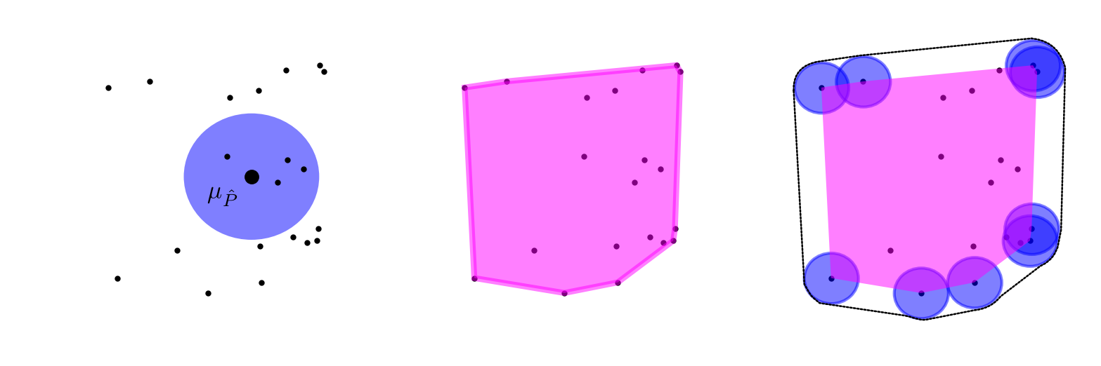
(a) RKHS ambiguity sets $\mathcal{C}$

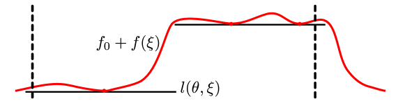
(b) Interpretation of Kernel DRO

Figure 1: (a): Geometric intuition for choosing ambiguity set $\mathcal{C}$ in $\mathcal{H}$ such as norm-ball, polytope, and Minkowski sum of sets. The scattered points are the embeddings of empirical samples. See Table 3 for more examples. (b): Geometric interpretation of Kernel DRO (4). The (red) curve depicts $f_{0}+f$, which majorizes $l(\theta,\cdot)$ (black). The horizontal axis is $\xi$. The dashed lines denote the boundary of the domain $\mathcal{X}$.

Table 1: Examples of support functions for Kernel DRO. See Table 3 for more details.

RKHS ambiguity set $\mathcal{C}$	Support function $\delta^{*}_{\mathcal{C}}(f)$
RKHS norm-ball $\mathcal{C}=\{\mu\colon\|\mu-\mu_{\hat{P}}\|_{\mathcal{H}}\leq\epsilon\}$	${\frac{1}{N}\sum_{i=1}^{N}f(\xi_{i})+\epsilon\|{f}\|_{\mathcal{H}}}$
Polytope $\mathcal{C}=\mathrm{conv}\{\phi(\xi_{1}),\dots,\phi(\xi_{N})\}$	${\max_{i}f(\xi_{i})}$ (scenario optimization; SVMs with no slack)
Minkowski sum $\mathcal{C}=\sum_{i=1}^{N}\mathcal{C}_{i}$	${\sum_{i=1}^{N}\delta^{*}_{\mathcal{C}_{i}}(f)}$
Whole space $\mathcal{C}=\mathcal{H}$	$0$ if $f=0$, $\infty$ otherwise (worst-case RO Ben-Tal et al. (2009))

To better understand our unifying formulation, let us examine the celebrated SVM through the lens of our generalized formulation.

Example 3.1 (SVM as generalized DRO).

Let us consider SVM for regression, without using slack variables or regularization for simplicity. This can be formulated as optimizing the loss $\min_{f\in\mathcal{H}}\max_{i}[|y_{i}-f(x_{i})|-\eta]_{+}$ where $\eta>0$ is the parameter for the hinge loss. This can be seen as the generalized DRO

$$\min_{f\in\mathcal{H}}\sup_{P\in\mathcal{K}}\int[|y-f(x)|-\eta]_{+}dP(x,y),$$

where the ambiguity set is given by the polytope $\mathcal{K}=\mathrm{cl}\mathrm{conv}\{\delta_{\xi_{1}},\dots,\delta_{\xi_{N}}\},\xi_{i}=(x_{i},y_{i})$.

Let us now consider a small RKHS to understand the effect of different RKHSs on Kernel DRO.

Example 3.2 (DRO with non-universal kernels).

Consider distributions $\hat{P}=\mathcal{N}(0,1),Q_{v}=\mathcal{N}(0,v^{2})$ and $\mathcal{H}_{1}$ induced by the linear kernel $k_{1}(x,y):=xy$. $\mathcal{H}_{1}$ is small since it only contains linear functions. $\mathrm{MMD}_{k_{1}}(\hat{P},Q_{v})=0,\forall v\neq 0$ since they share the first moment. Therefore, any $\mathcal{C}$ that contains $\mu_{\hat{P}}$ also contains all the distributions in $\{\mu_{Q_{v}},v\neq 0\}$.

This example shows that small RKHSs force Kernel DRO to robustify against a large set of distributions, resulting in conservativeness. In the extreme, if we choose the smallest possible RKHS $\mathcal{H}=\{0\}$, then the space does not contain functions to separate any distinct distributions. This renders Kernel DRO (4) overly conservative since we can only choose $f=0$ in (4) — it is precisely reduced to worst-case RO. On the other extreme, the next example shows the downside of function spaces that are too large.

Example 3.3 (DRO with large function space).

Suppose $\mathcal{H}$ is the space of all bounded measurable functions, the metric induced by $\mathcal{H}$ becomes the total variation distance Sriperumbudur et al. (2011). While the induced topology is strong, (4) has a trivial solution $f=l,f_{0}=0$. By plugging this solution into (4), we recover (2). Hence the reformulation becomes meaningless.

We distinguish between DRO without metrics, e.g., moment constraints and SVMs, and DRO with probability metric or divergence, e.g., Wasserstein metric. Let us first examine an instance of the former using Kernel DRO. We return to the latter at the end of this section.

Example 3.4 (Reduction to DRO with moment constraints).

Kernel DRO with the second-order polynomial kernel $k_{2}(x,y):=(1+x^{\top}y)^{2}$ and a singleton ambiguity set $\mathcal{C}=\{\mu_{\hat{P}}\}$ robustifies against all distributions sharing the first two moments with $\hat{P}$. This is equivalent to DRO with known first two moments, such as in Delage and Ye (2010), Scarf (1958). More generally, the choice of the $p$th-order polynomial kernel $k_{p}(x,y):=(1+x^{\top}y)^{p}$ corresponds to DRO with known first $p$ moments.

If $\mathcal{H}$ is associated with a universal kernel (e.g., Gaussian), it is large since $\mathcal{H}$ is dense in the space of continuous functions (cf. Sriperumbudur et al. (2011)). Then the induced topology (MMD) is strong enough to separate distinct probability measures. Meanwhile, RKHS allows for efficient computation using tools from kernel methods, as shown in Section 4. Therefore, our insight is that universal RKHSs are large enough for DRO applications.

Remark.

For the RKHS associated with the Gaussian kernel, the diameter of the space can be computed: $\forall p,q,\|\mu_{p}-\mu_{q}\|_{\mathcal{H}}\leq\|\mu_{p}\|_{\mathcal{H}}+\|\mu_{q}\|_{\mathcal{H}}\leq 2\sup_{x,y}\sqrt{k(x,y)}=2$. Hence, if $\epsilon\geq 2$, $\mathcal{C}$ contains all probability distributions. Then, Kernel DRO is again reduced to worst-case RO on domain $\mathcal{X}$.

We now turn to DRO with a generalized class of integral probability metrics (IPM).

Example 3.5 (Generalization to IPM-DRO).

Suppose $d_{\mathcal{F}}(P,\hat{P}):=\sup_{f\in\mathcal{F}}\int fd(P-\hat{P})$ is the IPM defined by some function class $\mathcal{F}$. The IPM-DRO primal formulation is given by

$$\min_{\theta}\sup_{d_{\mathcal{F}}{(P,\hat{P})}\leq\epsilon}\int l(\theta,\xi)\ dP(\xi).$$ (3)

If we choose the class $\mathcal{F}=\{f:\|{f}\|_{\mathcal{H}}\leq 1\}$, we recover Kernel DRO with the RKHS norm-ball set in Table 1. Similarly, $\mathcal{F}=\{f:\mathrm{lip}{(f)}\leq 1\}$ recovers the (type-1) Wasserstein-DRO. This puts Wasserstein-DRO and Kernel DRO into a unified perspective.

3.2 Generalized duality theorem

We now present the main theorem of this paper, the generalized duality theorem of Kernel DRO (2).

Theorem 3.1 (Generalized Duality).

Under Assumption 3.1, (2) is equivalent to

$$(D):= \min_{\theta,f_{0}\in\mathbb{R},f\in\mathcal{H}} {\ f_{0}+\delta^{*}_{\mathcal{C}}(f)}$$ (4)

$$\operatorname*{\mathrm{subject}\ \mathrm{to}} l(\theta,\xi)\leq f_{0}+f(\xi),\ \forall\xi\in\mathcal{X}$$

where $\delta^{*}_{\mathcal{C}}(f):=\sup_{\mu\in\mathcal{C}}\langle{f,\mu}\rangle_{\mathcal{H}}$ is the support function of $\mathcal{C}$, i.e., $(P)=(D)$, strong duality holds for the inner moment problem for any $\theta$ point-wise.

The theorem holds regardless of the dependency of $l$ on $\theta$, e.g., non-convexity. If $l$ is convex in $\theta$, then (4) is a convex program. Formulation (4) has a clear geometric interpretation: we find a function $f_{0}+f$ that majorizes $l(\theta,\cdot)$ and subsequently minimize a surrogate loss involving $f_{0}$ and $f$. This is illustrated in Figure 1b. Note the term duality here refers to the inner moment problem. The statement can be further simplified by replacing $f_{0}+f$ with $f$. However, we choose the current notation for the sake of its explicit connection to RO.

Proof sketch.

Our weak duality proof follows standard paradigms of Lagrangian relaxation by introduing dual variables. Notably, we associate the functional constraint $\int{\phi}{\ dP}=\mu$ with a dual function $f\in\mathcal{H}$, which is the decision variable in the dual problem (4). Using the reproducing property of RKHSs and conic duality, we arrive at (4) with weak duality. Our strong duality proof is an extension of the conic strong duality in Eulidean spaces. We rely on the existance of separating hyperplnes between convex sets in locally convex function spaces, e.g., $\mathcal{H}$. See the illustration in Figure 2. In our generalized duality theorem, this separating hyperplane is determined by the witness function $f^{*}$, which is the optimal dual variable in (4). See the appendix for the full proof.

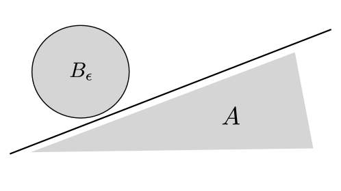
Figure 2: Illustration of a separating hyperplane in $\mathcal{H}$

Theorem 3.1 generalizes the classical bounds in generalized moment problems Isii (1962), Lasserre (2002), Shapiro (2001), Bertsimas and Popescu (2005), Popescu (2005), Vandenberghe et al. (2007), Van Parys et al. (2016) to infinitely many moments using RKHSs. A distinction between Theorem 3.1 and other DRO approaches is that it uses the density of universal RKHSs to find a surrogate which can sharply bound the worst-case risk. This means that we do not require the loss $l(\theta,\cdot)$ to be affine, quadratic, or living in a known RKHS, nor do we require the knowledge of Lipschitz constant or RKHS norm of $l(\theta,\cdot)$. To our knowledge, existing works typically require one of such assumptions.

Moreover, Theorem 3.1 generalizes existing RO and DRO in the sense that it gives us a unifying tool to work with various ambiguity and ambiguity sets, which may be customized for specific applications. We outline a few closed-form expressions of the support function $\delta^{*}_{\mathcal{C}}(f)$ in Table 1, and more in Table 3. We now return IPM-DRO with a duality result.

Corollary 3.1.1 (IPM-DRO duality).

Given the integral probability metric $d_{\mathcal{F}}(P,\hat{P}):=\sup_{f\in\mathcal{F}}\int fd(P-\hat{P})$, a dual program to (3) is given by

$$\min_{\theta,\lambda\geq 0,f_{0}\in\mathbb{R},f\in\mathcal{F}} \ {f_{0}+\frac{1}{N}\sum_{i=1}^{N}\lambda f(\xi_{i})+\lambda\epsilon}$$ (5)

$$\operatorname*{\mathrm{subject}\ \mathrm{to}} \ l(\theta,\xi)\leq f_{0}+\lambda f(\xi),\ \forall\xi\in\mathcal{X}.$$

The reduction to (4) as a special case can be seen by replacing $\lambda f$ with $f$ and choosing $\mathcal{F}=\mathcal{H}$.

We now establish an explicit connection between DRO and stochastic optimization with expectation constraint, whose solution methods using stochastic approximation are an topic of active research Lan and Zhou (2020), Xu (2020).

Corollary 3.1.2.

(Stochastic optimization with expectation constraint) Under the Assumption 3.1, the optimal value of (2) coincides with that of

$$\min_{\theta,f_{0}\in\mathbb{R},f\in\mathcal{H}} \ f_{0}+\delta^{*}_{\mathcal{C}}(f)$$ (6)

$$\operatorname*{\mathrm{subject}\ \mathrm{to}} \ \mathbb{E}h\left(l\left(\theta,\zeta\right)-f_{0}-\lambda f\left(\zeta\right)\right)\leq 0$$

for some function $h$ that satisfies $h(t)=0\text{ if }t\leq 0,h(t)>0\text{ if }t>0$, and random variable $\zeta\sim\mu$ whose probability measure places positive mass on any non-empty open subset of $\mathcal{X}$, i.e., $\mu(B)>0,\ \forall B\subseteq\mathcal{X},B\neq\emptyset,B\text{ is open}$.

A choice for $h$ is $h(\cdot)=[\cdot]_{+}$, which is used in the conditional value-at-risk Rockafellar and Uryasev (2000). We will see the computational implication of Corollary 3.1.2 in Section 4.

We now establish further theoretical results as a consequence of the generalized duality theorem to help us understand the geometric intuition of how Kernel DRO works. By the weak duality $(P)\leq(D)$ of (11) and (12), we have ${\int l\ dP\leq f_{0}+\delta^{*}_{\mathcal{C}}(f)}$. Specifically, if $\mathcal{C}$ is the RKHS norm-ball in Table 1 , this inequality becomes ${\int l\ dP\leq f_{0}+\frac{1}{N}\sum_{i=1}^{N}f(\xi_{i})+\epsilon\|{f}\|_{\mathcal{H}}}.$ Its right-hand-side can be seen as a computable bound for the worst-case risk when generalizing to $P$. This may be useful when the Lipschitz constant of $l$ is not known or hard to obtain, as is often the case in practice. The following insight is a consequence of a generalization of the classical complementarity condition of convex optimization; see the appendix.

Corollary 3.1.3 (Interpolation property).

Given $\theta$, let $P^{*},f^{*},f^{*}_{0}$ be a set of optimal primal-dual solutions associated with (P) and (D), then $l(\theta,\xi)=f_{0}^{*}+f^{*}(\xi)$ holds $P^{*}$-almost everywhere.

Intuitively, this result states that $f_{0}^{*}+f^{*}$ interpolates the loss $l(\theta,\cdot)$ at the support points of $P^{*}$. This is illustrated in Figure 1 (b) and later empirically validated in Figure 3. We can also see that the size of RKHS $\mathcal{H}$ matters since, if $\mathcal{H}$ is small (e.g., $\mathcal{H}=\{0\}$), $f_{0}^{*}+f^{*}$ cannot interpolate the loss $l$ well. On the other hand, the density of universal RKHS allows the interpolation of general loss functions.

It is tempting to approximately solve (4) by relaxing the constraint to hold for only the empirical samples, i.e., ${l(\theta,\xi_{i})\leq f_{0}+f(\xi_{i}),\ i=1\dots N.}$ The following observation cautions us against this.

Example 3.6 (Counterexample: relaxation of the semi-infinite constraint).

Let $\mathcal{H}$ be a Gaussian RKHS with the bandwidth $\sigma=\sqrt{2}$. Suppose our data set is $\{0\}$ and the ambiguity set is ${\mathcal{C}:=\{\mu\colon\|\mu-\phi(0)\|_{\mathcal{H}}\leq\epsilon\}}$. Let $\epsilon=\sqrt{2-2/e}$. We consider the loss function $l(\xi)=[|\theta+\xi|-1]_{+}$ and relaxing the constraint of (4) to only hold at the empirical sample, i.e.,

$$(d):=\begin{aligned} &\min_{\theta,f\in\mathcal{H},f_{0}\in\mathbb{R}}&&f_{0}+f(0)+\epsilon\|{f}\|_{\mathcal{H}}\\ &\operatorname*{\mathrm{subject}\ \mathrm{to}}&&\ \operatorname*{\mathrm{subject}\ \mathrm{to}}\ [|\theta|-1]_{+}\leq f_{0}+f(0)\end{aligned}$$

which admits an optimal solution $\theta^{*}=0,f^{*}=0,f^{*}_{0}=0$ and the worst-case risk $(d)=0$. However, let $\mu_{P^{\prime}}=\frac{1}{2}\phi(0)+\frac{1}{2}\phi(2)$. It is straightforward to verify $P^{\prime}\in\mathcal{C},\int l(\theta^{*},\xi)\ dP^{\prime}(\xi)=\frac{1}{2}>(d)$, i.e., the solution $\theta^{*}$ is not robust against $P^{\prime}$.

4 COMPUTATION

Given a certain parametrization of the RKHS function $f$, (4) is a semi-infinite program (SIP) Guerra Vázquez et al. (2008). In the following, we propose two computational methods that do not require a polynomial loss $l$ or the knowledge of its Lipschitz constant. For simplicity, we only derive the formulations for the RKHS-norm-ball ambiguity set, while other formulations are given in Table 1, 3.

A batch approach by discretization of SIP.

We first consider an approach based on the discretization method of SIP Guerra Vázquez et al. (2008). Let us consider an ambiguity set smaller than the RKHS-norm ball of distributions supported on some $\{\zeta_{j}\}_{j=1}^{M}\subseteq\mathcal{X}$. Then it suffices to consider the following program, which relaxes the constraint of (4) to finite support.

$$\min_{\theta,f\in\mathcal{H},f_{0}\in\mathbb{R}} f_{0}+\frac{1}{N}\sum_{i=1}^{N}f(\xi_{i})+\epsilon\|{f}\|_{\mathcal{H}}$$ (7)

$$\operatorname*{\mathrm{subject}\ \mathrm{to}} \ l(\theta,\zeta_{i})\leq f(\zeta_{j})+f_{0},\ j=1\dots M.$$

Note (7) is a convex program if $l(\theta,\xi)$ in convex in $\theta$.

We can parametrize the RKHS function $f$ by a wealth of tools from kernel methods, such as the random features $\hat{f}(\xi)=w^{\top}\hat{\phi}(\xi)$ for large scale problems Rahimi and Recht (2008). Alternatively, for small problems, we can parametrize $f$ by a kernel expansion on the the points $\zeta_{i}$. We provide concrete plug-in forms in the appendix.

As an interesting by-product of (7), let us derive an unconstrained version of (7), which gives rise to a generalized risk measure that we term kernel conditional value-at-risk (Kernel CVaR).

Example 4.1 (Kernel CVaR).

$$\vspace{-2cm}\operatorname{K-CVaR}_{\alpha}(X):=\inf_{f\in\mathcal{H},f_{0}\in\mathbb{R}}\ \frac{1}{\alpha M}\sum_{j=1}^{M}[X-f(\zeta_{j})-f_{0}]_{+}\\ +f_{0}+\frac{1}{N}\sum_{i=1}^{N}f(\xi_{i})+\epsilon\|{f}\|_{\mathcal{H}}.$$ (8)

If $f=0$ and $\{\zeta_{j}\}_{j=1}^{M}=\{\xi_{i}\}_{i=1}^{N}$, then (8) is reduced to the classical $\operatorname{CVaR}$ Rockafellar and Uryasev (2000).

Program (7) can be readily solved using off-the-shelf convex solvers. However, to scale up to large data sets, we next develop a stochastic approximation (SA) method for Kernel DRO.

Stochastic functional gradient DRO.

We now present our SA approach enabled by Theorem 3.1 by employing two key tools: 1) scalable approximate RKHS features, such as random Fourier features Rahimi and Recht (2008), Dai et al. (2014), Carratino et al. (2018), and 2) stochastic approximation with semi-infinite and expectation constraints Tadić et al. (2006), Lan and Zhou (2020), Baes et al. (2011), Xu (2020).

Let us summon Corollary 3.1.2 to formulate a stochastic program with expectation constraint.

$$\min_{\theta,f_{0}\in\mathbb{R},f\in\mathcal{H}} \ f_{0}+\frac{1}{N}\sum_{i=1}^{N}f(\xi_{i})+\epsilon\|{f}\|_{\mathcal{H}}$$ (9)

$$\operatorname*{\mathrm{subject}\ \mathrm{to}} \ \mathbb{E}[l\left(\theta,\zeta\right)-f_{0}-\lambda f\left(\zeta\right)]_{+}\leq 0$$

where $\zeta$ follows a certain proposal distribution on $\mathcal{X}$, e.g., uniform or by adaptive sampling. An alternative is to directly solve (4) using SA techniques with SI constraints, such as Tadić et al. (2006), Wei et al. (2020). (4), (6), and (9) are all convex in function $f$. We can compute the functional gradient by

$$\nabla_{f}f=\phi,\quad\nabla_{f}\|{f}\|_{\mathcal{H}}=\frac{f}{\|f\|_{\mathcal{H}}}.$$ (10)

When used with approximate features of the form $\hat{f}(\xi)=w^{\top}\hat{\phi}(\xi)$, we further have $\nabla_{w}\hat{f}(\xi)=\hat{\phi}(\xi),\nabla_{w}\|{\hat{f}}\|_{\mathcal{H}}=w/\|w\|_{2}.$ We outline our stochastic functional gradient DRO (SFG-DRO) in Algorithm 1.

Algorithm 1 Stochastic Functional Gradient DRO (SFG-DRO)

1:  for $k=1,2,\dots$ do

2:     Sample mini-batch data $\{\xi^{k}_{i}\}:=\{x_{i},y_{i}\}$. Sample $\{\zeta_{i}\}$ from some proposing distribution.

3:     Approximate $f$, e.g., by random Fourier feature $\hat{f}(\xi^{k}_{i})=w^{\top}\hat{\phi}(\xi^{k}_{i})$.

4:     Estimate the stochastic functional gradient of the objective and constraint in (9) using (10).

5:     Update $\theta,f_{0},f$ using the functional gradient with any SA routine with expectation or semi-infinite constraints, e.g., Lan and Zhou (2020), Xu (2020), Tadić et al. (2006), Wei et al. (2020) .

Compared with many batch-setting DRO approaches, SFG-DRO can be used with general model classes, such as neural networks, and is applicable to a broad class of optimization and modern learning tasks. The convergence guarantee follows that of the specific SA routine used in Step 5 of the algorithm. It is worth noting that, when used with a primal SA approach such as Lan and Zhou (2020), SFG-DRO completely operates in the dual space (an RKHS) since Kernel DRO (4) is based on the generalized duality Theorem 3.1. This interplay between the primal (measures) and dual (functions) is the essence of our theory.

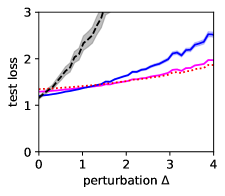
(a) Uncertain least squares loss

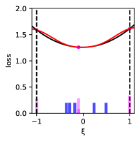
(b) Geometric interpretation

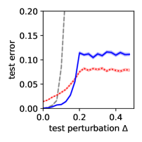
(c) MNIST classification error

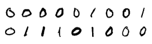
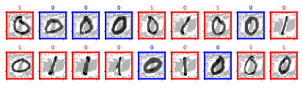
(d) (Left) unperturbed data (Center) ERM classification result (red indicates errors) (Right) SFG-DRO (Kernel DRO)

Figure 3: Uncertain least squares. (a) This plot depicts the test loss of algorithms. All error bars are in standard error. We ran $10$ independent trials. In each trial, we solved Kernel DRO to obtain $\theta$ ^∗ and tested it on a test dataset of 500 samples. We then vary the perturbation $\Delta$ from $0$ to $4$. (b) (red) is the dual optimal solution $f_{0}^{*}+f^{*}$. (black) is the function $l(\theta^{*},\cdot)$. The pink bars depict a worst-case distribution while the blue bars the empirical distribution. We can observe that $f_{0}^{*}+f^{*}$ touches loss $l(\theta^{*},\cdot)$ at the support of the worst-case distribution $P^{*}$ (pink dots). Note ${f^{*}}$ (normalized) can be viewed as a witness function of the two distributions. Classification under perturbation (c) We plot the classification error rate during test time. The $x-$axis is the perturbation magnitude allowed on the test data. For ERM, PGD, and SFG-DRO (Kernel DRO), we train $5$ independent models. Each model is tested on $500$ randomly sampled images. (d) We visualize the predictions of ERM and SFG-DRO on the perturbed images with perturbation magnitude $\Delta=0.2$. Blue frames indicate correct predictions while the red ones indicate errors.

5 NUMERICAL STUDIES

This section showcases the applicability of Kernel DRO (and hence SFG-DRO) and discusses the robustness-optimality trade-off. Our purpose is not to benchmark state-of-art performances or to demonstrate the superiority of a specific algorithm. Indeed, we believe both RO and DRO are elegant theoretical frameworks that have their specific use cases. We note that our theory can be applied to a broader scope of applications than the examples here, such as stochastic optimal control. See the appendix for more experimental results. The code is available at https://github.com/jj-zhu/kdro.

Distributionally robust solution to uncertain least squares.

We first consider a robust least squares problem adapted from El Ghaoui and Lebret (1997), which demonstrated an important application of RO to statistical learning historically. (See also (Boyd et al., 2004, Ch. 6.4).) The task is to minimize the objective $\|A\theta-b\|_{2}^{2}$ w.r.t. $\theta$. $A$ is modeled by $A(\xi)=A_{0}+\xi A_{1}$, where $\xi\in\mathcal{X}$ is uncertain, $\mathcal{X}=[-1,1]$, and $A_{0},A_{1}\in\mathbb{R}^{10\times 10},b\in\mathbb{R}^{10}$ are given. We compare Kernel DRO against using (a) empirical risk minimization (ERM; also known as sample average approximation) that minimizes $\frac{1}{N}\sum_{i=1}^{N}{\|A(\xi_{i})\ \theta-b\|_{2}^{2}}$, (b) worst-case RO via SDP from El Ghaoui and Lebret (1997). We consider a data-driven setting with given samples $\{\xi_{i}\}_{i=1}^{N}$ with the Kernel DRO formulation $\min_{\theta}\max_{P\in\mathcal{P},\mu\in\mathcal{C}}{\mathbb{E}}_{\xi\sim P}\ \|A(\xi)\ \theta-b\|_{2}^{2}\quad\operatorname*{\mathrm{subject}\ \mathrm{to}}\int\phi dP=\mu,$ where we choose the ambiguity set to be the $\epsilon$-norm-ball in the RKHS (Table 1).

Empirical samples $\{\xi_{i}\}_{i=1}^{N}(N=10)$ are generated uniformly from $[-0.5,0.5]$. We then apply Kernel DRO formulation (7). To test the solution, we create a distribution shift by generating test samples from $[-0.5\cdot(1+\Delta),0.5\cdot(1+\Delta)]$, where $\Delta$ is a perturbation varying within $[0,4]$. Figure 3a shows this comparison. As the perturbation increases, ERM quickly lost robustness. On the other hand, RO is the most robust with the trade-off of being conservative. As expected, Kernel DRO achieves some level of optimality while retaining robustness.

We then ran Kernel DRO with fewer empirical samples ($N=5$) to show the geometric interpretations. We plot the optimal dual solution $f^{*}_{0}+f^{*}$ in Figure 3b. Recall it is an over-estimator of the loss $l(\theta,\cdot)$. We solve the inner moment problem (see appendix) to obtain a worst-case distribution $P^{*}$. Comparing $P^{*}$ with $\hat{P}$, we can observe the adversarial behavior of the worst-case distribution. See the caption for more description. From Figure 3b, we can see that the intuition of Kernel DRO is to flatten the loss curve using a smooth function.

Distributionally robust learning under adversarial perturbation.

We now demonstrate the framework of SFG-DRO in Algorithm 1 in a non-convex setting. For simplicity, we consider a MNIST binary classification task with a two-layer neural network. We emphasize that the deliberate choice of this simple architecture ablates factors known to implicitly influence robustness, such as regularization and dropout. The data set contains images of zero and one (i.e., two classes). Each image $x$ is represented by $x\in[0,1]^{28\times 28}$. The test data is perturbed by an unknown disturbance, i.e., $\tilde{x}_{\mathrm{test}}:=x+\delta$ where $x\sim P_{\mathrm{test}}$ is the unperturbed test data and $\delta$ is the perturbation. In the plots, $\delta$ is generated by the PGD algorithm Madry et al. (2019) using projected gradient descent to find the worst-case perturbation within a box $\{\delta:\|\delta\|_{\infty}\leq\Delta\}\}$. We compared SFG-DRO (Kernel DRO) with ERM and PGD (cf. Madry et al. (2019), Madry ). Note the overall loss of PGD is an average loss instead of a worst-case one. Hence it is already less conservative than RO. We train a classification model $g_{\theta}\colon x\mapsto y$ using SFG-DRO in Algorithm 1, with the SA subroutine of Lan and Zhou (2020). During training, we set the ambiguity size of SFG-DRO as $\epsilon=0.5$ and domain $\mathcal{X}$ to be norm-balls around the training data $\mathcal{X}=\{\zeta=X+\delta:\|\delta\|_{\infty}\leq 0.5\}$ where $X$ is the training data.

Figure 3d (left) plots unperturbed test samples. Figure 3c shows the classification error rate as we increase the magnitude of the perturbation $\Delta$. We observe that ERM attains good performance when there is no test-time perturbation but quickly underperforms as the noise level increases. PGD is the most robust under large perturbation, but has the worst nominal performance. SFG-DRO possesses improved robustness while its performance under no perturbation does not become much worse. This is consistent with our theoretical insights into RO and DRO.

6 OTHER RELATED WORK AND DISCUSSION

This paper uses similar techniques of reformulating min-max programs as in Ben-Tal et al. (2015), Bertsimas et al. (2017), but our ambiguity set is constructed in an RKHS. Duchi et al. (2020) proposed variational approximations to marginal DRO to treat covariate shift in supervised learning. The authors of Zhu et al. (2020) used kernel mean embedding for the inner moment problem (but not DRO) and proved the statistical consistency of the solution. The work of Staib and Jegelka (2019) used insights from DRO to motivate a regularizer for kernel ridge regression. DRO has been also applied to Bayesian optimization in Rontsis et al. (2020), Kirschner et al. (2020), where the latter work used MMD ambiguity sets of distributions over discrete spaces. In terms of scalability, recent works such as Sinha et al. (2020), Li et al. (2019), Namkoong and Duchi (2016) also explored DRO for modern machine learning tasks. To the best of our knowledge, no existing work contains the results such as generalized ambiguity set constructions in Table 1, 3, generalized duality theory underpinned by Theorem 3.1, or the stochastic functional gradient algorithm SFG-DRO.

In summary, this paper proves Theorem 3.1 that generalizes the classical duality theory in the literature of mathematical problem of moments and DRO. Using the density of universal RKHSs, the dual bound in Theorem 3.1 is sharp while lifting restrictions on the loss function class. The generalized primal formulations shed light on the connection between Kernel DRO and existing robust and stochastic optimization approaches. Finally, the proposed stochastic approximation algorithm SFG-DRO enables the applications of Kernel DRO to modern learning tasks.

The compactness assumption on $\mathcal{X}$ can be further extended, as universality can be extended to non-compact domains Sriperumbudur et al. (2011). In the special case of RKHS-norm-ball ambiguity sets, choosing the size $\epsilon$ can be motivated using kernel statistical testing Gretton et al. (2012). However, when DRO is used in the setting where test distributions are perturbed as in our examples, existing statistical guarantees in the literature for unperturbed settings cannot be directly applied. This is a topic of future work.

Acknowledgements

We thank Daniel Kuhn for the helpful discussion during a workshop at IPAM, UCLA. We also thank Yassine Nemmour and Simon Buchholz for sending us their feedback on the paper draft. During part of this project, Jia-Jie Zhu was supported by the European Union’s Horizon 2020 research and innovation programme under the Marie Skłodowska-Curie grant agreement No 798321. Moritz Diehl would like to acknowledge the funding support from the DFG via Project DI 905/3-1 (on robust model predictive control)

Appendix: Kernel Distributionally Robust Optimization

Appendix A PROOFS OF THEORETICAL RESULTS

Table 2 provides an overview to help readers navigate the theoretical results in this paper.

Table 2: List of the theoretical results in this paper

Theorems	Generalized Duality Theorem 3.1
	Strong duality of the inner moment problem Proposition A.1
	Interpolation property Proposition 3.1.3
	Complementarity condition Lemma A.2
	Robust representer theorem Proposition B.1
	IPM-DRO duality Corollary 3.1.1
	Kernel DRO as stochastic optimization with expectation constraint Corollary 3.1.2
Formulations	Kernel DRO primal (P) (2), dual (D) (4)
	IPM-DRO primal (3), dual (5)
	Formulations for various RKHS ambiguity sets Table 1, 3
	Stochastic program with expectation constraint formulation of Kernel DRO (6),(9)
	Program to compute worst-case distributions (23),(24),(25)
	Kernel DRO convex program by the discretization of SIP (7)
	Kernel conditional value-at-risk (8)

In general, we refer to standard texts in optimization Boyd et al. (2004), Shapiro et al. (2014), Ben-Tal et al. (2009), convex analysis Rockafellar (1970), Barvinok (2002), and functional analysis Conway (2019) for more mathematical background.

Notation.

In the proofs, we use $\mathcal{M}$ to denote the space of signed measures on $\mathcal{X}$. The dual cone of a set of signed measures $\mathcal{K}\subseteq\mathcal{M}$ is defined as $\mathcal{K}^{*}:=\{h\colon\int h\,\mathrm{d}m\geq 0,\forall m\in\mathcal{K},h\ \ \mathrm{measurable}\}.$ Using the reproducing property, we have the identity ${\int f\ dP}=\langle{f,\mu_{P}}\rangle_{\mathcal{H}}$ for $f\in\mathcal{H}$ and $P\in\mathcal{P}$, which we will frequently use in the proofs.

A.1 Proof of the Generalized Duality Theorem 3.1

We now derive our key result for Kernel DRO — the Generalized Duality Theorem, in Theorem 3.1. Let us first consider the inner moment problem of (2)

$$\sup_{P\in\mathcal{P},\mu\in\mathcal{C}}\int l\ dP\quad\operatorname*{\mathrm{subject}\ \mathrm{to}}\ \int{\phi}{\ dP}=\mu,$$ (11)

where we suppress $\theta$ in $l(\theta,\cdot)$ as we fix it for the moment. (11) generalizes the problem of moments in the sense that the constraint can be viewed as infinite-order moment constraints. Using conic duality, we obtain the strong duality of the inner moment problem.

Proposition A.1 (Strong dual to (11)).

Under Assumption 3.1, (11) is equivalent to solving

$$\min_{f_{0}\in\mathbb{R},f\in\mathcal{H}} \ \delta^{*}_{\mathcal{C}}(f)+f_{0}$$ (12)

$$\operatorname*{\mathrm{subject}\ \mathrm{to}} \ l(\xi)\leq f_{0}+f(\xi),\ \forall\xi\in\mathcal{X}$$

where $\delta^{*}_{\mathcal{C}}$ is the support function of $\mathcal{C}$, i.e., strong duality holds.

Using Proposition A.1, we can reformulate the inner moment problem in (2) to obtain Theorem 3.1. We now prove this generalized duality result for the inner moment problem in Proposition A.1. We first derive the weak dual and then prove the strong duality.

Proof.

We first relax the constraint $P\in\mathcal{P}$ to its conic hull $P\in\mathrm{co}(\mathcal{P})$. To constrain $P$ to still be a probability measure, we impose $\int{1}{\ dP(x)}=1$, which results in the primal problem equivalent to (11)

$$(P):=\max_{P\in\mathrm{co}(\mathcal{K}),\mu\in\mathcal{C}}{\int l\ dP}\quad\operatorname*{\mathrm{subject}\ \mathrm{to}}\ {\int\phi\ dP}=\mu,\ {\int 1\ dP}=1.$$

We construct the Lagrangian relaxation by associating the constraints with the dual variables ${f\in\mathcal{H},f_{0}\in\mathbb{R}}$, as well as adding the indicator function of $\mathcal{C}$. Note both sides of the constraint $\int{\phi}{\ dP}=\mu$ are functions in $\mathcal{H}$, hence the multiplier $f$ is an RKHS function.

$$\mathcal{L}(P,\mu;\ f,f_{0})={\int l\ dP}-\delta_{\mathcal{C}}(\mu)+\langle{\mu-{\int\phi\ dP},f}\rangle_{\mathcal{H}}+f_{0}(1-{\int 1\ dP})\\ ={\int l\ dP}-\delta_{\mathcal{C}}(\mu)+\langle{\mu,f}\rangle_{\mathcal{H}}-{\int f\ dP}+f_{0}-{\int f_{0}\ dP}\\ ={\int l-f-f_{0}\ dP}+\left(\langle{\mu,f}\rangle_{\mathcal{H}}-\delta_{\mathcal{C}}(\mu)\right)+f_{0}.$$ (13)

The second equality is due to the reproducing property of RKHS. The dual function is given by

$$g(f,f_{0})=\sup_{P,\mu}{\int l-f-f_{0}\ dP}+\left(\langle{\mu,f}\rangle_{\mathcal{H}}-\delta_{\mathcal{C}}(\mu)\right)+f_{0}.$$

The first term is bounded above by $0$ iff $l-f-f_{0}\in-K^{*}$. By Lemma D.1, this conic constraint is equivalent to the constraint of (12), ${l(\xi)\leq f_{0}+f(\xi),\ \forall\xi\in\mathcal{X}}$.

Finally, expressing the second term using convex conjugate $\delta^{*}_{\mathcal{C}}(f)=\sup_{\mu}\langle{\mu,f}\rangle_{\mathcal{H}}-\delta_{\mathcal{C}}(\mu)$ concludes the derivation. ∎

Strong duality can potentially be adapted from the strong duality result of moment problem, e.g., Shapiro (2001). However, we give a self-contained proof with only elementary mathematics that sheds light on the connection between the RKHS theory and distributionally robust optimization. The proof is a generalization of the Euclidean space conic duality theorem (Ben-Tal et al. (2009) Theorem A.2.1) to infinite dimensions. Figure 4 illustrates the idea of the proof.

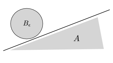
Figure 4: Illustration of the strong duality proof that uses a separating hyperplane. See the proof for detailed descriptions.

Proof.

We assume the dual optimal value of (12) is finite $(D)<\infty$. Since the converse means that the dual problem is infeasible, which implies that the primal problem is unbounded. Due to the upper semicontinuity of $l$ in Assumption 3.1, this can not happen on a compact $\mathcal{X}$.

Let us consider the Hilbert space $\mathbb{R}\times\mathcal{H}\times\mathbb{R}$ equipped with the inner product ${\langle,\rangle_{\mathbb{R}}+\langle{,}\rangle_{\mathcal{H}}+\langle,\rangle_{\mathbb{R}}}$. We construct a cone in $\mathbb{R}\times\mathcal{H}\times\mathbb{R}$

$$A=\bigg{\{}\left({\int 1\ dP},\int\phi dP,{\int l\ dP}\right):P\in\mathrm{co}(\mathcal{P})\bigg{\}},$$

where $\mathrm{co}$ again denotes conic hull.

Let $t=(P)$ denote the optimal primal value. $\forall\epsilon>0$, we construct the set

$$B_{\epsilon}=\bigg{\{}\left(1,\mu,t+\epsilon\right):\mu\in\mathcal{C}\bigg{\}},$$

which is a closed convex set with non-empty relative interior by Assumption 3.1 (i.e., Slater condition is satisfied).

It is straightforward to verify that those two sets do not intersect. Suppose $x=(x_{1},x_{2},x_{3})\in A\cap B_{\epsilon}$, this means $\exists\mu^{\prime},P^{\prime}$ such that $x_{1}=1={\int 1\ dP^{\prime}},x_{2}=\mu^{\prime}=\int\phi d{P^{\prime}}$, i.e., $\mu^{\prime},P^{\prime}$ is a primal feasible solution. Then the third coordinate of $x$ satisfies $x_{3}={\int l\ dP^{\prime}}\leq(P)<t+\epsilon=x_{3}$, which is impossible. Hence, $A\cap B_{\epsilon}=\emptyset$.

In the rest of the proof, we will show that, $\forall\epsilon>0$, the dual optimal value $(D)$ satisfies

$$(D)\leq(P)+\epsilon.$$

Combining this with weak duality $(D)\geq(P)$ will result in strong duality. We now justify this inequality.

By the separation theorem, (see, e.g., Barvinok (2002) Theorem III.3.2, 3.4), there exists a closed hyperplane that strictly separates $A$ and $B_{\epsilon}$. The separation is strict because $t+\epsilon>t={\int l\ dP}$. By the Riesz representation theorem, $\exists(f_{0},f,\tau)\in\mathbb{R}\times\mathcal{H}\times\mathbb{R},s\in\mathbb{R}$, such that

$$f_{0}+\langle{f,\mu}\rangle_{\mathcal{H}}+\tau(t+\epsilon)<s,$$

$$f_{0}{\int 1\ dP}+\langle{f,\int\phi dP}\rangle_{\mathcal{H}}+\tau{\int l\ dP}>s.$$

Plugging in $P=0$, we obtain $s<0$. Since $P$ lives in a cone, the left-hand side of the second inequality must be non-negative. Otherwise, we can scale $P$ so that the separation will fail. In summary, we have

$$f_{0}+\langle{f,\mu}\rangle_{\mathcal{H}}+\tau(t+\epsilon) <0,\forall\mu\in\mathcal{C},$$ (14)

$$f_{0}{\int 1\ dP}+\langle{f,\int\phi dP}\rangle_{\mathcal{H}}+\tau{\int l\ dP} \geq 0,\forall P\in\mathrm{co}(\mathcal{P}).$$

By Assumption 3.1 (Slater condition), the primal problem has a non-empty solution set. Because $l$ is proper and upper semi-continuous and the feasible solution set for the optimization problem is compact (see Section D) , the primal optimum is attained by the extreme value theorem. Suppose $P^{*}$ is a primal optimal solution, from the second inequality of (14),

$$f_{0}{\int 1\ dP^{*}}+\langle{f,\int\phi dP^{*}}\rangle_{\mathcal{H}}+\tau{\int l\ dP^{*}}=f_{0}+\langle{f,\mu_{P^{*}}}\rangle_{\mathcal{H}}+\tau t\geq 0.$$

Using this and the first inequality of (14), we obtain $\tau<0$. Without loss of generality, we let $\tau=-1$.

From the second inequality of (14), we have

$$f_{0}{\int 1\ dP}+\langle{f,\int\phi dP}\rangle_{\mathcal{H}}-{\int l\ dP}={\int f_{0}+f-l\ dP}\geq 0,\forall P\in\mathrm{co}(\mathcal{P}).\\$$

This tells us that $f_{0},f$ is a feasible dual solution because it satisfies the semi-infinite constraint in (12).

By the first inequality of (14),

$$f_{0}+\sup_{\mu\in\mathcal{C}}\langle{f,\mu}\rangle_{\mathcal{H}}\leq t+\epsilon,\forall\epsilon>0,$$

where the left-hand side is precisely the dual objective in (12). This implies $(D)\leq(P)+\epsilon.$ By weak duality, $(D)\geq(P)$. Therefore, strong duality holds. ∎

This proof gives us the third interpretation of the dual variables $f_{0},f$ — they define a separating hyperplane of $A$ and $B_{\epsilon}$.

Remark.

From the proof, we see that the Slater condition in Assumption 3.1 is stronger than needed be. If $\mathcal{C}$ is singleton, we can still find a convex neighborhood $W_{\epsilon}$ of the singleton $B_{\epsilon}$ since $\mathbb{R}\times\mathcal{H}\times\mathbb{R}$ is locally convex. Then $W_{\epsilon}$ and $A$ can still be strictly separated using the same technique in the proof. Hence strong duality still holds when $\mathcal{C}$ is a singleton.

Finally, we summarize the results above to prove the Kernel DRO Generalized Duality Theorem 3.1

Proof.

Theorem (3.1) is obtained by reformulating the inner moment problem in (2) using the strong duality result in Proposition A.1, i.e.,

$$\min_{\theta}\underset{P,\mu}{\sup}\bigg{\{}\int l(\theta,\xi)\ dP(\xi)\colon\int{\phi}{\ dP}=\mu,P\in\mathcal{P},\mu\in\mathcal{C}\bigg{\}}\\ =\min_{\theta}\min_{f_{0}\in\mathbb{R},f\in\mathcal{H}}\bigg{\{}f_{0}+\delta^{*}_{\mathcal{C}}(f):l(\theta,\xi)\leq f_{0}+f(\xi),\ \forall\xi\in\mathcal{X}\bigg{\}},$$ (15)

which results in formulation (4). ∎

A.2 Table 3 deriving formulations for various choices of RKHS ambiguity set $\mathcal{C}$

Table 3: Robust counterpart formulations of Kernel DRO.

RKHS ambiguity set $\mathcal{C}$	Robust counterpart formulation
norm-ball $\mathcal{C}=\{\mu\colon\|\mu-\mu_{\hat{P}}\|_{\mathcal{H}}\leq\epsilon\}$	${f_{0}+\frac{1}{N}\sum_{i=1}^{N}f(\xi_{i})+\epsilon\|{f}\|_{\mathcal{H}}}$
convex hull $\mathcal{C}=\mathrm{conv}\{\mathcal{C}_{1},\dots,\mathcal{C}_{N}\}$	${f_{0}+\max_{i}\delta^{*}_{\mathcal{C}_{i}}(f)}$
(same under closure $\mathrm{cl}\mathrm{conv}\{\mathcal{C}\}$ )
example: polytope	${f_{0}+\max_{i}f(\xi_{i})}$
$\mathcal{C}=\mathrm{conv}\{\phi(\xi_{1}),\dots,\phi(\xi_{N})\}$	(equivalent to SVMs/scenario opt. Calafiore and Campi (2006))
Minkowski sum $\sum_{i=1}^{N}C_{i}$	$f_{0}+\sum_{i=1}^{N}\delta^{*}_{\mathcal{C}_{i}}(f)$
example: $\mathcal{C}=\mathcal{C}_{1}+\mathcal{C}_{2}$	${f_{0}+\max_{i}f(\xi_{i})+\epsilon\|{f}\|_{\mathcal{H}}}$
$\mathcal{C}_{1}=\{\mu\colon\|\mu\|_{\mathcal{H}}\leq\epsilon\}$
$\mathcal{C}_{2}=\mathrm{conv}\{\phi(\xi_{1}),\dots,\phi(\xi_{N})\}$
affine combination	${f_{0}+\sum_{i=1}^{N}\alpha_{i}\delta^{*}_{\mathcal{C}_{i}}(f)}$
$\mathcal{C}=\sum_{i=1}^{N}\alpha_{i}\mathcal{C}_{i},\sum_{i=1}^{N}\alpha_{i}=1$
example: data contamination	${f_{0}+\frac{\alpha}{N}\sum_{i=1}^{N}f(\xi_{i})}+(1-\alpha)\delta^{*}_{\mathcal{C}_{Q}}(f)$
$\mathcal{C}=\{\alpha\mu_{\hat{P}}+(1-\alpha)\mu_{Q}:\mu_{Q}\in\mathcal{C}_{Q}\}$
Intersection $\mathcal{C}=\cap_{i=1}^{N}\mathcal{C}_{i}$	$f_{0}+\sum_{i=1}^{N}\delta^{*}_{\mathcal{C}_{i}}(f_{i}),\ \sum_{i=1}^{N}f_{i}=f$
multiple kernels $\mathcal{C}_{i}\subseteq\mathcal{H}_{i}$	${f_{0}+\sum_{i=1}^{N}\delta^{*}_{\mathcal{C}_{i}}(f_{i})}$ where $f_{i}\in\mathcal{H}$
example: $\mathcal{C}_{i}=\{\mu\colon\|\mu-\mu_{\hat{P}}\|_{\mathcal{H}}\leq\epsilon_{i}\}$	${f_{0}+\frac{1}{N}\sum_{i=1}^{N}\sum_{i=j}^{N}f_{i}(\xi_{j})+\epsilon\sum_{i=1}^{N}\|{f_{i}}\|_{\mathcal{H}_{i}}}$
singleton $\mathcal{C}=\left\{\sum_{i=1}^{N}{\frac{1}{N}}\phi({\xi_{i}})\right\}$	$f_{0}+\frac{1}{N}\sum_{i=1}^{N}f(\xi_{i})$ (equivalent to ERM/SAA)
entire RKHS $\mathcal{C}=\mathcal{H}$	$f_{0}+$ $\delta_{0}(f)$
	(equivalent to worst-case RO Ben-Tal et al. (2009))

We now derive the formulations of support functions for various RKHS ambiguity sets in Table 3.

(RKHS norm-ball)

Let us consider the ambiguity set of $\mathcal{C}=\{\mu\colon\|\mu-\hat{\mu}\|_{\mathcal{H}}\leq\epsilon\}$, where ${\hat{P}}=\sum_{i=1}^{N}{\frac{1}{N}}\delta_{\xi_{i}}$. The support function is given by

$$\delta^{*}_{\mathcal{C}}(f)=\sup_{\mu\in\mathcal{C}}\langle{f,\mu}\rangle_{\mathcal{H}}=\langle{f,\hat{\mu}}\rangle_{\mathcal{H}}+\sup_{\|\mu-\hat{\mu}\|_{\mathcal{H}}\leq\epsilon}\langle{f,\mu-\hat{\mu}}\rangle_{\mathcal{H}}=\langle{f,\hat{\mu}}\rangle_{\mathcal{H}}+\epsilon\|{f}\|_{\mathcal{H}}$$

where the last equality is by the Cauchy-Schwarz inequality, or alternatively by the self-duality of Hilbert norms. (Note we assume there exists some $\mu\in\mathcal{H}$ such that $\|\mu-\hat{\mu}\|_{\mathcal{H}}=\epsilon$.)

(Polytope, convex hull of ambiguity set)

The result for convex hull follows from standard support function calculus. If the ambiguity set $\mathcal{C}$ is described by the polytope $\mathrm{conv}\{\phi(\xi_{1}),\dots,\phi(\xi_{N})\}$, then $\delta^{*}_{\mathcal{C}}(f)=\max_{1\leq i\leq N}f(\xi_{i})$. Furthermore, the support function value remains the same under closure operation . The equivalence to the scenario approach in Calafiore and Campi (2006) can be seen by noticing that $\max_{1\leq i\leq N}l(\xi_{i})\leq f_{0}+\max_{1\leq i\leq N}f(\xi_{i}).$ If $\mathcal{H}$ is universal, then there exists $f_{0},f$ such that the equality is attained.

(Minkowski sum, affine combination, intersection)

Those cases follow directly from the support function calculus; cf. Ben-Tal et al. (2015).

(Kernel DRO with multiple kernels)

Let us consider multiple ambiguity sets from different RKHSs. Suppose $\mathcal{H}_{1},\dots,\mathcal{H}_{N_{h}}$ are RKHSs associated with feature maps $\phi_{1},\dots,\phi_{N_{h}}$. Let $\mathcal{C}_{1},\dots,\mathcal{C}_{N_{h}}$ be the ambiguity sets in the respective RKHSs. Kernel DRO formulation with multiple kernels is given By

$$\min_{\theta}\underset{P,\mu}{\sup}\bigg{\{}{\int l(\theta,\xi)\ dP(\xi)}\colon{\int{\phi_{i}}{\ dP}=\mu_{i},P\in\mathcal{P},\mu_{i}\in\mathcal{C}_{i}},i=1\dots N_{h}\bigg{\}},$$ (16)

Using the same proof as Proposition A.1, we have the Kernel DRO reformulation

$$\begin{aligned} &\min_{\theta,f_{0}\in\mathbb{R},f_{i}\in\mathcal{H}_{i}}&&\ f_{0}+\sum_{i=1}^{N}{\delta^{*}_{\mathcal{C}_{i}}}(f_{i})\\ &\operatorname*{\mathrm{subject}\ \mathrm{to}}&&\ l(\theta,\xi)\leq f_{0}+\sum_{i=1}^{N}f_{i}(\xi),\ \forall\xi\in\mathcal{X}\end{aligned}.$$ (17)

Hence we obtain the formulation in Table 3.

(Singleton ambiguity set $\mathcal{C}=\left\{\sum_{i=1}^{N}{\frac{1}{N}}\phi({\xi_{i}})\right\}$)

By the reproducing property, the support function of the singleton ambiguity set is given by $\delta^{*}_{\mathcal{C}}(f)=\frac{1}{N}\sum_{i=1}^{N}f(\xi_{i})$.

(If $\mathcal{C}=\mathcal{H}$, reduction to classical RO)

$\delta^{*}_{\mathcal{H}}(f)\neq\infty$ iff $f=0$. Then (4) is reduced to

$$\min_{\theta,f_{0}\in\mathbb{R}} \ f_{0}$$ (18)

$$\operatorname*{\mathrm{subject}\ \mathrm{to}} \ l(\theta,\xi)\leq f_{0},\ \forall\xi\in\mathcal{X}$$

which is the epigraphic form of the worst-case RO.

A.3 Complementarity condition and proof

Lemma A.2 (Complementarity condition).

Let $P^{*},f^{*},f^{*}_{0}$ be a set of optimal primal-dual solutions of (P) and (D), then

$${\int l-f^{*}-f_{0}^{*}\ dP^{*}}=0,\quad\delta^{*}_{\mathcal{C}}(f^{*})={\int f^{*}\ dP^{*}}$$ (19)

If $\mathcal{C}=\{\mu\colon\|\mu-\mu_{\hat{P}}\|_{\mathcal{H}}\leq\epsilon\}$, the second equality implies

$${{\int\frac{f^{*}}{\|{f^{*}}\|_{\mathcal{H}}}\ d(P^{*}-\hat{P})}=\mathrm{MMD}({P^{*},\hat{P}})},$$ (20)

which gives a second interpretation of the dual solution $f^{*}$ as a witness function.

It is well known that complementarity condition holds iff strong duality holds in the moment problem; cf. Shapiro (2001). The following is a straightforward proof.

Proof.

Plug $P^{*},f^{*},f^{*}_{0}$ into Lagrangian (13),

$${\int l\ dP^{*}}\leq{\int l-f-f_{0}\ dP^{*}}+\delta^{*}_{\mathcal{C}}(f^{*})+f_{0}^{*}\leq\delta^{*}_{\mathcal{C}}(f^{*})+f_{0}^{*}.$$

By strong duality, all inequalities above are equalities. Therefore, the first equality gives the condition $\delta^{*}_{\mathcal{C}}(f^{*})={\int f^{*}\ dP^{*}}$ while the second yields ${\int l-f^{*}-f_{0}^{*}\ dP^{*}}=0$. ∎

A.4 Proof of Proposition 3.1.3 (Interpolation property)

Proof.

Since $f_{0}^{*},f^{*}$ is a solution to the inner moment problem of Kernel DRO (12), we have $l(\theta,\xi)\leq f^{*}_{0}+f^{*}(\xi),\ \forall\xi\in\mathcal{X}$ for any given $\theta$. By the first equation in the complementarity condition (19), we have ${\int l-f^{*}-f_{0}^{*}\ dP^{*}}=0$. Hence the integrand must be zero ${P^{*}}$-a.e. ∎

A.5 Corollary 3.1.1 IPM-DRO duality

We provide a derivation using a technique alternative to the proof of Proposition A.1.

Proof.

We consider the Lagrangian

$$\mathcal{L}(P;\lambda)={\int l\ dP}-\lambda(d_{\mathcal{F}}(P,\hat{P})-\epsilon)\\ ={\int l\ dP}-\lambda\sup_{f\in\mathcal{F}}\int fd(P-\hat{P})+\lambda\epsilon\\ =\inf_{f\in\mathcal{F}}{\int l-\lambda f\ dP}+\lambda\int fd\hat{P}+\lambda\epsilon\\ \leq\inf_{f\in\mathcal{F}}\sup_{\xi\in\mathcal{X}}[{l(\xi)-\lambda f(\xi)}]+\frac{\lambda}{N}\sum_{i=1}^{N}f(\xi_{i})+\lambda\epsilon.$$ (21)

The second equality above is due to the dual representation of IPM. The last inequality is due to that the expectation is always dominated by the supremum. This results in the reformulation

$$\min_{\theta,\lambda\geq 0,f\in\mathcal{F}}\sup_{\xi\in\mathcal{X}}[{l(\xi)-\lambda f(\xi)}]+\frac{\lambda}{N}\sum_{i=1}^{N}f(\xi_{i})+\lambda\epsilon.$$

By introducing the epigraphic variable $f_{0}$, we obtain the reformulation (5). ∎

A.6 Corollary 3.1.2 Kernel DRO as stochastic optimization with expectation constraint

Using the known relationship between semi-infinite constraint and expectation constraint (see, e.g., (Tadić et al., 2006, Theorem 1)), the SI constraint in (4) is equivalent to the expectation constraint in (6).

Appendix B COMPUTATIONAL FORMULATIONS

We now provide practical plug-in formulations for computation. Specifically, we can parametrize the RKHS function $f$ by, e.g., the following methods. We note that the random feature method is well-suited for large scale problems, such as in SFG-DRO applications.

B.1 Random features

Common ways to parametrize an RKHS function include the representer theorem as well as approximations such as the random Fourier features Rahimi and Recht (2008). Recall that an RKHS function can be approximated by the finite feature expansion

$$f(\xi)\approx\hat{f}(\xi)=w^{\top}\hat{\phi}(\xi),\ \ k(x,x^{\prime})\approx\sum_{i=1}^{N}\hat{\phi}_{i}(x)\hat{\phi}_{i}(x^{\prime})$$

where $\{\hat{\phi}_{i}(x)\}_{i=1}^{N}$ are the random features, e.g., random Fourier features $\hat{\phi}_{i}(x)=\cos(w_{i}x+b_{i}),w_{i}\sim\mathrm{N}(0,\sigma^{2}),b_{i}\sim\mathrm{Uniform}[0,2\pi].$ If $x$ is a vector, then $w_{i}\sim\mathcal{N}(0,I\sigma^{2})$, and $w_{i}x$ is the dot product. See, e.g., Rahimi and Recht (2008), for more properties.

One strength of the Generalized Duality Theorem 3.1 is that it does not require the knowledge of the RKHS that the loss $l$ lives in, which is typically not available in non-kernelized models. This enables us to use approximate features for commonly used RKHSs, e.g., random Fourier feature. This is a strength of our Kernel DRO theory.

Note program (7) is a convex optimization problem with the random feature parametrization.

B.2 Distributionally robust version of representer theorem

In program (7), we may parametrize the RKHS function by $f(\cdot)=\sum_{i=1}^{N}{\beta_{i}}{k(\xi_{i},\cdot)}+\sum_{j=1}^{M}{\gamma_{j}}{k(\zeta_{j},\cdot)}$, $\|{f}\|_{\mathcal{H}}=\sqrt{\alpha^{\top}K\alpha}$, where $\alpha=(\beta_{1},\ldots,\beta_{N},\gamma_{1},\ldots,\gamma_{M})^{\top},K=[k(\eta_{i},\eta_{j})],\eta=(\xi_{1},\ldots,\xi_{N},\zeta_{1},\ldots,\zeta_{M})^{\top}$. We justify this parametrization by the following DRO version of the RKHS representer theorem Schölkopf et al. (2001).

The intuition of the following result is to restrict Kernel DRO to a smaller ambiguity set of distributions supported on $\{\zeta_{i}\}_{i=1}^{M}$ (i.e., replace $P\in\mathcal{P}$ by $P\in\mathcal{P}_{M}$, an inner approximation depending on $M$). In this setting, the ambiguity set only contains only distributions supported on (a subset of) $\zeta_{i}$. Then it suffices to parametrize $f$ in (7) by $f(\cdot)=\sum_{i=1}^{N}{\beta_{i}}{k(\xi_{i},\cdot)}+\sum_{j=1}^{M}{\gamma_{j}}{k(\zeta_{j},\cdot)}$.

Lemma B.1 (Robust representer).

Given data $\{\xi_{i}\}_{i=1}^{N}$ and the ambiguity set chosen to be a set of embeddings with the form $\sum_{j=1}^{M}\alpha_{j}\phi(\zeta_{j})$, for some $0\leq\alpha_{j}\leq 1,\sum_{j=1}^{M}\alpha_{j}=1$, and within the RKHS norm-ball $\mathcal{C}=\{\mu\colon\|\mu-\mu_{\hat{P}}\|_{\mathcal{H}}\leq\epsilon\}$. Then, it suffices to consider the RKHS function of the form $f(\cdot)=\sum_{i=1}^{N}{\beta_{i}}{k(\xi_{i},\cdot)}+\sum_{j=1}^{M}{\gamma_{j}}{k(\zeta_{j},\cdot)}$ for some $\beta_{i},\gamma_{j}\in\mathbb{R},i=1...N,j=1...M$.

Lemma B.1 states that the expansion points of the RKHS representer in (7) are exactly the support of the empirical and worst-case distributions. It extends the classical RKHS representer theorem Schölkopf et al. (2001), which uses only the empirical samples as expansion points. The implication is that, to be distributionally robust, we should choose the representers as in Lemma B.1 instead of only using empirical samples. Below is a proof that is similar to the original representer theorem.

Proof.

In (7) we consider $f=f_{s}+f_{\perp}$, where $f_{s}=\sum_{i=1}^{N}{\beta_{i}}{k(\xi_{i},\cdot)}+\sum_{j=1}^{M}{\gamma_{j}}{k(\zeta_{j},\cdot)}$ belongs to a subspace of the $\mathcal{H}$ and $f_{\perp}$ its complement. Plug in $f=f_{s}+f_{\perp}$ to (7) and note the orthogonality, we obtained

$$\min_{\theta,f_{s},f_{\perp},f_{0}} f_{0}+\frac{1}{N}\sum_{i=1}^{N}f_{s}(\xi_{i})+\epsilon(\|{f_{s}}\|_{\mathcal{H}}+\|{f_{\perp}}\|_{\mathcal{H}})$$ (22)

$$\operatorname*{\mathrm{subject}\ \mathrm{to}} \ l(\theta,\zeta_{i})\leq f_{s}(\zeta_{j})+f_{0},\ j=1\dots M.$$

It suffices to choose $f_{\perp}=0$ in this optimization problem. Hence the conclusion follows. ∎

Remark.

Note the existence of a worst case distribution in more general settings is not yet proven. The discussion here is restricted to the setting of (7).

Appendix C FURTHER NUMERICAL EXPERIMENT RESULTS

We carry out additional numerical experiments to study Kernel DRO.

C.1 Testing other variants of Kernel DRO

We empirically test the following proposed variants of Kernel DRO.

• Relaxed Kernel DRO formulation (Kernel DRO-relaxed) with constraint hold for only the empirical samples, i.e., ${l(\theta,\xi_{i})\leq f_{0}+f(\xi_{i}),\ i=1\dots N.}$

• Unconstrained Kernel DRO using Kernel CVaR in Example 4.1

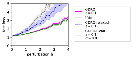
Figure 5: Comparing Kernel DRO-relaxed, Kernel DRO-KCVaR, ERM, and regular Kernel DRO. y-axis limit is adjusted to show the plot. All error bars are in standard error.

We compare Kernel DRO-relaxed with the ERM as well as the regular Kernel DRO. Compared with ERM, Kernel DRO-relaxed still possesses moderate robustness. In this case, we effectively proposed a way to apply RKHS regularization to general optimization problems, not limited to kernelized models. Hence, it may be used in practice as a finite-sample approximation to Kernel DRO.

We then test the Kernel DRO using the unconstrained objective given by Kernel CVaR. We observe no significant difference in performance between Kernel DRO-KCVaR (with small chance constraint level $\alpha$.) and regular Kernel DRO (7).

C.2 Analyzing the generalization behavior

An insight can be obtained by observing the plot of the MMD estimator between the training and test data in Figure 6 (left). As Kernel DRO with $\epsilon=0.5$ robustified against perturbation less than the level $\mathrm{MMD}=0.5$, we see this threshold was exceeded as we increase the perturbation in test data. Meanwhile, this is the same time ($\Delta\approx 1.5$) where Kernel DRO solutions start to exceed the generalization bound  ${\int l\ dP\leq f_{0}+\frac{1}{N}\sum_{i=1}^{N}f(\xi_{i})+\epsilon\|{f}\|_{\mathcal{H}}}$, see Figure 6 (right). This empirically validates our theoretical results for robustification.

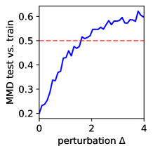
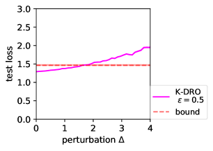
Figure 6: (Left) MMD estimator between the empirical samples and test samples. The level $\mathrm{MMD}=0.5$ is marked in red. (Right) Loss compared to the generalization bound. As the test data falls outside the robustification level $\epsilon$, the loss starts to exceed the generalization bound (red) ${f_{0}+\frac{1}{N}\sum_{i=1}^{N}f(\xi_{i})+\epsilon\|{f}\|_{\mathcal{H}}}$.

C.3 Miscellaneous details for experimental set-up

Robust least squares example.

Our experiments are implemented in Python. The convex optimization problems are solved using ECOS or MOSEK interfaced with CVXPY. In the experiments, we chose the bandwidth for the Gaussian kernel using the medium heuristic Gretton et al. (2012). $\epsilon$ in this paper are fixed to constants below $2$ for Gaussian kernels. Choosing $\epsilon$ can be further motivated by kernel statistical tests Gretton et al. (2012) and is left for future work.

Sampled $\zeta_{j}$

In applying Kernel DRO using  (7), we may obtain $\zeta_{j}$ by simply sampling in $\mathcal{X}$. $\{\zeta_{j}\}_{i}$ need not be real data, e.g., in stochastic control, they can be a grid of system states; in learning, they can be synthetic samples such as convex combinations of data $\zeta_{j}=\sum_{i=1}^{N}a_{ij}\xi_{i},a_{\cdot j}\in S_{N}$ (simplex), or perturbations $\zeta_{j}=\hat{\xi}_{i}+\Delta_{i}$ where $\Delta_{i}$ can be a small perturbation, or they can be obtained by domain knowledge of the specific application. In the setting of supervised machine learning, there is a difference between this paper’s approach of sampling $\zeta_{j}$ and commonly used data-augmentation techniques: $\zeta_{j}$ need not have the correct labels or targets. Directly training on them may have unforeseen consequences. For example, in the robust least squares experiment, we sampled the support $\zeta_{i}$ uniformly random from $[-1,1]$.

Robust learning under adversarial perturbation example.

For the MNIST robust classification example, we used a neural network with two hidden layers with $64$ units each. For the training of ERM and PGD, we used the ADAM optimization routine implemented in the PyTorch library. In Step 3 of SFG-DRO, we used random Fourier features Rahimi and Recht (2008) with $500$ features. In Step 5 of SFG-DRO, we used the SA routine from CSA algorithm Lan and Zhou (2020). While other SA routines can be used, we prefer the simplicity of CSA in that it does not use a dual variable. We set the threshold and step-size of the CSA algorithm Lan and Zhou (2020) to decay at the rate of $\frac{1}{\sqrt{k}}$ as suggested in that paper. We did not attempt further adaptive tuning of the step-sizes or the proposing distribution for $\zeta$ (we generate $3000$ samples uniformly in Step 2 of SFG-DRO), which may further improve the performance. Parameter (weights of the neural nets) averaging is used for training all models. In the visualization of the predictions in Figure 3d, we perturbed the images by the PGD method Madry et al. (2019), Madry based on the ERM loss and linear model. SFG-DRO does not have the knowledge of the perturbation method.

C.4 Computing worst-case distributions

We have proposed Kernel DRO for making the decision $\theta$ via reformulation (4). In practice, it is often useful to find the worst-case distribution $P^{*}$ (e.g., to study adversarial examples). We now propose two practical methods to compute $P^{*}$ for a given $\theta$, based on support sampling and perturbation, respectively. We illustrate the ideas in Figure 7.

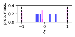
(a) Support sampling

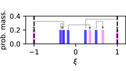
(b) Perturbation

Figure 7: Computing the worst-case distribution $P^{*}$ using (a): (23) samples possible support $\zeta_{j}$ then optimizes w.r.t. weights $\alpha$. (b): (24) moves the empirical samples directly.

Support sampling.

We consider the moment problem (11) where the distribution is restricted to discrete distributions supported on some sampled support $\{\zeta_{j}\}_{j=1}^{M}\subseteq\mathcal{X}$. For any given $\theta$,

$$\max_{\alpha\in S_{M}}\sum_{j=1}^{M}\alpha_{i}l(\theta,\zeta_{j})\quad\operatorname*{\mathrm{subject}\ \mathrm{to}}\ \bigg{\|}{\sum_{j=1}^{M}\alpha_{i}\phi(\zeta_{j})-\frac{1}{N}\sum_{i=1}^{N}\phi(\xi_{i})}\bigg{\|}_{\mathcal{H}}\leq\epsilon.\\$$ (23)

(23) can be written as a quadratically constrained program with linear objective, which admits a (strong) semidefinite program dual via what is historically known as the S-lemma Pólik and Terlaky (2007) (cf. appendix). Alternatively, (23) can be directly handled by convex solvers for a given $\theta$. Note this approach was previously used in solving the problem of moments in Zhu et al. (2020).

Perturbation.

Alternatively, we search for worst-case distributions that are perturbations of the empirical distribution. Let $d_{i}\in\mathcal{X}$ be some perturbation vector, given $\theta$,

$$\max_{\begin{subarray}{c}d_{i},i=1\dots N,\\ {\xi}_{i}+d_{i}\in\mathcal{X}\end{subarray}} \frac{1}{N}\sum_{i=1}^{N}l(\theta,{\xi}_{i}+d_{i}) \operatorname*{\mathrm{subject}\ \mathrm{to}} \bigg{\|}{\frac{1}{N}\sum_{i=1}^{N}\left(\phi({\xi}_{i}+d_{i})-\phi({\xi}_{i})\right)}\bigg{\|}_{\mathcal{H}}\leq\epsilon.$$ (24)

Compared with (23), (24) directly searches for the support of the worst-case distribution. It can be interpreted as transporting the probability mass from empirical samples $\xi_{i}$ to form the worst-case distribution. Depending on the kernel used, (24) may become a nonlinear program. However, its feasibility is guaranteed since it can always be initialized with a feasible solution $d_{i}=0$.

We now empirically examine the support sampling method (23) and perturbation method (24) to recover the worst-case distribution. Since both programs (23) and (24) search for the worst-case distribution within a subset of all distributions, their optimal values lower-bound the true worst-case risk (P) in (11), i.e., with finite samples, they are optimistic bound.

Under the experimental setting as in Figure 3b, we ran Kernel DRO with fewer empirical samples ($N=5$). After we obtain the Kernel DRO solution $\theta^{*}$, we plug it into (23) and (24), respectively, to compute the worst-case distribution $P^{*}$. Figure 7 plots the results. Note (23) is a convex optimization problem, while (24) results in a nonlinear program (with Gaussian kernel). Nonetheless, we solve it with an always-feasible initialization $d_{i}=0$.

C.5 SDP dual via S-lemma

We consider a discretized version of the primal moment problem in (23) where the distribution is constrained to be a discrete distribution. We rewrite (23) as a quadratically constrained program using the plug-in estimator of MMD,

$$\max_{\alpha} \sum_{i=1}^{M}\alpha_{i}l(\zeta_{i})$$

$$\operatorname*{\mathrm{subject}\ \mathrm{to}} \alpha^{\top}K_{z}\alpha-2\frac{1}{N}\alpha^{\top}K_{zx}\mathbf{1}+\frac{1}{N^{2}}\mathbf{1}^{\top}K_{x}\mathbf{1}\leq\epsilon^{2}$$

$$\sum_{i=1}^{M}\alpha_{i}=1,\alpha_{i}\geq 0,i=1\dots M.$$

This is a quadratically constrained linear objective convex optimization problem, where the Gram matrix $K_{z}$ almost always has exponentially decaying eigenvalues. By applying S-lemma Pólik and Terlaky (2007), this program can be reformulated as the following SDP,

$$\min_{\lambda\geq 0,x,y\geq 0,t} t$$ (25)

$$\operatorname*{\mathrm{subject}\ \mathrm{to}} \begin{bmatrix}\lambda P&-\lambda q-\frac{1}{2}(l+x\cdot\mathbbm{1}+y)\\ (-\lambda q-\frac{1}{2}(l+x\cdot\mathbbm{1}+y))^{\top}&t-\lambda\epsilon^{2}+x+\lambda r\end{bmatrix}\geq 0,$$

where $P:=K_{z},\ q:=\frac{1}{N}\mathbf{1}^{\top}K_{zx},\ r:=\frac{1}{N^{2}}\mathbf{1}^{\top}K_{x}\mathbf{1},$ and $K_{z}=[k(\zeta_{i},\zeta_{j})]_{ij},K_{zx}=[k(\zeta_{i},\hat{\xi}_{j})]_{ij},K_{x}=[k(\hat{\xi}_{i},\hat{\xi}_{j})]_{ij},l=[l(\zeta_{1}),\dots,l(\zeta_{M})]^{\top}$.

Appendix D SUPPORTING LEMMAS

We establish a few technical results that are used in the proofs.

D.1 Reducing conic constraint to infinite constraint

To derive the semi-infinite constraint in (12), we need a standard result from the literature of the moment problem. We give a self-contained proof below.

Lemma D.1.

Let $K^{*}$ be the dual cone to the probability simplex $\mathcal{P}$. The conic constraint ${l-f-f_{0}\in-K^{*}}$ is equivalent to

$$l(\theta,\xi)\leq f_{0}+f(\xi),\ \forall\xi\in\mathcal{X}.$$ (26)

Proof.

“$\implies$”: Let us consider the set of all Dirac measures on $\mathcal{X}$, $\mathcal{D}:=\{\delta_{\xi}\colon\xi\in\mathcal{X}\}$. For any $\xi\in\mathcal{X}$, we have

$$l(\xi)-f_{0}-f(\xi)=\int l-f_{0}-fd\delta_{\xi}\leq 0.$$

Hence sufficiency.

“$\impliedby$”: Suppose there exists $P^{\prime}\in\mathrm{co}(\mathcal{P})$ such that $\int l-f_{0}-fdP^{\prime}>0$. Without loss of generality, we assume $P^{\prime}\in\mathcal{P}$, or we can normalize it to be a probability measure. Then,

$$0<\int l-f_{0}-fdP^{\prime}\leq\sup_{\xi\in\mathcal{X}}l(\xi)-f_{0}-f(\xi)\leq 0.$$

The second inequality is due to that expectation is always less than or equal to the supremum. The last inequality holds because $l$ is u.s.c. This double inequality is impossible, hence $l-f_{0}-f\in-K^{*}$. ∎

Note an extension of this result to generating classes other than all Dirac measures $\mathcal{D}$ can be proved using Choquet theory, cf. (Shapiro et al., 2014, Proposition 6.66) (Popescu, 2005, Lemma 3.1), as well as in Shapiro (2001), Rogosinski .

D.2 Compactness of the ambiguity set

We now prove the compactness of the ambiguity set. We use the mean map notation $\mathcal{T}:P\mapsto\mu_{P}$ to denote a map between the space of $\mathcal{P}$ equipped with MMD, and $\mathcal{H}$ equipped with its norm. Let us denote the image of a subset $\mathcal{K}$ of measures under $\mathcal{T}$ by $\mathcal{T}(\mathcal{K}):=\{\mu_{P}\mid P\in\mathcal{K}\}\subseteq\mathcal{H}$. If $\mathcal{H}$ is universal, then MMD is a metric. By the definition of MMD, $\mathcal{T}$ is an isometry (i.e., distance-preserving map) between $\mathcal{P}$ and $\mathcal{H}$.

Lemma D.2.

$\mathcal{T}(\mathcal{P})$ is compact if $\mathcal{X}$ is compact.

Proof.

If $\mathcal{X}$ is compact, by Prokhorov’s theorem $\mathcal{P}$ is compact. Since $\mathcal{T}$ is an isometry, $\mathcal{T}(\mathcal{P})$ is compact. ∎

It is straightforward to verify that $\mathcal{T}(\mathcal{P})$ is convex.

Lemma D.3.

Let $C_{P}=\mathcal{C}\cap\mathcal{T}(\mathcal{P})$. If $\mathcal{X}$ is compact, under Assumption 3.1, $C_{p}$ is compact.

Proof.

By the Krein-Milman theorem, the convexity and compactness of $\mathcal{T}(\mathcal{P})$ (proved in the previous lemma) imply that $\mathcal{T}(\mathcal{P})$ is closed. By Assumption 3.1, $\mathcal{C}$ is closed, which results in the closedness of $C_{p}$. Since $C_{p}$ is a closed subset of a compact set $\mathcal{T}(\mathcal{P})$, it is compact. ∎

Recall that we denote the feasible set of probability measures, i.e., ambiguity set, for primal Kernel DRO (2) by $\mathcal{K}_{\mathcal{C}}={\{P\colon\int\phi\ dP=\mu,\mu\in\mathcal{C},P\in\mathcal{P}\}}$. It is convex by straightforward verification. Let us derive the following compactness property of the ambiguity set.

Lemma D.4.

If $\mathcal{X}$ is compact, under Assumption 3.1, $\mathcal{K}_{\mathcal{C}}$ is compact.

Proof.

We first note $\mathcal{K}_{\mathcal{C}}=\mathcal{T}^{-1}(C_{p})$ and $\mathcal{T}$ is an isometric isomorphism (i.e., bijective isometry) between $\mathcal{K}_{\mathcal{C}}$ and $C_{p}$. Then $\mathcal{K}_{\mathcal{C}}$ is compact since $C_{p}$ is compact. ∎

References

- Baes et al. (2011) Michel Baes, Michael Bürgisser, and Arkadi Nemirovski. A randomized Mirror-Prox method for solving structured large-scale matrix saddle-point problems. arXiv:1112.1274 [math], December 2011.
- Barvinok (2002) Alexander Barvinok. A Course in Convexity, volume 54. American Mathematical Soc., 2002.
- Ben-Tal et al. (2009) Aharon Ben-Tal, Laurent El Ghaoui, and Arkadi Nemirovski. Robust Optimization, volume 28. Princeton University Press, 2009.
- Ben-Tal et al. (2013) Aharon Ben-Tal, Dick den Hertog, Anja De Waegenaere, Bertrand Melenberg, and Gijs Rennen. Robust Solutions of Optimization Problems Affected by Uncertain Probabilities. Management Science, 59(2):341–357, February 2013. ISSN 0025-1909, 1526-5501. doi: 10.1287/mnsc.1120.1641.
- Ben-Tal et al. (2015) Aharon Ben-Tal, Dick den Hertog, and Jean-Philippe Vial. Deriving robust counterparts of nonlinear uncertain inequalities. Mathematical Programming, 149(1):265–299, February 2015. ISSN 1436-4646. doi: 10.1007/s10107-014-0750-8.
- Bertsimas and Popescu (2005) Dimitris Bertsimas and Ioana Popescu. Optimal Inequalities in Probability Theory: A Convex Optimization Approach. SIAM Journal on Optimization, 15(3):780–804, January 2005. ISSN 1052-6234, 1095-7189. doi: 10.1137/S1052623401399903.
- Bertsimas et al. (2017) Dimitris Bertsimas, Nathan Kallus, and Vishal Gupta. Data-Driven Robust Optimization. Springer Berlin Heidelberg, 2017. ISBN 1010701711258. doi: 10.1007/s10107-017-1125-8.
- Bietti et al. (2019) Alberto Bietti, Grégoire Mialon, Dexiong Chen, and Julien Mairal. A Kernel Perspective for Regularizing Deep Neural Networks. arXiv:1810.00363 [cs, stat], May 2019.
- Blanchet et al. (2019) Jose Blanchet, Yang Kang, and Karthyek Murthy. Robust Wasserstein Profile Inference and Applications to Machine Learning. Journal of Applied Probability, 56(03):830–857, September 2019. ISSN 0021-9002, 1475-6072. doi: 10.1017/jpr.2019.49.
- Boser et al. (1992) Bernhard E. Boser, Isabelle M. Guyon, and Vladimir N. Vapnik. A training algorithm for optimal margin classifiers. In Proceedings of the Fifth Annual Workshop on Computational Learning Theory, pages 144–152, 1992.
- Boyd et al. (2004) Stephen Boyd, Stephen P. Boyd, and Lieven Vandenberghe. Convex Optimization. Cambridge University Press, March 2004. ISBN 978-0-521-83378-3.
- Calafiore and Campi (2006) G.C. Calafiore and M.C. Campi. The scenario approach to robust control design. IEEE Transactions on Automatic Control, 51(5):742–753, May 2006. ISSN 2334-3303. doi: 10.1109/TAC.2006.875041.
- Carratino et al. (2018) Luigi Carratino, Alessandro Rudi, and Lorenzo Rosasco. Learning with SGD and Random Features. In S. Bengio, H. Wallach, H. Larochelle, K. Grauman, N. Cesa-Bianchi, and R. Garnett, editors, Advances in Neural Information Processing Systems 31, pages 10192–10203. Curran Associates, Inc., 2018.
- Christmann and Steinwart (2007) Andreas Christmann and Ingo Steinwart. Consistency and robustness of kernel-based regression in convex risk minimization. Bernoulli, 13(3):799–819, August 2007. ISSN 1350-7265. doi: 10.3150/07-BEJ5102.
- Conway (2019) John B Conway. A course in functional analysis, volume 96. Springer, 2019.
- Cortes and Vapnik (1995) Corinna Cortes and Vladimir Vapnik. Support-vector networks. Machine learning, 20(3):273–297, 1995.
- Dai et al. (2014) Bo Dai, Bo Xie, Niao He, Yingyu Liang, Anant Raj, Maria-Florina F Balcan, and Le Song. Scalable Kernel Methods via Doubly Stochastic Gradients. In Z. Ghahramani, M. Welling, C. Cortes, N. D. Lawrence, and K. Q. Weinberger, editors, Advances in Neural Information Processing Systems 27, pages 3041–3049. Curran Associates, Inc., 2014.
- Delage and Ye (2010) Erick Delage and Yinyu Ye. Distributionally Robust Optimization Under Moment Uncertainty with Application to Data-Driven Problems. Operations Research, 58(3):595–612, June 2010. ISSN 0030-364X, 1526-5463. doi: 10.1287/opre.1090.0741.
- Duchi et al. (2016) John Duchi, Peter Glynn, and Hongseok Namkoong. Statistics of robust optimization: A generalized empirical likelihood approach. arXiv preprint arXiv:1610.03425, 2016.
- Duchi et al. (2020) John Duchi, Tatsunori Hashimoto, and Hongseok Namkoong. Distributionally Robust Losses for Latent Covariate Mixtures. arXiv:2007.13982 [cs, stat], July 2020.
- El Ghaoui and Lebret (1997) Laurent El Ghaoui and Hervé Lebret. Robust Solutions to Least-Squares Problems with Uncertain Data. SIAM Journal on Matrix Analysis and Applications, 18(4):1035–1064, October 1997. ISSN 0895-4798. doi: 10.1137/S0895479896298130.
- Gao and Kleywegt (2016) Rui Gao and Anton J. Kleywegt. Distributionally Robust Stochastic Optimization with Wasserstein Distance. arXiv:1604.02199 [math], July 2016.
- Gretton et al. (2012) Arthur Gretton, Karsten M. Borgwardt, Malte J. Rasch, Bernhard Schölkopf, and Alexander Smola. A kernel two-sample test. Journal of Machine Learning Research, 13(Mar):723–773, 2012.
- Guerra Vázquez et al. (2008) F. Guerra Vázquez, J. J. Rückmann, O. Stein, and G. Still. Generalized semi-infinite programming: A tutorial. Journal of Computational and Applied Mathematics, 217(2):394–419, August 2008. ISSN 0377-0427. doi: 10.1016/j.cam.2007.02.012.
- Isii (1962) Keiiti Isii. On sharpness of tchebycheff-type inequalities. Annals of the Institute of Statistical Mathematics, 14(1):185–197, December 1962. ISSN 1572-9052. doi: 10.1007/BF02868641.
- Iyengar (2005) Garud N. Iyengar. Robust Dynamic Programming. Mathematics of Operations Research, 30(2):257–280, 2005. ISSN 0364-765X.
- Kirschner et al. (2020) Johannes Kirschner, Ilija Bogunovic, Stefanie Jegelka, and Andreas Krause. Distributionally Robust Bayesian Optimization. arXiv:2002.09038 [cs, stat], March 2020.
- Lan and Zhou (2020) Guanghui Lan and Zhiqiang Zhou. Algorithms for stochastic optimization with function or expectation constraints. Computational Optimization and Applications, February 2020. ISSN 0926-6003, 1573-2894. doi: 10.1007/s10589-020-00179-x.
- Lasserre (2002) Jean B. Lasserre. Bounds on measures satisfying moment conditions. The Annals of Applied Probability, 12(3):1114–1137, 2002.
- Li et al. (2019) Jiajin Li, Sen Huang, and Anthony Man-Cho So. A First-Order Algorithmic Framework for Wasserstein Distributionally Robust Logistic Regression. arXiv:1910.12778 [cs, math, stat], October 2019.
- Madry et al. (2019) Aleksander Madry, Aleksandar Makelov, Ludwig Schmidt, Dimitris Tsipras, and Adrian Vladu. Towards Deep Learning Models Resistant to Adversarial Attacks. arXiv:1706.06083 [cs, stat], September 2019.
- (32) Zico Kolter and Aleksander Madry. Adversarial Robustness - Theory and Practice. http://adversarial-ml-tutorial.org/.
- Mohajerin Esfahani and Kuhn (2018) Peyman Mohajerin Esfahani and Daniel Kuhn. Data-driven distributionally robust optimization using the Wasserstein metric: Performance guarantees and tractable reformulations. Mathematical Programming, 171(1):115–166, September 2018. ISSN 1436-4646. doi: 10.1007/s10107-017-1172-1.
- Namkoong and Duchi (2016) Hongseok Namkoong and John C Duchi. Stochastic Gradient Methods for Distributionally Robust Optimization with f-divergences. In D. D. Lee, M. Sugiyama, U. V. Luxburg, I. Guyon, and R. Garnett, editors, Advances in Neural Information Processing Systems 29, pages 2208–2216. Curran Associates, Inc., 2016.
- Nilim and El Ghaoui (2005) Arnab Nilim and Laurent El Ghaoui. Robust Control of Markov Decision Processes with Uncertain Transition Matrices. Operations Research, 53(5):780–798, October 2005. ISSN 0030-364X, 1526-5463. doi: 10.1287/opre.1050.0216.
- Pólik and Terlaky (2007) Imre Pólik and Tamás Terlaky. A Survey of the S-Lemma. SIAM Review, 49(3):371–418, January 2007. ISSN 0036-1445, 1095-7200. doi: 10.1137/S003614450444614X.
- Popescu (2005) Ioana Popescu. A Semidefinite Programming Approach to Optimal-Moment Bounds for Convex Classes of Distributions. Mathematics of Operations Research, 30(3):632–657, August 2005. ISSN 0364-765X, 1526-5471. doi: 10.1287/moor.1040.0137.
- Rahimi and Recht (2008) Ali Rahimi and Benjamin Recht. Random Features for Large-Scale Kernel Machines. In J. C. Platt, D. Koller, Y. Singer, and S. T. Roweis, editors, Advances in Neural Information Processing Systems 20, pages 1177–1184. Curran Associates, Inc., 2008.
- Rockafellar (1970) R. Tyrrell Rockafellar. Convex Analysis. Number 28. Princeton university press, 1970.
- Rockafellar and Uryasev (2000) R. Tyrrell Rockafellar and Stanislav Uryasev. Optimization of conditional value-at-risk. Journal of risk, 2:21–42, 2000.
- (41) W W Rogosinski. Moments of Non-Negative Mass. page 28.
- Rontsis et al. (2020) Nikitas Rontsis, Michael A. Osborne, and Paul J. Goulart. Distributionally Ambiguous Optimization for Batch Bayesian Optimization. Journal of Machine Learning Research, 21(149):1–26, 2020. ISSN 1533-7928.
- Scarf (1958) Herbert Scarf. A min-max solution of an inventory problem. Studies in the mathematical theory of inventory and production, 1958.
- Schölkopf et al. (2001) B. Schölkopf, R. Herbrich, and A. J. Smola. A generalized representer theorem. In D. Helmbold and R. Williamson, editors, Annual Conference on Computational Learning Theory, number 2111 in Lecture Notes in Computer Science, pages 416–426, Berlin, 2001. Springer.
- Schölkopf et al. (2000) Bernhard Schölkopf, Alex J. Smola, Robert C. Williamson, and Peter L. Bartlett. New support vector algorithms. Neural computation, 12(5):1207–1245, 2000.
- Shapiro (2001) Alexander Shapiro. On Duality Theory of Conic Linear Problems. In Panos Pardalos, Miguel Á. Goberna, and Marco A. López, editors, Semi-Infinite Programming, volume 57, pages 135–165. Springer US, Boston, MA, 2001. ISBN 978-1-4419-5204-2 978-1-4757-3403-4. doi: 10.1007/978-1-4757-3403-4_7.
- Shapiro et al. (2014) Alexander Shapiro, Darinka Dentcheva, and Andrzej Ruszczyński. Lectures on Stochastic Programming: Modeling and Theory. SIAM, 2014.
- Sinha et al. (2020) Aman Sinha, Hongseok Namkoong, Riccardo Volpi, and John Duchi. Certifying Some Distributional Robustness with Principled Adversarial Training. arXiv:1710.10571 [cs, stat], May 2020.
- Smola et al. (2007) Alex Smola, Arthur Gretton, Le Song, and Bernhard Schölkopf. A hilbert space embedding for distributions. In International Conference on Algorithmic Learning Theory, pages 13–31. Springer, 2007.
- Sriperumbudur et al. (2011) Bharath K. Sriperumbudur, Kenji Fukumizu, and Gert R. G. Lanckriet. Universality, Characteristic Kernels and RKHS Embedding of Measures. Journal of Machine Learning Research, 12(Jul):2389–2410, 2011. ISSN ISSN 1533-7928.
- Sriperumbudur et al. (2012) Bharath K. Sriperumbudur, Kenji Fukumizu, Arthur Gretton, Bernhard Schölkopf, and Gert R. G. Lanckriet. On the empirical estimation of integral probability metrics. Electronic Journal of Statistics, 6:1550–1599, 2012. ISSN 1935-7524. doi: 10.1214/12-EJS722.
- Staib and Jegelka (2019) Matthew Staib and Stefanie Jegelka. Distributionally robust optimization and generalization in kernel methods. In Advances in Neural Information Processing Systems, pages 9131–9141, 2019.
- Steinwart and Christmann (2008) Ingo Steinwart and Andreas Christmann. Support Vector Machines. Springer Science & Business Media, 2008.
- Tadić et al. (2006) Vladislav B. Tadić, Sean P. Meyn, and Roberto Tempo. Randomized Algorithms for Semi-Infinite Programming Problems. In Giuseppe Calafiore and Fabrizio Dabbene, editors, Probabilistic and Randomized Methods for Design under Uncertainty, pages 243–261. Springer, London, 2006. ISBN 978-1-84628-095-5. doi: 10.1007/1-84628-095-8_9.
- Van Parys et al. (2016) Bart P. G. Van Parys, Paul J. Goulart, and Daniel Kuhn. Generalized Gauss inequalities via semidefinite programming. Mathematical Programming, 156(1-2):271–302, March 2016. ISSN 0025-5610, 1436-4646. doi: 10.1007/s10107-015-0878-1.
- Vandenberghe et al. (2007) Lieven. Vandenberghe, Stephen. Boyd, and Katherine. Comanor. Generalized Chebyshev Bounds via Semidefinite Programming. SIAM Review, 49(1):52–64, January 2007. ISSN 0036-1445. doi: 10.1137/S0036144504440543.
- Virmaux and Scaman (2018) Aladin Virmaux and Kevin Scaman. Lipschitz regularity of deep neural networks: Analysis and efficient estimation. In S. Bengio, H. Wallach, H. Larochelle, K. Grauman, N. Cesa-Bianchi, and R. Garnett, editors, Advances in Neural Information Processing Systems 31, pages 3835–3844. Curran Associates, Inc., 2018.
- Wang et al. (2016) Zizhuo Wang, Peter W. Glynn, and Yinyu Ye. Likelihood robust optimization for data-driven problems. Computational Management Science, 13(2):241–261, April 2016. ISSN 1619-697X, 1619-6988. doi: 10.1007/s10287-015-0240-3.
- Wei et al. (2020) Bo Wei, William B. Haskell, and Sixiang Zhao. The CoMirror algorithm with random constraint sampling for convex semi-infinite programming. Annals of Operations Research, September 2020. ISSN 1572-9338. doi: 10.1007/s10479-020-03766-7.
- Wong and Kolter (2018) Eric Wong and Zico Kolter. Provable defenses against adversarial examples via the convex outer adversarial polytope. In International Conference on Machine Learning, pages 5286–5295. PMLR, 2018.
- Xu et al. (2009) Huan Xu, Constantine Caramanis, and Shie Mannor. Robustness and regularization of support vector machines. Journal of machine learning research, 10(7), 2009.
- Xu (2020) Yangyang Xu. Primal-Dual Stochastic Gradient Method for Convex Programs with Many Functional Constraints. SIAM Journal on Optimization, 30(2):1664–1692, January 2020. ISSN 1052-6234, 1095-7189. doi: 10.1137/18M1229869.
- Zhao and Guan (2018) Chaoyue Zhao and Yongpei Guan. Data-driven risk-averse stochastic optimization with Wasserstein metric. Operations Research Letters, 46(2):262–267, March 2018. ISSN 01676377. doi: 10.1016/j.orl.2018.01.011.
- Zhu et al. (2020) Jia-Jie Zhu, Wittawat Jitkrittum, Moritz Diehl, and Bernhard Schölkopf. Worst-Case Risk Quantification under Distributional Ambiguity using Kernel Mean Embedding in Moment Problem. arXiv:2004.00166 [cs, eess, math], March 2020.
- Zymler et al. (2013) Steve Zymler, Daniel Kuhn, and Berç Rustem. Distributionally robust joint chance constraints with second-order moment information. Mathematical Programming, 137(1-2):167–198, February 2013. ISSN 0025-5610, 1436-4646. doi: 10.1007/s10107-011-0494-7.