Non-Negative Bregman Divergence Minimization
for Deep Direct Density Ratio Estimation

Abstract

Density ratio estimation (DRE) is at the core of various machine learning tasks such as anomaly detection and domain adaptation. In existing studies on DRE, methods based on Bregman divergence (BD) minimization have been extensively studied. However, BD minimization when applied with highly flexible models, such as deep neural networks, tends to suffer from what we call train-loss hacking, which is a source of overfitting caused by a typical characteristic of empirical BD estimators. In this paper, to mitigate train-loss hacking, we propose a non-negative correction for empirical BD estimators. Theoretically, we confirm the soundness of the proposed method through a generalization error bound. Through our experiments, the proposed methods show a favorable performance in inlier-based outlier detection.

1 Introduction

Density ratio estimation (DRE) has attracted a great deal of attention as an essential task in various machine learning problems, such as regression under a covariate shift (Shimodaira, 2000; Reddi et al., 2015), learning with noisy labels (Liu & Tao, 2014; Fang et al., 2020), anomaly detection (Smola et al., 2009; Hido et al., 2011; Abe & Sugiyama, 2019), two-sample testing (Keziou & Leoni-Aubin, 2005; Kanamori et al., 2010; Sugiyama et al., 2011a), causal inference (Uehara et al., 2020), change point detection (Kawahara & Sugiyama, 2009), and binary classification only from positive and unlabeled data (PU learning; Kato et al., 2019). For instance, anomaly detection is not easy to apply based on standard machine learning methods since anomalous data are often scarce; however, we can solve this by estimating the density ratio when anomaly-free unlabeled test data are available (Hido et al., 2008).

Among the various approaches to DRE, we focus on the Bregman divergence (BD) minimization framework (Bregman, 1967; Sugiyama et al., 2011b), which is a general framework that unifies various DRE methods, such as moment matching (Huang et al., 2007; Gretton et al., 2009), probabilistic classification (Qin, 1998; Cheng & Chu, 2004), density matching (Nguyen et al., 2010), and density-ratio fitting (Kanamori et al., 2009). Kato et al. (2019) proposed using the risk of PU learning for DRE, which also falls within this framework (Appendix A).

Existing methods have mainly adopted linear-in-parameter models for DRE (Kanamori et al., 2012). On the other hand, recent studies in machine learning have suggested that deep neural networks achieve significantly high performances for various tasks, such as computer vision (CV) (Krizhevsky et al., 2012) and natural language processing (NLP) (Bengio et al., 2001). These findings motivate us to use deep neural networks for DRE.

However, when using deep neural networks in combination with empirical BD minimization, we often observe a serious overfitting problem as experimentally demonstrated in Figure 2 of Section 5.1 and Figure 4 of Appendix F.1.1. We observe that this is mainly because a model of the density ratio $r(X)=\frac{q(X)}{p(X)}$ between two probability densities $p$ and $q$ becomes large for high-dimensional data when using a flexible model. As the intuition behind this phenomenon, a flexible model can overfit the samples generated from $p(X)$ as if there were no common support between $p(X)$ and $q(X)$ (Figure 1). This hypothesis is inspired by Kiryo et al. (2017), which reports a similar problem in PU learning. In the case of DRE through BD minimization, we conjecture that this phenomenon is caused by the objective function that monotonically decreases with respect to $r(X)$, misleading the model $r(X)$ to take on as large a value as possible on the specific data points $X$. Note that even if $r(X)$ is bounded, this phenomenon still manifests as the model takes on the largest possible value within its output range. Rhodes et al. (2020) and Ansari et al. (2020) independently found related problems in DRE. Whereas Kiryo et al. (2017) and Rhodes et al. (2020) call their phenomena overfitting and density-chasm problem, respectively, we refer to our problem as train-loss hacking because this problem is specific to methods based on BD minimization, and we can still observe this issue even when the true $r(x)=\frac{p(x)}{q(x)}$ is not significantly large. This problem is discussed in more detail in Section 2.3 (Figure 1).

Owing to this property, training a density ratio model with a flexible model tends to result in either a diverging empirical BD estimator or a model sticking to the upper bound of its output range. For instance, when the empirical BD divergence is not lower bounded, it often numerically diverges to negative infinity. Even when the loss function has a lower bound (see BKL and Bounded uLSIF introduced in Sections 2.2 and 5.1), the trained models tend to stick to the largest possible value of their output ranges (Bounded uLSIF in Figure 2 and BKL-NN in Figure 4). Although train-loss hacking has rarely been discussed in existing studies on DRE, this problem is often encountered while using deep neural networks, as experimentally shown in Section 5.1. One reason for this is that the existing studies use linear-in-parameter models (Kanamori et al., 2012) or simple shallow neural networks (Nam & Sugiyama, 2015; Abe & Sugiyama, 2019) for the density ratio models, which tend to be inflexible in that they do not cause such a phenomenon.

To mitigate the train-loss hacking, we propose a general procedure to modify the empirical BD estimator. First, from the empirical BD divergence, we separate the term causing the train-loss hacking. We then apply a non-negative correction to the term to make the model consistent with a constraint that should be satisfied within the population. Our idea of this correction is inspired by Kiryo et al. (2017). However, their idea of a non-negative correction is only applicable to the binary classification setting; thus, we require a non-trivial rewriting of the BD to generalize the approach to our problem. We call our proposed objective function the non-negative BD (nnBD). The proposed method can be regarded as a generalization of the method proposed by Kiryo et al. (2017).

Our main contributions are (1) proposal of a general procedure to modify an empirical BD estimator to enable DRE with flexible models, (2) theoretical justification of the proposed estimator, and (3) experimental validation of the proposed method using benchmark data.

2 Problem setting

Let $\mathcal{X}^{\mathrm{nu}}\subseteq\mathbb{R}^{d}$ and $\mathcal{X}^{\mathrm{de}}\subseteq\mathbb{R}^{d}$ be the spaces of the $d$-dimensional covariates. Here, “nu” and “de” indicate the numerator and denominator. Let $p_{\mathrm{nu}}$ and $p_{\mathrm{de}}$ be the probability densities over $\mathcal{X}^{\mathrm{nu}}$ and $\mathcal{X}^{\mathrm{de}}$, respectively. We have independent and identically distributed (i.i.d.) samples from these distributions: ${\bf{X}}^{\mathrm{nu}}=\big{\{}X^{\mathrm{nu}}_{j}\big{\}}^{n_{\mathrm{nu}}}_{j=1}\overset{\mathrm{i.i.d.}}{\sim}p_{\mathrm{nu}}$ and ${\bf{X}}^{\mathrm{de}}=\big{\{}X^{\mathrm{de}}_{i}\big{\}}^{n_{\mathrm{de}}}_{i=1}\overset{\mathrm{i.i.d.}}{\sim}p_{\mathrm{de}}$.

Basic assumption and goal.

Throughout this paper, we assume that $p_{\mathrm{nu}}(X)$ and $p_{\mathrm{de}}(X)$ are strictly positive over $\mathcal{X}^{\mathrm{nu}}$ and $\mathcal{X}^{\mathrm{de}}$, respectively. We also assume $\mathcal{X}^{\mathrm{nu}}\subseteq\mathcal{X}^{\mathrm{de}}$, which is a typical assumption in the literature on DRE, e.g., Section 2.1 of Kanamori et al. (2009). The goal of DRE is to estimate $r^{*}(x)=\frac{p_{\mathrm{nu}}(x)}{p_{\mathrm{de}}(x)}$ from the samples $\bf{X}^{\mathrm{nu}}$ and $\bf{X}^{\mathrm{de}}$.

Additional notation.

Let $\mathbb{E}_{\mathrm{nu}}$ and $\mathbb{E}_{\mathrm{de}}$ denote the expectations with respect to $p_{\mathrm{nu}}(X)$ and $p_{\mathrm{de}}(X)$, respectively; in addition, $\hat{\mathbb{E}}_{\mathrm{nu}}$ and $\hat{\mathbb{E}}_{\mathrm{de}}$ denote the sample averages over $\big{\{}X^{\mathrm{nu}}_{j}\big{\}}^{n_{\mathrm{nu}}}_{j=1}$ and $\big{\{}X^{\mathrm{de}}_{i}\big{\}}^{n_{\mathrm{de}}}_{i=1}$, respectively.

Table 1: Summary of DRE methods (Sugiyama et al., 2011b). For PULogLoss, we use $C<\frac{1}{\overline{R}}$.

Method	$f(t)$	Lower bound of $\widehat{\mathrm{BD}}_{f}$	Reference
LSIF	$(t-1)^{2}/2$	Not bounded	Kanamori et al. (2009)
Kernel Mean Matching	$(t-1)^{2}/2$	Not bounded	Gretton et al. (2009)
UKL	$t\log(t)-t$	Not bounded	Nguyen et al. (2010)
KLIEP	$t\log(t)-t$	Not bounded	Sugiyama et al. (2008)
BKL (LR)	$t\log(t)-(1+t)\log(1+t)$	Bounded	Hastie et al. (2001)
PULogLoss	$C\log\left(1-t\right)+Ct\left(\log\left(t\right)-\log\left(1-t\right)\right)$ for $0<t<1$	Not bounded	Kato et al. (2019)

2.1 Density ratio matching by BD minimization

Among existing DRE methods, we focus on density ratio matching through BD minimization (DRM-BD; Sugiyama et al., 2011b), which is a framework that unifies various DRE methods (Gretton et al., 2009; Sugiyama et al., 2008; Kanamori et al., 2009; Nguyen et al., 2010).

DRM-BD estimates the density ratio by minimizing the objective function derived as follows: Let $(b_{r},B_{r})\subset[0,\infty)$, and let $f:(b_{r},B_{r})\to\mathbb{R}$ be a twice continuously differentiable convex function with a bounded derivative $\partial f$ (Table 1). We quantify the discrepancy from the true density ratio function $r^{*}$ to a density ratio model $r$ by

$$\mathrm{BD}_{f}(r^{*}\|r):=\mathbb{E}_{\mathrm{de}}\left[\partial f(r(X))r(X)-f(r(X))\right]\\ \qquad-\mathbb{E}_{\mathrm{nu}}\left[\partial f(r(X))\right]$$ (1)

which is equal to the BD (Bregman, 1967) defined as $\mathbb{E}_{\mathrm{de}}[\ddot{\mathrm{BD}}_{f}(r^{*}(X)\|r(X))]$, where

$$\ddot{\mathrm{BD}}_{f}(t^{*}\|t):=f(t^{*})-f(t)-\partial f(t)(t^{*}-t),$$

ignoring the constant $\overline{\mathrm{BD}}=\mathbb{E}_{\mathrm{de}}\big{[}f(r^{*}(X))\big{]}$. Then, given a hypothesis class $\mathcal{H}$, DRM-BD estimates $r^{*}$ using a minimizer of the sample analog of (1):

$$\widehat{\mathrm{BD}}_{f}(r):=\hat{\mathbb{E}}_{\mathrm{de}}\Big{[}\partial f\big{(}r(X_{i})\big{)}r(X_{i})-f\big{(}r(X_{i})\big{)}\Big{]}\\ \qquad-\hat{\mathbb{E}}_{\mathrm{nu}}\Big{[}\partial f\big{(}r(X_{j})\big{)}\Big{]}.$$ (2)

2.2 Examples of DRE

Sugiyama et al. (2011b) showed that BD minimization can unify various DRE methods. Furthermore, Menon & Ong (2016) showed an equivalence between conditional probability estimation and DRE from the BD minimization perspective. In addition, by generalizing the results of du Plessis et al. (2015) and Kato et al. (2019), we derive a novel method for DRE from PU learning in Appendix B. We summarize the DRE methods in Table 1. Here, the empirical risks of least-square importance fitting (LSIF), unnormalized Kullback–Leibler (UKL) divergence, binary Kullback–Leibler (BKL) divergence, and PU learning with log Loss (PULogLoss) are given as

$$\widehat{\mathrm{BD}}_{\mathrm{LSIF}}(r):=\frac{1}{2}\hat{\mathbb{E}}_{\mathrm{de}}[r^{2}(X_{i})]-\hat{\mathbb{E}}_{\mathrm{nu}}[r(X_{j})],$$

$$\widehat{\mathrm{BD}}_{\mathrm{UKL}}(r):=\hat{\mathbb{E}}_{\mathrm{de}}\left[r(X_{i})\right]-\hat{\mathbb{E}}_{\mathrm{nu}}\left[\log\big{(}r(X_{j})\big{)}\right],$$

$$\widehat{\mathrm{BD}}_{\mathrm{BKL}}(r):=-\hat{\mathbb{E}}_{\mathrm{de}}\left[\mathrm{BKL1}(X_{i})\right]-\hat{\mathbb{E}}_{\mathrm{nu}}\left[\mathrm{BKL2}(X_{j})\right],$$

$$\widehat{\mathrm{BD}}_{\mathrm{PU}}(r):=-\hat{\mathbb{E}}_{\mathrm{de}}\left[\log\big{(}1-r(X_{i})\big{)}\right]$$

$$\ \ \ \ \ \ \ \ \ \ \ \ \ \ \ +C\hat{\mathbb{E}}_{\mathrm{nu}}\left[-\log\big{(}r(X_{j})\big{)}+\log\big{(}1-r(X_{j})\big{)}\right],$$

where $0<C<\frac{1}{\overline{R}}$, $\overline{R}$ is an upper bound on $r^{*}$, $\mathrm{BKL1}(x)=\log\left(\frac{1}{1+r(x)}\right)$, and $\mathrm{BKL2}(x)=\log\left(\frac{r(x)}{1+r(x)}\right)$. Here, $\widehat{\mathrm{BD}}_{\mathrm{LSIF}}(r)$ and $\widehat{\mathrm{BD}}_{\mathrm{PU}}(r)$ correspond to LSIF and PULogLoss, respectively. We can derive the Kullback–Leibler importance estimation procedure (KLIEP) and logistic regression-based DRE (LR) from $\widehat{\mathrm{BD}}_{\mathrm{UKL}}(r)$ and $\widehat{\mathrm{BD}}_{\mathrm{BKL}}(r)$. In $\widehat{\mathrm{BD}}_{\mathrm{PU}}(r)$, we restrict the model’s output to be within $(0,1)$ and the estimated model $r$ becomes an estimator of $Cr^{*}$. Details of these methods are provided in Appendix A.

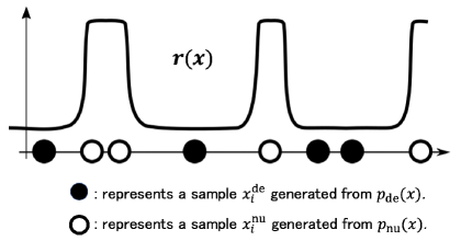
Figure 1: Illustration of the train-loss hacking phenomenon. Given finite data points, a sufficiently flexible model $r$ can easily make the second term of the objective function $\widehat{\mathrm{BD}}_{f}$ largely negative, resulting in an unreasonable minimizer.

2.3 Train-loss hacking problem

DRM-BD with neural networks often suffers from an overfitting. For instance, in Section 5.1, we show that the LSIF with neural networks suffers from a serious overfitting issue. We conjecture that a conceivable cause of the overfitting in DRE-BD is the train-loss hacking. This hypothesis is inspired by Kiryo et al. (2017), which tackled a similar problem in PU learning; see Appendix C for a brief review.

Train-loss hacking is a phenomenon in which $r(X_{j})$ increases to a large value for $\big{\{}X^{\mathrm{nu}}_{j}\big{\}}^{n_{\mathrm{nu}}}_{j=1}\overset{\mathrm{i.i.d.}}{\sim}p_{\mathrm{nu}}(x)$ when a model is trained to minimize an objective function consisting of multiple separate samples. Recall that, in the case of DRE-BD, the objective function (2) consists of two empirical averages. Among these two, we can make the second term $-\hat{\mathbb{E}}_{\mathrm{nu}}\big{[}\partial f\big{(}r(X_{j})\big{)}\big{]}$ small by making the model to take as large values as possible at the specific input points $\bf{X}^{\mathrm{nu}}$ (Figure 1). In fact, since $f$ is a convex function, $\partial f$ is an increasing function; hence, this term monotonically decreases as $r$ increases in $\bf{X}^{\mathrm{nu}}$. As a result, when there is no lower bound on $-\hat{\mathbb{E}}_{\mathrm{nu}}\big{[}\partial f\big{(}r(X_{j})\big{)}\big{]}$, it often numerically diverges to negative infinity. Even when there is a lower bound on $-\hat{\mathbb{E}}_{\mathrm{nu}}\big{[}\partial f\big{(}r(X_{j})\big{)}\big{]}$, $r(X_{j})$ tends to take on the largest possible value of its output range at the points $\bf{X}^{\mathrm{nu}}$. Naively “capping” the model’s output, e.g., composing $r(X)$ with $\max\{\cdot,B\}$ where $B>0$ is a constant, fails to remedy the issue as the model still tends to stick to its largest possible value. We experimentally demonstrate this by implementing the Bounded uLSIF (Figure 2).

This is a critical issue, since merely making the output large on $\bf{X}^{\mathrm{nu}}$ is unlikely to be a reasonable training criterion for DRE, and it may only lead to an unreasonable density ratio estimator (Figure 1). The issue becomes salient when the model has a high flexibility. If the hypothesis class has an extremely limited flexibility, this may not be an issue since the remaining term $\hat{\mathbb{E}}_{\mathrm{de}}\Big{[}\partial f\big{(}r(X_{i})\big{)}r(X_{i})-f\big{(}r(X_{i})\big{)}\Big{]}$ is likely to introduce a trade-off. However, when highly flexible models such as deep neural networks are employed, the model can easily fit to $\bf{X}^{\mathrm{nu}}$ and $\bf{X}^{\mathrm{de}}$ separately (Figure 1).

3 Deep direct DRE based on non-negative risk estimator

Although DRE with flexible models suffers from serious train-loss hacking, we still have a strong motivation to use them for applications, such as CV and NLP. In this section, we describe our approach to modify the DRM-BD objective function to mitigate the train-loss hacking problem.

3.1 Non-negative BD

To alleviate the train-loss hacking problem, we propose a non-negative BD estimator that modifies an empirical BD estimator (2) to be robust against the problem. The proposed method is inspired by Kiryo et al. (2017), which suggested a non-negative correction to the empirical risk of PU learning based on the knowledge that a part of the population risk is non-negative. However, in DRE, it is not straightforward to employ this approach because we do not know which part of the population risk (1) is non-negative. In this paper, by assuming an upper bound $\overline{R}$ on the density ratio $r^{*}$, we detect which part of the risk of DRE (1) is non-negative in the population. Then, we apply a non-negative correction to an empirical BD estimator (2) based on the non-negativity of the corresponding part of the population risk. This non-negative correction also corresponds to a generalization of non-negative PU learning (Kiryo et al., 2017).

To enable our approach to mitigate the train-loss hacking, we apply the following assumption:

Assumption 1.

The density ratio $r^{*}$ is bounded from above, i.e., $\overline{R}=\sup_{X\in\mathcal{X}^{\mathrm{de}}}r^{*}(X)<\infty$.

Then, we arbitrarily specify a constant $C$ such that $0<C<\frac{1}{\overline{R}}$. Using $C$, we make the following assumption.

Assumption 2.

A function $\tilde{f}$ defined by

$$\partial f(t)=C\big{(}\partial f(t)t-f(t)\big{)}+\tilde{f}(t)$$ (3)

is bounded from above.

Then, we rewrite the DRM-BD objective (1) as

$$\mathrm{BD}_{f}(r^{*}\|r)=\underbrace{\mathbb{E}_{\mathrm{de}}[\ell_{1}(r(X))]-C\mathbb{E}_{\mathrm{nu}}[\ell_{1}(r(X))]}_{\text{($\ast$)}}\\ \qquad\qquad\qquad+\mathbb{E}_{\mathrm{nu}}\ell_{2}(r(X))-(1-C)A,$$ (4)

where $\ell_{1}$ and $\ell_{2}$ are

$$\ell_{1}(t) :=\partial f(t)t-f(t)+A,\quad\ell_{2}(t):=-\tilde{f}(t),$$

and $A$ is a constant such that $\ell_{1}(t)\geq 0$ for all $t\in(b_{r},B_{r})$. Now, we make the following observation.

Observation.

The ($\ast$) part in (4) is non-negative since both $\ell_{1}$ and $p_{\mathrm{de}}-Cp_{\mathrm{nu}}$ are non-negative under Assumption 1 and $0<C<\frac{1}{\overline{R}}$.

Based on this observation, we propose using the following modified empirical risk:

$$\widehat{\mathrm{nnBD}}_{f}(r):=\left(\hat{\mathbb{E}}_{\mathrm{de}}\big{[}\ell_{1}(r(X_{i}))\big{]}-C\hat{\mathbb{E}}_{\mathrm{nu}}\big{[}\ell_{1}(r(X_{j}))\big{]}\right)_{+}\\ \quad+\hat{\mathbb{E}}_{\mathrm{nu}}\big{[}\ell_{2}(r(X_{j}))\big{]}$$ (5)

where $(\cdot)_{+}:=\max\{0,\cdot\}$. Note that the nonnegativity of ($\ast$) is always satisfied in the population quantity; however, it can be violated in finite samples, allowing for train-loss hacking. Our deep direct DRE (D3RE) is based on minimizing $\widehat{\mathrm{nnBD}}_{f}(r)$ over a hypothesis class of the density ratio $\mathcal{H}\subset\{r:\mathbb{R}^{d}\to(b_{r},B_{r})\}$, where $0\leq b_{r}<\overline{R}<B_{r}$.

Instantiations of the D3RE objective functions.

The above strategy can be instantiated with various functions $f$ proposed for DRM-BD. Here, we introduce nnBD corresponding to LSIF, UKL, BKL, and PULogLoss as follows:

$$\widehat{\mathrm{nnBD}}_{\mathrm{LSIF}}(r):=-\hat{\mathbb{E}}_{\mathrm{nu}}\left[r(X_{j})-\frac{C}{2}r^{2}(X_{j})\right]$$

$$\ \ \ \ \ \ \ \ \ \ \ \ \ \ \ \ \ \ \ \ \ \ +\left(\frac{1}{2}\hat{\mathbb{E}}_{\mathrm{de}}\left[r^{2}(X_{i})\right]-\frac{C}{2}\hat{\mathbb{E}}_{\mathrm{nu}}\left[r^{2}(X_{j})\right]\right)_{+},\ \quad$$

$$\widehat{\mathrm{nnBD}}_{\mathrm{UKL}}(r):=-\hat{\mathbb{E}}_{\mathrm{nu}}\left[\log\big{(}r(X_{j})\big{)}-Cr(X_{j})\right]$$

$$\ \ \ \ \ \ \ \ \ \ \ \ \ \ \ \ \ \ \ \ \ \ \ \ \ \ \ \ \ \ \ \ \ +\left(\hat{\mathbb{E}}_{\mathrm{de}}\left[r(X_{i})\right]-C\hat{\mathbb{E}}_{\mathrm{nu}}\left[r(X_{j})\right]\right)_{+},$$

$$\widehat{\mathrm{nnBD}}_{\mathrm{BKL}}(r):=-\hat{\mathbb{E}}_{\mathrm{nu}}\left[\mathrm{BKL2}(X_{j})+C\mathrm{BKL1}(X_{j})\right]$$

$$\ \ \ \ \ \ \ \ \ +\Bigg{(}-\hat{\mathbb{E}}_{\mathrm{de}}\left[\mathrm{BKL1}(X_{i})\right]+C\hat{\mathbb{E}}_{\mathrm{nu}}\left[\mathrm{BKL1}(X_{j})\right]\Bigg{)}_{+},$$

$$\widehat{\mathrm{nnBD}}_{\mathrm{PU}}(r):=-C\hat{\mathbb{E}}_{\mathrm{nu}}\left[\log\big{(}r(X_{j})\big{)}\right]$$

$$+\left(C\hat{\mathbb{E}}_{\mathrm{nu}}\left[\log\big{(}1-r(X_{j})\big{)}\right]-\hat{\mathbb{E}}_{\mathrm{de}}\left[\log\big{(}1-r(X_{i})\right]\right)_{+}.$$

More detailed derivation of $\tilde{f}$ is in Appendix B.

The algorithm for D3RE is described in Algorithm 1. For training with a large amount of data, we adopt a stochastic optimization by splitting the dataset into mini-batches. In stochastic optimization, we separate the samples into $N$ mini-batches as $(\big{\{}X^{\mathrm{nu}}_{i}\big{\}}^{n_{\mathrm{nu},j}}_{i=1},\big{\{}X^{\mathrm{de}}_{i}\big{\}}^{n_{\mathrm{de},j}}_{i=1})$ ($j=1,\ldots,N$, where $n_{\mathrm{nu},j}$ and $n_{\mathrm{de},j}$ are the sample sizes for each mini-batch. Then, we consider the sample average in each mini-batch. Let $\hat{\mathbb{E}}^{j}_{\mathrm{nu}}$ and $\hat{\mathbb{E}}^{j}_{\mathrm{de}}$ be sample averages over $\big{\{}X^{\mathrm{nu}}_{i}\big{\}}^{n_{\mathrm{nu},j}}_{i=1}$ and $\big{\{}X^{\mathrm{de}}_{i}\big{\}}^{n_{\mathrm{de},j}}_{i=1}$. In addition, we use regularization, such as L1 and L2 penalties, as denoted by $\mathcal{R}(r)$.

To improve the performance, we can heuristically employ gradient ascent from Kiryo et al. (2017) when $\hat{\mathbb{E}}_{\mathrm{de}}\big{[}\ell_{1}(r(X))\big{]}-C\hat{\mathbb{E}}_{\mathrm{nu}}\big{[}\ell_{1}(r(X))\big{]}$ becomes less than $0$, i.e., the model is updated in the direction that increases the term. Note that gradient ascent is not essential in D3RE, and we can obtain similar results even without it (see experiments in Appendix F.1.2). We recommend practitioners to use a gradient ascent and those concerned with a theoretical guarantee to use a plain gradient descent.

Choice of $C$.

Although we use an upper bound of the density ratio in the formulation, we do not require a tight one. The main role of the upper bound is to prevent the density ratio model from diverging, and as long as we successfully prevent divergence, the proposed algorithms work well. We find that D3RE is robust against a loose specification of the upper bound to a certain extent in our experiment (the right graph in Figure 2 of Section 5.1). Thus, in practice, selecting $C$ does not require accurate knowledge of $\overline{R}$. In fact, in inlier-based outlier detection experiments, the proposed methods under a loose specification of the upper bound achieve a preferable performance. However, selecting a hyper-parameter $C$ that is much smaller than $1/\overline{R}$ may damage the empirical performance as shown in Section 5.1. This, of course, does not mean that $1/\overline{R}$ should not be small; if $1/\overline{R}$ is small, $C$ can also be small.

Non-negative PU learning.

Kiryo et al. (2017) proposed a non-negative correction for PU learning (nnPU). In this paper, we propose a non-negative correction for DRE, inspired by Kiryo et al. (2017); however, our extension is nontrivial because the relationship between DRE and PU learning has not been well understood. Another contribution of this paper is that it clarifies the relationship between DRE and PU learning, as described in Appendix A and Section 5. We find that the class-prior in PU learning corresponds to the upper bound of $r^{*}$ in DRE, and that as Sugiyama et al. (2012) generalized DRE in terms of BD divergence minimization, the risk of PU learning can also be generalized through BD divergence minimization. This finding had been implied by Kato et al. (2019), although it had not been formally shown. This finding clarifies the relationship between DRE and PU learning, and thus makes it possible to apply the non-negative correction to DRE, such as nnPU.

Algorithm 1 D3RE

  Input: Training data $\big{\{}X^{\mathrm{nu}}_{j}\big{\}}^{n_{\mathrm{nu}}}_{j=1}$ and $\big{\{}X^{\mathrm{de}}_{i}\big{\}}^{n_{\mathrm{de}}}_{i=1}$, the algorithm for stochastic optimization such as Adam (Kingma & Ba, 2015), the learning rate $\gamma$, the regularization coefficient $\lambda$ and function $\mathcal{R}(r)$, and a constant $C>0$.

  Output: A density ratio estimator $\hat{r}$.

  while No stopping criterion has been met: do

     Create $N$ mini-batches

$$\left\{\left(\big{\{}X^{\mathrm{nu}}_{j}\big{\}}^{n_{\mathrm{nu},k}}_{j=1},\big{\{}X^{\mathrm{de}}_{i}\big{\}}^{n_{\mathrm{de},k}}_{i=1}\right)\right\}^{N}_{k=1}.$$

     for $k=1$ to $N$ do

        if $\hat{\mathbb{E}}^{k}_{\mathrm{de}}\big{[}\ell_{1}(r(X))\big{]}-C\hat{\mathbb{E}}^{k}_{\mathrm{nu}}\big{[}\ell_{1}(r(X))\big{]}\geq 0$: then

           Gradient decent: set gradient

$$\nabla_{r}\big{\{}\hat{\mathbb{E}}^{k}_{\mathrm{nu}}\big{[}\ell_{2}(r(X))\big{]}+\hat{\mathbb{E}}^{k}_{\mathrm{de}}\big{[}\ell_{1}(r(X))\big{]}$$

$$\ \ \ \ \ \ \ \ \ \ \ \ \ \ \ \ \ \ \ \ -C\hat{\mathbb{E}}^{k}_{\mathrm{nu}}\big{[}\ell_{1}(r(X))\big{]}+\lambda\mathcal{R}(r)\big{\}}.$$

        else

           Gradient ascent: set gradient

$$\nabla_{r}\big{\{}-\hat{\mathbb{E}}^{k}_{\mathrm{de}}\big{[}\ell_{1}(r(X))\big{]}+C\hat{\mathbb{E}}^{k}_{\mathrm{nu}}\big{[}\ell_{1}(r(X))\big{]}+\lambda\mathcal{R}(r)\big{\}}.$$

        end if

        Update $r$ with the gradient and the learning rate $\gamma$.

     end for

  end while

3.2 Motivation and intuitive justification of D3RE

Here, we describe how the above non-negative risk correction alleviates the train-loss hacking problem.

D3RE and an unbounded empirical risk.

First, we consider the case where the empirical BD is unbounded. First, we assume the following on $\tilde{f}(t)$ of (3). Assumption 2 is satisfied by most of the loss functions which appear in the previously proposed DRE methods (see Appendix B for examples). Under Assumption 2, because $\tilde{f}(t)$ is bounded above, the train-loss hacking $-\hat{\mathbb{E}}_{\mathrm{nu}}\Big{[}\partial f\big{(}r(X_{j})\big{)}\Big{]}\to-\infty$ to minimize the empirical risk (2) is caused by

$$-\hat{\mathbb{E}}_{\mathrm{nu}}\Big{[}C\left\{\partial f(r(X_{j}))r(X_{j})-f(r(X_{j}))\right\}\Big{]}\to-\infty$$

because

$$\underbrace{-\hat{\mathbb{E}}_{\mathrm{nu}}\Big{[}\partial f\big{(}r(X_{j})\big{)}\Big{]}}_{\text{$\rightarrow-\infty$}}=\underbrace{-\hat{\mathbb{E}}_{\mathrm{nu}}\Big{[}\tilde{f}(r(X_{j}))\Big{]}}_{\text{Bounded}}\\ \underbrace{-\hat{\mathbb{E}}_{\mathrm{nu}}\Big{[}C\left\{\partial f(r(X_{j}))r(X_{j})-f(r(X_{j}))\right\}\Big{]}}_{\text{$\rightarrow-\infty$}}.$$

This observation implies that our non-negative correction (5) prevents train-loss hacking by effectively introducing the correction to the problematic term ($\ast$ in (4)).

D3RE and a bounded empirical risk.

Next, we consider the case where $\partial f\big{(}r(X_{j})$ or model $r(x)$ is bounded. Even in these cases, train-loss hacking can occur. For instance, if $\partial f(t)=\log(t)-\log(1+t)$ (BKL), $\partial f(t)$ is upper-bounded by $0$, and $-\hat{\mathbb{E}}_{\mathrm{nu}}\big{[}\partial f\big{(}r(X_{j})\big{)}\big{]}$ does not diverge to $-\infty$. However, we can infinitely decrease $-\hat{\mathbb{E}}_{\mathrm{nu}}\big{[}\partial f\big{(}r(X_{j})\big{)}\big{]}$ to $0$ by making $r(X_{j})\to\infty$, which causes train-loss hacking. On the other hand, when $r(x)$ is upper-bounded, we can minimize $-\hat{\mathbb{E}}_{\mathrm{nu}}\big{[}\partial f\big{(}r(X_{j})\big{)}\big{]}$ by training $r(X_{j})$ to stick to the upper bound at $\big{\{}X^{\mathrm{nu}}_{i}\big{\}}^{n_{\mathrm{nu}}}_{i=1}$. Therefore, the upper-bounding $\partial f\big{(}r(X_{j})$ or model $r(x)$ does not solve the train-loss hacking. However, for these cases, the proposed non-negative risk correction approach is empirically shown to be effective, as shown in Figure 2 of Section 5.1 and Figure 4 of Appendix F.1.1. In these results, Bounded LSIF and BKL correspond to the upper bounding of the model $r(x)$ and $\partial f\big{(}r(X_{j})$, respectively. Experimentally, DRE methods without the non-negative correction fail to learn the density ratio, while the non-negative correction succeeded in stabilizing the performance.

4 Theoretical justification of D3RE

In this section, we confirm the validity of D3RE by providing a generalization error bound. We derive two types of guarantees, one in terms of the BD risk and the other the $L^{2}$-distance. Given $n\in\mathbb{N}$ and a distribution $p$, we define the Rademacher complexity $\mathcal{R}_{n}^{p}$ of a function class $\mathcal{H}$ as $\mathcal{R}_{n}^{p}(\mathcal{H}):=\mathbb{E}_{p}\mathbb{E}_{\sigma}\left[\sup_{r\in\mathcal{H}}\left|\frac{1}{n}\sum_{i=1}^{n}\sigma_{i}r(X_{i})\right|\right]$, where $\{\sigma_{i}\}_{i=1}^{n}$ are independent uniform sign variables and $\{X_{i}\}_{i=1}^{n}\overset{\mathrm{i.i.d.}}{\sim}p$. We omit $r^{*}$ from the notation $\mathrm{BD}_{f}$ when there is no ambiguity.

4.1 Generalization error bound on BD

Let $I_{r}:=(b_{r},B_{r})$. Theorem 4 in Appendix H provides a generalization error bound in terms of the Rademacher complexities of a hypothesis class and the following assumption.

Assumption 3.

Following (i)–(iv) hold:

(i)

there exists an empirical risk minimizer $\hat{r}\in\operatorname*{arg\,min}_{r\in\mathcal{H}}\widehat{\mathrm{nnBD}}_{f}(r)$ and a population risk minimizer $\bar{r}\in\operatorname*{arg\,min}_{r\in\mathcal{H}}\mathrm{BD}_{f}(r)$;

(ii)

${B_{\ell}}:=\sup_{t\in I_{r}}\{\max\{|\ell_{1}(t)|,|\ell_{2}(t)|\}\}<\infty$;

(iii)

$\ell_{1}$ (resp. $\ell_{2}$) is $L_{\ell_{1}}$-Lipschitz (resp. $L_{\ell_{2}}$-Lipschitz) on $I_{r}$;

(iv)

$\inf_{r\in\mathcal{H}}(\mathbb{E}_{\mathrm{de}}-C\mathbb{E}_{\mathrm{nu}})\ell_{1}(r(X))>0$.

For the boundedness and Lipschitz continuity in Assumption 3 to hold for the loss functions involving a logarithm (UKL, BKL, PU), a technical assumption $b_{r}>0$ is sufficient.

Then, we introduce Assumption 4 (Golowich et al., 2019, Theorem 1) to bound the complexity of the hypothesis class.

Assumption 4 (Neural networks with bounded complexity).

The probability densities $p_{\mathrm{nu}}$ and $p_{\mathrm{de}}$ have bounded supports: $\sup_{x\in\mathcal{X}^{\mathrm{de}}}\|x\|<\infty$, and a hypothesis class $\mathcal{H}$ consists of real-valued neural networks of depth $L$ over the domain $\mathcal{X}$, where each parameter matrix $W_{j}$ has the Frobenius norm at most $B_{W_{j}}\geq 0$ and $1$-Lipschitz activation functions $\varphi_{j}$ that are positive-homogeneous (i.e., $\varphi_{j}$ is applied element-wise and $\varphi_{j}(\alpha t)=\alpha\varphi_{j}(t)$ for all $\alpha\geq 0$).

Under Assumption 4, Lemma 3 in Appendix I reveals $\mathcal{R}_{n_{\mathrm{nu}}}^{p_{\mathrm{nu}}}(\mathcal{H})=\mathcal{O}(1/\sqrt{n_{\mathrm{nu}}})$ and $\mathcal{R}_{n_{\mathrm{de}}}^{p_{\mathrm{de}}}(\mathcal{H})=\mathcal{O}(1/\sqrt{n_{\mathrm{de}}})$. By combining these results with Theorem 4 in Appendix H, we obtain the following theorem.

Theorem 1 (Generalization error bound for D3RE).

Under Assumptions 3 and 4, for any $\delta\in(0,1)$, we have with probability at least $1-\delta$,

$$\mathrm{BD}_{f}(\hat{r})-\mathrm{BD}_{f}(\bar{r})\leq\frac{\kappa_{1}}{\sqrt{n_{\mathrm{de}}}}+\frac{\kappa_{2}}{\sqrt{n_{\mathrm{nu}}}}$$

$$\ \ \ +2(1+C){B_{\ell}}\exp\left(-\frac{2\alpha^{2}}{({B_{\ell}}^{2}/n_{\mathrm{de}})+(C^{2}{B_{\ell}}^{2}/n_{\mathrm{nu}})}\right)$$

$$\ \ \ +{B_{\ell}}\sqrt{8\left(\frac{1}{n_{\mathrm{de}}}+\frac{(1+C)^{2}}{n_{\mathrm{nu}}}\right)\log\frac{1}{\delta}},$$

where $\kappa_{1},\kappa_{2}$ are constants that depend on $C,f,B_{p_{\mathrm{de}}},B_{p_{\mathrm{nu}}},L$, and $B_{W_{j}}$.

See Remark 5 in Appendix H for more explicit forms of $\kappa_{1}$ and $\kappa_{2}$. This generalization error bound provides theoretical guarantees for various applications. For instance, by defining $f(t)=\log\left(1-t\right)+Ct\left(\log\left(t\right)-\log\left(1-t\right)\right)$ for $0<t<1$, $\mathrm{BD}_{f}(r)$ becomes the risk functional of PU learning (see Appendix A for the derivation). Then, the generalization error bound provides a classification error bound for PU learning, which is a special case of the binary classification problem Kiryo et al. (2017). Note that the dependency of the bound on $f,B_{p_{\mathrm{de}}},B_{p_{\mathrm{nu}}},L$, and $B_{W_{j}}$ is typical for classification with Lipschitz functions (Bartlett & Mendelson, 2003, Corollary 15). The third term of the RHS corresponds to the bias caused by the use of non-negative correction.

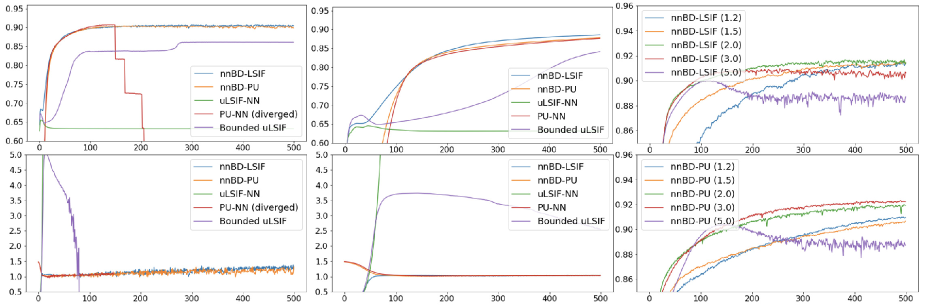
Figure 2: Results of Section 5.1. The horizontal axes represent epochs. Left and center figures: The results under different learning rates, $1\times 10^{-4}$ and $1\times 10^{-5}$, respectively, where the vertical axes of the upper graphs show the AUROCs, and those of the lower graphs show $\hat{\mathbb{E}}_{\mathrm{de}}[\hat{r}(X_{i})]$. Right figure: Results of sensitivity analyses, where the vertical axes show the AUROCs.

4.2 Estimation error bound on $L^{2}$ norm

Next, we derive an estimation error bound for $\hat{r}$ on the $L^{2}$ norm. We aim to derive the standard convergence rate of non-parametric regression; that is, under the appropriate conditions, the order of $\|\hat{r}-r^{*}\|_{L^{2}(p_{\mathrm{de}})}$ is nearly $\mathcal{O}_{\mathbb{P}}\left(1/(n_{\mathrm{de}}\land n_{\mathrm{nu}})\right)$ (Kanamori et al., 2012). Note that unlike the generalization error bound of the BD, we require a stronger assumption on the loss function, namely, a strong convexity. In Theorem 1, for a multilayer perception with ReLU activation function (Definition 3), we derive the convergence rate of the $L^{2}$ distance, which is the same rate as that of the nonparametric regression using the Gaussian kernel and the LSIF loss (Kanamori et al., 2012). This result also corresponds to a faster convergence rate than Theorem 1. The proof is shown in Appendix J. To complement this result, we empirically investigate the estimator error using an artificially generated dataset with the known true density ratio in Section 5.2.

Theorem 2 ($L^{2}$ Convergence rate).

Assume $f$ is $\mu$-strongly convex. Let $\mathcal{H}$ be defined as in Definition 3 and assume $r^{*}=\frac{p_{\mathrm{nu}}}{p_{\mathrm{de}}}\in\mathcal{H}$. In addition, assume the same conditions as Theorem 3. Then, for any $0<\gamma<2$, as $n_{\mathrm{de}},n_{\mathrm{nu}}\to\infty$,

$$\|\hat{r}-r^{*}\|_{L^{2}(p_{\mathrm{de}})}\leq\mathcal{O}_{\mathbb{P}}\left((\min\left\{n_{\mathrm{de}},n_{\mathrm{nu}}\right\})^{-1/(2+\gamma)}\right).$$

This $L^{2}$ distance bound is useful for statistical inference. For example, double/debiased machine learning with cross-fitting proposed by Chernozhukov et al. (2016) allows for semiparametric inference under estimators of nuisance parameters with appropriate convergence rates. By using cross-fitting, Uehara et al. (2020) proposed causal inference under covariate shifts when the convergence rate of the density ratio satisfies an appropriate convergence rate. Further, it is expected to be applied to two-sample homogeneity using neural networks, as in Kanamori et al. (2010).

5 Experiments

We experimentally show how existing DRE methods fail and D3RE succeeds when using neural networks.

Table 2: Results of Section 5.2: MSEs and SDs of DRE using synthetic datasets. The lowest MSE methods are highlighted in bold.

		uLSIF	LSIF-NN	D3RE (nnBD-LSIF)
				$C=0.8$	$C=1$	$C=2$	$C=3$	$C=4$	$C=5$	$C=10$	$C=15$	$C=20$
$\mathrm{dim}=10$	MSE	2.378	1.272	1.750	1.695	1.191	0.964	0.873	0.833	0.948	1.079	1.170
	SD	1.143	0.413	0.570	0.563	0.523	0.487	0.459	0.424	0.370	0.331	0.387
$\mathrm{dim}=20$	MSE	1.684	2.694	1.704	1.646	1.307	1.272	1.337	1.444	2.066	2.697	3.098
	SD	0.372	0.409	0.380	0.368	0.328	0.297	0.283	0.288	0.285	0.346	0.374
$\mathrm{dim}=30$	MSE	1.786	3.724	1.811	1.747	1.488	1.577	1.798	2.019	3.238	4.306	5.432
	SD	0.456	0.460	0.459	0.449	0.411	0.400	0.401	0.379	0.370	0.464	0.543
$\mathrm{dim}=50$	MSE	1.791	8.717	1.817	1.753	1.609	1.818	2.194	2.614	4.848	6.955	8.798
	SD	0.562	1.518	0.571	0.555	0.513	0.503	0.484	0.465	0.488	0.597	0.672
$\mathrm{dim}=100$	MSE	1.723	4.849	1.748	1.693	1.626	1.860	2.226	2.709	5.528	8.605	11.557
	SD	0.574	4.182	0.575	0.571	0.540	0.532	0.495	0.563	0.672	0.790	1.140

Table 3: Average AUROC curve (Mean) with the standard deviation (SD) over $5$ trials of anomaly detection methods. For all datasets, each model was trained on a single class and tested against all other classes. The best result is in bold.

MNIST	uLSIF-NN		nnBD-LSIF		nnBD-PU		nnBD-LSIF		nnBD-PU		Deep SAD		GT
Network	LeNet		LeNet		LeNet		WRN		WRN		LeNet		WRN
Inlier Class	Mean	SD	Mean	SD	Mean	SD	Mean	SD	Mean	SD	Mean	SD	Mean	SD
0	0.999	0.000	0.997	0.000	0.999	0.000	1.000	0.000	1.000	0.000	0.592	0.051	0.963	0.002
1	1.000	0.000	0.999	0.000	1.000	0.000	1.000	0.000	1.000	0.000	0.942	0.016	0.517	0.039
2	0.997	0.001	0.994	0.000	0.997	0.001	1.000	0.000	1.000	0.001	0.447	0.027	0.992	0.001
3	0.997	0.000	0.995	0.001	0.998	0.000	1.000	0.000	1.000	0.000	0.562	0.035	0.974	0.001
4	0.998	0.000	0.997	0.001	0.999	0.000	1.000	0.000	1.000	0.000	0.646	0.015	0.989	0.001

CIFAR-10	uLSIF-NN		nnBD-LSIF		nnBD-PU		nnBD-LSIF		nnBD-PU		Deep SAD		GT
Network	LeNet		LeNet		LeNet		WRN		WRN		LeNet		WRN
Inlier Class	Mean	SD	Mean	SD	Mean	SD	Mean	SD	Mean	SD	Mean	SD	Mean	SD
plane	0.745	0.056	0.934	0.002	0.943	0.001	0.925	0.004	0.923	0.001	0.627	0.066	0.697	0.009
car	0.758	0.078	0.957	0.002	0.968	0.001	0.965	0.002	0.960	0.001	0.606	0.018	0.962	0.003
bird	0.768	0.012	0.850	0.007	0.878	0.004	0.844	0.004	0.858	0.004	0.404	0.006	0.752	0.002
cat	0.745	0.037	0.820	0.003	0.856	0.002	0.810	0.009	0.841	0.002	0.517	0.018	0.727	0.014
deer	0.758	0.036	0.886	0.004	0.909	0.002	0.864	0.008	0.872	0.002	0.704	0.052	0.863	0.014

FMNIST	uLSIF-NN		nnBD-LSIF		nnBD-PU		nnBD-LSIF		nnBD-PU		Deep SAD		GT
Network	LeNet		LeNet		LeNet		WRN		WRN		LeNet		WRN
Inlier Class	Mean	SD	Mean	SD	Mean	SD	Mean	SD	Mean	SD	Mean	SD	Mean	SD
T-shirt/top	0.960	0.005	0.981	0.001	0.985	0.000	0.984	0.001	0.982	0.000	0.558	0.031	0.890	0.007
Trouser	0.961	0.010	0.998	0.000	1.000	0.000	0.998	0.000	0.998	0.000	0.758	0.022	0.974	0.004
Pullover	0.944	0.012	0.976	0.001	0.980	0.001	0.983	0.002	0.972	0.001	0.617	0.046	0.902	0.005
Dress	0.973	0.006	0.986	0.001	0.992	0.000	0.991	0.001	0.986	0.000	0.525	0.038	0.843	0.014
Coat	0.958	0.006	0.978	0.001	0.983	0.000	0.981	0.002	0.974	0.000	0.627	0.029	0.885	0.003

5.1 Experiments with image data

To investigate how D3RE prevents train-loss hacking from occurring, we consider a setting of inlier-based outlier detection. For binary labels $y\in\{-1,+1\}$, we consider training a classifier only from $p(X\mid y=+1)$ and $p(X)$ to find a positive data point in the test data sampled from $p(X)$. The goal is to maximize the area under the receiver operating characteristic (AUROC) curve, which is a criterion often used for anomaly detection, by estimating the density ratio $r^{*}(X)=p(X\mid y=+1)/p(X)$. We construct positive and negative datasets from the CIFAR-10 (Krizhevsky, 2009) dataset with $10$ classes. The positive dataset comprises ‘airplane,’ ‘automobile,’ ‘ship,’ and ‘truck’; the negative dataset comprises ‘bird,’ ‘cat,’ ‘deer,’ ‘dog,’ ‘frog,’ and ‘horse.’ We use $1,000$ positive samples generated from $p(X\mid y=+1)$ and $1,000$ unlabeled samples generated from $p(X)$ to train the models. Then, we calculate the AUROCs using $10,000$ test samples generated from $p(X)$. In this case, it is desirable to set $C<\frac{1}{2}$ because $\frac{p(X\mid y=+1)}{0.5p(X\mid y=+1)+0.5p(X\mid y=-1)}=\frac{1}{0.5+0.5\frac{p(X\mid y=-1)}{p(X\mid y=+1)}}$. For demonstrative purposes, we use a basic CNN architecture from the PyTorch tutorial (Paszke et al., 2019). The details are shown in Appendix D.2. The model is trained by the Adam optimizer (Kingma & Ba, 2015) without a weight decay and with the parameters $(\beta_{1},\beta_{2},\epsilon)$ fixed at the default values of the implementation in PyTorch (Paszke et al., 2019), namely $(0.9,0.999,10^{-8})$.

First, we compare two of the proposed estimators, $\widehat{\mathrm{nnBD}}_{\mathrm{PU}}$ (nnBD-PU) and $\widehat{\mathrm{nnBD}}_{\mathrm{LSIF}}$ (nnBD-LSIF), with two existing estimators, $\widehat{\mathrm{BD}}_{\mathrm{PU}}$ (PU-NN) and $\widehat{\mathrm{BD}}_{\mathrm{LSIF}}$ (uLSIF-NN) with neural networks. We use the logistic loss for PULogLoss. In addition, we conduct an experiment with uLSIF-NN using a naively capped model $\tilde{r}(X)=\min\{r(X),1/C\}$ (Bounded uLSIF). We fix the hyperparameter $C$ at $1/3$. We report the results for two learning rates, $1\times 10^{-4}$ and $1\times 10^{-5}$. We conduct $10$ trials, and report the average AUROCs. We also compute $\hat{\mathbb{E}}_{\mathrm{de}}[\hat{r}(X)]$, which should be close to $1$ when the density ratio is successfully estimated since $\int(p(x|y=+1)/p(X))p(X)dx=1$. These results are shown in the left and center figures in Figure 2. In all cases, the proposed estimators outperform the other methods. We consider that the instabilities of PU-NN and LISF-NN are caused by the unboundedness of the objective function (also see Kiryo et al. (2017), where similar experimental results are reported). The results also demonstrate that naive capping (Bounded uLSIF) fails to prevent train-loss hacking from occurring and leads to suboptimal behavior. As discussed in Sections 2.3 and 3.2, naive capping is insufficient for this problem because an unreasonable model such that $r(X^{\mathrm{de}}_{i})=0$ and $r(X^{\mathrm{nu}}_{j})=1/C$ can still be a minimizer by decreasing one part of the empirical BD, e.g., $\frac{1}{2}\hat{\mathbb{E}}_{\mathrm{de}}\left[r^{2}(X)\right]-\frac{C}{2}\hat{\mathbb{E}}_{\mathrm{nu}}\left[r^{2}(X)\right]=0-\frac{1}{2C}$.

Next, we investigate the sensitivity of D3RE to the hyperparameter $C$. We choose $C$ from $\{1/1.2,1/1.5,1/2.0.1/3.0,1/5.0\}$. The other settings remain unchanged from the previous experiment, where the exact upper bound $\overline{R}$ is $2.0$. The results are shown on the right-hand side of Figure 2. While estimators with $1/C\simeq 2.0$ show a superior performance, the method is robust to the choice of $C$ to a certain extent. Additional experimental results are reported in Appendix F.1.

Note that this experimental setting is similar to that of PU learning (Elkan & Noto, 2008; Kiryo et al., 2017). In PU learning experiments, we mainly consider a binary classification problem, and the class-prior $p(y=+1)$ is given; that is, the goals and the presence of the information are the differences between the experimental settings of inlier-based outlier detection and PU learning. In this paper, we successfully related PU learning methods to DRE. The class-prior in PU learning plays a similar role to the upper bound of $r^{*}$ in DRE.

5.2 Experiments on $L^{2}$ error

We empirically investigate the $L^{2}$ error in the proposed D3RE. We compare our method with the uLSIF. For uLSIF (Kanamori et al., 2009), we use an open-source implementation, which uses a linear-in-parameter model with the Gaussian kernel (Kanamori et al., 2012). For D3RE, we use nnBD-LSIF and $3$-layer perceptron with a ReLU activation function, where the number of the nodes in the middle layer is $100$. We conducted nnBD-LSIF for all $C\in\{0.8,1,2,3,4,5,10,15,20\}$. We also compare these methods with a naively implemented LSIF with a $3$-layer perceptron. Let the dimensions of the domain be $d$ and

$$p_{\mathrm{nu}}(X)=\mathcal{N}(X;\mu^{\mathrm{nu}},I_{d}),\ p_{\mathrm{de}}(X)=\mathcal{N}(X;\mu^{\mathrm{de}},I_{d}),$$

where $\mathcal{N}(X;\mu,\Sigma)$ denotes the multivariate normal distribution with mean $\mu$ and $\Sigma$, $\mu^{\mathrm{nu}}$ and $\mu^{\mathrm{de}}$ are $d$-dimensional vectors $\mu^{\mathrm{nu}}=(1,0,\dots,0)^{\top}$ and $\mu^{\mathrm{de}}=(0,0,\dots,0)^{\top}$, and $I_{d}$ is a $d$-dimensional identity matrix. We fix the sample sizes at $n_{\mathrm{nu}}=n_{\mathrm{de}}=1,000$ and estimate the density ratio using uLSIF, LSIF, and D3RE (nnBD-LSIF). To measure the performance, we use the mean squared error (MSE) and the standard deviation (SD) averaged over $50$ trials. Note that in this setting, we know the true density ratio $r^{*}$. The results are shown in Table 2. The proposed nnBD-LSIF method estimates the density ratio more accurately than the other methods with a lower MSE. In many cases of the results, nnBD-LSIF achieves the best performance at approximately $C=2$. This result implies that we do not need to know the exact $C$ to achieve a high level performance in D3RE.

6 Inlier-based outlier detection

As an application of D3RE, we perform inlier-based outlier detection experiments with benchmark datasets. In addition to CIFAR-10, we use MNIST (LeCun et al., 1998) and fashion-MNIST (FMNIST) (Xiao et al., 2017), both of which have $10$ classes. Hido et al. (2008, 2011) applied the a direct DRE for inlier-based outlier detection; that is, finding outliers in a test set based on a training set consisting only of inliers by using the ratio of training and test data densities as an outlier score. Nam & Sugiyama (2015) and Abe & Sugiyama (2019) proposed using shallow neural networks with DRE to deal with this problem. In relation to the experimental setting of Section 5.1, the problem setting can be seen as a transductive variant of PU learning (Kato et al., 2019).

We follow the setting proposed by Golan & El-Yaniv (2018). There are ten classes in each dataset, MNIST, CIFAR-10, and FMNIST. We use one class as an inlier class and treat all other classes as outliers. For example, in the case of CIFAR-10, there are $5,000$ train data per class. On the other hand, there are $1,000$ test data for each class, which amounts to $1,000$ inlier samples and $9,000$ outlier samples. The AUROC is used as a metric to evaluate whether the outlier class can be detected in the outlier samples. We compare the proposed methods with the benchmark methods of deep semi-supervised anomaly detection (DeepSAD) (Ruff et al., 2020) and geometric transformation (GT) (Golan & El-Yaniv, 2018). The details of each method are shown in Appendix E. To make a fair comparison, we use LeNet and Wide ResNet for D3RE, which are the same neural network architectures as those used in Golan & El-Yaniv (2018) and Ruff et al. (2020). The detailed structures are shown in Appendix D. Owing to the space limitation, some of the experimental results with MNIST, CIFAR-10 and FMNIST is shown in Table 3. The full results are shown in Table 4 in Appendix F.2. In almost all cases, the average AUROCs of the proposed methods are better than those of the existing methods. The largest performance gain is seen in the CIFAR-10, where the mean AUROC is improved by $0.157$ on average between the uLSIF-NN and nnBD-LSIF. Although GT and DeepSAD are designed for different problem setups, to the best of our knowledge, there are no other appropriate state-of-the-art alternatives to these algorithms under this setting.

In Appendix G, we also introduce other applications such as covariate shift adaptation.

Togashi et al. (2021) applied our proposed method to personalized ranking from implicit feedback in a recommender systems. For this task, there are two approaches, pointwise and pairwise, and the former of which is known to be computationally efficient, whereas the latter shows better accuracy than the former. In that study, they reformulated a pointwise approach using the density ratio and also added the essence of the pairwise approach.

7 Conclusion

We proposed a non-negative correction to the empirical BD for DRE. Using the prior knowledge of the upper bound of the density ratio, we can prevent train-loss hacking from occurring when using flexible models. In our theoretical analyses, we provided generalization error bounds for the proposed method. In our experiments, we empirically confirmed the effectiveness of our proposed approach.

Appendix A Details of existing methods for DRE

In this section, we overview examples of DRE methods in the framework of the density ratio matching under BD.

Least Squares Importance Fitting (LSIF).

LSIF minimizes the squared error between a density ratio model $r$ and the true density ratio $r^{*}$ defined as follows (Kanamori et al., 2009):

$$R_{\mathrm{LSIF}}(r)=\mathbb{E}_{\mathrm{de}}[(r(X)-r^{*}(X))^{2}]=\mathbb{E}_{\mathrm{de}}[(r^{*}(X))^{2}]-2\mathbb{E}_{\mathrm{nu}}[r(X)]+\mathbb{E}_{\mathrm{de}}[(r(X))^{2}].$$

In the unconstrained LSIF (uLSIF) (Kanamori et al., 2009), we ignore the first term in the above equation and estimate the density ratio by the following minimization problem:

$$\hat{r}=\operatorname*{arg\,min}_{r\in\mathcal{H}}\left[\frac{1}{2}\hat{\mathbb{E}}_{\mathrm{de}}[(r(X))^{2}]-\hat{\mathbb{E}}_{\mathrm{nu}}[r(X)]+\mathcal{R}(r)\right],$$ (6)

where $\mathcal{R}$ is a regularization term. This empirical risk minimization is equal to minimizing the empirical BD defined in (2) with $f(t)=(t-1)^{2}/2$.

Unnormalized Kullback–Leibler (UKL) divergence and KL Importance Estimation Procedure (KLIEP).

The KL importance estimation procedure (KLIEP) is derived from the unnormalized Kullback–Leibler (UKL) divergence objective (Sugiyama et al., 2008; Nguyen et al., 2010; Tsuboi et al., 2009; Yamada & Sugiyama, 2009; Yamada et al., 2010), which uses $f(t)=t\log(t)-t$. Ignoring the terms which are irrelevant for the optimization, we obtain the unnormalized Kullback–Leibler (UKL) divergence objective (Nguyen et al., 2010; Sugiyama et al., 2012) as

$$\mathrm{BD}_{\mathrm{UKL}}(r)=\mathbb{E}_{\mathrm{de}}\left[r(X)\right]-\mathbb{E}_{\mathrm{nu}}\left[\log\big{(}r(X)\big{)}\right].$$

Directly minimizing UKL is proposed by Nguyen et al. (2010). The KLIEP also solves the same problem with further imposing a constraint that the ratio model $r(X)$ is non-negative for all $X$ and is normalized as

$$\hat{\mathbb{E}}_{\mathrm{de}}\left[r(X)\right]=1.$$

Then, following is the optimization criterion of KLIEP (Sugiyama et al., 2008):

$$\max_{r}\hat{\mathbb{E}}_{\mathrm{nu}}\left[\log\big{(}r(X)\big{)}\right]$$

$$\mathrm{s.t.}\ \hat{\mathbb{E}}_{\mathrm{de}}\left[r(X)\right]=1\ \mathrm{and}\ r(X)\geq 0\ \mathrm{for}\ \mathrm{all}\ X.$$

Logistic Regression (LR).

By using $f(t)=\log(t)-(1+t)\log(1+t)$, we obtain the following BD called the binary Kullback–Leibler (BKL) divergence:

$$\mathrm{BD}_{\mathrm{BKL}}(r)=-\mathbb{E}_{\mathrm{de}}\left[\log\left(\frac{1}{1+r(X)}\right)\right]-\mathbb{E}_{\mathrm{nu}}\left[\log\left(\frac{r(X)}{1+r(X)}\right)\right].$$

This BD is derived from a formulation based on the logistic regression (Hastie et al., 2001; Sugiyama et al., 2011b).

PU Learning with the log loss.

Consider a binary classification problem and let $X$ and $y\in\{\pm 1\}$ be the feature and the label of a sample, respectively. In PU learning, the goal is to train a classifier only using positive data sampled from $p(X\mid y=+1)$, and unlabeled data sampled from $p(X)$ in binary classification (Elkan & Noto, 2008). More precisely, this problem setting of PU learning is called the case-control scenario (Elkan & Noto, 2008; Niu et al., 2016). Let $\mathcal{G}$ be the set of measurable functions from $\mathcal{X}$ to $[\epsilon,1-\epsilon]$, where $\epsilon\in(0,1/2)$ is a small positive value. For a loss function $\ell:\mathbb{R}\times\{\pm 1\}\to{\mathbb{R}^{+}}$, du Plessis et al. (2015) showed that the classification risk of $g\in\mathcal{G}$ in the PU problem setting can be expressed as

$$R_{\mathrm{PU}}(g)=\pi\int\Big{(}\ell(g(X),+1)-\ell(g(X),-1)\Big{)}p(X\mid y=+1)dX+\int\ell(g(X),-1)]p(X)dX.$$ (7)

According to Kato et al. (2019), we can derive the following risk for DRE from the risk for PU learning (7) as follows:

$$\mathrm{BD}_{\mathrm{PU}}(g)=\frac{1}{\overline{R}}\mathbb{E}_{\mathrm{nu}}\left[-\log\left(g(X)\right)+\log\left(1-g(X)\right)\right]-\mathbb{E}_{\mathrm{de}}\left[\log\left(1-g(X)\right)\right],$$

and Kato et al. (2019) showed that $g^{*}=\operatorname*{arg\,min}_{g\in\mathcal{G}}\mathrm{BD}_{\mathrm{PU}}(g)$ satisfies the following:

Proposition 1.

It holds almost everywhere that

$$g^{*}(X)=\begin{cases}1-\varepsilon&(X\notin D_{2}),\\ C\frac{p_{\mathrm{nu}}(X)}{p_{\mathrm{de}}(X)}&(X\in D_{1}\cap D_{2}),\\ \varepsilon&(X\notin D_{1}),\end{cases}$$

where $C=\frac{1}{\overline{R}}$, $D_{1}=\{X\mid Cp_{\mathrm{nu}}(X)\geq\epsilon p_{\mathrm{de}}(X)\}$, and $D_{2}=\{X|Cp_{\mathrm{nu}}(X)\leq(1-\epsilon)p_{\mathrm{de}}(X)\}$.

Using this result, we define the empirical version of $\mathrm{BD}_{\mathrm{PU}}(g)$ as follows:

$$\widehat{\mathrm{BD}}_{\mathrm{PU}}(r^{*}\|r):=C\hat{\mathbb{E}}_{\mathrm{nu}}\left[-\log\big{(}r(X_{i})\big{)}+\log\big{(}1-r(X_{j})\big{)}\right]-\hat{\mathbb{E}}_{\mathrm{de}}\left[\log\big{(}1-r(X_{i})\big{)}\right].$$

To see that this is also a BD minimization method, define $f(t)$ as

$$f(t)=C\log\left(1-t\right)+Ct\left(\log\left(t\right)-\log\left(1-t\right)\right).$$

Then, we have

$$\partial f(t)=-\frac{C}{1-t}+C(\log(t)-\log(1-t))+Ct\left(\frac{1}{t}+\frac{1}{1-t}\right).$$

Therefore, we have

$$\mathrm{BD}_{f}(r):=\mathbb{E}_{\mathrm{de}}\Big{[}\partial f\big{(}r(X_{i})\big{)}r(X_{i})-f\big{(}r(X_{i})\big{)}\Big{]}-\mathbb{E}_{\mathrm{nu}}\Big{[}\partial f\big{(}r(X_{j})\big{)}\Big{]}$$

$$=\mathbb{E}_{\mathrm{de}}\Big{[}-\frac{Cr(X_{i})}{1-r(X_{i})}+Cr(X_{i})(\log(r(X_{i}))-\log(1-r(X_{i})))+Cr^{2}(X_{i})\left(\frac{1}{r(X_{i})}+\frac{1}{1-r(X_{i})}\right)\Big{]}$$

$$\ \ \ -\mathbb{E}_{\mathrm{de}}\Big{[}\log\left(1-r(X_{i})\right)+Cr(X_{i})\left(\log\left(r(X_{i})\right)-\log\left(1-r(X_{i})\right)\right)\Big{]}$$

$$\ \ \ -\mathbb{E}_{\mathrm{nu}}\Big{[}-\frac{C}{1-r(X_{i})}+C(\log(r(X_{i}))-\log(1-r(X_{i})))+Cr(X_{i})\left(\frac{1}{r(X_{i})}+\frac{1}{1-r(X_{i})}\right)\Big{]}$$

$$=\mathbb{E}_{\mathrm{de}}\Big{[}-\frac{Cr(X_{i})}{1-r(X_{i})}+Cr(X_{i})(\log(r(X_{i}))-\log(1-r(X_{i})))+\frac{Cr(X_{i})}{1-r(X_{i})}\Big{]}$$

$$\ \ \ -\mathbb{E}_{\mathrm{de}}\Big{[}\log\left(1-r(X_{i})\right)+Cr(X_{i})\left(\log\left(r(X_{i})\right)-\log\left(1-r(X_{i})\right)\right)\Big{]}$$

$$\ \ \ -\mathbb{E}_{\mathrm{nu}}\Big{[}-\frac{C}{1-r(X_{i})}+C(\log(r(X_{i}))-\log(1-r(X_{i})))+\frac{C}{1-r(X_{i})}\Big{]}$$

$$=\mathbb{E}_{\mathrm{de}}\Big{[}\log\left(1-r(X_{i})\right)\Big{]}-C\mathbb{E}_{\mathrm{nu}}\Big{[}\log(r(X_{i}))-\log(1-r(X_{i}))\Big{]}.$$

Remark 1 (DRE and PU learning).

Menon & Ong (2016) showed that minimizing a proper CPE loss is equivalent to minimizing a BD to the true density ratio, and demonstrated the viability of using existing losses from one problem for the other for CPE and DRE. Kato et al. (2019) pointed out the relation between the PU learning and density ratio estimation and leveraged it to solve a sample selection bias problem in PU learning. In this paper, we introduced the BD with $f(t)=\log\left(1-Ct\right)+Ct\left(\log\left(Ct\right)-\log\left(1-Ct\right)\right)$, inspired by the objective function of PU learning with the log loss. In the terminology of Menon & Ong (2016), this $f$ results in a DRE objective without a link function. In other words, it yields a direct DRE method.

Appendix B Examples of $\tilde{f}$

Here, we show the examples of $\tilde{f}$ such that $\partial f(t)=C\big{(}\partial f(t)t-f(t)\big{)}+\tilde{f}(t)$, where $\tilde{f}(t)$ is bounded from above, and $\partial f(t)t-f(t)+A$ is non-negative.

First, we consider $f(t)=(t-1)^{2}/2$, which results in the LSIF objective. Because $\partial f(t)=t-1$, we have

$$t-1=C\big{(}(t-1)t-(t-1)^{2}/2\big{)}+\tilde{f}(t)$$

$$\Leftrightarrow\tilde{f}(t)=-C\big{(}(t-1)t-(t-1)^{2}/2\big{)}+t-1=-\frac{C}{2}t^{2}+\frac{C}{2}+t-1.$$

The function is a concave quadratic function, therefore it is upper bounded.

Second, we consider $f(t)=t\log(t)-t$, which results in the UKL or KLIEP objective. Because $\partial f(t)=\log(t)$, we have

$$\log(t)=C\big{(}\log(t)t-t\log(t)+t\big{)}+\tilde{f}(t)$$

$$\Leftrightarrow\tilde{f}(t)=-tC+\log(t).$$

We can easily confirm that the function is upper bounded by taking the derivative and finding that $t=1/C$ gives the maximum.

Third, we consider $f(t)=t\log(t)-(1+t)\log(1+t)$, which is used for DRE based on LR or BKL. Because $\partial f(t)=\log(t)-\log(1+t)$, we have

$$\log(t)-\log(1+t)=C\big{(}(\log(t)-\log(1+t))t-t\log(t)+(1+t)\log(1+t)\big{)}+\tilde{f}(t)$$

$$\Leftrightarrow\tilde{f}(t)=-C\big{(}\log(1+t)\big{)}+\log(t)-\log(1+t)=\log\left(\frac{C}{1+t}\right)+\log\left(\frac{t}{1+t}\right).$$

We can easily confirm that the function is upper bounded as the terms involving $t$ always add up to be negative.

Fourth, we consider DRE based on PULog. By setting $f(t)=\log\left(1-t\right)+Ct\left(\log\left(t\right)-\log\left(1-t\right)\right)$, we can obtain the same risk functional introduced in Kiryo et al. (2017).

Appendix C Train-loss hacking problem in PU classification

Here, we introduce the train-loss hacking discussed in the PU learning literature (Kiryo et al., 2017). In a standard binary classification problem, we train a classifier $\psi$ by minimizing the following empirical risk:

$$\frac{1}{n}\sum^{n}_{i=1}\mathbbm{1}[y_{i}=+1]\ell(\psi(X_{i}))+\frac{1}{n}\sum^{n}_{i=1}\mathbbm{1}[y_{i}=-1]\ell(-\psi(X_{i})),$$ (8)

where $y_{i}\in\{\pm 1\}$ is a binary label, $X_{i}$ is a feature, and $\ell$ is a loss function. On the other hand, in PU learning formulated by du Plessis et al. (2015), because we only have positive data $\{(y^{\prime}_{i}=+1,X^{\prime}_{i})\}^{n^{\prime}}_{i=1}$ and unlabeled data $\{(\bm{x^{\prime\prime}}_{j})\}^{n^{\prime\prime}}_{j=1}$, we minimize the following alternative empirical risk:

$$\frac{\pi}{n^{\prime}}\sum^{n^{\prime}}_{i=1}\ell(\psi(X^{\prime}_{i})\underbrace{-\frac{\pi}{n^{\prime}}\sum^{n^{\prime}}_{i=1}\ell(-\psi(X^{\prime}_{i}))}_{\text{Cause of train-loss hacking.}}+\frac{1}{n^{\prime\prime}}\sum^{n^{\prime\prime}}_{j=1}\ell(-\psi(X^{\prime\prime}_{j})),$$ (9)

where $\pi$ is a hyperparameter representing $p(y=+1)$. Note that the empirical risk (9) is unbiased to the population binary classification risk (8) (du Plessis et al., 2015). While the the empirical risk (8) of the standard binary classification is lower bounded under an appropriate choice of $\ell$, the empirical risk (9) of PU learning proposed by du Plessis et al. (2015) is not lower bounded owing to the existence of the second term. Therefore, if a model is sufficiently flexible, we can significantly minimize the empirical risk only by minimizing the second term $-\frac{\pi}{n^{\prime}}\sum^{n^{\prime}}_{i=1}\ell(-\psi(X^{\prime}_{i}))$ without increasing the other terms. Kiryo et al. (2017) proposed non-negative risk correction for avoiding this problem when using neural networks.

Appendix D Network structure used in Sections 5.1 and 6

We explain the structures of neural networks used in the experiments.

D.1 Network structure used in Sections 5.1

In Section 5.1, we used CIFAR-10 datasets. The model was a convolutional net (Springenberg et al., 2015): $(32\times 32\times 3)\mathchar 45\relax C(3\times 6,3)\mathchar 45\relax C(3\times 16,3)\mathchar 45\relax 128\mathchar 45\relax 84\mathchar 45\relax 1$, where the input is a $32\times 32$ RGB image, $C(3\times 6,3)$ indicates that $3$ channels of $3\times 6$ convolutions followed by ReLU is used. This structure has been adopted from the tutorial of Paszke et al. (2019).

D.2 Network structure used in Sections 6

Inlier-based Outlier Detection.

We used the same LeNet-type CNNs proposed in Ruff et al. (2020). In the CNNs, each convolutional module consists of a convolutional layer followed by leaky ReLU activations with leakiness $\alpha=0.1$ and $(2\times 2)$-max-pooling. For MNIST, we employ a CNN with two modules: $(32\times 32\times 3)\mathchar 45\relax C(3\times 32,5)\mathchar 45\relax C(32\times 64,5)\mathchar 45\relax C(64\times 128,5)\mathchar 45\relax 1$. For CIFAR-10 we employ the following architecture: $(32\times 32\times 1)\mathchar 45\relax C(1\times 8,5)\mathchar 45\relax C(8\times 4,5)\mathchar 45\relax 1$ with a batch normalization (Ioffe & Szegedy, 2015) after each convolutional layer.

The WRN architecture was proposed in Zagoruyko & Komodakis (2016) and it is also used in Golan & El-Yaniv (2018). This structure improved the performance of image recognition by decreasing the depth and increasing the width of the residual networks (He et al., 2015). We omit the detailed description of the structure here.

Covariate Shift Adaptation.

We used the $5$-layer perceptron with ReLU activations. The structure is $10000\mathchar 45\relax 1000\mathchar 45\relax 1000\mathchar 45\relax 1000\mathchar 45\relax 1000\mathchar 45\relax 1$.

Figure 3: The learning curves of the experiments in Section 5.1. The horizontal axis is epoch. The vertical axes of the top figures indicate the training losses. The vertical axes of the bottom figures show the AUROC for the test data. The bottom figures are identical to the ones displayed in Section 5.1.

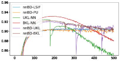
Figure 4: The results of Section F.1.1. The horizontal axis is epoch, and the vertical axis is AUROC.

Appendix E Existing methods for anomaly detection

This section introduces the existing methods for anomaly detection. DeepSAD is a method for semi-supervised anomaly detection, which tries to take advantage of labeled anomalies (Ruff et al., 2020). GT proposed by Golan & El-Yaniv (2018) trains neural networks based on a self-labeled dataset by performing $72$ geometric transformations. The anomaly score based on GT is calculated based on the Dirichlet distribution obtained by maximum likelihood estimation using the softmax output from the trained network.

In the problem setting of the DeepSAD, we have access to a small pool of labeled samples, e.g. a subset verified by some domain expert as being normal or anomalous. In the experimental results shown in Ruff et al. (2020) indicate that, when we can use such samples, the DeepSAD outperforms the other methods. However, in our experimental results, such samples are not assumed to be available, hence the method does not perform well. The problem setting of Ruff et al. (2020) and ours are both termed semi-supervised learning in anomaly detection, but the two settings are different.

Appendix F Details of experiments

The details of experiments are shown in this section. The description of the data is as follows:

MNIST:

The MNIST database is one of the most popular benchmark datasets for image classification, which consists of $28\times 28$ pixel handwritten digits from $0$ to $9$ with $60,000$ train samples and $10,000$ test samples (LeCun et al., 1998). See http://yann.lecun.com/exdb/mnist/.

CIFAR-10:

The CIFAR-10 dataset consists of $60,000$ color images of size $32\times 32$ from $10$ classes, each having $6000$. There are $50,000$ training images and $10,000$ test images (Krizhevsky et al., 2012). See https://www.cs.toronto.edu/~kriz/cifar.html.

fashion-MNIST:

The fashion-MNIST dataset consists of $70,000$ grayscale images of size $28\times 28$ from $10$ classes. There are $60,000$ training images and $10,000$ test images (Xiao et al., 2017). See https://github.com/zalandoresearch/fashion-mnist.

Amazon Review Dataset:

Blitzer et al. (2007) published the text data of Amazon review. The data originally consists of a rating ($0$-$5$ stars) for four different genres of products in the electronic commerce site Amazon.com: books, DVDs, electronics, and kitchen appliances. Blitzer et al. (2007) also released the pre-processed and balanced data of the original data. The pre-processed data consists of text data with four labels $1$, $2$, $4$, and $5$. We map the text data into $10,000$ dimensional data by the TF-IDF mapping with that vocabulary size. In the experiment, for the pre-processed data, we solve the regression problem where the text data are the inputs and the ratings $1$, $2$, $4$, and $5$ are the outputs. When evaluating the performance, following Menon & Ong (2016), we calculate PD (=1-AUROUC) by regarding $4$ and $5$ ratings as positive labels and $1$ and $2$ ratings as negative labels.

F.1 Experiments with image data

We show the additional results of Section 5.1. In Figure 3, we show the training loss of LSIF-based methods to demonstrate the train-loss hacking phenomenon caused by the objective function without a lower bound. In Figure 3, even though the training loss of uLSIF-NN and that of Bounded uLSIF decrease more rapidly than that of nnBD-LSIF, the test AUROC score (the higher the better) either drops or fails to increase. These graphs are the manifestations of the severe train-loss hacking in DRE without our proposed device.

F.1.1 Comparison with various estimators using nnBD divergence

Let UKL-NN and BKL-NN be DRE method with the UKL and BKL losses with neural networks without non-negative correction. Finally, we examine the performances of nnBD-LSIF, nnBD-PU, UKL-NN, BKL-NN, nnBD-UKL, and nnBD-BKL. The learning rate was $1\times 10^{-4}$, and the other settings were identical to those in the previous experiments. These results are shown in Figure 4. UKL-NN and BKL-NN also suffer from train-loss hacking although BKL loss seems to be more robust against the train-loss hacking than the other loss functions. Although nnBD-UKL and nnBD-BKL show better performance in earlier epochs, nnBD-LSIF and nnBD-PU appear to be more stable.

F.1.2 Results without gradient ascent

We also show the experimental results without the gradient ascent heuristic. Figure 5 corresponds to the Figure 2 without the gradient ascent heuristic. Figure 6 corresponds to the Figure 3 without the gradient ascent heuristic. Figure 7 corresponds to the Figure 4 without the gradient ascent heuristic. As shown in these experiments, although the gradient ascent/descent heuristic improve the performance, there is no significant difference between empirical performance with and without the heuristic. Therefore, we recommend practitioners to use the gradient ascent/descent heuristic, but if the reader concerns the theoretical guarantee, they can use the plain gradient descent algorithm; that is, naively minimize the proposed empirical nnBD risk.

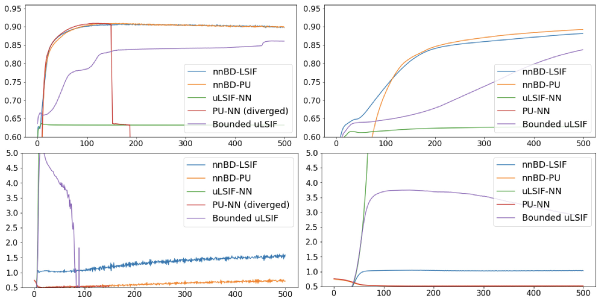
Figure 5: Experimental results of Section 5.1 without gradient ascent/descent heuristic. The horizontal axis is epoch, and the vertical axis is AUROC. The learning rates of the left and right graphs are $1\times 10^{-4}$ and $1\times 10^{-5}$, respectively. The upper graphs show the AUROCs and the lower graphs show $\hat{\mathbb{E}}_{\mathrm{de}}[\hat{r}(X)]$, which will approach $1$ when we successfully estimate the density ratio.

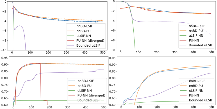
Figure 6: The learning curves of the experiments in Section 5.1 without gradient ascent/descent heuristic. The horizontal axis is epoch. The vertical axes of the top figures indicate the training losses. The vertical axes of the bottom figures show the AUROC for the test data. The bottom figures are identical to the ones displayed in Section 5.1.

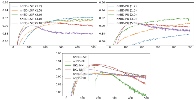
Figure 7: The detailed experimental results for Section F.1.1. The horizontal axis is epoch, and the vertical axis is AUROC.

F.2 Experiments of inlier-based outlier detection

In Table 4, we show the full results of inlier-based outlier detection. In almost all the cases, D3RE for inlier-based outlier detection outperforms the other methods. As explained in Section E, we consider that DeepSAD does not work well because the method assumes the availability of the labeled anomaly data, which is not available in our problem setting.

In Table 5, for different $1/C$ chosen from $\{1,3,5,10\}$, we report the AUROCs of nnBD-LSIF with and without gradient ascent. As shown in the results, loose specification does not significantly decrease the performances. The gradient ascent technique improves the performances, but plain gradient descent still performs well.

Remark 2 (Benchmark Methods).

Although GT is outperformed by our proposed method, the problem setting for the comparison is not in favor of GT as it does not assume the access to the test data. Recently proposed methods for semi-supervised anomaly detection by Ruff et al. (2020) did not perform well without using other side information used in Ruff et al. (2020). On the other hand, there is no other competitive methods in this problem setting, to the best of our knowledge.

F.3 Experiments of covariate shift adaptation

In Table 6, we show the detailed results of experiments of covariate shift adaptation. Even when the training data and the test data follow the same distribution, the covariate shift adaptation based on D3RE improves the mean PD. We consider that this is because the importance weighting emphasizes the loss in the empirical higher-density regions of the test examples.

Table 4: Average area under the ROC curve (Mean) of anomaly detection methods averaged over $5$ trials with the standard deviation (SD). For all datasets, each model was trained on the single class, and tested against all other classes. The best performing method in each experiment is in bold. SD: Standard deviation.

MNIST	uLSIF-NN		nnBD-LSIF		nnBD-PU		nnBD-LSIF		nnBD-PU		Deep SAD		GT
Network	LeNet		LeNet		LeNet		WRN		WRN		LeNet		WRN
Inlier Class	Mean	SD	Mean	SD	Mean	SD	Mean	SD	Mean	SD	Mean	SD	Mean	SD
0	0.999	0.000	0.997	0.000	0.999	0.000	1.000	0.000	1.000	0.000	0.592	0.051	0.963	0.002
1	1.000	0.000	0.999	0.000	1.000	0.000	1.000	0.000	1.000	0.000	0.942	0.016	0.517	0.039
2	0.997	0.001	0.994	0.000	0.997	0.001	1.000	0.000	1.000	0.001	0.447	0.027	0.992	0.001
3	0.997	0.000	0.995	0.001	0.998	0.000	1.000	0.000	1.000	0.000	0.562	0.035	0.974	0.001
4	0.998	0.000	0.997	0.001	0.999	0.000	1.000	0.000	1.000	0.000	0.646	0.015	0.989	0.001
5	0.997	0.000	0.996	0.001	0.998	0.000	1.000	0.000	1.000	0.000	0.502	0.046	0.990	0.001
6	0.997	0.001	0.997	0.001	0.999	0.000	1.000	0.000	1.000	0.000	0.671	0.027	0.998	0.000
7	0.996	0.001	0.993	0.001	0.998	0.001	1.000	0.000	1.000	0.001	0.685	0.032	0.927	0.004
8	0.997	0.000	0.994	0.001	0.997	0.000	0.999	0.000	0.999	0.000	0.654	0.026	0.949	0.002
9	0.993	0.002	0.990	0.002	0.994	0.001	0.998	0.001	0.998	0.001	0.786	0.021	0.989	0.001

CIFAR-10	uLSIF-NN		nnBD-LSIF		nnBD-PU		nnBD-LSIF		nnBD-PU		Deep SAD		GT
Network	LeNet		LeNet		LeNet		WRN		WRN		LeNet		WRN
Inlier Class	Mean	SD	Mean	SD	Mean	SD	Mean	SD	Mean	SD	Mean	SD	Mean	SD
plane	0.745	0.056	0.934	0.002	0.943	0.001	0.925	0.004	0.923	0.001	0.627	0.066	0.697	0.009
car	0.758	0.078	0.957	0.002	0.968	0.001	0.965	0.002	0.960	0.001	0.606	0.018	0.962	0.003
bird	0.768	0.012	0.850	0.007	0.878	0.004	0.844	0.004	0.858	0.004	0.404	0.006	0.752	0.002
cat	0.745	0.037	0.820	0.003	0.856	0.002	0.810	0.009	0.841	0.002	0.517	0.018	0.727	0.014
deer	0.758	0.036	0.886	0.004	0.909	0.002	0.864	0.008	0.872	0.002	0.704	0.052	0.863	0.014
dog	0.728	0.103	0.875	0.004	0.906	0.002	0.887	0.005	0.896	0.002	0.490	0.025	0.873	0.002
frog	0.750	0.060	0.944	0.003	0.958	0.001	0.948	0.004	0.948	0.001	0.744	0.014	0.879	0.008
horse	0.782	0.048	0.928	0.003	0.948	0.002	0.921	0.007	0.927	0.002	0.519	0.015	0.953	0.001
ship	0.780	0.048	0.958	0.003	0.965	0.001	0.964	0.002	0.957	0.001	0.430	0.062	0.921	0.009
truck	0.708	0.081	0.939	0.003	0.955	0.001	0.952	0.003	0.949	0.001	0.393	0.008	0.911	0.003

FMNIST	uLSIF-NN		nnBD-LSIF		nnBD-PU		nnBD-LSIF		nnBD-PU		Deep SAD		GT
Network	LeNet		LeNet		LeNet		WRN		WRN		LeNet		WRN
Inlier Class	Mean	SD	Mean	SD	Mean	SD	Mean	SD	Mean	SD	Mean	SD	Mean	SD
T-shirt/top	0.960	0.005	0.981	0.001	0.985	0.000	0.984	0.001	0.982	0.000	0.558	0.031	0.890	0.007
Trouser	0.961	0.010	0.998	0.000	1.000	0.000	0.998	0.000	0.998	0.000	0.758	0.022	0.974	0.004
Pullover	0.944	0.012	0.976	0.001	0.980	0.001	0.983	0.002	0.972	0.001	0.617	0.046	0.902	0.005
Dress	0.973	0.006	0.986	0.001	0.992	0.000	0.991	0.001	0.986	0.000	0.525	0.038	0.843	0.014
Coat	0.958	0.006	0.978	0.001	0.983	0.000	0.981	0.002	0.974	0.000	0.627	0.029	0.885	0.003
Sandal	0.968	0.011	0.997	0.001	0.999	0.000	0.999	0.000	0.999	0.000	0.681	0.023	0.949	0.005
Shirt	0.919	0.005	0.952	0.001	0.958	0.001	0.944	0.005	0.932	0.001	0.618	0.015	0.842	0.004
Sneaker	0.991	0.001	0.994	0.002	0.998	0.000	0.998	0.000	0.998	0.000	0.802	0.054	0.954	0.006
Bag	0.980	0.005	0.994	0.001	0.999	0.000	0.998	0.000	0.999	0.000	0.447	0.034	0.973	0.006
Ankle boot	0.992	0.001	0.985	0.015	0.999	0.000	0.997	0.000	0.996	0.000	0.583	0.023	0.996	0.000

Table 5: We show average area under the ROC curve (Mean) of anomaly detection methods averaged over $5$ trials with the standard deviation (SD) for nnBD-LSIF with LeNet. We choose $1/C$, which represents a guessed upper bound, from $\{1,3,5,10\}$. Each model is trained on the single class, and tested against all other classes. We show both results with and without gradient ascent and $\circ$ denotes the use of the gradient ascent technique. The best performing method for each inlier class is highlighted in bold. The best performing method for each $1/C$ is highlighted in underline.

CIFAR-10	nnBD-LSIF
Network	LeNet
$1/C$ (Guessed upper bound)	$1$				$3$				$5$				$10$
With gradient ascent	$\circ$				$\circ$				$\circ$				$\circ$
Inlier Class	Mean	SD	Mean	SD	Mean	SD	Mean	SD	Mean	SD	Mean	SD	Mean	SD	Mean	SD
plane	0.491	0.009	0.642	0.019	0.934	0.002	0.918	0.003	0.920	0.003	0.899	0.002	0.886	0.007	0.839	0.009
car	0.521	0.032	0.644	0.011	0.957	0.002	0.950	0.002	0.951	0.003	0.939	0.004	0.920	0.006	0.894	0.013
bird	0.501	0.013	0.622	0.012	0.850	0.007	0.832	0.004	0.835	0.005	0.812	0.006	0.818	0.004	0.765	0.010
cat	0.491	0.015	0.616	0.014	0.820	0.003	0.807	0.003	0.802	0.007	0.770	0.005	0.773	0.011	0.721	0.006
deer	0.523	0.017	0.658	0.022	0.886	0.004	0.879	0.001	0.873	0.005	0.862	0.004	0.852	0.007	0.820	0.009
dog	0.514	0.018	0.621	0.011	0.875	0.004	0.855	0.005	0.852	0.008	0.820	0.007	0.821	0.009	0.758	0.017
frog	0.496	0.018	0.671	0.018	0.944	0.003	0.932	0.003	0.927	0.003	0.917	0.005	0.886	0.004	0.845	0.014
horse	0.506	0.017	0.631	0.018	0.928	0.003	0.910	0.003	0.916	0.005	0.885	0.003	0.880	0.007	0.823	0.020
ship	0.494	0.027	0.680	0.026	0.958	0.003	0.949	0.001	0.956	0.002	0.942	0.002	0.933	0.004	0.907	0.006
truck	0.506	0.013	0.660	0.016	0.939	0.003	0.930	0.003	0.922	0.003	0.907	0.007	0.885	0.007	0.843	0.018

Table 6: Average PD (Mean) with standard deviation (SD) over $10$ trials with different seeds per method. The best performing method in terms of the mean PD is specified by bold face.

Domains (Train $\to$ Test)	books $\to$ books		dvd $\to$ books		dvd $\to$ dvd		elec $\to$ books		elec $\to$ dvd
DRE method	Mean	SD	Mean	SD	Mean	SD	Mean	SD	Mean	SD
w/o IW	0.093	0.003	0.128	0.008	0.100	0.005	0.212	0.012	0.187	0.008
Kernel uLSIF	0.089	0.002	0.114	0.006	0.094	0.004	0.200	0.009	0.179	0.006
Kernel KLIEP	0.089	0.002	0.116	0.006	0.094	0.004	0.205	0.011	0.184	0.008
uLSIF-NN	0.093	0.003	0.128	0.008	0.100	0.005	0.212	0.012	0.187	0.008
PU-NN	0.093	0.003	0.128	0.008	0.100	0.005	0.212	0.012	0.187	0.008
nnBD-LSIF	0.086	0.002	0.113	0.005	0.091	0.004	0.199	0.009	0.176	0.005
nnBD-PU	0.090	0.003	0.113	0.006	0.096	0.004	0.199	0.009	0.176	0.006

Domains (Train $\to$ Test)	elec $\to$ elec		kitchen $\to$ books		kitchen $\to$ dvd		kitchen $\to$ elec		kitchen $\to$ kitchen
DRE method	Mean	SD	Mean	SD	Mean	SD	Mean	SD	Mean	SD
w/o IW	0.079	0.005	0.202	0.013	0.185	0.006	0.073	0.004	0.062	0.002
Kernel uLSIF	0.072	0.003	0.192	0.007	0.178	0.008	0.071	0.003	0.060	0.003
Kernel KLIEP	0.072	0.003	0.195	0.005	0.182	0.007	0.072	0.004	0.060	0.002
uLSIF-NN	0.079	0.005	0.202	0.013	0.185	0.006	0.073	0.004	0.062	0.002
PU-NN	0.079	0.005	0.202	0.013	0.185	0.006	0.073	0.004	0.062	0.002
nnBD-LSIF	0.071	0.003	0.189	0.008	0.174	0.008	0.068	0.003	0.058	0.003
nnBD-PU	0.074	0.004	0.190	0.008	0.174	0.008	0.068	0.003	0.062	0.005

Appendix G Other applications

In this section, we explain other potential applications of the proposed method.

G.1 Covariate shift adaptation by importance weighting

We consider training a model using input distribution different from the test input distribution, which is called covariate shift, (Bickel et al., 2009). To solve this problem, the density ratio has been used via importance weighting (IW) (Shimodaira, 2000; Yamada et al., 2010; Reddi et al., 2015).

We use a document dataset of Amazon (Blitzer et al., 2007) for multi-domain sentiment analysis (Blitzer et al., 2007). This data consists of text reviews from four different product domains: book, electronics (elec), dvd, and kitchen. Following Chen et al. (2012) and Menon & Ong (2016), we transform the text data using TF-IDF to map them into the instance space $\mathcal{X}=\mathbb{R}^{10000}$ (Salton & McGill, 1986). Each review is endowed with four labels indicating the positivity of the review, and our goal is to conduct regression for these labels. To achieve this goal, we perform kernel ridge regression with the polynomial kernel. We compare regression without IW (w/o IW) with regression using the density ratio estimated by PU-NN, uLSIF-NN, nnBD-LSIF, nnBD-PU, uLSIF with Gaussian kernels (Kernel uLSIF), and KLIEP with Gaussian kernels (Kernel KLIEP). We conduct experiments on $2,000$ samples from one domain, and test $2,000$ samples. Following Menon & Ong (2016), we reduce the dimension into $100$ dimensions by principal component analysis when using Kernel uLSIF, Kernel KLEIP, and regressions. Following Menon & Ong (2016) and Cortes & Mohri (2011), the mean and standard deviation of the pairwise disagreement (PD), $1-\mathrm{AUROC}$, is reported. A part of results is in Table 7. The full results are in Appendix F.3. The methods with D3RE show preferable performance, but the improvement is not significant compared with the image data. We consider this is owing to the difficulty of the covariate shift problem in this dataset.

Table 7: Average PD (Mean) with standard deviation (SD) over $10$ trials with different seeds per method. The best performing method in terms of the mean PD is specified by bold face.

Domains (Train $\to$ Test)	book $\to$ dvd		book $\to$ elec		book $\to$ kitchen		dvd $\to$ elec		dvd $\to$ kitchen		elec $\to$ kitchen
DRE method	Mean	SD	Mean	SD	Mean	SD	Mean	SD	Mean	SD	Mean	SD
w/o IW	0.126	0.008	0.174	0.010	0.166	0.009	0.162	0.006	0.146	0.010	0.074	0.005
Kernel uLSIF	0.122	0.009	0.162	0.009	0.159	0.007	0.153	0.006	0.142	0.007	0.068	0.005
Kernel KLIEP	0.130	0.010	0.164	0.009	0.161	0.007	0.154	0.006	0.143	0.006	0.070	0.005
uLSIF-NN	0.126	0.008	0.174	0.010	0.166	0.009	0.162	0.006	0.146	0.010	0.074	0.005
PU-NN	0.126	0.008	0.174	0.010	0.166	0.009	0.162	0.006	0.146	0.010	0.074	0.005
nnBD-LSIF	0.120	0.008	0.160	0.008	0.157	0.008	0.148	0.006	0.138	0.007	0.066	0.005
nnBD-PU	0.119	0.008	0.160	0.008	0.156	0.007	0.148	0.005	0.138	0.007	0.066	0.005

$f$-divergence estimation.

$f$-divergences (Ali & Silvey, 1966; Csiszár, 1967) are the discrepancy measures of probability densities based on the density ratio, hence the proposed method can be used for their estimation. They include the KL divergence (Kullback & Leibler, 1951), the Hellinger distance (Hellinger, 1909), and the Pearson divergence (Pearson, 1900), as examples.

Two-sample homogeneity test.

The purpose of a homogeneity test is to determine if two or more datasets come from the same distribution (Loevinger, 1948). For two-sample testing, using a semiparametric $f$-divergence estimator with nonparametric density ratio models has been studied (Keziou., 2003; Keziou & Leoni-Aubin, 2005). Kanamori et al. (2010) and Sugiyama et al. (2011a) employed direct DRE for the nonparametric DRE.

Generative adversarial networks.

Generative adversarial networks (GANs) are successful deep generative models, which learns to generate new data with the same distribution as the training data Goodfellow et al. (2014). Various GAN methods have been proposed, amongst which Nowozin et al. (2016) proposed f-GAN, which minimizes the variational estimate of $f$-divergence. Uehara et al. (2016) extended the idea of Nowozin et al. (2016) to use BD minimization for DRE. The estimator proposed in this paper also has a potential to improve the method of Uehara et al. (2016).

Average treatment effect estimation and off-policy evaluation.

One of the goals in causal inference is to estimate the expected treatment effect, which is a counterfactual value. Therefore, following the causality formulated by Rubin (1974), we consider estimating the average treatment effect (ATE). Recently, from machine learning community, off-policy evaluation (OPE) is also proposed, which is a generalization of ATE (Dudík et al., 2011; Imai & Ratkovic, 2014; Wang et al., 2017; Narita et al., 2019; Bibaut et al., 2019; Kallus & Uehara, 2019; Oberst & Sontag, 2019). OPE has garnered attention in applications such as advertisement design selection, personalized medicine, search engines, and recommendation systems (Beygelzimer & Langford, 2009; Li et al., 2010; Athey & Wager, 2017).

The problem in ATE estimation and OPE is sample selection bias. For removing the bias, the density ratio has a critical role. An idea of using the density ratio dates back to (Rosenbaum, 1987), which proposed an inverse probability weighting (IPW) method (Horvitz & Thompson, 1952) for ATE estimation. In the IPW method, we approximate the parameter of interest with the sample average with inverse assignment probability of treatment (action), which is also called propensity score. Here, it is known that using the true assignment probability yields higher variance than the case where we use an estimated assignment probability even if we know the true value (Hirano et al., 2003; Henmi & Eguchi, 2004; Henmi et al., 2007). This property can be explained from the viewpoint of semiparametric efficiency (Bickel et al., 1998). While the asymptotic variance of the IPW estimator with an estimated propensity score can achieve the efficiency bound, that of the IPW estimator with the true propensity score does not.

By extending the IPW estimator, more robust ATE estimators are proposed by Rosenbaum (1983), which is known as a doubly robust (DR) estimator. The doubly robust estimator is not only robust to model misspecification but also useful in showing asymptotic normality. In particular, when using the density ratio and the other nuisance parameters estimated from the machine learning method, the conventional IPW and DR estimators do not have asymptotic normality (Chernozhukov et al., 2018). This is because the nuisance estimators do not satisfy Donsker’s condition, which is required for showing the asymptotic normality of semiparametric models. However, by using the sample splitting method proposed by Klaassen (1987), Zheng & van der Laan (2011), and Chernozhukov et al. (2018), we can show the asymptotic normality when using the DR estimator. Note that for the IPW estimator, we cannot show the asymptotic normality even if using sample-splitting.

When using the IPW and DR estimator, we often consider a two-stage approach: in the first stage, we estimate the nuisance parameters, including the density ratio; in the second stage, we construct a semiparametric ATE estimator including the first-stage nuisance estimators. This is also called two-step generalized method of moments (GMM). On the other hand, from the causal inference community, there are also weighting-based covariate balancing methods (Qin & Zhang, 2007; Tan, 2010; Hainmueller, 2012; Imai & Ratkovic, 2014). In particular, Imai & Ratkovic (2014) proposed a covariate balancing propensity score (CBPS), which simultaneously estimates the density ratio and ATE. The idea of CBPS is to construct moment conditions, including the density ratios, and estimate the ATE and density ratio via GMM simultaneously. Although the asymptotic property of the CBPS is the same as other conventional estimators, existing empirical studies report that the CBPS outperforms them (Wyss et al., 2014).

Readers may feel that the CBPS (Imai & Ratkovic, 2014) has a close relationship with the direct DRE, but we consider that it is less relevant to the context of the direct DRE. From the DRE perspective, the method of Imai & Ratkovic (2014) boils down to the method of Gretton et al. (2009), which proposed direct DRE through moment matching. The research motivation of Imai & Ratkovic (2014) is to estimate the ATE with estimating a nuisance density ratio estimator simultaneously. Therefore, the density ratio itself is nuisance parameter; that is, they are not interested in the estimation performance of the density ratio. Under their motivation, they are interested in a density ratio estimator satisfying the moment condition for estimating the ATE, not in a density ratio estimator predicting the true density ratio well. In addition, while the direct DRE method adopts linear-in-parameter models and neural networks (our work), it is not appropriate to use those methods with the CBPS (Chernozhukov et al., 2018). This is because the density ratio estimator does not satisfy Donsker’s condition. Even naive Ridge and Lasso regression estimators do not satisfy the Donsker’s condition. Therefore, when using machine learning methods for estimating the density ratio, we cannot show asymptotic normality of an ATE estimator obtained by the CBPS; therefore, we need to use the sample-splitting method by (Chernozhukov et al., 2018). This means that when using the CBPS, we can only use a naive parametric linear model without regularization or classic nonparametric kernel regression. Recently, for GMM with such non-Donsker nuisance estimators, Chernozhukov et al. (2016) also proposed a new GMM method based on the conventional two-step approach. For these reasons, the CBPS is less relevant to the direct DRE context.

Off-policy evaluation with external validity.

By the problem setting of combining causal inference and domain adaptation, Uehara et al. (2020) recently proposed using covariate shift adaptation to solve the external validity problem in OPE, i.e., the case that the distribution of covariates is the same between the historical and evaluation data (Cole & Stuart, 2010; Pearl & Bareinboim, 2014).

Change point detection.

The methods for change-point detection try to detect abrupt changes in time-series data (Basseville & Nikiforov, 1993; Brodsky & Darkhovsky, 1993; Gustafsson, 2000; Nguyen et al., 2011). There are two types of problem settings in change-point detection, namely the real-time detection (Adams, 2007; Garnett et al., 2009; Paquet, 2007) and the retrospective detection (Basseville & Nikiforov, 1993; Yamanishi & Takeuchi, 2002). In retrospective detection, which requires longer reaction periods, Liu et al. (2012) proposed using techniques of direct DRE. Whereas the existing methods rely on linear-in-parameter models, our proposed method enables us to employ more complex models for change point detection.

Similarity-based sentiment analysis.

Kato (2019) used the density ratio estimated from PU learning for sentiment analysis of text data based on similarity.

Appendix H Generalization error bound

The generalization error bound can be proved by building upon the proof techniques in Kiryo et al. (2017); Lu et al. (2020).

Notations for the theoretical analysis.

We denote the set of real values by $\mathbb{R}$ and that of positive integers by $\mathbb{N}$. Let $\mathcal{X}\subset\mathbb{R}^{d}$. Let $p_{\mathrm{nu}}(x)$ and $p_{\mathrm{de}}(x)$ be probability density functions over $\mathcal{X}$, and assume that the density ratio $r^{*}(x):=\frac{p_{\mathrm{nu}}(x)}{p_{\mathrm{de}}(x)}$ is existent and bounded: $\overline{R}:=\|r^{*}\|_{\infty}<\infty$. Assume $0<C<\frac{1}{\overline{R}}$. Since $\overline{R}\geq 1$ (because $1=\int p_{\mathrm{de}}(x)r^{*}(x)dx\leq 1\cdot\|r^{*}\|_{\infty}$), we have $C\in(0,1]$ and hence $p_{\mathrm{mod}}:=p_{\mathrm{de}}-Cp_{\mathrm{nu}}>0$.

Problem Setup.

Let the hypothesis class of density ratio be $\mathcal{H}\subset\{r:\mathbb{R}^{D}\to(b_{r},B_{r})=:I_{r}\}$, where $0\leq b_{r}<\overline{R}<B_{r}$. Let $f:I_{r}\to\mathbb{R}$ be a twice continuously-differentiable convex function with a bounded derivative. Define $\tilde{f}$ by $\partial f(t)=C(\partial f(t)t-f(t))+\tilde{f}(t)$, where $\partial f$ is the derivative of $f$ continuously extended to $0$ and $B_{r}$. Recall the definitions $\ell_{1}(t):=\partial f(t)t-f(t)+A$, $\ell_{2}(t):=-\tilde{f}(t)$, and

$$\begin{split}\mathrm{BD}_{f}(r)&:=\mathbb{E}_{\mathrm{de}}\left[\partial f(r(X))r(X)-f(r(X))+A\right]-\mathbb{E}_{\mathrm{nu}}\left[\partial f(r(X))\right]\\ &=\mathbb{E}\hat{\mathbb{E}}_{\mathrm{mod}}\left[\partial f(r(X))r(X)-f(r(X))+A\right]-\mathbb{E}_{\mathrm{nu}}\left[\tilde{f}(r(X))\right]\\ &=\mathbb{E}\hat{\mathbb{E}}_{\mathrm{mod}}\ell_{1}(r(X))+\mathbb{E}_{\mathrm{nu}}\ell_{2}(r(X))\\ &\left(=(\mathbb{E}_{\mathrm{de}}-C\mathbb{E}_{\mathrm{nu}})\ell_{1}(r(X))+\mathbb{E}_{\mathrm{nu}}\ell_{2}(r(X))\right),\\ \widehat{\mathrm{nnBD}}_{f}(r)&:=\rho\left(\hat{\mathbb{E}}_{\mathrm{mod}}\ell_{1}(r(X))\right)+\hat{\mathbb{E}}_{\mathrm{nu}}\ell_{2}(r(X))\\ &\left(=\rho((\hat{\mathbb{E}}_{\mathrm{de}}-C\hat{\mathbb{E}}_{\mathrm{nu}})\ell_{1}(r(X))+\hat{\mathbb{E}}_{\mathrm{nu}}\ell_{2}(r(X))\right),\\ \end{split}$$

where we denoted $\hat{\mathbb{E}}_{\mathrm{mod}}=\hat{\mathbb{E}}_{\mathrm{de}}-C\hat{\mathbb{E}}_{\mathrm{nu}}$ and $\rho$ is a consistent correction function with Lipschitz constant $L_{\rho}$ (Definition 1).

Remark 3.

The true density ratio $r^{*}$ minimizes $\mathrm{BD}_{f}$.

Definition 1 (Consistent correction function (Lu et al., 2020)).

A function $f:\mathbb{R}\to\mathbb{R}$ is called a consistent correction function if it is Lipschitz continuous, non-negative and $f(x)=x$ for all $x\geq 0$.

Definition 2 (Rademacher complexity).

Given $n\in\mathbb{N}$ and a distribution $p$, define the Rademacher complexity $\mathcal{R}_{n}^{p}(\mathcal{H})$ of a function class $\mathcal{H}$ as

$$\begin{split}\mathcal{R}_{n}^{p}(\mathcal{H}):=\mathbb{E}_{p}\mathbb{E}_{\sigma}\left[\sup_{r\in\mathcal{H}}\left|\frac{1}{n}\sum_{i=1}^{n}\sigma_{i}r(X_{i})\right|\right],\end{split}$$

where $\{\sigma_{i}\}_{i=1}^{n}$ are Rademacher variables (i.e., independent variables following the uniform distribution over $\{-1,+1\}$) and ${\{X_{i}\}_{i=1}^{n}\overset{\text{i.i.d.}}{\sim}p}$.

The theorem in the paper is a special case of Theorem 3 with $\rho(\cdot):=\max\{0,\cdot\}$ (in which case $L_{\rho}=1$) and Theorem 4.

Theorem 3 (Generalization error bound).

Assume that ${B_{\ell}}:=\sup_{t\in I_{r}}\{\max\{|\ell_{1}(t)|,|\ell_{2}(t)|\}\}<\infty$. Assume $\ell_{1}$ is $L_{\ell_{1}}$-Lipschitz and $\ell_{2}$ is $L_{\ell_{2}}$-Lipschitz. Assume that there exists an empirical risk minimizer $\hat{r}\in\operatorname*{arg\,min}_{r\in\mathcal{H}}\widehat{\mathrm{nnBD}}_{f}(r)$ and a population risk minimizer $\bar{r}\in\operatorname*{arg\,min}_{r\in\mathcal{H}}\mathrm{BD}_{f}(r)$. Also assume $\inf_{r\in\mathcal{H}}\mathbb{E}\hat{\mathbb{E}}_{\mathrm{mod}}\ell_{1}(r(X))>0$ and that $(\rho-\mathrm{Id})$ is $(L_{\rho-\mathrm{Id}})$-Lipschitz. Then for any $\delta\in(0,1)$, with probability at least $1-\delta$, we have

$$\begin{split}\mathrm{BD}_{f}(\hat{r})-\mathrm{BD}_{f}(\bar{r})&\leq 8L_{\rho}L_{\ell_{1}}\mathcal{R}_{n_{\mathrm{de}}}^{p_{\mathrm{de}}}(\mathcal{H})+8(L_{\rho}CL_{\ell_{1}}+L_{\ell_{2}})\mathcal{R}_{n_{\mathrm{nu}}}^{p_{\mathrm{nu}}}(\mathcal{H})\\ &\qquad+2\Phi_{(C,f,\rho)}(n_{\mathrm{nu}},n_{\mathrm{de}})+{B_{\ell}}\sqrt{8\left(\frac{L_{\rho}^{2}}{n_{\mathrm{de}}}+\frac{(1+L_{\rho}C)^{2}}{n_{\mathrm{nu}}}\right)\log\frac{1}{\delta}},\end{split}$$

where $\Phi_{(C,f,\rho)}(n_{\mathrm{nu}},n_{\mathrm{de}})$ is defined as in Lemma 2.

Proof.

Since $\hat{r}$ minimizes $\widehat{\mathrm{nnBD}}_{f}$, we have

$$\begin{split}\mathrm{BD}_{f}(\hat{r})-\mathrm{BD}_{f}(\bar{r})&=\mathrm{BD}_{f}(\hat{r})-\widehat{\mathrm{nnBD}}_{f}(\hat{r})+\widehat{\mathrm{nnBD}}_{f}(\hat{r})-\mathrm{BD}_{f}(\bar{r})\\ &\leq\mathrm{BD}_{f}(\hat{r})-\widehat{\mathrm{nnBD}}_{f}(\hat{r})+\widehat{\mathrm{nnBD}}_{f}(\bar{r})-\mathrm{BD}_{f}(\bar{r})\\ &\leq 2\sup_{r\in\mathcal{H}}|\widehat{\mathrm{nnBD}}_{f}(r)-\mathrm{BD}_{f}(r)|\\ &\leq\underbrace{2\sup_{r\in\mathcal{H}}|\widehat{\mathrm{nnBD}}_{f}(r)-\mathbb{E}\widehat{\mathrm{nnBD}}_{f}(r)|}_{\text{Maximal deviation}}+\underbrace{2\sup_{r\in\mathcal{H}}|\mathbb{E}\widehat{\mathrm{nnBD}}_{f}(r)-\mathrm{BD}_{f}(r)|}_{\text{Bias}}.\end{split}$$

We apply McDiarmid’s inequality (McDiarmid, 1989; Mohri et al., 2018) to the maximal deviation term. The absolute value of the difference caused by altering one data point in the maximal deviation term is bounded from above by $2{B_{\ell}}\frac{L_{\rho}}{n_{\mathrm{de}}}$ if the altered point is a sample from $p_{\mathrm{de}}$ and $2{B_{\ell}}\frac{1+L_{\rho}C}{n_{\mathrm{nu}}}$ if it is from $p_{\mathrm{nu}}$. Therefore, McDiarmid’s inequality implies, with probability at least $1-\delta$, that we have

$$\sup_{r\in\mathcal{H}}|\widehat{\mathrm{nnBD}}_{f}(r)-\mathbb{E}\widehat{\mathrm{nnBD}}_{f}(r)|$$

$$\quad\leq\underbrace{\mathbb{E}\left[\sup_{r\in\mathcal{H}}|\widehat{\mathrm{nnBD}}_{f}(r)-\mathbb{E}\widehat{\mathrm{nnBD}}_{f}(r)|\right]}_{\text{Expected maximal deviation}}+{B_{\ell}}\sqrt{2\left(\frac{L_{\rho}^{2}}{n_{\mathrm{de}}}+\frac{(1+L_{\rho}C)^{2}}{n_{\mathrm{nu}}}\right)\log\frac{1}{\delta}}.$$

Applying Lemma 1 to the expected maximal deviation term and Lemma 2 to the bias term, we obtain the assertion. ∎

The following lemma generalizes the symmetrization lemmas proved in Kiryo et al. (2017) and Lu et al. (2020).

Lemma 1 (Symmetrization under Lipschitz-continuous modification).

Let $0\leq a<b$, $J\in\mathbb{N}$, and $\{K_{j}\}_{j=1}^{J}\subset\mathbb{N}$. Given i.i.d. samples $\mathcal{D}_{(j,k)}:=\{X_{i}\}_{i=1}^{n_{(j,k)}}$ each from a distribution $p_{(j,k)}$ over $\mathcal{X}$, consider a stochastic process $\hat{S}$ indexed by $\mathcal{F}\subset(a,b)^{\mathcal{X}}$ of the form

$$\begin{split}\hat{S}(f)=\sum_{j=1}^{J}\rho_{j}\left(\sum_{k=1}^{K_{j}}\hat{\mathbb{E}}_{(i,j)}[\ell_{(j,k)}(f(X))]\right),\end{split}$$

where each $\rho_{j}$ is a $L_{\rho_{j}}$-Lipschitz function on $\mathbb{R}$, $\ell_{(j,k)}$ is a $L_{\ell_{(j,k)}}$-Lipschitz function on $(a,b)$, and $\hat{\mathbb{E}}_{(i,j)}$ denotes the expectation with respect to the empirical measure of $\mathcal{D}_{(j,k)}$. Denote $S(f):=\mathbb{E}\hat{S}(f)$ where $\mathbb{E}$ is the expectation with respect to the product measure of $\{\mathcal{D}_{(j,k)}\}_{(j,k)}$. Here, the index $j$ denotes the grouping of terms due to $\rho_{j}$, and $k$ denotes each sample average term. Then we have

$$\begin{split}\mathbb{E}\sup_{f\in\mathcal{F}}|\hat{S}(f)-S(f)|\leq 4\sum_{j=1}^{J}\sum_{k=1}^{K_{j}}L_{\rho_{j}}L_{\ell_{(j,k)}}\mathcal{R}_{n_{(j,k)},p_{(j,k)}}(\mathcal{F}).\end{split}$$

Proof.

First, we consider a continuous extension of $\ell_{(j,k)}$ defined on $(a,b)$ to $[0,b)$. Since the functions in $\mathcal{F}$ take values only in $(a,b)$, this extension can be performed without affecting the values of $\hat{S}(f)$ or $S(f)$. We extend the function by defining the values for $x\in[0,a]$ as $\ell_{(j,k)}(x):=\lim_{x^{\prime}\downarrow a}\ell_{(j,k)}(x^{\prime})$, where the right-hand side is guaranteed to exist since $\ell_{(j,k)}$ is Lipschitz continuous hence uniformly continuous. Then, $\ell_{(j,k)}$ remains a $L_{\rho_{j}}$-Lipschitz continuous function on $[0,b)$. Now we perform symmetrization (Vapnik, 1998), deal with $\rho_{j}$’s, and then bound the symmetrized process by Rademacher complexity. Denoting independent copies of $\{X_{(j,k)}\}$ by $\{X^{(\mathrm{gh})}_{j,k}\}_{(j,k)}$ and the corresponding expectations as well as the sample averages with ^(gh),

$$\begin{split}&\mathbb{E}\sup_{f\in\mathcal{F}}|\hat{S}(f)-S(f)|\\ &\leq\sum_{j=1}^{J}\mathbb{E}\sup_{f\in\mathcal{F}}|\rho_{j}(\sum_{k=1}^{K_{j}}\hat{\mathbb{E}}_{(i,j)}\ell_{(j,k)}(f(X)))-\mathbb{E}^{(\mathrm{gh})}\rho_{j}(\sum_{k=1}^{K_{j}}\hat{\mathbb{E}}^{(\mathrm{gh})}_{(j,k)}\ell_{(j,k)}(f(X^{(\mathrm{gh})})))|\\ &\leq\sum_{j=1}^{J}\mathbb{E}\mathbb{E}^{(\mathrm{gh})}\sup_{f\in\mathcal{F}}|\rho_{j}(\sum_{k=1}^{K_{j}}\hat{\mathbb{E}}_{(i,j)}\ell_{(j,k)}(f(X)))-\rho_{j}(\sum_{k=1}^{K_{j}}\hat{\mathbb{E}}^{(\mathrm{gh})}_{(j,k)}\ell_{(j,k)}(f(X^{(\mathrm{gh})})))|\\ &\leq\sum_{j=1}^{J}L_{\rho_{j}}\sum_{k=1}^{K_{j}}\mathbb{E}\mathbb{E}^{(\mathrm{gh})}\sup_{f\in\mathcal{F}}|\hat{\mathbb{E}}_{(i,j)}\ell_{(j,k)}(f(X))-\hat{\mathbb{E}}^{(\mathrm{gh})}_{(j,k)}\ell_{(j,k)}(f(X^{(\mathrm{gh})}))|\\ &=\sum_{j=1}^{J}L_{\rho_{j}}\sum_{k=1}^{K_{j}}\mathbb{E}\mathbb{E}^{(\mathrm{gh})}\sup_{f\in\mathcal{F}}|\hat{\mathbb{E}}_{(i,j)}(\ell_{(j,k)}(f(X))-\ell_{(j,k)}(0))-\hat{\mathbb{E}}^{(\mathrm{gh})}_{(j,k)}(\ell_{(j,k)}(f(X^{(\mathrm{gh})}))-\ell_{(j,k)}(0))|\\ &\leq\sum_{j=1}^{J}L_{\rho_{j}}\sum_{k=1}^{K_{j}}\left(2\mathcal{R}_{n_{(j,k)},p_{(j,k)}}(\{\ell_{(j,k)}\circ f-\ell_{(j,k)}(0):f\in\mathcal{F}\})\right)\\ &\leq\sum_{j=1}^{J}L_{\rho_{j}}\sum_{k=1}^{K_{j}}2\cdot 2L_{\ell_{(j,k)}}\mathcal{R}_{n_{(j,k)},p_{(j,k)}}(\mathcal{F}),\end{split}$$

where we applied Talagrand’s contraction lemma for two-sided Rademacher complexity (Ledoux & Talagrand, 1991; Bartlett & Mendelson, 2001) with respect to $(t\mapsto\ell_{(j,k)}(t)-\ell_{(j,k)}(0))$ in the last inequality. ∎

Lemma 2 (Bias due to risk correction).

Assume $\inf_{r\in\mathcal{H}}\mathbb{E}\hat{\mathbb{E}}_{\mathrm{mod}}\ell_{1}(r(X))>0$ and that $(\rho-\mathrm{Id})$ is $(L_{\rho-\mathrm{Id}})$-Lipschitz on $\mathbb{R}$. There exists $\alpha>0$ such that

$$\begin{split}\sup_{r\in\mathcal{H}}|\mathbb{E}\widehat{\mathrm{nnBD}}_{f}(r)-\mathrm{BD}_{f}(r)|&\leq(1+C){B_{\ell}}L_{\rho-\mathrm{Id}}\exp\left(-\frac{2\alpha^{2}}{({B_{\ell}}^{2}/n_{\mathrm{de}})+(C^{2}{B_{\ell}}^{2}/n_{\mathrm{nu}})}\right)\\ &=:\Phi_{(C,f,\rho)}(n_{\mathrm{nu}},n_{\mathrm{de}}).\end{split}$$

Remark 4.

Note that we already have $p_{\mathrm{mod}}\geq 0$ and $\ell_{1}\geq 0$ and hence $\inf_{r\in\mathcal{H}}\mathbb{E}\hat{\mathbb{E}}_{\mathrm{mod}}\ell_{1}(r(X))\geq 0$. Therefore, the assumption of Lemma 2 is essentially referring to the strict positivity of the infimum. Here, $\mathbb{E}\hat{\mathbb{E}}_{\mathrm{mod}}$ and $\mathbb{P}\left(\cdot\right)$ denote the expectation and the probability with respect to the joint distribution of the samples included in $\hat{\mathbb{E}}_{\mathrm{mod}}$.

Proof.

Fix an arbitrary $r\in\mathcal{H}$. We have

$$|\mathbb{E}\widehat{\mathrm{nnBD}}_{f}(r)-\mathrm{BD}_{f}(r)|=|\mathbb{E}[\widehat{\mathrm{nnBD}}_{f}(r)-\widehat{\mathrm{BD}}_{f}(r)]|$$

$$=|\mathbb{E}[\rho(\hat{\mathbb{E}}_{\mathrm{mod}}\ell_{1}(r(X)))-\hat{\mathbb{E}}_{\mathrm{mod}}\ell_{1}(r(X))]|\leq\mathbb{E}\left[|\rho(\hat{\mathbb{E}}_{\mathrm{mod}}\ell_{1}(r(X)))-\hat{\mathbb{E}}_{\mathrm{mod}}\ell_{1}(r(X))|\right]$$

$$=\mathbb{E}\left[\mathbbm{1}\{\rho(\hat{\mathbb{E}}_{\mathrm{mod}}\ell_{1}(r(X)))\neq\hat{\mathbb{E}}_{\mathrm{mod}}\ell_{1}(r(X))\}\cdot|\rho(\hat{\mathbb{E}}_{\mathrm{mod}}\ell_{1}(r(X)))-\hat{\mathbb{E}}_{\mathrm{mod}}\ell_{1}(r(X))|\right]$$

$$\leq\mathbb{E}\left[\mathbbm{1}\{\rho(\hat{\mathbb{E}}_{\mathrm{mod}}\ell_{1}(r(X)))\neq\hat{\mathbb{E}}_{\mathrm{mod}}\ell_{1}(r(X))\}\right]\left(\sup_{s:|s|\leq(1+C){B_{\ell}}}|\rho(s)-s|\right)$$

where $\mathbbm{1}\{\cdot\}$ denotes the indicator function, and we used $|\hat{\mathbb{E}}_{\mathrm{mod}}\ell_{1}(r(X))|\leq(1+C){B_{\ell}}$. Further, we have

$$\sup_{s:|s|\leq(1+C){B_{\ell}}}|\rho(s)-s|\leq\sup_{s:|s|\leq(1+C){B_{\ell}}}|(\rho-\mathrm{Id})(s)-(\rho-\mathrm{Id})(0)|+|(\rho-\mathrm{Id})(0)|$$

$$\leq\sup_{s:|s|\leq(1+C){B_{\ell}}}L_{\rho-\mathrm{Id}}|s-0|+0\leq(1+C){B_{\ell}}L_{\rho-\mathrm{Id}},$$

where $\mathrm{Id}$ denotes the identity function. On the other hand, since $\inf_{r\in\mathcal{H}}\mathbb{E}\hat{\mathbb{E}}_{\mathrm{mod}}\ell_{1}(r(X))>0$ is assumed, there exists $\alpha>0$ such that for any $r\in\mathcal{H}$, $\mathbb{E}\hat{\mathbb{E}}_{\mathrm{mod}}\ell_{1}(r(X))>\alpha$. Therefore, denoting the support of a function by $\mathrm{supp}(\cdot)$,

$$\mathbb{E}\left[\mathbbm{1}\{\rho(\hat{\mathbb{E}}_{\mathrm{mod}}\ell_{1}(r(X)))\neq\hat{\mathbb{E}}_{\mathrm{mod}}\ell_{1}(r(X))\}\right]=\mathbb{P}\left(\hat{\mathbb{E}}_{\mathrm{mod}}\ell_{1}(r(X))\in\mathrm{supp}(\rho-\mathrm{Id})\right)$$

$$\leq\mathbb{P}\left(\hat{\mathbb{E}}_{\mathrm{mod}}\ell_{1}(r(X))<0\right)\leq\mathbb{P}\left(\hat{\mathbb{E}}_{\mathrm{mod}}\ell_{1}(r(X))<\mathbb{E}\hat{\mathbb{E}}_{\mathrm{mod}}\ell_{1}(r(X))-\alpha\right)$$

holds. Now we apply McDiarmid’s inequality to the right-most quantity. The absolute difference caused by altering one data point in $\hat{\mathbb{E}}_{\mathrm{mod}}\ell_{1}(r(X))$ is bounded by $\frac{{B_{\ell}}}{n_{\mathrm{de}}}$ if the change is in a sample from $p_{\mathrm{de}}$ and $\frac{C{B_{\ell}}}{n_{\mathrm{nu}}}$ otherwise. Therefore, McDiarmid’s inequality implies

$$\begin{split}\mathbb{P}\left(\hat{\mathbb{E}}_{\mathrm{mod}}\ell_{1}(r(X))<\mathbb{E}\hat{\mathbb{E}}_{\mathrm{mod}}\ell_{1}(r(X))-\alpha\right)\leq\exp\left(-\frac{2\alpha^{2}}{({B_{\ell}}^{2}/n_{\mathrm{de}})+(C^{2}{B_{\ell}}^{2}/n_{\mathrm{nu}})}\right).\\ \end{split}$$

∎

Theorem 4 (Generalization error bound).

Under Assumption 3, for any $\delta\in(0,1)$, with probability at least $1-\delta$, we have $\mathrm{BD}_{f}(\hat{r})-\mathrm{BD}_{f}(\bar{r})\leq L_{\ell_{1}}\mathcal{R}_{n_{\mathrm{de}}}^{p_{\mathrm{de}}}(\mathcal{H})+8(CL_{\ell_{1}}+L_{\ell_{2}})\mathcal{R}_{n_{\mathrm{nu}}}^{p_{\mathrm{nu}}}(\mathcal{H})+2\Phi_{C}^{f}(n_{\mathrm{nu}},n_{\mathrm{de}})+{B_{\ell}}\sqrt{8\left(\frac{1}{n_{\mathrm{de}}}+\frac{(1+C)^{2}}{n_{\mathrm{nu}}}\right)\log\frac{1}{\delta}}$, where $\Phi_{C}^{f}(n_{\mathrm{nu}},n_{\mathrm{de}}):=(1+C){B_{\ell}}\exp\left(-\frac{2\alpha^{2}}{({B_{\ell}}^{2}/n_{\mathrm{de}})+(C^{2}{B_{\ell}}^{2}/n_{\mathrm{nu}})}\right)$ and $\alpha>0$ is a constant determined in the proof of Lemma 2 in Appendix H.

Remark 5 (Explicit form of the bound in Theorem 1).

Here, we show the explicit form of the bound in Theorem 1 as follows:

$$\mathrm{BD}_{f}(\hat{r})-\mathrm{BD}_{f}(\bar{r})$$

$$\leq\frac{\kappa_{1}}{\sqrt{n_{\mathrm{de}}}}+\frac{\kappa_{2}}{\sqrt{n_{\mathrm{nu}}}}+2\Phi_{C}^{f}(n_{\mathrm{nu}},n_{\mathrm{de}})+{B_{\ell}}\sqrt{8\left(\frac{1}{n_{\mathrm{de}}}+\frac{(1+C)^{2}}{n_{\mathrm{nu}}}\right)\log\frac{1}{\delta}}$$

$$=L_{\ell_{1}}\frac{B_{p_{\mathrm{de}}}\left(\sqrt{2\log(2)L}+1\right)\prod_{j=1}^{L}B_{W_{j}}}{\sqrt{n_{\mathrm{de}}}}$$

$$\ \ \ +8(CL_{\ell_{1}}+L_{\ell_{2}})\frac{B_{p_{\mathrm{nu}}}\left(\sqrt{2\log(2)L}+1\right)\prod_{j=1}^{L}B_{W_{j}}}{\sqrt{n_{\mathrm{nu}}}}$$

$$\ \ \ +2(1+C){B_{\ell}}\exp\left(-\frac{2\alpha^{2}}{({B_{\ell}}^{2}/n_{\mathrm{de}})+(C^{2}{B_{\ell}}^{2}/n_{\mathrm{nu}})}\right)$$

$$\ \ \ +{B_{\ell}}\sqrt{8\left(\frac{1}{n_{\mathrm{de}}}+\frac{(1+C)^{2}}{n_{\mathrm{nu}}}\right)\log\frac{1}{\delta}}.$$

Appendix I Rademacher complexity bound

The following lemma provides an upper-bound on the Rademacher complexity for multi-layer perceptron models in terms of the Frobenius norms of the parameter matrices. Alternatively, other approaches to bound the Rademacher complexity can be employed. The assertion of the lemma follows immediately from the proof of Theorem 1 of Golowich et al. (2019) after a slight modification to incorporate the absolute value function in the definition of Rademacher complexity.

Lemma 3 (Rademacher complexity bound (Golowich et al., 2019, Theorem 1)).

Assume the distribution $p$ has a bounded support: $B_{p}:=\sup_{x\in\mathrm{supp}(p)}\|x\|<\infty$. Let $\mathcal{H}$ be the class of real-valued networks of depth $L$ over the domain $\mathcal{X}$, where each parameter matrix $W_{j}$ has Frobenius norm at most $B_{W_{j}}\geq 0$, and with $1$-Lipschitz activation functions $\varphi_{j}$ which are positive-homogeneous (i.e., $\varphi_{j}$ is applied element-wise and $\varphi_{j}(\alpha t)=\alpha\varphi_{j}(t)$ for all $\alpha\geq 0$). Then

$$\begin{split}\mathcal{R}_{n}^{p}(\mathcal{H})\leq\frac{B_{p}\left(\sqrt{2\log(2)L}+1\right)\prod_{j=1}^{L}B_{W_{j}}}{\sqrt{n}}.\end{split}$$

Proof.

The assertion immediately follows once we modify the beginning of the proof of Theorem 1 by introducing the absolute value function inside the supremum of the Rademacher complexity as

$$\begin{split}\mathbb{E}_{\sigma}\left[\sup_{r\in\mathcal{H}}\left|\sum_{i=1}^{n}\sigma_{i}r(x_{i})\right|\right]\leq\frac{1}{\lambda}\log\mathbb{E}_{\sigma}\sup_{r\in\mathcal{H}}\exp\left(\lambda\left|\sum_{i=1}\sigma_{i}r(x_{i})\right|\right).\end{split}$$

for $\lambda>0$. The rest of the proof is identical to that of Theorem 1 of Golowich et al. (2019). ∎

Appendix J Proof of Theorem 2

We consider relating the $L^{2}$ error bound to the BD generalization error bound in the following lemma.

Lemma 4 ($L^{2}$ distance bound).

Let $\mathcal{H}:=\{r:\mathcal{X}\to(b_{r},B_{r})=:I_{r}|\int|r(x)|^{2}{\mathrm{d}\bm{x}}<\infty\}$ and assume $r^{*}\in\mathcal{H}$. If $\inf_{t\in I_{r}}f^{\prime\prime}(t)>0$, then there exists $\mu>0$ such that for all $r\in\mathcal{H}$,

$$\begin{split}\|r-r^{*}\|_{L^{2}(p_{\mathrm{de}})}^{2}\leq\frac{2}{\mu}\left(\mathrm{BD}_{f}(r)-\mathrm{BD}_{f}(r^{*})\right)\end{split}$$

holds.

Proof.

Since $\mu:=\inf_{t\in I_{r}}f^{\prime\prime}(t)>0$, the function $f$ is $\mu$-strongly convex. By the definition of strong convexity,

$$\mathrm{BD}_{f}(r)-\mathrm{BD}_{f}(r^{*})=(\mathrm{BD}_{f}(r)-\mathbb{E}_{\mathrm{de}}f(r^{*}(X)))-\underbrace{(\mathrm{BD}_{f}(r^{*})+\mathbb{E}_{\mathrm{de}}f(r^{*}(X)))}_{\text{$=0$}}$$

$$=\mathbb{E}_{\mathrm{de}}\left[f(r^{*}(X))-f(r(X))+\partial f(r(X))(r^{*}(X)-r(X))\right]$$

$$\geq\mathbb{E}_{\mathrm{de}}\left[\frac{\mu}{2}(r^{*}(X)-r(X))^{2}\right]=\frac{\mu}{2}\|r^{*}-r\|_{L^{2}(p_{\mathrm{de}})}^{2}.$$

∎

Lemma 5 ($\ell_{2}$ distance bound).

Fix $r\in\mathcal{H}$. Given $n$ samples $\{x_{i}\}_{i=1}^{n}$ from $p_{\mathrm{de}}$, with probability at least $1-\delta$, we have

$$\begin{split}\frac{1}{n}\sum_{i=1}^{n}(r(x_{i})-r^{*}(x_{i}))^{2}\leq\underbrace{\mathbb{E}\left[(r-r^{*})^{2}(X)\right]}_{\text{$=\|r-r^{*}\|_{L^{2}(p_{\mathrm{de}})}^{2}$}}+(2\overline{R})^{2}\sqrt{\frac{\log\frac{1}{\delta}}{2n}}.\end{split}$$

Proof.

The assertion follows from McDiarmid’s inequality after noting that altering one sample results in an absolute change bounded by $\frac{1}{n}(2\overline{R})^{2}$. ∎

Thus, a generalization error bound in terms of $\mathrm{BD}_{f}$ can be converted to that of an $L^{2}$ distance when the true density ratio and the density ratio model are square-integrable and $f$ is strongly convex. However, when using the result of Theorem 1, the convergence rate shown here is slower than $\mathcal{O}_{\mathbb{P}}\left((\min\left\{n_{\mathrm{de}},n_{\mathrm{nu}}\right\})^{-1/(4)}\right)$. On the other hand, Kanamori et al. (2012) derived $\mathcal{O}_{\mathbb{P}}\left((\min\left\{n_{\mathrm{de}},n_{\mathrm{nu}}\right\})^{-1/(2+\gamma)}\right)$ convergence rate. To derive this bound when using neural network, we need to restrict the neural network models. In the following part, we prove Theorem 2 for the following hypothesis class $\mathcal{H}$.

Definition 3 (ReLU neural networks; Schmidt-Hieber, 2020).

For $L\in\mathbb{N}$ and $p=(p_{0},\ldots,p_{L+1})\in\mathbb{N}^{L+2}$,

$$\mathcal{F}(L,p):= \{f:x\mapsto W_{L}\sigma_{v_{L}}W_{L-1}\sigma_{v_{L-1}}\cdots W_{1}\sigma_{v_{1}}W_{0}x:$$

$$\qquad\qquad W_{i}\in\mathbb{R}^{p_{i+1}\times p_{i}},v_{i}\in\mathbb{R}^{p_{i}}(i=0,\ldots,L)\},$$

where $\sigma_{v}(y):=\sigma(y-v)$, and $\sigma(\cdot)=\max\{\cdot,0\}$ is applied in an element-wise manner. Then, for $s\in\mathbb{N},F\geq 0,L\in\mathbb{N}$, and $p\in\mathbb{N}^{L+2}$, define

$$\mathcal{H}(L,p,s,F):=\{f\in\mathcal{F}(L,p):\sum_{j=0}^{L}\|W_{j}\|_{0}+\|v_{j}\|_{0}\leq s,\|f\|_{\infty}\leq F\},$$

where $\|\cdot\|_{0}$ denotes the number of non-zero entries of the matrix or the vector, and $\|\cdot\|_{\infty}$ denotes the supremum norm. Now, fixing $\bar{L},\bar{p},s\in\mathbb{N}$ as well as $F>0$, we define

$$\mathrm{Ind}_{\bar{L},\bar{p}}:=\{(L,p):L\in\mathbb{N},L\leq\bar{L},p\in[\bar{p}]^{L+2}\},$$

and we consider the hypothesis class

$$\bar{\mathcal{H}} :=\bigcup_{(L,p)\in\mathrm{Ind}_{\bar{L},\bar{p}}}\mathcal{H}(L,p,s,F)$$

$$\mathcal{H} :=\{r\in\bar{\mathcal{H}}:\mathrm{Im}(r)\subset(b_{r},B_{r})\}.$$

Moreover, we define $I_{1}:\mathrm{Ind}_{\bar{L},\bar{p}}\to\mathbb{R}$ and $I:\mathcal{H}\to[0,\infty)$ by

$$I_{1}(L,p) :=2|\mathrm{Ind}_{\bar{L},\bar{p}}|^{\frac{1}{s+1}}(L+1)V^{2},$$

$$I(r) :=\max\left\{\|r\|_{\infty},\min_{\stackrel{{\scriptstyle(L,p)\in\mathrm{Ind}_{\bar{L},\bar{p}}}}{{r\in\mathcal{H}(L,p,s,F)}}}I_{1}(L,p)\right\},$$

where $V:=\prod_{l=0}^{L+1}(p_{l}+1)$, and we define

$$\mathcal{H}_{M}:=\{r\in\mathcal{H}:I(r)\leq M\}.$$

Note that the requirement for the hypothesis class of Theorem 1 is not as tight as that of Theorem 2. Then, we prove Theorem 2 as follows:

Proof.

Thanks to the strong convexity, by Lemma 4, we have

$$\frac{\mu}{2}\|\hat{r}-r^{*}\|_{L^{2}(p_{\mathrm{de}})}^{2}\leq\mathrm{BD}_{f}(\hat{r})-\mathrm{BD}_{f}(r^{*})$$

$$=\mathrm{BD}_{f}(\hat{r})-\mathrm{BD}_{f}(r^{*})$$

$$\qquad\underbrace{-\widehat{\mathrm{BD}}_{f}(\hat{r})+\widehat{\mathrm{BD}}_{f}(\hat{r})}_{\text{$=0$}}\underbrace{-\widehat{\mathrm{nnBD}}_{f}(\hat{r})+\widehat{\mathrm{nnBD}}_{f}(\hat{r})}_{\text{$=0$}}\underbrace{-\widehat{\mathrm{BD}}_{f}(r^{*})+\widehat{\mathrm{BD}}_{f}(r^{*})}_{\text{$=0$}}$$

$$\leq\mathrm{BD}_{f}(\hat{r})-\widehat{\mathrm{BD}}_{f}(\hat{r})+(\widehat{\mathrm{BD}}_{f}(\hat{r})-\widehat{\mathrm{nnBD}}_{f}(\hat{r}))$$

$$\qquad+(\widehat{\mathrm{nnBD}}_{f}(r^{*})-\widehat{\mathrm{BD}}_{f}(r^{*}))+\widehat{\mathrm{BD}}_{f}(r^{*})-\mathrm{BD}_{f}(r^{*})$$

$$\leq\underbrace{(\mathrm{BD}_{f}(\hat{r})-\mathrm{BD}_{f}(r^{*})+\widehat{\mathrm{BD}}_{f}(r^{*})-\widehat{\mathrm{BD}}_{f}(\hat{r}))}_{\text{$=:A$}}+\underbrace{2\sup_{r\in\mathcal{H}}{}|\widehat{\mathrm{BD}}_{f}(r)-\widehat{\mathrm{nnBD}}_{f}(r)|}_{\text{$=:B$}},$$

where we used $\widehat{\mathrm{nnBD}}_{f}(\hat{r})\leq\widehat{\mathrm{nnBD}}_{f}(r^{*})$. To bound $A$, for ease of notation, let $\ell_{1}^{r}=\ell_{1}(r(X))$ and $\ell_{2}^{r}=\ell_{2}(r(X))$. Then, since

$$\mathrm{BD}_{f}(r) =\mathbb{E}_{\mathrm{de}}\ell_{1}(r(X))-C\mathbb{E}_{\mathrm{nu}}\ell_{1}(r(X))+\mathbb{E}_{\mathrm{nu}}\ell_{2}(r(X)),$$

$$\widehat{\mathrm{BD}}_{f}(r) =\hat{\mathbb{E}}_{\mathrm{de}}\ell_{1}(r(X))-C\hat{\mathbb{E}}_{\mathrm{nu}}\ell_{1}(r(X))+\hat{\mathbb{E}}_{\mathrm{nu}}\ell_{2}(r(X)),$$

we have

$$A=\mathrm{BD}_{f}(\hat{r})-\mathrm{BD}_{f}(r^{*})+\widehat{\mathrm{BD}}_{f}(r^{*})-\widehat{\mathrm{BD}}_{f}(\hat{r})$$

$$=(\mathbb{E}_{\mathrm{de}}-\hat{\mathbb{E}}_{\mathrm{de}})(\ell_{1}^{\hat{r}}-\ell_{1}^{r^{*}})-C(\mathbb{E}_{\mathrm{nu}}-\hat{\mathbb{E}}_{\mathrm{nu}})(\ell_{1}^{\hat{r}}-\ell_{1}^{r^{*}})+(\mathbb{E}_{\mathrm{nu}}-\hat{\mathbb{E}}_{\mathrm{nu}})(\ell_{2}^{\hat{r}}-\ell_{2}^{r^{*}})$$

$$\leq|(\mathbb{E}_{\mathrm{de}}-\hat{\mathbb{E}}_{\mathrm{de}})(\ell_{1}^{\hat{r}}-\ell_{1}^{r^{*}})|+C|(\mathbb{E}_{\mathrm{nu}}-\hat{\mathbb{E}}_{\mathrm{nu}})(\ell_{1}^{\hat{r}}-\ell_{1}^{r^{*}})|+|(\mathbb{E}_{\mathrm{nu}}-\hat{\mathbb{E}}_{\mathrm{nu}})(\ell_{2}^{\hat{r}}-\ell_{2}^{r^{*}})|$$

By applying Lemma 10, for any $0<\gamma<2$, we have

$$A\leq\mathcal{O}_{\mathbb{P}}\left(\max\left\{\frac{\|\hat{r}-r^{*}\|_{L^{2}(p_{\mathrm{de}})}^{1-\gamma/2}}{\sqrt{\min\left\{n_{\mathrm{de}},n_{\mathrm{nu}}\right\}}},\frac{1}{(\min\left\{n_{\mathrm{de}},n_{\mathrm{nu}}\right\})^{2/(2+\gamma)}}\right\}\right).$$

On the other hand, by Lemma 12 and Lemma 7, and the assumption $\inf_{r\in\mathcal{H}}\mathbb{E}\hat{\mathbb{E}}_{\mathrm{mod}}\ell_{1}(r(X))>0$, there exists $\alpha>0$ such that we have $B\leq\mathcal{O}_{\mathbb{P}}\left(\exp\left(-\frac{2\alpha^{2}}{({B_{\ell}}^{2}/n_{\mathrm{de}})+(C^{2}{B_{\ell}}^{2}/n_{\mathrm{nu}})}\right)\right)$. Combining the above bounds on $A$ and $B$, for any $0<\gamma<2$, we get

$$\|\hat{r}-r^{*}\|_{L^{2}(p_{\mathrm{de}})}^{2} \leq\mathcal{O}_{\mathbb{P}}\left(\max\left\{\frac{\|\hat{r}-r^{*}\|_{L^{2}(p_{\mathrm{de}})}^{1-\gamma/2}}{\sqrt{\min\left\{n_{\mathrm{de}},n_{\mathrm{nu}}\right\}}},\frac{1}{(\min\left\{n_{\mathrm{de}},n_{\mathrm{nu}}\right\})^{2/(2+\gamma)}}\right\}\right)$$

$$\qquad\qquad+\mathcal{O}_{\mathbb{P}}\left(\exp\left(-\frac{2\alpha^{2}}{({B_{\ell}}^{2}/n_{\mathrm{de}})+(C^{2}{B_{\ell}}^{2}/n_{\mathrm{nu}})}\right)\right)$$

$$\leq\mathcal{O}_{\mathbb{P}}\left(\max\left\{\frac{\|\hat{r}-r^{*}\|_{L^{2}(p_{\mathrm{de}})}^{1-\gamma/2}}{\sqrt{\min\left\{n_{\mathrm{de}},n_{\mathrm{nu}}\right\}}},\frac{1}{(\min\left\{n_{\mathrm{de}},n_{\mathrm{nu}}\right\})^{2/(2+\gamma)}}\right\}\right).$$

As a result, we have

$$\|\hat{r}-r^{*}\|_{L^{2}(p_{\mathrm{de}})}\leq\mathcal{O}_{\mathbb{P}}\left((\min\left\{n_{\mathrm{de}},n_{\mathrm{nu}}\right\})^{-\frac{1}{2+\gamma}}\right).$$

∎

Each lemma used in the proof is provided as follows.

J.1 Complexity of the hypothesis class

For the function classes in Definition 3, we have the following evaluations of their complexities.

Lemma 6 (Lemma 5 in Schmidt-Hieber (2020)).

For $L\in\mathbb{N}$ and $p\in\mathbb{N}^{L+2}$, let $V:=\prod_{l=0}^{L+1}(p_{l}+1)$. Then, for any $\delta>0$,

$$\log\mathcal{N}(\delta,\mathcal{H}(L,p,s,\infty),\|\cdot\|_{\infty})\leq(s+1)\log(2\delta^{-1}(L+1)V^{2}).$$

Lemma 7.

There exists $c>0$ such that

$$\mathcal{R}_{n_{\mathrm{nu}}}^{p_{\mathrm{nu}}}(\mathcal{H})\leq cn_{\mathrm{nu}}^{-1/2},\quad\mathcal{R}_{n_{\mathrm{de}}}^{p_{\mathrm{de}}}(\mathcal{H})\leq cn_{\mathrm{de}}^{-1/2}.$$

Proof.

By Dudley’s entropy integral bound (Wainwright, 2019, Theorem 5.22) and Lemma 6, we have

$$\mathcal{R}_{n_{\mathrm{nu}}}^{p_{\mathrm{nu}}}(\mathcal{H}(L,p,s,F)) \leq 32\int_{0}^{2F}\sqrt{\frac{\log\mathcal{N}(\delta,\mathcal{H}(L,p,s,F),\|\cdot\|_{\infty})}{n_{\mathrm{nu}}}}d\delta$$

$$=\left(32\int_{0}^{2F}\left((s+1)\log(2\delta^{-1}(L+1)V^{2})\right)^{1/2}d\delta\right)n_{\mathrm{nu}}^{-1/2}.$$

Therefore, there exists $c>0$ such that

$$\mathcal{R}_{n_{\mathrm{nu}}}^{p_{\mathrm{nu}}}(\mathcal{H})\leq\sum_{(L,p)\in\mathrm{Ind}_{\bar{L},\bar{p}}}\mathcal{R}_{n_{\mathrm{nu}}}^{p_{\mathrm{nu}}}(\mathcal{H}(L,p,s,F))\leq cn_{\mathrm{nu}}^{-1/2}.$$

The same argument applies to $\mathcal{R}_{n_{\mathrm{de}}}^{p_{\mathrm{de}}}(\mathcal{H})$, and we obtain the assertion. ∎

Lemma 8.

There exists $c_{0}>0$ such that for any $\gamma>0$, any $\delta>0$, and any $M\geq 1$, we have

$$\log\mathcal{N}\left(\delta,\mathcal{H}_{M},\|\cdot\|_{\infty}\right) \leq\frac{s+1}{\gamma}\left(\frac{M}{\delta}\right)^{\gamma}.$$

and

$$\sup_{r\in\mathcal{H}_{M}}\|r-r^{*}\|_{\infty} \leq c_{0}M.$$

Proof.

The first assertion is a result of the following calculation:

$$\log\mathcal{N}\left(\delta,\mathcal{H}_{M},\|\cdot\|_{\infty}\right) \leq\log\sum_{\stackrel{{\scriptstyle(L,p)\in\mathrm{Ind}_{\bar{L},\bar{p}}}}{{I_{1}(L,p)\leq M}}}\mathcal{N}\left(\delta,\mathcal{H}(L,p,s,M),\|\cdot\|_{\infty}\right)$$

$$\leq\log\sum_{\stackrel{{\scriptstyle(L,p)\in\mathrm{Ind}_{\bar{L},\bar{p}}}}{{I_{1}(L,p)\leq M}}}\left(\frac{2}{\delta}(L+1)V^{2}\right)^{s+1}$$

$$\leq\log|\mathrm{Ind}_{\bar{L},\bar{p}}|\left(\frac{1}{\delta}M|\mathrm{Ind}_{\bar{L},\bar{p}}|^{-\frac{1}{s+1}}\right)^{s+1}$$

$$=(s+1)\log\left(\frac{M}{\delta}\right)<(s+1)\frac{1}{\gamma}\left(\frac{M}{\delta}\right)^{\gamma},$$

where the first inequality follows from $\mathcal{H}_{M}\subset\bigcup_{(L,p)\in\mathrm{Ind}_{\bar{L},\bar{p}}:I_{1}(L,p)\leq M}\mathcal{H}(L,p,s,F)$, and the last inequality from $\gamma\log x^{\frac{1}{\gamma}}=\log x<x$ that holds for all $x,\gamma>0$.

The second assertion can be confirmed by noting that for any $r\in\mathcal{H}_{M}$ with $M\geq 1$,

$$\|r-r^{*}\|_{\infty} \leq\|r\|_{\infty}+\|r^{*}\|_{\infty}\leq M+\|r^{*}\|_{\infty}$$

$$\leq\left(1+\frac{\|r^{*}\|_{\infty}}{M}\right)M\leq(1+\|r^{*}\|_{\infty})M$$

holds.

∎

Definition 4 (Derived function class and bracketing entropy).

Given a real-valued function class $\mathcal{F}$, define $\ell\circ\mathcal{F}:=\{\ell\circ f:f\in\mathcal{F}\}$. By extension, we define $I:\ell\circ\mathcal{H}\to[1,\infty)$ by $I(\ell\circ r)=I(r)$ and $\ell\circ\mathcal{H}_{M}:=\{\ell\circ r:r\in\mathcal{H}_{M}\}$. Note that, as a result, $\ell\circ\mathcal{H}_{M}$ coincides with $\{\ell\circ r\in\ell\circ\mathcal{H}:I(\ell\circ r)\leq M\}$.

Lemma 9.

Let $\ell:(b_{r},B_{r})\to\mathbb{R}$ be a $\nu$-Lipschitz continuous function. Let $H_{B}\left(\delta,\mathcal{F},\|\cdot\|_{L^{2}(P)}\right)$ denote the bracketing entropy of $\mathcal{F}$ with respect to a distribution $P$. Then, for any distribution $P$, any $\gamma>0$, any $M\geq 1$, and any $\delta>0$, we have

$$H_{B}\left(\delta,\ell\circ\mathcal{H}_{M},\|\cdot\|_{L^{2}(P)}\right) \leq\frac{(s+1)(2\nu)^{\gamma}}{\gamma}\left(\frac{M}{\delta}\right)^{\gamma}.$$

Moreover, there exists $c_{0}>0$ such that for any $M\geq 1$ and any distribution $P$,

$$\sup_{\ell\circ r\in\ell\circ\mathcal{H}_{M}}\|\ell\circ r-\ell\circ r^{*}\|_{L^{2}(P)} \leq c_{0}\nu M,$$

$$\sup_{\stackrel{{\scriptstyle\ell\circ r\in\ell\circ\mathcal{H}_{M}}}{{\|\ell\circ r-\ell\circ r^{*}\|_{L^{2}(P)}\leq\delta}}}\|\ell\circ r-\ell\circ r^{*}\|_{\infty} \leq c_{0}\nu M,\quad\text{for all }\delta>0.$$

Proof.

By combining Lemma 2.1 in van de Geer (2000) with Lemma 6, we have

$$H_{B}\left(\delta,\ell\circ\mathcal{H}_{M},\|\cdot\|_{L^{2}(P)}\right) \leq\log\mathcal{N}\left(\frac{\delta}{2},\ell\circ\mathcal{H}_{M},\|\cdot\|_{\infty}\right),$$

$$\leq\log\mathcal{N}\left(\frac{\delta}{2\nu},\mathcal{H}_{M},\|\cdot\|_{\infty}\right)\leq\frac{s+1}{\gamma}\left(\frac{2\nu M}{\delta}\right)^{\gamma}.$$

For $M\geq 1$, we have

$$\sup_{\ell\circ r\in\ell\circ\mathcal{H}_{M}}\|\ell\circ r-\ell\circ r^{*}\|_{L^{2}(P)} \leq\sup_{\ell\circ r\in\ell\circ\mathcal{H}_{M}}\|\ell\circ r-\ell\circ r^{*}\|_{\infty}$$

$$\sup_{\stackrel{{\scriptstyle\ell\circ r\in\ell\circ\mathcal{H}_{M}}}{{\|\ell\circ r-\ell\circ r^{*}\|_{L^{2}(P)}\leq\delta}}}\|\ell\circ r-\ell\circ r^{*}\|_{\infty} \leq\sup_{\ell\circ r\in\ell\circ\mathcal{H}_{M}}\|\ell\circ r-\ell\circ r^{*}\|_{\infty},$$

and Lemma 6 implies

$$\sup_{\ell\circ r\in\ell\circ\mathcal{H}_{M}}\|\ell\circ r-\ell\circ r^{*}\|_{\infty}\leq\sup_{r\in\mathcal{H}_{M}}\nu\|r-r^{*}\|_{\infty}\leq\nu c_{0}M.$$

∎

J.2 Bounding the empirical deviations

Lemma 10.

Under the conditions of Theorem 2, for any $0<\gamma<2$, we have

$$|(\mathbb{E}_{\mathrm{de}}-\hat{\mathbb{E}}_{\mathrm{de}})(\ell_{1}^{\hat{r}}-\ell_{1}^{r^{*}})| =\mathcal{O}_{\mathbb{P}}\left(\max\left\{\frac{\|\hat{r}-r^{*}\|_{L^{2}(p_{\mathrm{de}})}^{1-\gamma/2}}{\sqrt{n_{\mathrm{de}}}},\frac{1}{n_{\mathrm{de}}^{2/(2+\gamma)}}\right\}\right)$$

$$|(\mathbb{E}_{\mathrm{nu}}-\hat{\mathbb{E}}_{\mathrm{nu}})(\ell_{1}^{\hat{r}}-\ell_{1}^{r^{*}})| =\mathcal{O}_{\mathbb{P}}\left(\max\left\{\frac{\|\hat{r}-r^{*}\|_{L^{2}(p_{\mathrm{de}})}^{1-\gamma/2}}{\sqrt{n_{\mathrm{nu}}}},\frac{1}{n_{\mathrm{nu}}^{2/(2+\gamma)}}\right\}\right)$$

$$|(\mathbb{E}_{\mathrm{nu}}-\hat{\mathbb{E}}_{\mathrm{nu}})(\ell_{2}^{\hat{r}}-\ell_{2}^{r^{*}})| =\mathcal{O}_{\mathbb{P}}\left(\max\left\{\frac{\|\hat{r}-r^{*}\|_{L^{2}(p_{\mathrm{de}})}^{1-\gamma/2}}{\sqrt{n_{\mathrm{nu}}}},\frac{1}{n_{\mathrm{nu}}^{2/(2+\gamma)}}\right\}\right)$$

as $n_{\mathrm{nu}},n_{\mathrm{de}}\to\infty$.

Proof.

Since $0<\gamma<2$, we can apply Lemma 11 in combination with Lemma 9 to obtain

$$\sup_{r\in\mathcal{H}}\frac{|(\mathbb{E}_{\mathrm{de}}-\hat{\mathbb{E}}_{\mathrm{de}})(\ell_{1}^{r}-\ell_{1}^{r^{*}})|}{D_{1}(r)} =\mathcal{O}_{\mathbb{P}}\left(1\right),$$

$$\sup_{r\in\mathcal{H}}\frac{|(\mathbb{E}_{\mathrm{nu}}-\hat{\mathbb{E}}_{\mathrm{nu}})(\ell_{1}^{r}-\ell_{1}^{r^{*}})|}{D_{2}(r)} =\mathcal{O}_{\mathbb{P}}\left(1\right),$$

$$\sup_{r\in\mathcal{H}}\frac{|(\mathbb{E}_{\mathrm{nu}}-\hat{\mathbb{E}}_{\mathrm{nu}})(\ell_{2}^{r}-\ell_{2}^{r^{*}})|}{D_{3}(r)} =\mathcal{O}_{\mathbb{P}}\left(1\right),$$

where

$$D_{1}(r) =\max\left\{\frac{\|\ell_{1}^{r}-\ell_{1}^{r^{*}}\|_{L^{2}(p_{\mathrm{de}})}^{1-\gamma/2}I(\ell_{1}^{r})^{\gamma/2}}{\sqrt{n_{\mathrm{de}}}},\frac{I(\ell_{1}^{r})}{n_{\mathrm{de}}^{2/(2+\gamma)}}\right\},$$

$$D_{2}(r) =\max\left\{\frac{\|\ell_{1}^{r}-\ell_{1}^{r^{*}}\|_{L^{2}(p_{\mathrm{nu}})}^{1-\gamma/2}I(\ell_{1}^{r})^{\gamma/2}}{\sqrt{n_{\mathrm{nu}}}},\frac{I(\ell_{1}^{r})}{n_{\mathrm{nu}}^{2/(2+\gamma)}}\right\},$$

$$D_{3}(r) =\max\left\{\frac{\|\ell_{2}^{r}-\ell_{2}^{r^{*}}\|_{L^{2}(p_{\mathrm{nu}})}^{1-\gamma/2}I(\ell_{2}^{r})^{\gamma/2}}{\sqrt{n_{\mathrm{nu}}}},\frac{I(\ell_{2}^{r})}{n_{\mathrm{nu}}^{2/(2+\gamma)}}\right\},$$

Noting that $\sup_{r\in\mathcal{H}}I(r)<\infty$, that $\ell_{2},\ell_{1}$ are Lipschitz continuous, and that $\|\hat{r}-r^{*}\|_{L^{2}(p_{\mathrm{nu}})}\leq\left(\sup_{x\in\mathcal{X}}\left|\frac{p_{\mathrm{nu}}(x)}{p_{\mathrm{de}}(x)}\right|\right)\|\hat{r}-r^{*}\|_{L^{2}(p_{\mathrm{de}})}$ holds, we have the assertion. ∎

Following is a proposition originally presented in van de Geer (2000), which was rephrased in Kanamori et al. (2012) in a form that is convenient for our purpose.

Lemma 11 (Lemma 5.14 in van de Geer (2000), Proposition 1 in Kanamori et al. (2012)).

Let $\mathcal{F}\subset L^{2}(P)$ be a function class and the map $I(f)$ be a complexity measure of $f\in\mathcal{F}$, where $I$ is a non-negative function on $\mathcal{F}$ and $I(f_{0})<\infty$ for a fixed $f_{0}\in\mathcal{F}$. We now define $\mathcal{F}_{M}=\{f\in\mathcal{F}:I(f)\leq M\}$ satisfying $\mathcal{F}=\bigcup_{M\geq 1}\mathcal{F}_{M}$. Suppose that there exist $c_{0}>0$ and $0<\gamma<2$ such that

$$\sup_{f\in\mathcal{F}_{M}}\|f-f_{0}\|\leq c_{0}M,\ \sup_{\stackrel{{\scriptstyle f\in\mathcal{F}_{M}}}{{\|f-f_{0}\|_{L^{2}(P)}\leq\delta}}}\|f-f_{0}\|_{\infty}\leq c_{0}M,\quad\text{for all }\delta>0,$$

and that $H_{B}(\delta,\mathcal{F}_{M},P)=\mathcal{O}\left(M/\delta\right)^{\gamma}$. Then, we have

$$\sup_{f\in\mathcal{F}}\frac{\left|\int(f-f_{0})d(P-P_{n})\right|}{D(f)}=\mathcal{O}_{\mathbb{P}}\left(1\right),\ (n\to\infty),$$

where $D(f)$ is defined by

$$D(f)=\max\left\{\frac{\|f-f_{0}\|_{L^{2}(P)}^{1-\gamma/2}I(f)^{\gamma/2}}{\sqrt{n}},\frac{I(f)}{n^{2/(2+\gamma)}}\right\}.$$

J.3 Bounding the difference of the BD estimators

Lemma 12.

Assume $\mathcal{R}_{n_{\mathrm{de}}}^{p_{\mathrm{de}}}(\mathcal{H})=\mathchoice{{\scriptstyle\mathcal{O}}}{{\scriptstyle\mathcal{O}}}{{\scriptscriptstyle\mathcal{O}}}{\scalebox{0.6}{$\scriptscriptstyle\mathcal{O}$}}{}(1)(n_{\mathrm{de}}\to\infty)$ and $\mathcal{R}_{n_{\mathrm{nu}}}^{p_{\mathrm{nu}}}(\mathcal{H})=\mathchoice{{\scriptstyle\mathcal{O}}}{{\scriptstyle\mathcal{O}}}{{\scriptscriptstyle\mathcal{O}}}{\scalebox{0.6}{$\scriptscriptstyle\mathcal{O}$}}{}(1)(n_{\mathrm{nu}}\to\infty)$. Also assume the same conditions as Theorem 3. Then,

$$\sup_{r\in\mathcal{H}}{}|\widehat{\mathrm{nnBD}}_{f}(r)-\widehat{\mathrm{BD}}_{f}(r)|=\mathcal{O}_{\mathbb{P}}\left(\exp\left(-\frac{2\alpha^{2}}{({B_{\ell}}^{2}/n_{\mathrm{de}})+(C^{2}{B_{\ell}}^{2}/n_{\mathrm{nu}})}\right)\right)$$

as $n_{\mathrm{nu}},n_{\mathrm{de}}\to\infty$.

Proof.

First, by combining Lemma 13, the assumption on the Rademacher complexities, and Markov’s inequality, there exist $\alpha>0$ and $n_{\mathrm{de}}^{0},n_{\mathrm{nu}}^{0}\in\mathbb{N}$ such that for any $n_{\mathrm{de}}\geq n_{\mathrm{de}}^{0}$ and $n_{\mathrm{nu}}\geq n_{\mathrm{nu}}^{0}$ and any $\delta\in(0,1)$, we have with probability at least $1-\delta$,

$$\sup_{r\in\mathcal{H}}{}|\widehat{\mathrm{nnBD}}_{f}(r)-\widehat{\mathrm{BD}}_{f}(r)|\leq\frac{(1+C){B_{\ell}}L_{\rho-\mathrm{Id}}}{\delta}\exp\left(-\frac{2\alpha^{2}}{({B_{\ell}}^{2}/n_{\mathrm{de}})+(C^{2}{B_{\ell}}^{2}/n_{\mathrm{nu}})}\right){}.$$

Therefore, we have the assertion. ∎

Lemma 13.

Assume $\mathcal{R}_{n_{\mathrm{de}}}^{p_{\mathrm{de}}}(\mathcal{H})=\mathchoice{{\scriptstyle\mathcal{O}}}{{\scriptstyle\mathcal{O}}}{{\scriptscriptstyle\mathcal{O}}}{\scalebox{0.6}{$\scriptscriptstyle\mathcal{O}$}}{}(1)(n_{\mathrm{de}}\to\infty)$ and $\mathcal{R}_{n_{\mathrm{nu}}}^{p_{\mathrm{nu}}}(\mathcal{H})=\mathchoice{{\scriptstyle\mathcal{O}}}{{\scriptstyle\mathcal{O}}}{{\scriptscriptstyle\mathcal{O}}}{\scalebox{0.6}{$\scriptscriptstyle\mathcal{O}$}}{}(1)(n_{\mathrm{nu}}\to\infty)$. Also assume the same conditions as Theorem 3. Then, there exist $\alpha>0$ and $n_{\mathrm{de}}^{0},n_{\mathrm{nu}}^{0}\in\mathbb{N}$ such that for any $n_{\mathrm{de}}\geq n_{\mathrm{de}}^{0}$ and $n_{\mathrm{nu}}\geq n_{\mathrm{nu}}^{0}$,

$$\mathbb{E}\left[\sup_{r\in\mathcal{H}}{}|\widehat{\mathrm{nnBD}}_{f}(r)-\widehat{\mathrm{BD}}_{f}(r)|\right]\leq(1+C){B_{\ell}}L_{\rho-\mathrm{Id}}\exp\left(-\frac{2\alpha^{2}}{({B_{\ell}}^{2}/n_{\mathrm{de}})+(C^{2}{B_{\ell}}^{2}/n_{\mathrm{nu}})}\right)$$

holds.

Proof.

First, we have

$$\mathbb{E}\left[\sup_{r\in\mathcal{H}}{}|\widehat{\mathrm{nnBD}}_{f}(r)-\widehat{\mathrm{BD}}_{f}(r)|\right]$$

$$=\mathbb{E}\left[\sup_{r\in\mathcal{H}}{}\left|\rho(\hat{\mathbb{E}}_{\mathrm{mod}}\ell_{1}(r(X)))-\hat{\mathbb{E}}_{\mathrm{mod}}\ell_{1}(r(X))\right|\right]$$

$$=\mathbb{E}\left[\sup_{r\in\mathcal{H}}{}\mathbbm{1}\{\rho(\hat{\mathbb{E}}_{\mathrm{mod}}\ell_{1}(r(X)))\neq\hat{\mathbb{E}}_{\mathrm{mod}}\ell_{1}(r(X))\}\cdot|\rho(\hat{\mathbb{E}}_{\mathrm{mod}}\ell_{1}(r(X)))-\hat{\mathbb{E}}_{\mathrm{mod}}\ell_{1}(r(X))|\right]$$

$$\leq\mathbb{E}\left[\sup_{r\in\mathcal{H}}{}\mathbbm{1}\{\rho(\hat{\mathbb{E}}_{\mathrm{mod}}\ell_{1}(r(X)))\neq\hat{\mathbb{E}}_{\mathrm{mod}}\ell_{1}(r(X))\}\right]\left(\sup_{s:|s|\leq(1+C){B_{\ell}}}|\rho(s)-s|\right),$$

where $\mathbbm{1}\{\cdot\}$ denotes the indicator function, and we used $|\hat{\mathbb{E}}_{\mathrm{mod}}\ell_{1}(r(X))|\leq(1+C){B_{\ell}}$. Further, we have

$$\sup_{s:|s|\leq(1+C){B_{\ell}}}|\rho(s)-s|\leq\sup_{s:|s|\leq(1+C){B_{\ell}}}|(\rho-\mathrm{Id})(s)-(\rho-\mathrm{Id})(0)|+|(\rho-\mathrm{Id})(0)|$$

$$\leq\sup_{s:|s|\leq(1+C){B_{\ell}}}L_{\rho-\mathrm{Id}}|s-0|+0\leq(1+C){B_{\ell}}L_{\rho-\mathrm{Id}},$$

where $\mathrm{Id}$ denotes the identity function. On the other hand, since $\inf_{r\in\mathcal{H}}\mathbb{E}\hat{\mathbb{E}}_{\mathrm{mod}}\ell_{1}(r(X))>0$ is assumed, there exists $\beta>0$ such that for any $r\in\mathcal{H}$, $\mathbb{E}\hat{\mathbb{E}}_{\mathrm{mod}}\ell_{1}(r(X))>\beta$. Therefore, denoting the support of a function by $\mathrm{supp}(\cdot)$,

$$\mathbb{E}\left[\sup_{r\in\mathcal{H}}{}\mathbbm{1}\{\rho(\hat{\mathbb{E}}_{\mathrm{mod}}\ell_{1}(r(X)))\neq\hat{\mathbb{E}}_{\mathrm{mod}}\ell_{1}(r(X))\}\right]$$

$$=\mathbb{E}\left[\sup_{r\in\mathcal{H}}{}\mathbbm{1}\{\hat{\mathbb{E}}_{\mathrm{mod}}\ell_{1}(r(X))\in\mathrm{supp}(\rho-\mathrm{Id})\}\right]$$

$$=\mathbb{E}\left[\sup_{r\in\mathcal{H}}{}\mathbbm{1}\{\hat{\mathbb{E}}_{\mathrm{mod}}\ell_{1}(r(X))<0\}\right]$$

$$=\mathbb{E}\left[\mathbbm{1}\{\exists r\in\mathcal{H}:\hat{\mathbb{E}}_{\mathrm{mod}}\ell_{1}(r(X))<0\}\right]$$

$$=\mathbb{P}\left(\exists r\in\mathcal{H}:\hat{\mathbb{E}}_{\mathrm{mod}}\ell_{1}(r(X))<0\right)$$

$$\leq\mathbb{P}\left(\exists r\in\mathcal{H}:\hat{\mathbb{E}}_{\mathrm{mod}}\ell_{1}(r(X))<\mathbb{E}\hat{\mathbb{E}}_{\mathrm{mod}}\ell_{1}(r(X))-\beta\right)$$

$$\leq\mathbb{P}\left(\beta<\sup_{r\in\mathcal{H}}(\mathbb{E}\hat{\mathbb{E}}_{\mathrm{mod}}\ell_{1}(r(X))-\hat{\mathbb{E}}_{\mathrm{mod}}\ell_{1}(r(X)))\right).$$

Take an arbitrary $\alpha\in(0,\beta)$. Since $\mathcal{R}_{n_{\mathrm{de}}}^{p_{\mathrm{de}}}(\mathcal{H})\to 0(n_{\mathrm{de}}\to\infty)$ and $\mathcal{R}_{n_{\mathrm{nu}}}^{p_{\mathrm{nu}}}(\mathcal{H})\to 0(n_{\mathrm{nu}}\to\infty)$, we can apply Lemma 14 and obtain the assertion. ∎

Lemma 14.

Let $\beta>\alpha>0$. Assume that there exist $n_{\mathrm{de}}^{0},n_{\mathrm{nu}}^{0}\in\mathbb{N}$ such that for any $n_{\mathrm{de}}\geq n_{\mathrm{de}}^{0}$ and $n_{\mathrm{nu}}\geq n_{\mathrm{nu}}^{0}$,

$$4L_{\ell_{1}}\mathcal{R}_{n_{\mathrm{de}}}^{p_{\mathrm{de}}}(\mathcal{H})+4CL_{\ell_{1}}\mathcal{R}_{n_{\mathrm{nu}}}^{p_{\mathrm{nu}}}(\mathcal{H})<\beta-\alpha.$$

Then, for any $n_{\mathrm{de}}\geq n_{\mathrm{de}}^{0}$ and $n_{\mathrm{nu}}\geq n_{\mathrm{nu}}^{0}$, we have

$$\mathbb{P}\left(\beta<\sup_{r\in\mathcal{H}}(\mathbb{E}\hat{\mathbb{E}}_{\mathrm{mod}}\ell_{1}(r(X))-\hat{\mathbb{E}}_{\mathrm{mod}}\ell_{1}(r(X)))\right)$$

$$\quad\quad\leq\exp\left(-\frac{2\alpha^{2}}{({B_{\ell}}^{2}/n_{\mathrm{de}})+(C^{2}{B_{\ell}}^{2}/n_{\mathrm{nu}})}\right){}.$$

Proof.

First, we will apply McDiarmid’s inequality. The absolute difference caused by altering one data point in $\sup_{r\in\mathcal{H}}(\mathbb{E}\hat{\mathbb{E}}_{\mathrm{mod}}\ell_{1}(r(X))-\hat{\mathbb{E}}_{\mathrm{mod}}\ell_{1}(r(X)))$ is bounded by $\frac{{B_{\ell}}}{n_{\mathrm{de}}}$ if the change is in a sample from $p_{\mathrm{de}}$ and $\frac{C{B_{\ell}}}{n_{\mathrm{nu}}}$ otherwise. This can be confirmed by letting $\hat{\mathbb{E}}_{\mathrm{mod}}^{\prime}{}$ denote the sample averaging operator obtained by altering one data point in $\hat{\mathbb{E}}_{\mathrm{mod}}{}$ and observing

$$\sup_{r\in\mathcal{H}}\{\mathbb{E}\hat{\mathbb{E}}_{\mathrm{mod}}\ell_{1}(r(X))-\hat{\mathbb{E}}_{\mathrm{mod}}\ell_{1}(r(X))\}-\sup_{r\in\mathcal{H}}\{\mathbb{E}\hat{\mathbb{E}}_{\mathrm{mod}}\ell_{1}(r(X))-\hat{\mathbb{E}}_{\mathrm{mod}}^{\prime}\ell_{1}(r(X))\}$$

$$\leq\sup_{r\in\mathcal{H}}\{\mathbb{E}\hat{\mathbb{E}}_{\mathrm{mod}}\ell_{1}(r(X))-\hat{\mathbb{E}}_{\mathrm{mod}}\ell_{1}(r(X))-(\mathbb{E}\hat{\mathbb{E}}_{\mathrm{mod}}\ell_{1}(r(X))-\hat{\mathbb{E}}_{\mathrm{mod}}^{\prime}\ell_{1}(r(X)))\}$$

$$\leq\sup_{r\in\mathcal{H}}\{\hat{\mathbb{E}}_{\mathrm{mod}}^{\prime}\ell_{1}(r(X))-\hat{\mathbb{E}}_{\mathrm{mod}}\ell_{1}(r(X))\}.$$

The right-most expression can be bounded by $\frac{{B_{\ell}}}{n_{\mathrm{de}}}$ if the change is in a sample from $p_{\mathrm{de}}$ and $\frac{C{B_{\ell}}}{n_{\mathrm{nu}}}$ otherwise. Likewise, $\sup_{r\in\mathcal{H}}(\mathbb{E}\hat{\mathbb{E}}_{\mathrm{mod}}\ell_{1}(r(X))-\hat{\mathbb{E}}_{\mathrm{mod}}^{\prime}\ell_{1}(r(X)))-\sup_{r\in\mathcal{H}}(\mathbb{E}\hat{\mathbb{E}}_{\mathrm{mod}}\ell_{1}(r(X))-\hat{\mathbb{E}}_{\mathrm{mod}}\ell_{1}(r(X)))$ can be bounded by one of these quantities. Therefore, we have

$$\left|\sup_{r\in\mathcal{H}}\{\mathbb{E}\hat{\mathbb{E}}_{\mathrm{mod}}\ell_{1}(r(X))-\hat{\mathbb{E}}_{\mathrm{mod}}\ell_{1}(r(X))\}-\sup_{r\in\mathcal{H}}\{\mathbb{E}\hat{\mathbb{E}}_{\mathrm{mod}}\ell_{1}(r(X))-\hat{\mathbb{E}}_{\mathrm{mod}}^{\prime}\ell_{1}(r(X))\}\right|$$

$$\leq\frac{{B_{\ell}}}{n_{\mathrm{de}}}+\frac{C{B_{\ell}}}{n_{\mathrm{nu}}},$$

and McDiarmid’s inequality implies, for any $\epsilon>0$,

$$\begin{split}&\mathbb{P}\left(\epsilon<\sup_{r\in\mathcal{H}}(\mathbb{E}\hat{\mathbb{E}}_{\mathrm{mod}}\ell_{1}(r(X))-\hat{\mathbb{E}}_{\mathrm{mod}}\ell_{1}(r(X)))-\mathbb{E}\left[\sup_{r\in\mathcal{H}}(\mathbb{E}\hat{\mathbb{E}}_{\mathrm{mod}}\ell_{1}(r(X))-\hat{\mathbb{E}}_{\mathrm{mod}}\ell_{1}(r(X)))\right]\right)\\ &\leq\exp\left(-\frac{2\epsilon^{2}}{({B_{\ell}}^{2}/n_{\mathrm{de}})+(C^{2}{B_{\ell}}^{2}/n_{\mathrm{nu}})}\right).\end{split}$$ (10)

Now, applying Lemma 1, we have

$$\mathbb{E}\left[\sup_{r\in\mathcal{H}}(\mathbb{E}\hat{\mathbb{E}}_{\mathrm{mod}}\ell_{1}(r(X))-\hat{\mathbb{E}}_{\mathrm{mod}}\ell_{1}(r(X)))\right]$$

$$\leq\mathbb{E}\left[\sup_{r\in\mathcal{H}}|\mathbb{E}_{\mathrm{de}}\ell_{1}(r(X))-\hat{\mathbb{E}}_{\mathrm{de}}\ell_{1}(r(X))|\right]+C\mathbb{E}\left[\sup_{r\in\mathcal{H}}|\mathbb{E}_{\mathrm{nu}}\ell_{1}(r(X))-\hat{\mathbb{E}}_{\mathrm{nu}}\ell_{1}(r(X))|\right]$$

$$\leq 4L_{\ell_{1}}\mathcal{R}_{n_{\mathrm{de}}}^{p_{\mathrm{de}}}(\mathcal{H})+4CL_{\ell_{1}}\mathcal{R}_{n_{\mathrm{nu}}}^{p_{\mathrm{nu}}}(\mathcal{H})=:\mathcal{R}{}.$$

By the assumption, if $n_{\mathrm{de}}\geq n_{\mathrm{de}}^{0}$ and $n_{\mathrm{nu}}\geq n_{\mathrm{nu}}^{0}$, we have $\mathcal{R}{}<\beta-\alpha$. Therefore,

$$\mathbb{E}\left[\sup_{r\in\mathcal{H}}(\mathbb{E}\hat{\mathbb{E}}_{\mathrm{mod}}\ell_{1}(r(X))-\hat{\mathbb{E}}_{\mathrm{mod}}\ell_{1}(r(X)))\right]<\beta-\alpha<\beta,$$

hence $\beta-\mathbb{E}\left[\sup_{r\in\mathcal{H}}(\mathbb{E}\hat{\mathbb{E}}_{\mathrm{mod}}\ell_{1}(r(X))-\hat{\mathbb{E}}_{\mathrm{mod}}\ell_{1}(r(X)))\right]>0$. Therefore, we can take $\epsilon=\beta-\mathbb{E}\left[\sup_{r\in\mathcal{H}}(\mathbb{E}\hat{\mathbb{E}}_{\mathrm{mod}}\ell_{1}(r(X))-\hat{\mathbb{E}}_{\mathrm{mod}}\ell_{1}(r(X)))\right]$ in Equation (10) to obtain

$$\mathbb{P}\left(\beta<\sup_{r\in\mathcal{H}}(\mathbb{E}\hat{\mathbb{E}}_{\mathrm{mod}}\ell_{1}(r(X))-\hat{\mathbb{E}}_{\mathrm{mod}}\ell_{1}(r(X)))\right)$$

$$\leq\exp\left(-\frac{2(\beta-\mathbb{E}\left[\sup_{r\in\mathcal{H}}(\mathbb{E}\hat{\mathbb{E}}_{\mathrm{mod}}\ell_{1}(r(X))-\hat{\mathbb{E}}_{\mathrm{mod}}\ell_{1}(r(X)))\right])^{2}}{({B_{\ell}}^{2}/n_{\mathrm{de}})+(C^{2}{B_{\ell}}^{2}/n_{\mathrm{nu}})}\right)$$

$$\leq\exp\left(-\frac{2(\beta-\mathcal{R}{})^{2}}{({B_{\ell}}^{2}/n_{\mathrm{de}})+(C^{2}{B_{\ell}}^{2}/n_{\mathrm{nu}})}\right)\leq\exp\left(-\frac{2\alpha^{2}}{({B_{\ell}}^{2}/n_{\mathrm{de}})+(C^{2}{B_{\ell}}^{2}/n_{\mathrm{nu}})}\right),$$

where we used $0<\alpha<\beta-\mathcal{R}{}$. ∎

References

- Abe & Sugiyama (2019) Abe, M. and Sugiyama, M. Anomaly detection by deep direct density ratio estimation. openreview, 2019.
- Adams (2007) Adams, R. P. Bayesian online changepoint detection, 2007.
- Ali & Silvey (1966) Ali, S. M. and Silvey, S. D. A general class of coefficients of divergence of one distribution from another. Journal of the Royal Statistical Society, Series B(28):131–142, 1966.
- Ansari et al. (2020) Ansari, A. F., Ang, M. L., and Soh, H. Refining deep generative models via wasserstein gradient flows. In ICLR, 2020.
- Athey & Wager (2017) Athey, S. and Wager, S. Efficient policy learning. arXiv preprint arXiv:1702.02896, 2017.
- Bartlett & Mendelson (2001) Bartlett, P. L. and Mendelson, S. Rademacher and Gaussian complexities: Risk bounds and structural results. In Computational Learning Theory, volume 2111, pp. 224–240. Springer Berlin Heidelberg, 2001.
- Bartlett & Mendelson (2003) Bartlett, P. L. and Mendelson, S. Rademacher and Gaussian complexities: Risk bounds and structural results. The Journal of Machine Learning Research, 3:463–482, 2003.
- Basseville & Nikiforov (1993) Basseville, M. and Nikiforov, I. V. Detection of abrupt changes: theory and application. Prentice Hall information and system sciences. Prentice Hall, 1993.
- Bengio et al. (2001) Bengio, Y., Ducharme, R., and Vincent, P. A neural probabilistic language model. In NeurIPS, pp. 932–938. MIT Press, 2001.
- Beygelzimer & Langford (2009) Beygelzimer, A. and Langford, J. The offset tree for learning with partial labels. In KDD, pp. 129–138, 2009.
- Bibaut et al. (2019) Bibaut, A., Malenica, I., Vlassis, N., and Van Der Laan, M. More efficient off-policy evaluation through regularized targeted learning. In ICML. PMLR, 2019.
- Bickel et al. (1998) Bickel, P. J., Klaassen, C. A. J., Ritov, Y., and Wellner, J. A. Efficient and Adaptive Estimation for Semiparametric Models. Springer, 1998.
- Bickel et al. (2009) Bickel, S., Brückner, M., and Scheffer, T. Discriminative learning under covariate shift. J. Mach. Learn. Res., 10:2137–2155, December 2009. ISSN 1532-4435.
- Blitzer et al. (2007) Blitzer, J., Dredze, M., and Pereira, F. Biographies, Bollywood, boom-boxes and blenders: Domain adaptation for sentiment classification. In ACL, June 2007.
- Bregman (1967) Bregman, L. The relaxation method of finding the common point of convex sets and its application to the solution of problems in convex programming. USSR Computational Mathematics and Mathematical Physics, 7(3):200 – 217, 1967. ISSN 0041-5553.
- Brodsky & Darkhovsky (1993) Brodsky, E. and Darkhovsky, B. Nonparametric Methods in Change Point Problems. Mathematics and Its Applications. Springer Netherlands, 1993.
- Chen et al. (2012) Chen, M., Xu, Z., Weinberger, K. Q., and Sha, F. Marginalized denoising autoencoders for domain adaptation. In ICML, ICML’12, pp. 1627–1634, Madison, WI, USA, 2012. Omnipress.
- Cheng & Chu (2004) Cheng, k.-F. and Chu, C. Semiparametric density estimation under a two-sample density ratio model. Bernoulli, 10, 08 2004.
- Chernozhukov et al. (2016) Chernozhukov, V., Escanciano, J. C., Ichimura, H., Newey, W. K., and Robins, J. M. Locally robust semiparametric estimation, 2016.
- Chernozhukov et al. (2018) Chernozhukov, V., Chetverikov, D., Demirer, M., Duflo, E., Hansen, C., Newey, W., and Robins, J. Double/debiased machine learning for treatment and structural parameters. Econometrics Journal, 21:C1–C68, 2018.
- Cole & Stuart (2010) Cole, S. R. and Stuart, E. A. Generalizing evidence from randomized clinical trials to target populations. American Journal of Epidemiology, 172(1):107–115, 2010.
- Cortes & Mohri (2011) Cortes, C. and Mohri, M. Domain adaptation in regression. In Algorithmic Learning Theory, pp. 308–323, Berlin, Heidelberg, 2011. Springer Berlin Heidelberg.
- Csiszár (1967) Csiszár, I. Information-type measures of difference of probability distributions and indirect observation. Studia Scientiarum Mathematicarum Hungarica, 1967.
- du Plessis et al. (2015) du Plessis, M. C., Niu, G., and Sugiyama, M. Convex formulation for learning from positive and unlabeled data. In ICML, pp. 1386–1394, 2015.
- Dudík et al. (2011) Dudík, M., Langford, J., and Li, L. Doubly Robust Policy Evaluation and Learning. In ICML, pp. 1097–1104, 2011.
- Elkan & Noto (2008) Elkan, C. and Noto, K. Learning classifiers from only positive and unlabeled data. In ICDM, pp. 213–220, 2008.
- Fang et al. (2020) Fang, T., Lu, N., Niu, G., and Sugiyama, M. Rethinking importance weighting for deep learning under distribution shift. In NeurIPS, 2020.
- Garnett et al. (2009) Garnett, R., Osborne, M. A., and Roberts, S. J. Sequential bayesian prediction in the presence of changepoints. In ICML, pp. 345–352, New York, NY, USA, 2009. Association for Computing Machinery.
- Golan & El-Yaniv (2018) Golan, I. and El-Yaniv, R. Deep anomaly detection using geometric transformations. In NeurIPS, pp. 9758–9769. Curran Associates, Inc., 2018.
- Golowich et al. (2019) Golowich, N., Rakhlin, A., and Shamir, O. Size-Independent Sample Complexity of Neural Networks. arXiv:1712.06541 [cs, stat], November 2019.
- Goodfellow et al. (2014) Goodfellow, I., Pouget-Abadie, J., Mirza, M., Xu, B., Warde-Farley, D., Ozair, S., Courville, A., and Bengio, Y. Generative adversarial nets. In NeurIPS, pp. 2672–2680. Curran Associates, Inc., 2014.
- Gretton et al. (2009) Gretton, A., Smola, A., Huang, J., Schmittfull, M., Borgwardt, K., and Schölkopf, B. Covariate shift by kernel mean matching. Dataset Shift in Machine Learning, 131-160 (2009), 01 2009.
- Gustafsson (2000) Gustafsson, M. G. L. Surpassing the lateral resolution limit by a factor of two using structured illumination microscopy. Journal of Microscopy, 198(2):82–87, 2000.
- Hainmueller (2012) Hainmueller, J. Entropy balancing for causal effects: A multivariate reweighting method to produce balanced samples in observational studies. Political Analysis, 2012.
- Hastie et al. (2001) Hastie, T., Tibshirani, R., and Friedman, J. The elements of statistical learning: data mining, inference and prediction. Springer, 2001.
- He et al. (2015) He, K., Xiangyu Zhang, S. R., and Sun, J. Deep residual learning for image recognition. In CoRR, 2015.
- Hellinger (1909) Hellinger, E. Neue begründung der theorie quadratischer formen von unendlichvielen veränderlichen. Journal für die reine und angewandte Mathematik, 136:210–271, 1909.
- Henmi & Eguchi (2004) Henmi, M. and Eguchi, S. A paradox concerning nuisance parameters and projected estimating functions. Biometrika, 2004.
- Henmi et al. (2007) Henmi, M., Yoshida, R., and Eguchi, S. Importance Sampling Via the Estimated Sampler. Biometrika, 2007.
- Hido et al. (2008) Hido, S., Tsuboi, Y., Kashima, H., Sugiyama, M., and Kanamori, T. Inlier-based outlier detection via direct density ratio estimation. In ICDM, 2008.
- Hido et al. (2011) Hido, S., Tsuboi, Y., Kashima, H., Sugiyama, M., and Kanamori, T. Statistical outlier detection using direct density ratio estimation. Knowledge and Information Systems, 26(2):309–336, Feb 2011.
- Hirano et al. (2003) Hirano, K., Imbens, G. W., and Ridder, G. Efficient estimation of average treatment effects using the estimated propensity score. Econometrica, 71(4):1161–1189, 2003.
- Horvitz & Thompson (1952) Horvitz, D. G. and Thompson, D. J. A generalization of sampling without replacement from a finite universe. Journal of the American Statistical Association, 47(260):663–685, 1952.
- Huang et al. (2007) Huang, J., Gretton, A., Borgwardt, K., Schölkopf, B., and Smola, A. J. Correcting sample selection bias by unlabeled data. In NeurIPS, pp. 601–608. MIT Press, 2007.
- Imai & Ratkovic (2014) Imai, K. and Ratkovic, M. Covariate balancing propensity score. J. R. Statist. Soc. B, 76(1):243–263, 2014.
- Ioffe & Szegedy (2015) Ioffe, S. and Szegedy, C. Batch normalization: Accelerating deep network training by reducing internal covariate shift. In ICML, pp. 448–456, 2015.
- Kallus & Uehara (2019) Kallus, N. and Uehara, M. Intrinsically efficient, stable, and bounded off-policy evaluation for reinforcement learning. In NeurIPS, 2019.
- Kanamori et al. (2009) Kanamori, T., Hido, S., and Sugiyama, M. A least-squares approach to direct importance estimation. Journal of Machine Learning Research, 10(Jul.):1391–1445, 2009.
- Kanamori et al. (2010) Kanamori, T., Suzuki, T., and Sugiyama, M. f -divergence estimation and two-sample homogeneity test under semiparametric density-ratio models. IEEE Transactions on Information Theory, 58, 10 2010.
- Kanamori et al. (2012) Kanamori, T., Suzuki, T., and Sugiyama, M. Statistical analysis of kernel-based least-squares density-ratio estimation. Machine Learning, 86(3), March 2012.
- Kato (2019) Kato, M. Identifying different definitions of future in the assessment of future economic conditions: Application of pu learning and text mining. arXiv, 2019.
- Kato et al. (2019) Kato, M., Teshima, T., and Honda, J. Learning from positive and unlabeled data with a selection bias. In ICLR, 2019.
- Kawahara & Sugiyama (2009) Kawahara, Y. and Sugiyama, M. Change-point detection in time-series data by direct density-ratio estimation. In ICDM, 2009.
- Keziou. (2003) Keziou., A. Utilisation des divergences entre mesures en statistique inferentielle. PhD thesis, 2003.
- Keziou & Leoni-Aubin (2005) Keziou, A. and Leoni-Aubin, S. Test of homogeneity in semiparametric two-sample density ratio models. Comptes Rendus Mathematique - C R MATH, 340:905–910, 06 2005.
- Kingma & Ba (2015) Kingma, D. P. and Ba, J. Adam: A method for stochastic optimization. In ICLR, 2015.
- Kiryo et al. (2017) Kiryo, R., Niu, G., du Plessis, M. C., and Sugiyama, M. Positive-unlabeled learning with non-negative risk estimator. In NeurIPS, 2017.
- Klaassen (1987) Klaassen, C. A. J. Consistent estimation of the influence function of locally asymptotically linear estimators. Ann. Statist., 1987.
- Krizhevsky (2009) Krizhevsky, A. Learning multiple layers of features from tiny images, 2009.
- Krizhevsky et al. (2012) Krizhevsky, A., Sutskever, I., and Hinton, G. E. Imagenet classification with deep convolutional neural networks. In NeurIPS, pp. 1097–1105. Curran Associates, Inc., 2012.
- Kullback & Leibler (1951) Kullback, S. and Leibler, R. A. On information and sufficiency. Ann. Math. Statist., 22(1):79–86, 1951.
- LeCun et al. (1998) LeCun, Y., Bottou, L., Bengio, Y., and Haffner, P. Gradient-based learning applied to document recognition. In Proceedings of the IEEE, 1998.
- Ledoux & Talagrand (1991) Ledoux, M. and Talagrand, M. Probability in Banach Spaces: Isoperimetry and Processes. Springer, Berlin, 1991.
- Li et al. (2010) Li, L., Chu, W., Langford, J., and Schapire, R. E. A contextual-bandit approach to personalized news article recommendation. In WWW, pp. 661–670, 2010.
- Liu et al. (2012) Liu, S., Yamada, M., Collier, N., and Sugiyama, M. Change-point detection in time-series data by relative density-ratio estimation. In Structural, Syntactic, and Statistical Pattern Recognition, pp. 363–372, Berlin, Heidelberg, 2012. Springer Berlin Heidelberg.
- Liu & Tao (2014) Liu, T. and Tao, D. Classification with noisy labels by importance reweighting, 2014.
- Loevinger (1948) Loevinger, J. The technic of homogeneous tests compared with some aspects of ”scale analysis” and factor analysis. Psychological Bulletin, 45(6):507–529, 1948. ISSN 0033-2909.
- Lu et al. (2020) Lu, N., Zhang, T., Niu, G., and Sugiyama, M. Mitigating overfitting in supervised classification from two unlabeled datasets: A consistent risk correction approach. arXiv:1910.08974 [cs, stat], March 2020.
- McDiarmid (1989) McDiarmid, C. On the method of bounded differences. In Surveys in Combinatorics, 1989: Invited Papers at the Twelfth British Combinatorial Conference, London Mathematical Society Lecture Note Series, pp. 148–188. Cambridge University Press, 1989.
- Menon & Ong (2016) Menon, A. and Ong, C. S. Linking losses for density ratio and class-probability estimation. In ICML, volume 48, pp. 304–313, New York, New York, USA, 2016.
- Mohri et al. (2018) Mohri, M., Rostamizadeh, A., and Talwalkar, A. Foundations of Machine Learning. Adaptive Computation and Machine Learning. The MIT Press, Cambridge, Massachusetts, second edition, 2018.
- Nam & Sugiyama (2015) Nam, H. and Sugiyama, M. Direct density ratio estimation with convolutional neural networks with application in outlier detection. IEICE Transactions on Information and Systems, E98.D(5):1073–1079, 2015.
- Narita et al. (2019) Narita, Y., Yasui, S., and Yata, K. Efficient counterfactual learning from bandit feedback. AAAI, 2019.
- Nguyen et al. (2011) Nguyen, M. N., Li, X.-L., and Ng, S.-K. Positive unlabeled leaning for time series classification. In IJCAI, pp. 1421–1426, 2011.
- Nguyen et al. (2010) Nguyen, X., Wainwright, M., and Jordan, M. Estimating divergence functionals and the likelihood ratio by convex risk minimization. IEEE, 2010.
- Niu et al. (2016) Niu, G., du Plessis, M. C., Sakai, T., Ma, Y., and Sugiyama, M. Theoretical comparisons of positive-unlabeled learning against positive-negative learning. In NeurIPS, pp. 1199–1207, 2016.
- Nowozin et al. (2016) Nowozin, S., Cseke, B., and Tomioka, R. f-gan: Training generative neural samplers using variational divergence minimization. In NeurIPS, pp. 271–279. Curran Associates, Inc., 2016.
- Oberst & Sontag (2019) Oberst, M. and Sontag, D. Counterfactual off-policy evaluation with gumbel-max structural causal models. In ICML, volume 97, pp. 4881–4890, 2019.
- Paquet (2007) Paquet, U. Empirical bayesian change point detection. Graphical Models, 1995, 01 2007.
- Paszke et al. (2019) Paszke, A., Gross, S., Massa, F., Lerer, A., Bradbury, J., Chanan, G., Killeen, T., Lin, Z., Gimelshein, N., Antiga, L., Desmaison, A., Kopf, A., Yang, E., DeVito, Z., Raison, M., Tejani, A., Chilamkurthy, S., Steiner, B., Fang, L., Bai, J., and Chintala, S. Pytorch: An imperative style, high-performance deep learning library. In NeurIPS, pp. 8024–8035. Curran Associates, Inc., 2019.
- Pearl & Bareinboim (2014) Pearl, J. and Bareinboim, E. External validity: From do-calculus to transportability across populations. Statistical Science, 29, 2014.
- Pearson (1900) Pearson, K. On the criterion that a given system of deviations from the probable in the case of a correlated system of variables is such that it can reasonably be supposed to have arisen from random sampling. Philosophical Magazine, 5(50):157–175, 1900.
- Qin (1998) Qin, J. Inferences for case-control and semiparametric two-sample density ratio models. Biometrika, 85(3):619–630, 1998.
- Qin & Zhang (2007) Qin, J. and Zhang, B. Empirical-likelihood-based inference in missing response problems and its application in observational studies. Journal of the Royal Statistical Society, 2007.
- Reddi et al. (2015) Reddi, S. J., Póczos, B., and Smola, A. J. Doubly robust covariate shift correction. In AAAI, pp. 2949–2955. AAAI Press, 2015.
- Rhodes et al. (2020) Rhodes, B., Xu, K., and Gutmann, M. Telescoping density-ratio estimation. In NeurIPS, 2020.
- Rosenbaum (1983) Rosenbaum, P. R. The central role of the propensity score in observational studies for causal effects. Biometrika, 70:41–55, 1983.
- Rosenbaum (1987) Rosenbaum, P. R. Model-based direct adjustment. Journal of the American Statistical Association, 82:387–394, 1987.
- Rubin (1974) Rubin, D. B. Estimating causal effects of treatments in randomized and nonrandomized studies. Journal of Educational Psychology, 66(5):688, 1974.
- Ruff et al. (2020) Ruff, L., Vandermeulen, R. A., Görnitz, N., Binder, A., Müller, E., Müller, K.-R., and Kloft, M. Deep semi-supervised anomaly detection. In ICLR, 2020.
- Salton & McGill (1986) Salton, G. and McGill, M. J. Introduction to modern information retrieval. McGraw-Hill, Inc., 1986.
- Schmidt-Hieber (2020) Schmidt-Hieber, J. Nonparametric regression using deep neural networks with ReLU activation function. Annals of Statistics, 48(4):1875–1897, 2020.
- Shimodaira (2000) Shimodaira, H. Improving predictive inference under covariate shift by weighting the log-likelihood function. Journal of statistical planning and inference, 90(2):227–244, 2000.
- Smola et al. (2009) Smola, A., Song, L., and Teo, C. H. Relative novelty detection. In AISTATS, volume 5 of Proceedings of Machine Learning Research, pp. 536–543, Hilton Clearwater Beach Resort, Clearwater Beach, Florida USA, 2009. PMLR.
- Springenberg et al. (2015) Springenberg, J., Dosovitskiy, A., Brox, T., and Riedmiller, M. Striving for simplicity: The all convolutional net. In ICLR (workshop track), 2015.
- Sugiyama et al. (2008) Sugiyama, M., Suzuki, T., Nakajima, S., Kashima, H., von Bünau, P., and Kawanabe, M. Direct importance estimation for covariate shift adaptation. Annals of the Institute of Statistical Mathematics, 60:699–746, 02 2008.
- Sugiyama et al. (2011a) Sugiyama, M., Suzuki, T., Itoh, Y., Kanamori, T., and Kimura, M. Least-squares two-sample test. Neural networks : the official journal of the International Neural Network Society, 24:735–51, 04 2011a.
- Sugiyama et al. (2011b) Sugiyama, M., Suzuki, T., and Kanamori, T. Density ratio matching under the bregman divergence: A unified framework of density ratio estimation. Annals of the Institute of Statistical Mathematics, 64, 10 2011b.
- Sugiyama et al. (2012) Sugiyama, M., Suzuki, T., and Kanamori, T. Density Ratio Estimation in Machine Learning. Cambridge University Press, New York, NY, USA, 1st edition, 2012.
- Tan (2010) Tan, Z. Bounded, efficient and doubly robust estimation with inverse weighting. Biometrika, 2010.
- Togashi et al. (2021) Togashi, R., Kato, M., Otani, M., and Satoh, S. Density-ratio based personalised ranking from implicit feedback. In The World Wide Web Conference, 2021.
- Tsuboi et al. (2009) Tsuboi, Y., Kashima, H., Hido, S., Bickel, S., and Sugiyama, M. Direct density ratio estimation for large-scale covariate shift adaptation. Journal of Information Processing, 17:138–155, 2009. doi: 10.2197/ipsjjip.17.138.
- Uehara et al. (2016) Uehara, M., Sato, I., Suzuki, M., Nakayama, K., and Matsuo, Y. Generative adversarial tets from a density ratio estimation perspective, 2016.
- Uehara et al. (2020) Uehara, M., Kato, M., and Yasui, S. Off-policy evaluation and learning for external validity under a covariate shift. In NeurIPS, 2020.
- van de Geer (2000) van de Geer, S. Empirical Processes in M-Estimation, volume 6. Cambridge university press, 2000.
- Vapnik (1998) Vapnik, V. N. Statistical Learning Theory. Wiley, September 1998.
- Wainwright (2019) Wainwright, M. J. High-Dimensional Statistics: A Non-Asymptotic Viewpoint. Cambridge University Press, 1st edition, 2019.
- Wang et al. (2017) Wang, Y.-X., Agarwal, A., and Dudik, M. Optimal and adaptive off-policy evaluation in contextual bandits. In ICML, pp. 3589–3597, 2017.
- Wyss et al. (2014) Wyss, R., Ellis, A. R., Brookhart, M. A., Girman, C. J., Jonsson Funk, M., LoCasale, R., and Stürmer, T. The Role of Prediction Modeling in Propensity Score Estimation: An Evaluation of Logistic Regression, bCART, and the Covariate-Balancing Propensity Score. American Journal of Epidemiology, 2014.
- Xiao et al. (2017) Xiao, H., Rasul, K., and Vollgraf, R. Fashion-mnist: a novel image dataset for benchmarking machine learning algorithms. ArXiv, abs/1708.07747, 2017.
- Yamada & Sugiyama (2009) Yamada, M. and Sugiyama, M. Direct importance estimation with gaussian mixture models. IEICE Transactions on Information and Systems, E92.D(10):2159–2162, 2009. doi: 10.1587/transinf.E92.D.2159.
- Yamada et al. (2010) Yamada, M., Sugiyama, M., Wichern, G., and Simm, J. Direct importance estimation with a mixture of probabilistic principal component analyzers. IEICE Transactions, 93-D:2846–2849, 10 2010.
- Yamanishi & Takeuchi (2002) Yamanishi, K. and Takeuchi, J. A unifying framework for detecting outliers and change points from non-stationary time series data. In KDD, 2002.
- Zagoruyko & Komodakis (2016) Zagoruyko, S. and Komodakis, N. Wide residual networks. In Proceedings of the British Machine Vision Conference (BMVC), pp. 87.1–87.12. BMVA Press, September 2016.
- Zheng & van der Laan (2011) Zheng, W. and van der Laan, M. J. Cross-validated targeted minimum-loss-based estimation. Targeted Learning: Causal Inference for Observational and Experimental Data, 2011.