Fast Objective & Duality Gap Convergence for Non-Convex Strongly-Concave Min-Max Problems with PL Condition

Abstract

This paper focuses on stochastic methods for solving smooth non-convex strongly-concave min-max problems, which have received increasing attention due to their potential applications in deep learning (e.g., deep AUC maximization, distributionally robust optimization). However, most of the existing algorithms are slow in practice, and their analysis revolves around the convergence to a nearly stationary point. We consider leveraging the Polyak-Łojasiewicz (PL) condition to design faster stochastic algorithms with stronger convergence guarantee. Although PL condition has been utilized for designing many stochastic minimization algorithms, their applications for non-convex min-max optimization remain rare. In this paper, we propose and analyze a generic framework of proximal stage-based method with many well-known stochastic updates embeddable. Fast convergence is established in terms of both the primal objective gap and the duality gap. Compared with existing studies, (i) our analysis is based on a novel Lyapunov function consisting of the primal objective gap and the duality gap of a regularized function, and (ii) the results are more comprehensive with improved rates that have better dependence on the condition number under different assumptions. We also conduct deep and non-deep learning experiments to verify the effectiveness of our methods.

Keywords: Min-Max Problems, Non-Convex Optimization, Stochastic Optimization, PL Condition, Proximal Stage-Based Method

1 Introduction

Min-max optimization has a broad range of applications in machine learning. In this paper, we consider a family of min-max optimization problems where the objective function is non-convex in terms of the min variable and is strongly concave in terms of the max variable. It covers a number of important applications in machine learning, such as deep AUC maximization (Ying et al., 2016; Liu et al., 2020b; Guo et al., 2020) and distributionally robust optimization (DRO) (Namkoong and Duchi, 2016, 2017; Rafique et al., 2018). In particular, we study stochastic gradient methods for solving the following non-convex strongly-concave (NCSC) min-max problem:

$$\min\limits_{x\in\mathbb{R}^{d}}\max\limits_{y\in\mathcal{Y}}f(x,y),$$ (1)

where $\mathcal{Y}\subseteq\mathbb{R}^{d^{\prime}}$ is a convex closed set, $f(x,y)$ is smooth, non-convex in $x$ and strongly concave in $y$. We assume the optimization is only through a stochastic gradient oracle that for any $x,y$ returns unbiased stochastic gradient $(\mathcal{G}_{x}(x,y;\xi),\mathcal{G}_{y}(x,y;\xi))$, i.e., $\mathbb{E}[\mathcal{G}_{x}(x,y;\xi)]=\nabla f_{x}(x,y)$ and $\mathbb{E}[\mathcal{G}_{y}(x,y;\xi)]=\nabla f_{y}(x,y)$.

Stochastic algorithms for solving (1) have been studied in some recent papers (Lin et al., 2020a, b; Liu et al., 2020b; Rafique et al., 2018; Yan et al., 2020; Yang et al., 2020a). However, most of them are slow in practice by suffering from a high order of stochastic first-order oracle call complexity, while others hinge on a special structure of the objective function for constructing the update (Liu et al., 2020b). How to improve the convergence for generic non-convex strongly-concave min-max problems remains an active research area. There are two lines of work trying to reduce the stochastic first-order oracle call complexity of stochastic algorithms for NCSC min-max optimization. The first line is to leverage the geometrical structure of the objective function, in particular the Polyak-Łojasiewicz (PL) condition (Liu et al., 2020b; Yang et al., 2020a). The second line is leverage variance-reduction techniques  (Luo et al., 2020; Yang et al., 2020a; Huang et al., 2022; Xu et al., 2020; Rafique et al., 2018).

In this paper, we conduct a comprehensive study to improve the convergence for NCSC min-max optimization by leveraging the Polyak-Łojasiewicz (PL) condition of the objective function. A smooth function $h(x)$ satisfies $\mu$-PL condition on $\mathbb{R}^{d}$, if for any $x\in\mathbb{R}^{d}$ there exists $\mu>0$ such that $\|\nabla h(x)\|^{2}\geq 2\mu(h(x)-h(x_{*}))$, where $x_{*}$ denotes a global minimum of $h$. Although the PL condition has been utilized extensively to improve the convergence for minimization problems (Allen-Zhu et al., 2019; Arora et al., 2019; Charles and Papailiopoulos, 2018; Du et al., 2019; Hardt and Ma, 2017; Karimi et al., 2016; Lei et al., 2017; Li and Liang, 2018; Li and Yuan, 2017; Li and Li, 2018; Nguyen et al., 2017; Polyak, 1963; Reddi et al., 2016; Wang et al., 2018; Zhou et al., 2018; Zhou and Liang, 2017), its application to non-convex min-max problems remains rare (Liu et al., 2020b; Nouiehed et al., 2019; Yang et al., 2020a). The key difference between the present work and these previous studies is that we focus on improving the dependence of convergence rate on the condition number (the ratio of smoothness parameter to the PL constant) for NCSC min-max optimization. Our contributions are summarized below.

• Algorithms. We analyze a generic framework of proximal stage-wise stochastic (PES) method, which in design is similar to practical stochastic gradient methods for deep learning. In particular, the step sizes are decreased geometrically in a stage-wise manner. Various stochastic updates can be leveraged as a plug-in in the PES framework, including stochastic optimistic gradient descent ascent (OGDA) update, stochastic gradient descent ascent (SGDA) update, and min-max adaptive stochastic gradient (AdaGrad) update, and min-max STORM update (a recursive variance reduced method).

• Analysis. We conduct novel analysis of the proposed stochastic methods by establishing fast convergence in terms of both the primal objective gap and the duality gap under different PL conditions. The analysis is based on a novel Lyapunov function that consists of the primal objective gap and the duality gap of a regularized problem. The convergence of the primal objective gap only requires a weaker PL condition defined on the primal objective. For the convergence of the duality gap, the objective function satisfying a pointwise PL condition in terms of $x$ is assumed.

• Improvements. We make non-trivial improvements of the basic convergence rate by improving its dependence on the condition number under different conditions, include the almost-convexity condition with a small weak-convexity parameter, the slow growth condition of stochastic gradient for AdaGrad update, the individual smoothness condition for STORM update. The dependence on the condition number can be reduced from $O(\ell^{4}/\mu^{2})$ to $O(\ell^{2}/\mu)$ and $O(\ell/\mu)$ under appropriate conditions. We summarize our convergence results on both objective gap and duality gap in Table 1.

Finally, we demonstrate the effectiveness of the proposed methods on non-convex AUC maximization with a square surrogate loss and non-convex distributionally robust optimization. It is also notable that the proposed method has been used in the literature for maximizing a robust objective for deep AUC maximization (Yuan et al., 2020), which further demonstrates the effectiveness of the proposed methods.

Table 1: Comparison of sample complexities for achieving $\epsilon$-Objective Gap and and $\epsilon$-Duality Gap. $P(x)$ is $L$-smooth and is assumed to obey $\mu$-PL condition; $f(x,y)$ is $\ell$-smooth in terms of $x$ and $y$, and is $\mu_{y}$ strongly concave in terms of $y$. For duality gap convergence, it requires a stronger assumption that $f(x,y)$ satisfies $x$-side $\mu_{x}$-PL condition. ^∗ marks the results that are not available in the original work but are derived by us.

	Objective Gap		Duality Gap		Remarks on
					Conditions
	$L=\ell+\frac{\ell^{2}}{\mu_{y}}$	$L<\ell+\frac{\ell^{2}}{\mu_{y}}$	$L=\ell+\frac{\ell^{2}}{\mu_{y}}$	$L<\ell+\frac{\ell^{2}}{\mu_{y}}$
Stoc-AGDA (Yang et al., 2020a)	$O\left(\frac{\ell^{5}}{\mu^{2}\mu_{y}^{4}\epsilon}\right)$	$O\left(\frac{\ell^{5}}{\mu^{2}\mu_{y}^{4}\epsilon}\right)$	$O\left(\frac{\ell^{7}}{\mu^{2}\mu_{x}\mu_{y}^{5}\epsilon}\right)^{*}$	$O\left(\frac{\ell^{7}}{\mu^{2}\mu_{x}\mu_{y}^{5}\epsilon}\right)^{*}$	w/o strong concavity
PES-OGDA PES-SGDA	$\widetilde{O}\left(\frac{\ell^{4}}{\mu^{2}\mu_{y}^{3}\epsilon}\right)$	$\widetilde{O}\left(\frac{(L+\ell)^{2}}{\mu^{2}\mu_{y}\epsilon}\right)$	$\widetilde{O}\left(\frac{\ell^{5}}{\mu^{2}\mu_{x}\mu_{y}^{3}\epsilon}\right)$	$\widetilde{O}\left(\frac{(L+\ell)^{2}\ell}{\mu^{2}\mu_{x}\mu_{y}\epsilon}\right)$	w/ strong concavity
PES-OGDA PES-SGDA	$\widetilde{O}\left(\frac{\ell}{\min\{\mu,\mu_{y}\}\epsilon}\right)$	$\widetilde{O}\left(\frac{\ell}{\min\{\mu,\mu_{y}\}\epsilon}\right)$	$\widetilde{O}\left(\frac{\mu\ell}{\mu_{x}\min\{\mu,\mu_{y}\}\epsilon}\right)$	$\widetilde{O}\left(\frac{\mu\ell}{\mu_{x}\min\{\mu,\mu_{y}\}\epsilon}\right)$	$\rho$-weakly Convex $\rho<O(\mu)$
PES-AdaGrad	$\widetilde{O}\left(\left(\frac{\ell^{4}}{\mu^{2}\mu^{3}_{y}\epsilon}\right)^{\frac{1}{2(1-\alpha)}}\right)$	$\widetilde{O}\left(\frac{(L+\ell)^{2}}{\mu^{2}\mu_{y}\epsilon}\right)^{\frac{1}{2(1-\alpha)}}$	$\widetilde{O}\left(\left(\frac{\ell^{5}}{\mu^{2}\mu_{x}\mu^{3}_{y}\epsilon}\right)^{\frac{1}{2(1-\alpha)}}\right)$	$\widetilde{O}\left(\left(\frac{(L+\ell)^{2}\ell}{\mu^{2}\mu_{x}\mu_{y}\epsilon}\right)^{\frac{1}{2(1-\alpha)}}\right)$	Slow SG Growth (growth rate $\alpha\in(0,1/2)$)
PES-STORM	$\widetilde{O}\left(\frac{\ell^{2}}{\mu\mu_{y}^{2}\epsilon}\right)$	$\widetilde{O}\left(\frac{\ell^{2}}{\mu\mu_{y}^{2}\epsilon}\right)$	$\widetilde{O}\left(\frac{\ell^{4}}{\mu\mu_{x}\mu_{y}^{3}\epsilon}\right)$	$\widetilde{O}\left(\frac{\ell^{4}}{\mu\mu_{x}\mu_{y}^{3}\epsilon}\right)$	Individual Smoothness

2 Related Work

2.1 Non-Convex Min-Max Optimization

Recently, there has been an increasing interest on non-convex min-max optimization (Rafique et al., 2018; Jin et al., 2019; Lin et al., 2018, 2020a; Liu et al., 2020a; Lu et al., 2020; Nouiehed et al., 2019; Sanjabi et al., 2018; Thekumparampil et al., 2019; Ostrovskii et al., 2020; Lin et al., 2020b; Yang et al., 2020a; Luo et al., 2020; Xu et al., 2020; Huang et al., 2022; Tran-Dinh et al., 2020; Lu et al., 2020; Boţ and Böhm, 2020; Zhao, 2020; Wang et al., 2020; Yang et al., 2020b; Zhang et al., 2021b; Qiu et al., 2020; Han et al., 2021; Tran-Dinh et al., 2020; Huang et al., 2021; Xian et al., 2021; Luo and Chen, 2021; Fiez et al., 2021; Xu et al., 2021; Lei et al., 2021). Below, we focus on related works on stochastic optimization for non-convex concave min-max problems. Rafique et al. (2018) proposed stochastic algorithms for solving non-smooth weakly-convex and concave problems based on a proximal point method (Rockafellar, 1976). They established a convergence to a nearly stationary point of the primal objective function in the order of $O(1/\epsilon^{6})$, where $\epsilon$ is the level for the first-order stationarity. When the objective function is strongly concave in terms of $y$ and has certain special structure, they can reduce the stochastic first-order oracle call complexity to $O(1/\epsilon^{4})$. The same order stochastic first-order oracle call complexity was achieved in (Yan et al., 2020) for weakly-convex strongly-concave problems without a special structure of the objective function. Lin et al. (2020a) analyzed a single-loop stochastic gradient descent ascent method for smooth non-convex (strongly)-concave min-max problems. Their analysis yields an stochastic first-order oracle call complexity of $O(1/\epsilon^{8})$ for smooth non-convex concave problems and $O(1/\epsilon^{4})$ for smooth non-convex strongly-concave problems. Recently, Boţ and Böhm (2020) extends the analysis to stochastic alternating (proximal) gradient descent ascent method. Improved first-order convergence for smooth problems has been established by leveraging variance-reduction techniques in (Luo et al., 2020; Yang et al., 2020a; Huang et al., 2022; Xu et al., 2020; Rafique et al., 2018). However, none of these works explicitly use the PL condition to improve the convergence. Directly applying PL condition to the first-order convergence result leads to a stochastic first-order oracle call complexity worse than $O(1/\epsilon)$ for the objective gap.

2.2 PL Games

PL conditions have been considered in min-max games. For example, Nouiehed et al. (2019) assumed that $h_{x}(y)=-f(x,y)$ satisfies PL condition for any $x$, which is referred to as $y$-side PL condition. The authors utilize the condition to design deterministic multi-step gradient descent ascent method for finding a first-order stationary point. In contrast, we consider the objective is strongly concave in terms of $y$, which is stronger than $y$-side pointwise PL condition. Recently, Liu et al. (2018) assume a PL condition for a NCSC formulation of deep AUC maximization, in which the PL condition is defined over the primal objective $P(x)=\max_{y\in\mathcal{Y}}f(x,y)$, which is referred to as primal PL condition. They established a stochastic first-order oracle call complexity of $O(1/\epsilon)$ for the primal objective gap convergence only. However, their algorithm and analysis are not applicable to a general NCSC problem without a special structure. In contrast, our algorithm is more generic and simpler as well, and we derive stronger convergence result in terms of the duality gap. In addition, our analysis is based on a novel Lyapunov function that consists of the primal objective gap and the duality gap of a regularized function, which allows us to establish the convergence of both the primal objective gap and the duality gap.

More recently, Yang et al. (2020a) considered a class of smooth non-convex non-concave problems, which satisfy both the $y$-side PL condition and $x$-side PL condition. They proposed stochastic alternating gradient descent ascent (Stoc-AGDA) algorithms and established a global convergence for a Lyapunov function $P(x_{t})-P_{*}+\lambda(P(x_{t})-f(x_{t},y_{t}))$ for a constant $\lambda$, which directly implies the convergence for the primal objective gap. After some manipulation, we can also derive the convergence for the duality gap under the assumption that $x$-side PL condition holds. This work is different from (Yang et al., 2020a) in several perspectives: (i) their algorithm is based on alternating gradient descent ascent method with polynomially decreasing or very small step sizes, in contrast our algorithm is based on stage-wise stochastic methods with geometrically decreasing step sizes. This feature makes our algorithm more amenable to deep learning applications (Yuan et al., 2020); (ii) we make use of strong concavity of the objective function in terms of $y$ and develop stronger convergence results. In particular, our stochastic first-order oracle call complexities have better dependence on condition numbers.

Finally, we note that there are a lot of research on deep learning to justify the PL condition. PL condition of a risk minimization problem has been shown to hold globally or locally on some networks with certain structures, activation or loss functions (Allen-Zhu et al., 2019; Arora et al., 2019; Charles and Papailiopoulos, 2018; Du et al., 2019; Hardt and Ma, 2017; Li and Liang, 2018; Li and Yuan, 2017; Zhou and Liang, 2017). For example, in (Du et al., 2019), they have shown that if the width of a two layer neural network is sufficiently large, PL condition holds within a ball centered at the initial solution and the global optimum would lie in this ball. Allen-Zhu et al. (2019) further shows that in overparameterized deep neural networks with ReLU activation, PL condition holds for a global optimum around a random initial solution.

3 Preliminaries

We denote by $\|\cdot\|$ the Euclidean norm of a vector. A function $h(x)$ is $\lambda$-strongly convex on $\mathcal{X}$ if for any $x,x^{\prime}\in\mathcal{X}$, $\nabla h(x^{\prime})^{\top}(x-x^{\prime})+\frac{\lambda}{2}\|x-x^{\prime}\|^{2}\leq h(x)-h(x^{\prime})$. A function $h(x)$ is $\rho$-weakly convex on $\mathcal{X}$ if for any $x,x^{\prime}\in\mathcal{X}$, $\nabla h(x^{\prime})^{\top}(x-x^{\prime})-\frac{\rho}{2}\|x-x^{\prime}\|^{2}\leq h(x)-h(x^{\prime})$. $h(x)$ is $L$-smooth if its gradient is $L$-Lipchitz continuous, i.e., $\|\nabla h(x)-\nabla h(x^{\prime})\|\leq L\|x-x^{\prime}\|,\forall x,x^{\prime}\in\mathcal{X}$. An $L$-smooth function is also a $L$-weakly convex function. A smooth function $h(x)$ satisfies $\mu$-PL condition on $\mathbb{R}^{d}$, if for any $x\in\mathbb{R}^{d}$ there exists $\mu>0$ such that $\|\nabla h(x)\|^{2}\geq 2\mu(h(x)-h(x_{*}))$, where $x_{*}$ denotes a global minimum of $h$. Let $\hat{x}(y)=\arg\min_{x^{\prime}}f(x^{\prime},y)$ denote the set of optimal $x$ for the fixed $y$ and when the context is clear we abuse the notation $\hat{x}(y)$ to denote any point in that set. Let $\hat{y}(x)=\arg\max\limits_{y^{\prime}\in\mathcal{Y}}f(x,y^{\prime})$ denote the optimal $y$ for the fixed $x$.

For simplicity, we let $z=(x,y)^{\top}$, $\mathcal{Z}=\mathcal{X}\times\mathcal{Y}=\mathbb{R}^{d}\times\mathcal{Y}$, $F(z)=(\nabla_{x}f(x,y),-\nabla_{y}f(x,y))^{\top}$ and $\mathcal{G}(z;\xi)=(\nabla_{x}f(x,y;\xi),-\nabla_{y}f(x,y;\xi))^{\top}\in\mathbb{R}^{d+d^{\prime}}$. We abuse the notations $\|z\|^{2}=\|x\|^{2}+\|y\|^{2}$ and $\|F(z)-F(z^{\prime})\|^{2}=\|\nabla_{x}f(x,y)-\nabla_{x}f(x^{\prime},y^{\prime})\|^{2}+\|\nabla_{y}f(x,y)-\nabla_{y}f(x^{\prime},y^{\prime})\|^{2}$. Let $P(x)=\max_{y\in\mathcal{Y}}f(x,y)$. The primal objective gap of a solution $x\in\mathcal{X}$ is defined as $P(x)-\min_{x\in\mathcal{X}}P(x)$. Below, we state some assumptions that will be used in our analysis.

Assumption 1

(i) $F$ is $\ell$-Lipchitz continuous, i.e., $\|F(z)-F(z^{\prime})\|\leq\ell\|z-z^{\prime}\|$, for any $z,z^{\prime}\in Z$ (ii) $f(x,y)$ is $\mu_{y}$-strongly concave in $y$ for any $x$; (iii) $P(x)=\max_{y\in\mathcal{Y}}f(x,y)$ is $L$-smooth and has a non-empty optimal set.

Remark: Assumption 1(i) implies that $f(x,y)$ is $\ell$-smooth in terms of $x$ for any $y\in\mathcal{Y}$. Note that under Assumption 1(i) and (ii), we can derive that $P(x)$ is $(\ell+\ell^{2}/\mu_{y})$-smooth (Lin et al., 2020a). However, we note that the smoothness parameter $L$ could be much smaller than $(\ell+\ell^{2}/\mu_{y})$, and hence we keep dependence on $L$, $\ell$, $\mu_{y}$ explicitly. For example, consider $f(x,y)=x^{\top}y-\frac{\mu_{y}}{2}\|y\|^{2}-(\frac{1}{2\mu_{y}}-\frac{L}{2})\|x\|^{2}$, $\mathcal{Y}=\mathbb{R}^{d^{\prime}}$ with $L\ll 1\ll 1/\mu_{y}$. Then we can see that $F(z)$ is $\ell=(1+\frac{1}{\mu_{y}}-L)$-Lipchitz continuous. However, $P(x)=\frac{L}{2}\|x\|^{2}$ is $L$-smooth function and $L$ could be much smaller than $\ell+\ell^{2}/\mu_{y}$.

The following assumption is assumed regarding the stochastic gradients unless specified otherwise.

Assumption 2

There exists $\sigma>0$ such that $\mathbb{E}[\|\nabla_{x}f(x,y;\xi)-\nabla_{x}f(x,y)\|^{2}]\leq\sigma^{2}$ and $\mathbb{E}[\|\nabla_{y}f(x,y;\xi)-\nabla_{y}f(x,y)\|^{2}]\leq\sigma^{2}$.

Remark: In order to use a simple stochastic gradient descent ascent update, we need to impose a different (non-typical) assumption on stochastic gradients for analysis, i.e., there exists $B>0$ such that $\mathbb{E}[\|\nabla_{x}f(x,y;\xi)\|^{2}]\leq B^{2}$ and $\mathbb{E}[\|\nabla_{y}f(x,y;\xi)\|^{2}]\leq B^{2}$.

If $f(x,y)$ is $\ell$-smooth, it is then weakly convex with a coefficient $\rho$ no greater than $\ell$, however, $\rho$ can be much less than $\ell$. In order to explore possibilities for deriving faster convergence, we could leverage the weak convexity of $f(x,y)$ in terms of $x$.

Assumption 3

$f(x,y)$ is $\rho$-weakly convex in terms of $x$ for any $y\in\mathcal{Y}$ with $0<\rho\leq\ell$.

For example, consider $f(x,y)=\ell x^{\top}y-\frac{\mu_{y}}{2}\|y\|^{2}-\frac{\rho}{2}\|x\|^{2}$ with $\rho\leq\ell$. Then $F(z)$ is $(\ell+\max(\rho,\mu_{y}))$-Lipchitz continuous. However, $f(x,y)$ is $\rho$-weakly convex in terms of $x$ for any $y$.

In the algorithms, let $\Pi_{\bar{z}}(\mathcal{G})\in\mathcal{Z}$ and $\Pi^{\gamma}_{\bar{z},x_{0}}(\mathcal{G})\in\mathcal{Z}$ be defined as

$$\Pi_{\bar{z}}(\mathcal{G})=\arg\min_{z\in\mathcal{Z}}\mathcal{G}^{\top}z+\frac{1}{2}\|z-\bar{z}\|^{2},$$ (2)

$$\Pi^{\gamma}_{\bar{z},x_{0}}(\mathcal{G})=\arg\min_{z\in\mathcal{Z}}\mathcal{G}^{\top}z+\frac{1}{2}\|z-\bar{z}\|^{2}+\frac{\gamma}{2}\|x-x_{0}\|^{2}.$$

Let $\mathcal{P}_{\mathcal{Y}}(\cdot)$ denote an Euclidean projection to $\mathcal{Y}$.

4 PL-Strongly-Concave Problems and Applications in Machine Learning

Firstly, based on the definition of PL condition given in the last section, we define the different PL conditions for the min-max problem.

Definition 1

$f(x,y)$ satisfies a primal $\mu$-PL condition for some constant $\mu>0$ if $P(x)=\max_{y\in\mathcal{Y}}f(x,y)$ satisfies $\mu$-PL condition, i.e., $\|\nabla P(x)\|^{2}\geq 2\mu(P(x)-\min_{x^{\prime}}P(x^{\prime}))$.

Definition 2

$f(x,y)$ satisfies a $x$-side $\mu_{x}$-PL condition for some constant $\mu_{x}>0$ if for any $y\in\mathcal{Y}$, $f(x,y)$ satisfies $\mu_{x}$-PL condition, i.e., $\forall y\in\mathcal{Y}$, $\|\nabla_{x}f(x,y)\|^{2}\geq 2\mu_{x}(f(x,y)-f(\hat{x}(y),y))$.

We define almost PL conditions as follows.

Definition 3

$f(x,y)$ satisfies an $\epsilon$-almost primal $\mu$-PL condition if for $P(x)=\max_{y\in\mathcal{Y}}f(x,y)$, there exists $\mu>0$ such that $\|\nabla P(x)\|^{2}\geq 2\mu(P(x)-\min_{x^{\prime}}P(x^{\prime})-\epsilon)$, where $\epsilon>0$ is the accuracy level.

Definition 4

$f(x,y)$ satisfies an $\epsilon$-almost $x$-side $\mu_{x}$-PL condition if there exists $\mu_{x}>0$ such that $\|\nabla_{x}f(x,y)\|^{2}\geq 2\mu_{x}(f(x,y)-f(\hat{x}(y),y)-\epsilon)$, where $\epsilon>0$ is the accuracy level.

It is not hard to see that convergence rates under the $\epsilon$-almost $x$-side PL condition or the $\epsilon$-almost primal PL condition are identical to that under the $x$-side PL condition or the primal PL condition, respectively. Therefore, in the convergence analysis we focus on the $x$-side PL condition and the primal PL condition.

We define two kinds of PL-strongly-concave problems as follows.

Definition 5

$f(x,y)$ is primal-PL-strongly-concave if $f(x,y)$ satisfies a primal $\mu$-PL condition and is strong concave in $y$ for any $x$.

Definition 6

$f(x,y)$ is $x$-side-PL-strongly-concave if $f(x,y)$ satisfies a $x$-side $\mu_{x}$-PL condition and is strong concave in $y$ for any $x$.

It has been shown in Yang et al. (2020a) that the $x$-side $\mu_{x}$-PL condition of $f(x,y)$ is stronger than $\mu$-PL condition of $P(x)$ under strong concavity of $f(x,y)$ in terms of $y$.

Lemma 7 (Lemma A.3 of Yang et al. (2020a))

If $f(x,y)$ satisfies $x$-side $\mu_{x}$-PL condition on $\mathbb{R}^{d}$ and is strongly concave in $y$, then $P(x)=\max_{y\in\mathcal{Y}}f(x,y)$ satisfies $\mu$-PL condition for some $\mu\geq\mu_{x}$.

Here we show cases where the $x$-side $\mu_{x}$-PL condition holds or does not hold. Fortunately, $x$-side PL condition (Assumption 6) is only needed in Section 6 to develop duality gap convergence. We can construct a function that does not obey a $x$-side $\mu_{x}$-PL condition but satisfies a primal $\mu$-PL condition. Let us consider $f(x,y)=xy-\frac{1}{2}y^{2}-\frac{1}{4}x^{2}$ and $\mathcal{Y}=\mathbb{R}$. First, we show that $\mu_{x}$-PL condition does not hold. To this end, fix $y=1$, we can see that $|\nabla_{x}f(x,y)|^{2}=(1-x/2)^{2}$, and $\min_{x\in\mathcal{X}}f(x,1)=\min_{x}x(1-x/4)-\frac{1}{2}=-\infty$. Hence, for $x=2+\epsilon$, we have $|\nabla_{x}f(x,y)|^{2}=(\epsilon/2)^{2}$ and $f(x,1)-\min_{x\in\mathcal{X}}f(x,1)=\infty$. However, there exists no constant $\mu_{x}$ such that $|\nabla_{x}f(x,y)|^{2}\geq\mu_{x}(f(x,1)-\min_{x\in\mathcal{X}}f(x,1))$ for $\epsilon\rightarrow 0$. Second, we can see that $P(x)=\max_{y}f(x,y)=\frac{x^{2}}{4}$ satisfies $\mu$-PL condition with $\mu=1/2$. This argument together with Theorem 10 implies that our result for the convergence of the primal objective gap only requires a weaker $\mu$-PL condition other than the $x$-side $\mu_{x}$-PL condition imposed in (Yang et al., 2020a). An example that satisfies both the $x$-side $\mu_{x}$-PL condition and $y$-side strong concavity is $f(x,y)=\frac{1}{2}x^{2}+\sin^{2}x\sin^{2}y-2y^{2}$, which is verified in Lemma 44 in the Appendix.

Instead of imposing the $x$-side PL condition as in (Yang et al., 2020a), we use primal PL condition (Assumption 4) for proving the convergence of the primal objective gap, and use $x$-side PL condition (Assumption 6) only for proving the convergence of the duality gap. Yang et al. (2020a) also makes an extra assumption that there exists a saddle point, i.e., there exists $(x_{*},y_{*})$ such that $f(x_{*},y)\leq f(x_{*},y_{*})\leq f(x,y_{*})$. However, we show in Lemma 8 that a saddle point $(x_{*},y_{*})$ exists for the $x$-side-PL-strongly-concave problem.

Lemma 8

Assume $f(x,y)$ satisfies a $x$-side $\mu_{x}$-PL condition and is strongly concave in $y$ and let $x_{*}=\arg\min_{x^{\prime}}P(x^{\prime})$ where $P(x)=\max_{y\in\mathcal{Y}}f(x,y)$. Then $(x_{*},\hat{y}(x_{*}))$ is a saddle point of $f(x,y)$.

It has been shown in Lemma 2.1 of (Yang et al., 2020a) that if the $x$-side $\mu_{x}$-PL condition holds, then the saddle points, global min-max points, and stationary points are equivalent when $\mathcal{Y}=\mathbb{R}^{d^{\prime}}$, where global min-max points, and stationary points are defined as

1. $(x_{*},y_{*})$ is a global min-max point if for any $(x,y)$: $f(x_{*},y)\leq f(x_{*},y_{*})\leq\max_{y^{\prime}}f(x,y^{\prime})$.

2. $(x_{*},y_{*})$ is a stationary point if $\nabla_{x}f(x_{*},y_{*})=\mathbf{0}$ and $\nabla_{y}f(x_{*},y_{*})=\mathbf{0}$.

Next we show two concrete application examples of PL-strongly-concave problems in machine learning.

Deep AUC Maximization The area under the ROC curve (AUC) on a population level for a scoring function $h:\mathcal{X}\rightarrow\mathbb{R}$ is defined as

$$AUC(h)=\text{Pr}(h(\mathbf{a})\geq h(\mathbf{a}^{\prime})|b=1,b^{\prime}=-1),$$ (3)

where $\mathbf{a},\mathbf{a}^{\prime}\in\mathbf{R}^{d_{0}}$ are data features, $b,b^{\prime}\in\{-1,1\}$ are the labels, $\mathbf{z}=(\mathbf{a},b)$ and $\mathbf{z}^{\prime}=(\mathbf{a}^{\prime},b^{\prime})$ are drawn independently from $\mathbb{P}$. By employing the squared loss as the surrogate for the indicator function which is commonly used by previous studies (Ying et al., 2016; Liu et al., 2018, 2020b), the deep AUC maximization problem can be formulated as

$$\min\limits_{\mathbf{w}\in\mathbb{R}^{d}}\mathbb{E}_{\mathbf{z},\mathbf{z}^{\prime}}\left[(1-h(\mathbf{w};\mathbf{a})+h(\mathbf{w};\mathbf{a}^{\prime}))^{2}|b=1,b^{\prime}=-1\right],$$ (4)

where $h(\mathbf{w};\mathbf{a})$ denotes the prediction score for a data sample $\mathbf{a}$ made by a deep neural network parameterized by $\mathbf{w}$. It was shown in (Ying et al., 2016) that the above problem is equivalent to the following min-max problem:

$$\min\limits_{(\mathbf{w},s,r)}\max\limits_{y\in\mathbb{R}}f(\mathbf{w},s,r,y)=\mathbb{E}_{\mathbf{z}}[F(\mathbf{w},s,r,y,\mathbf{z})],$$ (5)

where

$$\begin{split}F(\mathbf{w},s,r,y;\mathbf{z})=&(1-p)(h(\mathbf{w};\mathbf{a})-s)^{2}\mathbb{I}_{[b=1]}+p(h(\mathbf{w};\mathbf{a})-r)^{2}\mathbb{I}_{[b=-1]}\\ &+2(1+y)(ph(\mathbf{w};\mathbf{a})\mathbb{I}_{[b=-1]}-(1-p)h(\mathbf{w};\mathbf{a})\mathbb{I}_{[b=1]})-p(1-p)y^{2},\end{split}$$ (6)

where $p=\Pr(b=1)$ denotes the prior probability that an example belongs to the positive class, and $\mathbb{I}$ denotes an indicator function whose output is $1$ when the condition holds and $0$ otherwise. We denote the primal variable by $x=(\mathbf{w},s,r)$.

Obviously, the problem (5) is strongly concave on dual variable $y$ for any primal variable $x$. Also, in the next lemma we show that $f(x,y)$ satisfies an $\epsilon$-almost $\mu$-PL condition with a high probability following the theory of over-parameterized deep learning for minimization problems in Theorem 1, 2, 3, 5 of (Allen-Zhu et al., 2019). We put all the proof in the appendix.

Lemma 9

Assume that input data $\{(\mathbf{a}_{1},b_{1}),\ldots,(\mathbf{a}_{n},b_{n})\}$, where $\mathbf{a}_{i}\in\mathbb{R}^{d_{0}},b_{i}\in\{-1,1\}$, satisfies $\|\mathbf{a}_{i}\|=1$ and $\|\mathbf{a}_{i}-\mathbf{a}_{j}\|\geq\delta$. Consider a deep neural network with $h_{i,0}=\phi(A\mathbf{a}_{i}),h_{i,l}=\phi(W_{l}h_{i,l-1}),l=1,\ldots,\tilde{L},\hat{b}_{i}=B^{T}h_{i,\tilde{L}}$ where $A\in\mathbb{R}^{m\times d_{0}},W_{l}\in\mathbb{R}^{m\times m},B\in\mathbb{R}^{m}$ are randomly initialized, and $\phi$ is the ReLU activation function. Let $\mathbf{w}$ denote the vectorization of $(\mathbf{W}_{1},\cdots,\mathbf{W}_{\tilde{L}})$ and $x=(\mathbf{w},s,r)$ denote the primal variable. $h(\mathbf{w};a_{i})=\hat{b}_{i}$ be the output logit for the $i$-th data. Take $m=\widetilde{\Omega}(\text{poly}(n,\tilde{L},\delta^{-1},\epsilon))$, then with a high probability over randomness of $W_{0},A,B$ for every $x$ with $\|\mathbf{w}-\mathbf{w}_{0}\|\leq O(\frac{\log m}{\sqrt{m}})$, $f(x,y)$ satisfies an $\epsilon$-almost primal $\mu$-PL condition.

Distributionally Robust Optimization (DRO) DRO problem (Namkoong and Duchi, 2017; Rafique et al., 2018) has a min-max formulation of

$$\begin{split}\min\limits_{x}\max\limits_{y\in\mathcal{Y}}\frac{1}{n}\sum\limits_{i=1}^{n}y_{i}f_{i}(x)-r(y),\end{split}$$ (7)

where $f_{i}(x)$ can be a loss function on the $i$-th data using a neural network backbone parameterized by $x$, and $r(y)$ is a reguralization function. The spirit of this formulation is to put more weights to the data points with high losses, thus to increase the robustness of models. It would be strongly concave on $y$ for any $x$ if $r(y)$ is a strongly convex function. It has been shown in proof of Lemma 2 of (Qi et al., 2021) that $f(x,y)$ satisfies an $\epsilon$-almost $x$-side $\mu_{x}$-PL condition with a high probability for a similar network structure as in the above Lemma 9.

5 Algorithms and Objective Gap Convergence

In this section, we make the assumption of the primal PL condition.

Assumption 4

$P(x)=\max\limits_{y\in\mathcal{Y}}f(x,y)$ satisfies $\mu$-PL condition.

We present the proposed stochastic method in Algorithm 1. We would like to point out that our method follows the proximal point framework analyzed in (Liu et al., 2020b; Rafique et al., 2018; Yan et al., 2020). In particular, the proposed method includes multiple consecutive stages. In each stage, we employ a stochastic algorithm to solve the following proximal problem approximately:

$$f_{k}(x,y)=f(x,y)+\frac{\gamma}{2}\|x-x^{k}_{0}\|^{2},$$ (8)

where $\gamma$ is an appropriate regularization parameter to make $f_{k}$ to be strongly convex and strongly concave. The reference point $x^{k}_{0}=\bar{x}_{k-1}$ is updated after each stage, i.e., after each inner loop. Let $\hat{x}_{k}(y)=\arg\min_{x^{\prime}}f_{k}(x^{\prime},y)$ denote the optimal $x$ for the fixed $y$ and $\hat{y}_{k}(x)=\arg\max\limits_{y^{\prime}\in\mathcal{Y}}f_{k}(x,y^{\prime})$ denote the optimal $y$ for the fixed $x$.

However, there are some key differences between the proposed method from that are analyzed in  (Liu et al., 2020b; Rafique et al., 2018; Yan et al., 2020). We highlight the differences below. First, our method explicitly leverages the PL condition of the objective function by decreasing $\eta_{k},1/T_{k}$ geometrically (e.g, $e^{-\alpha k}$ for some $\alpha>0$). In contrast, Rafique et al. (2018) and Yan et al. (2020) proposed to decrease $\eta_{k},1/T_{k}$ polynomially (e.g., $1/k$). Second, the restating point and the reference point $(\bar{x}_{k-1},\bar{y}_{k-1})$ is simply the averaged or sampled solution of stochastic updates in our employed stochastic algorithm $\mathcal{A}$. In contrast, Liu et al. (2020b) and Rafique et al. (2018) assumed a special structure of the objective function and leverage its structure to compute a restarted solution for $y$. This makes our method much simpler to be implemented but makes the analysis more involved.

For stochastic algorithm $\mathcal{A}$, one can employ many stochastic primal-dual methods to solve $\min_{x}\max_{y}f_{k}(x,y)$. We consider four well-known methods with different stochastic updates. Stochastic gradient descent ascent (SGDA) update (option I) and min-max adaptive stochastic gradient (MinMax-AdaGrad) update (option III) are mostly interesting to practitioners. Stochastic optimistic gradient descent ascent (OGDA) update (option II) yields an algorithm with provable convergence result under standard assumptions for smooth problems that is more interesting to theoreticians, which was originated from stochastic mirror prox method proposed by (Juditsky et al., 2011). Min-max stochastic update based on the recursive variance reduced estimator STORM (Cutkosky and Orabona, 2019) (option IV) can lead to an improved rate without using large mini-batch.

Algorithm 1 Proximal Stage Stochastic Method: PES-$\mathcal{A}$

1:  Initialization: $\bar{x}_{0}\in\mathbb{R}^{d},\bar{y}_{0}\in\mathcal{Y},\gamma,T_{1},\eta_{1},a$.

2:  Option III: $\bar{u}_{0}=\nabla_{x}f(\bar{x}_{0},\bar{y}_{0};\bar{\xi}),\bar{v}_{0}=\nabla_{y}f(\bar{x}_{0},\bar{y}_{0};\bar{\xi})$.

3:  for $k=1,2,...,K$ do

4:     $x_{0}^{k}=\bar{x}_{k-1}$, $y_{0}^{k}=\bar{y}_{k-1}$;

5:     Option I$\sim$ III: $(\bar{x}_{k},\bar{y}_{k})$ = $\mathcal{A}(f,x^{k}_{0},y^{k}_{0},\eta_{k},T_{k},\gamma)$;

6:     Option IV: $(\bar{x}_{k},\bar{y}_{k},\bar{u}_{k},\bar{v}_{k})$ = $\mathcal{A}(f,x^{k}_{0},y^{k}_{0},\eta_{k},T_{k},\gamma,\bar{u}_{k-1},\bar{v}_{k-1})$;

7:     $\eta_{k+1}=\eta_{k}/a$, $\eta^{y}_{k+1}=\eta^{y}_{k}/a$, $T_{k+1}=aT_{k}$;

8:  end for

9:  return $(\bar{x}_{K},\bar{y}_{K})$.

Algorithm 2 Stochastic Algorithm for Each Stage

Option I$\sim$III: $\mathcal{A}$($f,x_{0},y_{0},\eta,T,\gamma)$,
Option IV: $\mathcal{A}$($f,x_{0},y_{0},\eta,T,\gamma,u_{0},v_{0}$)

  Initialization: $\tilde{z}_{0}=z_{0}=(x_{0},y_{0})$, Option III: $g_{1:0}=[]$

  Let $\{\xi_{0},\xi_{1},\ldots,\xi_{T}\}$ be independent random variables, and $\mathcal{G}_{\gamma}(z;\xi)=\left(\begin{array}[]{c}\nabla_{x}f(x,y;\xi)+\gamma(x-x_{0})\\ -\nabla_{y}f(x,y;\xi)\end{array}\right)$.

  for $t=1,...,T$ do

     Option I: SGDA update:

          $z_{t}=\Pi^{\gamma}_{z_{t-1},x_{0}}(\eta\mathcal{G}(z_{t-1};\xi_{t-1}))$;

     Option II: OGDA update:     $z_{t}=\Pi_{\tilde{z}_{t-1}}(\eta\mathcal{G}_{\gamma}(z_{t-1};\xi_{t-1}))$;
$\tilde{z}_{t}=\Pi_{\tilde{z}_{t-1}}(\eta\mathcal{G}_{\gamma}(z_{t};\xi_{t}))$;

     Option III: Min-Max AdaGrad update:   $g_{1:t}=[g_{1:t-1},\mathcal{G}_{\gamma}(z_{t};\xi_{t})],\text{~{}and~{}}s_{t,i}=\|g_{1:t,i}\|_{2}$;
Set $H_{t}=\delta I+\text{diag}(s_{t}),\psi_{t}(z)=\frac{1}{2}\langle z-z_{0},H_{t}(z-z_{0})\rangle$;
$z_{t+1}=\arg\min\limits_{z\in\mathcal{Z}}\eta z^{T}\left(\frac{1}{t}\sum\limits_{\tau=1}^{t}\mathcal{G}_{\gamma}(z_{\tau};\xi_{\tau})\right)+\frac{1}{t}\psi_{t}(z)$;

     Option IV: Min-Max STORM update:   $x_{t}=x_{t-1}-\eta^{x}u_{t-1}$,
 $y_{t}=y_{t-1}+\eta^{y}(\mathcal{P}_{\mathcal{Y}}(y_{t-1}+\lambda v_{t-1})-y_{t-1}))$; $u_{t}=(1-a_{x})u_{t-1}+\nabla_{x}f(x_{t},y_{t};\xi_{t})-(1-a_{x})\nabla_{x}f(x_{t-1},y_{t-1};\xi_{t})$, $v_{t}=(1-a_{y})v_{t-1}+\nabla_{y}f(x_{t},y_{t};\xi_{t})-(1-a_{y})\nabla_{y}f(x_{t-1},y_{t-1};\xi_{t})$;

  end for

  Option I$\sim$III: return $\bar{x}=\frac{1}{T}\sum\limits_{t=1}^{T}x_{t},\bar{y}=\frac{1}{T}\sum\limits_{t=1}^{T}y_{t}$.

  Option IV: return $(x_{\tau},y_{\tau},u_{\tau},v_{\tau})$ with a random index $\tau\in\{1,\ldots,T\}$.

5.1 Basic Results

Below, we present the basic convergence results of Algorithm 1 by employing stochastic OGDA update. Let ${\text{Gap}}(x,y)=\max\limits_{y^{\prime}\in\mathcal{Y}}f(x,y^{\prime})-\min\limits_{x^{\prime}\in\mathcal{X}}f(x^{\prime},y)$ be the duality gap of $(x,y)$ on $f$ and ${\text{Gap}}_{k}(x,y)=\max\limits_{y^{\prime}\in\mathcal{Y}}f_{k}(x,y^{\prime})-\min\limits_{x^{\prime}\in\mathcal{X}}f_{k}(x^{\prime},y)$ be the duality gap of $(x,y)$ on $f_{k}$.

Theorem 10

Consider Algorithm 1 that uses Option II: OGDA update in subroutine Algorithm 2. Suppose Assumption 1, 2, 3, 4 hold. Take $\gamma=2\rho$ and denote $\hat{L}=L+2\rho$ and $c=4\rho+\frac{248}{53}\hat{L}\in O(L+\rho)$. Define $\Delta_{k}=P(x_{0}^{k})-P(x_{*})+\frac{8\hat{L}}{53c}\emph{\text{Gap}}_{k}(x_{0}^{k},y_{0}^{k})$ and $\epsilon_{0}=\emph{\text{Gap}}(\bar{x}_{0},\bar{y}_{0})$. Then we set $\eta_{k}=\eta_{0}\exp(-(k-1)\frac{2\mu}{c+2\mu})\leq\frac{1}{2\sqrt{2}\ell}$, $T_{k}=\left\lceil\frac{212}{\eta_{0}\min\{\rho,\mu_{y}\}}\exp\left((k-1)\frac{2\mu}{c+2\mu}\right)\right\rceil$. After $K=\left\lceil\max\left\{\frac{c+2\mu}{2\mu}\log\frac{4\epsilon_{0}}{\epsilon},\frac{c+2\mu}{2\mu}\log\frac{208\eta_{0}\hat{L}K\sigma^{2}}{(c+2\mu)\epsilon}\right\}\right\rceil$ stages, we have $\mathbb{E}[\Delta_{K+1}]\leq\epsilon$. The total stochastic first-order oracle call complexity is $\widetilde{O}\left(\max\left\{\frac{\ell(L+\rho)\epsilon_{0}}{\mu\min\{\rho,\mu_{y}\}\epsilon},\frac{(L+\rho)^{2}\sigma^{2}}{\mu^{2}\min\{\rho,\mu_{y}\}\epsilon}\right\}\right)$.

Remark. This result would imply that it takes $\widetilde{O}\left(\frac{(L+\ell)^{2}}{\mu^{2}\mu_{y}\epsilon}\right)$ stochastic first-order oracle calls to reach an $\epsilon$-level objective gap by setting $\rho=\ell$ (i.e., $f(x,y)$ is $\ell$-weakly convex in terms of $x$ under Assumption 1). With the worse-case value of $L=\ell+\frac{\ell^{2}}{\mu_{y}}$ (i.e., the $\ell$-smoothness of $f(x,y)$ and $\mu_{y}$-strongly concavity can imply the $\ell+\ell^{2}/\mu_{y}$-smoothness of $P(x)$ (Nouiehed et al., 2019)) , the total stochastic first-order oracle call complexity would be no greater than $\widetilde{O}\left(\frac{\ell^{4}}{\mu^{2}\mu^{3}_{y}\epsilon}\right)$. This is better than the stochastic first-order oracle call complexity of stochastic AGDA method in the order of ${O}\left(\frac{\ell^{5}}{\mu^{2}\mu^{4}_{y}\epsilon}\right)$ (Yang et al., 2020a).

The above result is achieved by analysis based on a novel Lyapunov function that consists of the primal objective gap $P(x_{0}^{k})-P(x_{*})$ and the duality gap of the proximal function $f_{k}(x,y)$. As a result, we can induce the convergence of duality gap in next section of the original problem with some extra assumptions.

The convergence results of using SGDA update are similar to the results presented above except that $\sigma^{2}$ is replaced by the upper bound $B^{2}$ of stochastic gradients, i.e., there exists $B>0$ such that $\mathbb{E}[\|\nabla_{x}f(x,y;\xi)\|^{2}]\leq B^{2}$ and $\mathbb{E}[\|\nabla_{y}f(x,y;\xi)\|^{2}]\leq B^{2}$. This is a more restrictive assumption but holds in many practical applications (Hazan and Kale, 2014; Duchi et al., 2011).

Note that the number of iterations in $k$-th stage (i.e. $T_{k}$) does not depend on the initial solution $(\bar{x}_{k-1},\bar{y}_{k-1})$. In each stage, we do not expect to solve the sub-problem accurately, i.e, to some $\epsilon$-accurate level. Instead, each stage just optimizes the sub-problem in order to make the upper bound of Lyaponov function $\Delta_{k}=P(x_{0}^{k})-P(x_{*})+\frac{8\hat{L}}{53c}{\text{Gap}}_{k}(x_{0}^{k},y_{0}^{k})$ decrease by a constant factor. And as $k$ grows, $(\bar{x}_{k-1},\bar{y}_{k-1})$ becomes a better and better solution to the original problem.

Below we highlight the proof sketch. For details of proof, please refer to that of Theorem 27 in the Appendix. What we need from the sub-problem solver is that it can provide a convergence bound as

$$\begin{split}\mathbb{E}[{\text{Gap}}_{k}(\bar{x}_{k},\bar{y}_{k})]\leq\frac{C_{1}}{\eta_{k}T_{k}}\mathbb{E}[\|\hat{x}_{k}(\bar{y}_{k})-x_{0}^{k}\|^{2}+\|\hat{y}_{k}(\bar{x}_{k})-y_{0}^{k}\|^{2}]+\eta_{k}C_{2},\end{split}$$

which has Lemma 24 as an instantiation of Option II: OGDA subroutine. It is notable that the above upper bound depends on the initial solution $(x_{0}^{k},y_{0}^{k})$ of this stage. To achieve this the number of iterations $T_{k}$ does not need to depend on $(x_{0}^{k},y_{0}^{k})$ and the constants $C_{1}$ and $C_{2}$ do not depend on the initial solution and do not depend on the stage index $k$. In Lemma 24, we can see $C_{1}=1$ and $C_{2}=13\sigma^{2}$, independent of the initial solution $(\bar{x}_{k-1},\bar{y}_{k-1})$ and stage index $k$.

Then by setting $\eta_{k}=\eta_{0}\exp(-(k-1)\frac{2\mu}{c+2\mu})$, $T_{k}=\left\lceil\frac{212C_{1}}{\eta_{0}\min\{\rho,\mu_{y}\}}\exp\left((k-1)\frac{2\mu}{c+2\mu}\right)\right\rceil$, both independent of the initial solution, we can guarantee that

$$\begin{split}\mathbb{E}[{\text{Gap}}_{k}(\bar{x}_{k},\bar{y}_{k})]\leq\frac{\min\{\rho,\mu_{y}\}}{212}\mathbb{E}[\|\hat{x}_{k}(\bar{y}_{k})-x_{0}^{k}\|^{2}+\|\hat{y}_{k}(\bar{x}_{k})-y_{0}^{k}\|^{2}]+\eta_{k}C_{2},\end{split}$$ (9)

which then by some theoretical deduction can lead to

$$\begin{split}&\mathbb{E}[\Delta_{k+1}]\leq\frac{c}{c+2\mu}\mathbb{E}[\Delta_{k}]+\frac{8\eta_{k}\hat{L}C_{2}}{c+2\mu}.\end{split}$$ (10)

As $\eta_{k}$ decreases exponentially as $k$ increases, we can then guarantee the convergence of the $\Delta_{k+1}$ and therefore the convergence of the original problem.

5.2 Improved Rates when $\rho<O(\mu)$

Our first improved rate is for almost convex function, whose weak convexity parameter $\rho$ is small enough. Such a condition has been considered in the literature for improving the convergence of non-convex minimization problem (Yuan et al., 2019; Chen et al., 2019a; Lan and Yang, 2019). In particular, we consider $\rho$ is smaller than $O(\mu)$.

Theorem 11

Suppose Assumption 1, 2, 3 , 4 hold and $0<\rho\leq\frac{\mu}{8}$. Take $\gamma=\frac{\mu}{4}$. Define $\Delta_{k}=475(P(x_{0}^{k})-P(x_{*}))+57\emph{\text{Gap}}_{k}(x_{0}^{k},y_{0}^{k})$ and $\epsilon_{0}=\emph{\text{Gap}}(\bar{x}_{0},\bar{y}_{0})$. Then we can set $\eta_{k}=\eta_{0}\exp(-\frac{k-1}{16})\leq\frac{1}{2\sqrt{2}\ell}$, $T_{k}=\left\lceil\frac{384}{\eta_{0}\min\{\mu/8,\mu_{y}\}}\exp\left(\frac{k-1}{16}\right)\right\rceil$. After $K=\bigg{\lceil}\max\bigg{\{}16\log\frac{1200\epsilon_{0}}{\epsilon},$ $16\log\frac{15600\eta_{0}K\sigma^{2}}{\epsilon}\bigg{\}}\bigg{\rceil}$ stages, we can have $\mathbb{E}[\Delta_{K+1}]\leq\epsilon$. The total stochastic first-order oracle call complexity is $\widetilde{O}\left(\frac{\max\{\ell\epsilon_{0},\sigma^{2}\}}{\min\{\mu,\mu_{y}\}\epsilon}\right)$.

5.3 Improved Rates of Using Min-Max AdaGrad

Similar to the literature of AdaGrad for improving convergence of convex and non-convex minimization problems (Duchi et al., 2011; Chen et al., 2019b, 2018), we can also improve the convergence of NCSC min-max optimization by leveraging Min-Max AdaGrad update. In particular, the dependence on $1/\epsilon$ can be further reduced if the growth rate of the stochastic gradients is slow. In particular, we have the following theorem regarding Min-Max AdaGrad.

Theorem 12

(Informal) Suppose Assumption 1, 3, 4 hold. Let $g^{k}_{1:T_{k}}$ denote the cumulative matrix of gradients in $k$-th stage. Suppose $\|g^{k}_{1:T_{k},i}\|_{2}\leq\delta T^{\alpha}_{k}$ and with $\alpha\in(0,1/2]$. Then by setting parameters appropriately, PES-AdaGrad has the total stochastic first-order oracle call complexity of $\widetilde{O}\left(\left(\frac{\delta^{2}(L+\rho)^{2}(d+d^{\prime})}{\mu^{2}\min\{\rho,\mu_{y}\}\epsilon}\right)^{\frac{1}{2(1-\alpha)}}\right)$ in order to have $\mathbb{E}[\Delta_{K+1}]\leq\epsilon$, where $\Delta_{k}$ is defined as in Theorem 10.

Remark: First let us justify the slow growth condition $\|g^{k}_{1:T_{k},i}\|_{2}\leq\delta T_{k}^{\alpha}$. Supposing the stochastic gradients are bounded, it is clear that $\|g^{k}_{1:T_{k},i}\|_{2}\leq O(T^{1/2}_{k})$. But the $\|g^{k}_{1:T_{k},i}\|_{2}$ can actually grow in a slower order than that because as the algorithm goes on, more and more data would become easy for the model and thus generate small gradients. For example, in deep learning where the models are able to memorize a lot of the training data. We verify this assumption in the Experiment section (Figure 3) and similar phenomena has been reported in previous research on min-max optimization (see Figure 2 of Liu et al. (2020a)). Indeed it has been observed that overparameterized deep neural networks exhibit interpolation phenomenon, meaning that the model will have zero gradient at every example in the limit (Zhang et al., 2021a). Nevertheless, it is still nontrivial to prove this condition rigorously and we leave it as an open problem. The improvements lies at when the stochastic gradient grows slowly, the sample complexity has a better dependence than $1/\epsilon$, i.e. $O(1/\epsilon^{1/(2(1-\alpha)})\leq O(1/\epsilon)$ when $\alpha\in(0,1/2)$.

5.4 Improved Rates of Using Min-Max STORM

Our last improved rate is by leveraging the recursive variance reduced stochastic gradient estimator called STORM (Cutkosky and Orabona, 2019). This estimator has been used for non-convex min-max optimization (Huang et al., 2022). However, to the best of our knowledge, an improved rate under a PL condition for a NCSC optimization problem has not been established before. We make an additional assumption about the problem (1).

Assumption 5

$f(x,y;\xi)$ is $\ell$-smooth in terms of $x$ and $y$ in expectation, i.e., $\mathbb{E}_{\xi}[\|G(z;\xi)-G(z^{\prime};\xi)\|^{2}]\leq\ell\|z-z^{\prime}\|^{2}$.

Theorem 13

(Informal) Suppose Assumption 1, 2, 4, 5 hold. By setting parameters appropriately, PES-STORM has the total stochastic first-order oracle call complexity of $\widetilde{O}\left(\frac{\ell^{2}}{\mu\mu^{2}_{y}\epsilon}\right)$ in order to have $\mathbb{E}[P(\bar{x}_{K})-P(x_{*})]\leq\epsilon$.

Remark: Compared to the complexity of PES-OGDA as implied by Theorem 10, the complexity of PES-STORM has a better dependence on the PL constant $\mu$, which is usually small in practice.

6 Duality Gap Convergence

In this section, we provide a stronger guarantee by analyzing the duality gap convergence utilizing some extra assumptions. Similar to (Yang et al., 2020a), we make the following assumption. However, a difference is that we can prove the existence of a saddle point instead of imposing it.

Assumption 6

$h_{y}(x)=f(x,y)$ satisfies $x$-side $\mu_{x}$-PL condition for any $y\in\mathcal{Y}$, i.e., $\|\nabla_{x}f(x,y)\|^{2}\geq 2\mu_{x}(f(x,y)-\min_{x}f(x,y))$, for any $x,y\in\mathcal{Y}$.

Using Theorem 10 and Assumption 6, we have

Corollary 14

Under the same setting as in Theorem 10, and suppose Assumption 6 holds as well. To achieve $\mathbb{E}[\emph{\text{Gap}}(\bar{x}_{K},\bar{y}_{K})]\leq\epsilon$, the total number of stochastic first-order oracle call is
$\widetilde{O}\left(\max\left\{\frac{(\rho/\mu_{x}+1)\ell(L+\rho)\epsilon_{0}}{\mu\min\{\rho,\mu_{y}\}\epsilon},\frac{(\rho/\mu_{x}+1)(L+\rho)^{2}\sigma^{2}}{\mu^{2}\min\{\rho,\mu_{y}\}\epsilon}\right\}\right)$.

Remark. Note that compared with the stochastic first-order oracle call complexity of the primal objective gap convergence, the stochastic first-order oracle call complexity of the duality gap convergence is worse by a factor of $\rho/\mu_{x}+1$. When $f(x,y)$ is $\ell$-weakly convex with $\rho=\ell$, the stochastic first-order oracle call complexity for having $\epsilon$-level duality gap is $\widetilde{O}\left(\frac{(L+\ell)^{2}\ell}{\mu^{2}\mu_{x}\mu_{y}\epsilon}\right)$, which reduces to $\widetilde{O}\left(\frac{\ell^{5}}{\mu^{2}\mu_{x}\mu_{y}^{3}\epsilon}\right)$ for the worst-case value of $L$. This result is better than the stochastic first-order oracle call complexity of stochastic AGDA method in the order of ${O}\left(\frac{\ell^{7}}{\mu^{2}\mu_{x}\mu_{y}^{5}\epsilon}\right)$ that is derived by us based on the result of (Yang et al., 2020a) (c.f. Lemma 17 in the Supplement). In addition, when $f(x,y)$ is $\rho$-weakly convex with $\mu_{x}<\rho<\mu_{y}$, the stochastic first-order oracle call complexity of PES-OGDA for having $\epsilon$-level duality gap is $\widetilde{O}\left(\frac{(L+\ell)^{2}}{\mu^{2}\mu_{x}\epsilon}\right)$. Further, when $\rho<\mu_{x}$, we can set $\rho=\mu_{x}$ and then the stochastic first-order oracle call complexity for having $\epsilon$-level duality gap is $\widetilde{O}\left(\frac{(L+\ell)^{2}}{\mu^{2}\min\{\mu_{x},\mu_{y}\}\epsilon}\right)$.

Using Theorem 11 and Assumption 6, we have

Corollary 15

Under the same setting as in Theorem 11 and suppose Assumption 6 holds as well. To achieve $\mathbb{E}[\emph{\text{Gap}}(\bar{x}_{K},\bar{y}_{K})]\leq\epsilon$, the total number of stochastic first-order oracle calls is $\widetilde{O}\left(\frac{\mu\max\{\ell\epsilon_{0},\sigma^{2}\}}{\mu_{x}\min\{\mu,\mu_{y}\}\epsilon}\right)$.

Remark: Compared with results in Theorem 10 and Corollary 14, the sample complexities in Theorem 11 and Corollary 15 have better dependence on $\mu,\mu_{y}$. In addition, by setting $\mu=\mu_{x}$, the rate in Corollary 11 becomes $\widetilde{O}(\frac{1}{\min\{\mu_{x},\mu_{y}\}\epsilon})$, which matches that established optimal rate in (Yan et al., 2020) for $\mu_{x}$-strongly convex and $\mu_{y}$-strongly concave problems up to a logarithmic factor. But we only require $x$-side $\mu_{x}$-PL condition instead of $\mu_{x}$-strongly convex in terms of $x$.

7 Experiments

In this section, we show some empirical results to verify the effectiveness of the proposed algorithms for deep and non-deep learning tasks.

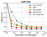
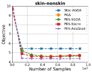
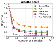
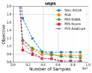
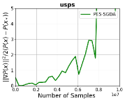
Figure 1: Results for Non-convex DRO.

Non-convex Distributionally Robust Optimization. This task has been considered in (Rafique et al., 2018). The problem is formulated as:

$$\begin{split}&\min\limits_{x\in\mathbb{R}^{d}}\max_{y\in\mathcal{S}}\sum_{i=1}^{n}y_{i}\phi(\log(1+\exp(-b_{i}\mathbf{a_{i}}^{T}x)))-\frac{\theta}{2}\|y-\frac{\mathbf{1}}{n}\|^{2}\end{split}$$ (11)

where $(\mathbf{a}_{i},b_{i})$ denotes feature label pair, $b_{i}\in\{-1,1\}$, $\phi(s)=\log(1+s/2)$ is a non-convex truncation function used to tackle outliers and noisy data, and $\mathcal{S}$ is a simplex. In experiments the simplex constraint is handled by a projection algorithm in Duchi et al. (2008). We conduct experiments on four datasets from LibSVM website (Chang and Lin, 2011), i.e., gisette-scale, cod-rna, skin-nonskin and usps. For skin-nonskin, we randomly partition the dataset into training set and testing set of equal size. For other data sets we use the provided training/testing split. For usps, we make the first class to be the positive class and merge the other 9 classes into the negative class.

We first verify the PL condition of primal problem $P(x)$ of (11) empirically. We plot $\|\nabla P(x)\|^{2}/2(P(x)-P(x_{*}))$ in the second figure of the Figure 1.

We compare three variants of our method (PES-SGDA, PES-STORM, PES-AdaGrad) with two baselines Stoc-AGDA (Yang et al., 2020a), PGA (algorithm 1 (Rafique et al., 2018)). For all algorithms, we set $\theta=10$. For Stoc-AGDA, the step sizes for $x$ and $y$ are set to be $\frac{\tau_{1}}{\lambda+t}$ and $\frac{\tau_{1}}{\lambda+t}$, respectively. $\tau_{1}$ and $\tau_{2}$ are tuned in $[1\sim 1e3]$. $\gamma$ is tuned in $[1\sim 1e4]$. For PES-SGDA, PES-STORM, and PES-AdaGrad, we set $T_{k}=T_{0}2^{k}$ and $\eta_{k}=\eta_{0}/2^{k}$, where $T_{0}$ and $\eta_{0}$ are tuned in $[500\sim 5000]$, $[0.1,0.05,0.01,0.001]$. $\gamma$ is tuned in $[1\sim 2000]$. The results are plotted in Figure 1. We can see that the proposed algorithms PES-SGDA, PES-STORM and PES-AdaGrad converge faster than the baselines in most cases. PES-STORM and PES-AdaGrad perform better than PES-SGDA on this task, which shows the potential to improve the performance by using STORM type variance techniques or adaptive methods when a task satisfies corresponding assumptions.

Deep AUC maximization. This task is similar to that considered in (Liu et al., 2020b). Deep AUC maximization with a square surrogate loss function is formulated as a NCSC min-max problem which has been introduced in the Section 4. We compare our algorithms, PES-SGDA (Option I), PES-OGDA (Option II), PES-AdaGrad (Option III), with five baseline methods, including stochastic gradient method (SGD) for solving a standard minimization formulation with cross-entropy loss, Stoc-AGDA (Yang et al., 2020a), PGA (algorithm 1 (Rafique et al., 2018)), PPD-SG and PPD-AdaGrad (Liu et al., 2020b) for solving the same AUC maximization problem. We learn ResNet-20 (He et al., 2016) with an ELU activation function.

For the parameter settings, we use a common stage-wise stepsize for SGD, i.e., the initial stepsize is divided by 10 at 40K, 60K of stochastic first-order oracle calls. For PPD-SG and PPD-AdaGrad, we follow the instructions in their works, i.e., $T_{k}=T_{0}3^{k},\eta_{k}=\eta_{0}/3^{k}$ and $T_{0},\eta_{0}$ and $\gamma$ are tuned in $[500\sim 2000]$, $[0.1,0.05,0.01,0.001]$, and $[100\sim 2000]$, respectively. For Stoc-AGDA, the stepsize strategy follows $\frac{\tau_{1}}{\lambda+t}$, $\frac{\tau_{2}}{\lambda+t}$ for the dual and primal variables, respectively, where $\tau_{1}\ll\tau_{2}$. The initial values $\tau_{1},\tau_{2}$, $\lambda$ are tuned in $[1,5,10,15]$, $[5,10,15,20]$, and $[1e3,1e4]$, respectively. For our methods, we adopt the same strategy as PPD-SG and PPD-AdaGrad to tune the parameters.

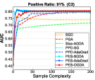
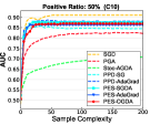
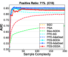
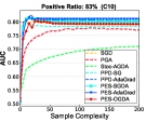
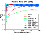
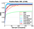
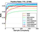
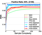
We compare on three benchmark datasets: Cat&Dog (C2) (Elson et al., 2007), CIFAR10 (C10), CIFAR100 (C100) (Krizhevsky et al., 2009) which have 2, 10, 100 classes, respectively. To fit our task, we convert them into imbalanced datasets following the instructions in (Liu et al., 2020b). We firstly construct the binary dataset by splitting the original dataset into two portions with equal size (50% positive: 50% negative) and then we randomly remove $90\%,80\%,60\%$ data from negative samples on training data, which generate the imbalanced datasets with a positive:negative ratio of 91/9, 83/17, 71/29, respectively. We keep the testing data unchanged. We set the batch size to 128 for all datasets.

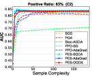
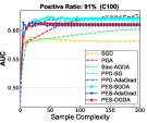
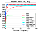
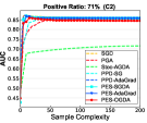
Figure 2: Comparison of testing AUC on Cat&Dog, CIFAR10, CIFAR100.

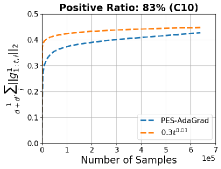
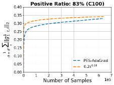
Figure 3: Verification of the Slow Growth Condition

The testing AUC curve of all algorithms are reported in Figure 2, where the sample complexity indicates the number of samples used in the training up to 80K of stochastic first-order oracle calls. From the results, we can see that SGD works better (or similar to) than AUC-based methods on the balanced data (50%). However, PES-SGDA and PES-AdaGrad generally outperform SGD when the data is imbalanced, and outperforms PGA and Stoc-AGDA in almost all cases. In addition, the proposed methods performs similarly sometimes better than PPD-SG/PPD-AdaGrad except on C100 (91% positive ratio). This is not surprising since PPD-SG/PPD-AdaGrad are designed for AUC maximization under the same PL condition by leveraging its structure and extra data samples for computing a restarted dual solution. In contrast, our algorithms directly use averaged dual solution for restarting. When the positive ratio is $91\%$ on C100, we observe that PPD-AdaGrad performs better than our algorithms, showing that using the extra data samples may help in the extreme imbalanced cases. We also observe that the Stoc-AGDA performs worst in all cases with $O(\frac{1}{t})$ stepsize. For our methods, PES-SGDA and PES-AdaGrad perform generally better than PES-OGDA. In Figure 3, we verify the slow growth condition, i.e. $\|g^{k}_{1,T_{k},i}\|\leq\delta T_{k}^{\alpha}$ used in the analysis of AdaGrad based algorithms, by plotting the $\frac{1}{d+d^{\prime}}\sum\limits_{i}\|g^{1}_{1:t,i}\|_{2}$ versus the sample complexity. We can seen that the growth of the aggregate of stochastic gradients is slower than the order of $O(\sqrt{T})$.

8 Conclusion

In this paper, we have presented generic stochastic algorithms for solving non-convex and strongly concave min-max optimization problems. We established convergence for both the objective gap and the duality gap under PL conditions of the objective function for different stochastic updates. The experiments on deep and non-deep learning tasks have demonstrated the effectiveness of our methods.

Acknowledgments and Disclosure of Funding

The feedback provided by the anonymous reviewers is greatly valued. We also wish to acknowledge the support received from the NSF Career Award #1844403, NSF Program #2110545, and NSF-Amazon Joint Program #2147253 for this work.

Appendix A Convergence of Duality Gap by Stoc-AGDA Algorithm

To compare our algorithm with Stoc-AGDA in terms of convergence of duality gap, we derive Lemma 17 based on Theorem 3.3 of (Yang et al., 2020a). We first present an auxiliary lemma which is an extension of the Danskin’s theorem.

Lemma 16 (Corollary of Theorem 1 of (Bernhard and Rapaport, 1995))

In the
min-max problem, when $f(x,y)$ is strong concave in $y$ for any $x$ then the gradient of the function $P(x)=\max_{y\in\mathcal{Y}}$ is $\nabla P(x)=\nabla_{x}f(x,\hat{y}(x))$ where $\hat{y}(x)=\arg\max_{y\in\mathcal{Y}}f(x,y)$.

Then the convergence of duality gap by Stoc-AGDA algorithm is given in next lemma.

Lemma 17

Supposes Assumption 1, 2, 4 and 6 hold. Stoc-AGDA would reach a $\epsilon$-duality gap by a stochastic first-order oracle call complexity of $O\left(\frac{\ell^{7}}{\mu^{2}\mu_{x}\mu_{y}^{5}\epsilon}\right)$.

Proof  Yang et al. (2020a) defines the measure as following potential function,

$$\begin{split}P_{t}=E[P(x_{t})-P(x_{*})]+\frac{1}{10}E[P(x_{t})-f(x_{t},y_{t})].\end{split}$$ (12)

By Theorem 3.3 of (Yang et al., 2020a), in Stoc-AGDA, $P_{t}\leq\hat{\epsilon}$ after $O\left(\frac{\ell^{5}}{\mu^{2}\mu_{y}^{4}\hat{\epsilon}}\right)$ stochastic first-order oracle calls. It directly follows that the objective gap will be less than $\hat{\epsilon}$ after $O\left(\frac{\ell^{5}}{\mu^{2}\mu_{y}^{4}\hat{\epsilon}}\right)$ stochastic first-order oracle calls, i.e.,

$$\begin{split}P(x_{t})-P(x_{*})\leq P_{t}\leq\hat{\epsilon}.\end{split}$$ (13)

Besides, after $O\left(\frac{\ell^{5}}{\mu^{2}\mu_{y}^{4}\hat{\epsilon}}\right)$ stochastic first-order oracle calls, we also have

$$f(x_{t},\hat{y}(x_{t}))-f(x_{t},y_{t})=P(x_{t})-f(x_{t},y_{t})\leq 10\hat{\epsilon},$$ (14)

where the equality holds by the Lemma 16. By the $\mu_{y}$-strong concavity of $f(x,\cdot)$, we have

$$\begin{split}\|y_{t}-\hat{y}(x_{t})\|^{2}\leq\frac{f(x_{t},\hat{y}(x_{t}))-f(x_{t},y_{t})}{2\mu_{y}}\leq\frac{5\hat{\epsilon}}{\mu_{y}},\end{split}$$ (15)

and

$$\begin{split}&\|\hat{y}(x_{t})-y_{*}\|^{2}\leq\frac{f(x_{t},\hat{y}(x_{t}))-f(x_{t},y_{*})}{2\mu_{y}}\\ &\leq\frac{f(x_{t},\hat{y}(x_{t}))-f(x_{*},y_{*})+f(x_{*},y_{*})-f(x_{t},y_{*})}{2\mu_{y}}\\ &\leq\frac{f(x_{t},\hat{y}(x_{t}))-f(x_{*},y_{*})}{2\mu_{y}}=\frac{P(x_{t})-P(x_{*})}{2\mu_{y}}\leq\frac{\hat{\epsilon}}{2\mu_{y}}.\end{split}$$ (16)

Thus,

$$\begin{split}\|y_{t}-y_{*}\|^{2}\overset{(a)}{\leq}2\|y_{t}-\hat{y}(x_{t})\|^{2}+2\|\hat{y}(x_{t})-y_{*}\|^{2}\leq\frac{11\hat{\epsilon}}{\mu_{y}},\end{split}$$ (17)

where $(a)$ holds since $\|\mathbf{a}-\mathbf{b}\|^{2}=\|\mathbf{a}-\mathbf{c}+\mathbf{c}-\mathbf{b}\|^{2}\leq 2\|\mathbf{a}-\mathbf{c}\|^{2}+2\|\mathbf{c}-\mathbf{b}\|^{2}$. Since $f(\cdot,\cdot)$ is $\ell$-smooth and $f(\cdot,y)$ satisfies $\mu_{x}$-PL condition for any $y$, we know $D(y)=\min\limits_{x^{\prime}}f(x^{\prime},y)$ is smooth with coefficient $\ell+\frac{\ell^{2}}{\mu_{x}}\leq\frac{2\ell^{2}}{\mu_{x}}$ (Nouiehed et al., 2019; Yang et al., 2020a). Thus,

$$\begin{split}f(x_{*},y_{*})-f(\hat{x}(y_{t}),y_{t})=D(y_{*})-D(y_{t})\leq\frac{2\ell^{2}}{2\mu_{x}}\|y_{t}-y_{*}\|^{2}\leq\frac{11\ell^{2}\hat{\epsilon}}{\mu_{x}\mu_{y}},\end{split}$$ (18)

where the first equality holds by Lemma A.5 of (Nouiehed et al., 2019).

Then we know the duality gap is

$$\begin{split}f(x_{t},\hat{y}(x_{t}))-f(\hat{x}(y_{t}),y_{t})&=f(x_{t},\hat{y}(x_{t}))-f(x_{*},y_{*})+f(x_{*},y_{*})-f(\hat{x}(y_{t}),y_{t})\\ &\leq\hat{\epsilon}+\frac{11\ell^{2}\hat{\epsilon}}{\mu_{x}\mu_{y}}.\end{split}$$ (19)

To make the duality gap less than $\epsilon$, we need $\hat{\epsilon}\leq O\left(\frac{\mu_{x}\mu_{y}\epsilon}{\ell^{2}}\right)$. Therefore, it takes $O\left(\frac{\ell^{7}}{\mu^{2}\mu_{x}\mu_{y}^{5}\epsilon}\right)$ stochastic first-order oracle calls to have a $\epsilon$-duality gap for the Algorithm Stoc-AGDA that has been proposed in (Yang et al., 2020a).  

Appendix B Convergence Analysis of PES-SGDA

We present the convergence rate of primal gap and duality gap if SGDA update is used in Algorithm 2. Since the proof is similar to the version with Option II: OGDA as update, we include the proof in later sections together with the version using OGDA update.

Theorem 18

Consider Algorithm 1 that uses Option I: SGDA update in subroutine Algorithm 2. Suppose Assumption 1, 3, 4 hold. Assume $\mathbb{E}\|\nabla_{x}f(x,y;\xi)\|^{2}\leq B^{2}$ and
$\mathbb{E}\|\nabla_{y}f(x,y;\xi)\|^{2}\leq B^{2}$. Take $\gamma=2\rho$ and denote $\hat{L}=L+2\rho$ and $c=4\rho+\frac{248}{53}\hat{L}\in O(L+\rho)$. Define $\Delta_{k}=P(x_{0}^{k})-P(x_{*})+\frac{8\hat{L}}{53c}\emph{\text{Gap}}_{k}(x_{0}^{k},y_{0}^{k})$ and $\epsilon_{0}=\emph{\text{Gap}}(\bar{x}_{0},\bar{y}_{0})$. Then we can set $\eta_{k}=\eta_{0}\exp(-(k-1)\frac{2\mu}{c+2\mu})\leq\frac{1}{\rho}$, $T_{k}=\left\lceil\frac{212C_{1}}{\eta_{0}\min\{\rho,\mu_{y}\}}\exp\left((k-1)\frac{2\mu}{c+2\mu}\right)\right\rceil$. After $K=\left\lceil\max\left\{\frac{c+2\mu}{2\mu}\log\frac{4\epsilon_{0}}{\epsilon},\frac{c+2\mu}{2\mu}\log\frac{80\eta_{0}\hat{L}KB_{2}}{(c+2\mu)\epsilon}\right\}\right\rceil$ stages, we can have $\Delta_{K+1}\leq\epsilon$. The total stochastic first-order oracle call complexity is $\widetilde{O}\left(\frac{(L+\rho)^{2}B^{2}}{\mu^{2}\min\{\rho,\mu_{y}\}\epsilon}\right)$.

Remark. The bounded stochastic gradient assumption i.e., $\mathbb{E}[\|\nabla_{x}f(x,y;\xi)\|^{2}]\leq B^{2}$ and $\mathbb{E}[\|\nabla_{y}f(x,y;\xi)\|^{2}]\leq B^{2}$ is only used for the analysis of our algorithm employing the SGDA update (Option I), and it is not used for other updates. It is notable that in min-max optimization it is an open question to get rid of the bounded stochastic gradient assumption for the vanilla SGDA updates in order to establish convergence bound for the duality gap. To the best of our knowledge, in the existing works over the gap convergence of stochastic min-max optimization that can achieve state-of-the-art complexity, they either use this bounded stochastic gradient assumption Nemirovski et al. (2009); Yan et al. (2020), or use some extra steps other than simple SGDA (Juditsky et al., 2011; Zhao, 2022; Hsieh et al., 2019; Zhao et al., 2019; Yang et al., 2020a).

Corollary 19

Under the same setting as in Theorem 18 and suppose Assumption 6 holds aw well. To reach an $\epsilon$-duality gap, it takes a total stochastic first-order oracle call complexity of $\widetilde{O}\left(\frac{(L+\rho)^{2}(\rho/\mu_{x}+1)B^{2}}{\mu^{2}\min\{\rho,\mu_{y}\}\epsilon}\right)$.

Theorem 20

Suppose Assumption 1, 6, 3 hold and $0<\rho\leq\frac{\mu}{8}$. Assume $\mathbb{E}\|\nabla_{x}f(x,y;\xi)\|^{2}\leq B^{2}$ and $\mathbb{E}\|\nabla_{y}f(x,y;\xi)\|^{2}\leq B^{2}$. Take $\gamma=2\rho$. Define $\Delta_{k}=475(P(x_{0}^{k})-P(x_{*}))+57\emph{\text{Gap}}_{k}(x_{0}^{k},y_{0}^{k})$ and $\epsilon_{0}=\emph{\text{Gap}}(\bar{x}_{0},\bar{y}_{0})$. Then we can set $\eta_{k}=\eta_{0}\exp(-\frac{k-1}{16})\leq\frac{1}{\rho}$, $T_{k}=\left\lceil\frac{768}{\eta_{0}\min\{\mu/8,\mu_{y}\}}\exp\left(\frac{k-1}{16}\right)\right\rceil$. After $K=\left\lceil\max\left\{16\log\frac{1200\epsilon_{0}}{\epsilon},16\log\frac{6000\eta_{0}KB^{2}}{\epsilon}\right\}\right\rceil$ stages, we can have $\Delta_{K+1}\leq\epsilon$. The total stochastic first-order oracle call complexity is $\widetilde{O}\left(\frac{B^{2}}{\min\{\mu,\mu_{y}\}\epsilon}\right)$.

Corollary 21

Under the same setting as in Theorem 20 and suppose Assumption 6 holds as well. To reach an $\epsilon$-duality gap, it takes total stochastic first-order oracle call complexity of $\widetilde{O}\left(\frac{(\mu/\mu_{x}+1)B^{2}}{\min\{\mu,\mu_{y}\}\epsilon}\right)$.

Appendix C One Stage Analysis of PES-OGDA

We need the following lemmas from (Nemirovski, 2004).

Lemma 22 (Lemma 3.1 of (Nemirovski, 2004))

For $z_{0}\in\mathcal{Z}$, let $w_{1}=\Pi_{z_{0}}(\zeta_{1})$, $w_{2}=\Pi_{z_{0}}(\zeta_{2})$. For any $z\in\mathcal{Z}$,

$$\begin{split}\langle\zeta_{2},w_{1}-z\rangle\leq\frac{1}{2}\|z-z_{0}\|^{2}-\frac{1}{2}\|w_{2}-z\|^{2}-\frac{1}{2}\|w_{1}-z_{0}\|^{2}-\frac{1}{2}\|w_{1}-w_{2}\|^{2}+\|\zeta_{1}-\zeta_{2}\|^{2}.\hfill\end{split}$$ (20)

Lemma 23 (Corollary 2 of (Juditsky et al., 2011))

Let $\zeta_{1},\zeta_{2},...$ be a sequence, we define a corresponding sequence $\{v_{t}\in\mathcal{Z}\}_{t=0}^{T}$ as

$$\begin{split}v_{t}=\Pi_{v_{t-1}}(\zeta_{t}),v_{0}\in\mathcal{Z},\end{split}$$ (21)

we have for any $u\in\mathcal{Z}$,

$$\begin{split}\sum\limits_{t=1}^{T}\left\langle\zeta_{t},v_{t-1}-u\right\rangle\leq\frac{1}{2}\|v_{0}-u\|^{2}+\frac{1}{2}\sum\limits_{t=1}^{T}\|\zeta_{t}\|^{2}.\end{split}$$ (22)

Next we present the lemma that guarantees the converge of one call of Algorithm 2 with Option II: OGDA update.

Lemma 24

Suppose $f(x,y)$ is convex-concave and Assumption 2 holds. By running Algorithm 2 with OGDA update and input $(f,x_{0},y_{0},\eta\leq\frac{1}{4\sqrt{3}\ell},T)$, we have

$$\begin{split}\mathbb{E}[f(\bar{x},\hat{y}(\bar{x}))-f(\hat{x}(\bar{y}),\bar{y})]&{\leq}\frac{1}{\eta T}\mathbb{E}(\|\hat{x}(\bar{y})-x_{0}\|^{2}+\|\hat{y}(\bar{x})-y_{0}\|^{2})+13\eta\sigma^{2}.\end{split}$$ (23)

Proof [Proof of Lemma 24] Applying Lemma 22 with $z_{0}=\tilde{z}_{t-1}$, $\zeta_{1}=\eta\mathcal{G}(z_{t-1};\xi_{t-1})$, $\zeta_{2}=\eta\mathcal{G}(z_{t};\xi_{t})$, and accordingly $w_{1}=z_{t}$, $w_{2}=\tilde{z}_{t}$, we get for any $z\in\mathcal{Z}$,

$$\begin{split}\langle\mathcal{G}(z_{t};\xi_{t}),z_{t}-z\rangle\leq&\frac{1}{2\eta}[\|z-\tilde{z}_{t-1}\|^{2}-\|\tilde{z}_{t}-z\|^{2}]-\frac{1}{2\eta}[\|z_{t}-\tilde{z}_{t-1}\|^{2}+\|z_{t}-\tilde{z}_{t}\|^{2}]\\ &+\eta\|\mathcal{G}(z_{t-1};\xi_{t-1})-\mathcal{G}(z_{t};\xi_{t})\|^{2}.\end{split}$$ (24)

Taking average over $t=1,...,T$ and by the convexity of $f(x,y)$ in $x$, we have for any $x\in\mathcal{X}$,

$$\begin{split}&\frac{1}{T}\sum\limits_{t=1}^{T}\langle\mathcal{G}(z_{t};\xi_{t}),z_{t}-z\rangle\leq\frac{\|z-\tilde{z}_{0}\|^{2}}{2\eta T}-\frac{1}{2\eta T}\sum\limits_{t=1}^{T}(\|z_{t}-\tilde{z}_{t-1}\|^{2}+\|z_{t}-\tilde{z}_{t}\|^{2})\\ &~{}~{}~{}~{}~{}~{}~{}~{}~{}~{}~{}~{}~{}~{}~{}~{}~{}~{}~{}~{}~{}~{}~{}~{}~{}~{}~{}~{}~{}~{}~{}~{}+\frac{\eta}{T}\sum\limits_{t=1}^{T}\|\mathcal{G}(z_{t-1};\xi_{t-1})-\mathcal{G}(z_{t};\xi_{t})\|^{2}\\ &\leq\frac{\|z-z_{0}\|^{2}}{2\eta T}-\frac{1}{2\eta T}\sum\limits_{t=1}^{T}(\|z_{t}-\tilde{z}_{t-1}\|^{2}+\|z_{t}-\tilde{z}_{t}\|^{2})+\frac{3\eta}{T}\sum\limits_{t=1}^{T}\|F(z_{t-1})-F(z_{t})\|^{2}\\ &~{}~{}~{}~{}~{}+\frac{3\eta}{T}\sum\limits_{t=1}^{T}(\|\mathcal{G}(z_{t};\xi_{t})-F(z_{t})\|^{2}+\|\mathcal{G}(z_{t-1};\xi_{t-1})-F(z_{t-1})\|^{2}),\end{split}$$ (25)

where the last inequality is due to $\left\|\sum\limits_{k=1}^{K}\mathbf{a}_{k}\right\|^{2}\leq K\sum\limits_{k=1}^{K}\left\|\mathbf{a}_{k}\right\|^{2}$. Note that

$$\begin{split}&\sum\limits_{t=1}^{T}(\|z_{t}-\tilde{z}_{t-1}\|^{2}+\|z_{t}-\tilde{z}_{t}\|^{2})=\sum\limits_{t=0}^{T-1}\|z_{t+1}-\tilde{z}_{t}\|^{2}+\sum\limits_{t=1}^{T}\|z_{t}-\tilde{z}_{t}\|^{2}\\ &=\sum\limits_{t=1}^{T-1}\|z_{t+1}-\tilde{z}_{t}\|^{2}+\|z_{1}-\tilde{z}_{0}\|^{2}+\sum\limits_{t=1}^{T-1}\|z_{t}-\tilde{z}_{t}\|^{2}\geq\frac{1}{2}\sum\limits_{t=1}^{T-1}\|z_{t}-z_{t+1}\|^{2}+\|z_{1}-\tilde{z}_{0}\|^{2}\\ &\geq\frac{1}{2}\sum\limits_{t=0}^{T-1}\|z_{t}-z_{t+1}\|^{2}=\frac{1}{2}\sum\limits_{t=1}^{T}\|z_{t-1}-z_{t}\|^{2}.\end{split}$$ (26)

By the $\ell$-smoothness of $f(x,y)$, we have

$$\begin{split}\|F(z_{t-1})-F(z_{t})\|^{2}=&\|\nabla_{x}f(x_{t},y_{t})-\nabla_{x}f(x_{t-1},y_{t-1})\|^{2}+\|\nabla_{y}f(x_{t},y_{t})-\nabla_{y}f(x_{t-1},y_{t-1})\|^{2}\\ \leq&2\|\nabla_{x}f(x_{t},y_{t})-\nabla_{x}f(x_{t},y_{t-1})\|^{2}+2\|\nabla_{x}f(x_{t},y_{t-1})-\nabla_{x}f(x_{t-1},y_{t-1})\|^{2}\\ &+2\|\nabla_{y}f(x_{t},y_{t})-\nabla_{y}f(x_{t},y_{t-1})\|^{2}+2\|\nabla_{y}f(x_{t},y_{t-1})-\nabla_{y}f(x_{t-1},y_{t-1})\|^{2}\\ \leq&2\ell^{2}\|y_{t}-y_{t-1}\|^{2}+2\ell^{2}\|x_{t}-x_{t-1}\|^{2}+2\ell^{2}\|y_{t}-y_{t-1}\|^{2}+2\ell^{2}\|x_{t}-x_{t-1}\|^{2}\\ =&4\ell^{2}\|z_{t-1}-z_{t}\|^{2}.\end{split}$$

Denote $\Theta_{t}=F(z_{t})-\mathcal{G}(z_{t};\xi_{t})$. With the above two inequalities, (25) becomes

$$\begin{split}&\frac{1}{T}\sum\limits_{t=1}^{T}\langle\mathcal{G}(z_{t};\xi_{t}),z_{t}-z\rangle\\ &\leq\frac{\|z-z_{0}\|^{2}}{2\eta T}-\frac{1}{4\eta T}\sum\limits_{t=1}^{T}\|z_{t-1}-z_{t}\|^{2}+\frac{12\eta\ell^{2}}{T}\sum\limits_{t=1}^{T}\|z_{t-1}-z_{t}\|^{2}+\frac{3\eta}{T}\sum\limits_{t=1}^{T}(\|\Theta_{t}\|^{2}+\|\Theta_{t-1}\|^{2})\\ &\leq\frac{\|z-z_{0}\|^{2}}{2\eta T}+\frac{3\eta}{T}\sum\limits_{t=1}^{T}(\|\Theta_{t}\|^{2}+\|\Theta_{t-1}\|^{2}),\end{split}$$ (27)

where the last inequality holds because $\eta\leq\frac{1}{4\sqrt{3}\ell}$.

Define a virtual sequence $\{\hat{z}_{t}\in\mathcal{X}\}_{t=0}^{T}$ as

$$\begin{split}\hat{z}_{t}=\Pi_{\hat{z}_{t-1}}(\eta\Theta_{t}),\hat{z}_{0}=z_{0}.\end{split}$$ (28)

Applying Lemma 23 with $\zeta_{t}=\eta\Theta_{t}=\eta(F(z_{t})-\mathcal{G}(z_{t};\xi_{t})),v_{t}=\hat{z}_{t}$ and $u=z$, we have for any $z\in\mathcal{Z}$,

$$\begin{split}\frac{1}{T}\sum\limits_{t=1}^{T}\langle\Theta_{t},\hat{z}_{t-1}-z\rangle\leq\frac{1}{2\eta T}\|z_{0}-z\|^{2}+\frac{\eta}{2T}\sum\limits_{t=1}^{T}\|\Theta_{t}\|^{2}.\end{split}$$ (29)

Using (27) and (29), we get

$$\begin{split}&\frac{1}{T}\sum\limits_{t=1}^{T}\langle F(z_{t}),z_{t}-z\rangle=\frac{1}{T}\sum\limits_{t=1}^{T}[\langle\mathcal{G}(z_{t};\xi_{t}),z_{t}-z\rangle\!+\langle\Theta_{t},z_{t}-z\rangle]\\ &=\frac{1}{T}\sum\limits_{t=1}^{T}\langle\mathcal{G}(z_{t};\xi_{t}),z_{t}-z\rangle\!+\frac{1}{T}\sum\limits_{t=1}^{T}\langle\Theta_{t},z_{t}\!-\!\hat{z}_{t-1}\rangle+\!\frac{1}{T}\sum\limits_{t=1}^{T}\langle\Theta_{t},\hat{z}_{t-1}\!-z\rangle\\ &\leq\frac{1}{\eta T}\|z_{0}-z\|^{2}+\frac{\eta}{T}\sum\limits_{t=1}^{T}\left(\frac{7}{2}\|\Theta_{x,t}\|^{2}+3\|\Theta_{x,t-1}\|^{2}\right)+\!\frac{1}{T}\sum\limits_{t=1}^{T}\langle\Theta_{x,t},x_{t}\!-\!\hat{x}_{t-1}\rangle.\end{split}$$ (30)

Note

$$\mathbb{E}[\langle\Theta_{t},z_{t}-\hat{z}_{t-1}\rangle|z_{t},\hat{z}_{t-1},\Theta_{t-1},...,\Theta_{0}]=0,$$

and by Assumption 2

$$\mathbb{E}[\|\Theta_{t}\|^{2}|z_{t},\tilde{z}_{t-1},\Theta_{t-1},...,\Theta_{0}]\leq 2\sigma^{2}.$$

Thus, taking expectation on both sides of (30), we get

$$\begin{split}\mathbb{E}\left[\frac{1}{T}\sum\limits_{t=1}^{T}\langle F(z_{t}),z_{t}-z\rangle\right]\leq&\frac{1}{\eta T}\mathbb{E}\left[\|z_{0}-z\|^{2}\right]+13\eta\sigma^{2}.\end{split}$$ (31)

By the fact $f(x,y)$ is convex-concave,

$$\begin{split}\mathbb{E}[f(\bar{x},y)-f(x,\bar{y})]\leq&\mathbb{E}\left[\frac{1}{T}\sum\limits_{t=1}^{T}(f(x_{t},y)-f(x,y_{t}))\right]\\ =&\mathbb{E}\left[\frac{1}{T}\sum\limits_{t=1}^{T}(f(x_{t},y)-f(x_{t},y_{t})+f(x_{t},y_{t})-f(x,y_{t}))\right]\\ \leq&\mathbb{E}\left[\frac{1}{T}\sum\limits_{t=1}^{T}(\langle-\nabla_{y}f(x_{t},y_{t}),y_{t}\!-\!y\rangle+\langle\nabla_{x}f(x_{t},y_{t}),x_{t}\!-\!x\rangle)\right]\\ =&\mathbb{E}\left[\frac{1}{T}\sum\limits_{t=1}^{T}\langle F(z_{t}),z_{t}-z\rangle\right]\leq\frac{1}{\eta T}E[\|z_{0}-z\|^{2}]+13\eta\sigma^{2}.\end{split}$$ (32)

Then we can conclude by plugging in $z=(x,y)=(\hat{x}(\bar{y}),\hat{y}(\bar{x}))$.  

Appendix D Proof of Theorem 10 and Theorem 18

Before we prove these two theorems, we first present two lemmas from (Yan et al., 2020) and we introduce Theorem 27 that unifies the proof of Theorem 10 and Theorem 18.

Lemma 25 (Lemma 1 of (Yan et al., 2020))

Suppose a function $h(x,y)$ is $\lambda_{1}$-strongly convex in $x$ and $\lambda_{2}$-strongly concave in $y$. Consider the following problem

$$\min\limits_{x\in\mathcal{X}}\max\limits_{y\in\mathcal{Y}}h(x,y),$$

where $\mathcal{X}$ and $\mathcal{Y}$ are convex sets. Denote $\hat{x}_{h}(y)=\arg\min\limits_{x^{\prime}\in\mathcal{X}}h(x^{\prime},y)$ and $\hat{y}_{h}(x)=\arg\max\limits_{y^{\prime}\in\mathcal{Y}}h(x,y^{\prime})$. Suppose we have two solutions $(x_{0},y_{0})$ and $(x_{1},y_{1})$. Then the following relation between variable distance and duality gap holds

$$\begin{split}\frac{\lambda_{1}}{4}\|\hat{x}_{h}(y_{1})-x_{0}\|^{2}+\frac{\lambda_{2}}{4}\|\hat{y}_{h}(x_{1})-y_{0}\|^{2}\leq&\max\limits_{y^{\prime}\in\mathcal{Y}}h(x_{0},y^{\prime})-\min\limits_{x^{\prime}\in\mathcal{X}}h(x^{\prime},y_{0})\\ &+\max\limits_{y^{\prime}\in\mathcal{Y}}h(x_{1},y^{\prime})-\min\limits_{x^{\prime}\in\mathcal{X}}h(x^{\prime},y_{1}).\end{split}$$ (33)

Lemma 26 (Lemma 5 of (Yan et al., 2020))

We have the following lower bound for $\emph{\text{Gap}}_{k}(\bar{x}_{k},\bar{y}_{k})$

$$\emph{\text{Gap}}_{k}(\bar{x}_{k},\bar{y}_{k})\geq\frac{3}{50}\emph{\text{Gap}}_{k+1}(x_{0}^{k+1},y_{0}^{k+1})+\frac{4}{5}(P(x_{0}^{k+1})-P(x_{0}^{k})),$$

where $x_{0}^{k+1}=\bar{x}_{k}$ and $y_{0}^{k+1}=\bar{y}_{k}$.

We will introduce the following theorem that can unify the proof of Theorem 10 and Theorem 18 since their have pretty similar forms of bounds in solving the subproblem.

Theorem 27

Suppose Assumption 1 and Assumption 4 hold. Assume we have a subroutine in the $k$-th stage of Algorithm 1 that can return $\bar{x}_{k},\bar{y}_{k}$ such that

$$\begin{split}\mathbb{E}[\emph{\text{Gap}}_{k}(\bar{x}_{k},\bar{y}_{k})]\leq\frac{C_{1}}{\eta_{k}T_{k}}\mathbb{E}[\|\hat{x}_{k}(\bar{y}_{k})-x_{0}^{k}\|^{2}+\|\hat{y}_{k}(\bar{x}_{k})-y_{0}^{k}\|^{2}]+\eta_{k}C_{2},\end{split}$$ (34)

where $C_{1}$ and $C_{2}$ are constants corresponding to the specific subroutine. Take $\gamma=2\rho$ and denote $\hat{L}=L+2\rho$ and $c=4\rho+\frac{248}{53}\hat{L}\in O(L+\rho)$. Define $\Delta_{k}=P(x_{0}^{k})-P(x_{*})+\frac{8\hat{L}}{53c}\emph{\text{Gap}}_{k}(x_{0}^{k},y_{0}^{k})$ and $\epsilon_{0}=\emph{\text{Gap}}(\bar{x}_{0},\bar{y}_{0})$. Then we can set $\eta_{k}=\eta_{0}\exp(-(k-1)\frac{2\mu}{c+2\mu})$, $T_{k}=\left\lceil\frac{212C_{1}}{\eta_{0}\min\{\rho,\mu_{y}\}}\exp\left((k-1)\frac{2\mu}{c+2\mu}\right)\right\rceil$. After $K=\left\lceil\max\left\{\frac{c+2\mu}{2\mu}\log\frac{4\epsilon_{0}}{\epsilon},\frac{c+2\mu}{2\mu}\log\frac{16\eta_{0}\hat{L}KC_{2}}{(c+2\mu)\epsilon}\right\}\right\rceil$ stages, we can have $\Delta_{K+1}\leq\epsilon$. The total stochastic first-order oracle call complexity is $\widetilde{O}\left(\max\left\{\frac{(L+\rho)C_{1}\epsilon_{0}}{\eta_{0}\mu\min\{\rho,\mu_{y}\}\epsilon},\frac{(L+\rho)^{2}C_{2}}{\mu^{2}\min\{\rho,\mu_{y}\}\epsilon}\right\}\right)$.

Proof [Proof of Theorem 27] Since $f(x,y)$ is $\rho$-weakly convex in $x$ for any $y$, $P(x)=\max\limits_{y^{\prime}\in\mathcal{Y}}f(x,y^{\prime})$ is also $\rho$-weakly convex. Taking $\gamma=2\rho$, we have

$$\begin{split}P(\bar{x}_{k-1})&\geq P(\bar{x}_{k})+\langle\nabla P(\bar{x}_{k}),\bar{x}_{k-1}-\bar{x}_{k}\rangle-\frac{\rho}{2}\|\bar{x}_{k-1}-\bar{x}_{k}\|^{2}\\ &=P(\bar{x}_{k})+\langle\nabla P(\bar{x}_{k})+2\rho(\bar{x}_{k}-\bar{x}_{k-1}),\bar{x}_{k-1}-\bar{x}_{k}\rangle+\frac{3\rho}{2}\|\bar{x}_{k-1}-\bar{x}_{k}\|^{2}\\ &\overset{(a)}{=}P(\bar{x}_{k})+\langle\nabla P_{k}(\bar{x}_{k}),\bar{x}_{k-1}-\bar{x}_{k}\rangle+\frac{3\rho}{2}\|\bar{x}_{k-1}-\bar{x}_{k}\|^{2}\\ &\overset{(b)}{=}P(\bar{x}_{k})-\frac{1}{2\rho}\langle\nabla P_{k}(\bar{x}_{k}),\nabla P_{k}(\bar{x}_{k})-\nabla P(\bar{x}_{k})\rangle+\frac{3}{8\rho}\|\nabla P_{k}(\bar{x}_{k})-\nabla P(\bar{x}_{k})\|^{2}\\ &=P(\bar{x}_{k})-\frac{1}{8\rho}\|\nabla P_{k}(\bar{x}_{k})\|^{2}-\frac{1}{4\rho}\langle\nabla P_{k}(\bar{x}_{k}),\nabla P(\bar{x}_{k})\rangle+\frac{3}{8\rho}\|\nabla P(\bar{x}_{k})\|^{2},\end{split}$$ (35)

where $(a)$ and $(b)$ hold by the definition of $P_{k}(x)$.

Rearranging the terms in (35) yields

$$\begin{split}P(\bar{x}_{k})-P(\bar{x}_{k-1})&\leq\frac{1}{8\rho}\|\nabla P_{k}(\bar{x}_{k})\|^{2}+\frac{1}{4\rho}\langle\nabla P_{k}(\bar{x}_{k}),\nabla P(\bar{x}_{k})\rangle-\frac{3}{8\rho}\|\nabla P(\bar{x}_{k})\|^{2}\\ &\overset{(a)}{\leq}\frac{1}{8\rho}\|\nabla P_{k}(\bar{x}_{k})\|^{2}+\frac{1}{8\rho}(\|\nabla P_{k}(\bar{x}_{k})\|^{2}+\|\nabla P(\bar{x}_{k})\|^{2})-\frac{3}{8\rho}\|P(\bar{x}_{k})\|^{2}\\ &=\frac{1}{4\rho}\|\nabla P_{k}(\bar{x}_{k})\|^{2}-\frac{1}{4\rho}\|\nabla P(\bar{x}_{k})\|^{2}\\ &\overset{(b)}{\leq}\frac{1}{4\rho}\|\nabla P_{k}(\bar{x}_{k})\|^{2}-\frac{\mu}{2\rho}(P(\bar{x}_{k})-P(x_{*})),\end{split}$$ (36)

where $(a)$ holds by using $\langle\mathbf{a},\mathbf{b}\rangle\leq\frac{1}{2}(\|\mathbf{a}\|^{2}+\|\mathbf{b}\|^{2})$, and $(b)$ holds by the $\mu$-PL property of $P(x)$.

Thus, we have

$$\left(4\rho+2\mu\right)(P(\bar{x}_{k})-P(x_{*}))-4\rho(P(\bar{x}_{k-1})-P(x_{*}))\leq\|\nabla P_{k}(\bar{x}_{k})\|^{2}.$$ (37)

Since $\gamma=2\rho$, $f_{k}(x,y)$ is $\rho$-strongly convex in $x$ and $\mu_{y}$ strong concave in $y$. Apply Lemma 25 to $f_{k}$, we know that

$$\frac{\rho}{4}\|\hat{x}_{k}(\bar{y}_{k})-x_{0}^{k}\|^{2}+\frac{\mu_{y}}{4}\|\hat{y}_{k}(\bar{x}_{k})-y_{0}^{k}\|^{2}\leq{\text{Gap}}_{k}(x_{0}^{k},y_{0}^{k})+{\text{Gap}}_{k}(\bar{x}_{k},\bar{y}_{k}).$$ (38)

By the setting of $\eta_{k}=\eta_{0}\exp\left(-(k-1)\frac{2\mu}{c+2\mu}\right)$, and $T_{k}=\left\lceil\frac{212C_{1}}{\eta_{0}\min\{\rho,\mu_{y}\}}\exp\left((k-1)\frac{2\mu}{c+2\mu}\right)\right\rceil$, we note that $\frac{C_{1}}{\eta_{k}T_{k}}\leq\frac{\min\{\rho,\mu_{y}\}}{212}$. Applying (34), we have

$$\begin{split}&\mathbb{E}[{\text{Gap}}_{k}(\bar{x}_{k},\bar{y}_{k})]\leq\eta_{k}C_{2}+\frac{1}{53}\mathbb{E}\left[\frac{\rho}{4}\|\hat{x}_{k}(\bar{y}_{k})-x_{0}^{k}\|^{2}+\frac{\mu_{y}}{4}\|\hat{y}_{k}(\bar{x}_{k})-y_{0}^{k}\|^{2}\right]\\ &\leq\eta_{k}C_{2}+\frac{1}{53}\mathbb{E}\left[{\text{Gap}}_{k}(x_{0}^{k},y_{0}^{k})+{\text{Gap}}_{k}(\bar{x}_{k},\bar{y}_{k})\right].\end{split}$$ (39)

Since $P(x)$ is $L$-smooth and $\gamma=2\rho$, then $P_{k}(x)$ is $\hat{L}=(L+2\rho)$-smooth. According to Theorem 2.1.5 of (Nesterov, 2004), we have

$$\begin{split}&\mathbb{E}[\|\nabla P_{k}(\bar{x}_{k})\|^{2}]\leq 2\hat{L}\mathbb{E}(P_{k}(\bar{x}_{k})-\min\limits_{x\in\mathbb{R}^{d}}P_{k}(x))\leq 2\hat{L}\mathbb{E}[{\text{Gap}}_{k}(\bar{x}_{k},\bar{y}_{k})]\\ &=2\hat{L}\mathbb{E}[4{\text{Gap}}_{k}(\bar{x}_{k},\bar{y}_{k})-3{\text{Gap}}_{k}(\bar{x}_{k},\bar{y}_{k})]\\ &\leq 2\hat{L}\mathbb{E}\left[4\left(\eta_{k}C_{2}+\frac{1}{53}\left({\text{Gap}}_{k}(x_{0}^{k},y_{0}^{k})+{\text{Gap}}_{k}(\bar{x}_{k},\bar{y}_{k})\right)\right)-3{\text{Gap}}_{k}(\bar{x}_{k},\bar{y}_{k})\right]\\ &=2\hat{L}\mathbb{E}\left[4\eta_{k}C_{2}+\frac{4}{53}{\text{Gap}}_{k}(x_{0}^{k},y_{0}^{k})-\frac{155}{53}{\text{Gap}}_{k}(\bar{x}_{k},\bar{y}_{k})\right].\end{split}$$ (40)

Applying Lemma 26 to (40), we have

$$\begin{split}&\mathbb{E}[\|\nabla P_{k}(\bar{x}_{k})\|^{2}]\leq 2\hat{L}\mathbb{E}\bigg{[}4\eta_{k}C_{k}+\frac{4}{53}{\text{Gap}}_{k}(x_{0}^{k},y_{0}^{k})\\ &~{}~{}~{}~{}~{}~{}~{}~{}~{}~{}~{}~{}~{}~{}~{}~{}~{}~{}~{}~{}~{}~{}~{}~{}~{}~{}~{}~{}~{}~{}~{}~{}~{}~{}~{}~{}~{}~{}~{}~{}-\frac{155}{53}\left(\frac{3}{50}{\text{Gap}}_{k+1}(x_{0}^{k+1},y_{0}^{k+1})+\frac{4}{5}(P(x_{0}^{k+1})-P(x_{0}^{k}))\right)\bigg{]}\\ &=2\hat{L}\mathbb{E}\bigg{[}4\eta_{k}C_{2}\!+\!\frac{4}{53}{\text{Gap}}_{k}(x_{0}^{k},y_{0}^{k})\!-\!\frac{93}{530}{\text{Gap}}_{k+1}(x_{0}^{k+1},y_{0}^{k+1})\!-\!\frac{124}{53}(P(x_{0}^{k+1})-P(x_{0}^{k}))\bigg{]}.\end{split}$$

Combining this with (37), rearranging the terms, and defining a constant $c=4\rho+\frac{248}{53}\hat{L}\in O(L+\rho)$, we get

$$\begin{split}&\left(c+2\mu\right)\mathbb{E}[P(x_{0}^{k+1})-P(x_{*})]+\frac{93}{265}\hat{L}\mathbb{E}[{\text{Gap}}_{k+1}(x_{0}^{k+1},y_{0}^{k+1})]\\ &\leq\left(4\rho+\frac{248}{53}\hat{L}\right)\mathbb{E}[P(x_{0}^{k})-P(x_{*})]+\frac{8\hat{L}}{53}\mathbb{E}[{\text{Gap}}_{k}(x_{0}^{k},y_{0}^{k})]+8\eta_{k}\hat{L}C_{2}\\ &\leq c\mathbb{E}\left[P(x_{0}^{k})-P(x_{*})+\frac{8\hat{L}}{53c}{\text{Gap}}_{k}(x_{0}^{k},y_{0}^{k})\right]+8\eta_{k}\hat{L}C_{2}.\end{split}$$ (41)

Using the fact that $\hat{L}\geq\mu$,

$$\begin{split}(c+2\mu)\frac{8\hat{L}}{53c}=\left(4\rho+\frac{248}{53}\hat{L}+2\mu\right)\frac{8\hat{L}}{53(4\rho+\frac{248}{53}\hat{L})}\leq\frac{8\hat{L}}{53}+\frac{16\mu\hat{L}}{248\hat{L}}\leq\frac{93}{265}\hat{L}.\end{split}$$ (42)

Then, we have

$$\begin{split}&(c+2\mu)\mathbb{E}\left[P(x_{0}^{k+1})-P(x_{*})+\frac{8\hat{L}}{53c}{\text{Gap}}_{k+1}(x_{0}^{k+1},y_{0}^{k+1})\right]\\ &\leq c\mathbb{E}\left[P(x_{0}^{k})-P(x_{*})+\frac{8\hat{L}}{53c}{\text{Gap}}_{k}(x_{0}^{k},y_{0}^{k})\right]+8\eta_{k}\hat{L}C_{2}.\end{split}$$ (43)

Defining $\Delta_{k}=P(x_{0}^{k})-P(x_{*})+\frac{8\hat{L}}{53c}{\text{Gap}}_{k}(x_{0}^{k},y_{0}^{k})$, then

$$\begin{split}&\mathbb{E}[\Delta_{k+1}]\leq\frac{c}{c+2\mu}\mathbb{E}[\Delta_{k}]+\frac{8\eta_{k}\hat{L}C_{2}}{c+2\mu}.\end{split}$$ (44)

Using this inequality recursively, it yields

$$\begin{split}&E[\Delta_{K+1}]\leq\left(\frac{c}{c+2\mu}\right)^{K}E[\Delta_{1}]+\frac{8\hat{L}C_{2}}{c+2\mu}\sum\limits_{k=1}^{K}\left(\eta_{k}\left(\frac{c}{c+2\mu}\right)^{K+1-k}\right).\end{split}$$ (45)

By definition,

$$\begin{split}\Delta_{1}&=P(x_{0}^{1})-P(x_{*})+\frac{8\hat{L}}{53c}{\text{Gap}}_{1}(x_{0}^{1},y_{0}^{1})\\ &=P(\bar{x}_{0})-P(x_{*})+\left(f(\bar{x}_{0},\hat{y}_{1}(\bar{x}_{0}))+\frac{\gamma}{2}\|\bar{x}_{0}-\bar{x}_{0}\|^{2}-f(\hat{x}_{1}(\bar{y}_{0}),\bar{y}_{0})-\frac{\gamma}{2}\|\hat{x}_{1}(\bar{y}_{0})-\bar{x}_{0}\|^{2}\right)\\ &\leq\epsilon_{0}+f(\bar{x}_{0},\hat{y}_{1}(\bar{x}_{0}))-f(\hat{x}(\bar{y}_{0}),\bar{y}_{0})\leq 2\epsilon_{0}.\end{split}$$

Using inequality $1-x\leq\exp(-x)$, we have

$$\begin{split}&\mathbb{E}[\Delta_{K+1}]\leq\exp\left(\frac{-2\mu K}{c+2\mu}\right)\mathbb{E}[\Delta_{1}]+\frac{8\eta_{0}\hat{L}C_{2}}{c+2\mu}\sum\limits_{k=1}^{K}\exp\left(-\frac{2\mu K}{c+2\mu}\right)\\ &\leq 2\epsilon_{0}\exp\left(\frac{-2\mu K}{c+2\mu}\right)+\frac{8\eta_{0}\hat{L}C_{2}}{c+2\mu}K\exp\left(-\frac{2\mu K}{c+2\mu}\right).\end{split}$$

To make this less than $\epsilon$, it suffices to make

$$\begin{split}&2\epsilon_{0}\exp\left(\frac{-2\mu K}{c+2\mu}\right)\leq\frac{\epsilon}{2},\\ &\frac{8\eta_{0}\hat{L}C_{2}}{c+2\mu}K\exp\left(-\frac{2\mu K}{c+2\mu}\right)\leq\frac{\epsilon}{2}.\end{split}$$

Let $K$ be the smallest value such that $\exp\left(\frac{-2\mu K}{c+2\mu}\right)\leq\min\{\frac{\epsilon}{4\epsilon_{0}},\frac{(c+2\mu)\epsilon}{16\eta_{0}\hat{L}KC_{2}}\}$. We can set $K=\left\lceil\max\bigg{\{}\frac{c+2\mu}{2\mu}\log\frac{4\epsilon_{0}}{\epsilon},\frac{c+2\mu}{2\mu}\log\frac{16\eta_{0}\hat{L}KC_{2}}{(c+2\mu)\epsilon}\bigg{\}}\right\rceil$. Then, the total stochastic first-order oracle call complexity is

$$\sum\limits_{k=1}^{K}T_{k} \leq O\left(\frac{212C_{1}}{\eta_{0}\min\{\rho,\mu_{y}\}}\sum\limits_{k=1}^{K}\exp\left((k-1)\frac{2\mu}{c+2\mu}\right)\right)$$

$$\leq O\bigg{(}\frac{212C_{1}}{\eta_{0}\min\{\rho,\mu_{y}\}}\frac{\exp(K\frac{2\mu}{c+2\mu})-1}{\exp(\frac{2\mu}{c+2\mu})-1}\bigg{)}$$

$$\overset{(a)}{\leq}\widetilde{O}\left(\frac{cC_{1}}{\eta_{0}\mu\min\{\rho,\mu_{y}\}}\max\left\{\frac{\epsilon_{0}}{\epsilon},\frac{\eta_{0}\hat{L}KC_{2}}{(c+2\mu)\epsilon}\right\}\right)$$

$$\leq\widetilde{O}\left(\max\left\{\frac{(L+\rho)C_{1}\epsilon_{0}}{\eta_{0}\mu\min\{\rho,\mu_{y}\}\epsilon},\frac{(L+\rho)^{2}C_{2}}{\mu^{2}\min\{\rho,\mu_{y}\}\epsilon}\right\}\right),$$

where $(a)$ uses the setting of $K$ and $\exp(x)-1\geq x$, and $\widetilde{O}$ suppresses logarithmic factors.  

Proof [Proof of Theorem 10] With the above theorem, Theorem 10 directly follows. Noting Lemma 24, we can plug in $\eta_{0}=\frac{1}{2\sqrt{2}\ell}$, $C_{1}=1$ and $C_{2}=13\sigma^{2}$ to Theorem 27.  

Proof [Proof of Theorem 18] We need the following lemma to bound the convergence of the subproblem at each stage,

Lemma 28 (Lemma 4 of (Yan et al., 2020))

Suppose Assumption 1 holds,
$\mathbb{E}\|\nabla_{x}f(x_{t},y_{t};\xi_{t})\|^{2}\leq B^{2}$ and $\mathbb{E}\|\nabla_{y}f(x_{t},y_{t};\xi_{t})\|^{2}\leq B^{2}$. Set $\gamma=2\rho$. By running Algorithm 1 with Option II: SGDA, it holds for $k\geq 1$,

$$\begin{split}E[\emph{\text{Gap}}_{k}(\bar{x}_{k},\bar{y}_{k})]\leq 5\eta_{k}B^{2}+\frac{1}{T_{k}}\bigg{\{}\left(\frac{1}{\eta_{k}}+\frac{\rho}{2}\right)E[\|\hat{x}_{k}(\bar{y}_{k})-x_{0}^{k}\|^{2}]+\frac{1}{\eta_{k}}E[\|\hat{y}_{k}(\bar{x}_{k})-y_{0}^{k}\|^{2}]\bigg{\}}.\end{split}$$

Using this lemma , we can set $\gamma=2\rho$ and $\eta_{0}=\frac{1}{\rho}$. Then it follows that

$$\begin{split}E[\text{Gap}_{k}(\bar{x}_{k},\bar{y}_{k})]\leq 5\eta_{k}B^{2}+\frac{2}{\eta_{k}T_{k}}\left(E[\|\hat{x}_{k}(\bar{y}_{k})-x_{0}^{k}\|^{2}]+E[\|\hat{y}_{k}(\bar{x}_{k})-y_{0}^{k}\|^{2}\right).\end{split}$$

We plug in $\eta_{0}\leq\frac{1}{\rho}$, $C_{1}=2$ and $C_{2}=5B^{2}$ to Theorem 27 and the conclusion follows.  

Appendix E Proof of Theorem 11 and Theorem 20

We first present a lemma by plugging in Lemma 8 of (Yan et al., 2020). And then we a theorem that can unify the proof of Theorem 11 and Theorem 20. In the last, we prove Theorem 11 and Theorem 20.

Lemma 29 (Lemma 8 of (Yan et al., 2020))

Suppose $f(x,y)$ is $\frac{\mu}{8}$-weakly convex in $x$ for any $y$ and set $\gamma=\frac{\mu}{4}$. Thus, $f_{k}(x,y)$ is $\frac{\mu}{8}$-strongly convex in $x$. Then $\emph{\text{Gap}}_{k}(\bar{x}_{k},\bar{y}_{k})$ can be lower bounded by the following inequalities

$$\emph{\text{Gap}}_{k}(\bar{x}_{k},\bar{y}_{k})\geq\left(3-\frac{2}{\alpha}\right)\emph{\text{Gap}}_{k+1}(x_{0}^{k+1},y_{0}^{k+1})-\frac{\mu\alpha}{8(1-\alpha)}\|x_{0}^{k+1}-x_{0}^{k}\|^{2},(0<\alpha\leq 1),$$ (46)

and

$$\emph{\text{Gap}}_{k}(\bar{x}_{k},\bar{y}_{k})\geq P(x_{0}^{k+1})-P(x_{0}^{k})+\frac{\mu}{8}\|\bar{x}_{k}-x_{0}^{k}\|^{2},where~{}P(x)=\max\limits_{y^{\prime}\in\mathcal{Y}}f(x,y^{\prime}).$$ (47)

Theorem 30

Suppose $0<\rho\leq\frac{\mu}{8}$ and suppose Assumption 1, 2, 3, 4 hold. Assume we have a subroutine in the $k$-th stage of Algorithm 1 that can return $\bar{x}_{k},\bar{y}_{k}$ such that

$$\begin{split}\mathbb{E}[\emph{\text{Gap}}_{k}(\bar{x}_{k},\bar{y}_{k})]\leq\frac{C_{1}}{\eta_{k}T_{k}}\mathbb{E}[\|x-x_{0}^{k}\|^{2}+\|y-y_{0}^{k}\|^{2}]+\eta_{k}C_{2},\end{split}$$ (48)

where $C_{1}$ and $C_{2}$ are constants corresponding to the specific subroutine. Take $\gamma=\frac{\mu}{4}$. Define $\Delta_{k}=475(P(x_{0}^{k})-P(x_{*}))+57\emph{\text{Gap}}_{k}(x_{0}^{k},y_{0}^{k})$ and $\epsilon_{0}=\emph{\text{Gap}}(\bar{x}_{0},\bar{y}_{0})$. Then we can set $\eta_{k}=\eta_{0}\exp(-\frac{k-1}{16})\leq\frac{1}{2\sqrt{2}\ell}$, $T_{k}=\left\lceil\frac{384C_{1}}{\eta_{0}\min\{\mu/8,\mu_{y}\}}\exp\left(\frac{k-1}{16}\right)\right\rceil$. After
$K=\left\lceil\max\left\{16\log\frac{1200\epsilon_{0}}{\epsilon},16\log\frac{1200\eta_{0}KC_{2}}{\epsilon}\right\}\right\rceil$ stages, we can have $\Delta_{K+1}\leq\epsilon$. The total stochastic first-order oracle call complexity is $\widetilde{O}\left(\max\left\{\frac{C_{1}\epsilon_{0}}{\eta_{0}\min\{\mu,\mu_{y}\}\epsilon},\frac{C_{2}}{\min\{\mu,\mu_{y}\}\epsilon}\right\}\right)$.

Proof [Proof of Theorem 30] We have the following relation between $P(x_{0}^{k})-P(x_{*})$ and ${\text{Gap}}_{k}(x_{0}^{k},y_{0}^{k})$,

$$\begin{split}&P(x_{0}^{k})-P(x_{*})=f(x_{0}^{k},\hat{y}(x_{0}^{k}))-f(x_{*},y_{*})\leq f(x_{0}^{k},\hat{y}(x_{0}^{k}))-f(x_{*},y_{0}^{k})\\ &=f(x_{0}^{k},\hat{y}(x_{0}^{k}))+\frac{\gamma}{2}\|x_{0}^{k}-x_{0}^{k}\|^{2}-f(x_{*},y_{0}^{k})-\frac{\gamma}{2}\|x_{*}-x_{0}^{k}\|^{2}+\frac{\gamma}{2}\|x_{*}-x_{0}^{k}\|^{2}\\ &=f_{k}(x_{0}^{k},\hat{y}(x_{0}^{k}))-f_{k}(x_{*},y_{0}^{k})+\frac{\gamma}{2}\|x_{*}-x_{0}^{k}\|^{2}\\ &\leq\hat{f}_{k}(x_{0}^{k},\hat{y}_{k}(x_{0}^{k}))-f_{k}(\hat{x}_{k}(y_{0}^{k}),y_{0}^{k})+\frac{\gamma}{2}\|x_{*}-x_{0}^{k}\|^{2}\\ &={\text{Gap}}_{k}(x_{0}^{k},y_{0}^{k})+\frac{\gamma}{2}\|x_{*}-x_{0}^{k}\|^{2}\\ &\leq{\text{Gap}}_{k}(x_{0}^{k},y_{0}^{k})+\frac{\gamma}{4\mu}(P(x_{0}^{k})-P(x_{*})),\end{split}$$ (49)

where the first inequality holds by the Lemma 16, and the last inequality due to the $\mu$-PL condition of $P(x)$. Since we take $\gamma=\frac{\mu}{4}$, we know that $1-\frac{\gamma}{4\mu}=\frac{15}{16}$. Then it follows that

$$P(x_{0}^{k})-P(x_{*})\leq\frac{16}{15}{\text{Gap}}_{k}(x_{0}^{k},y_{0}^{k}).$$ (50)

Since $\rho<\frac{\mu}{8}$ and $\gamma=\frac{\mu}{4}$, we know that ${f}_{k}(x,y)$ is $\lambda_{x}=\frac{\mu}{8}$-strongly convex in $x$. By the setting $\eta_{k}=\eta_{0}\exp\left(-\frac{k-1}{16}\right),T_{k}=\left\lceil\frac{384C_{1}}{\eta_{0}\min\{\lambda_{x},\mu_{y}\}}\exp\left(\frac{k-1}{16}\right)\}\right\rceil$, we note that $\frac{C_{1}}{\eta_{k}T_{k}}\leq\frac{\min\{\lambda_{x},\mu_{y}\}}{384}$. Applying 48, we have

$$\begin{split}\mathbb{E}[{\text{Gap}}_{k}(\bar{x}_{k},\bar{y}_{k})]&{\leq}\eta_{k}C_{2}+\frac{1}{96}\left(\frac{\lambda_{x}}{4}\mathbb{E}[\|\hat{x}_{k}(\bar{y}_{k})-x_{0}^{k}\|^{2}]+\frac{\mu_{y}}{4}\mathbb{E}[\|\hat{y}_{k}(\bar{x}_{k})-y_{0}^{k}\|^{2}]\right)\\ &{\leq}\eta_{k}C_{2}+\frac{1}{96}E[{\text{Gap}}_{k}(x_{0}^{k},y_{0}^{k})]+\frac{1}{96}E[{\text{Gap}}_{k}(\bar{x}_{k},\bar{y}_{k})],\end{split}$$ (51)

where the last inequality follows from Lemma 25. Rearranging the terms, we have

$$\begin{split}\frac{95}{96}\mathbb{E}[{\text{Gap}}_{k}(\bar{x}_{k},\bar{y}_{k})]\leq\eta_{k}C_{2}+\frac{1}{96}\mathbb{E}[{\text{Gap}}_{k}(x_{0}^{k},y_{0}^{k})].\end{split}$$ (52)

Since $\rho\leq\frac{\mu}{8}$, $f(x,y)$ is also $\frac{\mu}{8}$-weakly convex in $x$. Then we use Lemma 29 to lower bound the LHS of (52) with $\alpha=\frac{5}{6}$,

$$\begin{split}&\frac{95}{96}{\text{Gap}}_{k}(\bar{x}_{k},\bar{y}_{k})=\frac{95}{576}{\text{Gap}}_{k}(\bar{x}_{k},\bar{y}_{k})+\frac{475}{576}{\text{Gap}}_{k}(\bar{x}_{k},\bar{y}_{k})\\ &\overset{(a)}{\geq}\frac{95}{576}\left(\frac{3}{5}{\text{Gap}}_{k+1}(x_{0}^{k+1},y_{0}^{k+1})-\frac{5}{8}\mu\|x_{0}^{k+1}-x_{0}^{k}\|^{2}\right)\\ &~{}~{}~{}~{}~{}~{}+\frac{475}{576}(P(x_{0}^{k+1})-P(x_{*}))+\frac{475}{576}(P(x_{*})-P(x_{0}^{k}))+\frac{475}{576}\frac{\mu}{8}\|x_{0}^{k}-x_{0}^{k+1}\|^{2}\\ &=\frac{57}{576}{\text{Gap}}_{k+1}(x_{0}^{k+1},y_{0}^{k+1})+\frac{475}{576}(P(x_{0}^{k+1})-P(x_{*}))\\ &~{}~{}~{}~{}~{}~{}-\frac{475}{576}\cdot\frac{15}{16}(P(x_{0}^{k})-P(x_{*}))-\frac{475}{576}\left(1-\frac{15}{16}\right)(P(x_{0}^{k})-P(x_{*}))\\ &\overset{(b)}{\geq}\frac{57}{576}{\text{Gap}}_{k+1}(x_{0}^{k+1},y_{0}^{k+1})+\frac{475}{576}(P(x_{0}^{k+1})-P(x_{*}))\\ &~{}~{}~{}~{}~{}~{}-\frac{475}{576}\cdot\frac{15}{16}(P(x_{0}^{k})-P(x_{*}))-\frac{475}{576}\cdot\frac{1}{15}{\text{Gap}}_{k}(x_{0}^{k},y_{0}^{k}),\end{split}$$ (53)

where $(a)$ uses Lemma 29 and $(b)$ uses (50). Combining (52) and (53), we get

$$\begin{split}&\mathbb{E}\left[\frac{475}{576}(P(x_{0}^{k+1})-P(x_{*}))+\frac{57}{576}{\text{Gap}}_{k+1}(x_{0}^{k+1},y_{0}^{k+1})\right]\\ &\leq\mathbb{E}\left[\eta_{k}C_{2}+\frac{475}{576}\cdot\frac{15}{16}(P(x_{0}^{k})-P(x_{*}))+\frac{475}{576}\cdot\frac{1}{15}{\text{Gap}}_{k}(x_{0}^{k},y_{0}^{k})+\frac{1}{96}{\text{Gap}}_{k}(x_{0}^{k},y_{0}^{k})\right]\\ &\leq\eta_{k}C_{2}+\frac{15}{16}\mathbb{E}\left[\frac{475}{576}(P(x_{0}^{k})-P(x_{*}))+\frac{57}{576}{\text{Gap}}_{k}(x_{0}^{k},y_{0}^{k})\right].\end{split}$$ (54)

Defining $\Delta_{k}=475(P(x_{0}^{k})-P(x_{*}))+57{\text{Gap}}_{k}(x_{0}^{k},y_{0}^{k})$, we have

$$\mathbb{E}[\Delta_{k+1}]\leq 600\eta_{k}C_{2}+\frac{15}{16}\mathbb{E}[\Delta_{k}]\leq\exp\left(-1/16\right)\mathbb{E}[\Delta_{k}]+600\eta_{k}C_{2},$$ (55)

and

$$\begin{split}&\Delta_{1}=475(P(x_{0}^{1})-P(x_{*}))+57{\text{Gap}}_{1}(x_{0}^{1},y_{0}^{1})\\ &=475(P(\bar{x}_{0})-P(x_{*}))+57\left(f(\bar{x}_{0},\hat{y}_{1}(\bar{x}_{0}))+\frac{\gamma}{2}\|\bar{x}_{0}-\bar{x}_{0}\|^{2}-f(\hat{x}_{1}(\bar{y}_{0}),\bar{y}_{0})-\|\hat{x}_{1}(\bar{y}_{0})-\bar{x}_{0}\|^{2}\right)\\ &\leq 475\epsilon_{0}+57\left(f(\bar{x}_{0},\hat{y}_{1}(\bar{x}_{0}))-f(\hat{x}(\bar{y}_{0}),\bar{y}_{0})\right)\leq 600\epsilon_{0}.\end{split}$$

Thus,

$$\begin{split}\mathbb{E}[\Delta_{K+1}]&\leq\exp\left(-K/16\right)\Delta_{1}+600C_{2}\sum\limits_{k=1}^{K}\eta_{k}\exp\left(-(K+1-k)/(16)\right)\\ &=\exp\left(-K/16\right)\Delta_{1}+600C_{2}\sum\limits_{k=1}^{K}\left(\eta_{0}\exp\left(-K/16\right)\right)\\ &\leq 600\epsilon_{0}\exp\left(-K/16\right)+600\eta_{0}C_{2}K\exp\left(-K/16\right).\end{split}$$ (56)

To make this less than $\epsilon$, we just need to make

$$\begin{split}&600\epsilon_{0}\exp\left(-K/16\right)\leq\frac{\epsilon}{2},\\ &600\eta_{0}C_{2}K\exp\left(-K/16\right)\leq\frac{\epsilon}{2}.\end{split}$$

Let $K$ be the smallest value such that $\exp\left(\frac{-K}{16}\right)\leq\min\{\frac{\epsilon}{1200\epsilon_{0}},\frac{\epsilon}{1200\eta_{0}C_{2}K}\}$. We can set $K=\left\lceil\max\left\{16\log\left(\frac{1200\epsilon_{0}}{\epsilon}\right),16\log\left(\frac{1200\eta_{0}C_{2}K}{\epsilon}\right)\right\}\right\rceil$. Then the total stochastic first-order oracle call complexity is

$$\begin{split}\sum\limits_{k=1}^{K}T_{k}&\leq O\left(\frac{384C_{1}}{\eta_{0}\min\{\lambda_{x},\mu_{y}\}}\sum\limits_{k=1}^{K}\exp\left(\frac{k-1}{16}\right)\right)\\ &\leq{O}\left(\frac{384C_{1}}{\eta_{0}\min\{\lambda_{x},\mu_{y}\}}\frac{\exp\left(\frac{K}{16}\right)-1}{\exp\left(\frac{1}{16}\right)-1}\right)\\ &\leq\widetilde{O}\left(\max\left\{\frac{C_{1}\epsilon_{0}}{\eta_{0}\min\{\mu,\mu_{y}\}\epsilon},\frac{KC_{2}}{\min\{\mu,\mu_{y}\}\epsilon}\right\}\right)\\ &\leq\widetilde{O}\left(\max\left\{\frac{C_{1}\epsilon_{0}}{\eta_{0}\min\{\mu,\mu_{y}\}\epsilon},\frac{C_{2}}{\min\{\mu,\mu_{y}\}\epsilon}\right\}\right).\end{split}$$ (57)

 

Proof [Proof of Theorem 11] Plugging in Theorem 30 with $\eta_{0}=\frac{1}{2\sqrt{2}\ell}$, $C_{1}=1$ and $C_{2}=5B^{2}$, we get the conclusion.  

Proof [Proof of Theorem 20] We can plug in $\eta_{0}=\frac{1}{\rho}$, $C_{1}=2$ and $C_{2}=5B^{2}$ to Theorem 27. And the conclusion follows.  

Appendix F Analysis of PES-AdaGrad

In this section, we analyze AdaGrad in solving the strongly convex-strongly concave problem. Define $\|u\|_{H}=\sqrt{u^{T}Hu}$, $\psi_{0}(z)=0$, $\psi_{T}^{*}$ to be the conjugate of $\frac{1}{\eta}\psi_{T}$, i.e., $\psi_{t}^{*}(z)=\sup\limits_{z^{\prime}\in\mathcal{Z}}\{\langle z,z^{\prime}\rangle-\frac{1}{\eta}\psi_{t}(z^{\prime})\}$. We first present a supporting lemma,

Lemma 31

For a sequence $\zeta_{1},\zeta_{2},...$, define a sequence $\{u_{t}\in\mathcal{Z}\}_{t=0}^{T+1}$ as

$$\begin{split}u_{t+1}=\arg\min\limits_{u\in\mathcal{X}}\frac{\eta}{t}\sum\limits_{\tau=1}^{t}\langle\zeta_{\tau},u\rangle+\frac{1}{t}\psi_{t}(u),u_{0}=z_{0},\end{split}$$ (58)

where $\psi_{t}(\cdot)$ is defined in Algorithm 2 with Option III: AdaGrad. Then for any $u\in\mathcal{Z}$,

$$\begin{split}\sum\limits_{t=1}^{T}\langle\zeta_{t},u_{t}-u\rangle\leq\frac{1}{\eta}\psi_{T}(u)+\frac{\eta}{2}\sum\limits_{t=1}^{T}\|\zeta_{t}\|^{2}_{\psi_{t-1}^{*}}.\end{split}$$ (59)

Proof [Proof of Lemma 31]

$$\begin{split}\sum\limits_{t=1}^{T}\langle\zeta_{t},u_{t}-u\rangle&=\sum\limits_{t=1}^{T}\langle\zeta_{t},u_{t}\rangle-\sum\limits_{t=1}^{T}\langle\zeta_{t},u\rangle-\frac{1}{\eta}\psi_{T}(u)+\frac{1}{\eta}\psi_{T}(u)\\ &\leq\frac{1}{\eta}\psi_{T}(x)+\sum\limits_{t=1}^{T}\langle\zeta_{t},u_{t}\rangle+\sup\limits_{u\in\mathcal{Z}}\bigg{\{}\left\langle-\sum\limits_{t=1}^{T}\zeta_{t},u\right\rangle-\frac{1}{\eta}\psi_{T}(u)\bigg{\}}\\ &=\frac{1}{\eta}\psi_{T}(u)+\sum\limits_{t=1}^{T}\langle\zeta_{t},u_{t}\rangle+\psi_{T}^{*}\left(-\sum\limits_{t=1}^{T}\zeta_{t}\right).\end{split}$$ (60)

Note that

$$\begin{split}\psi_{T}^{*}\left(-\sum\limits_{t=1}^{T}\zeta_{t}\right)&\overset{(a)}{=}\left\langle-\sum\limits_{t=1}^{T}\zeta_{t},u_{T+1}\right\rangle-\frac{1}{\eta}\psi_{T}(u_{T+1})\overset{(b)}{\leq}\left\langle-\sum\limits_{t=1}^{T}\zeta_{t},u_{T+1}\right\rangle-\frac{1}{\eta}\psi_{T-1}(u_{T+1})\\ &\leq\sup\limits_{u\in\mathcal{Z}}\bigg{\{}\left\langle-\sum\limits_{t=1}^{T}\zeta_{t},u\right\rangle-\frac{1}{\eta}\psi_{T-1}(u)\bigg{\}}=\psi_{T-1}^{*}\left(-\sum\limits_{t=1}^{T}\zeta_{t}\right)\\ &\overset{(c)}{\leq}\psi_{T-1}^{*}\left(-\sum\limits_{t=1}^{T-1}\zeta_{t}\right)+\left\langle-\zeta_{T},\nabla\psi^{*}_{T-1}\left(-\sum\limits_{t=1}^{T-1}\zeta_{t}\right)\right\rangle+\frac{\eta}{2}\|\zeta_{T}\|^{2}_{\psi^{*}_{T-1}},\end{split}$$ (61)

where $(a)$ holds due to the updating rule, $(b)$ holds since $\psi_{t+1}(u)\geq\psi_{t}(u)$, $(c)$ uses the fact that $\psi_{t}(u)$ is 1-strongly convex w.r.t. $\|\cdot\|_{\psi_{t}}=\|\cdot\|_{H_{t}}$ and hence $\psi_{t}^{*}(\cdot)$ is $\eta$-smooth w.r.t. $\|\cdot\|_{\psi_{t}^{*}}=\|\cdot\|_{(H_{t})^{-1}}$.

Noting $\nabla\psi_{T-1}^{*}\left(-\sum\limits_{t=1}^{T-1}\zeta_{t}\right)=u_{T}$ and adding $\sum\limits_{t=1}^{T}\langle\zeta_{t},u_{t}\rangle$ to both sides of (61),

$$\begin{split}\sum\limits_{t=1}^{T}\langle\zeta_{t},u_{t}\rangle+\psi_{T}^{*}\left(-\sum\limits_{t=1}^{T}\zeta_{t}\right)\leq\sum\limits_{t=1}^{T-1}\langle\zeta_{t},u_{t}\rangle+\psi_{T-1}^{*}\left(-\sum\limits_{t=1}^{T-1}\zeta_{t}\right)+\frac{\eta}{2}\|\zeta_{T}\|^{2}_{\psi^{*}_{T-1}}.\end{split}$$ (62)

Using (62) recursively and noting that $\psi_{0}(u)=0$, we have

$$\begin{split}\sum\limits_{t=1}^{T}\langle\zeta_{t},u_{t}\rangle+\psi_{x,T}^{*}\left(-\sum\limits_{t=1}^{T}\zeta_{t}\right)\leq\frac{\eta}{2}\sum\limits_{t=1}^{T}\|\zeta_{t}\|^{2}_{\psi_{t-1}^{*}}.\end{split}$$ (63)

Combining (60) and (63), we have

$$\begin{split}\sum\limits_{t=1}^{T}\langle\zeta_{t},u_{t}-u\rangle\leq\frac{1}{\eta}\psi_{T}(u)+\frac{\eta}{2}\sum\limits_{t=1}^{T}\|\zeta_{t}\|^{2}_{\psi_{t-1}^{*}}.\end{split}$$

 

Lemma 32

Suppose $f(x,y)$ is convex-concave. And also assume $\|\mathcal{G}_{t}\|_{\infty}\leq\delta$.
Set $T=M\left\lceil\max\{\frac{\delta+\max_{i}\|g_{1:T,i}\|}{m},m\sum\limits_{i=1}^{d+d^{\prime}}\|g_{1:T,i}\|\}\right\rceil$. By running Algorithm 2 with Option III: AdaGrad, with input ($f,x_{0},y_{0},\eta,T$), we have

$$\begin{split}E[\emph{\text{Gap}}(\bar{x},\bar{y})]&\leq\frac{m}{\eta M}(\|z-z_{0}\|^{2})+\frac{4\eta}{mM}.\end{split}$$ (64)

Proof  Applying Lemma 31 with $\zeta_{t}=\mathcal{G}_{t}$ and $u_{t}=z_{t}$, for any $z\in\mathcal{Z}$,

$$\begin{split}\sum\limits_{t=1}^{T}\langle\mathcal{G}_{t},z_{t}-z\rangle\leq\frac{1}{\eta}\psi_{T}(z)+\frac{\eta}{2}\sum\limits_{t=1}^{T}\|\mathcal{G}_{t}\|^{2}_{\psi_{t-1}^{*}}.\end{split}$$ (65)

By Lemma 4 of (Duchi et al., 2011), we know that $\sum\limits_{t=1}^{T}\|\mathcal{G}_{t}\|^{2}_{\psi_{t-1}^{*}}\leq 2\sum\limits_{i=1}^{d+d^{\prime}}\|g_{1:T,i}\|$. Hence, for any $z\in\mathcal{Z}$

$$\begin{split}\sum\limits_{t=1}^{T}\langle\mathcal{G}_{t},z_{t}-z\rangle&\leq\frac{1}{\eta}\psi_{T}(z)+\eta\sum\limits_{i=1}^{d+d^{\prime}}\|g_{1:T,i}\|_{2}\\ &=\frac{\delta\|z_{0}-z\|^{2}}{2\eta}+\frac{\langle z_{0}-z,\text{ diag }(s_{T})(z_{0}-z)\rangle}{2\eta}+\eta\sum\limits_{i=1}^{d+d^{\prime}}\|g_{1:T,i}\|\\ &\leq\frac{\delta+\max_{i}\|g_{1:T,i}\|}{2\eta}\|z_{0}-z\|^{2}+\eta\sum\limits_{i=1}^{d+d^{\prime}}\|g_{1:T,i}\|.\end{split}$$ (66)

Then, we define the following auxiliary sequence $\{\hat{z}_{t}\in\mathcal{Z}\}_{t=0}^{T}$,

$$\begin{split}\hat{z}_{t+1}=\arg\min\limits_{z\in\mathcal{Z}}\frac{\eta}{t}\sum\limits_{\tau=1}^{t}\langle F(z_{t})-\mathcal{G}(z_{t};\xi_{t})),z\rangle+\frac{1}{t}\psi_{t}(z),\hat{z}_{0}=z_{0}.\end{split}$$ (67)

Denote $\Theta_{t}=F(z_{t})-\mathcal{G}(z_{t};\xi_{t})$. Applying Lemma 31 with $\zeta_{t}=\Theta_{t}$ and $u_{t}=\hat{z}_{t}$, we have

$$\begin{split}\sum\limits_{t=1}^{T}\langle\Theta_{t},\hat{z}_{t}-z\rangle&\leq\frac{1}{\eta}\psi_{T}(z)+\frac{\eta}{2}\sum\limits_{t=1}^{T}\|\Theta_{t}\|^{2}_{\psi_{t-1}^{*}}\\ &\leq\frac{\delta+\max_{i}\|g_{1:T,i}\|}{2\eta}\|z_{0}-z\|^{2}+\frac{\eta}{2}\sum\limits_{t=1}^{T}\|\Theta_{t}\|^{2}_{\psi_{t-1}^{*}}.\end{split}$$ (68)

To deal with the last term in the above inequality, we have in expectation that

$$\begin{split}&\mathbb{E}\left[\sum\limits_{t=1}^{T}\|\Theta_{t}\|^{2}_{\psi_{t-1}^{*}}\right]=\sum\limits_{t=1}^{T}\mathbb{E}\left[\|\Theta_{t}\|^{2}_{\psi_{t-1}^{*}}\right]\\ &=\sum\limits_{t=1}^{T}(\mathbb{E}\left[\|\mathcal{G}(z_{t};\xi_{t})\|^{2}_{\psi^{*}_{t-1}}\right]-\|F(z_{t})\|_{\psi^{*}_{t-1}}^{2})\\ &\leq\mathbb{E}\left[\sum\limits_{t=1}^{T}\|\mathcal{G}(z_{t};\xi_{t})\|^{2}_{\psi_{t-1}^{*}}\right]\leq 2\mathbb{E}\left[\sum\limits_{i=1}^{d+d^{\prime}}\|g_{1:T,i}\|\right],\end{split}$$ (69)

where the second equality uses the fact that $\mathbb{E}[\mathcal{G}(z_{t};\xi_{t})]=F(z_{t})$ and the last inequality uses Lemma 4 of (Duchi et al., 2011).

Thus,

$$\begin{split}&\mathbb{E}\left[\frac{1}{T}\sum\limits_{t=1}^{T}\langle F(z_{t}),z_{t}-z\rangle\right]=\mathbb{E}\left[\frac{1}{T}\sum\limits_{t=1}^{T}\langle\mathcal{G}(z_{t};\xi_{t}),z_{t}-z\rangle\right]+\mathbb{E}\left[\frac{1}{T}\sum\limits_{t=1}^{T}\langle\Theta_{t},z_{t}-z\rangle\right]\\ &=\mathbb{E}\left[\frac{1}{T}\sum\limits_{t=1}^{T}\langle\mathcal{G}(z_{t};\xi_{t}),z_{t}-z\rangle\right]+\mathbb{E}\left[\frac{1}{T}\sum\limits_{t=1}^{T}\langle\Theta_{t},z_{t}-\hat{z}_{t}\rangle\right]+\mathbb{E}\left[\frac{1}{T}\sum\limits_{t=1}^{T}\langle\Theta_{t},\hat{z}_{t}-z\rangle\right]\\ &\overset{(a)}{\leq}E\left[\frac{\delta+\max_{i}\|g_{1:T,i}\|}{\eta T}\|z_{0}-z\|^{2}\right]+2\frac{\eta}{T}\mathbb{E}\left[\sum\limits_{i=1}^{d}\|g_{1:T,i}\|\right]+\mathbb{E}\left[\frac{1}{T}\sum\limits_{t=1}^{T}\langle\Theta_{t},z_{t}-\hat{z}_{t}\rangle\right]\\ &=\mathbb{E}\left[\frac{\delta+\max_{i}\|g_{1:T,i}\|}{\eta T}\|z_{0}-z\|^{2}\right]+2\frac{\eta}{T}\mathbb{E}\left[\sum\limits_{i=1}^{d+d^{\prime}}\|g_{1:T,i}\|\right],\end{split}$$ (70)

where the last equality holds because $\mathbb{E}[\langle\Theta_{t},z_{t}-\hat{z}_{t}\rangle|z_{t},\hat{z}_{t},\Theta_{t-1},...,\Theta_{0}]=0$, and $(a)$ uses (66), (68) and (69). Then for any $x\in\mathcal{X}$ and $y\in\mathcal{Y}$,

$$\begin{split}\mathbb{E}[f(\bar{x},y)-f(x,\bar{y})]\leq&\mathbb{E}\left[\frac{1}{T}\sum\limits_{t=1}^{T}(f(x_{t},y)-f(x,y_{t}))\right]\\ =&\mathbb{E}\left[\frac{1}{T}\sum\limits_{t=1}^{T}(f(x_{t},y)-f(x_{t},y_{t})+f(x_{t},y_{t})-f(x,y_{t}))\right]\\ \leq&\mathbb{E}\left[\frac{1}{T}\sum\limits_{t=1}^{T}(\langle-\nabla_{y}f(x_{t},y_{t}),y_{t}-y\rangle+\langle\nabla_{x}f(x_{t},y_{t}),x_{t}-x\rangle)\right]\\ =&\mathbb{E}\left[\frac{1}{T}\sum\limits_{t=1}^{T}\langle F(z_{t}),z_{t}-z\rangle\right]\\ \overset{(a)}{\leq}&\mathbb{E}\left[\frac{\delta+\max_{i}\|g_{1:T,i}\|}{\eta T}\|z_{0}-z\|^{2}\right]+2\frac{\eta}{T}\mathbb{E}\left[\sum\limits_{i=1}^{d+d^{\prime}}\|g_{1:T,i}\|\right]\\ \overset{(b)}{\leq}&\frac{m}{\eta M}\mathbb{E}[\|x_{0}-x\|^{2}+\|y_{0}-y\|^{2}]+\frac{4\eta}{mM},\end{split}$$ (71)

where $(a)$ uses (70), and the last inequality is due to $T\!=\!M\!\left\lceil\max\{\frac{\delta+\max_{i}\|g_{1:T,i}\|}{m},m\sum\limits_{i=1}^{d+d^{\prime}}\|g_{1:T,i}\|\}\right\rceil$. Then we can conclude by plugging in $(x,y)=(\hat{x}(\bar{y}),\hat{y}(\bar{x}))$.  

Now we formally restate the Theorem 12 as:

Theorem 33 (Formal version of Theorem 12)

Suppose Assumption 1, 3, 4 hold. Let $g^{k}_{1:T_{k}}$ denote the cumulative matrix of gradients in $k$-th stage. Suppose $\|g^{k}_{1:T_{k},i}\|_{2}\leq\delta T^{\alpha}_{k}$ and with $\alpha\in(0,1/2]$. Then by setting parameters appropriately, $\gamma=2\rho$, $m=1/\sqrt{d+d^{\prime}}$, $\eta_{k}=2\eta_{0}\exp\left(-\frac{(k-1)}{2}\frac{2\mu}{c+2\mu}\right)$, $M_{k}=\frac{212m}{\eta_{0}\min(\ell,\mu_{y})}\exp\left(\frac{k-1}{2}\frac{2\mu}{c+2\mu}\right)$, and $T_{k}=\bigg{\lceil}M_{k}\max\left\{\frac{\delta+\max_{i}\|g^{k}_{1:T_{k},i}\|_{2}}{2m},\right.\\ \left.m\sum\limits_{i=1}^{d+d^{\prime}}\|g^{k}_{1:T_{k},i}\|_{2}\right\}\bigg{\rceil}$, and after $K=\left\lceil\max\left\{\frac{c+2\mu}{2\mu}\log\left(\frac{4\epsilon_{0}}{\epsilon}\right),\frac{c+2\mu}{2\mu}\log\left(\frac{16\eta^{2}_{0}\hat{L}\min(\rho,\mu_{y})K}{53m^{2}(c+2\mu)\epsilon}\right)\right\}\right\rceil$ stages, we have PES-AdaGrad has the total stochastic first-order oracle call complexity of
$\widetilde{O}\left(\left(\frac{\delta^{2}(L+\rho)^{2}(d+d^{\prime})}{\mu^{2}\min\{\rho,\mu_{y}\}\epsilon}\right)^{\frac{1}{2(1-\alpha)}}\right)$ in order to have $\mathbb{E}[\Delta_{K+1}]\leq\epsilon$, where $\Delta_{k}$ is defined as in Theorem 10.

Proof  By analysis in proof of Theorem 10, we have the following inequalities that do not depend on the optimization algorithm

$$\begin{split}\left(1+\frac{\mu}{2\rho}\right)(P(\bar{x}_{k})-P(x_{*}))-(P(\bar{x}_{k-1})-P(x_{*}))\leq\frac{1}{4\rho}\|\nabla P_{k}(\bar{x}_{k})\|^{2},\end{split}$$ (72)

$$\begin{split}{\text{Gap}}_{k}(\bar{x}_{k},\bar{y}_{k})\geq\frac{3}{50}{\text{Gap}}_{k+1}(x_{0}^{k+1},y_{0}^{k+1})+\frac{4}{5}(P(x_{0}^{k+1})-P(x_{0}^{k})),\end{split}$$ (73)

and

$$\begin{split}\frac{\rho}{4}\|\hat{x}_{k}(\bar{y}_{k})-x_{0}^{k}\|^{2}+\frac{\mu_{y}}{4}\|\hat{y}_{k}(\bar{x}_{k})-y_{0}^{k}\|^{2}\leq{\text{Gap}}_{k}(x_{0}^{k},y_{0}^{k})+{\text{Gap}}_{k}(\bar{x}_{k},\bar{y}_{k}).\end{split}$$ (74)

Set $m=1/\sqrt{d+d^{\prime}}$, $\eta_{k}=\eta_{0}\exp\left(-\frac{(k-1)}{2}\frac{2\mu}{c+2\mu}\right)$, $M_{k}=\left\lceil\frac{212m}{\eta_{0}\min\{\rho,\mu_{y}\}}\exp\left(\frac{(k-1)}{2}\frac{2\mu}{c+2\mu}\right)\right\rceil$. Note that,

$$\begin{split}T_{k}=&\left\lceil M_{k}\max\left\{\frac{\delta+\max_{i}\|g_{1:T,i}\|}{m},m\sum\limits_{i=1}^{d+d^{\prime}}\|g_{1:T,i}\|\right\}\right\rceil\leq 2\sqrt{d+d^{\prime}}\delta M_{k}T_{k}^{\alpha}.\end{split}$$ (75)

Thus, $T_{k}\leq(2\sqrt{d+d^{\prime}}\delta M_{k})^{\frac{1}{1-\alpha}}$. Noting $\frac{m}{\eta_{k}M_{k}}\leq\frac{\min\{\rho,\mu_{y}\}}{212}$, we can plug in Lemma 32 as

$$\begin{split}\mathbb{E}[{\text{Gap}}_{k}(\bar{x}_{k},\bar{y}_{k})]\leq\mathbb{E}\left[\frac{4\eta_{k}}{mM_{k}}\right]+\frac{1}{53}\mathbb{E}\left[{\text{Gap}}_{k}(x_{0}^{k},y_{0}^{k})+{\text{Gap}}_{k}(\bar{x}_{k},\bar{y}_{k})\right].\end{split}$$ (76)

$$\begin{split}&\mathbb{E}[\|\nabla P_{k}(\bar{x}_{k})\|^{2}]\leq 2\hat{L}\mathbb{E}[P_{k}(\bar{x}_{k})-\min\limits_{x\in\mathbb{R}^{d}}P_{k}(x)]\leq 2\hat{L}\mathbb{E}[{\text{Gap}}_{k}(\bar{x}_{k},\bar{y}_{k})]\\ &=2\hat{L}\mathbb{E}[4{\text{Gap}}_{k}(\bar{x}_{k},\bar{y}_{k})-3{\text{Gap}}_{k}(\bar{x}_{k},\bar{y}_{k})]\\ &\leq 2\hat{L}\mathbb{E}\left[4\left(\frac{4\eta_{k}}{mM_{k}}+\frac{1}{53}\left({\text{Gap}}_{k}(x_{0}^{k},y_{0}^{k})+{\text{Gap}}_{k}(\bar{x}_{k},\bar{y}_{k})\right)\right)-3{\text{Gap}}_{k}(\bar{x}_{k},\bar{y}_{k})\right]\\ &=2\hat{L}\mathbb{E}\left[16\frac{\eta_{k}}{mM_{k}}+\frac{4}{53}{\text{Gap}}_{k}(x_{0}^{k},y_{0}^{k})-\frac{155}{53}{\text{Gap}}_{k}(\bar{x}_{k},\bar{y}_{k})\right]\\ &\leq 2\hat{L}\mathbb{E}\left[16\frac{\eta_{k}}{mM_{k}}+\frac{4}{53}{\text{Gap}}_{k}(x_{0}^{k},y_{0}^{k})-\frac{93}{530}{\text{Gap}}_{k+1}(x_{0}^{k+1},y_{0}^{k+1})-\frac{124}{53}(P(x_{0}^{k+1})-P(x_{0}^{k}))\right],\end{split}$$

where the last inequality uses (73). Combining this with (72) and arranging terms, with a constant $c=4\rho+\frac{248}{53}\hat{L}$, we have

$$\begin{split}&(c+2\mu)\mathbb{E}[P(x_{0}^{k+1})-P(x_{*})]+\frac{93\hat{L}}{265}\mathbb{E}[{\text{Gap}}_{k+1}(x_{0}^{k+1},y_{0}^{k+1})]\\ &\leq c\mathbb{E}[P(x_{0}^{k})-P(x_{*})]+\frac{8\hat{L}}{53}\mathbb{E}[{\text{Gap}}_{k}(x_{0}^{k},y_{0}^{k})]+\frac{32\eta_{k}\hat{L}}{mM_{k}}.\end{split}$$ (77)

Then using the fact that $\hat{L}\geq\mu$, by similar analysis as in proof of Theorem 10, we have

$$\begin{split}&(c+2\mu)\mathbb{E}\left[P(x_{0}^{k+1})-P(x_{*})+\frac{8\hat{L}}{53c}{\text{Gap}}_{k+1}(x_{0}^{k},y_{0}^{k})\right]\\ &\leq c\mathbb{E}\left[P(x_{0}^{k})-P(x_{*})+\frac{8\hat{L}}{53c}{\text{Gap}}_{k}(x_{0}^{k},y_{0}^{k})\right]+\frac{32\eta_{k}\hat{L}}{mM_{k}}.\end{split}$$ (78)

Defining $\Delta_{k}=P(x_{0}^{k})-P(x_{*})+\frac{8\hat{L}}{53c}{\text{Gap}}_{k}(x_{0}^{k},y_{0}^{k})$ and $\epsilon_{0}={\text{Gap}}(x_{0},y_{0})$, then

$$\begin{split}\mathbb{E}[\Delta_{k+1}]\leq\frac{c}{c+2\mu}\mathbb{E}[\Delta_{k}]+\frac{32\eta_{k}\hat{L}}{(c+2\mu)mM_{k}}.\end{split}$$ (79)

Noting $\Delta_{1}\leq 2\epsilon_{0}$ and $(1-x)\leq\exp(-x)$,

$$\begin{split}&\mathbb{E}[\Delta_{k+1}]\leq\left(\frac{c}{c+2\mu}\right)^{K}\mathbb{E}[\Delta_{1}]+\frac{32\hat{L}}{(c+2\mu)m}\sum\limits_{k=1}^{K}\frac{\eta_{k}}{M_{k}}\left(\frac{c}{c+2\mu}\right)^{K+1-k}\\ &\leq 2\epsilon_{0}\exp\left(\frac{-2\mu K}{c+2\mu}\right)+\frac{32\hat{L}\eta_{0}^{2}\min(\rho,\mu_{y})}{212m^{2}(c+2\mu)}\sum\limits_{k=1}^{K}\exp\left((k-1)\frac{2\mu}{c+2\mu}\right)\exp\left(-\frac{2\mu(K+1-k)}{c+2\mu}\right)\\ &\leq 2\epsilon_{0}\exp\left(\frac{-2\mu K}{c+2\mu}\right)+\frac{8\eta^{2}_{0}\hat{L}\min(\rho,\mu_{y})}{53m^{2}(c+2\mu)}K\exp\left(-\frac{2\mu K}{c+2\mu}\right).\end{split}$$ (80)

To make this less than $\epsilon$, we just need to make

$$\begin{split}&2\epsilon_{0}\exp\left(\frac{-2\mu K}{c+2\mu}\right)\leq\frac{\epsilon}{2},\\ &\frac{8\eta^{2}_{0}\hat{L}\min(\rho,\mu_{y})}{53m^{2}(c+2\mu)}K\exp\left(-\frac{2\mu K}{c+2\mu}\right)\leq\frac{\epsilon}{2}.\end{split}$$ (81)

Let $K$ be the smallest integer such that $\exp\left(\frac{-2\mu K}{c+2\mu}\right)\leq\min\{\frac{\epsilon}{4\epsilon_{0}},\frac{53m^{2}(c+2\mu)\epsilon}{16\eta_{0}^{2}\hat{L}\min(\rho,\mu_{y})K}\}$. We can set $K=\left\lceil\max\left\{\frac{c+2\mu}{2\mu}\log\left(\frac{4\epsilon_{0}}{\epsilon}\right),\frac{c+2\mu}{2\mu}\log\left(\frac{16\eta^{2}_{0}\hat{L}\min(\rho,\mu_{y})K}{53m^{2}(c+2\mu)\epsilon}\right)\right\}\right\rceil$. Recall

$$\begin{split}T_{k}\leq(2\sqrt{d+d^{\prime}}\delta M_{k})^{\frac{1}{1-\alpha}}\leq\left[\frac{424\delta}{\eta_{0}\min\{\rho,\mu_{y}\}}\exp\left(\frac{(k-1)}{2}\frac{2\mu}{c+2\mu}\right)\right]^{\frac{1}{1-\alpha}}.\end{split}$$ (82)

Then the total number of stochastic first-order oracle calls is

$$\begin{split}&\sum\limits_{k=1}^{K}T_{k}\leq{O}\left(\sum\limits_{k=1}^{K}\left[\frac{\delta}{\eta_{0}\min\{\rho,\mu_{y}\}}\exp\left(\frac{(k-1)}{2}\frac{2\mu}{c+2\mu}\right)\right]^{\frac{1}{1-\alpha}}\right)\\ &\leq{O}\left(\sum\limits_{k=1}^{K}\left(\frac{\delta}{\eta_{0}\min\{\rho,\mu_{y}\}}\right)^{\frac{1}{1-\alpha}}\exp\left(\frac{k-1}{2(1-\alpha)}\frac{2\mu}{c+2\mu}\right)\right)\\ &\leq{O}\left(\left(\frac{\delta}{\eta_{0}\min\{\rho,\mu_{y}\}}\right)^{\frac{1}{1-\alpha}}\frac{\exp\left(K\frac{2\mu}{2(1-\alpha)(c+2\mu)}-1\right)}{\exp\left(\frac{2\mu}{2(1-\alpha)(c+2\mu)}\right)-1}\right)\\ &\overset{(a)}{\leq}{O}\left(\left(\frac{\delta}{\eta_{0}\min\{\rho,\mu_{y}\}}\right)^{\frac{1}{1-\alpha}}\left(\frac{c+2\mu}{2\mu}\right)^{\frac{1}{2(1-\alpha)}}\left(\max\left\{\frac{4\epsilon_{0}}{\epsilon},\frac{16\eta_{0}^{2}\hat{L}\min(\rho,\mu_{y})K}{53\epsilon m^{2}(c+\mu)}\right\}\right)^{\frac{1}{2(1-\alpha)}}\right)\\ &\leq\widetilde{O}\left(\left(\max\left\{\frac{\delta^{2}c}{\eta_{0}^{2}\mu(\min\{\rho,\mu_{y}\})^{2}},\frac{\delta^{2}\hat{L}c(d+d^{\prime})}{\mu^{2}\min\{\rho,\mu_{y}\}\epsilon}\right\}\right)^{\frac{1}{2(1-\alpha)}}\right)\\ &\leq\widetilde{O}\left(\left(\frac{\delta^{2}(L+\rho)^{2}(d+d^{\prime})}{\mu^{2}\min\{\rho,\mu_{y}\}\epsilon}\right)^{\frac{1}{2(1-\alpha)}}\right),\end{split}$$

where $(a)$ uses the inequality that $\exp(ax)-1\geq x^{a}$ for any $0<a<1$ and $x>0$, noting that $0<\frac{2\mu}{c+2\mu}<1$ and $\frac{1}{2(1-\alpha)}>0$.  

Appendix G More Analysis on PES-AdaGrad

We have already shown in Theorem 12 about the convergence of primal gap for our Algorithm with Option III: Adagrad update. In this section, we show a corollary about the convergence of duality gap based on Theorem 12. What is more, in parallel with our analysis on Option II: OGDA update, we show some convergence results under the condition that $\rho\leq\frac{\mu}{8}$.

Corollary 34

Under same setting as in Theorem 12 and suppose Assumption 6 holds as well. To reach an $\epsilon$-duality gap, the total stochastic first-order oracle call complexity is $\widetilde{O}\left(\left(\left(\frac{\rho}{\mu_{x}}+1\right)\frac{\delta^{2}(L+\rho)^{2}(d+d^{\prime})}{\mu^{2}\min\{\rho,\mu_{y}\}\epsilon}\right)^{\frac{1}{2(1-\alpha)}}\right)$.

Theorem 35

Suppose Assumption 1, 3, 6, hold and $\rho\leq\frac{\mu}{8}$. Define a constant $c=4\rho+\frac{248}{53}\hat{L}\in O(L+\rho)$. $g^{k}_{1:T_{k}}$ denotes the cumulative matrix of gradients $g_{1:T}$ in $k$-th stage. Suppose $\|g^{k}_{1:T_{k},i}\|_{2}\leq\delta T^{\alpha}_{k}$ and with $\alpha\in(0,1/2]$. Then by setting $\gamma=2\rho$, $m=1/\sqrt{d+d^{\prime}}$, $\eta_{k}=2\eta_{0}\exp\left(-\frac{(k-1)}{2}\frac{2\mu}{c+2\mu}\right)$, $M_{k}=\frac{212m}{\eta_{0}\min(\ell,\mu_{y})}\exp\left(\frac{k-1}{2}\frac{2\mu}{c+2\mu}\right)$, and $T_{k}=\left\lceil M_{k}\max\left\{\frac{\delta+\max_{i}\|g^{k}_{1:\tau,i}\|_{2}}{2m},m\sum\limits_{i=1}^{d+d^{\prime}}\|g^{k}_{1:\tau,i}\|_{2}\right\}\right\rceil$, and after $K=\bigg{\lceil}\max\left\{\frac{c+2\mu}{2\mu}\log\left(\frac{4\epsilon_{0}}{\epsilon}\right),\right.\\ \left.\frac{c+2\mu}{2\mu}\log\left(\frac{16\eta^{2}_{0}\hat{L}\min(\rho,\mu_{y})K}{53m^{2}(c+2\mu)\epsilon}\right)\right\}\bigg{\rceil}$ stages, we have $\tilde{O}\left(\left(\frac{\delta^{2}(d+d^{\prime})}{\min\{\mu,\mu_{y}\}\epsilon}\right)^{\frac{1}{2(1-\alpha)}}\right)$.

Corollary 36

Under same setting as in Theorem 35 and suppose Assumption 6 holds as well. To reach an $\epsilon$-duality gap, the total stochastic first-order oracle call complexity is $\tilde{O}\left(\left(\left(\frac{\mu}{\mu_{x}}+1\right)\frac{\delta^{2}(d+d^{\prime})}{\min\{\mu,\mu_{y}\}\epsilon}\right)^{\frac{1}{2(1-\alpha)}}\right)$.

Proof [Proof of Theorem 35 ] By analysis in the Proof of Theorem 11, we know that when $\rho<\frac{\mu}{8}$ and $\gamma=\frac{\mu}{4}$,

$$\begin{split}P(x_{0}^{k})-P(x_{*})\leq\frac{16}{15}{\text{Gap}}_{k}(x_{0}^{k},y_{0}^{k})\end{split}$$ (83)

and ${f}_{k}(x,y)$ is $\lambda_{x}=\frac{\mu}{8}$-strongly convex in $x$.

Set $m=1/\sqrt{d+d^{\prime}}$, $\eta_{k}=\eta_{0}\exp\left(-\frac{(k-1)}{32}\right)$, $M_{k}=\frac{384m}{\eta_{0}\min\{\lambda_{x},\mu_{y}\}}\exp\left(\frac{(k-1)}{32}\right)$. Note that,

$$\begin{split}T_{k}=&\left\lceil M_{k}\max\left\{\frac{\delta+\max_{i}\|g_{1:T,i}\|}{m},m\sum\limits_{i=1}^{d+d^{\prime}}\|g_{1:T,i}\|\right\}\right\rceil\leq 2\sqrt{d+d^{\prime}}\delta M_{k}T_{k}^{\alpha}.\end{split}$$ (84)

Thus, $T_{k}\leq(2\sqrt{d+d^{\prime}}\delta M_{k})^{\frac{1}{1-\alpha}}$. Since $\frac{m}{\eta_{k}M_{k}}\leq\frac{\min\{\lambda_{x},\mu_{y}\}}{384}$, we can apply Lemma 32 to get

$$\begin{split}\mathbb{E}[{\text{Gap}}_{k}(\bar{x}_{k},\bar{y}_{k})]&\leq\frac{4\eta_{k}}{mM_{k}}+\frac{1}{96}\left(\frac{\lambda_{x}}{4}\mathbb{E}[\|\hat{x}_{k}(\bar{y}_{k})-x_{0}^{k}\|^{2}]+\frac{\mu_{y}}{4}\mathbb{E}[\|\hat{y}_{k}(\bar{x}_{k})-y_{0}^{k}\|^{2}]\right)\\ &\leq\frac{4\eta_{k}}{mM_{k}}+\frac{1}{96}\mathbb{E}[{\text{Gap}}_{k}(x_{0}^{k},y_{0}^{k})]+\frac{1}{96}\mathbb{E}[{\text{Gap}}_{k}(\bar{x}_{k},\bar{y}_{k})],\end{split}$$ (85)

where the last inequality follows from Lemma 25. Rearranging terms, we have

$$\begin{split}\frac{95}{96}\mathbb{E}[{\text{Gap}}_{k}(\bar{x}_{k},\bar{y}_{k})]\leq\frac{4\eta_{k}}{mM_{k}}+\frac{1}{96}\mathbb{E}[{\text{Gap}}_{k}(x_{0}^{k},y_{0}^{k})].\end{split}$$ (86)

Since $\rho\leq\frac{\mu}{8}$, $f(x,y)$ is also $\frac{\mu}{8}$-weakly convex in $x$. Then, similar to the analysis in proof of Theorem 11, we use Lemma 29 to lower bound the LHS of (86) with $\alpha=\frac{5}{6}$,

$$\begin{split}\frac{95}{96}{\text{Gap}}_{k}(\bar{x}_{k},\bar{y}_{k})\geq&\frac{57}{576}{\text{Gap}}_{k+1}(x_{0}^{k+1},y_{0}^{k+1})+\frac{475}{576}(P(x_{0}^{k+1})-P(x_{*}))\\ &-\frac{475}{576}\cdot\frac{15}{16}(P(x_{0}^{k})-P(x_{*}))-\frac{475}{576}\cdot\frac{1}{15}{\text{Gap}}_{k}(x_{0}^{k},y_{0}^{k})\end{split}$$ (87)

Combining (86) and (87), we get

$$\begin{split}&\mathbb{E}\left[\frac{475}{576}(P(x_{0}^{k+1})-P(x_{*}))+\frac{57}{576}{\text{Gap}}_{k+1}(x_{0}^{k+1},y_{0}^{k+1})\right]\\ &\leq\frac{4\eta_{k}}{mM_{k}}+\frac{475}{576}\cdot\frac{15}{16}\mathbb{E}[P(x_{0}^{k})-P(x_{*})]+\frac{475}{576}\cdot\frac{1}{15}\mathbb{E}[{\text{Gap}}_{k}(x_{0}^{k},y_{0}^{k})]+\frac{1}{96}\mathbb{E}[{\text{Gap}}_{k}(x_{0}^{k},y_{0}^{k})]\\ &\leq\frac{4\eta_{k}}{mM_{k}}+\frac{15}{16}\mathbb{E}\left[\frac{475}{576}(P(x_{0}^{k})-P(x_{*}))+\frac{57}{576}{\text{Gap}}_{k}(x_{0}^{k},y_{0}^{k})\right].\end{split}$$

Defining $\Delta_{k}=475(P(x_{0}^{k})-P(x_{*}))+57{\text{Gap}}_{k}(x_{0}^{k},y0^{k})$ and $\epsilon_{0}={\text{Gap}}(x_{0},y_{0})$, we have

$$\begin{split}\mathbb{E}[\Delta_{k+1}]\leq\frac{15}{16}\mathbb{E}[\Delta_{k}]+\frac{4\eta_{k}}{mM_{k}}\leq\exp\left(-\frac{1}{16}\right)\mathbb{E}[\Delta_{k}]+\frac{4\eta_{k}}{mM_{k}}\end{split}$$ (88)

and $\Delta_{1}\leq 600\epsilon_{0}$. Thus,

$$\begin{split}\mathbb{E}[\Delta_{K+1}]\leq&\exp\left(-\frac{K}{16}\right)\Delta_{1}+\frac{4}{m}\sum\limits_{k=1}^{K}\frac{\eta_{k}}{M_{k}}\exp\left(-\frac{K+1-k}{16}\right)\\ =&\exp\left(-\frac{K}{16}\right)\Delta_{1}+\frac{\eta_{0}^{2}\min\{\lambda_{x},\mu_{y}\}}{96m^{2}}\sum\limits_{k=1}^{K}\exp\left(-\frac{K}{16}\right)\\ \leq&600\epsilon_{0}\exp\left(-\frac{K}{16}\right)+\frac{\eta_{0}^{2}\min\{\lambda_{x},\mu_{y}\}}{96m^{2}}K\exp\left(-\frac{K}{16}\right).\end{split}$$ (89)

To make this less than $\epsilon$, we just need to make

$$\begin{split}&600\epsilon_{0}\exp\left(-\frac{K}{16}\right)\leq\frac{\epsilon}{2},\\ &\frac{\eta_{0}^{2}\min\{\rho,\mu_{y}\}}{96m^{2}}K\exp\left(-\frac{K}{16}\right)\leq\frac{\epsilon}{2}.\end{split}$$ (90)

Let $K$ be the smallest integer such that $\exp\left(\frac{-K}{16}\right)\leq\min\{\frac{\epsilon}{1200\epsilon_{0}},\frac{48m^{2}\epsilon}{\eta_{0}^{2}\min\{\rho,\mu_{y}\}K}\}$. Recall $T_{k}\leq(2\sqrt{d+d^{\prime}}\delta M_{k})^{\frac{1}{1-\alpha}}=\left(\frac{768\delta}{\eta_{0}\min\{\lambda_{x},\mu_{y}\}}\exp\left(\frac{k-1}{32}\right)\right)^{\frac{1}{1-\alpha}}$. Then the total stochastic first-order oracle call complexity is

$$\begin{split}\sum\limits_{k=1}^{K}T_{k}\leq&O\left(\sum\limits_{k=1}^{K}\left[\frac{\delta}{\eta_{0}\min\{\lambda_{x},\mu_{y}\}}\exp\left(\frac{k-1}{32}\right)\right]^{\frac{1}{1-\alpha}}\right)\\ \leq&O\left(\sum\limits_{k=1}^{K}\left(\frac{\delta}{\eta_{0}\min\{\lambda_{x},\mu_{y}\}}\right)^{\frac{1}{1-\alpha}}\exp\left(\frac{k-1}{32(1-\alpha)}\right)\right)\\ \leq&O\left(\left(\frac{\delta}{\eta_{0}\min\{\lambda_{x},\mu_{y}\}}\right)^{\frac{1}{1-\alpha}}\frac{\exp\left(\frac{K}{2(1-\alpha)\cdot 16}\right)-1}{\exp\left(\frac{1}{2(1-\alpha)\cdot 16}\right)-1}\right)\\ \leq&\tilde{O}\left(\left(\frac{\delta}{\eta_{0}\min\{\lambda_{x},\mu_{y}\}}\right)^{\frac{1}{1-\alpha}}\left(\max\left\{\frac{\epsilon_{0}}{\epsilon},\frac{\eta_{0}^{2}\min\{\lambda_{x},\mu_{y}\}K}{m^{2}\epsilon}\right\}\right)^{\frac{1}{2(1-\alpha)}}\right)\\ \leq&\tilde{O}\left(\left(\max\left\{\frac{\delta^{2}\epsilon_{0}}{\eta_{0}^{2}(\min\{\mu,\mu_{y}\})^{2}\epsilon},\frac{\delta^{2}(d+d^{\prime})}{\min\{\mu,\mu_{y}\}\epsilon}\right\}\right)^{\frac{1}{2(1-\alpha)}}\right)\\ \leq&\tilde{O}\left(\left(\frac{\delta^{2}(d+d^{\prime})}{\min\{\mu,\mu_{y}\}\epsilon}\right)^{\frac{1}{2(1-\alpha)}}\right).\end{split}$$

 

Appendix H Proof of Corollary 14, 19, 34

Proof  Let $(x_{*},y_{*})$ denote a saddle point solution of $\min\limits_{x\in\mathbb{R}^{d}}\max\limits_{y\in\mathcal{Y}}f(x,y)$.

Note that $x_{0}^{K+1}=x_{K},y_{0}^{K+1}=\bar{y}_{K}$. Suppose we have $\mathbb{E}[{\text{Gap}}_{K+1}(x_{0}^{K+1},y_{0}^{K+1})]\leq\hat{\epsilon}$ after $K$ stages. Noting $\gamma=2\rho$, $f_{k}(x,y)$ is $\rho$-strongly convex and $\mu_{y}$-strongly concave. By Lemma 25, we know that

$$\begin{split}\mathbb{E}[\|\hat{x}_{K+1}(y_{0}^{K+1})-x_{0}^{K+1}\|^{2}]\leq\frac{4}{\rho}2\mathbb{E}[{\text{Gap}}_{K+1}(x_{0}^{K+1},y_{0}^{K+1})]\leq\frac{8\hat{\epsilon}}{\rho}.\end{split}$$ (91)

Since $\nabla_{x}{f}_{K+1}(\hat{x}_{K+1}(y_{0}^{K+1}),y_{0}^{K+1})=\nabla_{x}f(\hat{x}_{K+1}(y_{0}^{K+1}),y_{0}^{K+1})+\gamma(\hat{x}_{K+1}(y_{0}^{K+1})-x_{0}^{K+1})=0$, we have

$$\begin{split}\mathbb{E}[\|\nabla_{x}f(\hat{x}_{K+1}(y_{0}^{K+1}),y_{0}^{K+1})\|^{2}]=\gamma^{2}\mathbb{E}[\|\hat{x}_{K+1}(y_{0}^{K+1})-x_{0}^{K+1}\|^{2}]\leq 32\rho\hat{\epsilon}\end{split}$$

Using the $\mu_{x}$-PL condition of $f(\cdot,y_{0}^{K+1})$ in $x$,

$$\begin{split}\mathbb{E}\left[f(\hat{x}_{K+1}(y_{0}^{K+1}),y_{0}^{K+1})-f(\hat{x}(y_{0}^{K+1}),y_{0}^{K+1})\right]\leq\mathbb{E}\left[\frac{\|\nabla_{x}f(\hat{x}_{K+1}(y_{0}^{K+1}),y_{0}^{K+1})\|^{2}}{2\mu_{x}}\right]\leq\frac{16\rho\hat{\epsilon}}{\mu_{x}}.\end{split}$$

Hence,

$$\begin{split}&\mathbb{E}\left[{\text{Gap}}(x_{0}^{K+1},y_{0}^{K+1})\right]=\mathbb{E}\left[f(x_{0}^{K+1},\hat{y}(x_{0}^{K+1}))-f(\hat{x}(y_{0}^{K+1}),y_{0}^{K+1})\right]\\ &=\mathbb{E}\bigg{\{}f(x_{0}^{K+1},\hat{y}(x_{0}^{K+1}))+\frac{\gamma}{2}\|x_{0}^{K+1}-x_{0}^{K+1}\|^{2}-f(\hat{x}_{K+1}(y_{0}^{K+1}),y_{0}^{K+1})-\frac{\gamma}{2}\|\hat{x}_{K+1}(y_{0}^{K+1})-x_{0}^{K+1}\|^{2}\\ &~{}~{}~{}+f(\hat{x}_{K+1}(y_{0}^{K+1}),y_{0}^{K+1})-f(\hat{x}(y_{0}^{K+1}),y_{0}^{K+1})+\frac{\gamma}{2}\|\hat{x}_{K+1}(y_{0}^{K+1})-x_{0}^{K+1}\|^{2}\bigg{\}}\\ &=\mathbb{E}[{\text{Gap}}_{K+1}(x_{0}^{K+1},y_{0}^{K+1})]+\mathbb{E}[f(\hat{x}_{K+1}(y_{0}^{K+1}),y_{0}^{K+1})-f(\hat{x}(y_{0}^{K+1}),y_{0}^{K+1})]\\ &~{}~{}~{}+\frac{\gamma}{2}\mathbb{E}[\|\hat{x}_{K+1}(y_{0}^{K+1})-x_{0}^{K+1}\|^{2}]\\ &\leq\hat{\epsilon}+\frac{16\rho\hat{\epsilon}}{\mu_{x}}+8\hat{\epsilon}\leq O\left(\frac{\rho\hat{\epsilon}}{\mu_{x}}+\hat{\epsilon}\right).\end{split}$$

To have ${\text{Gap}}(x_{0}^{K+1},y_{0}^{K+1})\leq\epsilon$, we need $\hat{\epsilon}\leq O\left(\left(\frac{\rho}{\mu_{x}}+1\right)^{-1}\epsilon\right)$. Plug $\hat{\epsilon}$ into Theorem 10, 12, 18, we can prove Corollary 14, 34, 19, respectively.  

Appendix I Proof of Corollary 15, 21, 36

Proof  Let $(x_{*},y_{*})$ denote a saddle point solution of $\min\limits_{x\in\mathbb{R}^{d}}\max\limits_{y\in\mathcal{Y}}f(x,y)$ and $x_{K+1}^{*}=\min\limits_{x\in\mathbb{R}^{d}}P_{k}(x)$. Note that $x_{0}^{K+1}=x_{K},y_{0}^{K+1}=\bar{y}_{K}$. Suppose $\mathbb{E}[{\text{Gap}}_{K+1}(x_{0}^{K+1},y_{0}^{K+1})]\leq\hat{\epsilon}$ after $K$ stages.

By the setting $\rho\leq\frac{\mu}{8}$ and $\gamma=\frac{\mu}{4}$, $f_{k}(x,y)$ is $\frac{\mu}{8}$-strongly convex and $\mu_{y}$-strongly concave. By Lemma 25, we know that

$$\begin{split}\mathbb{E}[\|\hat{x}_{K+1}(y_{0}^{K+1})-x_{0}^{K+1}\|^{2}]\leq\frac{64}{\mu}\mathbb{E}[{\text{Gap}}_{K+1}(x_{0}^{K+1},y_{0}^{K+1})]\leq\frac{64\hat{\epsilon}}{\mu}.\end{split}$$ (92)

Since $\nabla_{x}{f}_{K+1}(\hat{x}_{K+1}(y_{0}^{K+1}),y_{0}^{K+1})=\nabla_{x}f(\hat{x}_{K+1}(y_{0}^{K+1}),y_{0}^{K+1})+\gamma(\hat{x}_{K+1}(y_{0}^{K+1})-x_{0}^{K+1})=0$, we have

$$\begin{split}\mathbb{E}[\|\nabla_{x}f(\hat{x}_{K+1}(y_{0}^{K+1}),y_{0}^{K+1})\|^{2}]=\gamma^{2}\mathbb{E}[\|\hat{x}_{K+1}(y_{0}^{K+1})-x_{0}^{K+1}\|^{2}]\leq 4\mu\hat{\epsilon}.\end{split}$$ (93)

Using the $\mu_{x}$-PL condition of $f(\cdot,y_{0}^{K+1})$ in $x$,

$$\begin{split}\mathbb{E}\left[f(\hat{x}_{K+1}(y_{0}^{K+1}),y_{0}^{K+1})-f(\hat{x}(y_{0}^{K+1}),y_{0}^{K+1})\right]\leq\mathbb{E}\left[\frac{\|\nabla_{x}f(\hat{x}_{K+1}(y_{0}^{K+1}),y_{0}^{K+1})\|^{2}}{2\mu_{x}}\right]\leq\frac{2\mu\hat{\epsilon}}{\mu_{x}}.\end{split}$$

Hence,

$$\begin{split}&\mathbb{E}\left[{\text{Gap}}(x_{0}^{K+1},y_{0}^{K+1})\right]=\mathbb{E}\left[f(x_{0}^{K+1},\hat{y}(x_{0}^{K+1}))-f(\hat{x}(y_{0}^{K+1}),y_{0}^{K+1})\right]\\ &=\mathbb{E}\bigg{\{}f(x_{0}^{K+1},\hat{y}(x_{0}^{K+1}))+\frac{\gamma}{2}\|x_{0}^{K+1}-x_{0}^{K+1}\|^{2}-f(\hat{x}_{K+1}(y_{0}^{K+1}),y_{0}^{K+1})-\frac{\gamma}{2}\|\hat{x}_{K+1}(y_{0}^{K+1})-x_{0}^{K+1}\|^{2}\\ &~{}~{}~{}+f(\hat{x}_{K+1}(y_{0}^{K+1}),y_{0}^{K+1})-f(\hat{x}(y_{0}^{K+1}),y_{0}^{K+1})+\frac{\gamma}{2}\|\hat{x}_{K+1}(y_{0}^{K+1})-x_{0}^{K+1}\|^{2}\bigg{\}}\\ &=\mathbb{E}[{\text{Gap}}_{K+1}(x_{0}^{K+1},y_{0}^{K+1})]+\mathbb{E}[f(\hat{x}_{K+1}(y_{0}^{K+1}),y_{0}^{K+1})-f(\hat{x}(y_{0}^{K+1}),y_{0}^{K+1})]\\ &~{}~{}~{}+\frac{\gamma}{2}\mathbb{E}[\|\hat{x}_{K+1}(y_{0}^{K+1})-x_{0}^{K+1}\|^{2}]\\ &\leq\hat{\epsilon}+\frac{2\mu\hat{\epsilon}}{\mu_{x}}+8\hat{\epsilon}\leq O\left(\frac{\mu\hat{\epsilon}}{\mu_{x}}+\hat{\epsilon}\right).\end{split}$$

To have ${\text{Gap}}(x_{0}^{K+1},y_{0}^{K+1})\leq\epsilon$, we need $\hat{\epsilon}\leq O\left(\left(\frac{\mu}{\mu_{x}}+1\right)^{-1}\epsilon\right)$. Plug $\hat{\epsilon}$ into Theorem11, 20, 35 we can prove Corollary 15, 21, 36, respectively.  

Appendix J Analysis of Option IV: PES-Storm

In this section, we present the formal version of Theorem 13 in the Theorem 41 and show its proof. Denote $d_{t}=(v_{t},u_{t})$, where the component $v_{t}$ is corresponding to primal variable $x$ and the component $u_{t}$ is corresponding to dual variable. Also denote $\eta=(\eta^{x},\eta^{y})$, $a=(a_{x},a_{y})$.

J.1 Auxiliary Lemmas

In this subsection, we show some lemmas that are needed to prove Theorem 41.

Lemma 37

In Algorithm 2 with Option IV: Storm. setting $0<\eta^{x}\leq\frac{1}{2L}$, we have

$$\begin{split}P(x_{t+1})-P(x_{t})\leq-\frac{\eta^{x}}{4}\|v_{t}\|^{2}+\eta^{x}\ell^{2}\|\hat{y}(x_{t})-y_{t}\|^{2}+\eta^{x}\|\nabla_{x}f(x_{t},y_{t})-v_{t}\|^{2}.\end{split}$$ (94)

Proof  Using the $L$-smoothness of $P(x)=\max\limits_{y^{\prime}\in\mathcal{Y}}f(x,y^{\prime})$,

$$\begin{split}P(x_{t+1})&\leq P(x_{t})+\langle\nabla P(x_{t}),x_{t+1}-x_{t}\rangle+\frac{L}{2}\|x_{t+1}-x_{t}\|^{2}\\ &=P(x_{t})+\langle\nabla P(x_{t})-\nabla_{x}f(x_{t},y_{t}),x_{t+1}-x_{t}\rangle+\langle\nabla_{x}f(x_{t},y_{t})-v_{t},x_{t+1}-x_{t}\rangle\\ &~{}~{}~{}+\langle v_{t},x_{t+1}-x_{t}\rangle+\frac{L(\eta^{x})^{2}}{2}\|v_{t}\|^{2}\\ &\leq P(x_{t})+\eta^{x}\|\nabla P(x_{t})-\nabla_{x}f(x_{t},y_{t})\|^{2}+\frac{1}{4\eta^{x}}\|x_{t+1}-x_{t}\|^{2}\\ &~{}~{}~{}+\eta^{x}\|\nabla_{x}f(x_{t},y_{t})-v_{t}\|^{2}+\frac{1}{4\eta^{x}}\|x_{t+1}-x_{t}\|^{2}+\langle v_{t},x_{t+1}-x_{t}\rangle+\frac{L(\eta^{x})^{2}}{2}\|v_{t}\|^{2}\\ &=P(x_{t})+\eta^{x}\|\nabla P(x_{t})-\nabla_{x}f(x_{t},y_{t})\|^{2}+\frac{\eta^{x}}{4}\|v_{t}\|^{2}+\eta^{x}\|\nabla_{x}f(x_{t},y_{t})-v_{t}\|^{2}\\ &~{}~{}~{}+\frac{\eta^{x}}{4}\|v_{t}\|^{2}-\eta^{x}\|v_{t}\|^{2}+\frac{L(\eta^{x})^{2}}{2}\|v_{t}\|^{2}\\ &\leq P(x_{t})+\eta^{x}\ell^{2}\|y_{t}-\hat{y}(x_{t})\|^{2}+\eta^{x}\|\nabla_{x}f(x_{t},y_{t})-v_{t}\|^{2}-\frac{\eta^{x}}{4}\|v_{t}\|^{2},\end{split}$$

where the last inequality uses the setting $\eta^{x}\leq\frac{1}{2L}$.  

Lemma 38

In Algorithm 2 with Option IV: Storm, setting $0<a_{x},a_{y}<1$, we have

$$\begin{split}&\mathbb{E}\|\nabla_{x}f(x_{t+1},y_{t+1})-v_{t+1}\|^{2}\\ &\leq(1-a_{x})\mathbb{E}\|\nabla_{x}f(x_{t},y_{t})-v_{t}\|^{2}+8(1-a_{x})^{2}\ell^{2}(\|x_{t+1}-x_{t}\|^{2}+\|y_{t+1}-y_{t}\|^{2})+2a_{x}^{2}\sigma^{2},\end{split}$$

and

$$\begin{split}&\mathbb{E}\|\nabla_{y}f(x_{t+1},y_{t+1})-u_{t+1}\|^{2}\\ &\leq(1-a_{y})\mathbb{E}\|\nabla_{y}f(x_{t},y_{t})-u_{t}\|^{2}+8(1-a_{y})^{2}\ell^{2}(\|x_{t+1}-x_{t}\|^{2}+\|y_{t+1}-y_{t}\|^{2})+2a_{y}^{2}\sigma^{2}.\end{split}$$

Proof  By the update rule of $v$, we get

$$\begin{split}&\mathbb{E}\|\nabla_{x}f(x_{t+1},y_{t+1})-v_{t+1}\|^{2}\\ &=\mathbb{E}\|\nabla_{x}f(x_{t+1},y_{t+1};\xi_{t+1})+(1-a_{x})v_{t}-(1-a_{x})\nabla_{x}f(x_{t},y_{t};\xi_{t+1})-\nabla_{x}f(x_{t+1},y_{t+1})\|^{2}\\ &\leq\mathbb{E}\|(1-a_{x})(v_{t}-\nabla_{x}f(x_{t},y_{t}))+(1-a_{x})[\nabla_{x}f(x_{t},y_{t})-\nabla_{x}f(x_{t},y_{t};\xi_{t+1})]\\ &~{}~{}~{}~{}~{}~{}~{}~{}~{}-[\nabla_{x}f(x_{t+1},y_{t+1})-\nabla_{x}f(x_{t+1},y_{t+1};\xi_{t+1})\|^{2}]\\ &=\mathbb{E}\|(1-a_{x})(v_{t}-\nabla_{x}f(x_{t},y_{t}))\|^{2}\\ &~{}~{}~{}+\mathbb{E}\|(1-a_{x})[\nabla_{x}f(x_{t},y_{t})-\nabla_{x}f(x_{t},y_{t};\xi_{t+1})]-[\nabla_{x}f(x_{t+1},y_{t+1})-\nabla_{x}f(x_{t+1},y_{t+1};\xi_{t+1})]\|^{2}\\ &=\mathbb{E}\|(1-a_{x})(v_{t}-\nabla_{x}f(x_{t},y_{t}))\|^{2}\\ &~{}~{}~{}+\mathbb{E}\|(1-a_{x})[\nabla_{x}f(x_{t},y_{t})-\nabla_{x}f(x_{t},y_{t};\xi_{t+1})]-(1-a_{x})[\nabla_{x}f(x_{t+1},y_{t+1})-\nabla_{x}f(x_{t+1},y_{t+1};\xi_{t+1})]\\ &~{}~{}~{}~{}~{}~{}~{}~{}~{}~{}-a_{x}[\nabla_{x}f(x_{t+1},y_{t+1})-\nabla_{x}f(x_{t+1},y_{t+1};\xi_{t+1})]\|^{2}\\ \end{split}$$

Then using $\mathbb{E}[\nabla_{x}f(x_{t},y_{t})-\nabla_{x}f(x_{t},y_{t};\xi_{t+1})]=0$ and $\mathbb{E}[\nabla_{x}f(x_{t+1},y_{t+1})-\nabla_{x}f(x_{t+1},y_{t+1};\xi_{t+1})]=0$, we continue the above inequality as

$$\begin{split}&\mathbb{E}\|\nabla_{x}f(x_{t+1},y_{t+1})-v_{t+1}\|^{2}\leq(1-a_{x})\mathbb{E}\|v_{t}-\nabla_{x}f(x_{t},y_{t})\|^{2}\\ &~{}~{}~{}+2(1-a_{x})^{2}\mathbb{E}\|[\nabla_{x}f(x_{t},y_{t})-\nabla_{x}f(x_{t},y_{t};\xi_{t+1})]-[\nabla_{x}f(x_{t+1},y_{t+1})-\nabla_{x}f(x_{t+1},y_{t+1};\xi_{t+1})]\\ &~{}~{}~{}+2a_{x}^{2}\mathbb{E}\|\nabla_{x}f(x_{t+1},y_{t+1})-\nabla_{x}f(x_{t+1},y_{t+1};\xi_{t+1})\|^{2}\\ &\leq(1-a_{x})\mathbb{E}\|v_{t}-\nabla_{x}f(x_{t},y_{t})\|^{2}+4(1-a_{x})^{2}\mathbb{E}\|\nabla_{x}f(x_{t},y_{t})-\nabla_{x}f(x_{t+1},y_{t+1})\|^{2}\\ &~{}~{}~{}+4(1-a_{x})^{2}\mathbb{E}\|\nabla_{x}f(x_{t},y_{t};\xi_{t+1})-\nabla_{x}f(x_{t+1},y_{t+1};\xi_{t+1})\|^{2}+2a_{x}^{2}\sigma^{2}\\ &\leq(1-a_{x})\mathbb{E}\|\nabla_{x}f(x_{t},y_{t})-v_{t}\|^{2}+8(1-a_{x})^{2}\ell^{2}(\|x_{t+1}-x_{t}\|^{2}+\|y_{t+1}-y_{t}\|^{2})+2a_{x}^{2}\sigma^{2}.\end{split}$$

By similar analysis on $y$-side, we have

$$\begin{split}&\mathbb{E}\|\nabla_{y}f(x_{t+1},y_{t+1})-u_{t+1}\|^{2}\\ &\leq(1-a_{y})\mathbb{E}\|\nabla_{y}f(x_{t},y_{t})-u_{t}\|^{2}+8(1-a_{y})^{2}\ell^{2}(\|x_{t+1}-x_{t}\|^{2}+\|y_{t+1}-y_{t}\|^{2})+2a_{y}^{2}\sigma^{2}.\end{split}$$

 

The next lemma follows from Lemma 18 of (Huang et al., 2022). We include the proof for the sake of completeness.

Lemma 39

In Algorithm 2 with Option IV, setting $\eta^{y}\leq\min\{1,\frac{1}{6\ell}\},\lambda=\frac{1}{6\ell}$, we have

$$\begin{split}\|y_{t+1}-\hat{y}(x_{t+1})\|^{2}\leq&(1-\frac{\mu_{y}\eta^{y}\lambda}{4})\|y_{t}-\hat{y}(x_{t})\|^{2}-\frac{3\eta^{y}\lambda^{2}}{4}\|u_{t}\|^{2}+\frac{5\eta^{y}\lambda}{\mu_{y}}\|\nabla_{y}f(x_{t},y_{t})-u_{t}\|^{2}\\ &+\frac{5\ell^{2}(\eta^{x})^{2}}{\eta^{y}\lambda\mu_{y}^{3}}\|v_{t}\|^{2}.\end{split}$$

Proof  Using $\mu_{y}$-strong concavity of $f(x,y)$ in $y$,

$$\begin{split}f(x_{t},y)&\leq f(x_{t},y_{t})+\langle\nabla_{y}f(x_{t},y_{t}),y-y_{t}\rangle-\frac{\mu_{y}}{2}\|y-y_{t}\|^{2}\\ &=f(x_{t},y_{t})+\langle u_{t},y-\tilde{y}_{t+1}\rangle+\langle\nabla_{y}f(x_{t},y_{t})-u_{t},y-\tilde{y}_{t+1}\rangle\\ &~{}~{}~{}+\langle\nabla_{y}f(x_{t},y_{t}),\tilde{y}_{t+1}-y_{t}\rangle-\frac{\mu_{y}}{2}\|y-y_{t}\|^{2}.\end{split}$$ (95)

Using $\ell$-smoothness of $f(x,y)$,

$$\begin{split}-f(x_{t},\tilde{y}_{t+1})\leq-f(x_{t},y_{t})-\langle\nabla_{y}f(x_{t},y_{t}),\tilde{y}_{t+1}-y_{t}\rangle+\frac{\ell}{2}\|\tilde{y}_{t+1}-y_{t}\|^{2}.\end{split}$$ (96)

Adding the above two inequalities, we get

$$\begin{split}&f(x_{t},y)-f(x_{t},\tilde{y}_{t+1})\leq\\ &\langle u_{t},y-\tilde{y}_{t+1}\rangle+\langle\nabla_{y}f(x_{t},y_{t})-u_{t},y-\tilde{y}_{t+1}\rangle-\frac{\mu_{y}}{2}\|y-y_{t}\|^{2}+\frac{\ell}{2}\|\tilde{y}_{t+1}-y_{t}\|^{2}.\end{split}$$ (97)

Note that the update of $y$ is

$$\begin{split}&\tilde{y}_{t+1}=\mathcal{P}_{\mathcal{Y}}(y_{t}+\lambda u_{t}),\\ &y_{t+1}=y_{t}+\eta^{y}(\tilde{y}_{t+1}-y_{t}),\end{split}$$ (98)

where $\lambda=\frac{1}{6\ell}$. Since $\tilde{y}_{t+1}=\mathcal{P}_{\mathcal{Y}}(y_{t}+\lambda u_{t})=\arg\min_{y\in\mathcal{Y}}\frac{1}{2}\|y-y_{t}-\lambda u_{t}\|^{2}$ and $\frac{1}{2}\|y-y_{t}-\lambda u_{t}\|^{2}$ is convex in $y$, we have

$$\langle\tilde{y}_{t+1}-y_{t}-\lambda u_{t},y-\tilde{y}_{t+1}\rangle\geq 0,y\in\mathcal{Y}.$$ (99)

Then we get

$$\begin{split}&\langle u_{t},y-\tilde{y}_{t+1}\rangle\leq\frac{1}{\lambda}\langle\tilde{y}_{t+1}-y_{t},y-\tilde{y}_{t+1}\rangle=\frac{1}{\lambda}\langle\tilde{y}_{t+1}-y_{t},y_{t}-\tilde{y}_{t+1}\rangle+\frac{1}{\lambda}\langle\tilde{y}_{t+1}-y_{t},y-y_{t}\rangle\\ &=-\frac{1}{\lambda}\|\tilde{y}_{t+1}-y_{t}\|^{2}+\frac{1}{\lambda}\langle\tilde{y}_{t+1}-y_{t},y-y_{t}\rangle.\end{split}$$

Thus,

$$\begin{split}f(x_{t},y)-f(x_{t},\tilde{y}_{t+1})&\leq-\left(\frac{1}{\lambda}-\frac{\ell}{2}\right)\|\tilde{y}_{t+1}-y_{t}\|^{2}+\frac{1}{\lambda}\langle\tilde{y}_{t+1}-y_{t},y-y_{t}\rangle\\ &~{}~{}~{}+\langle\nabla_{y}f(x_{t},y_{t})-u_{t},y-\tilde{y}_{t+1}\rangle-\frac{\mu_{y}}{2}\|y-y_{t}\|^{2}.\end{split}$$ (100)

Plugging in $y=\hat{y}(x_{t})$,

$$\begin{split}0\leq f(x_{t},\hat{y}(x_{t}))-f(x_{t},\tilde{y}_{t+1})&\leq-\left(\frac{1}{\lambda}-\frac{\ell}{2}\right)\|\tilde{y}_{t+1}-y_{t}\|^{2}+\frac{1}{\lambda}\langle\tilde{y}_{t+1}-y_{t},\hat{y}(x_{t})-y_{t}\rangle\\ &~{}~{}~{}+\langle\nabla_{y}f(x_{t},y_{t})-u_{t},\hat{y}(x_{t})-\tilde{y}_{t+1}\rangle-\frac{\mu_{y}}{2}\|\hat{y}(x_{t})-y_{t}\|^{2}.\end{split}$$ (101)

By $y_{t+1}=y_{t}+\eta^{y}(\tilde{y}_{t+1}-y_{t})$, we have

$$\begin{split}&\|y_{t+1}-\hat{y}(x_{t})\|^{2}=\|y_{t}+\eta^{y}(\tilde{y}_{t+1}-y_{t})-\hat{y}(x_{t})\|^{2}\\ &=\|y_{t}-\hat{y}(x_{t})\|^{2}+2\eta^{y}\langle\tilde{y}_{t+1}-y_{t},y_{t}-\hat{y}(x_{t})\rangle+(\eta^{y})^{2}\|\tilde{y}_{t+1}-y_{t}\|^{2}\\ &\leq\|y_{t}-\hat{y}(x_{t})\|^{2}+(\eta^{y})^{2}\|\tilde{y}_{t+1}-y_{t}\|^{2}-\eta^{y}(2-\ell\lambda)\|\tilde{y}_{t+1}-y_{t}\|^{2}\\ &~{}~{}~{}+2\eta^{y}\lambda\langle\nabla_{y}f(x_{t},y_{t})-u_{t},\hat{y}(x_{t})-\tilde{y}_{t+1}\rangle-\mu_{y}\eta^{y}\lambda\|\hat{y}(x_{t})-y_{t}\|^{2}\\ &\leq\|y_{t}-\hat{y}(x_{t})\|^{2}-(2\eta^{y}-(\eta^{y})^{2}-\ell\lambda\eta^{y})\|\tilde{y}_{t+1}-y_{t}\|^{2}\\ &~{}~{}~{}+2\eta^{y}\lambda\left[\frac{2}{\mu_{y}}\|\nabla_{y}f(x_{t},y_{t})-u_{t}\|^{2}+\frac{\mu_{y}}{8}\|\hat{y}(x_{t})-y_{t+1}\|^{2}\right]-{\mu_{y}\eta^{y}\lambda}\|\hat{y}(x_{t})-y_{t}\|^{2}\\ &\leq(1-{\mu_{y}\eta^{y}\lambda})\|y_{t}-\hat{y}(x_{t})\|^{2}-(2\eta^{y}-(\eta^{y})^{2}-\ell\lambda\eta^{y})\|\tilde{y}_{t+1}-y_{t}\|^{2}+\frac{\eta^{y}\mu_{y}\lambda}{2}\|\hat{y}(x_{t})-y_{t}\|^{2}\\ &~{}~{}~{}+\frac{\eta^{y}\mu_{y}\lambda}{2}\|y_{t}-\tilde{y}_{t+1}\|^{2}+\frac{4\eta^{y}\lambda}{\mu_{y}}\|\nabla_{y}f(x_{t},y_{t})-u_{t}\|^{2}\\ &\leq(1-\frac{\mu_{y}\eta^{y}\lambda}{2})\|y_{t}-\hat{y}(x_{t})\|^{2}-(2\eta^{y}-(\eta^{y})^{2}-\ell\lambda\eta^{y}-\frac{\eta^{y}\mu_{y}\lambda}{2})\|\tilde{y}_{t+1}-y_{t}\|^{2}+\frac{4\eta^{y}\lambda}{\mu_{y}}\|\nabla_{y}f(x_{t},y_{t})-u_{t}\|^{2}\\ &\leq(1-\frac{\mu_{y}\eta^{y}\lambda}{2})\|y_{t}-\hat{y}(x_{t})\|^{2}-\frac{3}{4}\eta^{y}\|\tilde{y}_{t+1}-y_{t}\|^{2}+\frac{4\eta^{y}\lambda}{\mu_{y}}\|\nabla_{y}f(x_{t},y_{t})-u_{t}\|^{2}\\ &=(1-\frac{\mu_{y}\eta^{y}\lambda}{2})\|y_{t}-\hat{y}(x_{t})\|^{2}-\frac{3\eta^{y}\lambda^{2}}{4}\|u_{t}\|^{2}+\frac{4\eta^{y}\lambda}{\mu_{y}}\|\nabla_{y}f(x_{t},y_{t})-u_{t}\|^{2},\end{split}$$

where the last inequality holds because $\mu_{y}\leq\ell,\eta^{y}\leq\min\{1,\frac{1}{6\ell}\}$. Using the above inequalities, we get

$$\begin{split}&\|y_{t+1}-\hat{y}(x_{t+1})\|^{2}=\|y_{t+1}-\hat{y}(x_{t})+\hat{y}(x_{t})-\hat{y}(x_{t+1})\|^{2}\\ &\leq(1+\frac{\eta^{y}\mu_{y}\lambda}{4})\|y_{t+1}-\hat{y}(x_{t})\|^{2}+(1+\frac{4}{\eta^{y}\mu_{y}\lambda})\|\hat{y}(x_{t})-\hat{y}(x_{t+1})\|^{2}\\ &\leq(1+\frac{\eta^{y}\mu_{y}\lambda}{4})\|y_{t+1}-\hat{y}(x_{t})\|^{2}+(1+\frac{4}{\eta^{y}\mu_{y}\lambda})\frac{\ell^{2}}{\mu_{y}^{2}}\|x_{t+1}-x_{t}\|^{2}\\ &\leq(1-\frac{\mu_{y}\eta^{y}\lambda}{2})(1+\frac{\eta^{y}\mu_{y}\lambda}{4})\|y_{t}-\hat{y}(x_{t})\|^{2}-\frac{3\eta^{y}\lambda^{2}}{4}\|u_{t}\|^{2}\\ &~{}~{}~{}+(1+\frac{\eta^{y}\mu_{y}\lambda}{4})\frac{4\eta^{y}\lambda}{\mu_{y}}\|\nabla_{y}f(x_{t},y_{t})-u_{t}\|^{2}+(1+\frac{4}{\eta^{y}\mu_{y}\lambda})\frac{\ell^{2}}{\mu_{y}^{2}}(\eta^{x})^{2}\|v_{t}\|^{2}\\ &\leq(1-\frac{\mu_{y}\eta^{y}\lambda}{4})\|y_{t}-\hat{y}(x_{t})\|^{2}-\frac{3\eta^{y}\lambda^{2}}{4}\|u_{t}\|^{2}+\frac{5\eta^{y}\lambda}{\mu_{y}}\|\nabla_{y}f(x_{t},y_{t})-u_{t}\|^{2}+\frac{5\ell^{2}(\eta^{x})^{2}}{\eta^{y}\lambda\mu_{y}^{3}}\|v_{t}\|^{2},\end{split}$$

where the second inequality is because $\hat{y}(\cdot)$ is $\frac{\ell}{\mu_{y}}$-Lipshitz (Lin et al., 2020a).  

The following lemma analyze the convergence of one stage in PES-Storm.

Lemma 40

By setting $\eta^{x}=\frac{\mu_{2}^{2}}{1000\ell^{2}}\eta^{y},a_{x}=\frac{800\ell}{\mu_{y}}(\eta^{y})^{2},a_{y}=\frac{800\ell}{\mu_{y}}(\eta^{y})^{2}$, $\eta^{y}\leq O(\frac{1}{30}\sqrt{\frac{\mu_{y}}{\ell}})$ to ensure $0<a_{x},a_{y}<1$, one stage of Algorithm 2 with Option IV: Storm returns an solution $(x_{\tau},y_{\tau})$ such that

$$\begin{split}&\mathbb{E}\|y_{\tau}-\hat{y}(x_{\tau})\|^{2}+\frac{\eta^{y}}{\eta^{x}}\mathbb{E}[\|\nabla_{x}f(x_{\tau},y_{\tau})-v_{\tau}\|^{2}]+\frac{\eta^{y}}{\eta^{x}}\mathbb{E}[\|\nabla_{y}f(x_{\tau},y_{\tau})-v_{\tau}\|^{2}]+\frac{1}{8}\mathbb{E}\|v_{\tau}\|^{2}]\\ &\leq\frac{\Gamma_{1}-\Gamma_{T+1}}{\eta^{x}T}+\frac{4C\ell(\eta^{y})^{3}\sigma^{2}}{\mu_{y}\eta^{x}},\end{split}$$

where $C=1600$ and $\tau$ is sampled from $1,...,T$.

Proof  Defining a Lyapunov function as in (Huang et al., 2022),

$$\Gamma_{t}=P(x_{t})+\frac{\mu_{y}}{\ell}\left(9\ell^{2}\|y_{t}-\hat{y}(x_{t})\|^{2}+\frac{1}{\eta^{y}}\|\nabla_{x}f(x_{t},y_{t})-v_{t}\|^{2}+\frac{1}{\eta^{y}}\|\nabla_{y}f(x_{t},y_{t})-u_{t}\|^{2}\right).$$

Then we have

$$\begin{split}&\Gamma_{t+1}-\Gamma_{t}\\ &=P(x_{t+1})-P(x_{t})+\frac{9\mu_{y}}{\ell}\ell^{2}(\|y_{t+1}-\hat{y}(x_{t+1})\|^{2}-\|y_{t}-\hat{y}(x_{t})\|^{2})\\ &~{}~{}~{}+\frac{\mu_{y}}{\ell}\left(\frac{1}{\eta^{y}}\|\nabla_{x}f(x_{t+1},y_{t+1})-v_{t+1}\|^{2}-\frac{1}{\eta^{y}}\|\nabla_{x}f(x_{t},y_{t})-v_{t}\|^{2}\right)\\ &~{}~{}~{}+\frac{\mu_{y}}{\ell}\left(\frac{1}{\eta^{y}}\|\nabla_{y}f(x_{t+1},y_{t+1})-u_{t+1}\|^{2}-\frac{1}{\eta}\|\nabla_{y}f(x_{t},y_{t})-u_{t}\|^{2}\right)\\ &\leq-\frac{\eta^{x}}{4}\|v_{t}\|^{2}+\eta^{x}\ell^{2}\|\hat{y}(x_{t})-y_{t}\|^{2}+\eta^{x}\|\nabla_{x}f(x_{t},y_{t})-v_{t}\|^{2}\\ &~{}~{}~{}+\frac{9\mu_{y}}{\ell}\ell^{2}\left(-\frac{\mu_{y}\eta^{y}\lambda}{4}\|y_{t}-\hat{y}(x_{t})\|^{2}-\frac{3\eta^{y}\lambda^{2}}{4}\|u_{t}\|^{2}+\frac{5\eta^{y}\lambda}{\mu_{y}}\|\nabla_{y}f(x_{t},y_{t})-u_{t}\|^{2}+\frac{5\ell^{2}(\eta^{x})^{2}}{\eta^{y}\lambda\mu_{y}^{3}}\|v_{t}\|^{2}\right)\\ &~{}~{}~{}-\frac{\mu_{y}a_{x}}{16\ell\eta^{y}}\mathbb{E}[\|\nabla_{x}f(x_{t},y_{t})-v_{t}\|^{2}]+\frac{\mu_{y}\ell^{2}}{2\ell\eta^{y}}((\eta^{x})^{2}\mathbb{E}[\|v_{t}\|^{2}]+(\eta^{y})^{2}\lambda^{2}\mathbb{E}[\|u_{t}\|^{2}])+\frac{\mu_{y}a_{x}^{2}\sigma^{2}}{8\ell\eta^{y}}\\ &~{}~{}~{}-\frac{\mu_{y}a_{y}}{16\ell\eta^{y}}\mathbb{E}[\|\nabla_{y}f(x_{t},y_{t})-u_{t}\|^{2}]+\frac{\mu_{y}\ell^{2}}{2\ell\eta^{y}}((\eta^{x})^{2}\mathbb{E}[\|v_{t}\|^{2}]+(\eta^{y})^{2}\lambda^{2}\mathbb{E}[\|u_{t}\|^{2}])+\frac{\mu_{y}a_{y}^{2}\sigma^{2}}{8\ell\eta^{y}}\\ &\leq(-\frac{9\mu_{y}^{2}\ell\lambda\eta^{y}}{4}+\eta^{x}\ell^{2})\|y_{t}-\hat{y}(x_{t})\|^{2}\\ &+(\eta^{x}-\frac{\mu_{y}a_{x}}{16\ell\eta^{y}})\mathbb{E}[\|\nabla_{x}f(x_{t},y_{t})-v_{t}\|^{2}]+(45\eta^{y}\ell\lambda-\frac{\mu_{y}a_{y}}{16\ell\eta^{y}})\mathbb{E}[\|\nabla_{y}f(x_{t},y_{t})-u_{t}\|^{2}]\\ &-(\frac{\eta^{x}}{4}-\frac{\mu_{y}\ell(\eta^{x})^{2}}{\eta^{y}}-\frac{45\ell^{3}(\eta^{x})^{2}}{\eta^{y}\lambda\mu_{y}^{2}})\mathbb{E}\|v_{t}\|^{2}+(\mu_{y}\ell\eta^{y}-9\mu_{y}\ell\frac{3\eta^{y}}{4})\lambda^{2}\mathbb{E}[\|u_{t}\|^{2}]+\frac{2\mu_{y}a_{x}^{2}\sigma^{2}}{\ell\eta^{y}}+\frac{2\mu_{y}a_{y}^{2}\sigma^{2}}{\ell\eta^{y}},\\ \end{split}$$

where the first inequality uses Lemma 94, Lemma 38, Lemma 39.

Taking $\eta^{x}=\frac{\mu_{2}^{2}}{1000\ell^{2}}\eta^{y},a_{x}=\frac{800\ell}{\mu_{y}}(\eta^{y})^{2},a_{y}=\frac{800\ell}{\mu_{y}}(\eta^{y})^{2}$, $\eta^{y}\leq O(\sqrt{\frac{\mu_{y}}{\ell}})$ to ensure $0<a_{x},a_{y}<1$, we get

$$\begin{split}\Gamma_{t+1}-\Gamma_{t}\leq&-\eta^{x}\|y_{t}-\hat{y}(x_{t})\|^{2}-\eta^{y}\mathbb{E}[\|\nabla_{x}f(x_{t},y_{t})-v_{t}\|^{2}]\\ &-\eta^{y}\mathbb{E}[\|\nabla_{y}f(x_{t},y_{t})-v_{t}\|^{2}]-\frac{1}{8}\eta^{x}\mathbb{E}\|v_{t}\|^{2}+\frac{4C\ell(\eta^{y})^{3}\sigma^{2}}{\mu_{y}},\end{split}$$ (102)

where $C=1600$.

Thus,

$$\begin{split}&\eta^{x}\|y_{t}-\hat{y}(x_{t})\|^{2}+\eta^{y}\mathbb{E}[\|\nabla_{x}f(x_{t},y_{t})-v_{t}\|^{2}]+\eta^{y}\mathbb{E}[\|\nabla_{y}f(x_{t},y_{t})-v_{t}\|^{2}]+\frac{1}{8}\eta^{x}\mathbb{E}\|v_{t}\|^{2}\\ &\leq\Gamma_{t}-\Gamma_{t+1}+\frac{4C\ell(\eta^{y})^{3}\sigma^{2}}{\mu_{y}}.\end{split}$$ (103)

Taking average over $t=1,..,T$,

$$\begin{split}&\frac{1}{T}\sum\limits_{t=1}^{T}[\|y_{t}-\hat{y}(x_{t})\|^{2}+\frac{\eta^{y}}{\eta^{x}}\mathbb{E}[\|\nabla_{x}f(x_{t},y_{t})-v_{t}\|^{2}]+\frac{\eta^{y}}{\eta^{x}}\mathbb{E}[\|\nabla_{y}f(x_{t},y_{t})-v_{t}\|^{2}]+\frac{1}{8}\mathbb{E}\|v_{t}\|^{2}]\\ &\leq\frac{\Gamma_{1}-\Gamma_{T+1}}{\eta^{x}T}+\frac{4C\ell(\eta^{y})^{3}\sigma^{2}}{\mu_{y}\eta^{x}}.\end{split}$$ (104)

Randomly sample $\tau$ from $1,...,T$, we obtain

$$\begin{split}&\mathbb{E}\|y_{\tau}-\hat{y}(x_{\tau})\|^{2}+\frac{\eta^{y}}{\eta^{x}}\mathbb{E}[\|\nabla_{x}f(x_{\tau},y_{\tau})-v_{\tau}\|^{2}]+\frac{\eta^{y}}{\eta^{x}}\mathbb{E}[\|\nabla_{y}f(x_{\tau},y_{\tau})-v_{\tau}\|^{2}]+\frac{1}{8}\mathbb{E}\|v_{\tau}\|^{2}]\\ &\leq\frac{\Gamma_{1}-\Gamma_{T+1}}{\eta^{x}T}+\frac{4C\ell(\eta^{y})^{3}\sigma^{2}}{\mu_{y}\eta^{x}}.\end{split}$$

 

Theorem 13 is formally restated as follows:

Theorem 41 (Formal version of Theorem 13)

Assume Assumption 1, 2, 4, 5 hold. Define a constant $\epsilon_{1}=\frac{C\ell^{2}\sigma^{2}}{2\mu\mu^{2}_{y}}$ and $\epsilon_{k}=\epsilon_{1}/2^{k}$, where $C=1600$. By setting $\eta^{y}_{k}=\min\{\frac{1}{30}\sqrt{\frac{\mu_{y}}{\ell}},\sqrt{\frac{\mu\mu_{y}^{3}\epsilon_{k}}{320C\ell^{3}\sigma^{2}}}\}$, $\eta^{x}_{k}=\frac{\mu_{y}^{2}}{1000\ell^{2}}\eta^{y}_{k}$, $T_{k}=O\left(\max\{\frac{1}{\mu\eta^{x}_{k}},\frac{\mu_{y}^{3}}{\ell^{3}\eta^{x}_{k}\eta^{y}_{k}}\}\right)$, after $K=O(log(\epsilon_{1}/\epsilon))$ stages, $\mathbb{E}[P(\bar{x}_{k})-P(x_{*})]\leq\epsilon$. The total stochastic first-order oracle call complexity is $\widetilde{O}\left(\frac{\ell^{7/2}}{\mu^{3/2}\mu_{y}^{7/2}\epsilon^{1/2}}+\frac{\ell^{2}}{\mu\mu_{y}^{2}\epsilon}\right)$.

Proof  Without loss of generality, let us assume that the initialization of the first stage $P(x_{0}^{1})-P(x_{*})=\epsilon_{0}\geq\frac{C\ell^{2}\sigma^{2}}{2\mu\mu^{2}_{y}}$, i.e. $\sqrt{\frac{\mu\mu_{y}^{3}\epsilon_{0}}{320C\ell^{3}\sigma^{2}}}>\frac{1}{30}\sqrt{\frac{\mu_{y}}{\ell}}$. The case where $\epsilon_{0}\leq\frac{320C\ell^{2}\sigma^{2}}{\mu\mu^{2}_{y}}$ can be simply covered by our proof. Then denote $\epsilon_{1}=\frac{C\ell^{2}\sigma^{2}}{2\mu\mu^{2}_{y}}$ and $\epsilon_{k}=\epsilon_{1}/2^{k}$.

Let’s consider the first stage, we have initialization such that $P(x_{0})-P(x_{*})=\epsilon_{0}$ and $\mathbb{E}[\|\nabla_{x}f(x_{0},y_{0})-v_{0}\|^{2}+\|\nabla_{y}f(x_{0},y_{0})-u_{0}\|^{2}]\leq\sigma^{2}$.

We bound the error of the first stage’s output as follows

$$\begin{split}&\mathbb{E}\ell^{2}\|\bar{y}_{1}-\hat{y}(\bar{x}_{1})\|^{2}+\frac{\eta^{y}_{1}}{\eta^{x}_{1}}\mathbb{E}[\|\nabla_{x}f(\bar{x}_{1},\bar{y}_{1})-\bar{v}_{1}\|^{2}]+\frac{\eta^{y}_{1}}{\eta^{x}_{1}}\mathbb{E}[\|\nabla_{y}f(\bar{x}_{1},\bar{y}_{1})-\bar{v}_{1}\|^{2}]+\frac{1}{8}\mathbb{E}\|\bar{v}_{1}\|^{2}]\\ &\leq\frac{\mathbb{E}[P(x_{0})]-P(x_{*})}{\eta^{x}{1}T_{1}}+\frac{\mu_{y}\ell^{2}\|y_{0}-\hat{y}(x_{0})\|^{2}}{\ell\eta^{x}_{1}T_{1}}+\frac{\mu_{y}}{\ell\eta^{y}_{1}\eta^{x}_{1}T_{1}}\|\nabla_{x}f(\bar{x}_{1},\bar{y}_{1})-\bar{v}_{1}\|^{2}\\ &~{}~{}~{}~{}+\frac{\mu_{y}}{\ell\eta^{y}_{1}\eta^{x}_{1}T_{1}}\|\nabla_{y}f(\bar{x}_{1},\bar{y}_{1})-\bar{u}_{1}\|^{2}+\frac{4C\ell(\eta^{y}_{1})^{3}\sigma^{2}}{\mu_{y}\eta^{x}_{1}}\\ &\leq\frac{\mu\epsilon_{1}}{16},\end{split}$$

where the last inequality is by the setting $\eta^{x}_{1}=\frac{\mu_{y}^{2}}{1000\ell^{2}}\eta^{y}_{1}$, $\eta^{y}_{1}=\sqrt{\frac{\mu_{y}}{\ell}}$ and
$T_{1}=O\left(\max\{\frac{\epsilon_{0}}{\eta^{x}_{1}\mu\epsilon_{1}},\frac{\mu_{y}\sigma^{2}}{\mu\eta^{x}_{1}\eta^{y}_{1}\epsilon_{1}},\frac{\mu_{y}\ell D}{\eta^{x}_{1}\mu\epsilon_{1}}\}\right)$, which is in the order of a constant and where $D$ denotes the diameter of $\mathcal{Y}$. This result implies that

$$\begin{split}&\mathbb{E}\ell^{2}\|\bar{y}_{1}-\hat{y}(\bar{x}_{1})\|^{2}\leq\frac{\mu\epsilon_{1}}{16},\\ &\mathbb{E}[\|\nabla_{x}f(x_{\tau},y_{\tau})-v_{\tau}\|^{2}]+\mathbb{E}[\|\nabla_{y}f(x_{\tau},y_{\tau})-v_{\tau}\|^{2}]\leq\frac{\mu\mu_{y}^{2}\epsilon_{1}}{16\ell^{2}},\\ &\mathbb{E}\|\bar{v}_{1}\|^{2}\leq\frac{\mu\epsilon_{1}}{2}.\end{split}$$ (105)

Using the $\mu$-PL condition of $P(x)$,

$$\begin{split}P(\bar{x}_{1})-P(x_{*})&\leq\frac{1}{2\mu}\|\nabla P(\bar{x}_{1})\|^{2}=\frac{1}{2\mu}\|\nabla P(\bar{x}_{1})-\nabla_{x}f(\bar{x}_{1},\bar{y}_{1})+\nabla_{x}f(\bar{x}_{1},\bar{y}_{1})-\bar{v}_{1}+\bar{v}_{1}\|^{2}\\ &\leq\frac{1}{2\mu}(3\ell^{2}\|\bar{y}_{1}-\hat{y}(\bar{x}_{1})\|^{2}+3\|\nabla_{x}f(x_{t},y_{t})-v_{t}\|^{2}+3\|v_{t}\|^{2})\leq\epsilon_{1},\end{split}$$

where the second inequality has used $\nabla P(x)=\nabla f(x,\hat{y}(x))$, which is by the Lemma 16.

Starting from the second stage, we will prove by induction. Suppose the initialization of $k$-th stage ($k\geq 2$) satisfies $\mathbb{E}[P(\bar{x}_{k-1})-P(x_{*})]\leq\epsilon_{k-1}$, $\mathbb{E}[\|\nabla_{x}f(\bar{x}_{k-1},\bar{y}_{k-1})-v_{k-1}\|^{2}+\|\nabla_{y}f(\bar{x}_{k-1},\bar{y}_{k-1})-u_{k-1}\|^{2}]\leq\frac{\mu\mu_{y}^{2}\epsilon_{k-1}}{\ell^{2}}$. The error of the output of $k$-th stage can be bounded as

$$\begin{split}&\mathbb{E}\ell^{2}\|\bar{y}_{k}-\hat{y}(\bar{x}_{k})\|^{2}+\frac{\eta^{y}_{k}}{\eta^{x}_{k}}\mathbb{E}[\|\nabla_{x}f(\bar{x}_{k},\bar{y}_{k})-v_{k}\|^{2}]+\frac{\eta^{y}_{k}}{\eta^{x}_{k}}\mathbb{E}[\|\nabla_{y}f(\bar{x}_{k},\bar{y}_{k})-v_{k}\|^{2}]+\frac{1}{8}\mathbb{E}\|v_{k}\|^{2}]\\ &\leq\frac{\mathbb{E}[P(\bar{x}_{k-1})]-P(x_{*})}{\eta^{x}_{k}T_{k}}+\frac{\mu_{y}\ell^{2}\|\bar{y}_{k-1}-\hat{y}(\bar{x}_{k-1})\|^{2}}{\ell\eta^{x}_{k}T_{k}}+\frac{\mu_{y}}{\ell\eta^{y}_{k}\eta^{x}_{k}T_{k}}\|\nabla_{x}f(\bar{x}_{k},\bar{y}_{k})-v_{k}\|^{2}\\ &~{}~{}~{}~{}+\frac{\mu_{y}}{\ell\eta^{y}_{k}\eta^{x}_{k}T_{k}}\|\nabla_{y}f(\bar{x}_{k},\bar{y}_{k})-u_{k}\|^{2}+\frac{4C\ell(\eta^{y}_{k})^{3}\sigma^{2}}{\mu_{y}\eta^{x}_{k}}\\ &\leq\frac{\epsilon_{k-1}}{\eta^{x}_{k}T_{k}}+\frac{\mu_{y}\ell^{2}\mu\epsilon_{k-1}}{\ell\eta^{x}_{k}T_{k}}+\frac{\mu\mu_{y}^{3}\epsilon_{k-1}}{\ell^{3}\eta^{y}_{k}\eta^{x}_{k}T_{k}}+\frac{\mu\mu_{y}^{3}\epsilon_{k-1}}{\ell^{3}\eta^{y}_{k}\eta^{x}_{k}T_{k}}+\frac{4C\ell(\eta^{y}_{k})^{3}\sigma^{2}}{\mu_{y}\eta^{x}_{k}}\\ &\leq\frac{\mu\epsilon_{k}}{16},\end{split}$$ (106)

where the last inequality is due to the setting $\eta^{y}_{k}=\sqrt{\frac{\mu\mu_{y}^{3}\epsilon_{k}}{320C\ell^{3}\sigma^{2}}}$, $\eta^{x}_{k}=\frac{\mu_{y}^{2}}{1000\ell^{2}}\eta^{y}_{k}$, $T_{k}=O\left(\max\left\{\frac{1}{\mu\eta^{x}_{k}},\frac{\mu_{y}^{3}}{\ell^{3}\eta^{x}_{k}\eta^{y}_{k}}\right\}\right)$.

Similar to in the analysis of first stage, this result implies that

$$\begin{split}&\mathbb{E}[\ell^{2}\|\bar{y}_{k}-\hat{y}(\bar{x}_{k})\|^{2}]\leq\frac{\mu\epsilon_{k-1}}{16},\\ &\mathbb{E}[\|\nabla_{x}f(\bar{x}_{k},\bar{y}_{k})-v_{k}\|^{2}]+\mathbb{E}[\|\nabla_{y}f(\bar{x}_{k},\bar{y}_{k})-v_{k}\|^{2}]\leq\frac{\mu\mu_{y}^{2}\epsilon_{k}}{16\ell^{2}},\\ &\mathbb{E}\|v_{k}\|^{2}\leq\frac{\mu\epsilon_{k}}{2}.\end{split}$$ (107)

Using the $\mu$-PL condition of $P(x)$, we obtain

$$\begin{split}P(\bar{x}_{k})-P(x_{*})&\leq\frac{1}{2\mu}\|\nabla P(\bar{x}_{k})\|^{2}=\frac{1}{2\mu}\|\nabla P(\bar{x}_{k})-\nabla_{x}f(\bar{x}_{k},\bar{y}_{k})+\nabla_{x}f(\bar{x}_{k},\bar{y}_{k})-v_{k}+v_{k}\|^{2}\\ &\leq\frac{1}{2\mu}(3\ell^{2}\|\bar{y}_{k}-\hat{y}(\bar{x}_{k})\|^{2}+3\|\nabla_{x}f(\bar{x}_{k},\bar{y}_{k})-v_{k}\|^{2}+3\|v_{k}\|^{2})\leq\epsilon_{k}.\end{split}$$ (108)

By induction we know that after $K=1+\log(\epsilon_{1}/\epsilon)$ stages, $P(\bar{x}_{K})-P(x_{*})\leq 0$. Total complexity is

$$\begin{split}\sum\limits_{k=1}^{K}T_{k}&=O\left(\sum\limits_{k=2}^{K}\left(\frac{1}{\mu\eta^{x}_{k}}+\frac{\mu_{y}^{3}}{\ell^{3}\eta^{x}_{k}\eta^{y}_{k}}\right)\right)\\ &=O\left(\sum\limits_{k=2}^{K}\left(\frac{\ell^{2}}{\mu\mu_{y}^{2}\sqrt{\mu\mu_{y}^{3}\epsilon_{k}/\ell^{3}}}+\frac{\mu_{y}^{3}\ell^{2}}{\mu_{y}^{2}\mu\mu_{y}^{3}\epsilon_{k}}\right)\right)\\ &=\widetilde{O}\left(\frac{\ell^{7/2}}{\mu^{3/2}\mu_{y}^{7/2}\epsilon^{1/2}}+\frac{\ell^{2}}{\mu\mu_{y}^{2}\epsilon}\right).\end{split}$$ (109)

 

In the following corollary, we analyze the convergence of duality gap by PES-Storm.

Corollary 42

Under the same setting as in Theorem 41 and suppose Assumption 5 as well. To achieve $\mathbb{E}[\emph{\text{Gap}}(\bar{x}_{K},\bar{y}_{K})]\leq\epsilon$, the total number of stochastic first-order oracle calls is $\widetilde{O}\left(\frac{\ell^{9/2}}{\mu^{3/2}\mu_{x}^{1/2}\mu_{y}^{9/2}\epsilon^{1/2}}+\frac{\ell^{4}}{\mu\mu_{x}\mu_{y}^{3}\epsilon}\right)$.

Proof  Assume after $K$ stages, we have the output $\bar{x}_{K},\bar{y}_{K}$ such that

$$\begin{split}P(\bar{x}_{K})-P(x_{*})&\leq\frac{1}{2\mu}\|\nabla P(\bar{x}_{K})\|^{2}\\ &\leq\frac{1}{2\mu}\left[3\ell^{2}\|\bar{y}_{K}-\hat{y}(\bar{x}_{K})\|^{2}+3\|\nabla_{x}f(\bar{x}_{K},\bar{y}_{K})-v_{K}\|^{2}+3\|v_{K}\|^{2}\right]\\ &\leq\hat{\epsilon},\end{split}$$ (110)

and

$$\mathbb{E}\|\bar{y}_{K}-\hat{y}(\bar{x}_{K})\|^{2}\leq\frac{\mu\hat{\epsilon}}{16\ell^{2}}.$$ (111)

Hence, by the strong concavity,

$$\begin{split}\|\hat{y}(\bar{x}_{K})-y_{*}\|^{2}&\leq\frac{f(\bar{x}_{K},\hat{y}(\bar{x}_{K}))-f(\bar{x}_{K},\bar{y}_{K})}{2\mu_{y}}\\ &\leq\frac{f(\bar{x}_{K},\hat{y}(\bar{x}_{K}))-f(x_{*},y_{*})+f(x_{*},y_{*})-f(\bar{x}_{K},\bar{y}_{K})}{2\mu_{y}}\\ &\leq\frac{f(\bar{x}_{K},\hat{y}(\bar{x}_{K}))-f(x_{*},y_{*})}{2\mu_{y}}\\ &\leq\frac{P(\bar{x}_{K})-P(x_{*})}{2\mu_{y}}\\ &\leq\frac{\hat{\epsilon}}{2\mu_{y}}.\end{split}$$ (112)

Thus,

$$\begin{split}\|\bar{y}_{K}-y_{*}\|^{2}\leq 2\|\bar{y}_{K}-\hat{y}(\bar{x}_{K})\|^{2}+2\|\hat{y}(\bar{x}_{K})-y_{*}\|^{2}\leq\frac{\hat{\epsilon}}{\mu_{y}}.\end{split}$$ (113)

And the dual function $D(y)=\min_{x^{\prime}}f(x^{\prime},y)$ is $\ell+\frac{\ell^{2}}{\mu_{x}}\leq\frac{2\ell^{2}}{\mu_{x}}$, where $\mu_{x}$ is the $x$-side PL condition coefficient. Therefore, we have

$$\begin{split}f(x_{*},y_{*})-f(\hat{x}(\bar{y}_{K}),\bar{y}_{K})=D(y_{*})-D(\bar{y}_{K})\leq\frac{2\ell^{2}}{\mu_{x}}\|\bar{y}_{K}-y_{*}\|^{2}\leq\frac{\ell^{2}\hat{\epsilon}}{\mu_{x}\mu_{y}}.\end{split}$$ (114)

Then we know the duality gap is

$$\begin{split}f(\bar{x}_{K},\hat{y}(\bar{x}_{K}))-f(\hat{x}(\bar{y}_{K}),\bar{y}_{K})&=f(\bar{x}_{K},\hat{y}(\bar{x}_{K}))-f(x_{*},y_{*})+f(x_{*},y_{*})-f(\hat{x}(\bar{y}_{K}),\bar{y}_{K})\\ &\leq\hat{\epsilon}+\frac{\ell^{2}\hat{\epsilon}}{\mu_{x}\mu_{y}}.\end{split}$$ (115)

To make the duality gap less than $\epsilon$, we need $\hat{\epsilon}\leq O(\frac{\mu_{x}\mu_{y}\epsilon}{\ell^{2}})$. Therefore, it takes
$\widetilde{O}\left(\frac{\ell^{9/2}}{\mu^{3/2}\mu_{x}^{1/2}\mu_{y}^{9/2}\epsilon^{1/2}}+\frac{\ell^{4}}{\mu\mu_{x}\mu_{y}^{3}\epsilon}\right)$ to have a $\epsilon$-duality gap.  

Appendix K Justification of PL condition

In this section, we show the analysis of cases where the $x$-side PL condition can hold, and show the properties that follow from the $x$-side PL condition. We need to introduce a auxiliary lemma as follows.

Lemma 43 (Corallary 5.1 of (Li and Pong, 2018))

Suppose $h(x)=g(Ax)$, where $A$ is a matrix and $g(\cdot)$ is strongly convex, then $h(x)$ satisfies a $\mu$-PL condition.

K.1 Proof of Lemma 9

Here we prove the Lemma 9 which justifies the PL condition for the non-convex AUC maximization problem.

Proof [Proof of Lemma 9] Before diving into analyzing the min-max formulation of the AUC maximization problem, we investigate the property of the optimal solution to a AUC maximization problem. Reconstruct a data set $\{(\mathbf{a}_{1},c_{1}),...,(\mathbf{a}_{i},c_{i}),...,(\mathbf{a}_{n},c_{n})\}$ where $c_{i}=i$ if $b_{i}=1$ and $c_{i}=0$ if $b_{i}=-1$. Consider the problem

$$\begin{split}\min_{\mathbf{w}}F_{1}(\mathbf{w}):=\sum\limits_{i=1}^{n}(h(\mathbf{w};\mathbf{a}_{i})-b_{i})^{2}.\end{split}$$ (116)

By Theorem 1 and Theorem 3 of Allen-Zhu et al. (2019), we know that for $\mathbf{w}_{*}=\arg\min F_{1}(\mathbf{w})$, $\|\mathbf{w}_{*}-\mathbf{w}_{0}\|_{2}\leq\omega$ and $F_{1}(\mathbf{w}_{*})=0$ where $\omega=O(\frac{\log m}{\sqrt{m}})$ and $\mathbf{w}_{0}$ is a random initialization. Then we know that $\mathbf{w}_{*}$ is a optimal solution to problem (4) as well with the optimal objective to be 0. Therefore, $\mathbf{w}_{*}$ is also a optimal solution of the Problem (5).

Then let us consider the min-max formulation of the AUC maximization problem. For the $n$ input data points, the problem (5) can be written as

$$\min\limits_{(\mathbf{w},s,r)}\max\limits_{\alpha\in\mathbb{R}}f(\mathbf{w},s,r,y)=\frac{1}{n}\sum\limits_{i=1}^{n}F(\mathbf{w},s,r,y,\mathbf{z}_{i}).$$ (117)

From Section 12 and Section 13 of (Allen-Zhu et al., 2019), we know that $h(\mathbf{w};\mathbf{a})\leq O(\log m)$. Then by a similar analysis of Lemma 7 and Lemma 8 of (Guo et al., 2020), it holds that $\max\{|s|,|r|,|y|\}\leq O(\log m)$.

By Theorem 5 of (Allen-Zhu et al., 2019), for $\|\mathbf{w}-\mathbf{w}_{0}\|\leq\omega$, with probability at least $1-e^{-\widetilde{\Omega}(m\omega^{2/3}\tilde{L})}$,

$$h(\mathbf{w};\mathbf{a})=h(\mathbf{w}_{0};\mathbf{a})+\langle\nabla h(\mathbf{w}_{0};\mathbf{a}),\mathbf{w}-\mathbf{w}_{0}\rangle\pm\widetilde{O}(\tilde{L}^{3}\omega^{4/3}\sqrt{m}).$$ (118)

Then for any fixed $y$ and for $\|\mathbf{w}-\mathbf{w}_{0}\|\leq\omega$, with probability at least $1-e^{-\widetilde{\Omega}(m\omega^{2/3}\tilde{L})}$,

$$\begin{split}&f(x,y)=f(\mathbf{w},s,r,y)\\ &=\frac{1}{n}\sum\limits_{i=1}^{n}\bigg{[}(1-p)(h(\mathbf{w};\mathbf{a}_{i})-s)^{2}\mathbb{I}_{[b_{i}=1]}+p(h(\mathbf{w};\mathbf{a}_{i})-r)^{2}\mathbb{I}_{[b_{i}=-1]}\\ &~{}~{}~{}~{}~{}~{}~{}~{}~{}~{}~{}~{}~{}+2(1+y)(ph(\mathbf{w};\mathbf{a}_{i})\mathbb{I}_{[b_{i}=-1]}-(1-p)h(\mathbf{w};\mathbf{a}_{i})\mathbb{I}_{[b_{i}=1]})-p(1-p)y^{2}\bigg{]}\\ &=\frac{1}{n}\sum\limits_{i=1}^{n}\bigg{[}(1-p)(h(\mathbf{w}_{0};\mathbf{a}_{i})+\langle\nabla h(\mathbf{w}_{0};\mathbf{a}_{i}),\mathbf{w}-\mathbf{w}_{0}\rangle+\widetilde{O}(\tilde{L}^{3}\omega^{4/3}\sqrt{m})-s)^{2}\mathbb{I}_{[b_{i}=1]}\\ &~{}~{}~{}~{}~{}~{}~{}~{}~{}~{}~{}~{}+p(h(\mathbf{w}_{0};\mathbf{a}_{i})+\langle\nabla h(\mathbf{w}_{0};\mathbf{a}_{i}),\mathbf{w}-\mathbf{w}_{0}\rangle+\widetilde{O}(\tilde{L}^{3}\omega^{4/3}\sqrt{m})-r)^{2}\mathbb{I}_{[b_{i}=-1]}\\ &~{}~{}~{}~{}~{}~{}~{}~{}~{}~{}~{}~{}+2(1+y)p(h(\mathbf{w}_{0};\mathbf{a}_{i})+\langle\nabla h(\mathbf{w}_{0};\mathbf{a}_{i}),\mathbf{w}-\mathbf{w}_{0}\rangle+\widetilde{O}(\tilde{L}^{3}\omega^{4/3}\sqrt{m}))\mathbb{I}_{[b_{i}=-1]}\\ &~{}~{}~{}~{}~{}~{}~{}~{}~{}~{}~{}~{}-2(1+y)(1-p)(h(\mathbf{w}_{0};\mathbf{a}_{i})+\langle\nabla h(\mathbf{w}_{0};\mathbf{a}_{i}),\mathbf{w}-\mathbf{w}_{0}\rangle+\widetilde{O}(\tilde{L}^{3}\omega^{4/3}\sqrt{m}))\mathbb{I}_{[b_{i}=1]}\\ &~{}~{}~{}~{}~{}~{}~{}~{}~{}~{}~{}~{}-p(1-p)y^{2}\bigg{]}.\end{split}$$ (119)

Then,

$$\begin{split}\hat{y}(x)=&\frac{1}{(1-p)n}\sum\limits_{i=1}^{n}(h(\mathbf{w}_{0};\mathbf{a}_{i})+\langle\nabla h(\mathbf{w}_{0};\mathbf{a}_{i}),\mathbf{w}-\mathbf{w}_{0}\rangle)\mathbb{I}_{[b_{i}=-1]}\\ &-\frac{1}{pn}\sum\limits_{i=1}^{n}(h(\mathbf{w}_{0};\mathbf{a}_{i})+\langle\nabla h(\mathbf{w}_{0};\mathbf{a}_{i}),\mathbf{w}-\mathbf{w}_{0}\rangle)\mathbb{I}_{[b_{i}=1]}+\widetilde{O}(\tilde{L}^{3}\omega^{4/3}\sqrt{m}).\end{split}$$ (120)

Thus,

$$\begin{split}&P(x)=\max_{y}f(x,y)=\frac{1}{n}\sum\limits_{i=1}^{n}\bigg{[}(1-p)(\langle\nabla h(\mathbf{w}_{0};\mathbf{a}_{i}),\mathbf{w}-\mathbf{w}_{0}\rangle-s)^{2}\mathbb{I}_{[b_{i}=1]}\\ &~{}~{}~{}~{}~{}~{}~{}~{}~{}~{}~{}~{}+p(\langle\nabla h(\mathbf{w}_{0};\mathbf{a}_{i}),\mathbf{w}-\mathbf{w}_{0}\rangle-r)^{2}\mathbb{I}_{[b_{i}=-1]}\\ &+\frac{1}{p(1-p)}\big{(}p\langle\frac{1}{n}\sum\limits_{j=1}^{n}\nabla h(\mathbf{w}_{0};\mathbf{a}_{j}),\mathbf{w}-\mathbf{w}_{0}\rangle\mathbb{I}_{[b_{j}=-1]}-(1-p)\langle\nabla\frac{1}{n}\sum\limits_{j=1}^{n}h(\mathbf{w}_{0};\mathbf{a}_{j}),\mathbf{w}-\mathbf{w}_{0}\rangle\mathbb{I}_{[b_{j}=1]}\big{)}^{2}\bigg{]}\\ &+\widetilde{O}(\tilde{L}^{3}\omega^{4/3}\sqrt{m})\\ &=\|Hx-c\|^{2}+\widetilde{O}(\tilde{L}^{3}\omega^{4/3}\sqrt{m})\end{split}$$ (121)

where $H\in\mathbb{R}^{(n+1)\times 3}$ and $c\in\mathbb{R}^{n+1}$. For $0\leq i\leq n$, the $i$-th row is $H_{i}=(\sqrt{1-p}\nabla h(\mathbf{w}_{0};\mathbf{a}_{i}),-1,0)$ if $b_{i}=1$ and $H_{i}=(\sqrt{p}\nabla h(\mathbf{w}_{0};\mathbf{a}_{i}),0,-1)$ if $b_{i}=-1$; and the $i$-th element of $c$ is $c_{i}=\sqrt{1-p}\langle\nabla h(\mathbf{w}_{0};\mathbf{a}_{i}),\mathbf{w}_{0}\rangle$. The last row of $H$ is $(\frac{1}{\sqrt{p(1-p)}}(p\frac{1}{n}\sum\limits_{i=1}^{n}\nabla h(\mathbf{w}_{0};\mathbf{a}_{i})\mathbb{I}_{[b_{i}=-1]}-(1-p)\frac{1}{n}\sum\limits_{i=1}^{n}\nabla h(\mathbf{w}_{0};\mathbf{a}_{i})\mathbb{I}_{[b_{i}=1]}),0,0)$ and the last element of $c$ is $\frac{1}{\sqrt{p(1-p)}}\langle(p\frac{1}{n}\sum\limits_{i=1}^{n}\nabla h(\mathbf{w}_{0};\mathbf{a}_{i})\mathbb{I}_{[b_{i}=-1]}-(1-p)\frac{1}{n}\sum\limits_{i=1}^{n}\nabla h(\mathbf{w}_{0};\mathbf{a}_{i})\mathbb{I}_{[b_{i}=1]}),\mathbf{w}_{0}\rangle$.

With (119) and Lemma 43, we know that for some $\mu>0$ and any $y$, i.e.,

$$\begin{split}2\mu(P(x)-P(x_{*}))\leq\|\nabla P(x)\|^{2}+\widetilde{O}(\tilde{L}^{3}\omega^{4/3}\sqrt{m}).\end{split}$$ (122)

Since $\omega=O(\frac{\log m}{\sqrt{m}})$, by the choice of $m$, we know that

$$\begin{split}\|\nabla P(x)\|^{2}\geq 2\mu(P(x)-P(x_{*})-\epsilon).\end{split}$$ (123)

 

K.2 An Example of $x$-side-PL-Strongly-Concave Problem

Lemma 44

Let $x,y\in\mathbb{R}$, $f(x,y)=\frac{1}{2}x^{2}+\sin^{2}x\sin^{2}y-2y^{2}$. We have that $f(x,y)$ satisfies a $x$-side $\frac{1}{12}$ PL condition, is $2$-strongly concave in $y$ and has a saddle point $(0,0)$.

Proof  For any $x$,

$$\nabla_{y}^{2}f(x,y)=2\sin^{2}x\cos(2y)-4\in[-6,-2].$$ (124)

Thus, $f(x,y)$ is $2$-strongly concave in $y$.

For any $y$, we know that $\hat{x}(y)=0$, and

$$|\nabla_{x}^{2}f(x,y)|=|1+2\cos(2x)\sin^{2}y|^{2}\leq 3,$$ (125)

which together with (124) implies that $f(x,y)$ is $6$-smooth.

We also get

$$\frac{|\nabla_{x}f(x,y)|}{|x-\hat{x}(y)|}=\frac{|x+\sin(2x)\sin^{2}y|}{|x|}\geq\frac{1}{2},$$ (126)

which together with the $6$-smoothness we know that $f(x,y)$ satisfies a $x$-side $\frac{1}{12}$-PL condition by Appendix A of (Karimi et al., 2016).

Also it is easy to verify that

$$f(0,y)\leq f(0,0)\leq f(x,0),$$ (127)

therefore $(0,0)$ is a saddle point.

 

K.3 Existence of a saddle point

Proof [Proof of Lemma 8] Since $x_{*}=\arg\min_{x^{\prime}}P(x^{\prime})$, $\nabla P(x_{*})=\nabla_{x}f(x_{*},\hat{y}(x_{*}))=0$, where the first equality holds by the Lemma 16. Then noting the $x$-side PL condition $2\mu_{x}(f(x_{*},\hat{y}(x_{*}))-\min_{x^{\prime}}f(x^{\prime},\hat{y}(x_{*})))\leq\|\nabla_{x}f(x_{*},\hat{y}(x_{*}))\|^{2}=0$, we have

$$x_{*}\in\hat{x}(\hat{y}(x_{*})),$$ (128)

which is one of the optimal $x$ corresponding to the $\hat{y}(x_{*})$.

Then we can conclude that $(x_{*},\hat{y}(x_{*}))$ is a saddle point of $f(x,y)$, i.e., for any $x$ and $y\in\mathcal{Y}$,

$$f(x_{*},y)\leq f(x_{*},\hat{y}(x_{*}))\leq f(x,\hat{y}(x_{*})).$$ (129)

 

Appendix L Using Different Step Sizes for Primal and Dual Variables

In previous sections, we used the same step size for for primal and dual Variables in order to simplify the analysis. Actually, step sizes for primal and dual variables can be set different. In this section, we provide an analysis and rewrite the algorithm in Algorithm 3, 4. Similar as before, we first provide a unified theorem.

Algorithm 3 Proximal Stage Stochastic Method: PES-$\mathcal{A}$

1:  Initialization: $\bar{x}_{0}\in\mathbb{R}^{d},\bar{y}_{0}\in\mathcal{Y},\gamma,T_{1},\eta^{x}_{1},\eta^{y}_{1},a$.

2:  for $k=1,2,...,K$ do

3:     $x_{0}^{k}=\bar{x}_{k-1}$, $y_{0}^{k}=\bar{y}_{k-1}$;

4:     $(\bar{x}_{k},\bar{y}_{k})$ = $\mathcal{A}(f,x^{k}_{0},y^{k}_{0},\eta^{x}_{k},\eta^{y}_{k},T_{k},\gamma)$;

5:     $\eta^{x}_{k+1}=\eta^{x}_{k}/a$,$\eta^{y}_{k+1}=\eta^{y}_{k}/a$, $T_{k+1}=aT_{k}$;

6:  end for

7:  return $(\bar{x}_{K},\bar{y}_{K})$.

Algorithm 4 Stochastic Algorithm $\mathcal{A}$($f,x_{0},y_{0},\eta^{x},\eta^{y},T,\gamma,u_{0},v_{0})$

  Initialization: $(x_{0},y_{0})$

  Let $\{\xi_{0},\xi_{1},\ldots,\xi_{T}\}$ be independent random variables.

  for $t=1,...,T$ do

          $x_{t}=\Pi^{\gamma}_{x_{t-1},x_{0}}(\eta^{x}\mathcal{G}(x_{t-1};\xi_{t-1}))$;

          $y_{t}=\Pi_{y_{t-1}}(\eta^{y}\mathcal{G}(y_{t-1};\xi_{t-1}))$;

  end for

  return $\bar{x}=\frac{1}{T}\sum\limits_{t=1}^{T}x_{t},\bar{y}=\frac{1}{T}\sum\limits_{t=1}^{T}y_{t}$.

Theorem 45

Suppose Assumption 1 and Assumption 4 hold. Assume we have a subroutine in the $k$-th stage of Algorithm 3 that can return $\bar{x}_{k},\bar{y}_{k}$ such that

$$\begin{split}\mathbb{E}[\emph{\text{Gap}}_{k}(\bar{x}_{k},\bar{y}_{k})]\leq\mathbb{E}[\frac{C_{1}}{\eta^{x}_{k}T_{k}}\|\hat{x}_{k}(\bar{y}_{k})-x_{0}^{k}\|^{2}+\frac{C_{1}}{\eta^{y}_{k}T_{k}}\|\hat{y}_{k}(\bar{x}_{k})-y_{0}^{k}\|^{2}]+(\eta^{x}_{k}+\eta^{x}_{k})C_{2},\end{split}$$ (130)

where $C_{1}$ and $C_{2}$ are constants corresponding to the specific subroutine. Take $\gamma=2\rho$ and denote $\hat{L}=L+2\rho$ and $c=4\rho+\frac{248}{53}\hat{L}\in O(L+\rho)$. Define $\Delta_{k}=P(x_{0}^{k})-P(x_{*})+\frac{8\hat{L}}{53c}\emph{\text{Gap}}_{k}(x_{0}^{k},y_{0}^{k})$ and $\epsilon_{0}=\emph{\text{Gap}}(\bar{x}_{0},\bar{y}_{0})$. Then we can set $\eta^{x}_{k}=\eta^{x}_{0}\exp(-(k-1)\frac{2\mu}{c+2\mu})$, $\eta^{y}_{k}=\eta^{y}_{0}\exp(-(k-1)\frac{2\mu}{c+2\mu})$, $T_{k}=\left\lceil\frac{212C_{1}}{\min\{\eta^{x}_{0}\rho,\eta^{y}_{0}\mu_{y}\}}\exp\left((k-1)\frac{2\mu}{c+2\mu}\right)\right\rceil$. After $K=\left\lceil\max\left\{\frac{c+2\mu}{2\mu}\log\frac{4\epsilon_{0}}{\epsilon},\frac{c+2\mu}{2\mu}\log\frac{16(\eta^{x}_{0}+\eta^{y}_{0})\hat{L}KC_{2}}{(c+2\mu)\epsilon}\right\}\right\rceil$ stages, we can have $\Delta_{K+1}\leq\epsilon$. The total stochastic first-order oracle call complexity is $\widetilde{O}\left(\max\left\{\frac{(L+\rho)C_{1}\epsilon_{0}}{\min\{\eta^{x}_{0}\rho,\eta^{y}_{0}\mu_{y}\}\mu\epsilon},(\frac{1}{\rho}+\frac{\eta^{x}_{0}}{\eta^{y}_{0}\mu_{y}}+\frac{\eta^{y}_{0}}{\eta^{x}_{0}\rho}+\frac{1}{\mu_{y}})\frac{(L+\rho)^{2}C_{2}}{\mu^{2}\epsilon}\right\}\right)$.

Remark. As long as $O(\eta^{x}_{0})\leq\eta^{y}_{0}\leq O(\frac{\eta^{x}_{0}}{\mu_{y}})$, $\eta^{x}_{0}\geq O(\mu\mu_{y})$, and $\eta^{y}_{0}\geq O(\mu)$, then $\eta^{x}_{0}$, $\eta^{y}_{0}$ can be separately tuned without harming the complexity bound.

Proof [Proof of Theorem 45] Since $f(x,y)$ is $\rho$-weakly convex in $x$ for any $y$, $P(x)=\max\limits_{y^{\prime}\in\mathcal{Y}}f(x,y^{\prime})$ is also $\rho$-weakly convex. Taking $\gamma=2\rho$, we have

$$\begin{split}P(\bar{x}_{k-1})&\geq P(\bar{x}_{k})+\langle\nabla P(\bar{x}_{k}),\bar{x}_{k-1}-\bar{x}_{k}\rangle-\frac{\rho}{2}\|\bar{x}_{k-1}-\bar{x}_{k}\|^{2}\\ &=P(\bar{x}_{k})+\langle\nabla P(\bar{x}_{k})+2\rho(\bar{x}_{k}-\bar{x}_{k-1}),\bar{x}_{k-1}-\bar{x}_{k}\rangle+\frac{3\rho}{2}\|\bar{x}_{k-1}-\bar{x}_{k}\|^{2}\\ &\overset{(a)}{=}P(\bar{x}_{k})+\langle\nabla P_{k}(\bar{x}_{k}),\bar{x}_{k-1}-\bar{x}_{k}\rangle+\frac{3\rho}{2}\|\bar{x}_{k-1}-\bar{x}_{k}\|^{2}\\ &\overset{(b)}{=}P(\bar{x}_{k})-\frac{1}{2\rho}\langle\nabla P_{k}(\bar{x}_{k}),\nabla P_{k}(\bar{x}_{k})-\nabla P(\bar{x}_{k})\rangle+\frac{3}{8\rho}\|\nabla P_{k}(\bar{x}_{k})-\nabla P(\bar{x}_{k})\|^{2}\\ &=P(\bar{x}_{k})-\frac{1}{8\rho}\|\nabla P_{k}(\bar{x}_{k})\|^{2}-\frac{1}{4\rho}\langle\nabla P_{k}(\bar{x}_{k}),\nabla P(\bar{x}_{k})\rangle+\frac{3}{8\rho}\|\nabla P(\bar{x}_{k})\|^{2},\end{split}$$ (131)

where $(a)$ and $(b)$ hold by the definition of $P_{k}(x)$.

Rearranging the terms in (131) yields

$$\begin{split}P(\bar{x}_{k})-P(\bar{x}_{k-1})&\leq\frac{1}{8\rho}\|\nabla P_{k}(\bar{x}_{k})\|^{2}+\frac{1}{4\rho}\langle\nabla P_{k}(\bar{x}_{k}),\nabla P(\bar{x}_{k})\rangle-\frac{3}{8\rho}\|\nabla P(\bar{x}_{k})\|^{2}\\ &\overset{(a)}{\leq}\frac{1}{8\rho}\|\nabla P_{k}(\bar{x}_{k})\|^{2}+\frac{1}{8\rho}(\|\nabla P_{k}(\bar{x}_{k})\|^{2}+\|\nabla P(\bar{x}_{k})\|^{2})-\frac{3}{8\rho}\|P(\bar{x}_{k})\|^{2}\\ &=\frac{1}{4\rho}\|\nabla P_{k}(\bar{x}_{k})\|^{2}-\frac{1}{4\rho}\|\nabla P(\bar{x}_{k})\|^{2}\\ &\overset{(b)}{\leq}\frac{1}{4\rho}\|\nabla P_{k}(\bar{x}_{k})\|^{2}-\frac{\mu}{2\rho}(P(\bar{x}_{k})-P(x_{*})),\end{split}$$ (132)

where $(a)$ holds by using $\langle\mathbf{a},\mathbf{b}\rangle\leq\frac{1}{2}(\|\mathbf{a}\|^{2}+\|\mathbf{b}\|^{2})$, and $(b)$ holds by the $\mu$-PL property of $P(x)$.

Thus, we have

$$\left(4\rho+2\mu\right)(P(\bar{x}_{k})-P(x_{*}))-4\rho(P(\bar{x}_{k-1})-P(x_{*}))\leq\|\nabla P_{k}(\bar{x}_{k})\|^{2}.$$ (133)

Since $\gamma=2\rho$, $f_{k}(x,y)$ is $\rho$-strongly convex in $x$ and $\mu_{y}$ strong concave in $y$. Apply Lemma 25 to $f_{k}$, we know that

$$\frac{\rho}{4}\|\hat{x}_{k}(\bar{y}_{k})-x_{0}^{k}\|^{2}+\frac{\mu_{y}}{4}\|\hat{y}_{k}(\bar{x}_{k})-y_{0}^{k}\|^{2}\leq{\text{Gap}}_{k}(x_{0}^{k},y_{0}^{k})+{\text{Gap}}_{k}(\bar{x}_{k},\bar{y}_{k}).$$ (134)

By the setting of $\eta^{x}_{k}=\eta^{x}_{0}\exp\left(-(k-1)\frac{2\mu}{c+2\mu}\right)$, $\eta^{y}_{k}=\eta^{y}_{0}\exp\left(-(k-1)\frac{2\mu}{c+2\mu}\right)$, and $T_{k}=\left\lceil\frac{212C_{1}}{\min\{\eta^{x}_{0}\rho,\eta^{y}_{0}\mu_{y}\}}\exp\left((k-1)\frac{2\mu}{c+2\mu}\right)\right\rceil$, we note that $\frac{C_{1}}{\eta^{x}_{k}T_{k}}\leq\frac{\rho}{212}$ and $\frac{C_{1}}{\eta^{y}_{k}T_{k}}\leq\frac{\mu_{y}}{212}$. Applying (130), we have

$$\begin{split}&\mathbb{E}[{\text{Gap}}_{k}(\bar{x}_{k},\bar{y}_{k})]\leq(\eta^{x}_{k}+\eta^{y}_{k})C_{2}+\frac{1}{53}\mathbb{E}\left[\frac{\rho}{4}\|\hat{x}_{k}(\bar{y}_{k})-x_{0}^{k}\|^{2}+\frac{\mu_{y}}{4}\|\hat{y}_{k}(\bar{x}_{k})-y_{0}^{k}\|^{2}\right]\\ &\leq(\eta^{x}_{k}+\eta^{y}_{k})C_{2}+\frac{1}{53}\mathbb{E}\left[{\text{Gap}}_{k}(x_{0}^{k},y_{0}^{k})+{\text{Gap}}_{k}(\bar{x}_{k},\bar{y}_{k})\right].\end{split}$$ (135)

Since $P(x)$ is $L$-smooth and $\gamma=2\rho$, then $P_{k}(x)$ is $\hat{L}=(L+2\rho)$-smooth. According to Theorem 2.1.5 of (Nesterov, 2004), we have

$$\begin{split}&\mathbb{E}[\|\nabla P_{k}(\bar{x}_{k})\|^{2}]\leq 2\hat{L}\mathbb{E}(P_{k}(\bar{x}_{k})-\min\limits_{x\in\mathbb{R}^{d}}P_{k}(x))\leq 2\hat{L}\mathbb{E}[{\text{Gap}}_{k}(\bar{x}_{k},\bar{y}_{k})]\\ &=2\hat{L}\mathbb{E}[4{\text{Gap}}_{k}(\bar{x}_{k},\bar{y}_{k})-3{\text{Gap}}_{k}(\bar{x}_{k},\bar{y}_{k})]\\ &\leq 2\hat{L}\mathbb{E}\left[4\left((\eta^{x}_{k}+\eta^{y}_{k})C_{2}+\frac{1}{53}\left({\text{Gap}}_{k}(x_{0}^{k},y_{0}^{k})+{\text{Gap}}_{k}(\bar{x}_{k},\bar{y}_{k})\right)\right)-3{\text{Gap}}_{k}(\bar{x}_{k},\bar{y}_{k})\right]\\ &=2\hat{L}\mathbb{E}\left[4(\eta^{x}_{k}+\eta^{y}_{k})C_{2}+\frac{4}{53}{\text{Gap}}_{k}(x_{0}^{k},y_{0}^{k})-\frac{155}{53}{\text{Gap}}_{k}(\bar{x}_{k},\bar{y}_{k})\right].\end{split}$$ (136)

Applying Lemma 26 to (136), we have

$$\begin{split}&\mathbb{E}[\|\nabla P_{k}(\bar{x}_{k})\|^{2}]\leq 2\hat{L}\mathbb{E}\bigg{[}4(\eta^{x}_{k}+\eta^{y}_{k})C_{k}+\frac{4}{53}{\text{Gap}}_{k}(x_{0}^{k},y_{0}^{k})\\ &~{}~{}~{}~{}~{}~{}~{}~{}~{}~{}~{}~{}~{}~{}~{}~{}~{}~{}~{}~{}~{}~{}~{}~{}~{}~{}~{}~{}~{}~{}~{}~{}~{}~{}~{}~{}~{}~{}~{}~{}-\frac{155}{53}\left(\frac{3}{50}{\text{Gap}}_{k+1}(x_{0}^{k+1},y_{0}^{k+1})+\frac{4}{5}(P(x_{0}^{k+1})-P(x_{0}^{k}))\right)\bigg{]}\\ &=2\hat{L}\mathbb{E}\bigg{[}4(\eta^{x}_{k}+\eta^{y}_{k})C_{2}\!+\!\frac{4}{53}{\text{Gap}}_{k}(x_{0}^{k},y_{0}^{k})\!-\!\frac{93}{530}{\text{Gap}}_{k+1}(x_{0}^{k+1},y_{0}^{k+1})\!-\!\frac{124}{53}(P(x_{0}^{k+1})-P(x_{0}^{k}))\bigg{]}.\end{split}$$

Combining this with (133), rearranging the terms, and defining a constant $c=4\rho+\frac{248}{53}\hat{L}\in O(L+\rho)$, we get

$$\begin{split}&\left(c+2\mu\right)\mathbb{E}[P(x_{0}^{k+1})-P(x_{*})]+\frac{93}{265}\hat{L}\mathbb{E}[{\text{Gap}}_{k+1}(x_{0}^{k+1},y_{0}^{k+1})]\\ &\leq\left(4\rho+\frac{248}{53}\hat{L}\right)\mathbb{E}[P(x_{0}^{k})-P(x_{*})]+\frac{8\hat{L}}{53}\mathbb{E}[{\text{Gap}}_{k}(x_{0}^{k},y_{0}^{k})]+8(\eta^{x}_{k}+\eta^{y}_{k})\hat{L}C_{2}\\ &\leq c\mathbb{E}\left[P(x_{0}^{k})-P(x_{*})+\frac{8\hat{L}}{53c}{\text{Gap}}_{k}(x_{0}^{k},y_{0}^{k})\right]+8(\eta^{x}_{k}+\eta^{y}_{k})\hat{L}C_{2}.\end{split}$$ (137)

Using the fact that $\hat{L}\geq\mu$,

$$\begin{split}(c+2\mu)\frac{8\hat{L}}{53c}=\left(4\rho+\frac{248}{53}\hat{L}+2\mu\right)\frac{8\hat{L}}{53(4\rho+\frac{248}{53}\hat{L})}\leq\frac{8\hat{L}}{53}+\frac{16\mu\hat{L}}{248\hat{L}}\leq\frac{93}{265}\hat{L}.\end{split}$$ (138)

Then, we have

$$\begin{split}&(c+2\mu)\mathbb{E}\left[P(x_{0}^{k+1})-P(x_{*})+\frac{8\hat{L}}{53c}{\text{Gap}}_{k+1}(x_{0}^{k+1},y_{0}^{k+1})\right]\\ &\leq c\mathbb{E}\left[P(x_{0}^{k})-P(x_{*})+\frac{8\hat{L}}{53c}{\text{Gap}}_{k}(x_{0}^{k},y_{0}^{k})\right]+8(\eta^{x}_{k}+\eta^{y}_{k})\hat{L}C_{2}.\end{split}$$ (139)

Defining $\Delta_{k}=P(x_{0}^{k})-P(x_{*})+\frac{8\hat{L}}{53c}{\text{Gap}}_{k}(x_{0}^{k},y_{0}^{k})$, then

$$\begin{split}&\mathbb{E}[\Delta_{k+1}]\leq\frac{c}{c+2\mu}\mathbb{E}[\Delta_{k}]+\frac{8(\eta^{x}_{k}+\eta^{y}_{k})\hat{L}C_{2}}{c+2\mu}.\end{split}$$ (140)

Using this inequality recursively, it yields

$$\begin{split}&E[\Delta_{K+1}]\leq\left(\frac{c}{c+2\mu}\right)^{K}E[\Delta_{1}]+\frac{8\hat{L}C_{2}}{c+2\mu}\sum\limits_{k=1}^{K}\left((\eta^{x}_{k}+\eta^{y}_{k})\left(\frac{c}{c+2\mu}\right)^{K+1-k}\right).\end{split}$$ (141)

By definition,

$$\begin{split}\Delta_{1}&=P(x_{0}^{1})-P(x_{*})+\frac{8\hat{L}}{53c}\text{Gap}_{1}(x_{0}^{1},y_{0}^{1})\\ &=P(\bar{x}_{0})-P(x_{*})+\left(f(\bar{x}_{0},\hat{y}_{1}(\bar{x}_{0}))+\frac{\gamma}{2}\|\bar{x}_{0}-\bar{x}_{0}\|^{2}-f(\hat{x}_{1}(\bar{y}_{0}),\bar{y}_{0})-\frac{\gamma}{2}\|\hat{x}_{1}(\bar{y}_{0})-\bar{x}_{0}\|^{2}\right)\\ &\leq\epsilon_{0}+f(\bar{x}_{0},\hat{y}_{1}(\bar{x}_{0}))-f(\hat{x}(\bar{y}_{0}),\bar{y}_{0})\leq 2\epsilon_{0}.\end{split}$$

Using inequality $1-x\leq\exp(-x)$, we have

$$\begin{split}&\mathbb{E}[\Delta_{K+1}]\leq\exp\left(\frac{-2\mu K}{c+2\mu}\right)\mathbb{E}[\Delta_{1}]+\frac{8(\eta^{x}_{0}+\eta^{y}_{0})\hat{L}C_{2}}{c+2\mu}\sum\limits_{k=1}^{K}\exp\left(-\frac{2\mu K}{c+2\mu}\right)\\ &\leq 2\epsilon_{0}\exp\left(\frac{-2\mu K}{c+2\mu}\right)+\frac{8(\eta^{x}_{0}+\eta^{y}_{0})\hat{L}C_{2}}{c+2\mu}K\exp\left(-\frac{2\mu K}{c+2\mu}\right).\end{split}$$

To make this less than $\epsilon$, it suffices to make

$$\begin{split}&2\epsilon_{0}\exp\left(\frac{-2\mu K}{c+2\mu}\right)\leq\frac{\epsilon}{2},\\ &\frac{8(\eta^{x}_{0}+\eta^{y}_{0})\hat{L}C_{2}}{c+2\mu}K\exp\left(-\frac{2\mu K}{c+2\mu}\right)\leq\frac{\epsilon}{2}.\end{split}$$

Let $K$ be the smallest value such that $\exp\left(\frac{-2\mu K}{c+2\mu}\right)\leq\min\{\frac{\epsilon}{4\epsilon_{0}},\frac{(c+2\mu)\epsilon}{16(\eta^{x}_{0}+\eta^{y}_{0})\hat{L}KC_{2}}\}$. We can set $K=\left\lceil\max\bigg{\{}\frac{c+2\mu}{2\mu}\log\frac{4\epsilon_{0}}{\epsilon},\frac{c+2\mu}{2\mu}\log\frac{16(\eta^{x}_{0}+\eta^{y}_{0})\hat{L}KC_{2}}{(c+2\mu)\epsilon}\bigg{\}}\right\rceil$. Then, the total stochastic first-order oracle call complexity is

$$\sum\limits_{k=1}^{K}T_{k} \leq O\left(\frac{212C_{1}}{\min\{\eta^{x}_{0},\eta^{y}_{0}\}\min\{\rho,\mu_{y}\}}\sum\limits_{k=1}^{K}\exp\left((k-1)\frac{2\mu}{c+2\mu}\right)\right)$$

$$\leq O\bigg{(}\frac{212C_{1}}{\min\{\eta^{x}_{0},\eta^{y}_{0}\}\min\{\rho,\mu_{y}\}}\frac{\exp(K\frac{2\mu}{c+2\mu})-1}{\exp(\frac{2\mu}{c+2\mu})-1}\bigg{)}$$

$$\overset{(a)}{\leq}\widetilde{O}\left(\frac{cC_{1}}{\min\{\eta^{x}_{0}\rho,\eta^{y}_{0}\mu_{y}\}\mu}\max\left\{\frac{\epsilon_{0}}{\epsilon},\frac{(\eta^{x}_{0}+\eta^{y}_{0})\hat{L}KC_{2}}{(c+2\mu)\epsilon}\right\}\right)$$

$$\leq\widetilde{O}\left(\max\left\{\frac{(L+\rho)C_{1}\epsilon_{0}}{\min\{\eta^{x}_{0}\rho,\eta^{y}_{0}\mu_{y}\}\mu\epsilon},\frac{(\eta^{x}_{0}+\eta^{y}_{0})(L+\rho)^{2}C_{2}}{\min\{\eta^{x}_{0}\rho,\eta^{y}_{0}\mu_{y}\}\mu^{2}\epsilon}\right\}\right)$$

$$\leq\widetilde{O}\left(\max\left\{\frac{(L+\rho)C_{1}\epsilon_{0}}{\min\{\eta^{x}_{0}\rho,\eta^{y}_{0}\mu_{y}\}\mu\epsilon},(\frac{1}{\rho}+\frac{\eta^{x}_{0}}{\eta^{y}_{0}\mu_{y}}+\frac{\eta^{y}_{0}}{\eta^{x}_{0}\rho}+\frac{1}{\mu_{y}})\frac{(L+\rho)^{2}C_{2}}{\mu^{2}\epsilon}\right\}\right),$$

where $(a)$ uses the setting of $K$ and $\exp(x)-1\geq x$, and $\widetilde{O}$ suppresses logarithmic factors.  

Theorem 46

Consider Algorithm 3 that uses Algorithm 4 as a subroutine. Suppose Assumption 1, 3, 4 hold. Assume $\mathbb{E}\|\nabla_{x}f(x,y;\xi)\|^{2}\leq B^{2}$ and $\mathbb{E}\|\nabla_{y}f(x,y;\xi)\|^{2}\leq B^{2}$. Take $\gamma=2\rho$ and denote $\hat{L}=L+2\rho$ and $c=4\rho+\frac{248}{53}\hat{L}\in O(L+\rho)$. Define $\Delta_{k}=P(x_{0}^{k})-P(x_{*})+\frac{8\hat{L}}{53c}\emph{\text{Gap}}_{k}(x_{0}^{k},y_{0}^{k})$ and $\epsilon_{0}=\emph{\text{Gap}}(\bar{x}_{0},\bar{y}_{0})$. Then we can set $\eta^{x}_{k}=\eta^{x}_{0}\exp(-(k-1)\frac{2\mu}{c+2\mu})\leq\frac{1}{\rho}$,$\eta^{y}_{k}=\eta^{y}_{0}\exp(-(k-1)\frac{2\mu}{c+2\mu})$, $T_{k}=\left\lceil\frac{212C_{1}}{\min\{\eta^{x}_{0}\rho,\eta^{y}_{0}\mu_{y}\}}\exp\left((k-1)\frac{2\mu}{c+2\mu}\right)\right\rceil$. After $K=\left\lceil\max\left\{\frac{c+2\mu}{2\mu}\log\frac{4\epsilon_{0}}{\epsilon},\frac{c+2\mu}{2\mu}\log\frac{80\eta_{0}\hat{L}KB_{2}}{(c+2\mu)\epsilon}\right\}\right\rceil$ stages, we can have $\Delta_{K+1}\leq\epsilon$. The total stochastic first-order oracle call complexity is $\widetilde{O}\left(\frac{(L+\rho)^{2}B^{2}}{\mu^{2}\min\{\rho,\mu_{y}\}\epsilon}\right)$.

Proof [Proof of Theorem 46] Using Lemma 28, we can set $\gamma=2\rho$ and $\eta_{0}=\frac{1}{\rho}$. Then it follows that

$$\begin{split}E[\text{Gap}_{k}(\bar{x}_{k},\bar{y}_{k})]\leq\frac{2}{\eta^{x}_{k}T_{k}}E[\|\hat{x}_{k}(\bar{y}_{k})-x_{0}^{k}\|^{2}+\frac{2}{\eta^{y}_{k}T_{k}}E[\|\hat{y}_{k}(\bar{x}_{k})-y_{0}^{k}\|^{2}+\frac{5(\eta^{x}_{k}+\eta^{y}_{k})B^{2}}{2}.\end{split}$$

We plug in $C_{1}=2$ and $C_{2}=5B^{2}/2$ to Theorem 45 and the conclusion follows.

References

• Allen-Zhu et al. (2019) Zeyuan Allen-Zhu, Yuanzhi Li, and Zhao Song. A convergence theory for deep learning via over-parameterization. In Proceedings of the 36th International Conference on Machine Learning (ICML), pages 242–252, 2019.
• Arora et al. (2019) Sanjeev Arora, Nadav Cohen, Noah Golowich, and Wei Hu. A convergence analysis of gradient descent for deep linear neural networks. In 7th International Conference on Learning Representations (ICLR), 2019.
• Bernhard and Rapaport (1995) Pierre Bernhard and Alain Rapaport. On a theorem of danskin with an application to a theorem of von neumann-sion. Nonlinear Analysis: Theory, Methods & Applications, 24(8):1163–1181, 1995.
• Boţ and Böhm (2020) Radu Ioan Boţ and Axel Böhm. Alternating proximal-gradient steps for (stochastic) nonconvex-concave minimax problems. arXiv preprint arXiv:2007.13605, 2020.
• Chang and Lin (2011) Chih-Chung Chang and Chih-Jen Lin. Libsvm: a library for support vector machines. ACM Transactions on Intelligent Systems and Technology (TIST), 2(3):1–27, 2011.
• Charles and Papailiopoulos (2018) Zachary B. Charles and Dimitris S. Papailiopoulos. Stability and generalization of learning algorithms that converge to global optima. In Proceedings of the 35th International Conference on Machine Learning (ICML), pages 744–753, 2018.
• Chen et al. (2018) Zaiyi Chen, Yi Xu, Enhong Chen, and Tianbao Yang. Sadagrad: Strongly adaptive stochastic gradient methods. In International Conference on Machine Learning, pages 913–921. PMLR, 2018.
• Chen et al. (2019a) Zaiyi Chen, Yi Xu, Haoyuan Hu, and Tianbao Yang. Katalyst: Boosting convex katayusha for non-convex problems with a large condition number. In Proceedings of the 36th International Conference on Machine Learning (ICML), pages 1102–1111, 2019a.
• Chen et al. (2019b) Zaiyi Chen, Zhuoning Yuan, Jinfeng Yi, Bowen Zhou, Enhong Chen, and Tianbao Yang. Universal stagewise learning for non-convex problems with convergence on averaged solutions. In 7th International Conference on Learning Representations (ICLR), 2019b.
• Cutkosky and Orabona (2019) Ashok Cutkosky and Francesco Orabona. Momentum-based variance reduction in non-convex sgd. In Advances in Neural Information Processing Systems, pages 15210–15219, 2019.
• Du et al. (2019) Simon S. Du, Xiyu Zhai, Barnabás Póczos, and Aarti Singh. Gradient descent provably optimizes over-parameterized neural networks. In 7th International Conference on Learning Representations (ICLR), 2019.
• Duchi et al. (2008) John Duchi, Shai Shalev-Shwartz, Yoram Singer, and Tushar Chandra. Efficient projections onto the l 1-ball for learning in high dimensions. In Proceedings of the 25th international conference on Machine learning, pages 272–279, 2008.
• Duchi et al. (2011) John Duchi, Elad Hazan, and Yoram Singer. Adaptive subgradient methods for online learning and stochastic optimization. Journal of Machine Learning Research, 12(Jul):2121–2159, 2011.
• Elson et al. (2007) Jeremy Elson, John R. Douceur, Jon Howell, and Jared Saul. Asirra: a CAPTCHA that exploits interest-aligned manual image categorization. In Peng Ning, Sabrina De Capitani di Vimercati, and Paul F. Syverson, editors, Proceedings of the 2007 ACM Conference on Computer and Communications Security (CCS), pages 366–374, 2007.
• Fiez et al. (2021) Tanner Fiez, Chi Jin, Praneeth Netrapalli, and Lillian J Ratliff. Minimax optimization with smooth algorithmic adversaries. arXiv preprint arXiv:2106.01488, 2021.
• Guo et al. (2020) Zhishuai Guo, Mingrui Liu, Zhuoning Yuan, Li Shen, Wei Liu, and Tianbao Yang. Communication-efficient distributed stochastic auc maximization with deep neural networks. In International Conference on Machine Learning (ICML), pages 3864–3874, 2020.
• Han et al. (2021) Yuze Han, Guangzeng Xie, and Zhihua Zhang. Lower complexity bounds of finite-sum optimization problems: The results and construction. arXiv preprint arXiv:2103.08280, 2021.
• Hardt and Ma (2017) Moritz Hardt and Tengyu Ma. Identity matters in deep learning. In 5th International Conference on Learning Representations (ICLR), 2017.
• Hazan and Kale (2014) Elad Hazan and Satyen Kale. Beyond the regret minimization barrier: Optimal algorithms for stochastic strongly-convex optimization. Journal of Machine Learning Research, 15(71):2489–2512, 2014.
• He et al. (2016) Kaiming He, Xiangyu Zhang, Shaoqing Ren, and Jian Sun. Identity mappings in deep residual networks. In European Conference on Computer Vision (ECCV), pages 630–645, 2016.
• Hsieh et al. (2019) Yu-Guan Hsieh, Franck Iutzeler, Jérôme Malick, and Panayotis Mertikopoulos. On the convergence of single-call stochastic extra-gradient methods. Advances in Neural Information Processing Systems, 32, 2019.
• Huang et al. (2021) Feihu Huang, Xidong Wu, and Heng Huang. Efficient mirror descent ascent methods for nonsmooth minimax problems. Advances in Neural Information Processing Systems, 34, 2021.
• Huang et al. (2022) Feihu Huang, Shangqian Gao, Jian Pei, and Heng Huang. Accelerated zeroth-order and first-order momentum methods from mini to minimax optimization. Journal Machine Learning Research, 23:36:1–36:70, 2022.
• Jin et al. (2019) Chi Jin, Praneeth Netrapalli, and Michael I Jordan. Minmax optimization: Stable limit points of gradient descent ascent are locally optimal. arXiv preprint arXiv:1902.00618, 2019.
• Juditsky et al. (2011) Anatoli Juditsky, Arkadi Nemirovski, and Claire Tauvel. Solving variational inequalities with stochastic mirror-prox algorithm. Stochastic Systems, 1(1):17–58, 2011.
• Karimi et al. (2016) Hamed Karimi, Julie Nutini, and Mark Schmidt. Linear convergence of gradient and proximal-gradient methods under the polyak-łojasiewicz condition. In Joint European Conference on Machine Learning and Knowledge Discovery in Databases (ECML/PKDD), pages 795–811, 2016.
• Krizhevsky et al. (2009) Alex Krizhevsky, Geoffrey Hinton, et al. Learning multiple layers of features from tiny images. 2009.
• Lan and Yang (2019) Guanghui Lan and Yu Yang. Accelerated stochastic algorithms for nonconvex finite-sum and multiblock optimization. SIAM Journal of Optimization, 29(4):2753–2784, 2019.
• Lei et al. (2017) Lihua Lei, Cheng Ju, Jianbo Chen, and Michael I Jordan. Non-convex finite-sum optimization via SCSG methods. In Advances in Neural Information Processing Systems (NeurIPS), pages 2348–2358, 2017.
• Lei et al. (2021) Yunwen Lei, Zhenhuan Yang, Tianbao Yang, and Yiming Ying. Stability and generalization of stochastic gradient methods for minimax problems. arXiv preprint arXiv:2105.03793, 2021.
• Li and Pong (2018) Guoyin Li and Ting Kei Pong. Calculus of the exponent of kurdyka–łojasiewicz inequality and its applications to linear convergence of first-order methods. Foundations of computational mathematics, 18(5):1199–1232, 2018.
• Li and Liang (2018) Yuanzhi Li and Yingyu Liang. Learning overparameterized neural networks via stochastic gradient descent on structured data. In Advances in Neural Information Processing Systems (NeurIPS), pages 8157–8166, 2018.
• Li and Yuan (2017) Yuanzhi Li and Yang Yuan. Convergence analysis of two-layer neural networks with relu activation. In Advances in Neural Information Processing Systems (NeurIPS), pages 597–607, 2017.
• Li and Li (2018) Zhize Li and Jian Li. A simple proximal stochastic gradient method for nonsmooth nonconvex optimization. In Advances in Neural Information Processing Systems (NeurIPS), pages 5564–5574, 2018.
• Lin et al. (2018) Qihang Lin, Mingrui Liu, Hassan Rafique, and Tianbao Yang. Solving weakly-convex-weakly-concave saddle-point problems as weakly-monotone variational inequality. arXiv preprint arXiv:1810.10207, 2018.
• Lin et al. (2020a) Tianyi Lin, Chi Jin, and Michael I. Jordan. On gradient descent ascent for nonconvex-concave minimax problems. In Proceedings of the 37th International Conference on Machine Learning (ICML), pages 6083–6093, 2020a.
• Lin et al. (2020b) Tianyi Lin, Chi Jin, and Michael I. Jordan. Near-optimal algorithms for minimax optimization. In Conference on Learning Theory (COLT), pages 2738–2779, 2020b.
• Liu et al. (2018) Mingrui Liu, Xiaoxuan Zhang, Zaiyi Chen, Xiaoyu Wang, and Tianbao Yang. Fast stochastic auc maximization with O(1/n)𝑂1𝑛{O}(1/n)-convergence rate. In International Conference on Machine Learning (ICML), pages 3189–3197, 2018.
• Liu et al. (2020a) Mingrui Liu, Youssef Mroueh, Jerret Ross, Wei Zhang, Xiaodong Cui, Payel Das, and Tianbao Yang. Towards better understanding of adaptive gradient algorithms in generative adversarial nets. In International Conference on Learning Representations (ICLR), 2020a.
• Liu et al. (2020b) Mingrui Liu, Zhuoning Yuan, Yiming Ying, and Tianbao Yang. Stochastic AUC maximization with deep neural networks. In 8th International Conference on Learning Representations (ICLR), 2020b.
• Lu et al. (2020) Songtao Lu, Ioannis C. Tsaknakis, Mingyi Hong, and Yongxin Chen. Hybrid block successive approximation for one-sided non-convex min-max problems: Algorithms and applications. IEEE Transactions on Signal Processing, 68:3676–3691, 2020.
• Luo and Chen (2021) Luo Luo and Cheng Chen. Finding second-order stationary point for nonconvex-strongly-concave minimax problem. arXiv preprint arXiv:2110.04814, 2021.
• Luo et al. (2020) Luo Luo, Haishan Ye, Zhichao Huang, and Tong Zhang. Stochastic recursive gradient descent ascent for stochastic nonconvex-strongly-concave minimax problems. In Advances in Neural Information Processing Systems 33 (NeurIPS), 2020.
• Namkoong and Duchi (2016) Hongseok Namkoong and John C Duchi. Stochastic gradient methods for distributionally robust optimization with f-divergences. In Advances in Neural Information Processing Systems (NeurIPS), pages 2208–2216, 2016.
• Namkoong and Duchi (2017) Hongseok Namkoong and John C Duchi. Variance-based regularization with convex objectives. In Advances in Neural Information Processing Systems (NeurIPS), pages 2971–2980, 2017.
• Nemirovski (2004) Arkadi Nemirovski. Prox-method with rate of convergence O (1/t) for variational inequalities with lipschitz continuous monotone operators and smooth convex-concave saddle point problems. SIAM Journal on Optimization, 15(1):229–251, 2004.
• Nemirovski et al. (2009) Arkadi Nemirovski, Anatoli Juditsky, Guanghui Lan, and Alexander Shapiro. Robust stochastic approximation approach to stochastic programming. SIAM Journal on optimization, 19(4):1574–1609, 2009.
• Nesterov (2004) Yurii E. Nesterov. Introductory Lectures on Convex Optimization - A Basic Course, volume 87 of Applied Optimization. Springer, 2004.
• Nguyen et al. (2017) Lam M Nguyen, Jie Liu, Katya Scheinberg, and Martin Takáč. Stochastic recursive gradient algorithm for nonconvex optimization. arXiv preprint arXiv:1705.07261, 2017.
• Nouiehed et al. (2019) Maher Nouiehed, Maziar Sanjabi, Tianjian Huang, Jason D Lee, and Meisam Razaviyayn. Solving a class of non-convex min-max games using iterative first order methods. In Advances in Neural Information Processing Systems (NeurIPS), pages 14905–14916, 2019.
• Ostrovskii et al. (2020) Dmitrii M Ostrovskii, Andrew Lowy, and Meisam Razaviyayn. Efficient search of first-order nash equilibria in nonconvex-concave smooth min-max problems. arXiv preprint arXiv:2002.07919, 2020.
• Polyak (1963) Boris Teodorovich Polyak. Gradient methods for minimizing functionals. Zhurnal Vychislitel’noi Matematiki i Matematicheskoi Fiziki, 3(4):643–653, 1963.
• Qi et al. (2021) Qi Qi, Zhishuai Guo, Yi Xu, Rong Jin, and Tianbao Yang. An online method for a class of distributionally robust optimization with non-convex objectives. In Advances in Neural Information Processing Systems 33 (NeurIPS), 2021.
• Qiu et al. (2020) Shuang Qiu, Zhuoran Yang, Xiaohan Wei, Jieping Ye, and Zhaoran Wang. Single-timescale stochastic nonconvex-concave optimization for smooth nonlinear td learning. arXiv preprint arXiv:2008.10103, 2020.
• Rafique et al. (2018) Hassan Rafique, Mingrui Liu, Qihang Lin, and Tianbao Yang. Non-convex min-max optimization: Provable algorithms and applications in machine learning. arXiv preprint arXiv:1810.02060, 2018.
• Reddi et al. (2016) Sashank J Reddi, Ahmed Hefny, Suvrit Sra, Barnabás Póczos, and Alex Smola. Stochastic variance reduction for nonconvex optimization. In Proceedings of the 33rd International Conference on Machine Learning (ICML), pages 314–323, 2016.
• Rockafellar (1976) R Tyrrell Rockafellar. Monotone operators and the proximal point algorithm. SIAM Journal on Control and Optimization, 14(5):877–898, 1976.
• Sanjabi et al. (2018) Maziar Sanjabi, Meisam Razaviyayn, and Jason D Lee. Solving non-convex non-concave min-max games under polyak-l ojasiewicz condition. arXiv preprint arXiv:1812.02878, 2018.
• Thekumparampil et al. (2019) Kiran Koshy Thekumparampil, Prateek Jain, Praneeth Netrapalli, and Sewoong Oh. Efficient algorithms for smooth minimax optimization. In Advances in Neural Information Processing Systems 32 (NeurIPS), pages 12659–12670, 2019.
• Tran-Dinh et al. (2020) Quoc Tran-Dinh, Deyi Liu, and Lam M. Nguyen. Hybrid variance-reduced SGD algorithms for minimax problems with nonconvex-linear function. In Advances in Neural Information Processing Systems 33 (NeurIPS), 2020.
• Tran-Dinh et al. (2020) Quoc Tran-Dinh, Deyi Liu, and Lam M Nguyen. Hybrid variance-reduced sgd algorithms for minimax problems with nonconvex-linear function. In NeurIPS, 2020.
• Wang et al. (2018) Zhe Wang, Kaiyi Ji, Yi Zhou, Yingbin Liang, and Vahid Tarokh. Spiderboost: A class of faster variance-reduced algorithms for nonconvex optimization. arXiv preprint arXiv:1810.10690, 2018.
• Wang et al. (2020) Zhongruo Wang, Krishnakumar Balasubramanian, Shiqian Ma, and Meisam Razaviyayn. Zeroth-order algorithms for nonconvex minimax problems with improved complexities. arXiv preprint arXiv:2001.07819, 2020.
• Xian et al. (2021) Wenhan Xian, Feihu Huang, Yanfu Zhang, and Heng Huang. A faster decentralized algorithm for nonconvex minimax problems. Advances in Neural Information Processing Systems, 34, 2021.
• Xu et al. (2020) Tengyu Xu, Zhe Wang, Yingbin Liang, and H Vincent Poor. Enhanced first and zeroth order variance reduced algorithms for min-max optimization. arXiv e-prints, pages arXiv–2006, 2020.
• Xu et al. (2021) Zi Xu, Jingjing Shen, Ziqi Wang, and Yuhong Dai. Zeroth-order alternating randomized gradient projection algorithms for general nonconvex-concave minimax problems. arXiv preprint arXiv:2108.00473, 2021.
• Yan et al. (2020) Yan Yan, Yi Xu, Qihang Lin, Wei Liu, and Tianbao Yang. Optimal epoch stochastic gradient descent ascent methods for min-max optimization. In Advances in Neural Information Processing Systems 33 (NeurIPS), 2020.
• Yang et al. (2020a) Junchi Yang, Negar Kiyavash, and Niao He. Global convergence and variance reduction for a class of nonconvex-nonconcave minimax problems. In Advances in Neural Information Processing Systems 33 (NeurIPS), 2020a.
• Yang et al. (2020b) Junchi Yang, Siqi Zhang, Negar Kiyavash, and Niao He. A catalyst framework for minimax optimization. Advances in Neural Information Processing Systems, 2020b.
• Ying et al. (2016) Yiming Ying, Longyin Wen, and Siwei Lyu. Stochastic online auc maximization. In Advances in Neural Information Processing Systems, pages 451–459, 2016.
• Yuan et al. (2019) Zhuoning Yuan, Yan Yan, Rong Jin, and Tianbao Yang. Stagewise training accelerates convergence of testing error over sgd. In Advances in Neural Information Processing Systems (NeurIPS), pages 2604–2614, 2019.
• Yuan et al. (2020) Zhuoning Yuan, Yan Yan, Milan Sonka, and Tianbao Yang. Robust deep auc maximization: A new surrogate loss and empirical studies on medical image classification. arXiv preprint arXiv:2012.03173, 2020.
• Zhang et al. (2021a) Chiyuan Zhang, Samy Bengio, Moritz Hardt, Benjamin Recht, and Oriol Vinyals. Understanding deep learning (still) requires rethinking generalization. Communications of the ACM, 64(3):107–115, 2021a.
• Zhang et al. (2021b) Siqi Zhang, Junchi Yang, Cristóbal Guzmán, Negar Kiyavash, and Niao He. The complexity of nonconvex-strongly-concave minimax optimization. arXiv preprint arXiv:2103.15888, 2021b.
• Zhao (2020) Renbo Zhao. A primal dual smoothing framework for max-structured nonconvex optimization. arXiv preprint arXiv:2003.04375, 2020.
• Zhao (2022) Renbo Zhao. Accelerated stochastic algorithms for convex-concave saddle-point problems. Mathematics of Operations Research, 47(2):1443–1473, 2022.
• Zhao et al. (2019) Renbo Zhao, William B Haskell, and Vincent YF Tan. An optimal algorithm for stochastic three-composite optimization. In The 22nd International Conference on Artificial Intelligence and Statistics, pages 428–437. PMLR, 2019.
• Zhou et al. (2018) Dongruo Zhou, Pan Xu, and Quanquan Gu. Stochastic nested variance reduced gradient descent for nonconvex optimization. In Advances in Neural Information Processing Systems (NeurIPS), pages 3921–3932, 2018.
• Zhou and Liang (2017) Yi Zhou and Yingbin Liang. Characterization of gradient dominance and regularity conditions for neural networks. arXiv preprint arXiv:1710.06910, 2017.