Robustness to Adversarial Attacks in Learning-Enabled Controllers

Abstract

Learning-enabled controllers used in cyber-physical systems (CPS) are known to be susceptible to adversarial attacks. Such attacks manifest as perturbations to the states generated by the controller’s environment in response to its actions. We consider state perturbations that encompass a wide variety of adversarial attacks and describe an attack scheme for discovering adversarial states. To be useful, these attacks need to be natural, yielding states in which the controller can be reasonably expected to generate a meaningful response. We consider shield-based defenses as a means to improve controller robustness in the face of such perturbations. Our defense strategy allows us to treat the controller and environment as black-boxes with unknown dynamics. We provide a two-stage approach to construct this defense and show its effectiveness through a range of experiments on realistic continuous control domains such as the navigation control-loop of an F16 aircraft and the motion control system of humanoid robots.

1 Introduction

Deep reinforcement learning (RL) approaches have shown promise in synthesizing high-quality controllers for sophisticated cyber-physical domains such as autonomous vehicles and robotics [2, 6]. However, because these domains are characterized by complex environments with large feature spaces, they have proven vulnerable to various kinds of adversarial attacks [9] that trigger violations of safety conditions the controller must respect. For example, a safe controller for an unmanned aerial navigation system must account for a myriad of factors with respect to weather, topography, obstacles, etc., that may maliciously affect safe operation, only a fraction of which are likely to have been considered during training. Ensuring that controllers are robust in the face of adversarial attacks is therefore an important ongoing challenge.

Although the state space over which the controller’s actions take place is intractably large, the need to conform to physical realism greatly reduces the attack surface available to an adversary, in practice. For example, an adversarial attack on a UAV cannot generate an obstacle from thin air, suspend gravity, or instantaneously eliminate prevailing wind conditions. A meaningful attack is thus expected to generate states that are natural [9], i.e., states that can be derived from perturbations of realizable states as defined by the physics of the application domain under consideration. We are interested in identifying such states along a trajectory representing a rollout of the controller’s learnt policy.

Successful attacks manifest as a safety failure in this policy. While these kinds of falsification methods are certainly important [8] to assess the overall safety of a controller, devising a defensive strategy that prevents unsafe operation resulting from such attacks is equally valuable. In black-box, model-free RL settings where a policy’s internal structure is unknown, shield-based defenses are typically required [1].

This paper considers the generation of such defenses that comprise three distinct components: (1) a mechanism to efficiently explore adversarial attacks within a realistic bounded area of the states found in simulated and seemingly safe trajectories; (2) a detector policy that predicts safe and unsafe states based on previously observed successful attacks; and, (3) an auxiliary policy that is triggered whenever the detector identifies an unsafe state; the role of the policy is to propose a new action that re-establishes a safe trajectory. To be practical, each of these components requires new insights on adversarial attack and defense in RL. Effective attack and detection strategies in realistic cyber-physical environments must necessarily reduce a high-dimensional state space to a lower dimensional one focused on features most relevant to an adversarial attack. While an effective defense must be tuned with respect to the detector to protect against identified attacks, any useful methodology must also be able to generalize the shield to successfully prevent unseen attacks, i.e., attacks for which the detector has not been trained against.

Figure 1: Simulation of a shielding defense against an adversarial attack on an Ant robotics controller. The top row shows the effect of a successful attack. The bottom row illustrates an execution starting from the same initial (unsafe) state augmented with a shielded defense.

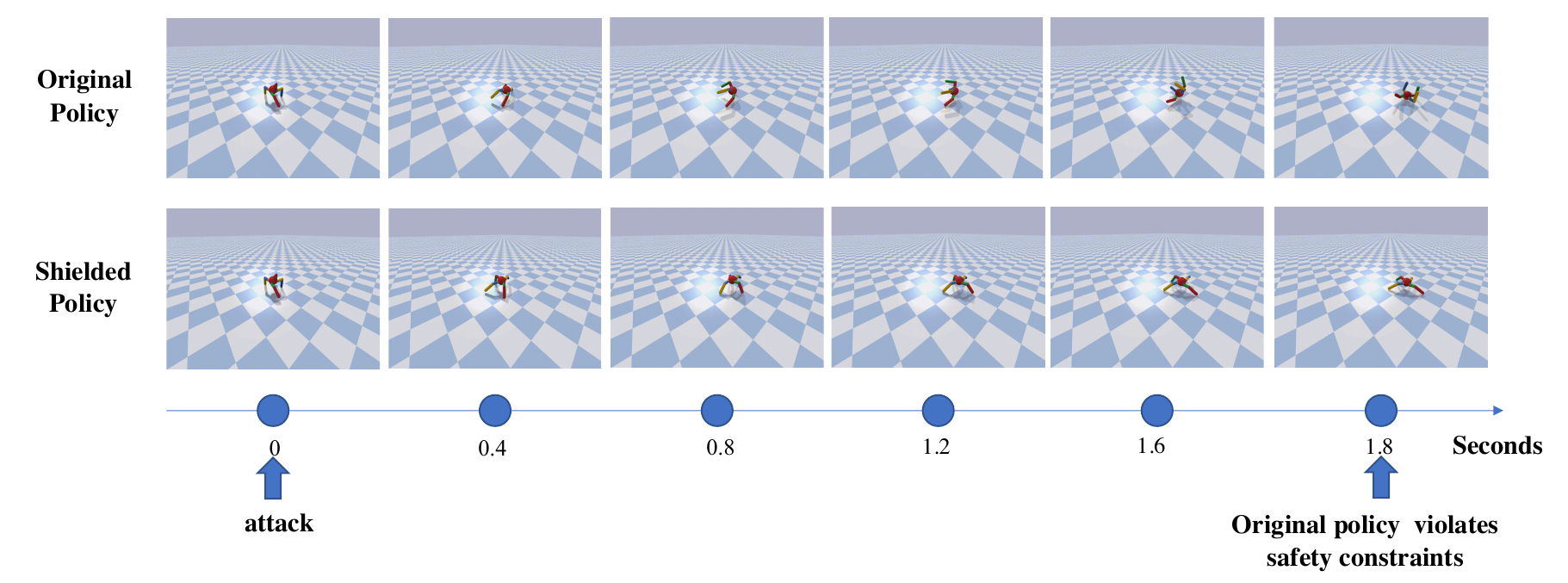
Our contributions are three-fold:

1. We present an adversarial testing framework that identifies natural unsafe states found near safe ones in a simulated trajectory of learning-enabled controllers. The RL controller is guaranteed to produce trajectories that lead to a safety violation from these states.

2. We learn detector classifier from these unsafe trajectories that precisely classify safe and unsafe states, and auxiliary policies triggered when the detector identifies an unsafe state; applying a shield on a presumed unsafe state yields a new safe trajectory, i.e., a trajectory that satisfies desired safety properties.

3. We provide a detailed experimental evaluation over a range of well-studied RL benchmarks, including the PyBullet suite of robotic environments and the F16 ground collision avoidance system. Our results justify our claim that the robustness of black-box RL-enabled controllers can be significantly enhanced using learning-based detection and shielding approaches, without noticeable loss in performance.

Our overarching goal in this paper is to overcome inherent deficiencies in RL policies that do not account for environment conditions which can be maliciously or unintentionally perturbed. These conditions potentially comprise a large attack surface, but in the black-box setting we consider here, fine-tuning the model is not possible. Our approach thus provides a meaningful pathway to identify and mitigate attacks that exploit unrecognized weaknesses of the deployed model, resulting in learning-enabled RL controllers that provide much higher degrees of assurance than the state-of-the-art, without requiring re-training or white-box analysis.

The remainder of the paper is organized as follows. In the next section, we present some relevant background material. Section 3 formalizes the problem we consider and our goals. Section 4 presents details about our approach. Experimental results are given in 5. Related work and conclusions are presented in Sections 6 and 7.

2 Background

Optimum Policies for Discrete-time Continuous Systems

We consider discrete-time systems $M=\langle S,A,f,R\rangle$ with non-linear dynamics $f$, continuous state space $S\subseteq\mathbb{R}^{n}$ and action space $A\subseteq\mathbb{R}^{k}$. Here $s_{t+1}=f(s_{t},u_{t})$ where $s_{t}\in S$ is the state at time step $t$ and $f$ is a complex unknown non-linear function. The objective, given a reward function $R:S\times A\rightarrow\mathbb{R}$, is to find a policy $\pi:S\rightarrow\Delta(A)$ where $\Delta(A)$ is a probability distribution over $A$ that maximizes the discounted return $\mathbb{E}_{\pi,S_{o}}[\underset{t=0..T}{\sum}\gamma^{t}R(s_{t},a_{t})]$ where $\gamma\in(0,1)$ is the discount factor and $S_{o}$ is the initial state space. Given a policy $\pi$ a trajectory $\tau=(s_{0},...,s_{T})$ is the sequence of states obtained when $s_{t+1}=f(s_{t},\pi(s_{t}))$ up to a horizon $T$.

Bayesian Optimization

Bayesian optimization (BO) is a black-box optimization approach which aims at finding the global minimum for a black-box function $F(x)$ by querying a constrained number of times. This constraint is motivated by the expectation that evaluating the objective function often requires significant computational resources. BO models $F(x)$ with a prior (frequently Gaussian Process-based) and uses an acquisition function to query values of $F(x)$ while trading off exploration and exploitation.

3 Problem Statement

Consider a continuous-state system $M$ where user-defined safe ($S_{s}$) and unsafe states ($S_{u}$) form a partition over the entire state space $S$ of $M$. A rollout of a trained agent policy $\pi_{o}$ on $M$ yields a state trajectory $\tau_{o}=(s_{0},...,s_{T})$. Let $\mathcal{T}(\pi_{o},M,S_{o})$ be the set of safe trajectories formed by rollouts of policy $\pi_{o}$ in the system $M$ with initial state space $S_{o}$ (i.e. trajectories in this set do not contain any states in $S_{u}$).

We consider the state dimensions which are used for computing the input of the agent policy $\pi_{o}$. These are often related to spatial characteristics such as joint position, angle, velocity, and robot center of mass. Define a filter $\phi(s)$ that yields a subset of modifiable state dimensions. Applying $\phi(s)$ to a trajectory $\tau$ yields $\phi(\tau)=(\phi(s_{0}),...,\phi(s_{T}))$.

Define a $\epsilon$-state perturbation of a state $s$ on the filtered dimensions in $\phi(s)$ to be another state $s^{\prime}\in S$ that is within $\epsilon$ distance away from $s$ by varying the set of dimensions in $\phi(s)$. We choose the $L_{\infty}$ norm to measure state distances. Given a state $s$, denote $P_{\epsilon}(s)$ to be the set of all possible perturbations on $s$.

Function Shield($state$):

       Given detector, $\pi_{o}$, $\pi_{\mathit{aux}}$

      if detector ($state$) then

             return $\pi_{\mathit{aux}}$

            

      else

             return $\pi_{o}$

            

       end if

      

Algorithm 1 Shield Defense Outline

We define an Adversarial State Attack $\texttt{Att}_{\epsilon}(\tau_{o})$ to be a set of states in which each state $s\in\texttt{Att}_{\epsilon}(\tau_{o})$ is an $\epsilon$-state perturbation on a state in the trajectory $\tau_{o}$ that causes the new trajectory to be unsafe. In other words, $s\in\texttt{Att}_{\epsilon}(\tau_{o})$ if, for some $k$ and $s^{\prime}$, $0\leq k\leq T$, $s^{\prime}\in P_{\epsilon}(s_{k})$, and executing the policy $\pi_{o}$ from $s^{\prime}$ leads to a state in $S_{u}$. This can be thought of as a state perturbation at an arbitrary time index along the trajectory that results in safety failure. These perturbations can be minute, a small shift of a robot due to a bump on the ground, or mild turbulence affecting the positioning of a jet in midair. If $\epsilon$ is unconstrained, perturbations can be unrealistic, unlikely to occur in practice, or impossible to defend against given existing environment transition dynamics. We thus concern ourselves with values of $\epsilon$ that lead to perturbed states in Section 5.1.

We aim to find a way to defend against adversarial state attacks leading to a more robust control strategy that is still performant. In real-world black-box scenarios, we have no access to both controller internals (underlying control policy) and environment conditions. Thus, an effective defense must treat the original policy $\pi_{o}$ as a black box and make no assumptions about the (hidden) environment dynamics. With these constraints in mind, we divide this problem into two stages. The first step is to detect adversarial state attacks, knowledge of which can be used to act differently, by shielding $\pi_{o}$ from malicious state perturbations (the second step).One defense outline is in the style of [1] where a shield modulates actions taken by $\pi_{o}$ based on the observation provided by the environment. We structure a simple two-level function to represent the shield shown in Algorithm 1. The upper level would be able to detect that an $\texttt{Att}_{\epsilon}$ attack has occurred while the lower level would be a policy to bring the system back to a safe state. We call the upper level function the detector and the lower level policy the auxiliary policy ($\pi_{\mathit{aux}}$).

With this setup, the constructed defense then uses the detector to decide whether to follow the original policy $\pi_{o}$ or switch to $\pi_{\mathit{aux}}$. If these two functions are accurate, this approach is robust to adversarial state attacks for a given $\epsilon$. Our goal is thus to learn these two functions keeping in mind the restrictions placed on the defense scheme.

4 Approach

Based on the definition of Adversarial State Attack $\texttt{Att}_{\epsilon}$ (Section 3), given a trained policy $\pi_{o}$, a system $M$ with some initial states $S_{o}$, we aim to find a set of state-based adversarial attacks $\texttt{Adv}_{\epsilon}(\pi_{o},M,S_{o})$ defined as:

$$\texttt{Adv}_{\epsilon}(\pi_{o},M,S_{o})=\{s\ |\ {s\in\texttt{Att}_{\epsilon}(\tau)}\wedge\tau\in\mathcal{T}(\pi_{o},M,S_{o})\}$$

Our defense strategy follows the outline described in Algorithm 1.

4.1 Safety Specifications

Similar to [8], we consider a safety specification $\varphi$ consisting of multiple predicates denoted as $\rho$ connected using Boolean operators including conjunction and disjunction:

$$\varphi:=\rho\ |\ \varphi\wedge\varphi\ |\ \varphi\vee\varphi\ \ \ \ \rho:=t=t^{\prime}\ |\ t\neq t^{\prime}\ |\ t\leq t^{\prime}\ |\ t<t^{\prime}\ |\ t\geq t^{\prime}\ |\ t>t^{\prime}$$

A term $t$ is any real-valued function defined over system variables. For example, consider a robot with the height of the center of mass being $z$. One safe height specification $\varphi_{\mathit{safe}}$ is $z_{\mathit{safe}}<z$ where $z_{\mathit{safe}}$ is a height threshold.

4.2 Attack

The search problem for $\texttt{Adv}_{\epsilon}(\pi_{o},M,S_{o})$ as defined above is in general intractable. We thus require a more precise objective that is easy for optimization. To tractably find $\texttt{Adv}_{\epsilon}(\pi_{o},M,S_{o})$, we define a safety reward function $L(\varphi):S\rightarrow\mathbb{R}$ for $M$. A key feature of $L(\varphi)$ is that, given a state $s\in S$, $\varphi$ holds on $s$ iff $L(\varphi)(s)>0$. We define $L(\rho)$ recursively. First, $L(t<t^{\prime}):=t^{\prime}-t$. For the above robot example, $L(\varphi_{safe}):=z-z_{safe}$. We have $L(t=t^{\prime}):=\delta[t=t^{\prime}]$ where $[\cdot]$ is an indicator function and $\delta$ is a user-configurable constant, $L(t\neq t^{\prime}):=L(t<t^{\prime}\vee t>t^{\prime})$, and $L(t\leq t^{\prime}):=L(t<t^{\prime}\vee t=t^{\prime})$. $L(\varphi)$ is also recursively defined: $L(\varphi\wedge\varphi^{\prime}):=\min(L(\varphi),L(\varphi^{\prime}))$ and $L(\varphi\vee\varphi^{\prime}):=\max(L(\varphi),L(\varphi^{\prime}))$.

Given a trajectory $\tau$, its safety reward is

$$L(\varphi)(\tau)=\underset{s\in\tau}{\min}\ L(\varphi)(s)$$

Attack setup

With $L(\varphi)$ defined above as an effective proxy for safety measurement, given a (set of) trajectory $\tau$ of a system $M$ from $S_{o}$ i.e. $\tau\in\mathcal{T}(\pi_{o},M,S_{o})$, we search in $\underset{s\in\tau}{\bigcup}{P_{\epsilon}(s)}$ a set of state $S^{\prime}$ with the objective of minimizing the safety reward $L(\varphi)(\tau^{\prime})$ where $\tau^{\prime}\in\mathcal{T}(\pi_{o},M,S^{\prime})$. Observe that $L(\varphi)(\tau^{\prime})$ is essentially a function over states (parameterized by the first state of $\tau^{\prime}$ and the policy $\pi_{o}$). The ability of Bayesian Optimization (BO) in optimizing black-box functions (e.g. $L(\varphi)(\tau^{\prime})$) makes it qualified as an optimization scheme for our purpose. We thus use BO to find states in $\texttt{Adv}_{\epsilon}(\pi_{o},M,S_{o})$ that lead to trajectories with a negative $L(\varphi)$ reward and hence unsafe. In our experiments, we use EI (Expected Improvement) [14] as the acquisition function and GP (Gaussian Processes) [20] as the surrogate model.

Feature Selection

Naïve BO does not scale with the dimensionality of a controller’s feature space. One way to improve scalability is to optimize over a reduced set of features. For example, Ghosh et al. [8] used REMBO [25] to create a reduced input space. We apply feature selection using a 2-stage approach. First, we run BO attacks without feature selection and collect unsafe and safe trajectories. We then train a random forest with the collected data, selecting the top-$k$ features based on a mean decrease in impurity i.e. refining the filter operator $\phi$ in Sec. 3. We rerun the attack on these features again, searching for more unsafe trajectories.

4.3 Defense

Training the Detector

Our defense approach must be aware of potential unsafe states that occur when using the original policy $\pi_{o}$. To this end, we train a classifier (the detector) with data derived during the attack phase. When we attack policy $\pi_{o}$ with BO, we obtain batches of trajectories via simulation in the environment, some of which starting from states in $\texttt{Adv}_{\epsilon}(\pi_{o},M,S_{o})$ are unsafe, and others are safe. For a safe trajectory, we label all included states as safe, while for an unsafe trajectory $\tau$, all states that follow a state found in $\texttt{Att}_{\epsilon}(\tau)$ are labelled as unsafe. Training a classifier with this data yields a detector that differentiates between states that are safe from those that produce unsafe trajectories affected by states in $\texttt{Adv}_{\epsilon}(\pi_{o},M,S_{o})$.

Auxiliary Policy

When running a system, we use the detector to monitor current system states. If the detector identifies a potentially vulnerable state, the defense strategy must yield an alternative action (sequence) to prevent the agent from entering an unsafe region. The auxiliary policy should be able to defend against attacks in $\texttt{Att}_{\epsilon}$. To obtain the final building block of our defense, we use the trained detector to provide a reward signal for training an auxiliary policy ($\pi_{\mathit{aux}}$) with PPO [21] and DDPG [23].

Specifically, we train $\pi_{\mathit{aux}}$ on a slightly modified version of $M$, $M^{\prime}=\langle S,A,f,R_{M^{\prime}}\rangle$. The reward function $R_{M^{\prime}}$ has two components:

1. We integrate the detector as a part of the reward function to train the auxiliary policy. We choose a simple reward signal based on the detector output. For an input state of the reward function, if the detector finds the state safe, the action is given a reward 1 and otherwise a reward 0 is given. We call it detector reward. This reward component aims to bring the agent into a safe state identified by the detector.

2. The safety reward defined in Sec. 4.2 is also an indicator of safety. A straightforward way to use this information is to add it as well to the reward signal for training the auxiliary policy. Optimizing the safety reward of each rollout maximizes policy safety. This reward component encourages $\pi_{\mathit{aux}}$ to behave safely.

Deployment of the defense

Intuitively, $\pi_{\mathit{aux}}$ only focuses on safety and does not care about performance. Running the original policy $\pi_{o}$ in tandem with $\pi_{\mathit{aux}}$ (Algorithm 1) can retain performance provided by $\pi_{o}$ while ensuring safety provided by $\pi_{\mathit{aux}}$.

5 Experiments

PyBullet

A number of our experiments are conducted in PyBullet [5], a well-studied open-source suite of robotic environments. The specific environments tested on were the Ant, HalfCheetah, Hopper and Humanoid robots. The objective of each of these environments is to stay upright and sustain forward motion. The robots are modeled using the velocity, orientation, and position of their joints. For example, Ant’s 8-D action space is used to control each individual motor while navigating its 29-D state space. Its observation has 28 dimensions consisting of 4 dimensions of feet contact information, and 24 dimensions of joint information with body location and velocity. Its primary safety constraint is to remain upright; additional details are provided in Appendix A.3. For more details of the environments, one may refer to the models’ XML definition in the PyBullet repo . For the attacked policy, we used an open-source implementation of popular RL algorithms [12] with the saved models provided which are trained on stochastic versions of the environment (to simulate sensor noise).

F16 Ground Collision Avoid System

The F16 environment is a model of the jet’s navigation control system[11]. The F16 is modeled with 16 variables and with non-linear differential equations as dynamics. The safety constraints are provided based on the aircraft flight limits and boundaries of the model. Our objective is to keep the jet level and flying within the specified constraints. Further details on the state dimensions, initialization and safety bounds are given in Appendix A.2. The attacked policy of this model is trained with PPO.

Classic Control Environments

In addition to the above environments, we include several classical control benchmarks including (Inverted) Pendulum, $n$-Car platoon and large helicopter. The (Inverted) Pendulum’s goal is to swing a pendulum to vertical. $n$-Car platoon models multiple ($n$) vehicles forming a platoon maintaining a safe distance relative to one another [22]. Large helicopter [7] models a helicopter with 28 variables and has constraints on each variables. These benchmarks’ constraints are provided in Appendix A.1. We trained the Helicopter with DDPG while the other models use the pretrained DDPG [23] policies given in [27].

5.1 Evaluation

Benchmarks	dims (obs/state)	simu. traj. length	Attack $\varepsilon$	rand. attack	BO attack	defense succ. rate	attack improvement using shielded policy
Hopper-a2c	15/12	1000	0.001	1.29%	2.18%	91.40%	43.51%
Hopper-ppo				0.41%	5.27%	97.80%	27.97%
Hopper-trpo				1.71%	1.97%	97.90%	48.16%
HalfCheetah-a2c	26/17	1000	0.02	0.36%	9.43%	91.40%	34.46%
HalfCheetah-acktr				0.90%	14.54%	92.80%	65.23%
HalfCheetah-ddpg				1.63%	11.84%	88.20%	67.27%
HalfCheetah-ppo2				0.38%	4.68%	97.80%	50.53%
HalfCheetah-sac				4.40%	5.88%	97.90%	62.12%
HalfCheetah-trpo				0.77%	4.83%	97.90%	49.02%
Ant-a2c	28/29	1000	0.0075	0.17%	1.26%	82.60%	66.20%
Ant-ddpg				0.42%	4.43%	94.30%	93.57%
Ant-ppo				1.47%	11.78%	88.70%	91.39%
Ant-sac				2.82%	14.83%	96.00%	94.02%
Ant-td3				5.79%	12.79%	93.60%	72.52%
Humanoid-ppo	44/47	1000	0.001	0.38%	2.00%	91.90%	22.93%
Pendulum-ddpg	2/2	200	*	0.03%	8.72%	100.00%	100.00%
4carploon-ddpg	7/7	1000	*	0.01%	3.82%	100.00%	94.71%
8carploon-ddpg	15/15	2000	*	0.72%	4.13%	100.00%	100.00%
Helicopter-ddpg	28/28	2000	*	0.00%	0.26%	100.00%	100.00%
F16-ppo	8/16	2000	*	0.01%	2.60%	96.40%	96.69%

* Use allowed variance of initial state which is given by the benchmark itself

Table 1: Experimental Results. Benchmarks are of the form, E-A where E is the Environment and A is the type of controller attacked.

Selecting Attack Range

As mentioned in Sec. 3, an Adversarial State Attack $\texttt{Att}_{\epsilon}$ requires a meaningful $\varepsilon$-state perturbation. We choose $\varepsilon$ with following strategy. For a specific robot in the PyBullet benchmarks, we initialized our $\varepsilon$ to be 0.001. We randomly perturbed initial states and run simulations 1000 times for every available policy. If there is a policy that does not find any unsafe states, we increase $\varepsilon$ by 0.0005, and repeat this process until unsafe states are found in all policies. We believe this is a sensible strategy because none of these benchmarks are equipped with constraint specifications that indicate the range of acceptable states that can be generated by the environment. For all the other benchmarks, constraints on these ranges were available and used directly.

Attack Results

Figure 2: Attack success rate for Humanoid-ppo under different feature dimension reduction percentages.

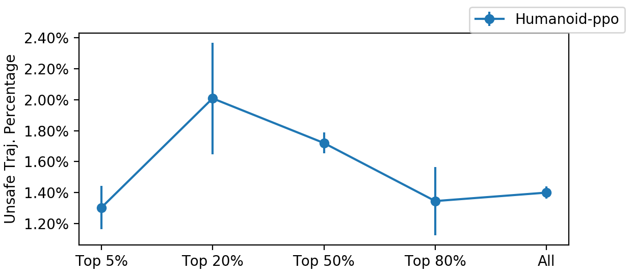
Table 1 shows two attack strategies. The first, rand. attack indicates the percentage of safety violations detected when initializing the state randomly around a sampled trajectory with respect to the chosen $\varepsilon$. For each benchmark, we randomly sampled 40K states within the bounds determined by $\varepsilon$ and initialized the simulations accordingly. Column BO attack shows the attack success rate when using BO to discover attacks. The GPs of the method are initialized with 10 randomly sampled states and the BO algorithm samples the safety reward 30 times. For each state in one trajectory, we generate 40 sampled trajectories. If the length of an attacked trajectory was $L$, $40\times L$ trajectories would be collected in one attack. We then count the unsafe trajectories in these simulations. For high-dimensional benchmarks like Humanoid, our attack focused on the top 20% most important features (9 features); these features were selected using the approach described in 4.2. With this feature reduction in place, our technique achieves an average 2% attack success rate, compared to just a 0.38% success rate using a randomized attack strategy. Results for other dimension reduction choices are given in Figure 2.

Defense Results

We trained detectors with the states generated by our attack and learned auxiliary policies with the detector and corresponding safety reward. We measured the quality of our defense in two ways. First, we want to know how successful our detector and auxiliary policies are in preventing attacks on the original policy that would otherwise lead to a safety violation. Second, given a shielded policy, i.e., a policy that integrates the original, defense, and auxiliary policy, we measure how effective this combined policy is in reducing the number of unsafe states available to an attack, compared to the original policy.

To answer the first question, we run BO attacks on the original policy, employing our detector and shield policy to detect and avoid unsafe trajectories. Note that we may still find unsafe trajectories because not all attacks are necessarily preventable for reasons discussed below. The defense success rate on the PyBullet benchmarks ranges from 82.6% to 100%. On the simpler classical control benchmarks, the defense success rate can achieve 100% while the F16GCAS benchmark has a 96.4% defense success rate. These results support our claim that $\varepsilon$-state perturbations used in adversarial attacks in these environments can be effectively mitigated. We note that our defense method does not provide verifiable guarantees of safety. There are two primary reasons for this: a) the possible existence of states in our attack which are not recoverable by any policy (eg: a robot whose forward momentum will cause it to fall regardless of any possible shield action that may be taken); and, b) covariate shift due to our black-box setting that does not provide insight into environment dynamics, making it impossible to provide guarantees on detector accuracy during testing since the detector and auxiliary policy are trained only with the adversarial states discovered by previously seen BO attacks. In other words, even if the detector is accurate, it is also untenable to assert that the auxiliary policy ($\pi_{\mathit{aux}}$) trained by RL is always reliable due to variations while training.

The attack improvement using shielded policy column shows the percentage reduction in unsafe states discovered by a BO attack when applied to the shielded policy as compared to the original. The trajectories admitted by the shielded policy are more constrained than the original since the policy is derived as a mixture of both the original and the auxiliary (safety) policy. Consequently, we would expect a fewer number of unsafe states to be discoverable under this new policy when compared against a policy in which safety was not taken into account. Indeed, the results shown in the column justify this intuition. For all benchmarks, the use of a shielded policy reduces the number of unsafe states found by a BO attack by at least 22.93%. The use of this blended policy on the three Classical Control tasks demonstrates 100% empirical robustness, while the F16 benchmark is very close behind at 96.69%. Several of the PyBullet benchmarks such as Ant-ddpg and Ant-sac show similar improvement.

Figure 3: Average Reward for Original Policy and Shielded Policy

Performance of the Shielded Policy

The experiments in Figure 3 investigate the impact of considering safety (and thus shield interventions) on performance. We randomly initialized the simulation around the attacked trajectory within a range bounded by $\varepsilon$. For each benchmark, we run a simulation 1000 times and count the (normalized) average return yielded with the original policy and shielded policy. The y-axis is the trajectory return scaled by a constant shared among each environment’s benchmarks. It represents the performance of the corresponding policy(i.e., moving fast with low electricity cost). The result in Figure 3 supports our claim that the cost of shield interventions is typically modest, on average only 5.78% variance compared to the performance exhibited by the original.

6 Related Work

As discovered in [13], by adding tiny or even invisible perturbations to inputs at each time-step, neural network RL policies are vulnerable to adversarial attacks, which can lead to abnormal system behavior and significant performance drop. Simple generation algorithms such as fast gradient sign method (FSGM) [10] can craft adversarial examples for some RL algorithms that are less resistant to adversarial attack. However, our approach can effectively attack a wide range of modern RL algorithms. In the black-box setting where gradient information is not available, [4] proposed a policy induction attack that exploits the transferability of adversarial examples [24]. To attack, it obtains adversarial state perturbations from a replica of the victim’s network, e.g. using FSGM, and trains the replica to simulate the victim’s network. In contrast, our approach does not attempt to replicate the victim’s network but uses Bayesian optimization and dimension reduction to approximate only part of the search space that is relevant to insecure model behavior. [15] also proposed to find adversarial attacks in the black-box setting. It pushes the RL agent to achieve the expected state under the current state by generating adversarial perturbations from action sequence planning enabled by model-based learning. As opposed to this approach, our work is model-free as we do not need to learn an environment model to guide the search of adversarial examples. While using Bayesian optimization for crafting adversarial examples was previously explored in [8], that work focuses on environment parameters such as initial and goal states. Our work exploits Bayesian optimization to attack at various time-steps in a rollout. In [9], the attacker solves an RL problem to generate an adversarial policy creating natural observations and acting in a multi-agent environment to defeat the victim policy. The setting of our problem is substantially different as we assume the input distribution to the victim policy is not significantly changed at test time to better mirror realistic behaviors. Importantly, our technique differs from these previous approaches by training an auxiliary policy to shield and defend the victim network.

To defend an RL policy, prior work has applied adversarial training to improve the robustness of deep RL policies. Adversarial RL training fine-tunes the victim policy against adversary policies by exerting a force vector or randomizing many of the physical properties of the system like friction coefficients [17, 19, 16, 18]. The trained policy can robustly operate in the presence of adversarial polices that apply disturbance forces to the system. Defenses based on this idea also generalize to multi-agent RL environments [9] which shows that repeated fine-tuning can provide protection to a victim policy against a range of adversarial opponents. Our approach differs from these techniques because we consider black-box settings, and do not attempt to fine-tune the internals of a victim policy. Instead, a shield-based auxiliary policy is trained to improve the victim policy’s resistance to adversarial perturbations. There exists recent work that synthesizes verified shields to protect RL policies leveraging formal methods  [27, 3, 26]. However, unlike our approach, these techniques do not scale to high-dimensional environment and adversarial disturbances.

7 Conclusions

Learning-enabled controllers for CPS systems are subject to adversarial attacks in which small perturbations to the states generated by an environment in response to a controller’s actions can lead to violations of important safety conditions. In this paper, we present a new framework that uses directed attack generation to learn defense policies that accurately differentiate between safe and unsafe states and an auxiliary shielding policy that aims to recover from an unsafe state. Notably, our methodology operates in a completely black-box setting in which environment dynamics are unknown. Experimental results demonstrate our approach is highly effective over a range of realistic sophisticated controllers, with only modest impact on overall performance.

8 Broader Impact

Machine learning has demonstrated impressive success in a variety of applications relevant to the core thrust of this paper. In particular, autonomous systems such as self-driving cars, UUVs, UAVs, etc. are examples of the kind of learning-enabled CPS systems whose design and structure are consistent with the applications considered here. These systems are characterized by intractably large state spaces, only a small fraction of which are explored during training. Because the space of possible environment actions is so large, it is unrealistic to expect that the environment models learnt used to train these controllers represent all possible behaviors likely to be observed in deployment. These covariate shifts can affect controller behavior resulting in violations of important safety constraints. These violations can have significant negative repercussions in light of the common use case for these applications which often involves operating in environments with high levels of human activity. Our shielding policy shows significant benefit in improving controller safety without requiring expensive retraining post-deployment.

Appendix A Benchmark Constraints

We present the initial constraints and safety constraints for all benchmarks in this section.

A.1 Classical Control

The classical control benchmarks and pretrained models come from [27]. Initial and safety constraints are in table 2.

Table 2: Classical Control Benchmarks

Benchmarks	Initial Constraints	Safety Constraints
Pendulum	$-0.3<x_{i}<0.3$, for $0\leq i\leq 1$	$-0.5<x_{i}<0.5$, for $0\leq i\leq 1$
4CarPloon	$-0.1<x_{i}<0.1$, for $0\leq i\leq 6$	$-2<x_{0}<2$, $-0.5<x_{1,3,5}<0.5,$ $-0.35<x_{2}<0.35$, $-1<x_{4,6}<1$
8CarPloon	$-0.1<x_{i}<0.1$, for $0\leq i\leq 14$	$-2<x_{0}<2,-0.5<x_{1,3,5,7,9,11,13}<0.5$, $-1<x_{2,4,6,8,10,12,14}<1$
Helicoptor	$-0.002<x_{i}<0.002$, for $0\leq i\leq 7$ $-0.0023<x_{i}<0.0023$, for $8\leq i\leq 27$	$-10<x_{13}<10$, $-9<x_{14}<9$ $-8<x_{i}<8$, for $0\leq i\leq 27\land i\neq 13,14$

A.2 F16GCAS

The F16GCAS benchmark is modelled with 16 variables. The meaning of each, along with initial space and constraints are shown in Table 3. When the initial space is 0, this variable is always initialized with 0.

Table 3: F16 Ground Collision Avoidance System

Variables	Meanings	Initial Space	Safety Constraints	Units
$V$	Airspeed	[491, 545]	[300, 2500]	ft/s
$\alpha$	Angle of attach	[0.00337, 0.00374]	[-0.1745, 0.7854]	rad
$\beta$	Angle of side-slip	0	[-0.5236, 0.5236]	rad
$\phi$	Roll angle	[0.714, 0.793]	(-inf, inf)	rad
$\theta$	Pitch angle	[-1.269, -1.142]	(-inf, inf)	rad
$\psi$	Yaw angle	[-0.793, -0.714]	(-inf, inf)	rad
$P$	Roll rate	0	(-inf, inf)	rad/s
$Q$	Pitch rate	0	(-inf, inf)	rad/s
$R$	Yaw rate	0	(-inf, inf)	rad/s
$p_{n}$	Northward displacement	0	(-inf, inf)	ft
$p_{e}$	Eastward displacement	0	(-inf, inf)	ft
$h$	Altitude	[3272, 3636]	[0, 45000]	ft
$pow$	Engine thrust	[8.18, 9.09]	(-inf, inf)	lbf
$\int N_{z_{e}}$	Integral of down force error	0	[-3, 15]	g’s
$\int P_{s_{e}}$	Integral of stability roll rate error	0	[-2500, 2500]	rad
$\int(N_{y}+r)_{e}$	Integral of side force & yaw rate error	0	(-inf, inf)	mixed

A.3 Pybullet

For initial constraints, one may refer to $\mathtt{robot\_locomotors.py}$ in the pybullet repo. The initial spaces of different joints are defined in the $\mathtt{robot\_specific\_reset()}$ function. Safety constraints are defined in the $\mathtt{alive\_bonus()}$ function in the same file. These constraints focus on 2 variables, the height $\mathtt{z}$ and the pitch $\mathtt{p}$ of the robot, as well as the joint contacts with the ground. When the $\mathtt{alive\_bonus()}$ returns a value that is smaller than 0, the agent violates these constraints and the simulation terminates immediately. We present the safety constraints in Table 4.

Table 4: PyBullet Benchmarks safety constraints

Benchmarks	Safety Constraints
Hopper	$\mathtt{z}>0.8$ $\land$ $\mathtt{|p|}<1$
HalfCheetah	$\neg contact(joint1,2,4,5)\land|\mathtt{p}|<1$
Ant	$\mathtt{z}>0.26$
Humanoid	$\mathtt{z}>0.78$

$\neg contact$ means that the joints do not contact with the ground.

Appendix B Attack Transferability

Transferability is a general property of many adversarial attacks. Recall that given a policy $\pi_{0}$ in a system $M$ with initial states $S_{0}$, an adversarial set $\texttt{Adv}_{\epsilon}(\pi_{0},M,S_{0})$ is discovered with a Bayesian Optimization (BO) attack. Now, considering another policy $\pi_{1}$ on the same system $M$, we wish to know what percentage of $\texttt{Adv}_{\epsilon}(\pi_{0},M,S_{0})$ is also an adversarial state for policy $\pi_{1}$. We call this the transferable ratios for the benchmark. Several policies trained with different RL algorithms are available on the Ant, HalfCheetah, and Hopper environments. We measured the adversarial transferability between these different policies trained for the same robot system. Figure 4 shows these results.

Figure 4: Attack transferability between a given robot’s policies. Each row is the adversarial state ratio of one adversarial state set on different policies. i.e, for Hopper, the row a2c, column ppo means $13\%$ of the adversarial state set of a2c are also adversary states for ppo. The diagonal is always $100\%$ because states of one policy’s adversary dataset are always unsafe for that algorithm. The numbers in the tables are the transferable ratios.

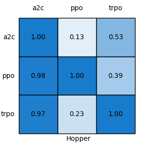
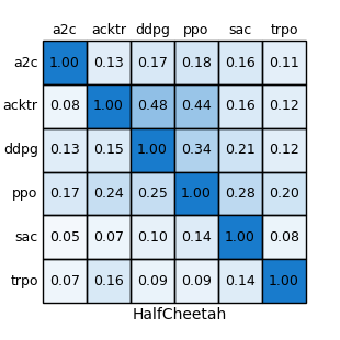
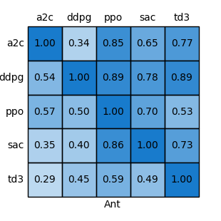
Because adversarial states can be transferred between different policies, the transferable ratio varies on different systems and policies. For HalfCheetah, adversarial states are less likely to be transferred into other policies when compared with Hopper and Ant. It is also true that an adversary state set can have a relatively high transferable ratio overall policies. For example, the adversarial state of Ant-ddpg(row) has greater than a $78\%$ transferable ratio on all policies. On the contrary, an adversary state set can also have a low transferable ratio for all policies excepted for its own as evidenced by HalfCheetah-sac(row). A policy can be vulnerable or resistant to the adversarial state of other policies. For example, Hopper-a2c(column) has $98\%$ and $97\%$ transferable ratio on adversarial states for ppo and trpo respectively, while the Hopper-ppo(column) has only $13\%$ and $23\%$ transferable ratio on adversarial states for a2c and trpo, respectively.

Appendix C Feature Importance

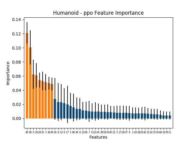
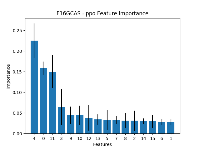
Not all features in an application are equally related to safety specifications. Taking the Humanoid robot as an example - its safety specification $\varphi$ is to stay upright ($z>0.78$). This goal is directly dependent on the height of the robot, thus the height feature is highly related to safety. By applying feature selection on the attack results, we can rank feature importance automatically. In our experiments, we selected the top-$20\%$ most important features to reduce the attack dimension (the dimension of filter $\phi$ defined in Section 4) of Humanoid-ppo. Their importance is marked as orange in Figure 5. We also analyzed the feature importance of the F16 Ground Collision Avoidance System in Figure 5. The top-$3$ important features related to the ground collision are airspeed, pitch angle, and attitude in order.

Figure 5: Humanoid-ppo & F16GCAS-ppo Feature Importance

Appendix D Shield Intervention Analysis

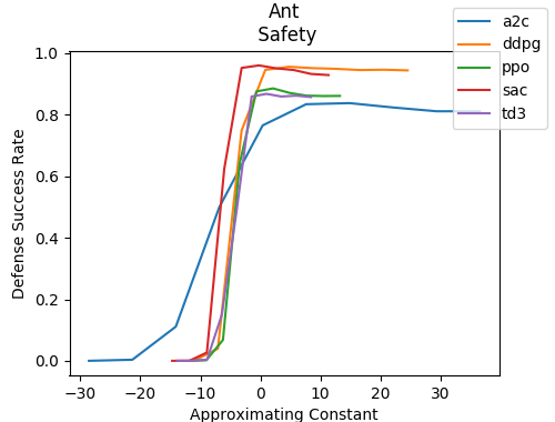
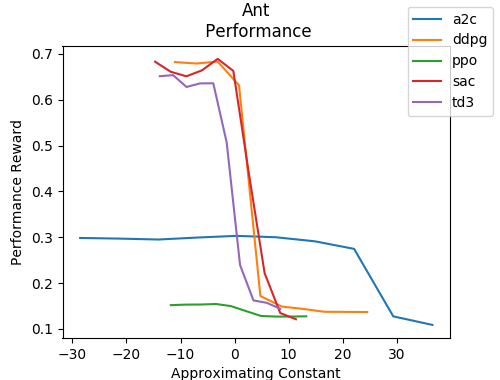
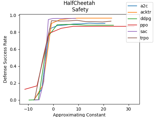
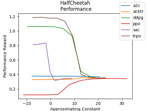
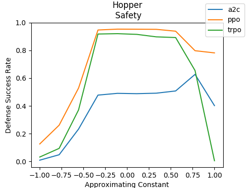
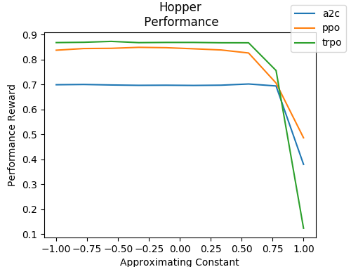
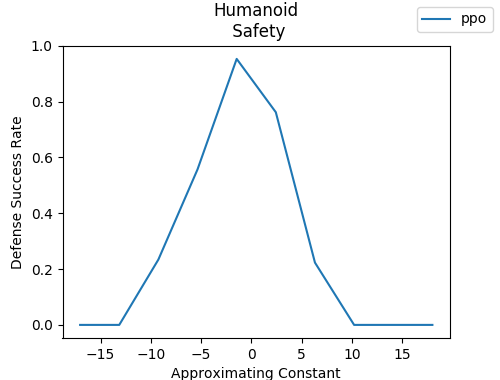
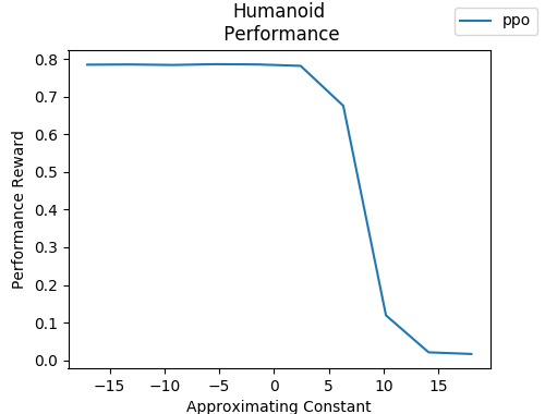
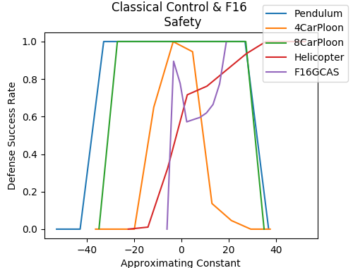
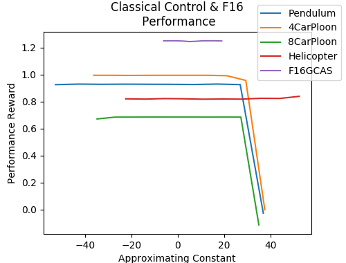
If the shield does not adequately intervene with the original policy, the original policy is vulnerable to states found in $\texttt{Adv}_{\epsilon}$. On the contrary, since our auxiliary policies are only trained to assist the original policy to be safe, too many shield interventions initiated by auxiliary policies can reduce the performance of the system. To measure the impact of shield interventions, we crafted experiments to control the number of interventions. Given an input state $s$, our detector gives scores to safe and unsafe labels, and outputs the label with the higher score. For state $s$, suppose the scores which the detector gives to the safe and unsafe labels are $S_{safe}(s)$ and $S_{unsafe}(s)$ respectively. In the general setting, if $S_{safe}(s)>S_{unsafe}(s)$, the detector marks $s$ as safe. Now, we change this setting as the detector can mark $s$ safe iff $S_{safe}(s)>S_{unsafe}(s)+C$. Otherwise, mark $s$ as unsafe. $C$ is an approximating constant - as it increases, more states will be marked as unsafe, thus there will be more shield interventions triggered by the auxiliary policy. For small values of C, more states will be marked as safe, and thus fewer shield interventions will be triggered.

Thus, by changing the value of the approximating constant, we can measure the relationship between defense success rates and shield interventions, as well as the relationship between performance and shield interventions. For the first case, we initialized our simulation with all the states in the adversarial state set $\texttt{Adv}_{\epsilon}(\pi_{0},M,S_{0})$ for original policy $\pi_{0}$. In this case, if there is no shield intervention, the system will violate the safety specification. For the second one, we measured the performance reward by initializing the system around one trajectory, which is the same setting as described in Section 5.1. We decide the range of the approximating constant with the detector training set derived from the attack phase. For each state $s$ in the training set, we calculated the difference $S_{safe}(s)-S_{unsafe}(s)$ and selected the smallest and largest difference as the lower bound $l$ and upper bound $h$ of the approximating constant. Given a sample range $[l,h]$, when $C>h$, all states in this set will be marked as unsafe; when $C<h$, all states in this set will be marked as safe. For each benchmark, we sample 10 approximating constant values in this interval equally separated.

We analyzed shielded policies on Ant in Fig 6. As the approximating constant $C$ increases, more interventions are involved and the defense success rate increases. However, the performance reward decreases dramatically due to these increasing interventions. The results on HalfCheetah are shown in Figure 7. Similar to Ant, as $C$ increases, the defense success rate also increases. For most policies, the performance reward decreases as $C$ increased, but when policies are not well-trained, such as PPO, the performance reward actually increases since the system becomes safer and thus the robot learns a more accurate reward. The results of Hopper and Humanoid are shown in Figure 8 and Figure 9, respectively. Unlike the results shown for Ant and Halfcheetah, we find that too many interventions can lead to unsafety. This is because the auxiliary policies are only trained to assist the original policy. As long as it can pull the system to safe states for the original policies, it can gain a decent reward. However, the auxiliary policy itself may not be a safe policy independently. On the other hand, if the number of interventions is small, the system is vulnerable to the following states in $\texttt{Adv}_{\epsilon}$. Our shielded policies perform best when $C$ is around 0 since the auxiliary policy is trained under the instruction of detector when $C$ is $0$. Similar to Ant and HalfCheetah, when $C>0$, the performance reward decreases as the number of interventions increases on Hopper and Humanoid. Results of classical control and F16GCAS benchmarks are in Figure 10. Excessive interventions on the (inverted) pendulum, $4$-carploon, and $8$-carploon can make the system unsafe and decrease performance reward. When interventions are infrequent, these applications become vulnerable to adversarial perturbations. Shielded policies worked best when $C$ is close to 0. For Helicopter and F16GCAS, more interventions lead to safer behavior without comprising performance.

Figure 6: Ant Shield Intervention Analysis

Figure 7: HalfCheetah Shield Intervention Analysis

Figure 8: Hopper Shield Intervention Analysis

Figure 9: Humanoid Shield Intervention Analysis

Figure 10: Classical Control & F16GCAS Shield Intervention Analysis

Appendix E Hyper-parameters

E.1 Attack Hyper-parameters

When running the Bayesian optimization attack, we used the same hyper-parameters for all benchmarks. The acquisition function is Expected Improvement (EI). The $\xi$ of EI is 0.01. We use Gaussian Process (GP) with Matern kernel as a surrogate model. The hyper-parameters of the Matern kernel use the default tuned values in the skopt library. Before approximating the initial state-reward function with GP, we randomly sample 10 points. We then evaluate the initial state-reward function with points gotten by optimizing on acquisition function 30 times.

E.2 Defense Hyper-parameters

The Hopper’s detectors are random forests. Each of them has 100 trees with 50 max depth. The other detectors are neural networks. The search categories of neural network detectors’ hyper-parameters are given in Table 5.

Table 5: Hyper-parameters of Neural Network Detector

Hyper-parameter	Search Categories
Network Structure	obs_dim x 128 x 128 x 128 x 2
Learning Rate	[1e-4, 1e-3]
Mini-batch Size	[64, 128, 256, 512, 1024]
Training Epoch	[5, 10, 20, 50]
Optimizer	Adam

The auxiliary policies of Hopper, HalfCheetah and Ant are trained with DDPG, while the Humanoid, classical control and F16GCAS benchmarks are equipped with PPO auxiliary policy. The search categories of the auxiliary policy are listed in table 6 and 7.

Table 6: Hyper-parameters of DDPG

Parameters	Search Categories
Actor Network Structure	obs_dim x 64 x 64 x action_dim
Critic Network Structure	obs_dim x 64 x 64 x 1
Discount Factor $\gamma$	[0.99, 0.999]
Update Rate $\tau$	[1e-3, 1e-4]
others	Default values

Table 7: Hyper-parameters of PPO

Parameters	Search Categories
Policy Network Structure	obs_dim x 128 x 128 x action_dim
Training Step	[1e5, 5e5, 1e6, 2e6, 4e6]
Clipping Range	[0.01, 0.05, 0.1, 0.2]
Discount Factor $(\gamma)$	[0.99, 0.999, 1]
Entropy Cocfficicnt	0.01
GAE $(\lambda)$	0.95
Gradient Norm Clipping	0.5
Learning Rate	[2.5e-3, 2.5e-4, 2.5e-5]
Number of Actors	[4, 8, 16]
Optimizer	Adam
Training Epochs per Update	[4, 10]
Training Mini-batches per Update	[4, 16, 64, 128]
Unroll Length/n-step	[64, 128, 256, 512, 1024]
Value Function Coefficient	0.5

References

- [1] Mohammed Alshiekh, Roderick Bloem, Ruediger Ehlers, Bettina Könighofer, Scott Niekum, and Ufuk Topcu. Safe reinforcement learning via shielding. In The Thirty-Second AAAI Conference on Artificial Intelligence (AAAI-18). URL http://arxiv.org/abs/1708.08611.
- Bansal et al. [2018] Trapit Bansal, Jakub Pachocki, Szymon Sidor, Ilya Sutskever, and Igor Mordatch. Emergent complexity via multi-agent competition. In 6th International Conference on Learning Representations, ICLR 2018, Vancouver, BC, Canada, April 30 - May 3, 2018, Conference Track Proceedings, 2018. URL https://openreview.net/forum?id=Sy0GnUxCb.
- Bastani [2019] Osbert Bastani. Safe reinforcement learning via online shielding. CoRR, abs/1905.10691, 2019. URL http://arxiv.org/abs/1905.10691.
- [4] Vahid Behzadan and Arslan Munir. Vulnerability of deep reinforcement learning to policy induction attacks. URL http://arxiv.org/abs/1701.04143.
- Coumans and Bai [2016–2019] Erwin Coumans and Yunfei Bai. Pybullet, a python module for physics simulation for games, robotics and machine learning. http://pybullet.org, 2016–2019.
- Dosovitskiy et al. [2017] Alexey Dosovitskiy, Germán Ros, Felipe Codevilla, Antonio López, and Vladlen Koltun. CARLA: an open urban driving simulator. In 1st Annual Conference on Robot Learning, CoRL 2017, Mountain View, California, USA, November 13-15, 2017, Proceedings, pages 1–16, 2017. URL http://proceedings.mlr.press/v78/dosovitskiy17a.html.
- [7] Goran Frehse, Colas Le Guernic, Alexandre Donzé, Scott Cotton, Rajarshi Ray, Olivier Lebeltel, Rodolfo Ripado, Antoine Girard, Thao Dang, and Oded Maler. SpaceEx: Scalable verification of hybrid systems. In Ganesh Gopalakrishnan and Shaz Qadeer, editors, Computer Aided Verification, volume 6806, pages 379–395. Springer Berlin Heidelberg. ISBN 978-3-642-22109-5 978-3-642-22110-1. doi: 10.1007/978-3-642-22110-1_30. URL http://link.springer.com/10.1007/978-3-642-22110-1_30. Series Title: Lecture Notes in Computer Science.
- [8] Shromona Ghosh, Felix Berkenkamp, Gireeja Ranade, Shaz Qadeer, and Ashish Kapoor. Verifying Controllers Against Adversarial Examples with Bayesian Optimization. In 2018 IEEE International Conference on Robotics and Automation (ICRA), pages 7306–7313. doi: 10.1109/ICRA.2018.8460635. URL http://arxiv.org/abs/1802.08678.
- Gleave et al. [2020] Adam Gleave, Michael Dennis, Cody Wild, Neel Kant, Sergey Levine, and Stuart Russell. Adversarial policies: Attacking deep reinforcement learning. In 8th International Conference on Learning Representations, ICLR 2020, Addis Ababa, Ethiopia, April 26-30, 2020, 2020. URL https://openreview.net/forum?id=HJgEMpVFwB.
- [10] Ian J. Goodfellow, Jonathon Shlens, and Christian Szegedy. Explaining and harnessing adversarial examples. URL http://arxiv.org/abs/1412.6572.
- Heidlauf et al. [2018] Peter Heidlauf, Alexander Collins, Michael Bolender, and Stanley Bak. Verification challenges in f-16 ground collision avoidance and other automated maneuvers. In ARCH@ ADHS, 2018.
- Hill et al. [2018] Ashley Hill, Antonin Raffin, Maximilian Ernestus, Adam Gleave, Anssi Kanervisto, Rene Traore, Prafulla Dhariwal, Christopher Hesse, Oleg Klimov, Alex Nichol, Matthias Plappert, Alec Radford, John Schulman, Szymon Sidor, and Yuhuai Wu. Stable baselines. https://github.com/hill-a/stable-baselines, 2018.
- [13] Sandy Huang, Nicolas Papernot, Ian Goodfellow, Yan Duan, and Pieter Abbeel. Adversarial attacks on neural network policies. URL http://arxiv.org/abs/1702.02284.
- Jones et al. [1998] Donald R Jones, Matthias Schonlau, and William J Welch. Efficient global optimization of expensive black-box functions. Journal of Global optimization, 13(4):455–492, 1998.
- [15] Yen-Chen Lin, Zhang-Wei Hong, Yuan-Hong Liao, Meng-Li Shih, Ming-Yu Liu, and Min Sun. Tactics of adversarial attack on deep reinforcement learning agents. In Proceedings of the Twenty-Sixth International Joint Conference on Artificial Intelligence, pages 3756–3762. International Joint Conferences on Artificial Intelligence Organization. ISBN 978-0-9992411-0-3. doi: 10.24963/ijcai.2017/525. URL https://www.ijcai.org/proceedings/2017/525.
- Mandlekar et al. [2017] Ajay Mandlekar, Yuke Zhu, Animesh Garg, Li Fei-Fei, and Silvio Savarese. Adversarially robust policy learning: Active construction of physically-plausible perturbations. In 2017 IEEE/RSJ International Conference on Intelligent Robots and Systems, IROS 2017, Vancouver, BC, Canada, September 24-28, 2017, pages 3932–3939. IEEE, 2017. doi: 10.1109/IROS.2017.8206245. URL https://doi.org/10.1109/IROS.2017.8206245.
- OpenAI et al. [2018] OpenAI, Marcin Andrychowicz, Bowen Baker, Maciek Chociej, Rafal Józefowicz, Bob McGrew, Jakub W. Pachocki, Jakub Pachocki, Arthur Petron, Matthias Plappert, Glenn Powell, Alex Ray, Jonas Schneider, Szymon Sidor, Josh Tobin, Peter Welinder, Lilian Weng, and Wojciech Zaremba. Learning dexterous in-hand manipulation. CoRR, abs/1808.00177, 2018. URL http://arxiv.org/abs/1808.00177.
- Pattanaik et al. [2018] Anay Pattanaik, Zhenyi Tang, Shuijing Liu, Gautham Bommannan, and Girish Chowdhary. Robust deep reinforcement learning with adversarial attacks. In Elisabeth André, Sven Koenig, Mehdi Dastani, and Gita Sukthankar, editors, Proceedings of the 17th International Conference on Autonomous Agents and MultiAgent Systems, AAMAS 2018, Stockholm, Sweden, July 10-15, 2018, pages 2040–2042. International Foundation for Autonomous Agents and Multiagent Systems Richland, SC, USA / ACM, 2018. URL http://dl.acm.org/citation.cfm?id=3238064.
- Pinto et al. [2017] Lerrel Pinto, James Davidson, Rahul Sukthankar, and Abhinav Gupta. Robust adversarial reinforcement learning. In Doina Precup and Yee Whye Teh, editors, Proceedings of the 34th International Conference on Machine Learning, ICML 2017, Sydney, NSW, Australia, 6-11 August 2017, volume 70 of Proceedings of Machine Learning Research, pages 2817–2826. PMLR, 2017. URL http://proceedings.mlr.press/v70/pinto17a.html.
- Rasmussen [2003] Carl Edward Rasmussen. Gaussian processes in machine learning. In Summer School on Machine Learning, pages 63–71. Springer, 2003.
- Schulman et al. [2017] John Schulman, Filip Wolski, Prafulla Dhariwal, Alec Radford, and Oleg Klimov. Proximal policy optimization algorithms. CoRR, abs/1707.06347, 2017. URL http://arxiv.org/abs/1707.06347.
- Schürmann and Althoff [2017] Bastian Schürmann and Matthias Althoff. Optimal control of sets of solutions to formally guarantee constraints of disturbed linear systems. In 2017 American Control Conference (ACC), pages 2522–2529. IEEE, 2017.
- Silver et al. [2014] David Silver, Guy Lever, Nicolas Heess, Thomas Degris, Daan Wierstra, and Martin Riedmiller. Deterministic policy gradient algorithms. In Eric P. Xing and Tony Jebara, editors, Proceedings of the 31st International Conference on Machine Learning, volume 32 of Proceedings of Machine Learning Research, pages 387–395, Bejing, China, 22–24 Jun 2014. PMLR. URL http://proceedings.mlr.press/v32/silver14.html.
- [24] Christian Szegedy, Wojciech Zaremba, Ilya Sutskever, Joan Bruna, Dumitru Erhan, Ian Goodfellow, and Rob Fergus. Intriguing properties of neural networks. In International Conference on Learning Representations. URL http://arxiv.org/abs/1312.6199.
- Wang et al. [2013] Ziyu Wang, Masrour Zoghi, Frank Hutter, David Matheson, and Nando De Freitas. Bayesian optimization in high dimensions via random embeddings. In Twenty-Third International Joint Conference on Artificial Intelligence, 2013.
- Wu et al. [2019] Meng Wu, Jingbo Wang, Jyotirmoy Deshmukh, and Chao Wang. Shield synthesis for real: Enforcing safety in cyber-physical systems. In 2019 Formal Methods in Computer Aided Design, FMCAD 2019, San Jose, CA, USA, October 22-25, 2019, pages 129–137, 2019. doi: 10.23919/FMCAD.2019.8894264. URL https://doi.org/10.23919/FMCAD.2019.8894264.
- [27] He Zhu, Zikang Xiong, Stephen Magill, and Suresh Jagannathan. An inductive synthesis framework for verifiable reinforcement learning. In Proceedings of the 40th ACM SIGPLAN Conference on Programming Language Design and Implementation - PLDI 2019, pages 686–701. ACM Press. ISBN 978-1-4503-6712-7. doi: 10.1145/3314221.3314638. URL http://dl.acm.org/citation.cfm?doid=3314221.3314638.