Distinguished correlation properties of Chebyshev dynamical systems and their generalisations

Jin Yan j.yan@qmul.ac.uk Christian Beck c.beck@qmul.ac.uk School of Mathematical Sciences, Queen Mary University of London, Mile End Road, London E1 4NS, UK
Abstract

We show that, among all smooth one-dimensional maps conjugated to an N𝑁N-ary shift (a Bernoulli shift of N𝑁N symbols), Chebyshev maps are distinguished in the sense that they have least higher-order correlations. We generalise our consideration and study a family of shifted Chebyshev maps, presenting analytic results for two-point and higher-order correlation functions. We also review results for the eigenvalues and eigenfunctions of the Perron-Frobenius operator of N𝑁N-th order Chebyshev maps and their shifted generalisations. The spectrum is degenerate for odd N𝑁N. Finally, we consider coupled map lattices (CMLs) of shifted Chebyshev maps and numerically investigate zeros of the temporal and spatial nearest-neighbour correlations, which are of interest in chaotically quantized field theories.

keywords:
Bernoulli shift, Chebyshev maps, higher-order correlation functions, spectrum of Perron-Frobenius operator, coupled map lattices (CMLs)
journal: Chaos, Solitons and Fractals

1 Introduction

Maps conjugated to a Bernoulli shift are a standard paradigm for modelling chaotic dynamics [1, 2, 3, 4, 5, 6, 7]. It is useful to introduce a generating partition and symbolic dynamics for such maps [5, 8]. In the symbol space, dynamics generated by these mappings corresponds to a shift of symbols, and from a statistical point of view the sequence of symbols is statistically independent, thus implying strong mixing properties for the map under consideration.

One may, however, ask further questions for maps conjugated to a Bernoulli shift, as some properties depend on the particular way how the map is conjugated to the shift, i.e. they depend on the function underlying the topological conjugation. An interesting question is about the structure of higher-order correlation functions of the iterates of the map [2, 3]. Given a map T:XX:𝑇𝑋𝑋T:X\to X with iterates xn+1=T(xn)subscript𝑥𝑛1𝑇subscript𝑥𝑛x_{n+1}=T(x_{n}) these higher-order correlation functions are defined as xn1xn2xnrdelimited-⟨⟩subscript𝑥subscript𝑛1subscript𝑥subscript𝑛2subscript𝑥subscript𝑛𝑟\langle x_{n_{1}}x_{n_{2}}\cdots x_{n_{r}}\rangle, where delimited-⟨⟩\langle\cdots\rangle denotes the expectation with respect to the (natural) invariant measure of the map. We assume that the average xndelimited-⟨⟩subscript𝑥𝑛\langle x_{n}\rangle is zero (if it is non-zero it can be just subtracted from the iterates). An interesting question is: which smooth map conjugated to a Bernoulli shift of N𝑁N symbols with average xn=0delimited-⟨⟩subscript𝑥𝑛0\langle x_{n}\rangle=0 is the “most random” one, in the sense that it has the largest number of tuples (n1,,nr)subscript𝑛1subscript𝑛𝑟(n_{1},\ldots,n_{r}) such that the higher-order correlation function is exactly zero?

In this paper we show that the answer is given by Chebyshev maps of N𝑁N-th order. These are conjugated to the shift of N𝑁N symbols by means of a cosine function, and have been subject of many previous papers [9, 10, 11, 12, 13]. We will show that any other conjugating function produces more higher-order correlations. So for example, the binary shift map, T(x)=2xmod1𝑇𝑥modulo2𝑥1T(x)=2x\mod 1 (with subtracted mean), has more non-vanishing higher-order correlations than the second-order Chebyshev map T(x)=2x21𝑇𝑥2superscript𝑥21T(x)=2x^{2}-1, which is topologically conjugated via a cosine function. We show that all higher-order correlations can be analytically understood by studying the solutions of a certain set of diophantine equations, which can be solved by a graph-theoretical method, for general N𝑁N.

We will generalize our considerations to shifted Chebyshev maps, defined as T(x)=cos(Narccosx+a)𝑇𝑥𝑁𝑥𝑎T(x)=\cos(N\arccos x+a), which are conjugated by the same cosine function. We will evaluate higher-order correlations in full generality for any a[π/2,0]𝑎𝜋20a\in[-\pi/2,0], and show that again a=0𝑎0a=0 yields the smallest possible skeleton of non-zero higher-order correlations. We will find a suitable topological conjugation for shifted Chebyshev maps, for particular values of a𝑎a and N𝑁N, which relates their dynamics to that of ordinary (a=0𝑎0a=0) Chebyshev maps.

Investigating the higher-order correlation structure is significant especially when generating “noise” in a stochastic differential equation by a smooth deterministic chaotic dynamics [13, 14, 15, 16]. Clearly, the mathematical construction of Gaussian white noise that drives a stochastic differential equation possesses no correlations at all in time, but one may ask what type of higher-order correlations are generated by a smooth deterministic chaotic system at a microscopic level. Since the dynamics is deterministic and discrete there must be correlations even for maps conjugated to a Bernoulli shift: only the symbols that are shifted are statistically independent, but the iterates itself are not. We show that Chebyshev systems have least non-vanishing higher-order correlations when calculated with respect to their invariant measure, and are in this sense as close to white noise as possible for a smooth one-dimensional chaotic dynamics.

It is important to emphasise smoothness here. For example, a random number generator is not a smooth function of its seed variable. The question of the ultimate source of the noise in stochastically quantized field theories was discussed in [4]: one may assume that there is always a deterministic dynamics at the smallest scales (say, the Planck scale), since by definition the smallest scale cannot contain additional degrees of freedom that are just effectively described by a random process. For this reason, in [4, 12, 17, 18] chaotically quantized field theories (sometimes also called “chaotic strings”) were studied, which do possess a chaotic dynamics generating the “noise” of the path integral approach in a deterministic way on the smallest scale. States of zero spatial nearest-neighbour correlations were identified as physical states in this approach. Our consideration here shows that Chebyshev maps are the most distinguished candidates for such a fundamental noise dynamics at the Planck scale, with a minimum possible skeleton of higher-order correlations.

This paper is organised as follows. In section 2 we introduce shifted Chebyshev maps, which contain the ordinary Chebyshev maps as a special case (a=0𝑎0a=0). We discuss the general behaviour and the invariant measures of these maps and provide some examples. In section 3 we review results on the spectrum of the Perron-Frobenius operator for Chebyshev maps, and present some new results on a complete set of eigenfunctions for a𝑎a different from 0. In section 4 we derive the diophantine equations describing the higher-order correlation structure of Chebyshev maps, both for a=0𝑎0a=0 and for general a𝑎a. We show that for any other conjugating function than the cosine there are more solutions to these equations, thus leading to more non-vanishing higher-order correlations. In section 5 we consider coupled map lattices (CMLs) of shifted Chebyshev maps, which are of relevance in chaotically quantized field theories. We present numerical results on spatial and temporal two-point correlation functions. The shape depends both on the coupling parameter c𝑐c as well as on the shift parameter a𝑎a. We discuss possible physical applications for these types of CMLs in terms of generating the “noise” in chaotically quantized field theories. Finally, we present our conclusions in section 6.

2 The shifted Chebyshev maps

2.1 Definition

Define a discrete-time dynamical system xn+1=TN,a(xn)subscript𝑥𝑛1subscript𝑇𝑁𝑎subscript𝑥𝑛x_{n+1}=T_{N,a}(x_{n}), n=0,1,𝑛01n=0,1,..., as

TN,a(x):=cos(Narccosx+a),x[1,1],formulae-sequenceassignsubscript𝑇𝑁𝑎𝑥𝑁𝑥𝑎𝑥11T_{N,a}(x):=\cos(N\arccos x+a),\quad x\in[-1,1], (1)

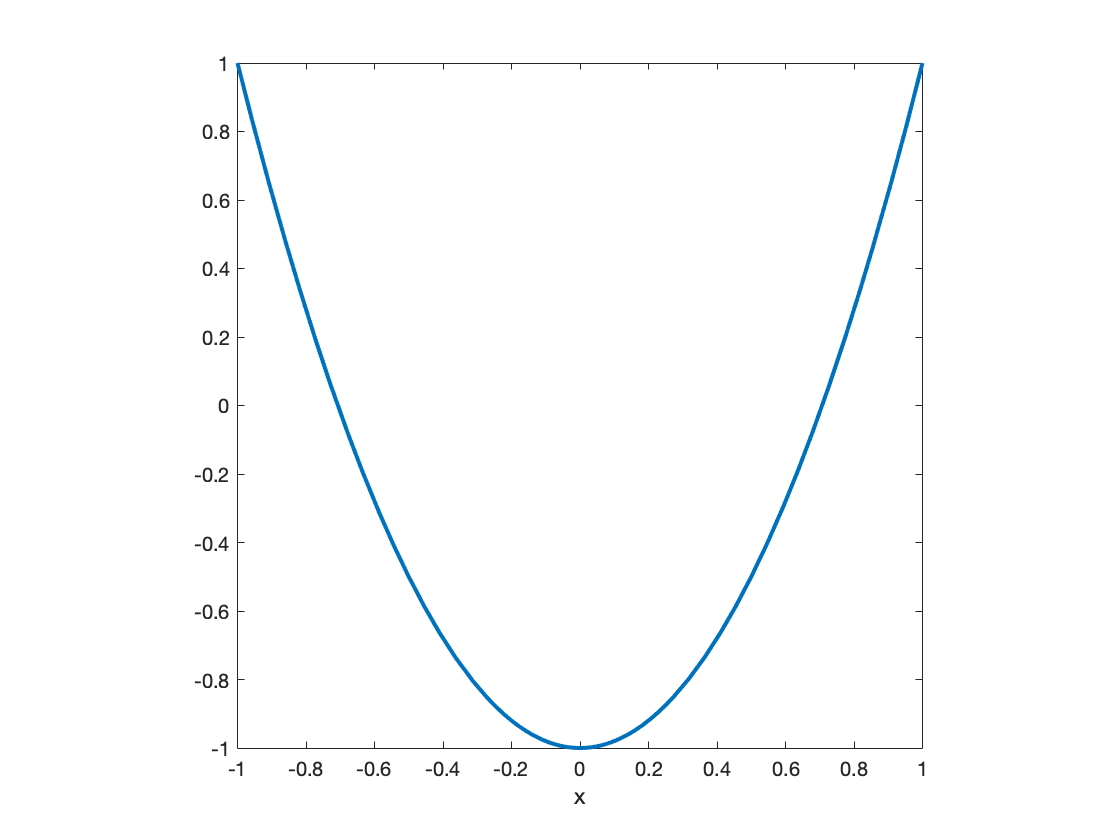
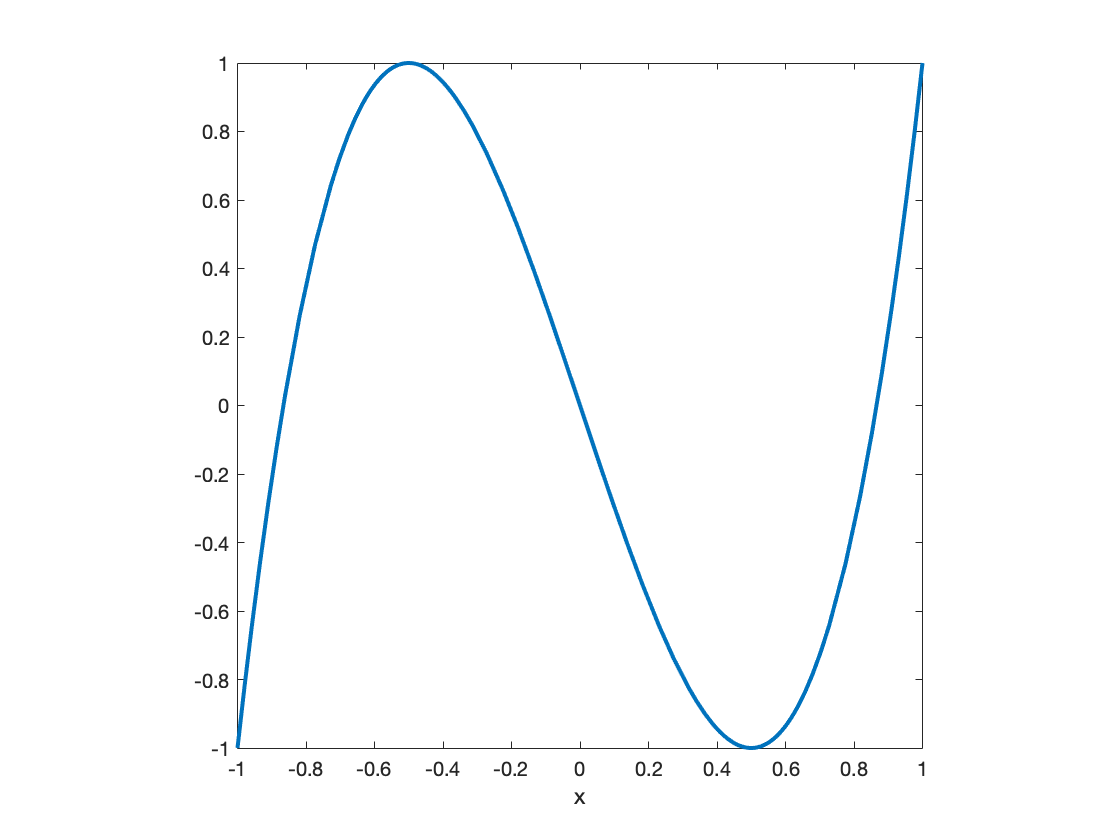
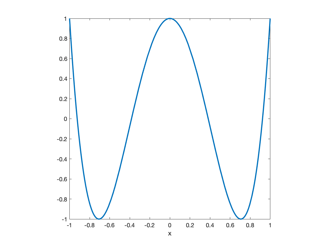
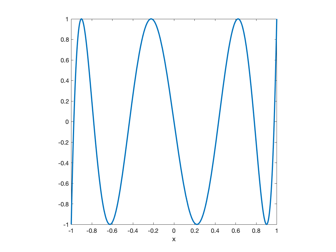
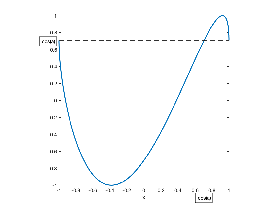
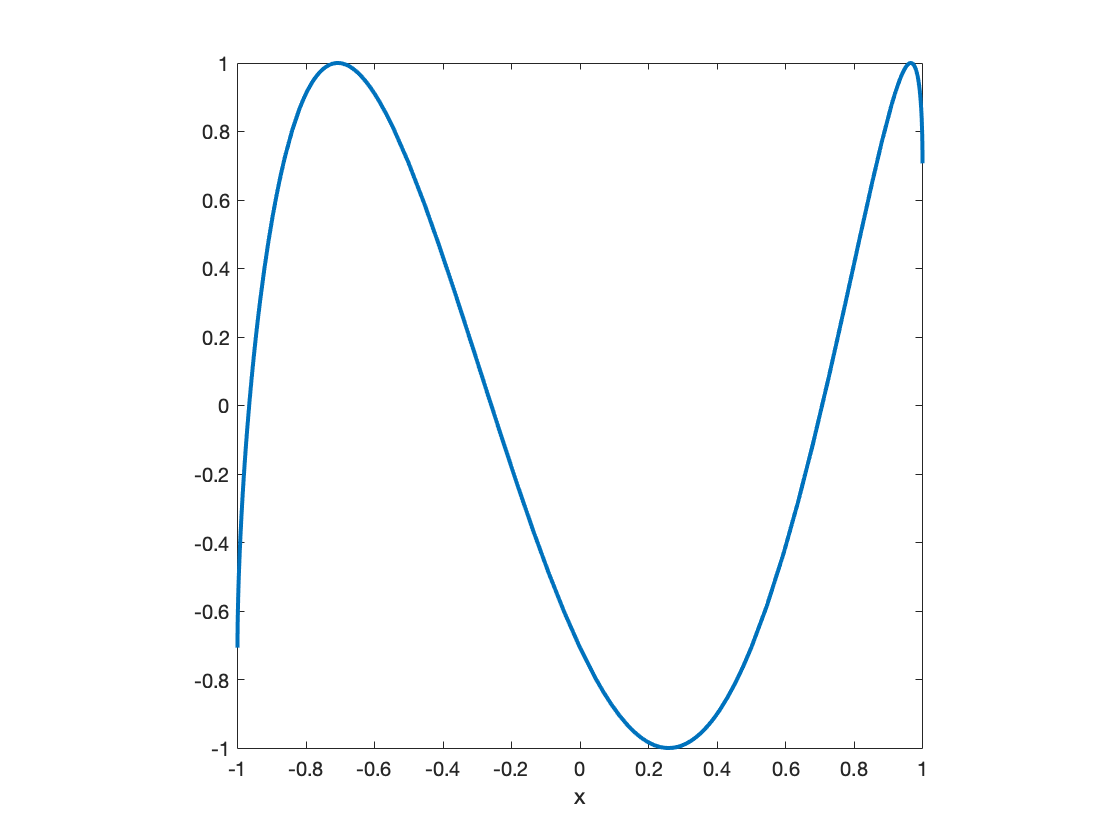
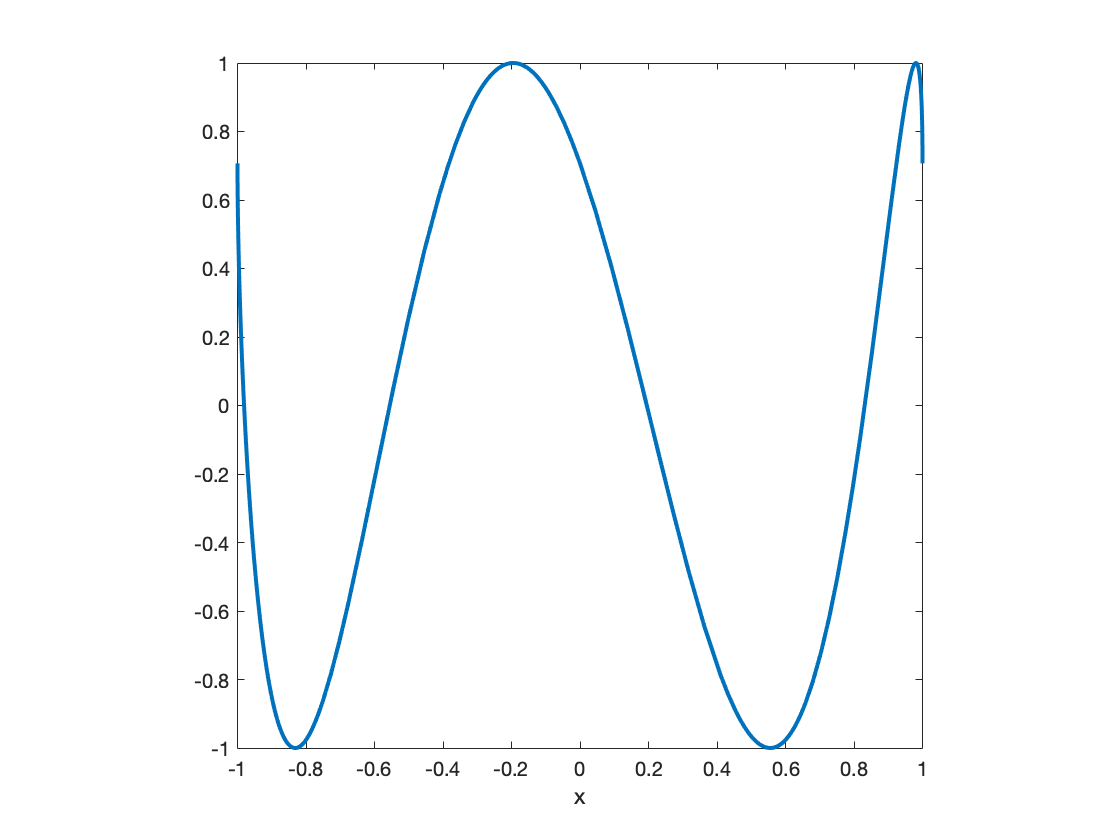
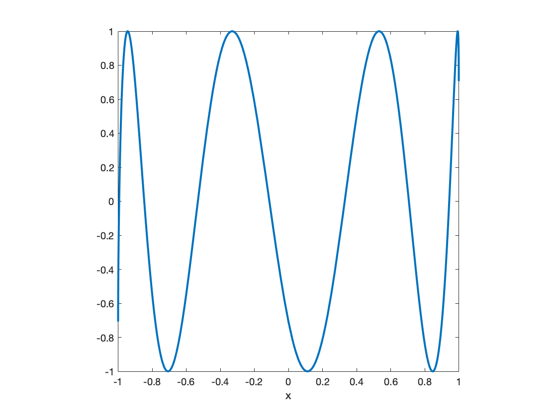
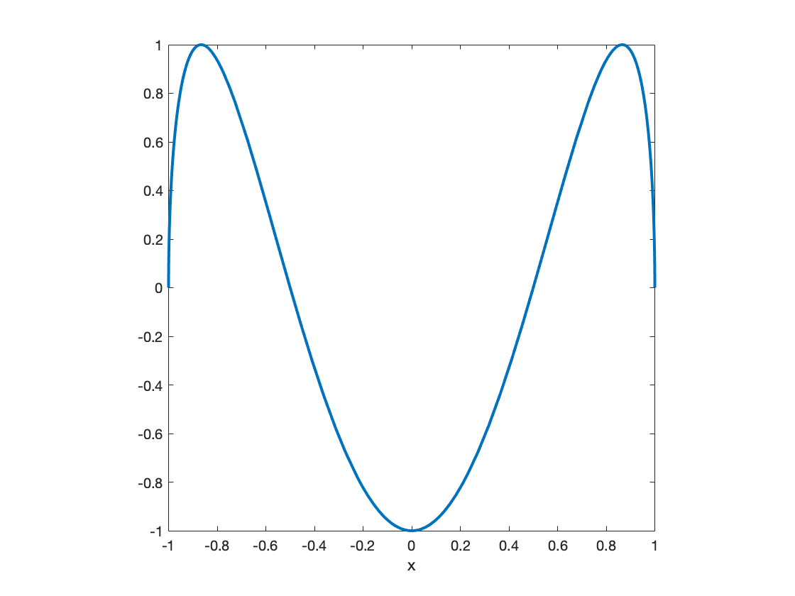
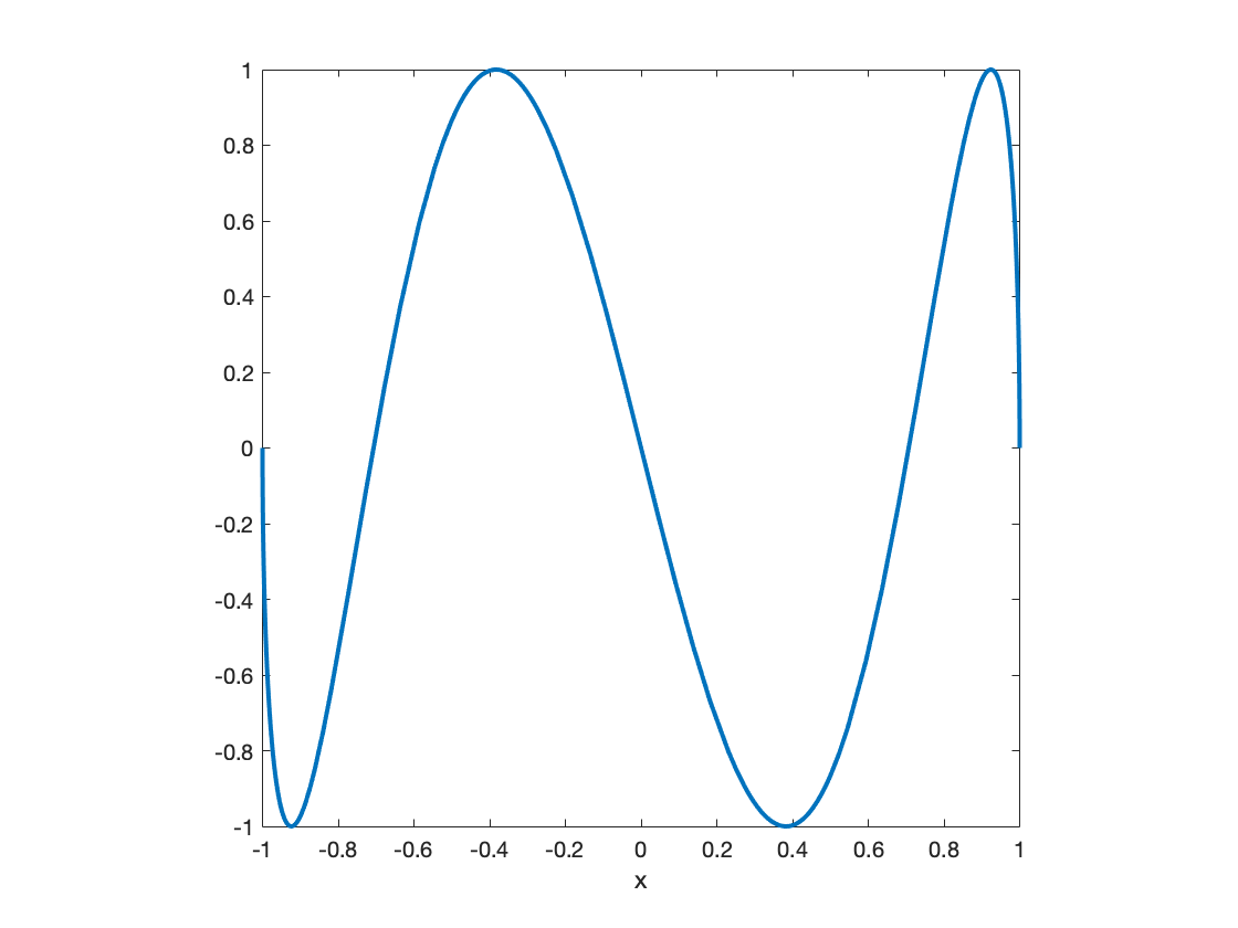
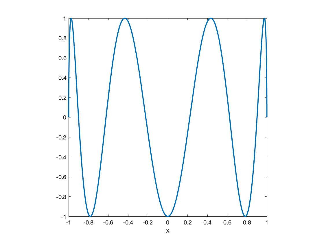
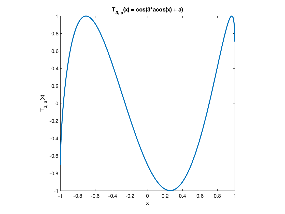
with N=2,3,𝑁23N=2,3,... and a[π2,0]𝑎𝜋20a\in\left[-\frac{\pi}{2},0\right]. TN,asubscript𝑇𝑁𝑎T_{N,a} is called the shifted Chebyshev maps of order N𝑁N. For a=0𝑎0a=0 we have ordinary Chebyshev maps. Some graphs are shown in Fig.1.

Notice that for N=2𝑁2N=2 and a0𝑎0a\neq 0, the map can be decomposed into two independent (ergodic) components, I1=[1,cosa]subscript𝐼11𝑎I_{1}=[-1,\cos a] and I2=[cosa,1]subscript𝐼2𝑎1I_{2}=[\cos a,1], which does not happen for N>2𝑁2N>2, cf. Figs.1e, 1i.

Refer to caption
(a) N=2,a=0formulae-sequence𝑁2𝑎0N=2,a=0
Refer to caption
(b) N=3,a=0formulae-sequence𝑁3𝑎0N=3,a=0
Refer to caption
(c) N=4,a=0formulae-sequence𝑁4𝑎0N=4,a=0
Refer to caption
(d) N=7,a=0formulae-sequence𝑁7𝑎0N=7,a=0
Refer to caption
(e) N=2,a=π/4formulae-sequence𝑁2𝑎𝜋4N=2,a=-\pi/4
Refer to caption
(f) N=3,a=π/4formulae-sequence𝑁3𝑎𝜋4N=3,a=-\pi/4
Refer to caption
(g) N=4,a=π/4formulae-sequence𝑁4𝑎𝜋4N=4,a=-\pi/4
Refer to caption
(h) N=7,a=π/4formulae-sequence𝑁7𝑎𝜋4N=7,a=-\pi/4
Refer to caption
(i) N=2,a=π/2formulae-sequence𝑁2𝑎𝜋2N=2,a=-\pi/2
Refer to caption
(j) N=3,a=π/2formulae-sequence𝑁3𝑎𝜋2N=3,a=-\pi/2
Refer to caption
(k) N=4,a=π/2formulae-sequence𝑁4𝑎𝜋2N=4,a=-\pi/2
Refer to caption
(l) N=7,a=π/2formulae-sequence𝑁7𝑎𝜋2N=7,a=-\pi/2
Figure 1: Graphs of the shifted Chebyshev maps TN,a(x)subscript𝑇𝑁𝑎𝑥T_{N,a}(x), with N𝑁N and a𝑎a indicated in each caption.

2.2 Topological conjugation

Consider a change of variables, x0=cos(πu0)=:cos(u0aN1)x_{0}=\cos(\pi u_{0})=:\cos\left(u_{0}^{\prime}-\frac{a}{N-1}\right), u0(0,1)subscript𝑢001u_{0}\in(0,1), then

xn=cos(Nnπu0+Nn1a+Nn2a++Na+a)=cos(Nnπu0+Nn1N1a)=cos(Nn(πu0+aN1)aN1)=cos(Nnu0aN1).subscript𝑥𝑛superscript𝑁𝑛𝜋subscript𝑢0superscript𝑁𝑛1𝑎superscript𝑁𝑛2𝑎𝑁𝑎𝑎superscript𝑁𝑛𝜋subscript𝑢0superscript𝑁𝑛1𝑁1𝑎superscript𝑁𝑛𝜋subscript𝑢0𝑎𝑁1𝑎𝑁1superscript𝑁𝑛superscriptsubscript𝑢0𝑎𝑁1\begin{split}x_{n}&=\cos\left(N^{n}\pi u_{0}+N^{n-1}a+N^{n-2}a+...+Na+a\right)\\ &=\cos\left(N^{n}\pi u_{0}+\frac{N^{n}-1}{N-1}a\right)\\ &=\cos\left(N^{n}\left(\pi u_{0}+\frac{a}{N-1}\right)-\frac{a}{N-1}\right)\\ &=\cos\left(N^{n}u_{0}^{\prime}-\frac{a}{N-1}\right).\end{split}

So essentially the dynamics can be reduced to a (transformed) N𝑁N-ary shift, at each time step shifting the variable u0:=πu0+aN1=arccos(x0)+aN1assignsuperscriptsubscript𝑢0𝜋subscript𝑢0𝑎𝑁1subscript𝑥0𝑎𝑁1u_{0}^{\prime}:=\pi u_{0}+\frac{a}{N-1}=\arccos(x_{0})+\frac{a}{N-1} by one digit in its N𝑁N-ary representation: un=Nnu0superscriptsubscript𝑢𝑛superscript𝑁𝑛superscriptsubscript𝑢0u_{n}^{\prime}=N^{n}u_{0}^{\prime}, u0(aN1,aN1+π)superscriptsubscript𝑢0𝑎𝑁1𝑎𝑁1𝜋u_{0}^{\prime}\in\left(\frac{a}{N-1},\frac{a}{N-1}+\pi\right).

In fact, it can be shown (see A) that for all N2𝑁subscriptabsent2N\in\mathbb{N}_{\geq 2}, TN,asubscript𝑇𝑁𝑎T_{N,a} is topologically conjugated to a piecewise-linear map gN,asubscript𝑔𝑁𝑎g_{N,a} via the conjugacy h:[1,1][0,1]:1101h:[-1,1]\rightarrow[0,1]

h(x)=1πarccos(x),x[1,1]formulae-sequence𝑥1𝜋arccos𝑥𝑥11h(x)=\frac{1}{\pi}\text{arccos}(-x),\quad x\in[-1,1]

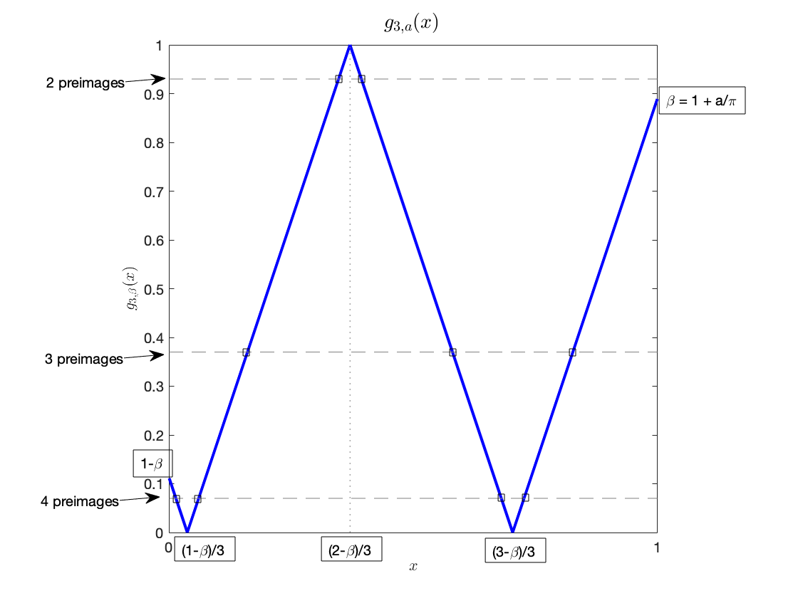
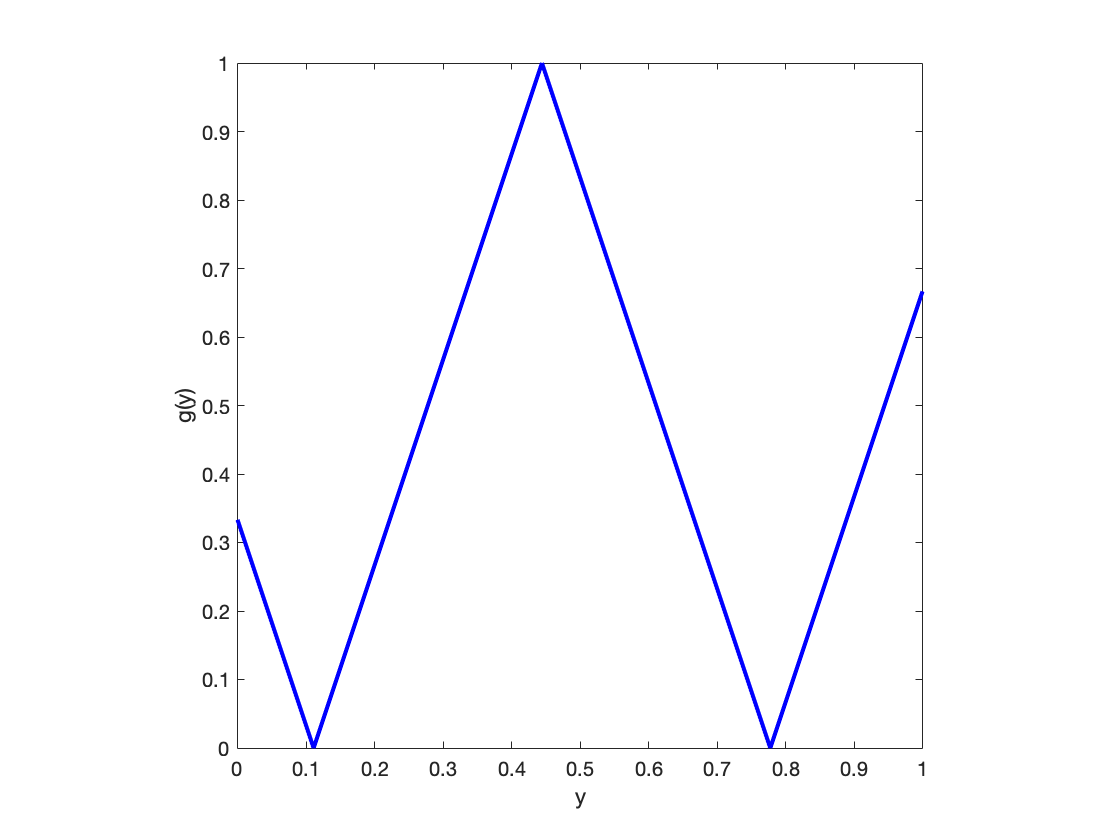
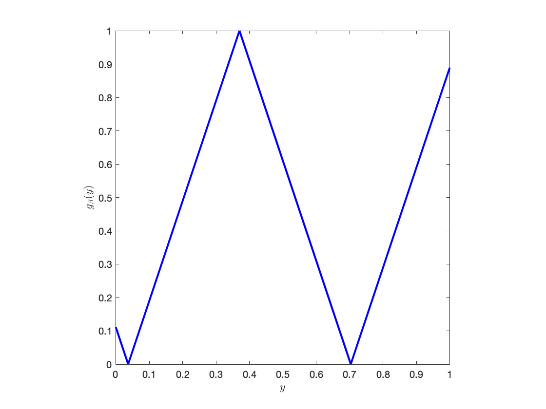
such that hTN,a=gN,ahsubscript𝑇𝑁𝑎subscript𝑔𝑁𝑎h\circ T_{N,a}=g_{N,a}\circ h. The number of branches of gN,asubscript𝑔𝑁𝑎g_{N,a} depends on the order N𝑁N, with the corresponding shifted amount being β:=1+aπassign𝛽1𝑎𝜋\beta:=1+\frac{a}{\pi}. Fig.2 illustrates such a conjugation for N=3𝑁3N=3. One has

g3,a(y)={3y+(1β),y[0,1β3)3y(1β),y[1β3,2β3)3y+(3β),y[2β3,3β3)3y(3β),y[3β3,1].subscript𝑔3𝑎𝑦cases3𝑦1𝛽𝑦01𝛽3otherwise3𝑦1𝛽𝑦1𝛽32𝛽3otherwise3𝑦3𝛽𝑦2𝛽33𝛽3otherwise3𝑦3𝛽𝑦3𝛽31otherwiseg_{3,a}(y)=\begin{cases}-3y+(1-\beta),\quad y\in\left[0,\frac{1-\beta}{3}\right)\\ 3y-(1-\beta),\quad y\in\left[\frac{1-\beta}{3},\frac{2-\beta}{3}\right)\\ -3y+(3-\beta),\quad y\in\left[\frac{2-\beta}{3},\frac{3-\beta}{3}\right)\\ 3y-(3-\beta),\quad y\in\left[\frac{3-\beta}{3},1\right].\end{cases}
Refer to caption
(a) T3,asubscript𝑇3𝑎T_{3,a}
Refer to caption
(b) g3,asubscript𝑔3𝑎g_{3,a}
Figure 2: N=3𝑁3N=3: shifted Chebyshev map TN,asubscript𝑇𝑁𝑎T_{N,a} and its conjugated piecewise-linear map gN,asubscript𝑔𝑁𝑎g_{N,a}.

2.3 Invariant densities

Since the invariant density of a piecewise-linear map is much simpler to find than that of a general shifted Chebyshev map, for a monotonic coordinate transformation we have ρT(x)dx=ρg(y)dysubscript𝜌𝑇𝑥𝑑𝑥subscript𝜌𝑔𝑦𝑑𝑦\rho_{T}(x)dx=\rho_{g}(y)dy, so that the invariant density of TN,asubscript𝑇𝑁𝑎T_{N,a} is given by (we drop the subscripts of T𝑇T and g𝑔g, for simplicity)

ρT(x)=ρgdhdx=1π1x2ρg,x[1,1].formulae-sequencesubscript𝜌𝑇𝑥subscript𝜌𝑔𝑑𝑑𝑥1𝜋1superscript𝑥2subscript𝜌𝑔𝑥11\rho_{T}(x)=\rho_{g}\frac{dh}{dx}=\frac{1}{\pi\sqrt{1-x^{2}}}\rho_{g},\quad x\in[-1,1].

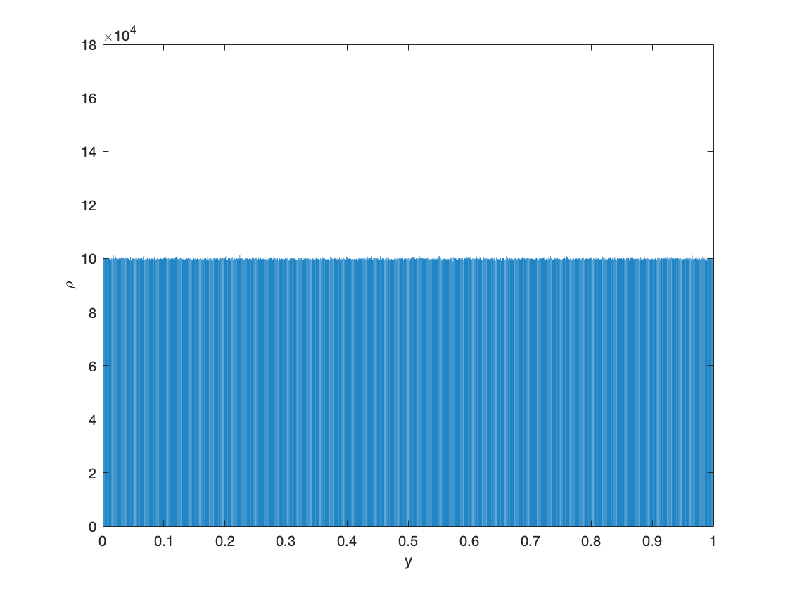
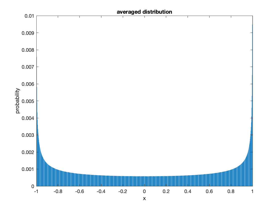
For the simplest case, where a=0𝑎0a=0, TN,0subscript𝑇𝑁0T_{N,0} is the ordinary Chebyshev map, whose conjugated piecewise-linear map is of full-branch111A piecewise linear map is of full-branch if, after a suitable translation along the x𝑥x-axis, each branch is mapped to the whole interval [0,1]01[0,1], making the Lebesgue measure preserved. A counterexample is shown in Fig.2b for which the Lebesgue measure is not invariant. and preserves the Lebesgue measure, ρg=1subscript𝜌𝑔1\rho_{g}=1, so we simply have ρT(x)=1π1x2subscript𝜌𝑇𝑥1𝜋1superscript𝑥2\rho_{T}(x)=\frac{1}{\pi\sqrt{1-x^{2}}}, x[1,1]for-all𝑥11\forall x\in[-1,1]. See the first column in Fig.3.

Furthermore, it can be easily argued that for

even N with all a[π2,0], or odd N with a=0,even N with all a[π2,0], or odd N with a=0\text{even $N$ with all $a\in\left[-\frac{\pi}{2},0\right]$, or odd $N$ with $a=0$}, (\star)

the conjugated piecewise-linear maps are of full-branch so ρg=1subscript𝜌𝑔1\rho_{g}=1 and the invariant density for TN,asubscript𝑇𝑁𝑎T_{N,a} is given by

ρT(x)=1π1x2,x[1,1].formulae-sequencesubscript𝜌𝑇𝑥1𝜋1superscript𝑥2𝑥11\rho_{T}(x)=\frac{1}{\pi\sqrt{1-x^{2}}},\quad x\in[-1,1].

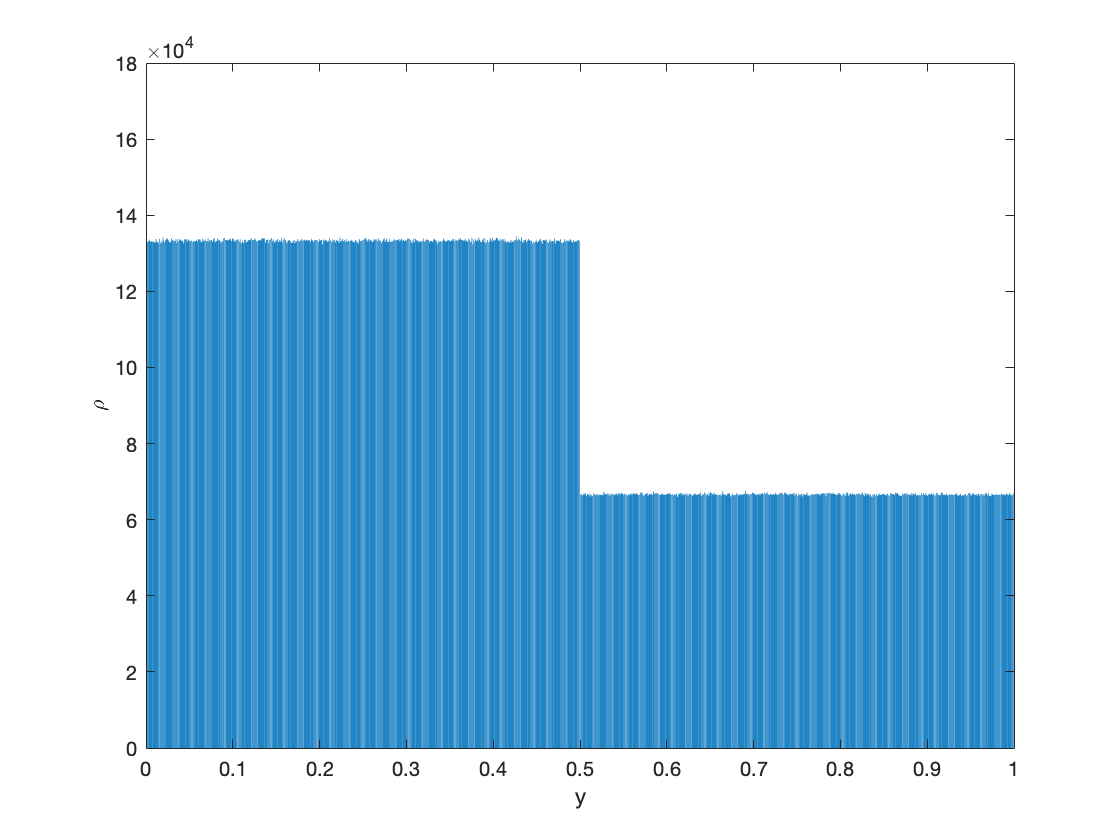
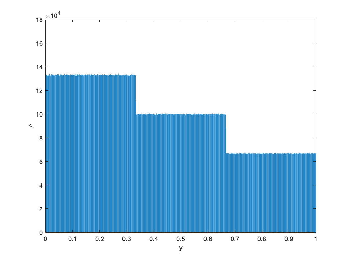
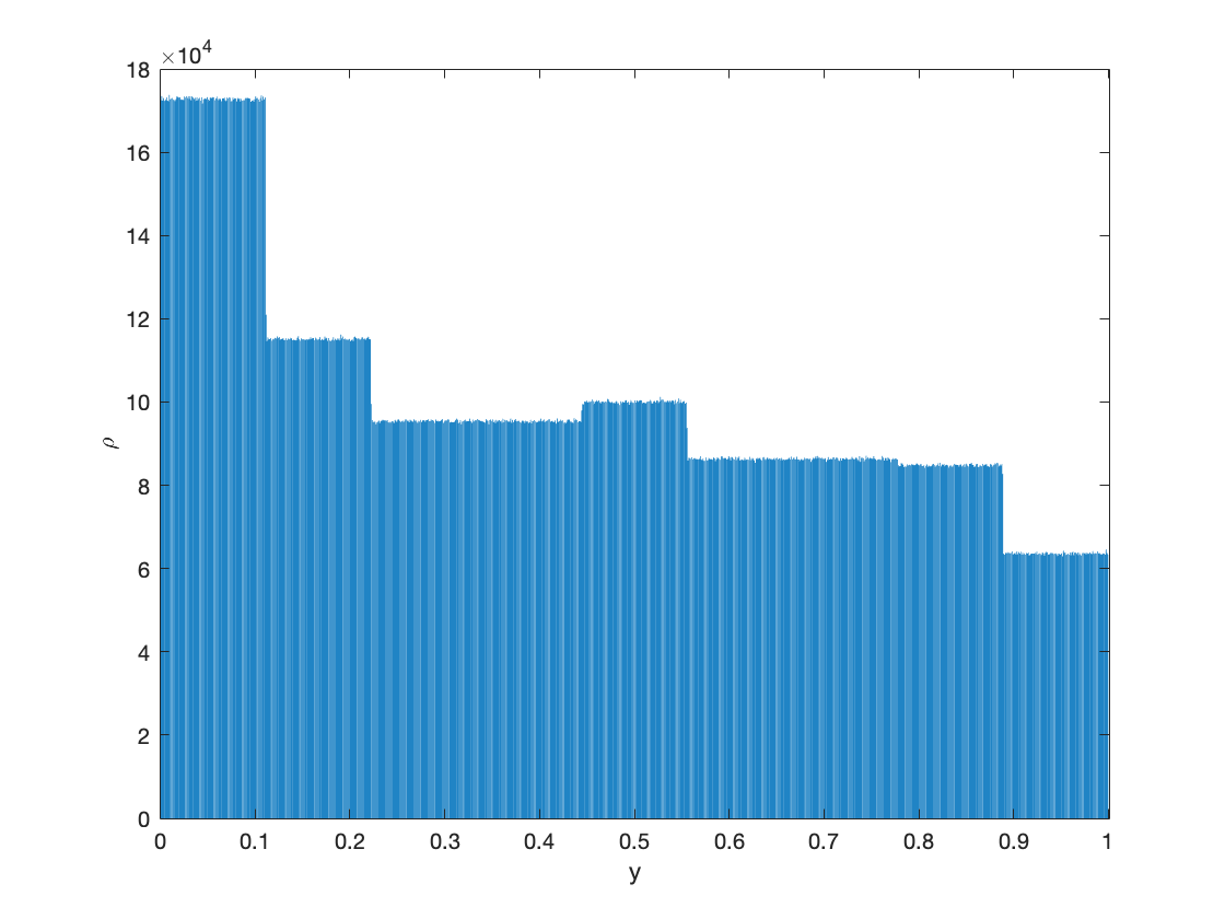
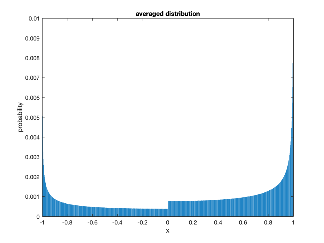
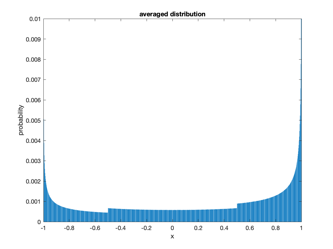
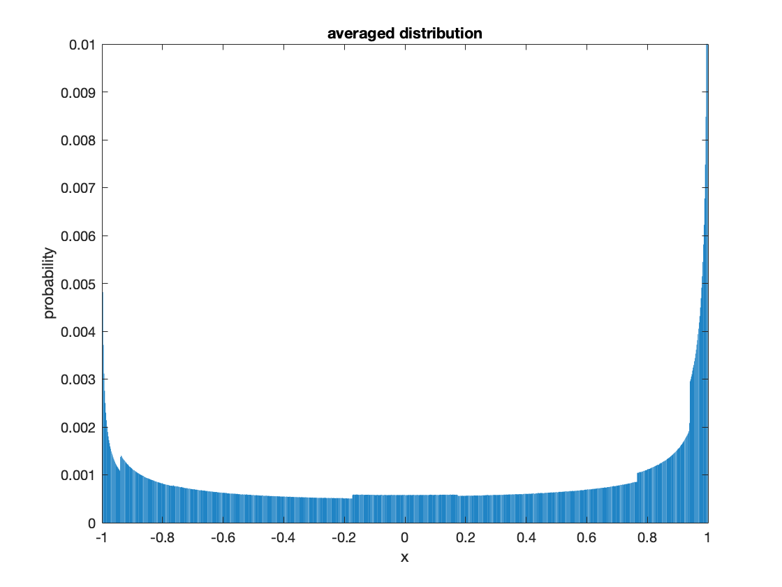
Otherwise, ρgsubscript𝜌𝑔\rho_{g} is a non-trivial stepwise-constant function. Three examples are shown in the second, third and last column in Fig.3. The density in such cases can be calculated by finding the corresponding Markov partition and the transfer matrix, see B for a simple example (N=3,a=π9formulae-sequence𝑁3𝑎𝜋9N=3,a=-\frac{\pi}{9}).

Refer to caption
(a) N=2,a=0formulae-sequence𝑁2𝑎0N=2,a=0
Refer to caption
(b) N=3,a=π/2formulae-sequence𝑁3𝑎𝜋2N=3,a=-\pi/2
Refer to caption
(c) N=3,a=π/3formulae-sequence𝑁3𝑎𝜋3N=3,a=-\pi/3
Refer to caption
(d) N=3,a=π/9formulae-sequence𝑁3𝑎𝜋9N=3,a=-\pi/9
Refer to caption
(e) N=2,a=0formulae-sequence𝑁2𝑎0N=2,a=0
Refer to caption
(f) N=3,a=π/2formulae-sequence𝑁3𝑎𝜋2N=3,a=-\pi/2
Refer to caption
(g) N=3,a=π/3formulae-sequence𝑁3𝑎𝜋3N=3,a=-\pi/3
Refer to caption
(h) N=3,a=π/9formulae-sequence𝑁3𝑎𝜋9N=3,a=-\pi/9
Refer to caption
(i) N=2,a=0formulae-sequence𝑁2𝑎0N=2,a=0
Refer to caption
(j) N=3,a=π/2formulae-sequence𝑁3𝑎𝜋2N=3,a=-\pi/2
Refer to caption
(k) N=3,a=π/3formulae-sequence𝑁3𝑎𝜋3N=3,a=-\pi/3
Refer to caption
(l) N=3,a=π/9formulae-sequence𝑁3𝑎𝜋9N=3,a=-\pi/9
Figure 3: Examples of different invariant densities of TN,asubscript𝑇𝑁𝑎T_{N,a}. First row: graphs of the conjugated piecewise-linear maps gN,asubscript𝑔𝑁𝑎g_{N,a}; second row: their invariant densities ρgsubscript𝜌𝑔\rho_{g}; last row: invariant densities ρTsubscript𝜌𝑇\rho_{T} of the corresponding shifted Chebyshev maps. Values of N𝑁N and a𝑎a are indicated in each caption. Histograms (each with 1,00010001,000 bins) are obtained from simulations: distribution averaged over 10,0001000010,000 trajectories each evolving for 11,0001100011,000(-1,000, to eliminate the initial transient stage) time steps; verified by analytical results.

3 Eigenfunctions of Perron-Frobenius (PF) operator for Chebyshev maps

In this section we describe properties of the eigenfunctions and eigenvalues of the transfer operator for Chebyshev maps, for both the original maps and the shifted ones. These eigenfunctions are important when characterising non-equilibrium properties of the dynamics, i.e. the way how an arbitrary initial density approaches the invariant density. If we write the initial distribution as a linear combination of eigenfunctions, then the time evolution of the density becomes simple, as the application of the (linear) Perron-Frobenius operator just corresponds to multiplying the eigenfunctions in the expansion of the initial density with the corresponding eigenvalues [5, 19].

3.1 Ordinary Chebyshev maps

Recall that the Perron-Frobenius (PF) operator \mathcal{L} for a map describes the time evolution of a set of points characterised by a density function [1, 5, 20, 21]. Eigenfunctions ρ𝜌\rho and the corresponding eigenvalues λ𝜆\lambda satisfy ρ=λρ𝜌𝜆𝜌\mathcal{L}\rho=\lambda\rho, so that the invariant density ρsuperscript𝜌\rho^{*} is the eigenfunction that corresponds to the unit eigenvalue: ρ=ρsuperscript𝜌superscript𝜌\mathcal{L}\rho^{*}=\rho^{*}. For a one-dimensional discrete dynamical system f𝑓f we simply have

ρ(y)=xf1(y)ρ(x)|f(x)|.𝜌𝑦subscript𝑥superscript𝑓1𝑦𝜌𝑥superscript𝑓𝑥\mathcal{L}\rho(y)=\sum_{x\in f^{-1}(y)}\frac{\rho(x)}{|f^{\prime}(x)|}.

It is known [7] that eigenfunctions of the PF operator for the binary shift are given by the Bernoulli polynomials ρ(n)(x)=Bn(x)superscript𝜌𝑛𝑥subscript𝐵𝑛𝑥\rho^{(n)}(x)=B_{n}(x) with eigenvalues λ(n)=2nsuperscript𝜆𝑛superscript2𝑛\lambda^{(n)}=2^{-n}. More generally, eigenfunctions and eigenvalues for an N𝑁N-ary shift are ρ(n)(x)=Bn(x)superscript𝜌𝑛𝑥subscript𝐵𝑛𝑥\rho^{(n)}(x)=B_{n}(x), λ(n)=Nnsuperscript𝜆𝑛superscript𝑁𝑛\lambda^{(n)}=N^{-n} (N2𝑁subscriptabsent2N\in\mathbb{N}_{\geq 2}).

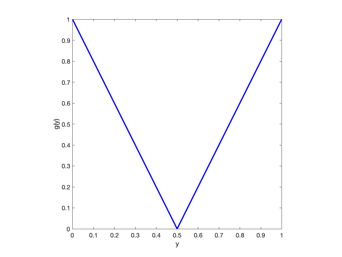
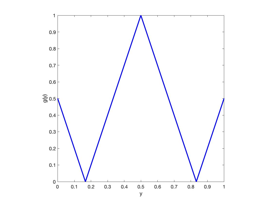
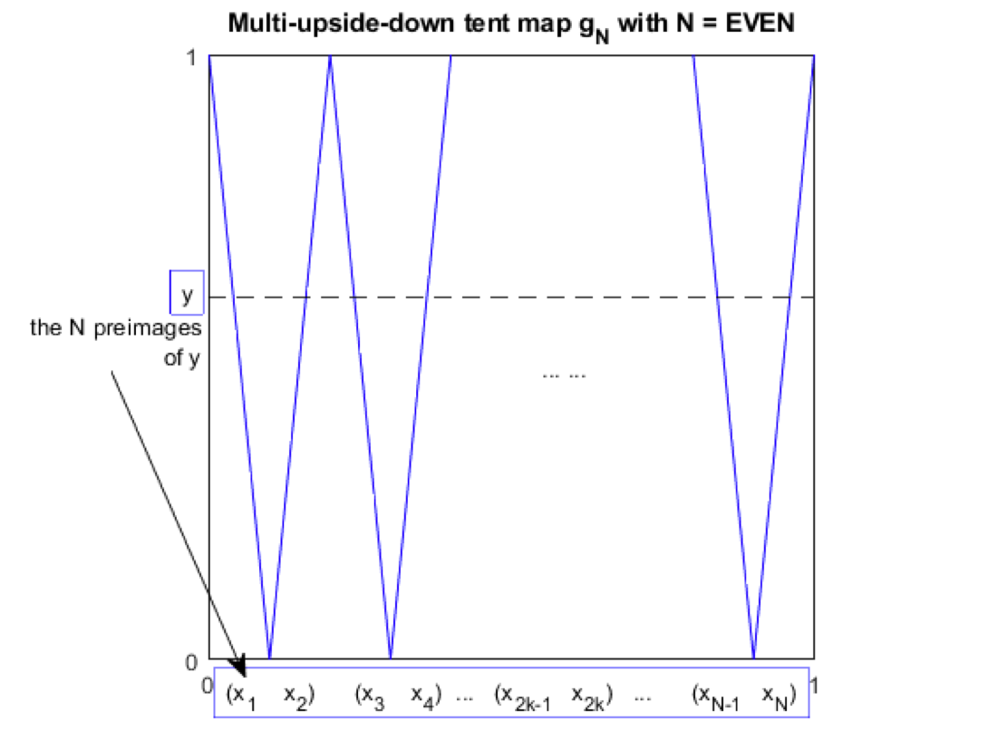
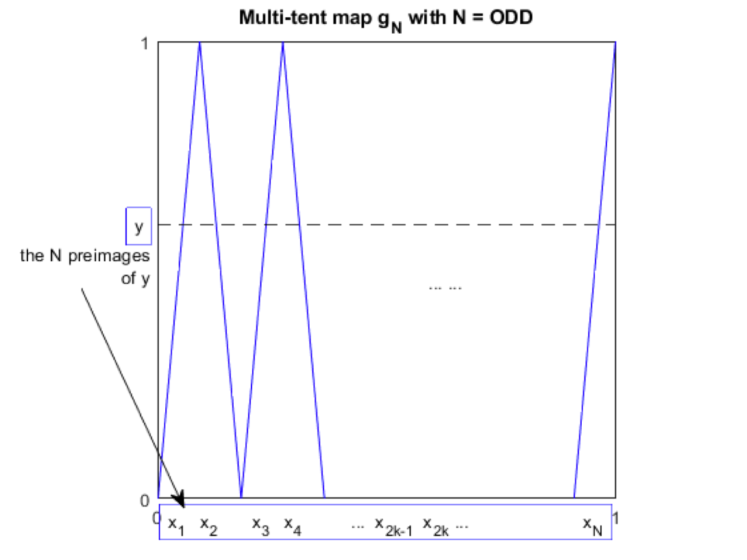
We now use this result to find eigenfunctions for the Chebyshev maps. First consider the ordinary Chebyshev maps TN=TN,0subscript𝑇𝑁subscript𝑇𝑁0T_{N}=T_{N,0}. Via the conjugacy mentioned in the previous section one sees that, for even N=2,4,6,,𝑁246N=2,4,6,..., the piecewise-linear function gNsubscript𝑔𝑁g_{N} consists of a multiple of upside-down tent maps (see Fig.4a), while for odd N=3,5,7,𝑁357N=3,5,7,... the map gNsubscript𝑔𝑁g_{N} consists of a multiple of tent maps (see Fig.4b); let us call them multi-upside-down tent and multi-tent maps, respectively. One can show (details in C), by the Multiplication Theorem and symmetry properties for Bernoulli and Euler polynomials [22], that the eigenfunctions are given by (N2𝑁subscriptabsent2N\in\mathbb{N}_{\geq 2}, n0𝑛subscript0n\in\mathbb{N}_{0})

  • 1.

    for multi-upside-down tents gNsubscript𝑔𝑁g_{N} (even N𝑁N): ρgN(n)(x)=B2n(x2+12)subscriptsuperscript𝜌𝑛subscript𝑔𝑁𝑥subscript𝐵2𝑛𝑥212\rho^{(n)}_{g_{N}}(x)=B_{2n}\left(\frac{x}{2}+\frac{1}{2}\right), with λ(n)=N2nsuperscript𝜆𝑛superscript𝑁2𝑛\lambda^{(n)}=N^{-2n};

  • 2.

    for multi-tents gNsubscript𝑔𝑁g_{N} (odd N𝑁N): ρgN(n,1)(x)=B2n(x)subscriptsuperscript𝜌𝑛1subscript𝑔𝑁𝑥subscript𝐵2𝑛𝑥\rho^{(n,1)}_{g_{N}}(x)=B_{2n}(x), ρgN(n,2)(x)=E2n1(x)subscriptsuperscript𝜌𝑛2subscript𝑔𝑁𝑥subscript𝐸2𝑛1𝑥\rho^{(n,2)}_{g_{N}}(x)=E_{2n-1}(x), with λ(n)=N2nsuperscript𝜆𝑛superscript𝑁2𝑛\lambda^{(n)}=N^{-2n},

where Bnsubscript𝐵𝑛B_{n} and Ensubscript𝐸𝑛E_{n} are Bernoulli and Euler polynomials, defined by their generating functions GB(x,t)=textet1=n=0Bn(x)tnn!subscript𝐺𝐵𝑥𝑡𝑡superscript𝑒𝑥𝑡superscript𝑒𝑡1superscriptsubscript𝑛0subscript𝐵𝑛𝑥superscript𝑡𝑛𝑛G_{B}(x,t)=\frac{te^{xt}}{e^{t}-1}=\sum_{n=0}^{\infty}B_{n}(x)\frac{t^{n}}{n!} and GE(x,t)=2extet+1=n=0En(x)tnn!subscript𝐺𝐸𝑥𝑡2superscript𝑒𝑥𝑡superscript𝑒𝑡1superscriptsubscript𝑛0subscript𝐸𝑛𝑥superscript𝑡𝑛𝑛G_{E}(x,t)=\frac{2e^{xt}}{e^{t}+1}=\sum_{n=0}^{\infty}E_{n}(x)\frac{t^{n}}{n!}, respectively. Notice that the eigenfunctions are independent of the order N𝑁N of the map.

Refer to caption
(a) multi-upside-down tent (for even N𝑁N)
Refer to caption
(b) multi-tent (for odd N𝑁N)
Figure 4: Graphs of piecewise-linear maps to which the ordinary Chebyshev maps conjugated.

By a topological coordinate transformation, ρTN(x)=h(x)ρgN(h(x))subscript𝜌subscript𝑇𝑁𝑥superscript𝑥subscript𝜌subscript𝑔𝑁𝑥\rho_{T_{N}}(x)=h^{\prime}(x)\rho_{g_{N}}(h(x)), where h(x)=1πarccos(x)𝑥1𝜋𝑥h(x)=\frac{1}{\pi}\arccos(-x), we get the following result: the eigenfunctions of the PF operator \mathcal{L} for the ordinary Chebyshev maps TN=TN,0subscript𝑇𝑁subscript𝑇𝑁0T_{N}=T_{N,0} are given by (N2𝑁subscriptabsent2N\in\mathbb{N}_{\geq 2}, n0𝑛subscript0n\in\mathbb{N}_{0})

ρTN(n)(x)=λ(n)ρTN(n)(x)λ(n)=N2n,ρTN(n)(x)={1π1x2B2n(12πarccos(x)+12),if N is even;{ρTN(n,1)=1π1x2B2n(1πarccos(x))ρTN(n,2)=1π1x2E2n1(1πarccos(x)),if N is odd; where Bn(x) and En(x) are Bernoulli and Euler polynomials, respectively.formulae-sequencesuperscriptsubscript𝜌subscript𝑇𝑁𝑛𝑥superscript𝜆𝑛superscriptsubscript𝜌subscript𝑇𝑁𝑛𝑥superscript𝜆𝑛superscript𝑁2𝑛superscriptsubscript𝜌subscript𝑇𝑁𝑛𝑥cases1𝜋1superscript𝑥2subscript𝐵2𝑛12𝜋𝑥12if N is evenotherwisecasessuperscriptsubscript𝜌subscript𝑇𝑁𝑛11𝜋1superscript𝑥2subscript𝐵2𝑛1𝜋𝑥otherwisesuperscriptsubscript𝜌subscript𝑇𝑁𝑛21𝜋1superscript𝑥2subscript𝐸2𝑛11𝜋𝑥otherwiseif N is odd; otherwisewhere Bn(x) and En(x) are Bernoulli and Euler polynomials, respectively.\begin{split}\mathcal{L}\rho_{T_{N}}^{(n)}(x)&=\lambda^{(n)}\rho_{T_{N}}^{(n)}(x)\\ \lambda^{(n)}&=N^{-2n},\\ \rho_{T_{N}}^{(n)}(x)&=\begin{cases}\frac{1}{\pi\sqrt{1-x^{2}}}B_{2n}\left(\frac{1}{2\pi}\arccos(-x)+\frac{1}{2}\right),\quad\text{if $N$ is even};\\ \begin{cases}\rho_{T_{N}}^{(n,1)}=\frac{1}{\pi\sqrt{1-x^{2}}}B_{2n}\left(\frac{1}{\pi}\arccos(-x)\right)\\ \rho_{T_{N}}^{(n,2)}=\frac{1}{\pi\sqrt{1-x^{2}}}E_{2n-1}\left(\frac{1}{\pi}\arccos(-x)\right),\end{cases}\quad\text{if $N$ is odd; }\end{cases}\\ &\text{where $B_{n}(x)$ and $E_{n}(x)$ are Bernoulli and Euler polynomials, respectively.}\end{split} (2)

Note that for odd N𝑁N the eigenfunctions are degenerate, i.e. two independent sets of eigenfunctions exist. One can easily check that when n=0𝑛0n=0 we have λ(0)=1superscript𝜆01\lambda^{(0)}=1 and ρTN(0)=1π1x2subscriptsuperscript𝜌0subscript𝑇𝑁1𝜋1superscript𝑥2\rho^{(0)}_{T_{N}}=\frac{1}{\pi\sqrt{1-x^{2}}}, which is the invariant density of the ordinary Chebyshev maps for all N𝑁N.

It is intriguing that all eigenvalues are real, and the eigenfunctions are orthogonal polynomials. This reminds us of quantum mechanics and the corresponding properties of the eigenfunctions of the Schrödinger operator, although clearly the Perron-Frobenius operator is not a Hermitean operator.

3.2 Shifted Chebyshev maps

First consider maps within the category (\star2.3):

(i) any (even or odd) N𝑁N with a=0𝑎0a=0: These are the ordinary Chebyshev maps, and we have already shown above that eigenfunctions are given by Bernoulli or/and Euler polynomials, with eigenvalues N2nsuperscript𝑁2𝑛N^{-2n};

(ii) even N𝑁N with a[π2,0)𝑎𝜋20a\in\left[-\frac{\pi}{2},0\right): Assume the eigenvalues are the same as in (i), and let N=2q𝑁2𝑞N=2q (q𝑞q\in\mathbb{N}) and consider a=πm𝑎𝜋𝑚a=-\frac{\pi}{m} with m2𝑚subscriptabsent2m\in\mathbb{N}_{\geq 2}. It can be verified that T2q,πmsubscript𝑇2𝑞𝜋𝑚T_{2q,-\frac{\pi}{m}} is topologically semi-conjugated to its corresponding ordinary map T2q,0subscript𝑇2𝑞0T_{2q,0} via the semi-conjugacy function h1(x)=Tm,0(x)subscript1𝑥subscript𝑇𝑚0𝑥h_{1}(x)=-T_{m,0}(x), x[1,1]𝑥11x\in[-1,1] and, moreover,

(Tm,0)T2q,πm=T2q,0(Tm,0)=T2qm,0,subscript𝑇𝑚0subscript𝑇2𝑞𝜋𝑚subscript𝑇2𝑞0subscript𝑇𝑚0subscript𝑇2𝑞𝑚0(-T_{m,0})\circ T_{2q,-\frac{\pi}{m}}=T_{2q,0}\circ(-T_{m,0})=T_{2qm,0}, (3)

i.e. the combined action is equivalent to a single ordinary Chebyshev map (with a multiplicative order N=2qmsuperscript𝑁2𝑞𝑚N^{\prime}=2qm).

From h1(x)=msin(marccosx)1x2superscriptsubscript1𝑥𝑚𝑚𝑥1superscript𝑥2h_{1}^{\prime}(x)=-\frac{m\sin(m\arccos x)}{\sqrt{1-x^{2}}} and eq.(2), also taking into account that there are m𝑚m preimages of the semi-conjugacy h1subscript1h_{1}, we get

ρT2q,πm(n)(x)=|h1(x)|mρT2q,0(n)(h1(x))=1π1x2B2n(m2πarccosx+12).superscriptsubscript𝜌subscript𝑇2𝑞𝜋𝑚𝑛𝑥subscriptsuperscript1𝑥𝑚superscriptsubscript𝜌subscript𝑇2𝑞0𝑛subscript1𝑥1𝜋1superscript𝑥2subscript𝐵2𝑛𝑚2𝜋𝑥12\rho_{T_{2q,-\frac{\pi}{m}}}^{(n)}(x)=\frac{|h^{\prime}_{1}(x)|}{m}\rho_{T_{2q,0}}^{(n)}(h_{1}(x))=\frac{1}{\pi\sqrt{1-x^{2}}}B_{2n}\left(\frac{m}{2\pi}\arccos x+\frac{1}{2}\right).

The situation becomes more complicated for maps outside the category (\star2.3), and we will briefly discuss this case in D. Also, in the case that a𝑎a is not a rational multiple of π𝜋\pi, the form of eigenfunctions is more complicated and in general exhibits some fractal features.

4 Higher-order correlations of shifted Chebyshev maps

4.1 Definition

Generally, the r𝑟rth-order correlation function for a given map xn+1=T(xn)subscript𝑥𝑛1𝑇subscript𝑥𝑛x_{n+1}=T(x_{n}) is defined as

xn1xn2xnr=11ρT(x0)xn1xn2xnr𝑑x0,delimited-⟨⟩subscript𝑥subscript𝑛1subscript𝑥subscript𝑛2subscript𝑥subscript𝑛𝑟superscriptsubscript11subscript𝜌𝑇subscript𝑥0subscript𝑥subscript𝑛1subscript𝑥subscript𝑛2subscript𝑥subscript𝑛𝑟differential-dsubscript𝑥0\langle x_{n_{1}}x_{n_{2}}\cdots x_{n_{r}}\rangle=\int_{-1}^{1}\rho_{T}(x_{0})x_{n_{1}}x_{n_{2}}\cdots x_{n_{r}}dx_{0},

where the average is taken over all initial points weighted with respect to the invariant density ρTsubscript𝜌𝑇\rho_{T}. In the case of shifted Chebyshev maps T𝑇T in category (\star2.3), we obtain after some calculation

xn1xnr=2rσ[exp(ial=1rσlNnl1N1)δ(l=1rσlNnl,0)],delimited-⟨⟩subscript𝑥subscript𝑛1subscript𝑥subscript𝑛𝑟superscript2𝑟subscript𝜎delimited-[]𝑖𝑎superscriptsubscript𝑙1𝑟subscript𝜎𝑙superscript𝑁subscript𝑛𝑙1𝑁1𝛿superscriptsubscript𝑙1𝑟subscript𝜎𝑙superscript𝑁subscript𝑛𝑙0\langle x_{n_{1}}\cdots x_{n_{r}}\rangle=2^{-r}\sum_{\sigma}\left[\exp\left(ia\sum_{l=1}^{r}\sigma_{l}\frac{N^{n_{l}}-1}{N-1}\right)\cdot\delta\left(\sum_{l=1}^{r}\sigma_{l}N^{n_{l}},0\right)\right], (4)

where the sum over σ𝜎\sigma is a summation over all possible spin configurations σ:=(σ1,σ2,,σr)assign𝜎subscript𝜎1subscript𝜎2subscript𝜎𝑟\sigma:=(\sigma_{1},\sigma_{2},...,\sigma_{r}), σl{1,+1}subscript𝜎𝑙11\sigma_{l}\in\{-1,+1\}, and δ(x,0)𝛿𝑥0\delta(x,0) is the Kronecker delta defined as being 1 if x=0𝑥0x=0 and 0 else. Details in E.

4.2 Ordinary Chebyshev maps

In this case

TN,0(x)=cos(Narccosx),x[1,1]formulae-sequencesubscript𝑇𝑁0𝑥𝑁arccos𝑥𝑥11T_{N,0}(x)=\cos(N\text{arccos}x),\quad x\in[-1,1]

which can be written as polynomials:

T2,0(x)=2x21T3,0(x)=4x33xT4,0(x)=8x48x2+1T5,0(x)=16x520x3+5xsubscript𝑇20𝑥2superscript𝑥21subscript𝑇30𝑥4superscript𝑥33𝑥subscript𝑇40𝑥8superscript𝑥48superscript𝑥21subscript𝑇50𝑥16superscript𝑥520superscript𝑥35𝑥\begin{split}T_{2,0}(x)&=2x^{2}-1\\ T_{3,0}(x)&=4x^{3}-3x\\ T_{4,0}(x)&=8x^{4}-8x^{2}+1\\ T_{5,0}(x)&=16x^{5}-20x^{3}+5x\\ \vdots\end{split}

The correlation functions reduce to

xn1xn2xnra=0=12rσδ(l=1rσlNnl,0).subscriptdelimited-⟨⟩subscript𝑥subscript𝑛1subscript𝑥subscript𝑛2subscript𝑥subscript𝑛𝑟𝑎01superscript2𝑟subscript𝜎𝛿superscriptsubscript𝑙1𝑟subscript𝜎𝑙superscript𝑁subscript𝑛𝑙0\langle x_{n_{1}}x_{n_{2}}\cdots x_{n_{r}}\rangle_{a=0}=\frac{1}{2^{r}}\sum_{\sigma}\delta\left(\sum_{l=1}^{r}\sigma_{l}N^{n_{l}},0\right). (5)

The non-vanishing correlations of TN,0subscript𝑇𝑁0T_{N,0} correspond to tuples (n1,,nr)subscript𝑛1subscript𝑛𝑟(n_{1},...,n_{r}) that solve the diophantine equations

l=1rσlNnl=0superscriptsubscript𝑙1𝑟subscript𝜎𝑙superscript𝑁subscript𝑛𝑙0\sum_{l=1}^{r}\sigma_{l}N^{n_{l}}=0 (6)

for σl{1,+1}subscript𝜎𝑙11\sigma_{l}\in\{-1,+1\}. For a given N𝑁N, for each r=2,3,𝑟23r=2,3,..., the tuples that solve the above equations can be represented by simple graphs (N𝑁N-ary double forests), and this graph-theoretical method was introduced in [2, 3]. It turns out that for all odd N𝑁N with odd r𝑟r, the correlation for TN,0subscript𝑇𝑁0T_{N,0} vanishes identically.

4.3 Distinctive property of higher-order correlations for Chebyshev maps

We now come to the central result of this paper, namely the fact that Chebyshev maps are distinguished as having a minimum set of higher-order correlations. First, let us discuss why higher-order correlation functions are relevant, and why, for example, the 2-point correlation is not sufficient.

Consider a variable defined by a sum of iterates of a given map T𝑇T, yn:=j=1nxjassignsubscript𝑦𝑛superscriptsubscript𝑗1𝑛subscript𝑥𝑗y_{n}:=\sum_{j=1}^{n}x_{j}, xj=T(xj1)subscript𝑥𝑗𝑇subscript𝑥𝑗1x_{j}=T(x_{j-1}); the r𝑟rth moment is then given by

ynr=j1=1njr=1nxj1xjr=j1=1njr=1nxj1xjr.delimited-⟨⟩superscriptsubscript𝑦𝑛𝑟delimited-⟨⟩superscriptsubscriptsubscript𝑗11𝑛superscriptsubscriptsubscript𝑗𝑟1𝑛subscript𝑥subscript𝑗1subscript𝑥subscript𝑗𝑟superscriptsubscriptsubscript𝑗11𝑛superscriptsubscriptsubscript𝑗𝑟1𝑛delimited-⟨⟩subscript𝑥subscript𝑗1subscript𝑥subscript𝑗𝑟\langle y_{n}^{r}\rangle=\langle\sum_{j_{1}=1}^{n}\cdots\sum_{j_{r}=1}^{n}x_{j_{1}}\cdots x_{j_{r}}\rangle=\sum_{j_{1}=1}^{n}\cdots\sum_{j_{r}=1}^{n}\langle x_{j_{1}}\cdots x_{j_{r}}\rangle.

These types of sums are motivated by deterministic diffusion processes and generalised versions of Central limit theorems [16, 23, 24, 25].

If we know all the higher-order correlation functions of T𝑇T, we will have the knowledge of all moments of ynsubscript𝑦𝑛y_{n}. For any smooth observable defined by a function f𝑓f of the variable ynsubscript𝑦𝑛y_{n}, we can write down its Taylor expansion as f(yn)=jbjynj𝑓subscript𝑦𝑛subscript𝑗subscript𝑏𝑗superscriptsubscript𝑦𝑛𝑗f(y_{n})=\sum_{j}b_{j}y_{n}^{j}; its average is therefore given by

f(yn)=jbjynj.delimited-⟨⟩𝑓subscript𝑦𝑛subscript𝑗subscript𝑏𝑗delimited-⟨⟩superscriptsubscript𝑦𝑛𝑗\langle f(y_{n})\rangle=\sum_{j}b_{j}\langle y_{n}^{j}\rangle.

Hence, provided all the moments of ynsubscript𝑦𝑛y_{n} (and thus higher-order correlations of xnsubscript𝑥𝑛x_{n}) are known, we can calculate the expectation of this arbitrary observable.

Now, consider an arbitrary map W𝑊W that is conjugated to an N𝑁N-ary shift. Assume that the iterates wnsubscript𝑤𝑛w_{n} of W𝑊W can be written as

wn=f(Nnu)subscript𝑤𝑛𝑓superscript𝑁𝑛𝑢w_{n}=f(N^{n}u)

with w0=f(u)subscript𝑤0𝑓𝑢w_{0}=f(u), where f𝑓f is some smooth periodic function (for Chebyshev maps this is simply f(u)=cosπu𝑓𝑢𝜋𝑢f(u)=\cos\pi u), indicating that it is conjugated to an N𝑁N-ary shift dynamics. If f𝑓f has the Fourier representation

f(u)=k=akeiπku,𝑓𝑢superscriptsubscript𝑘subscript𝑎𝑘superscript𝑒𝑖𝜋𝑘𝑢f(u)=\sum_{k=-\infty}^{\infty}a_{k}e^{i\pi ku},

then the r𝑟rth-order correlation of iterates of W𝑊W evaluates to

wn1wn2wnr=k1=k2=kr=ak1ak2akrδ(k1Nn1+k2Nn2++krNnr,0),delimited-⟨⟩subscript𝑤subscript𝑛1subscript𝑤subscript𝑛2subscript𝑤subscript𝑛𝑟superscriptsubscriptsubscript𝑘1superscriptsubscriptsubscript𝑘2superscriptsubscriptsubscript𝑘𝑟subscript𝑎subscript𝑘1subscript𝑎subscript𝑘2subscript𝑎subscript𝑘𝑟𝛿subscript𝑘1superscript𝑁subscript𝑛1subscript𝑘2superscript𝑁subscript𝑛2subscript𝑘𝑟superscript𝑁subscript𝑛𝑟0\langle w_{n_{1}}w_{n_{2}}\cdots w_{n_{r}}\rangle=\sum_{k_{1}=-\infty}^{\infty}\sum_{k_{2}=-\infty}^{\infty}\cdots\sum_{k_{r}=-\infty}^{\infty}a_{k_{1}}a_{k_{2}}\cdots a_{k_{r}}\delta(k_{1}N^{n_{1}}+k_{2}N^{n_{2}}+\cdots+k_{r}N^{n_{r}},0),

by a simple generalisation of the derivation that we presented in E. Non-zero correlations occur if a given tuple (n1,n2,,nr)subscript𝑛1subscript𝑛2subscript𝑛𝑟(n_{1},n_{2},...,n_{r}) solves any of the diophantine equations

j=1rkjNnj=0,kj.formulae-sequencesuperscriptsubscript𝑗1𝑟subscript𝑘𝑗superscript𝑁subscript𝑛𝑗0subscript𝑘𝑗\sum_{j=1}^{r}k_{j}N^{n_{j}}=0,\quad k_{j}\in\mathbb{Z}.

These equations in general have much more solutions than those for Chebyshev maps, as in the latter case each coefficient only takes one of the two integer values kj{1,+1}subscript𝑘𝑗11k_{j}\in\{-1,+1\}, whereas in this more general case the kjsubscript𝑘𝑗k_{j} can take on any integer values. If we regard the original Chebyshev correlations as being described by an Ising model (up-down spin configurations), then this would be a generalisation towards a Potts model (integer spin configurations) [5].

The number of tuples (n1,,nr)subscript𝑛1subscript𝑛𝑟(n_{1},\ldots,n_{r}) with non-zero correlations is minimised when the underlying map is from the Chebyshev family, in which case only the coefficients a±1subscript𝑎plus-or-minus1a_{\pm 1} are non-zero (a1=a1=12subscript𝑎1subscript𝑎112a_{-1}=a_{1}=\frac{1}{2}) in the Fourier representation of the conjugating function f(u)=cosπu=12(eiπu+eiπu)=a1eiπu+a1eiπu𝑓𝑢𝜋𝑢12superscript𝑒𝑖𝜋𝑢superscript𝑒𝑖𝜋𝑢subscript𝑎1superscript𝑒𝑖𝜋𝑢subscript𝑎1superscript𝑒𝑖𝜋𝑢f(u)=\cos\pi u=\frac{1}{2}(e^{-i\pi u}+e^{i\pi u})=a_{-1}e^{-i\pi u}+a_{1}e^{i\pi u}. Hence, Chebyshev maps can be regarded as producing a “minimum skeleton” of higher-order correlations. They can serve as the most random-like deterministic system in this context, in the sense of a minimum set of correlations, or strongest possible similarity to white noise for a smooth deterministic dynamics.

4.4 Example: two-point correlations

Our result of the previous subsection implies that the higher-order correlation functions for (ordinary) Chebyshev maps are identically equal to 0 for more tuples (n1,,nr)subscript𝑛1subscript𝑛𝑟(n_{1},\ldots,n_{r}) than those for other N𝑁N-ary shift systems, indicating that, although they are equally chaotic in the sense of topology (i.e., topologically conjugated to each other), one appears more random than the other in the sense of vanishing correlations. Let us now consider the special case r=2𝑟2r=2. It is known (see F) that the two-point correlation function for the binary shift map (normalised, i.e., with average 1212\frac{1}{2} subtracted) is given by

wn1wn2binary=112(12)|n1n2|,subscriptdelimited-⟨⟩subscript𝑤subscript𝑛1subscript𝑤subscript𝑛2binary112superscript12subscript𝑛1subscript𝑛2\langle w_{n_{1}}w_{n_{2}}\rangle_{\text{binary}}=\frac{1}{12}\cdot\left(\frac{1}{2}\right)^{|n_{1}-n_{2}|},

while for the 222nd-order ordinary Chebyshev map T2,0subscript𝑇20T_{2,0} it vanishes immediately, as there is no solution to the corresponding diophantine equations, i.e. xn1xn2T2,0=12δn1,n2subscriptdelimited-⟨⟩subscript𝑥subscript𝑛1subscript𝑥subscript𝑛2subscript𝑇2012subscript𝛿subscript𝑛1subscript𝑛2\langle x_{n_{1}}x_{n_{2}}\rangle_{T_{2,0}}=\frac{1}{2}\delta_{n_{1},n_{2}}.

The two-point correlation function for a general N𝑁N-ary shift (normalised) can be shown (F) to be

wn1wn2Nary=16N(1N)|n1n2|.subscriptdelimited-⟨⟩subscript𝑤subscript𝑛1subscript𝑤subscript𝑛2𝑁ary16𝑁superscript1𝑁subscript𝑛1subscript𝑛2\langle w_{n_{1}}w_{n_{2}}\rangle_{N-\text{ary}}=\frac{1}{6N}\cdot\left(\frac{1}{N}\right)^{|n_{1}-n_{2}|}.

Comparing with the two-point correlation function for the N𝑁Nth-order ordinary Chebyshev map TN,0subscript𝑇𝑁0T_{N,0}, for which

xn1xn2TN,0=12δn1,n2,N2,formulae-sequencesubscriptdelimited-⟨⟩subscript𝑥subscript𝑛1subscript𝑥subscript𝑛2subscript𝑇𝑁012subscript𝛿subscript𝑛1subscript𝑛2for-all𝑁2\langle x_{n_{1}}x_{n_{2}}\rangle_{T_{N,0}}=\frac{1}{2}\delta_{n_{1},n_{2}},\quad\forall N\geq 2,

we see that for N𝑁N-ary shifts it decreases exponentially in N𝑁N but it never vanishes identically, while for the Chebyshev maps the two-point correlation does not depend on N𝑁N and it attains zero whenever n1n2subscript𝑛1subscript𝑛2n_{1}\neq n_{2}.

For shifted Chebyshev maps TN,asubscript𝑇𝑁𝑎T_{N,a} in the category (\star2.3), we can write down the two-point correlation functions explicitly (assuming stationarity)

xnxn+kTN,a=x0xkTN,a=11ρ(x0)x0TN,a(k)(x0)𝑑x0=111π1cos2(u0aN1)cos(u0aN1)cos(Nku0aN1)d[cos(u0aN1)]=12[sin(2aN1Nkπ)+sin(2aN1)Nk+1sin(Nkπ)Nk1].subscriptdelimited-⟨⟩subscript𝑥𝑛subscript𝑥𝑛𝑘subscript𝑇𝑁𝑎subscriptdelimited-⟨⟩subscript𝑥0subscript𝑥𝑘subscript𝑇𝑁𝑎superscriptsubscript11𝜌subscript𝑥0subscript𝑥0superscriptsubscript𝑇𝑁𝑎𝑘subscript𝑥0differential-dsubscript𝑥0superscriptsubscript111𝜋1superscript2superscriptsubscript𝑢0𝑎𝑁1superscriptsubscript𝑢0𝑎𝑁1superscript𝑁𝑘superscriptsubscript𝑢0𝑎𝑁1𝑑delimited-[]superscriptsubscript𝑢0𝑎𝑁112delimited-[]2𝑎𝑁1superscript𝑁𝑘𝜋2𝑎𝑁1superscript𝑁𝑘1superscript𝑁𝑘𝜋superscript𝑁𝑘1\begin{split}&\langle x_{n}x_{n+k}\rangle_{T_{N,a}}\\ =&\langle x_{0}x_{k}\rangle_{T_{N,a}}\\ =&\int_{-1}^{1}\rho(x_{0})x_{0}T_{N,a}^{(k)}(x_{0})dx_{0}\\ =&\int_{-1}^{1}\frac{1}{\pi\sqrt{1-\cos^{2}\left(u_{0}^{\prime}-\frac{a}{N-1}\right)}}\cos\left(u_{0}^{\prime}-\frac{a}{N-1}\right)\cos\left(N^{k}u_{0}^{\prime}-\frac{a}{N-1}\right)d\left[\cos\left(u_{0}^{\prime}-\frac{a}{N-1}\right)\right]\\ =&\frac{1}{2}\left[\frac{\sin\left(\frac{2a}{N-1}-N^{k}\pi\right)+\sin\left(\frac{2a}{N-1}\right)}{N^{k}+1}-\frac{\sin\left(N^{k}\pi\right)}{N^{k}-1}\right].\end{split}

One can check that for

i) a=0𝑎0a=0, the ordinary Chebyshev maps, we have identically vanishing correlation for all k0𝑘0k\neq 0; otherwise we have the second moment x02TN,0=11ρ(x)x2𝑑x=11x2π1x2𝑑x=12subscriptdelimited-⟨⟩superscriptsubscript𝑥02subscript𝑇𝑁0superscriptsubscript11𝜌𝑥superscript𝑥2differential-d𝑥superscriptsubscript11superscript𝑥2𝜋1superscript𝑥2differential-d𝑥12\langle x_{0}^{2}\rangle_{T_{N,0}}=\int_{-1}^{1}\rho(x)x^{2}dx=\int_{-1}^{1}\frac{x^{2}}{\pi\sqrt{1-x^{2}}}dx=\frac{1}{2}.

ii) a=π2𝑎𝜋2a=-\frac{\pi}{2}, we have, for k=0𝑘0k=0

x02TN,π/2=0πcos2(uaN1)𝑑u=π2,subscriptdelimited-⟨⟩superscriptsubscript𝑥02subscript𝑇𝑁𝜋2superscriptsubscript0𝜋superscript2𝑢𝑎𝑁1differential-d𝑢𝜋2\langle x_{0}^{2}\rangle_{T_{N,-\pi/2}}=\int_{0}^{\pi}\cos^{2}\left(u-\frac{a}{N-1}\right)du=\frac{\pi}{2},

and for k>0𝑘0k>0

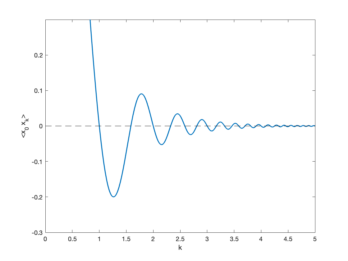
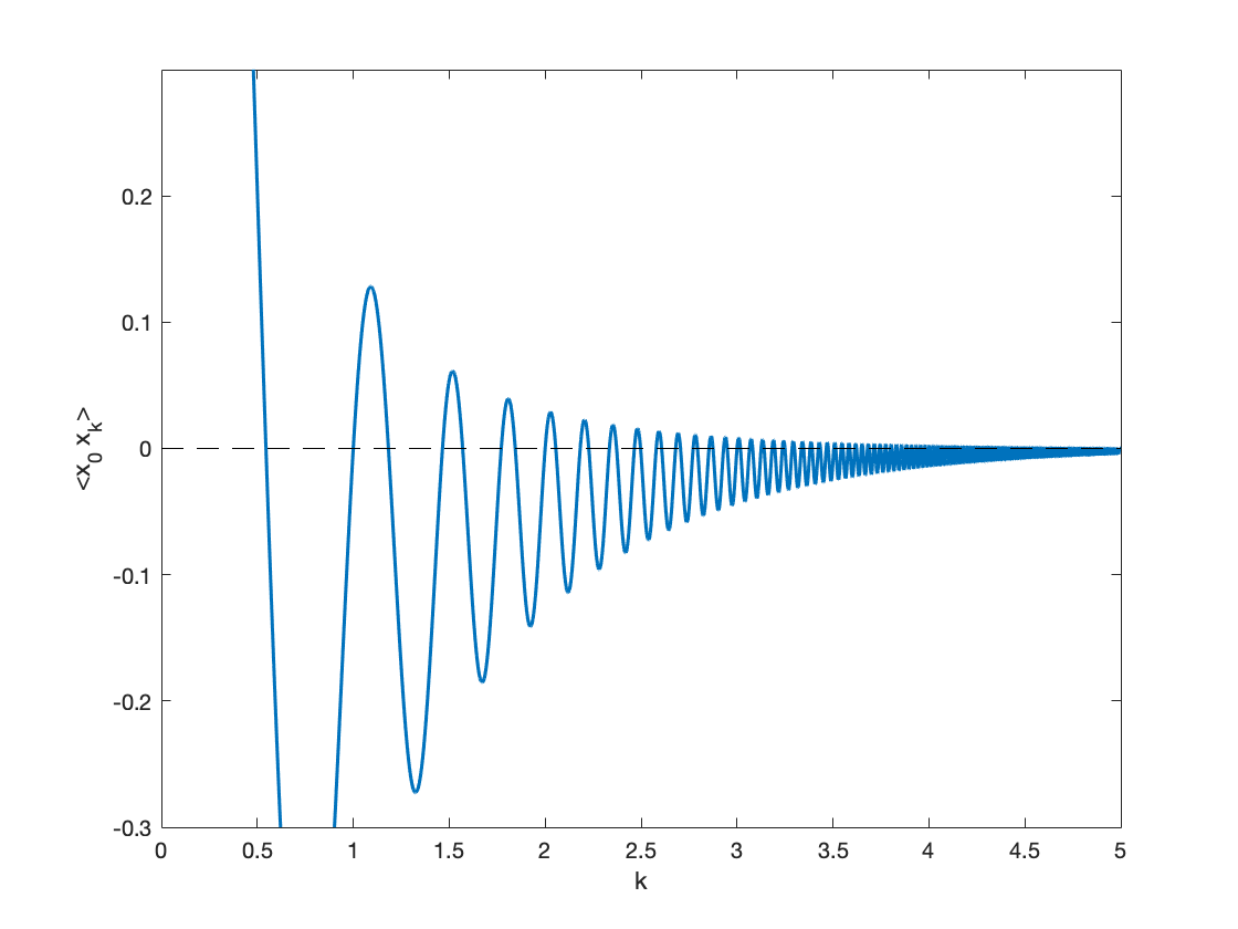
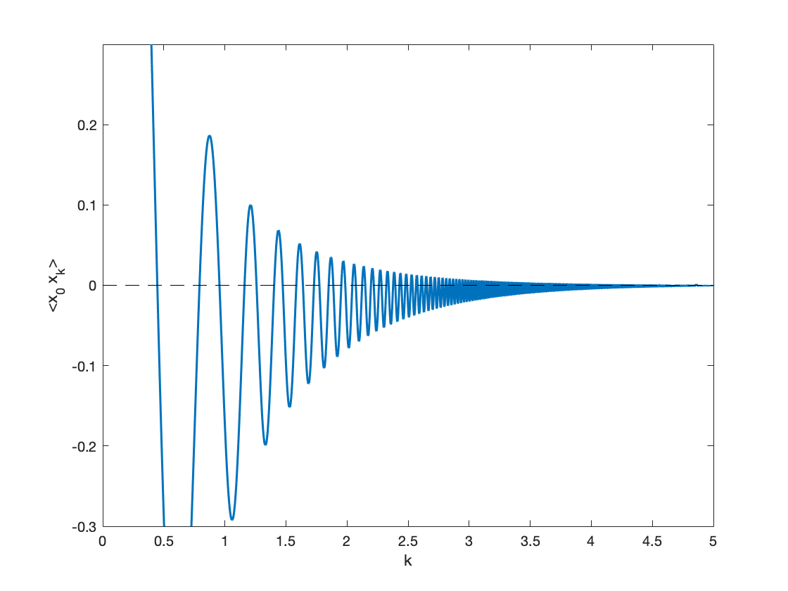
x0xkTN,π/2=12[sin(πN1+Nkπ)+sin(πN1)Nk+1+sin(Nkπ)Nk1],subscriptdelimited-⟨⟩subscript𝑥0subscript𝑥𝑘subscript𝑇𝑁𝜋212delimited-[]𝜋𝑁1superscript𝑁𝑘𝜋𝜋𝑁1superscript𝑁𝑘1superscript𝑁𝑘𝜋superscript𝑁𝑘1\langle x_{0}x_{k}\rangle_{T_{N,-\pi/2}}=-\frac{1}{2}\left[\frac{\sin\left(\frac{\pi}{N-1}+N^{k}\pi\right)+\sin\left(\frac{\pi}{N-1}\right)}{N^{k}+1}+\frac{\sin\left(N^{k}\pi\right)}{N^{k}-1}\right],

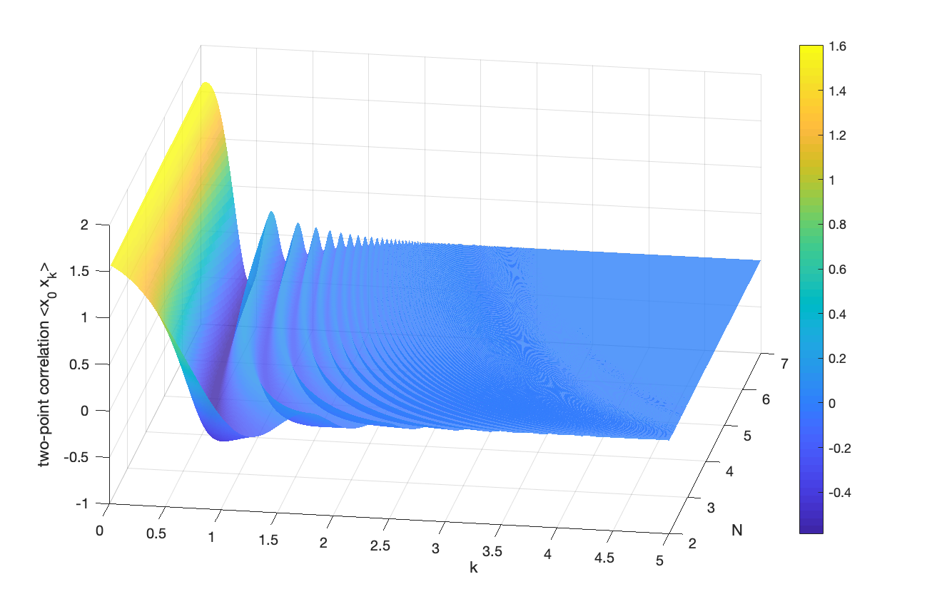
which exhibits an oscillating exponential decay in k𝑘k, cf. Fig.5.

Refer to caption
(a) x0xkTN,π/2subscriptdelimited-⟨⟩subscript𝑥0subscript𝑥𝑘subscript𝑇𝑁𝜋2\langle x_{0}x_{k}\rangle_{T_{N,-\pi/2}}, maximum is π2𝜋2\frac{\pi}{2} at k=0𝑘0k=0 for all N𝑁N
Refer to caption
(b) N=2𝑁2N=2
Refer to caption
(c) N=3𝑁3N=3
Refer to caption
(d) N=4𝑁4N=4
Figure 5: Decay of two-point correlations for TN,π2subscript𝑇𝑁𝜋2T_{N,-\frac{\pi}{2}}. Upper row: two-point correlation x0xkTN,π/2subscriptdelimited-⟨⟩subscript𝑥0subscript𝑥𝑘subscript𝑇𝑁𝜋2\langle x_{0}x_{k}\rangle_{T_{N,-\pi/2}} as a function of (k,N)[0,5]×[2,7]𝑘𝑁0527(k,N)\in[0,5]\times[2,7]. Lower row: for maps T2,π2subscript𝑇2𝜋2T_{2,-\frac{\pi}{2}}, T3,π2subscript𝑇3𝜋2T_{3,-\frac{\pi}{2}}, and T4,π2subscript𝑇4𝜋2T_{4,-\frac{\pi}{2}}, respectively.

From the results above we conclude again that already at the 2-point level, the ordinary Chebyshev maps have the lowest correlations among all the maps in the shifted Chebyshev family, and in fact also the lowest correlations as compared to any other map conjugated to an N𝑁N-ary shift.

5 Coupled map lattices (CMLs) of shifted Chebyshev maps

5.1 CMLs of two sites

We now study spatially coupled systems [11, 12, 17, 26] and investigate how the correlation patterns are modified. As the simplest model, consider a (periodic) lattice with just two sites that consists of two coupled 2nd-order ordinary Chebyshev maps:

xn+1(1)=(1c)T2,0(xn(1))+cT2,0(xn(2))xn+1(2)=(1c)T2,0(xn(2))+cT2,0(xn(1)).superscriptsubscript𝑥𝑛111𝑐subscript𝑇20superscriptsubscript𝑥𝑛1𝑐subscript𝑇20superscriptsubscript𝑥𝑛2superscriptsubscript𝑥𝑛121𝑐subscript𝑇20superscriptsubscript𝑥𝑛2𝑐subscript𝑇20superscriptsubscript𝑥𝑛1\begin{split}x_{n+1}^{(1)}&=(1-c)T_{2,0}(x_{n}^{(1)})+cT_{2,0}(x_{n}^{(2)})\\ x_{n+1}^{(2)}&=(1-c)T_{2,0}(x_{n}^{(2)})+cT_{2,0}(x_{n}^{(1)}).\end{split}

The superscript, 1 or 2, labels the spatial lattice position and the subscript n0𝑛subscript0n\in\mathbb{N}_{0} denotes a discrete time step; c[0,1]𝑐01c\in[0,1] is the coupling strength, and T2,0(x)=cos(2arccosx)=2x21subscript𝑇20𝑥2𝑥2superscript𝑥21T_{2,0}(x)=\cos(2\arccos x)=2x^{2}-1, x[1,1]𝑥11x\in[-1,1] is the 2nd-order ordinary Chebyshev map.

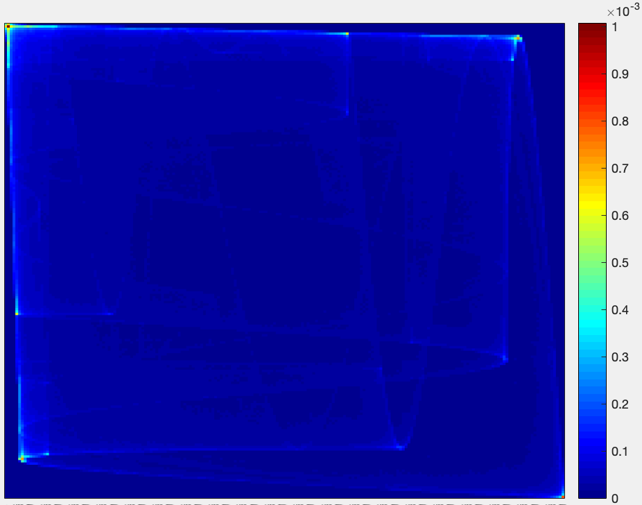
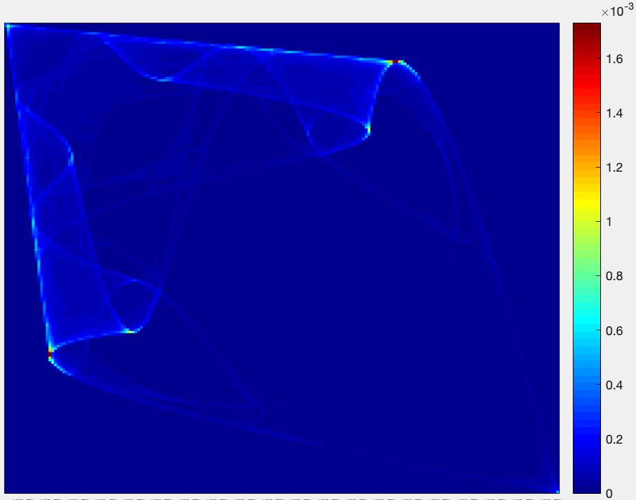
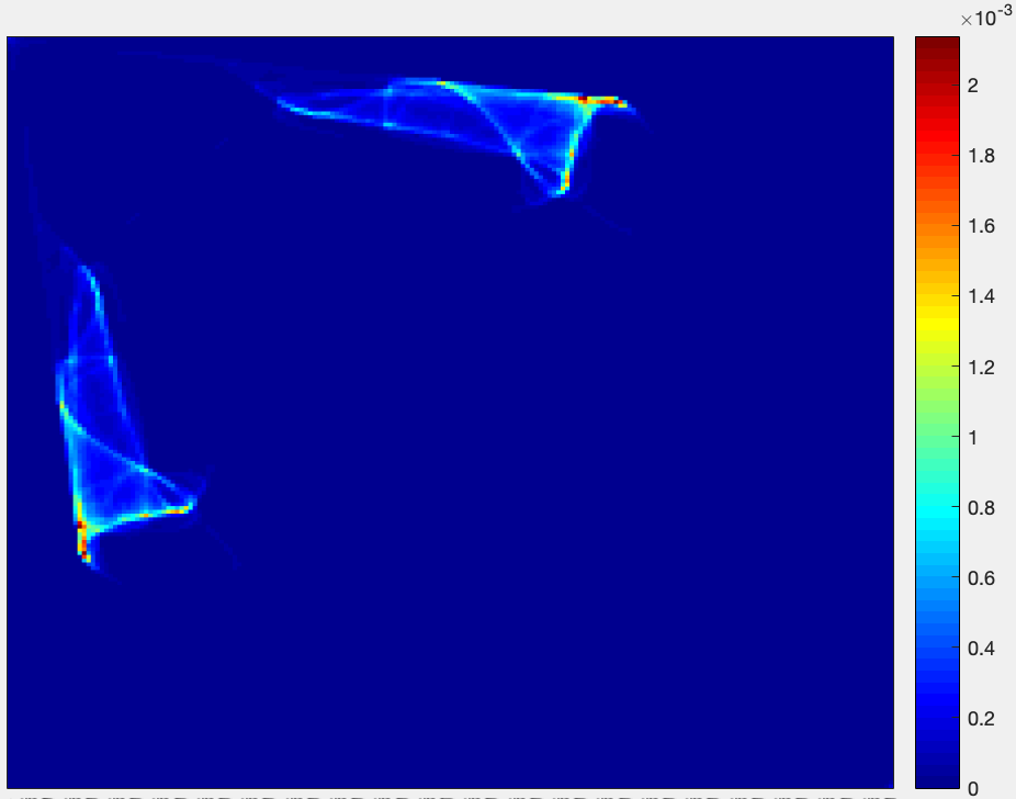
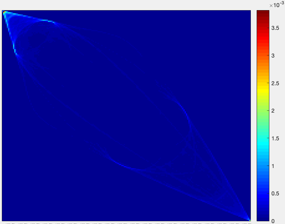
For the uncoupled case (c=0𝑐0c=0) the invariant density of the system is just the direct product of the two individual densities; as c𝑐c increases the invariant density will gradually shrink to a support given by the diagonal, that is, a total synchronisation state x(1)=x(2)superscript𝑥1superscript𝑥2x^{(1)}=x^{(2)} is approached. See Fig.6 below.

Refer to caption
(a) c=0.027𝑐0.027c=0.027
Refer to caption
(b) c=0.1𝑐0.1c=0.1
Refer to caption
(c) c=0.11𝑐0.11c=0.11
Refer to caption
(d) c=0.201𝑐0.201c=0.201
Figure 6: Heatmaps of the invariant distribution for CMLs of two sites, with different couplings indicated in each caption. The x𝑥x and y𝑦y axes are x(1)superscript𝑥1x^{(1)} and x(2)superscript𝑥2x^{(2)}, respectively (interchangeable). Colour codes the averaged probability that 10,0001000010,000 trajectories (randomly chosen initially) visit a given region over 10,100(100)1010010010,100(-100) iterations (dark blue == low probability, 200×200200200200\times 200 bins).

5.2 CMLs of many sites

For applications in quantum field theory and high energy physics it is meaningful to extend to a CML of many sites. Let T𝑇T be a one-dimensional chaotic map, and consider the following four types of coupling [4, 17]:

Type A𝐴A: forward, diffusive coupling

xn+1(i)=(1c)T(xn(i))+c2(T(xn(i1))+T(xn(i+1)))superscriptsubscript𝑥𝑛1𝑖1𝑐𝑇superscriptsubscript𝑥𝑛𝑖𝑐2𝑇superscriptsubscript𝑥𝑛𝑖1𝑇superscriptsubscript𝑥𝑛𝑖1x_{n+1}^{(i)}=(1-c)T(x_{n}^{(i)})+\frac{c}{2}\left(T(x_{n}^{(i-1)})+T(x_{n}^{(i+1)})\right)

Type Asuperscript𝐴A^{-}: forward, anti-diffusive

xn+1(i)=(1c)T(xn(i))c2(T(xn(i1))+T(xn(i+1)))superscriptsubscript𝑥𝑛1𝑖1𝑐𝑇superscriptsubscript𝑥𝑛𝑖𝑐2𝑇superscriptsubscript𝑥𝑛𝑖1𝑇superscriptsubscript𝑥𝑛𝑖1x_{n+1}^{(i)}=(1-c)T(x_{n}^{(i)})-\frac{c}{2}\left(T(x_{n}^{(i-1)})+T(x_{n}^{(i+1)})\right)

Type B𝐵B: backward, diffusive

xn+1(i)=(1c)T(xn(i))+c2(xn(i1)+xn(i+1))superscriptsubscript𝑥𝑛1𝑖1𝑐𝑇superscriptsubscript𝑥𝑛𝑖𝑐2superscriptsubscript𝑥𝑛𝑖1superscriptsubscript𝑥𝑛𝑖1x_{n+1}^{(i)}=(1-c)T(x_{n}^{(i)})+\frac{c}{2}\left(x_{n}^{(i-1)}+x_{n}^{(i+1)}\right)

Type Bsuperscript𝐵B^{-}: backward, anti-diffusive

xn+1(i)=(1c)T(xn(i))c2(xn(i1)+xn(i+1))superscriptsubscript𝑥𝑛1𝑖1𝑐𝑇superscriptsubscript𝑥𝑛𝑖𝑐2superscriptsubscript𝑥𝑛𝑖1superscriptsubscript𝑥𝑛𝑖1x_{n+1}^{(i)}=(1-c)T(x_{n}^{(i)})-\frac{c}{2}\left(x_{n}^{(i-1)}+x_{n}^{(i+1)}\right)

The superscripts i𝑖i and subscripts n𝑛n of the dynamical variable x𝑥x denote the spatial position of the lattice site and the number of iterations, respectively; c[0,1]𝑐01c\in[0,1] is the coupling strength, and T𝑇T is the local map to be specified.

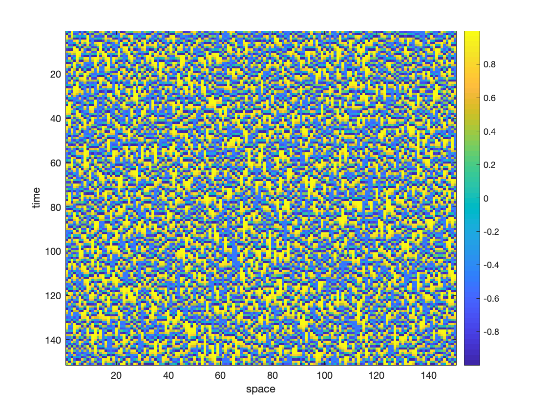
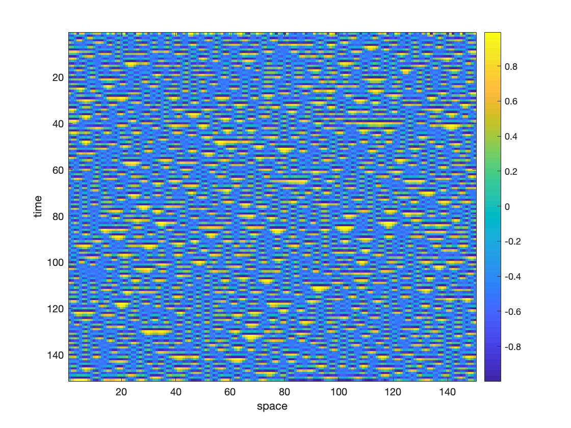
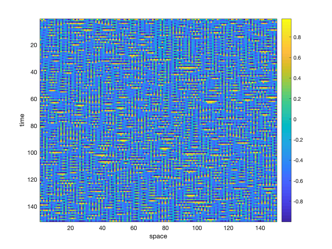
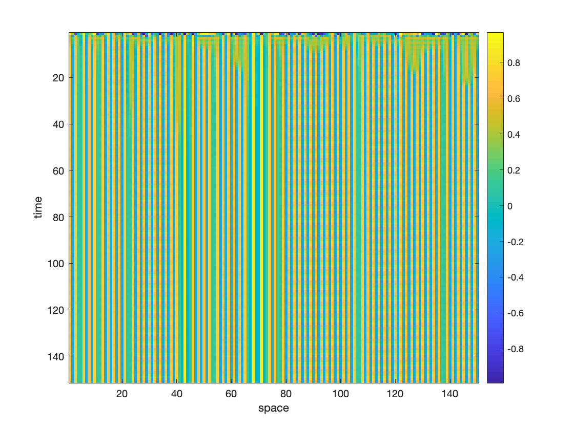
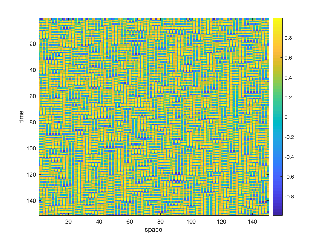
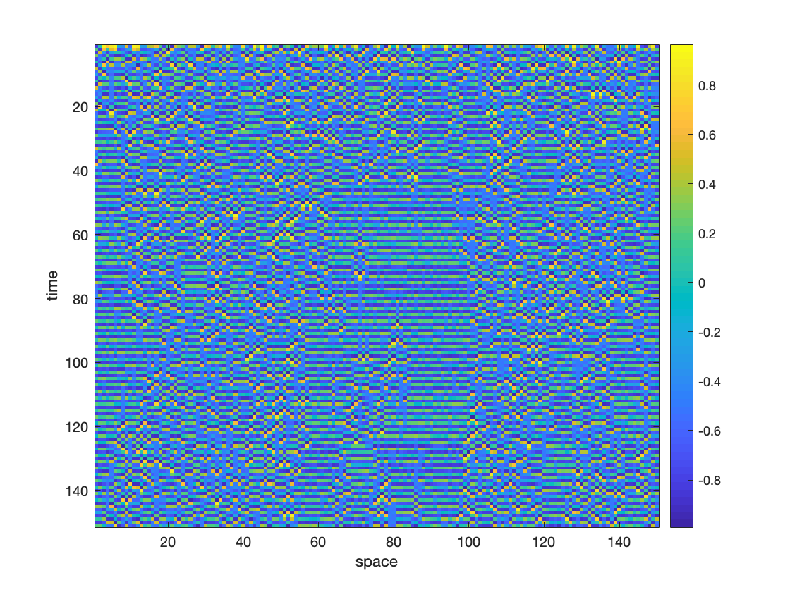
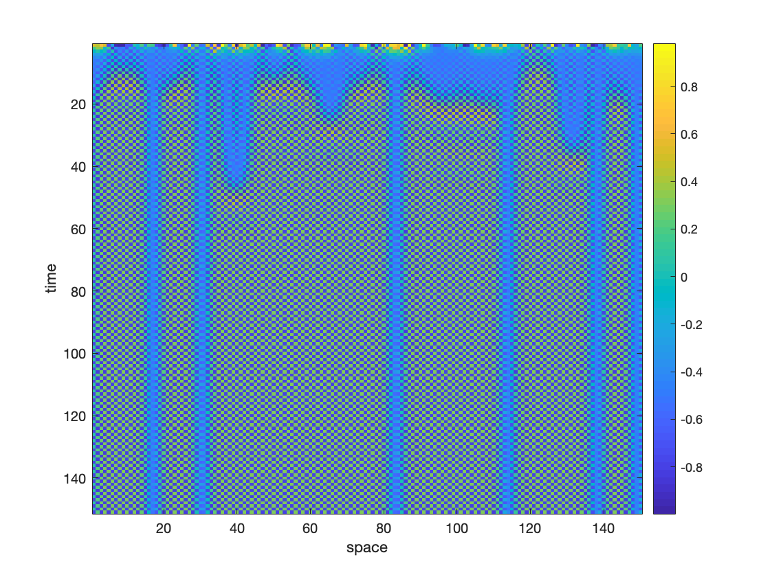
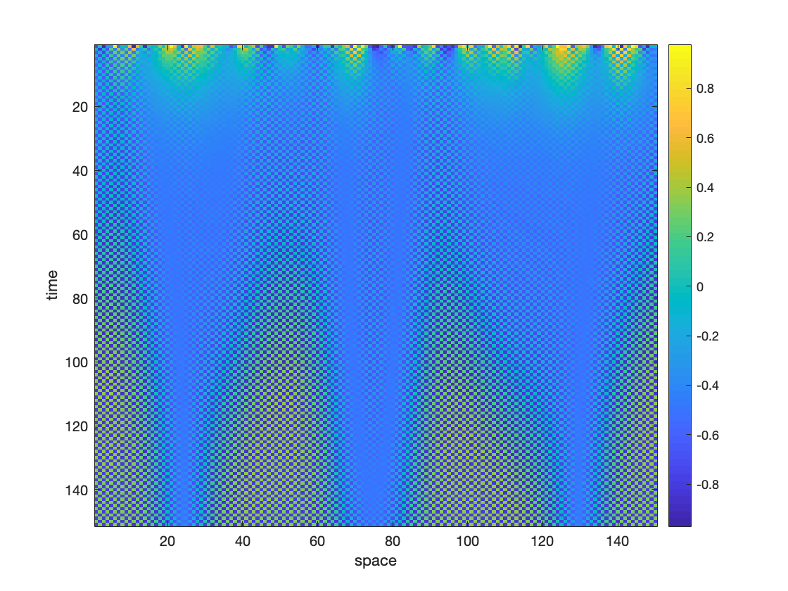
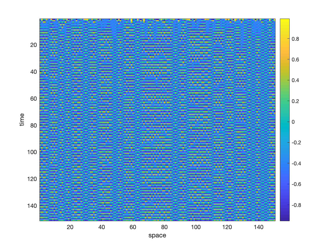
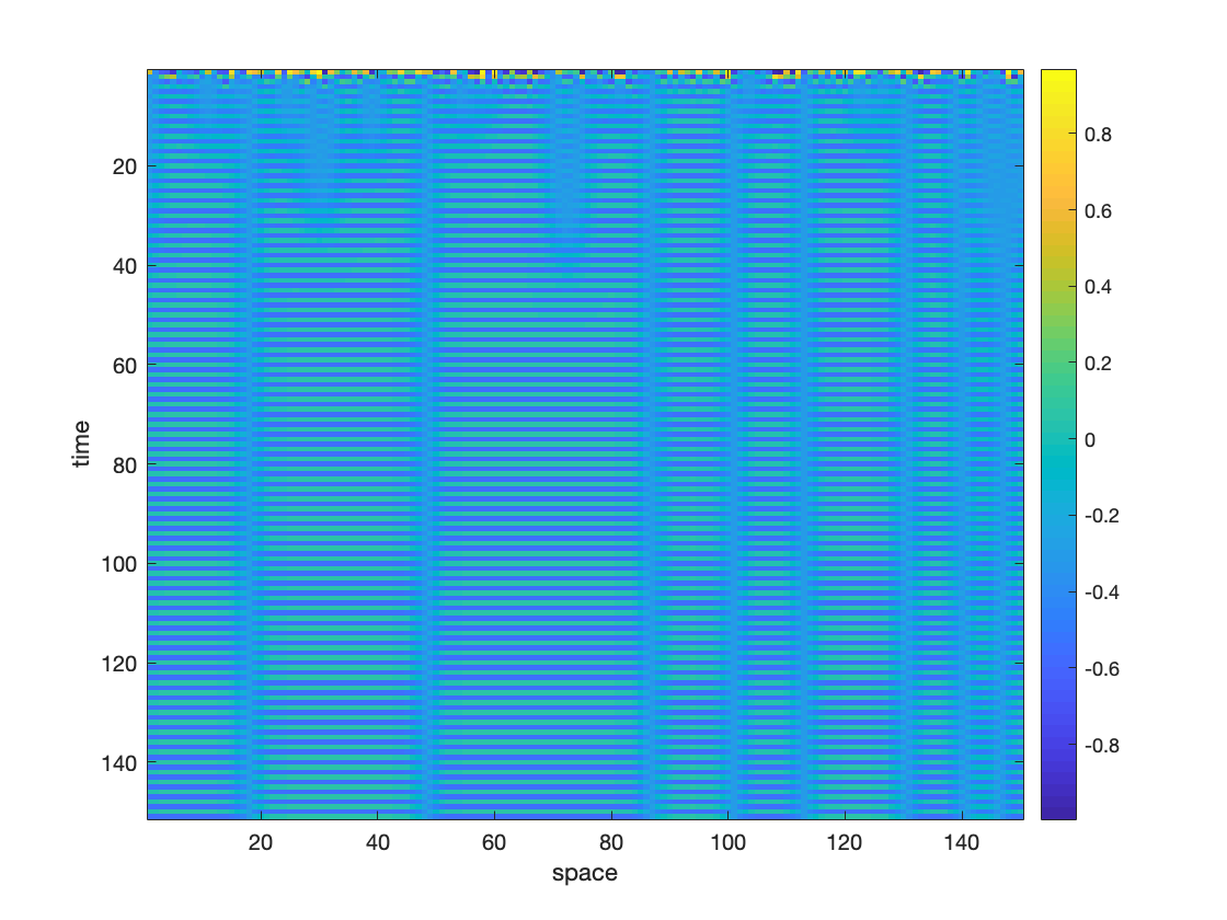
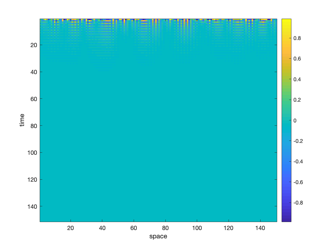
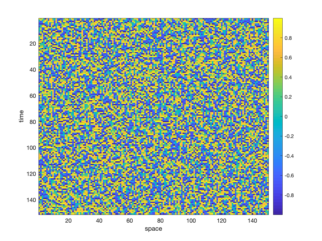
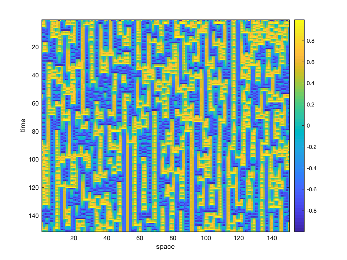
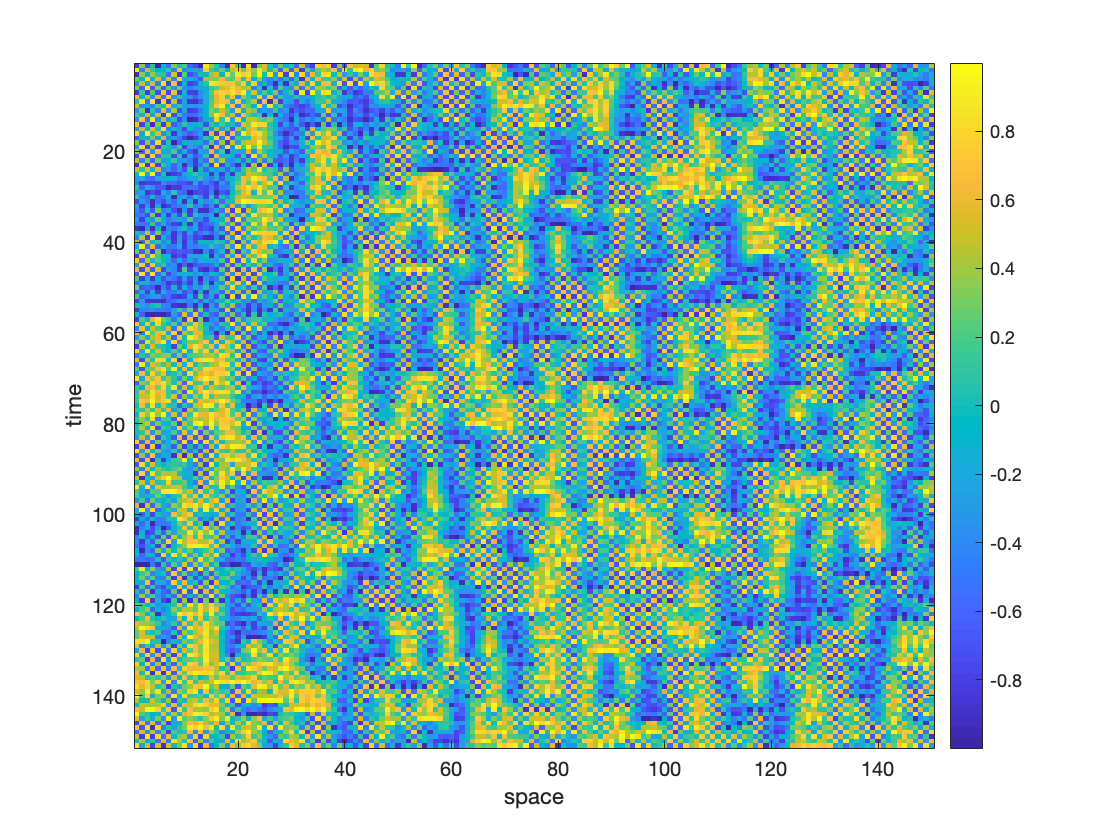
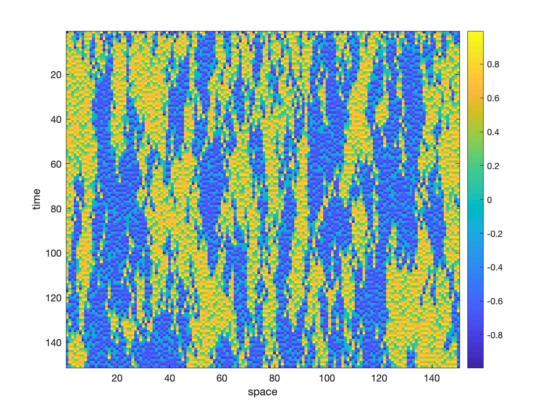
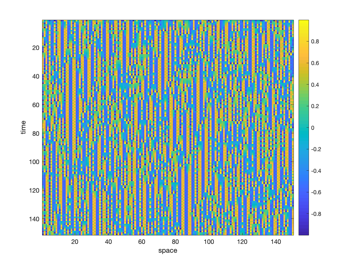
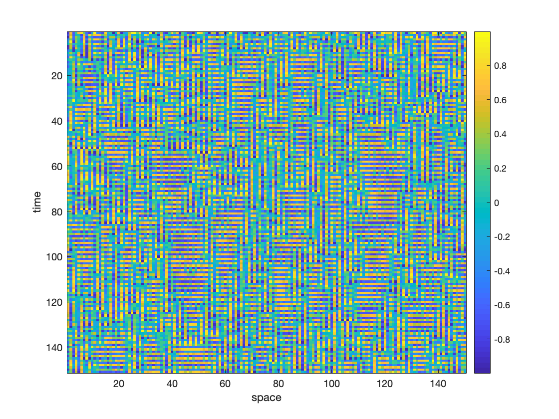
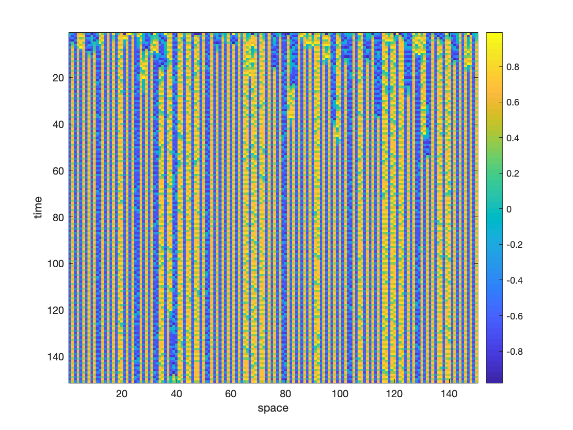
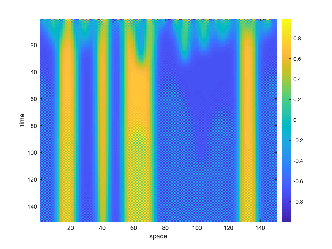
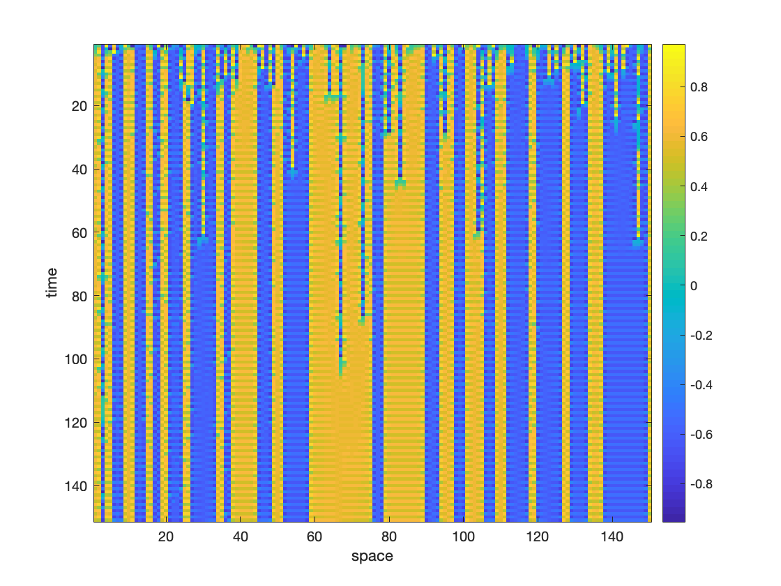
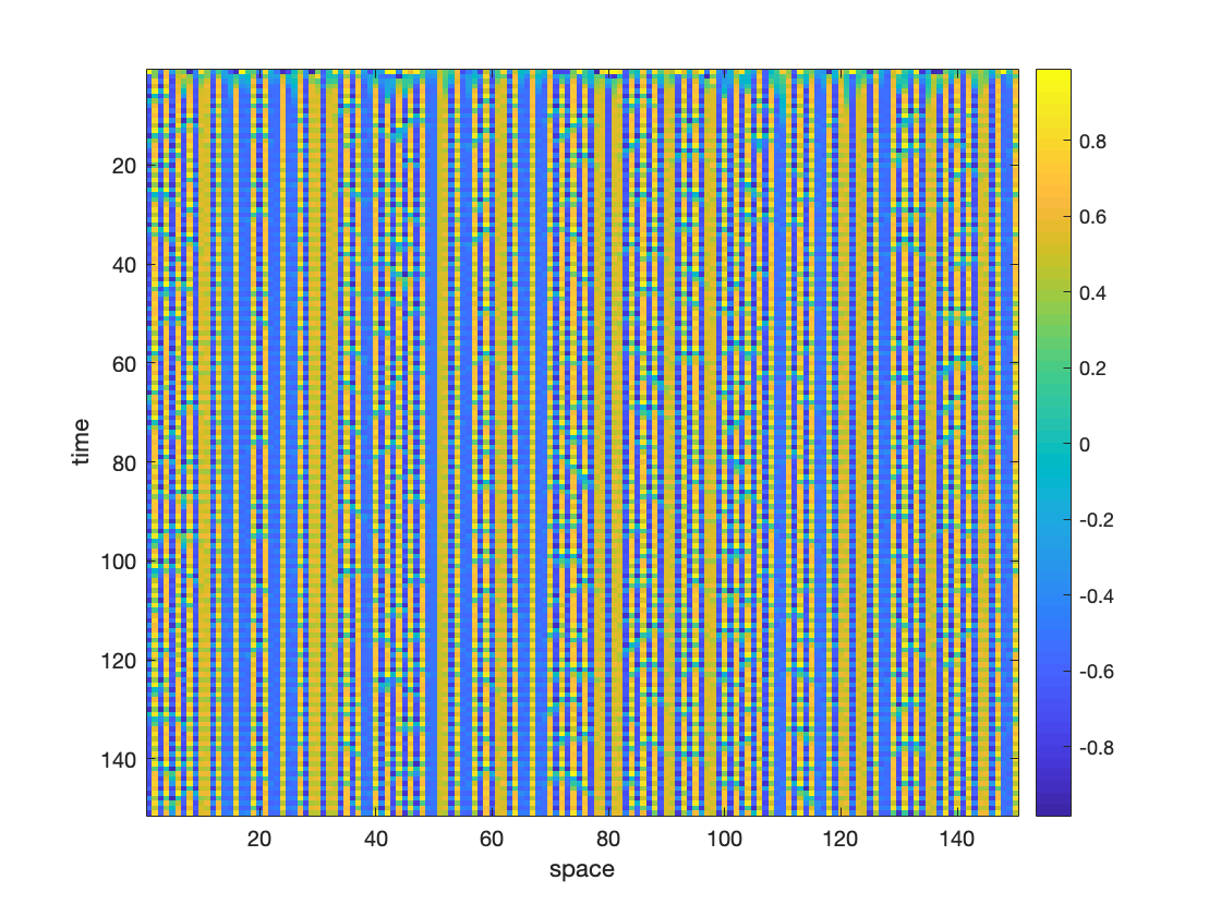
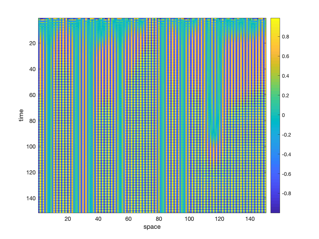
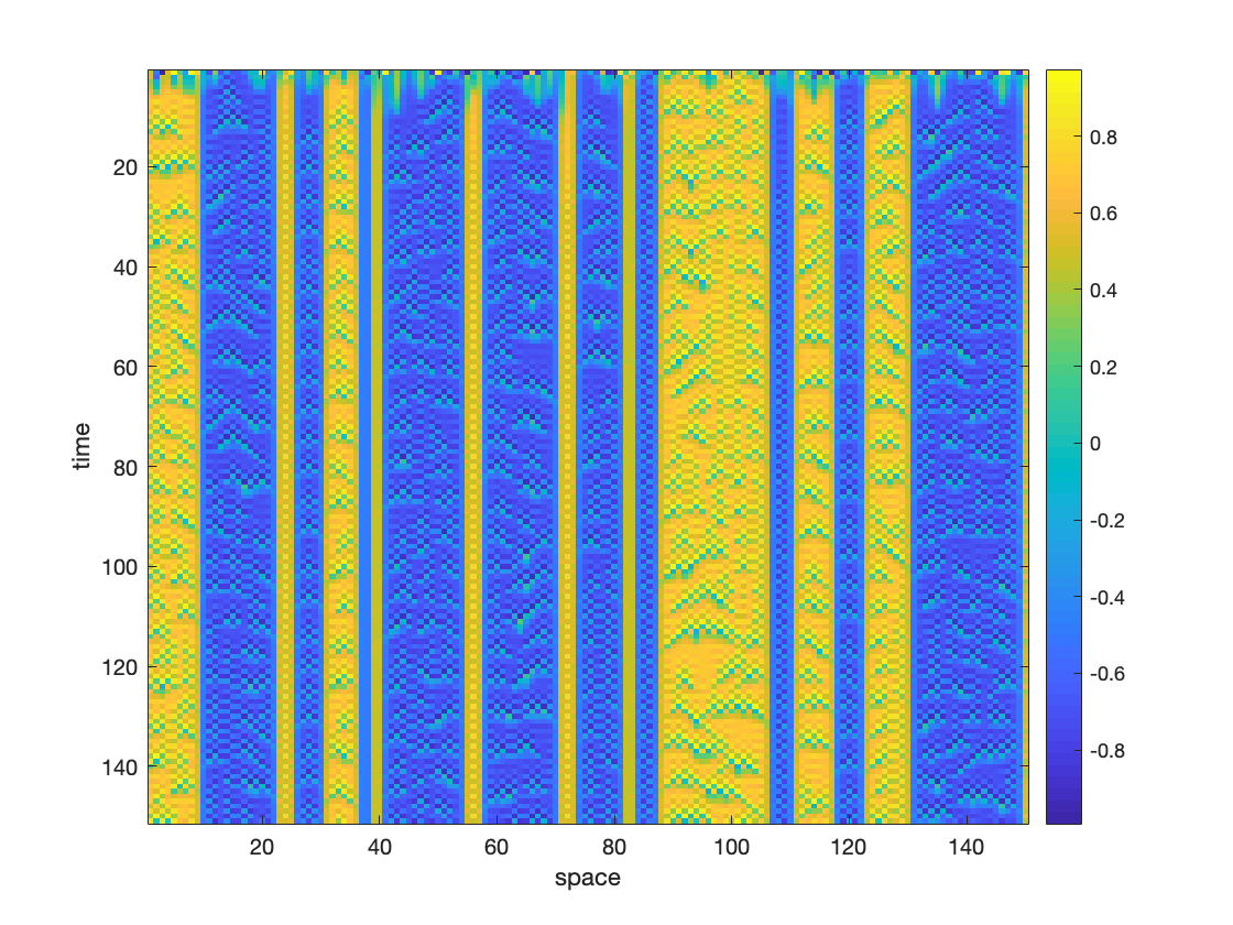
In [4] the local map T𝑇T was chosen as an ordinary Chebyshev map. To start with, consider the 2nd-order ordinary Chebyshev map T2,0(x)=cos(2arccosx)subscript𝑇20𝑥2𝑥T_{2,0}(x)=\cos(2\arccos x), x[1,1]𝑥11x\in[-1,1]. Fig.7 below shows some spatio-temporal patterns of the four types of CMLs for this local T=T2,0𝑇subscript𝑇20T=T_{2,0}. As a comparison, similar plots for local T=T3,π2𝑇subscript𝑇3𝜋2T=T_{3,-\frac{\pi}{2}} are shown in Fig.8.
Refer to caption
(a) Type 2A2𝐴2A: c=0𝑐0c=0
Refer to caption
(b) Type 2A2𝐴2A: c=0.45𝑐0.45c=0.45
Refer to caption
(c) Type 2A2𝐴2A: c=0.95𝑐0.95c=0.95
Refer to caption
(d) Type 2A2superscript𝐴2A^{-}: c=0.1𝑐0.1c=0.1
Refer to caption
(e) Type 2A2superscript𝐴2A^{-}: c=0.76𝑐0.76c=0.76
Refer to caption
(f) Type 2A2superscript𝐴2A^{-}: c=0.98𝑐0.98c=0.98
Refer to caption
(g) Type 2B2𝐵2B: c=0.13𝑐0.13c=0.13
Refer to caption
(h) Type 2B2𝐵2B: c=0.79𝑐0.79c=0.79
Refer to caption
(i) Type 2B2𝐵2B: c=0.97𝑐0.97c=0.97
Refer to caption
(j) Type 2B2superscript𝐵2B^{-}: c=0.23𝑐0.23c=0.23
Refer to caption
(k) Type 2B2superscript𝐵2B^{-}: c=0.47𝑐0.47c=0.47
Refer to caption
(l) Type 2B2superscript𝐵2B^{-}: c=0.9𝑐0.9c=0.9
Figure 7: Spatio-temporal patterns of CMLs with local T2,0subscript𝑇20T_{2,0} for increasing coupling strength. Colour encodes the value of the dynamical variable xn(i)superscriptsubscript𝑥𝑛𝑖x_{n}^{(i)}. The space×\timestime size is x×y=150×150𝑥𝑦150150x\times y=150\times 150; on each lattice site i𝑖i the initial value is randomly chosen as x0(i)Uni(1,1)superscriptsubscript𝑥0𝑖Uni11x_{0}^{(i)}\in\text{Uni}(-1,1), with periodic boundary conditions.
Refer to caption
(a) Type 3A3𝐴3A: c=0𝑐0c=0
Refer to caption
(b) Type 3A3𝐴3A: c=0.45𝑐0.45c=0.45
Refer to caption
(c) Type 3A3𝐴3A: c=0.95𝑐0.95c=0.95
Refer to caption
(d) Type 3A3superscript𝐴3A^{-}: c=0.11𝑐0.11c=0.11
Refer to caption
(e) Type 3A3superscript𝐴3A^{-}: c=0.36𝑐0.36c=0.36
Refer to caption
(f) Type 3A3superscript𝐴3A^{-}: c=0.91𝑐0.91c=0.91
Refer to caption
(g) Type 3B3𝐵3B: c=0.19𝑐0.19c=0.19
Refer to caption
(h) Type 3B3𝐵3B: c=0.52𝑐0.52c=0.52
Refer to caption
(i) Type 3B3𝐵3B: c=0.92𝑐0.92c=0.92
Refer to caption
(j) Type 3B3superscript𝐵3B^{-}: c=0.24𝑐0.24c=0.24
Refer to caption
(k) Type 3B3superscript𝐵3B^{-}: c=0.49𝑐0.49c=0.49
Refer to caption
(l) Type 3B3superscript𝐵3B^{-}: c=0.93𝑐0.93c=0.93
Figure 8: Spatio-temporal patterns of CMLs with local T3,π2subscript𝑇3𝜋2T_{3,-\frac{\pi}{2}}; same iteration parameters as in Fig.7.

A variety of interesting patterns is generated, such as turbulent-like behaviour (Fig.7g), intermittency (Fig.8b), and frozen chaos (Fig.8k); see e.g.[26] for a characterisation of different phenomena. Some of the patterns remind us of biological structures: Figs.8c, 8d resemble some self-organised patches in nature or ecosystems, such as kelps and duckweeds.

5.3 Spatial and temporal correlation functions

Our main interest in this paper is to quantify the correlation structure. For CMLs, two different types of correlations occur, namely in the spatial direction and in the temporal direction. Let us define the SNNC𝑆𝑁𝑁𝐶SNNC (spatial nearest-neighbour correlation) and the TNNC𝑇𝑁𝑁𝐶TNNC (temporal nearest-neighbour correlation) as the following averages:

SNNC=limK1KJn=1Kj=1Jxn(j)xn(j+1),TNNC=limK1JKj=1Jn=1Kxn(j)xn+1(j).formulae-sequence𝑆𝑁𝑁𝐶subscript𝐾1𝐾𝐽superscriptsubscript𝑛1𝐾superscriptsubscript𝑗1𝐽superscriptsubscript𝑥𝑛𝑗superscriptsubscript𝑥𝑛𝑗1𝑇𝑁𝑁𝐶subscript𝐾1𝐽𝐾superscriptsubscript𝑗1𝐽superscriptsubscript𝑛1𝐾superscriptsubscript𝑥𝑛𝑗superscriptsubscript𝑥𝑛1𝑗\begin{split}SNNC&=\lim_{K\rightarrow\infty}\frac{1}{KJ}\sum_{n=1}^{K}\sum_{j=1}^{J}x_{n}^{(j)}x_{n}^{(j+1)},\\ TNNC&=\lim_{K\rightarrow\infty}\frac{1}{JK}\sum_{j=1}^{J}\sum_{n=1}^{K}x_{n}^{(j)}x_{n+1}^{(j)}.\end{split} (7)

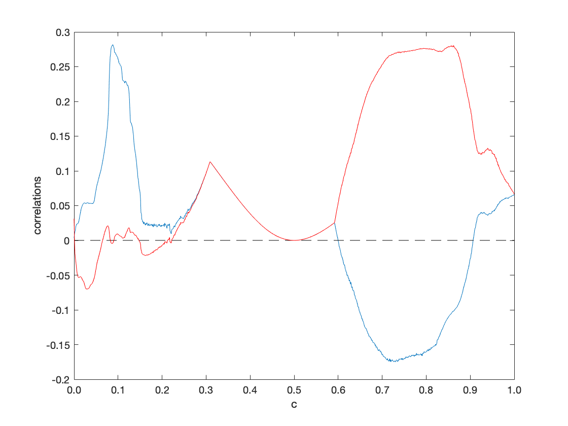
For finite K𝐾K and J𝐽J the order of the two sums is interchangeable. In practice, we are interested in very large values of K𝐾K and J𝐽J, and in particular in the limit K𝐾K\to\infty, corresponding to the long-term iteration limit, where the system (if ergodic) may again approach an invariant density, which for the CML is a function of J𝐽J different variables. In the following, we show some numerical results for the above observables, SNNC𝑆𝑁𝑁𝐶SNNC and TNNC𝑇𝑁𝑁𝐶TNNC, as a function of the parameters c𝑐c and a𝑎a.

(i) CML of Type 2A2𝐴2A:

Refer to caption
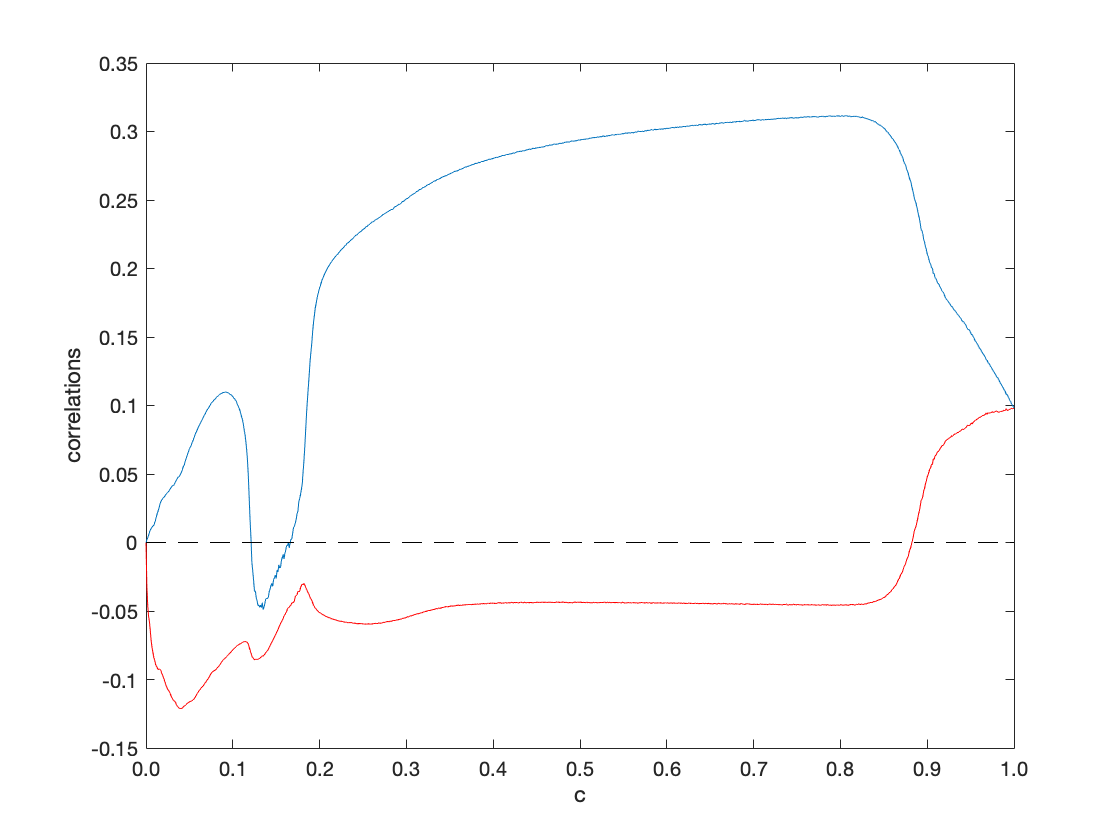
(a) SNNC𝑆𝑁𝑁𝐶SNNC (blue) and TNNC𝑇𝑁𝑁𝐶TNNC (red) at a=0𝑎0a=0
Refer to caption
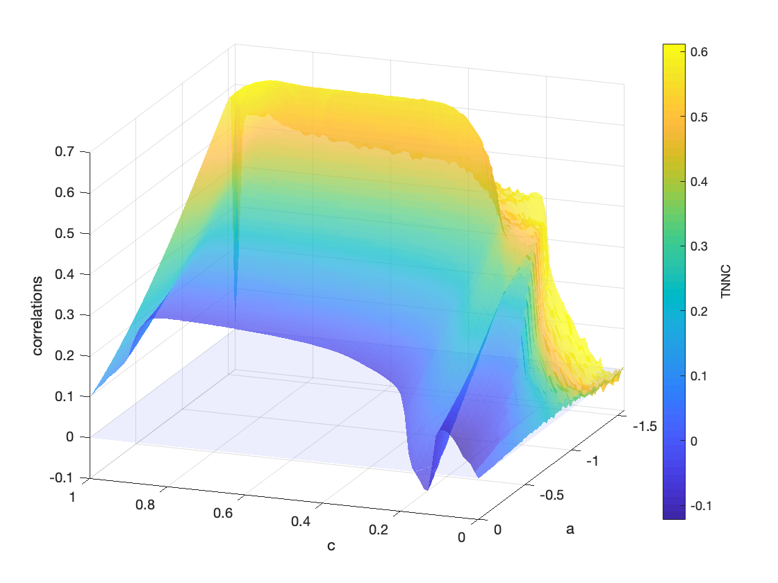
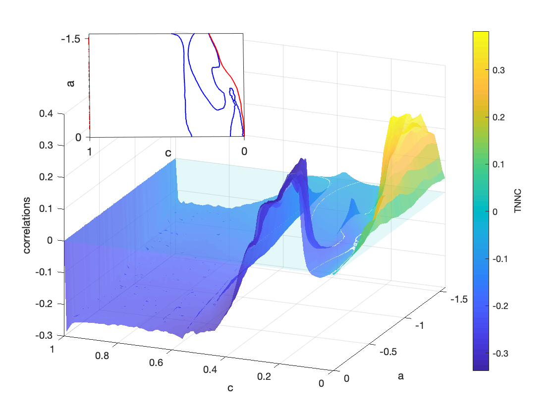
(b) SNNC𝑆𝑁𝑁𝐶SNNC (z-height) and TNNC𝑇𝑁𝑁𝐶TNNC (coloured)
Figure 9: SNNC𝑆𝑁𝑁𝐶SNNC and TNNC𝑇𝑁𝑁𝐶TNNC for Type 2A2𝐴2A CML: c[0,1]𝑐01c\in[0,1], a[π2,0]𝑎𝜋20a\in\left[-\frac{\pi}{2},0\right]. The space×\timestime size is J×K=5,000×1,100(100)𝐽𝐾50001100100J\times K=5,000\times 1,100(-100); initial points randomly chosen from a uniform distribution Uni(1,1)11(-1,1).

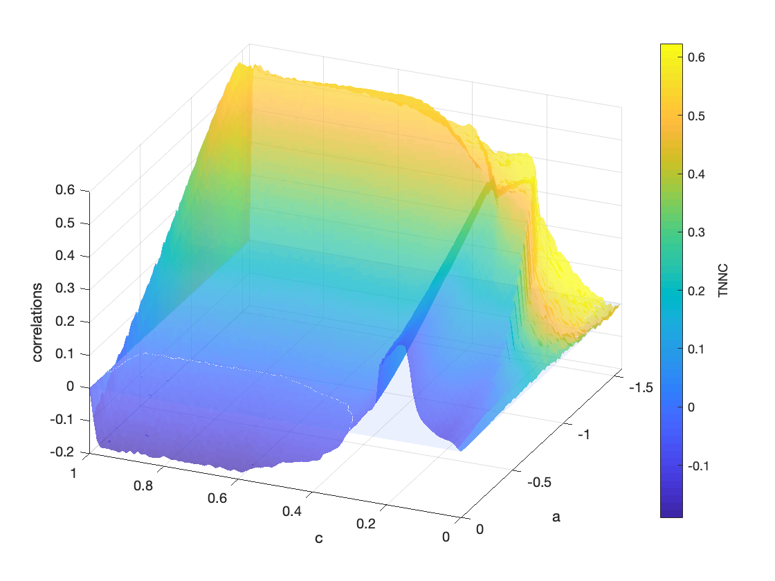
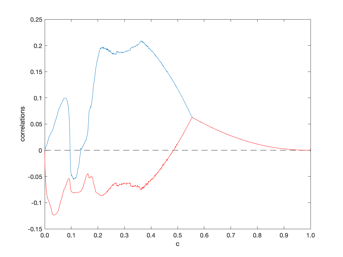
Notice that in the correlation surface plot, there is a rapid folding around c[0.1,0.2]𝑐0.10.2c\in[0.1,0.2], creating two distinct zeros of SNNC𝑆𝑁𝑁𝐶SNNC depending on a𝑎a. Fluctuations as c0𝑐0c\rightarrow 0 with aπ2𝑎𝜋2a\rightarrow-\frac{\pi}{2} indicate that the system loses its ergodic property and that the averaged correlation fails to stabilise, which could be induced by non-mixing of the underlying system. These fluctuation regions, depending on both the coupling c𝑐c and the shift parameter a𝑎a, are very intricate, and occur for other coupling forms as well.

For a=0𝑎0a=0 we observe special coupling parameter values (such as c0.12similar-to𝑐0.12c\sim 0.12) where SNNC=0𝑆𝑁𝑁𝐶0SNNC=0, see [4] for a physical interpretation in a quantum field theoretical setting. There are also special values (such as c0.88similar-to𝑐0.88c\sim 0.88) where TNNC=0𝑇𝑁𝑁𝐶0TNNC=0. This means that although there is non-trivial spatial coupling, some features of the uncoupled (most random-looking) local Chebyshev dynamics are restored for these special coupling constants.

(ii) CML of Type 2A2superscript𝐴2A^{-}:

Refer to caption
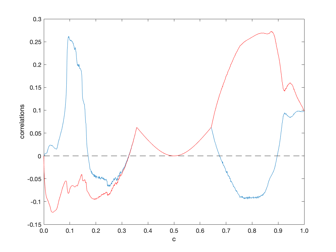
(a) SNNC𝑆𝑁𝑁𝐶SNNC (blue) and TNNC𝑇𝑁𝑁𝐶TNNC (red) at a=0𝑎0a=0
Refer to caption
(b) SNNC𝑆𝑁𝑁𝐶SNNC (z-height) and TNNC𝑇𝑁𝑁𝐶TNNC (coloured)
Figure 10: Same as in Fig.9 except for Type 2A2superscript𝐴2A^{-}.
Refer to caption
(a) a=π/16𝑎𝜋16a=-\pi/16
Refer to caption
(b) a=π/8𝑎𝜋8a=-\pi/8
Refer to caption
(c) a=3π/16𝑎3𝜋16a=-3\pi/16
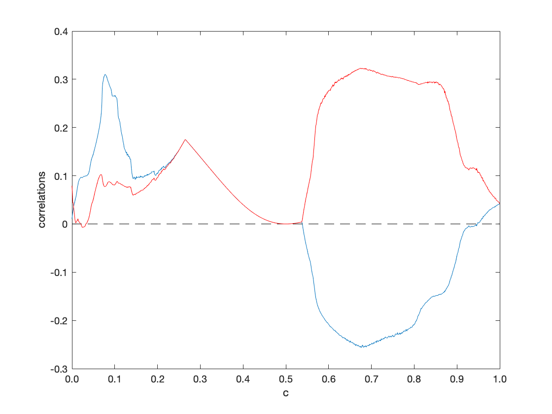
Figure 11: SNNC𝑆𝑁𝑁𝐶SNNC (blue) and TNNC𝑇𝑁𝑁𝐶TNNC (red) for Type 2A2superscript𝐴2A^{-} at a=π/16𝑎𝜋16a=-\pi/16, π/8𝜋8-\pi/8 and 3π/163𝜋16-3\pi/16, c[0,1]𝑐01c\in[0,1]. Other parameters are the same as in Fig.9.

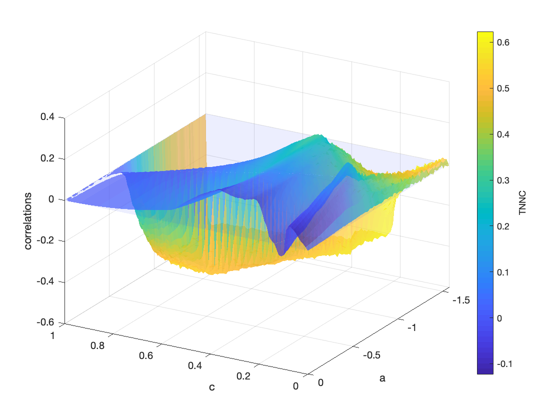
Here in most parts the SNNC𝑆𝑁𝑁𝐶SNNC is negative while TNNC𝑇𝑁𝑁𝐶TNNC keeps growing as aπ2𝑎𝜋2a\rightarrow-\frac{\pi}{2}. The parabola-like curve starting at (c,a)=(0.5,0)𝑐𝑎0.50(c,a)=(0.5,0) is due to a stable synchronised fixed point of the CML, as a simple stability analysis shows, and it disappears when a>0.45𝑎0.45a>0.45, see Fig.11 for more detail.

(iii) CML of Type 2B2𝐵2B:

Refer to caption
(a) SNNC𝑆𝑁𝑁𝐶SNNC (blue) and TNNC𝑇𝑁𝑁𝐶TNNC (red) at a=0𝑎0a=0
Refer to caption
(b) SNNC𝑆𝑁𝑁𝐶SNNC (z-height) and TNNC𝑇𝑁𝑁𝐶TNNC (coloured)
Figure 12: Same as in Fig.9 except for Type 2B2𝐵2B.

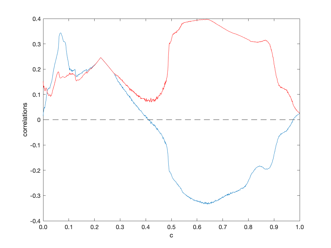
For small c𝑐c the correlation surface is similar as for Type 2A2𝐴2A: there also exists a rapid folding near c=0.15𝑐0.15c=0.15. In contrast to types 2A2superscript𝐴2A^{-} and 2B2superscript𝐵2B^{-}, there exists no stable synchronised fixed point state for larger c𝑐c.

(iv) CML of Type 2B2superscript𝐵2B^{-}:

Refer to caption
(a) SNNC𝑆𝑁𝑁𝐶SNNC (blue) and TNNC𝑇𝑁𝑁𝐶TNNC (red) at a=0𝑎0a=0
Refer to caption
(b) SNNC𝑆𝑁𝑁𝐶SNNC (z-height) and TNNC𝑇𝑁𝑁𝐶TNNC (coloured)
Figure 13: Same as in Fig.9 except for Type 2B2superscript𝐵2B^{-}.

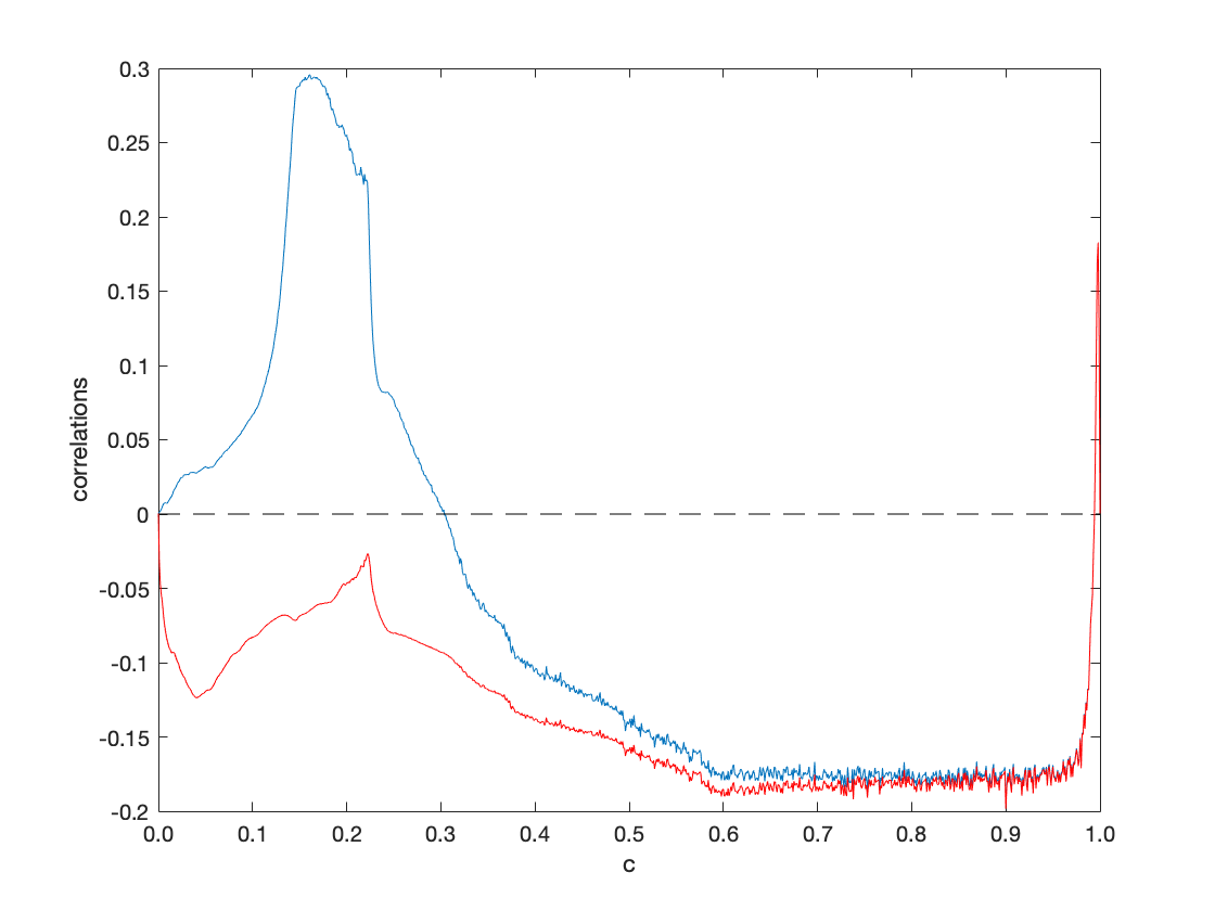
Yet another type of coupling form relevant in quantum field theoretical applications. For c1𝑐1c\to 1 and small a𝑎a we observe a stable synchronised fixed point. In general, as outlined in more detail in [4], physical interaction states correspond to zeros of SNNC𝑆𝑁𝑁𝐶SNNC.

Finally, let us also consider coupled Chebyshev maps with odd N𝑁N, which have a different symmetry behaviour: for odd N𝑁N coupled Chebyshev systems, the average of the iterates is always zero, whereas for even N𝑁N it is not.

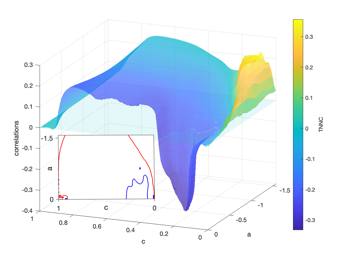
The coloured plots in Fig.14 below show the SNNC𝑆𝑁𝑁𝐶SNNC (z-height) and TNNC𝑇𝑁𝑁𝐶TNNC (encoded in colour) for types 3A3𝐴3A and 3B3𝐵3B CMLs (i.e., the local map is T=T3,0𝑇subscript𝑇30T=T_{3,0}). For Type 3A3𝐴3A there is a dip in the spatial correlation (SNNC𝑆𝑁𝑁𝐶SNNC) when a𝑎a is close to 00 with weak coupling c𝑐c; while for Type 3B3𝐵3B a jump in SNNC𝑆𝑁𝑁𝐶SNNC occurs around the same parameter region, and when c>0.5𝑐0.5c>0.5 again fluctuations caused by non-mixing are prevalent. The temporal correlation (TNNC𝑇𝑁𝑁𝐶TNNC) is increasing when |a|𝑎|a| becomes larger.

Overall, we notice that spatial coupling destroys the simple, distinguished correlation properties of Chebyshev maps, as visible already for the nearest neighbour-correlation in space and time, which was identical to zero for a=0𝑎0a=0 with c=0𝑐0c=0. Still, some distinguished non-trivial parameter values exist in the (c,a)𝑐𝑎(c,a)-plane which generate uncorrelated nearest-neighbour behaviour. As an example, subplots in Fig.14 indicate the special curves in the (c,a)𝑐𝑎(c,a)-plane where SNNC=0𝑆𝑁𝑁𝐶0SNNC=0 (blue) and TNNC=0𝑇𝑁𝑁𝐶0TNNC=0 (red) for both 3A3𝐴3A and 3B3𝐵3B coupling forms.

Refer to caption
(a) Type 3A3𝐴3A
Refer to caption
(b) Type 3B3𝐵3B
Figure 14: SNNC𝑆𝑁𝑁𝐶SNNC (z-height) and TNNC𝑇𝑁𝑁𝐶TNNC (coloured) for types 3A3𝐴3A and 3B3𝐵3B: c[0,1]𝑐01c\in[0,1], a[π2,0]𝑎𝜋20a\in\left[-\frac{\pi}{2},0\right], with subplots showing zeros of SNNC𝑆𝑁𝑁𝐶SNNC (blue) and TNNC𝑇𝑁𝑁𝐶TNNC (red). Other parameters are the same as in Fig.9.

6 Conclusion

In this paper we have shown that Chebyshev maps, among all maps conjugated to a shift dynamics of N𝑁N symbols, are very distinguished dynamical systems. They generate least higher-order correlations, and can thus be regarded as the most random-looking systems, among all possible dynamical systems, assuming a deterministic evolution dynamics as given given by a smooth differentiable one-dimensional map conjugated to an N𝑁N-ary shift. We generalised the concept and were able to determine invariant densities for shifted Chebyshev maps as well, which are a modification of the ordinary Chebyshev map described by a translation parameter a𝑎a. For particular values of the parameters N𝑁N and a𝑎a we were able to determine the entire (discrete) set of eigenfunctions of the Perron-Frobenius operator.

There are several aspects of evidence that the (ordinary, a=0𝑎0a=0) Chebyshev maps are distinguished among other deterministic chaotic systems under consideration. First of all, for iterates of an uncoupled Chebyshev map, the two-point correlation decays very fast — described by a Kronecker delta function — indicating that it vanishes immediately instead of exponentially such as for an N𝑁N-ary shift map with subtracted mean; zeros of higher-order correlations can be determined by diophantine equations with the simplest possible spin configurations, namely up-down spin space; other dynamical systems correspond to a more complicated integer-spin space that is embedded in the generalised diophantine equations we considered in this paper.

It is also remarkable that for Chebyshev maps an orthogonal set of eigenfunctions of the Perron-Frobenius operator exists, and that the eigenvalues are real, in spite of the fact that the operator itself is not Hermitean. We were able to find the eigenfunctions also for the generalised shifted Chebyshev maps, in the case of even N𝑁N. The observation here is that a conjugating function h1subscript1h_{1} can be found which relates the dynamics of shifted Chebyshev maps to that of ordinary Chebyshev maps, in particular, h1subscript1h_{1} is simply a negative (ordinary) Chebyshev polynomial whose order depends on the translation parameter a𝑎a.

When a spatial coupling c0𝑐0c\not=0 is introduced, the simple Bernoulli shift properties of shifted Chebyshev maps are destroyed in the corresponding coupled map lattice. However, numerically still some distinguished coupling constants can be found where the spatial nearest-neighbour correlation of the coupled map lattice vanishes. This means that in spite of the non-zero coupling, still a random-like correlation state can be achieved. These types of states have physical meaning in chaotically quantized field theories, fixing allowed types of coupling constants, and making contact to observed coupling constants in the standard model of elementary particle physics [4, 17]. Our consideration in this paper has shown that indeed Chebyshev maps are the most distinguished dynamical systems, in the sense that they allow to construct a most random-like looking chaotic field theory, which at the microscopic level is purely deterministic.

References

  • [1] A. Boyarsky and P. Gora, Laws of Chaos: Invariant Measures and Dynamical Systems in One Dimension, Birkhauser (1997)
  • [2] A. Hilgers and C. Beck, Higher-order correlations of Tchebyscheff maps, Physica D 156 1-18 (2001)
  • [3] C. Beck, Higher correlation functions of chaotic dynamical systems – a graph theoretical approach, Nonlinearity 4, 1131-1158 (1991)
  • [4] C. Beck, Spatio-Temporal Chaos and Vacuum Fluctuations of Quantized Fields, Advanced Series in Nonlinear Dynamics Vol.21, World Scientific (2002)
  • [5] C. Beck and F. Schlögl, Thermodynamics of Chaotic Systems: an introduction, Cambridge Nonlinear Science Series (2005)
  • [6] G. Froyland, Extracting Dynamical Behaviour via Markov Models, Nonlinear Dynamics and Statistics. Birkhauser, Boston, MA (2001)
  • [7] L. Vepstas, The Bernoulli Operator (2014)
  • [8] T. Bedford, M. Keane, and C. Series, Ergodic Theory, Symbolic Dynamics, and Hyperbolic Spaces, Oxford University Press (1991)
  • [9] R.L. Adler and T.J. Rivlin, Ergodic and mixing properties of Chebyshev polynomials, Proc. Am. Math. Soc. 15, 794 (1964)
  • [10] T. Geisel and V. Fairen, Statistical properties of chaos in Chebyshev maps, Phys. Lett. A 105, 263-266 (1984)
  • [11] C.P. Dettmann and D. Lippolis, Periodic orbit theory of two coupled Tschebycheff maps, Chaos Sol. Fractals 23, 43-54 (2005)
  • [12] S. Groote and H. Vermäe, Short chaotic strings and their behaviour in the scaling region, Chaos Sol. Fractals 41, 2354-2359 (2009)
  • [13] G. Williams and C. Beck, Stochastic differential equations driven by deterministic chaotic maps: Analytic solutions of the Perron-Frobenius equation, Nonlinearity 31, 3484 (2018)
  • [14] C. Beck and G. Roepstorff, From dynamical systems to the Langevin equation, Physica A 145, 1 (1987)
  • [15] I. Melbourne and A.M. Stuart, A note on diffusion limits of chaotic skew product flows, Nonlinearity 24, 1361 (2011)
  • [16] M.C. Mackey and M. Tyran-Kaminska, Central limit theorem behaviour in the skew tent map, Chaos Sol. Fractals 38, 789-805 (2008)
  • [17] C. Beck, Chaotic strings and standard model parameters, Physica D 171, 72 (2002)
  • [18] C. Beck, Chaotic quantization of field theories, Nonlinearity 8, 423 (1995)
  • [19] A. Lasota and M.C. Mackey, Probabilistic Properties of Deterministic Systems, Cambridge University Press (1985)
  • [20] V. Baladi, Positive Transfer Operators and Decay of Correlations, Advanced Series in Nonlinear Dynamics Vol.16, World Scientific (2000)
  • [21] M. Pollicott, A complex Ruelle-Perron-Frobenius theorem and two counterexamples, Ergod. Th. Dyn. Syst. 4, 135-146 (1984)
  • [22] M. Doerfle, Spectrum and Eigenfunctions of the Frobenius-Perron Operator of the Tent Map, Journal of Statistical Physics 40, 93-132 (1985)
  • [23] U. Tirnakli and E. Borges, The standard map: From Boltzmann-Gibbs statistics to Tsallis statistics, Scientific Rep. 6, 23644 (2016)
  • [24] A. Bountis, J.J.P. Veerman and F. Vivaldi, Cauchy distributions for the integrable standard map, arXiv:2004.12912 (2020)
  • [25] U. Tirnakli, C. Beck and C. Tsallis, Central limit behaviour of deterministic dynamical systems, Phys. Rev. E 75, 040106 (2007)
  • [26] K. Kaneko, Theory and Applications of Coupled Map Lattices, Wiley (1995)
  • [27] Donald E. Knuth, Johann Faulhaber and sums of powers, Maths and Comp. 61, 277-294 (1993)

Appendix A Proof of topological conjugation between shifted Chebyshev maps and piecewise-linear maps

Let us denote X=[1,1]𝑋11X=[-1,1], Y=[0,1]𝑌01Y=[0,1]. The shifted Chebyshev maps TN,a:XX:subscript𝑇𝑁𝑎𝑋𝑋T_{N,a}:X\rightarrow X are defined as TN,a(x)=cos(Narccosx+a)subscript𝑇𝑁𝑎𝑥𝑁𝑥𝑎T_{N,a}(x)=\cos(N\arccos x+a), with the two parameters N2𝑁subscriptabsent2N\in\mathbb{N}_{\geq 2} and a[π2,0]𝑎𝜋20a\in\left[-\frac{\pi}{2},0\right]. The piecewise-linear maps gN,a:YY:subscript𝑔𝑁𝑎𝑌𝑌g_{N,a}:Y\rightarrow Y are defined like a multi-tent or multi-upside-down tent map with piecewise constant slope ±Nplus-or-minus𝑁\pm N (cf. Fig.4). Here we only consider N=2𝑁2N=2 as an example; for a general N2𝑁subscriptabsent2N\in\mathbb{N}_{\geq 2} the proof follows the same method (but one needs to distinguish odd and even N𝑁N cases). Denote

f(x)=T2,a(x)=cos(2arccosx+a),xX=[1,1]g(y)=g2,a(y)={2y+α,y[0,1α2)=:Y12y+2α,y[1α2,2α2)=:Y22y+α2,y[2α2,1]=:Y3\begin{split}f(x)&=T_{2,a}(x)=\cos(2\arccos x+a),\quad x\in X=[-1,1]\\ g(y)&=g_{2,a}(y)=\begin{cases}2y+\alpha,\quad y\in\left[0,\frac{1-\alpha}{2}\right)=:Y_{1}\\ -2y+2-\alpha,\quad y\in\left[\frac{1-\alpha}{2},\frac{2-\alpha}{2}\right)=:Y_{2}\\ 2y+\alpha-2,\quad y\in\left[\frac{2-\alpha}{2},1\right]=:Y_{3}\end{cases}\end{split}

where α[0,1]𝛼01\alpha\in[0,1] depends on the shift parameter a𝑎a and is to be determined.
Claim: the function h:XY:𝑋𝑌h:X\rightarrow Y, h(x)=1πarccos(x)𝑥1𝜋𝑥h(x)=\frac{1}{\pi}\arccos(-x) is the topological conjugation between f𝑓f and g𝑔g, such that hf=gh𝑓𝑔h\circ f=g\circ h for all xX𝑥𝑋x\in X.

Proof.

Consider the inverse h1(y)=cos(πy)superscript1𝑦𝜋𝑦h^{-1}(y)=-\cos(\pi y), then we need to show that h1(g(y))=f(h1(y))superscript1𝑔𝑦𝑓superscript1𝑦h^{-1}(g(y))=f(h^{-1}(y)) for all yY𝑦𝑌y\in Y. First,

f(h1(y))=cos(2arccos(cos(πy))+a)=cos(2(πy±π)+a)=cos(2πy+a).𝑓superscript1𝑦2𝜋𝑦𝑎2plus-or-minus𝜋𝑦𝜋𝑎2𝜋𝑦𝑎f(h^{-1}(y))=\cos(2\arccos(-\cos(\pi y))+a)=\cos(2(\pi y\pm\pi)+a)=\cos(2\pi y+a).

Then,

{yY1,h1(g(y))=cos(π(2y+α))=cos(2πy+πα±π);yY2,h1(g(y))=cos(π(2y+2α))=cos((2πy+πα))=cos(2πy+πα±π);yY3,h1(g(y))=cos(π(2y+α2))=cos(2πy+πα)=cos(2πy+πα±π).casesformulae-sequence𝑦subscript𝑌1superscript1𝑔𝑦𝜋2𝑦𝛼plus-or-minus2𝜋𝑦𝜋𝛼𝜋otherwiseformulae-sequence𝑦subscript𝑌2superscript1𝑔𝑦𝜋2𝑦2𝛼2𝜋𝑦𝜋𝛼plus-or-minus2𝜋𝑦𝜋𝛼𝜋otherwiseformulae-sequence𝑦subscript𝑌3superscript1𝑔𝑦𝜋2𝑦𝛼22𝜋𝑦𝜋𝛼plus-or-minus2𝜋𝑦𝜋𝛼𝜋otherwise\begin{cases}y\in Y_{1},\quad h^{-1}(g(y))=-\cos(\pi(2y+\alpha))=\cos(2\pi y+\pi\alpha\pm\pi);\\ y\in Y_{2},\quad h^{-1}(g(y))=-\cos(\pi(-2y+2-\alpha))=-\cos(-(2\pi y+\pi\alpha))=\cos(2\pi y+\pi\alpha\pm\pi);\\ y\in Y_{3},\quad h^{-1}(g(y))=-\cos(\pi(2y+\alpha-2))=\-\cos(2\pi y+\pi\alpha)=\cos(2\pi y+\pi\alpha\pm\pi).\end{cases}

Equating f(h1(y))𝑓superscript1𝑦f(h^{-1}(y)) and h1(g(y))superscript1𝑔𝑦h^{-1}(g(y)) gives a=πα±π𝑎plus-or-minus𝜋𝛼𝜋a=\pi\alpha\pm\pi, or α=aπ±1𝛼plus-or-minus𝑎𝜋1\alpha=\frac{a}{\pi}\pm 1. Since α[0,1]𝛼01\alpha\in[0,1] we choose the positive sign and conclude

α=aπ+1.𝛼𝑎𝜋1\alpha=\frac{a}{\pi}+1.

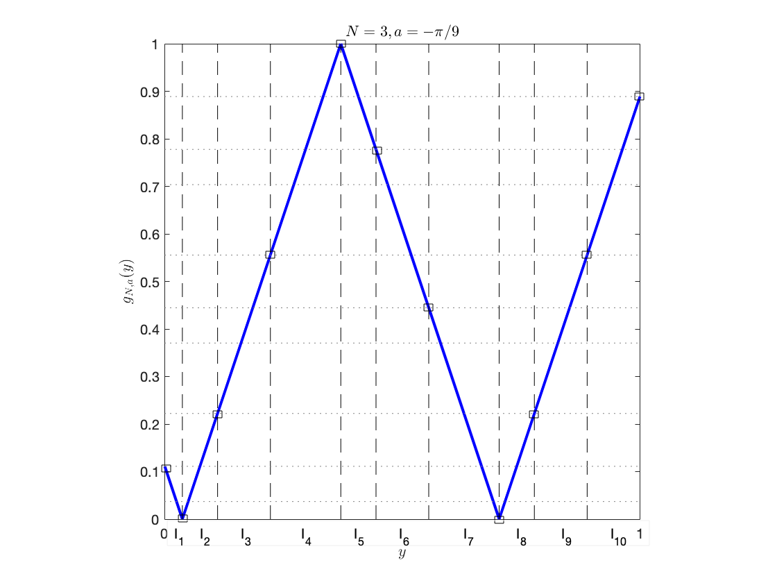
Appendix B An example of a non-trivial invariant density for a piecewise-linear map gN,asubscript𝑔𝑁𝑎g_{N,a}: N=3,a=π9formulae-sequence𝑁3𝑎𝜋9N=3,a=-\frac{\pi}{9}

A Markov partition is defined such that the slope is constant on each subinterval and boundary points map to boundary points. For g3,π9subscript𝑔3𝜋9g_{3,-\frac{\pi}{9}} such a partition, given by the eleven edge points of the partition indicated in Fig.15, consists of ten subintervals I=[0,1]=i=110Ii𝐼01superscriptsubscript𝑖110subscript𝐼𝑖I=[0,1]=\cup_{i=1}^{10}I_{i}.

Refer to caption
(a)
Figure 15: Markov partition of the piecewise-linear map g3,π/9(y)subscript𝑔3𝜋9𝑦g_{3,-\pi/9}(y) with partition points y=0,127,19,29,1027,49,59,1927,79,89,1𝑦0127192910274959192779891y=0,\frac{1}{27},\frac{1}{9},\frac{2}{9},\frac{10}{27},\frac{4}{9},\frac{5}{9},\frac{19}{27},\frac{7}{9},\frac{8}{9},1, indicated by dashed vertical lines.

We have g(I1)=I1I2𝑔subscript𝐼1subscript𝐼1subscript𝐼2g(I_{1})=I_{1}\cup I_{2}, g(I2)=I1I2I3𝑔subscript𝐼2subscript𝐼1subscript𝐼2subscript𝐼3g(I_{2})=I_{1}\cup I_{2}\cup I_{3}, g(I3)=I4I5I6𝑔subscript𝐼3subscript𝐼4subscript𝐼5subscript𝐼6g(I_{3})=I_{4}\cup I_{5}\cup I_{6}, etc. The transition matrix A𝐴A is therefore

A=(1100000000111000000000011100000000001111000000001100000111001111100000111000000000011100000000001110).𝐴matrix1100000000111000000000011100000000001111000000001100000111001111100000111000000000011100000000001110A=\begin{pmatrix}1&1&0&0&0&0&0&0&0&0\\ 1&1&1&0&0&0&0&0&0&0\\ 0&0&0&1&1&1&0&0&0&0\\ 0&0&0&0&0&0&1&1&1&1\\ 0&0&0&0&0&0&0&0&1&1\\ 0&0&0&0&0&1&1&1&0&0\\ 1&1&1&1&1&0&0&0&0&0\\ 1&1&1&0&0&0&0&0&0&0\\ 0&0&0&1&1&1&0&0&0&0\\ 0&0&0&0&0&0&1&1&1&0\end{pmatrix}.

The invariant density ρ𝜌\rho is determined by the (right-)eigenvector of the transfer matrix B=13At𝐵13superscript𝐴𝑡B=\frac{1}{3}A^{t} (t𝑡t denotes transpose) associated with the unit eigenvalue: ρ=Bρ𝜌𝐵𝜌\rho=B\rho,

ρ={α1α2=α1α3=23α1α4=2138α1α5=2138α1α6=3357α1α7=12α1α8=12α1α9=2857α1α10=719α1𝜌casessubscript𝛼1otherwisesubscript𝛼2subscript𝛼1otherwisesubscript𝛼323subscript𝛼1otherwisesubscript𝛼42138subscript𝛼1otherwisesubscript𝛼52138subscript𝛼1otherwisesubscript𝛼63357subscript𝛼1otherwisesubscript𝛼712subscript𝛼1otherwisesubscript𝛼812subscript𝛼1otherwisesubscript𝛼92857subscript𝛼1otherwisesubscript𝛼10719subscript𝛼1otherwise\rho=\begin{cases}\alpha_{1}\\ \alpha_{2}=\alpha_{1}\\ \alpha_{3}=\frac{2}{3}\alpha_{1}\\ \alpha_{4}=\frac{21}{38}\alpha_{1}\\ \alpha_{5}=\frac{21}{38}\alpha_{1}\\ \alpha_{6}=\frac{33}{57}\alpha_{1}\\ \alpha_{7}=\frac{1}{2}\alpha_{1}\\ \alpha_{8}=\frac{1}{2}\alpha_{1}\\ \alpha_{9}=\frac{28}{57}\alpha_{1}\\ \alpha_{10}=\frac{7}{19}\alpha_{1}\end{cases}

Using the normalisation condition 1=i=110αi1superscriptsubscript𝑖110subscript𝛼𝑖1=\sum_{i=1}^{10}\alpha_{i} we get α1=19118subscript𝛼119118\alpha_{1}=\frac{19}{118}. Hence, the invariant density of g3,π9subscript𝑔3𝜋9g_{3,-\frac{\pi}{9}} is

ρ(y)={191180.161,y[0,19)191770.107,y[19,29)212360.089,y[29,49)111180.093,y[49,59)192360.081,y[59,79)141770.079,y[79,89)71180.059,y[89,1]𝜌𝑦cases191180.161𝑦019191770.107𝑦1929212360.089𝑦2949111180.093𝑦4959192360.081𝑦5979141770.079𝑦798971180.059𝑦891\rho(y)=\begin{cases}\frac{19}{118}\approx 0.161,&y\in\left[0,\frac{1}{9}\right)\\ \frac{19}{177}\approx 0.107,&y\in\left[\frac{1}{9},\frac{2}{9}\right)\\ \frac{21}{236}\approx 0.089,&y\in\left[\frac{2}{9},\frac{4}{9}\right)\\ \frac{11}{118}\approx 0.093,&y\in\left[\frac{4}{9},\frac{5}{9}\right)\\ \frac{19}{236}\approx 0.081,&y\in\left[\frac{5}{9},\frac{7}{9}\right)\\ \frac{14}{177}\approx 0.079,&y\in\left[\frac{7}{9},\frac{8}{9}\right)\\ \frac{7}{118}\approx 0.059,&y\in\left[\frac{8}{9},1\right]\end{cases} (8)

which coincides with the numerical result in Fig.3h.

Appendix C Proof of eigenfunctions of the PF operator for multi-upside-down tent and multi-tent maps

(i) For multi-upside-down tent maps, gNsubscript𝑔𝑁g_{N} with even N𝑁N, the general piecewise-linear map gNsubscript𝑔𝑁g_{N} illustrated in Fig.4a is defined explicitly as

gN(x)={1Nx,x[0,1N]Nx1,x[1N,2N]3Nx,x[2N,3N]2k+1Nx,x[2kN,2k+1N]Nx(2k+1),x[2k+1N,2k+2N]Nx(N1),x[N1N,1].subscript𝑔𝑁𝑥cases1𝑁𝑥𝑥01𝑁otherwise𝑁𝑥1𝑥1𝑁2𝑁otherwise3𝑁𝑥𝑥2𝑁3𝑁otherwiseotherwise2𝑘1𝑁𝑥𝑥2𝑘𝑁2𝑘1𝑁otherwise𝑁𝑥2𝑘1𝑥2𝑘1𝑁2𝑘2𝑁otherwiseotherwise𝑁𝑥𝑁1𝑥𝑁1𝑁1otherwiseg_{N}(x)=\begin{cases}1-Nx,\quad x\in[0,\frac{1}{N}]\\ Nx-1,\quad x\in[\frac{1}{N},\frac{2}{N}]\\ 3-Nx,\quad x\in[\frac{2}{N},\frac{3}{N}]\\ \vdots\\ 2k+1-Nx,\quad x\in[\frac{2k}{N},\frac{2k+1}{N}]\\ Nx-(2k+1),\quad x\in[\frac{2k+1}{N},\frac{2k+2}{N}]\\ \vdots\\ Nx-(N-1),\quad x\in[\frac{N-1}{N},1]\end{cases}.

From definition of the PF operator \mathcal{L} we have

ρ(y)=xgN1(y)ρ(x)|gN(x)|=1N(ρ(x1)+ρ(x2)++ρ(xN)),𝜌𝑦subscript𝑥superscriptsubscript𝑔𝑁1𝑦𝜌𝑥subscriptsuperscript𝑔𝑁𝑥1𝑁𝜌subscript𝑥1𝜌subscript𝑥2𝜌subscript𝑥𝑁\mathcal{L}\rho(y)=\sum_{x\in g_{N}^{-1}(y)}\frac{\rho(x)}{|g^{\prime}_{N}(x)|}=\frac{1}{N}(\rho(x_{1})+\rho(x_{2})+...+\rho(x_{N})),

where xisubscript𝑥𝑖x_{i} (i=1,,N𝑖1𝑁i=1,...,N) are the preimages of y[0,1]𝑦01y\in[0,1] under the map gNsubscript𝑔𝑁g_{N}. Assuming the eigenvalues are λ(n)=N2nsuperscript𝜆𝑛superscript𝑁2𝑛\lambda^{(n)}=N^{-2n}, then the eigenvalue equation ρ(n)(y)=λ(n)ρ(n)(y)superscript𝜌𝑛𝑦superscript𝜆𝑛superscript𝜌𝑛𝑦\mathcal{L}\rho^{(n)}(y)=\lambda^{(n)}\rho^{(n)}(y) gives

1N(ρ(n)(x1)+ρ(n)(x2)++ρ(n)(xN))=N2nρ(n)(y),1𝑁superscript𝜌𝑛subscript𝑥1superscript𝜌𝑛subscript𝑥2superscript𝜌𝑛subscript𝑥𝑁superscript𝑁2𝑛superscript𝜌𝑛𝑦\frac{1}{N}(\rho^{(n)}(x_{1})+\rho^{(n)}(x_{2})+...+\rho^{(n)}(x_{N}))=N^{-2n}\rho^{(n)}(y),

or explicitly

N2n1[ρ(n)(1yN)+ρ(n)(1+yN)++ρ(n)(y+(N1)N)]=ρ(n)(y),superscript𝑁2𝑛1delimited-[]superscript𝜌𝑛1𝑦𝑁superscript𝜌𝑛1𝑦𝑁superscript𝜌𝑛𝑦𝑁1𝑁superscript𝜌𝑛𝑦N^{2n-1}\left[\rho^{(n)}\left(\frac{1-y}{N}\right)+\rho^{(n)}\left(\frac{1+y}{N}\right)+...+\rho^{(n)}\left(\frac{y+(N-1)}{N}\right)\right]=\rho^{(n)}(y), (9)

for n0𝑛subscript0n\in\mathbb{N}_{0}.
Claim 1: ρ(n)(x)=B2n(x2+12)superscript𝜌𝑛𝑥subscript𝐵2𝑛𝑥212\rho^{(n)}(x)=B_{2n}(\frac{x}{2}+\frac{1}{2}), where Bn(x)subscript𝐵𝑛𝑥B_{n}(x) are the Bernoulli polynomials.

Proof.

Using the Multiplication Theorem for Bnsubscript𝐵𝑛B_{n} with n=2n,m=Nformulae-sequence𝑛2𝑛𝑚𝑁n=2n,m=N (even) and x=1N(x2+12)𝑥1𝑁𝑥212x=\frac{1}{N}\left(\frac{x}{2}+\frac{1}{2}\right) we have

B2n(x2+12)=B2n(Nx+12N)=N2n1k=0N1B2n(x+12N+kN)=N2n1[B2n(x2N+12N)+B2n(x2N+32N)++B2n(x2N+2N12N)].subscript𝐵2𝑛𝑥212subscript𝐵2𝑛𝑁𝑥12𝑁superscript𝑁2𝑛1superscriptsubscript𝑘0𝑁1subscript𝐵2𝑛𝑥12𝑁𝑘𝑁superscript𝑁2𝑛1delimited-[]subscript𝐵2𝑛𝑥2𝑁12𝑁subscript𝐵2𝑛𝑥2𝑁32𝑁subscript𝐵2𝑛𝑥2𝑁2𝑁12𝑁\begin{split}B_{2n}\left(\frac{x}{2}+\frac{1}{2}\right)&=B_{2n}\left(N\cdot\frac{x+1}{2N}\right)\\ &=N^{2n-1}\sum_{k=0}^{N-1}B_{2n}\left(\frac{x+1}{2N}+\frac{k}{N}\right)\\ &=N^{2n-1}\left[B_{2n}\left(\frac{x}{2N}+\frac{1}{2N}\right)+B_{2n}\left(\frac{x}{2N}+\frac{3}{2N}\right)+...+B_{2n}\left(\frac{x}{2N}+\frac{2N-1}{2N}\right)\right].\end{split} (10)

Now we want to show that each term in the last expression corresponds to a term in LHS of (9).

If Claim 1 is true, we have

ρ(n)(x1)=ρ(n)(1yN)=B2n(121yN+12)=B2n(121y2N)=B2n(y2N+N12N),superscript𝜌𝑛subscript𝑥1superscript𝜌𝑛1𝑦𝑁subscript𝐵2𝑛121𝑦𝑁12subscript𝐵2𝑛121𝑦2𝑁subscript𝐵2𝑛𝑦2𝑁𝑁12𝑁\rho^{(n)}(x_{1})=\rho^{(n)}\left(\frac{1-y}{N}\right)=B_{2n}\left(\frac{1}{2}\cdot\frac{1-y}{N}+\frac{1}{2}\right)=B_{2n}\left(\frac{1}{2}-\frac{1-y}{2N}\right)=B_{2n}\left(\frac{y}{2N}+\frac{N-1}{2N}\right),

where in the second equality we have used a symmetry property of B2nsubscript𝐵2𝑛B_{2n} (basically whenever there is a minus sign in front of a term involving y𝑦y we need to use this symmetry), and also

ρ(n)(x2)=ρ(n)(1+yN)=B2n(121+yN+12)=B2n(y2N+N+12N).superscript𝜌𝑛subscript𝑥2superscript𝜌𝑛1𝑦𝑁subscript𝐵2𝑛121𝑦𝑁12subscript𝐵2𝑛𝑦2𝑁𝑁12𝑁\rho^{(n)}(x_{2})=\rho^{(n)}\left(\frac{1+y}{N}\right)=B_{2n}\left(\frac{1}{2}\cdot\frac{1+y}{N}+\frac{1}{2}\right)=B_{2n}\left(\frac{y}{2N}+\frac{N+1}{2N}\right).

By induction, we have

ρ(n)(x2k1)=ρ(n)((2k1)yN)=B2n(y2N+N+(2k1)2N),ρ(n)(x2k)=ρ(n)(2kyN)=B2n(y2N+N(2k1)2N),formulae-sequencesuperscript𝜌𝑛subscript𝑥2𝑘1superscript𝜌𝑛2𝑘1𝑦𝑁subscript𝐵2𝑛𝑦2𝑁𝑁2𝑘12𝑁superscript𝜌𝑛subscript𝑥2𝑘superscript𝜌𝑛2𝑘𝑦𝑁subscript𝐵2𝑛𝑦2𝑁𝑁2𝑘12𝑁\begin{split}\rho^{(n)}(x_{2k-1})&=\rho^{(n)}\left(\frac{(2k-1)-y}{N}\right)=B_{2n}\left(\frac{y}{2N}+\frac{N+(2k-1)}{2N}\right),\\ \rho^{(n)}(x_{2k})&=\rho^{(n)}\left(\frac{2k-y}{N}\right)=B_{2n}\left(\frac{y}{2N}+\frac{N-(2k-1)}{2N}\right),\end{split}

for all integers 1kN21𝑘𝑁21\leq k\leq\frac{N}{2}. So the last two preimages xN1subscript𝑥𝑁1x_{N-1} and xNsubscript𝑥𝑁x_{N} correspond to

ρ(n)(xN1)=ρ(n)((N1)yN)=B2n(y2N+2N12N),ρ(n)(xN)=ρ(n)(NyN)=B2n(y2N+12N),formulae-sequencesuperscript𝜌𝑛subscript𝑥𝑁1superscript𝜌𝑛𝑁1𝑦𝑁subscript𝐵2𝑛𝑦2𝑁2𝑁12𝑁superscript𝜌𝑛subscript𝑥𝑁superscript𝜌𝑛𝑁𝑦𝑁subscript𝐵2𝑛𝑦2𝑁12𝑁\begin{split}\rho^{(n)}(x_{N-1})&=\rho^{(n)}\left(\frac{(N-1)-y}{N}\right)=B_{2n}\left(\frac{y}{2N}+\frac{2N-1}{2N}\right),\\ \rho^{(n)}(x_{N})&=\rho^{(n)}\left(\frac{N-y}{N}\right)=B_{2n}\left(\frac{y}{2N}+\frac{1}{2N}\right),\end{split}

for which reason we group pairs of consecutive preimages together in Fig.4a. Therefore, (9) and (10) are equivalent, and Claim 1 together with the eigenvalue assumption hold.

(ii) For multi-tent maps (cf. Fig.4b), similarly, the piecewise-linear map is defined as

gN(x)={Nx,x[0,1N]2Nx,x[1N,2N]Nx2,x[2N,3N]Nx2k,x[2kN,2k+1N]2k+2Nx,x[2k+1N,2k+2N]Nx(N1),x[N1N,1].subscript𝑔𝑁𝑥cases𝑁𝑥𝑥01𝑁otherwise2𝑁𝑥𝑥1𝑁2𝑁otherwise𝑁𝑥2𝑥2𝑁3𝑁otherwiseotherwise𝑁𝑥2𝑘𝑥2𝑘𝑁2𝑘1𝑁otherwise2𝑘2𝑁𝑥𝑥2𝑘1𝑁2𝑘2𝑁otherwiseotherwise𝑁𝑥𝑁1𝑥𝑁1𝑁1otherwiseg_{N}(x)=\begin{cases}Nx,\quad x\in[0,\frac{1}{N}]\\ 2-Nx,\quad x\in[\frac{1}{N},\frac{2}{N}]\\ Nx-2,\quad x\in[\frac{2}{N},\frac{3}{N}]\\ \vdots\\ Nx-2k,\quad x\in[\frac{2k}{N},\frac{2k+1}{N}]\\ 2k+2-Nx,\quad x\in[\frac{2k+1}{N},\frac{2k+2}{N}]\\ \vdots\\ Nx-(N-1),\quad x\in[\frac{N-1}{N},1]\end{cases}.

Again, by definition of the transfer operator \mathcal{L} and eigenvalue equation, assuming λ(n)=N2nsuperscript𝜆𝑛superscript𝑁2𝑛\lambda^{(n)}=N^{-2n}, we get

N2n1[ρ(n)(yN)+ρ(n)(2yN)++ρ(n)(yN+N1N)]=ρ(n)(y),superscript𝑁2𝑛1delimited-[]superscript𝜌𝑛𝑦𝑁superscript𝜌𝑛2𝑦𝑁superscript𝜌𝑛𝑦𝑁𝑁1𝑁superscript𝜌𝑛𝑦N^{2n-1}\left[\rho^{(n)}\left(\frac{y}{N}\right)+\rho^{(n)}\left(\frac{2-y}{N}\right)+...+\rho^{(n)}\left(\frac{y}{N}+\frac{N-1}{N}\right)\right]=\rho^{(n)}(y), (11)

for n0𝑛subscript0n\in\mathbb{N}_{0}.
Claim 2a: ρ(n)(x)=B2n(x)superscript𝜌𝑛𝑥subscript𝐵2𝑛𝑥\rho^{(n)}(x)=B_{2n}(x), where Bn(x)subscript𝐵𝑛𝑥B_{n}(x) are the Bernoulli polynomials.

Proof.

By the Multiplication Theorem for Bnsubscript𝐵𝑛B_{n} with n=2n,m=Nformulae-sequence𝑛2𝑛𝑚𝑁n=2n,m=N (odd) and x=xN𝑥𝑥𝑁x=\frac{x}{N} we have

B2n(x)=B2n(NxN)=N2n1k=0N1B2n(xN+kN)=N2n1[B2n(xN)+B2n(xN+1N)++B2n(xN+N1N)].subscript𝐵2𝑛𝑥subscript𝐵2𝑛𝑁𝑥𝑁superscript𝑁2𝑛1superscriptsubscript𝑘0𝑁1subscript𝐵2𝑛𝑥𝑁𝑘𝑁superscript𝑁2𝑛1delimited-[]subscript𝐵2𝑛𝑥𝑁subscript𝐵2𝑛𝑥𝑁1𝑁subscript𝐵2𝑛𝑥𝑁𝑁1𝑁\begin{split}B_{2n}(x)&=B_{2n}\left(N\cdot\frac{x}{N}\right)\\ &=N^{2n-1}\sum_{k=0}^{N-1}B_{2n}\left(\frac{x}{N}+\frac{k}{N}\right)\\ &=N^{2n-1}\left[B_{2n}\left(\frac{x}{N}\right)+B_{2n}\left(\frac{x}{N}+\frac{1}{N}\right)+...+B_{2n}\left(\frac{x}{N}+\frac{N-1}{N}\right)\right].\end{split}

This expression is equivalent to (11) since there is a term-to-term correspondence 222This is a re-ordering the N𝑁N (odd) preimages {x1,x2,,xN}subscript𝑥1subscript𝑥2subscript𝑥𝑁\{x_{1},x_{2},...,x_{N}\} in the way that
i) if N=4q+1𝑁4𝑞1N=4q+1, the index of the middle point of natural ordering is odd then
x1xN1x3xN3x5xN5xN+12+1xN+12xN+121xN+12+2xN+123xN+12+4xN+125x2xN;subscript𝑥1subscript𝑥𝑁1subscript𝑥3subscript𝑥𝑁3subscript𝑥5subscript𝑥𝑁5subscript𝑥𝑁121subscript𝑥𝑁12subscript𝑥𝑁121subscript𝑥𝑁122subscript𝑥𝑁123subscript𝑥𝑁124subscript𝑥𝑁125subscript𝑥2subscript𝑥𝑁\begin{split}x_{1}&\rightarrow x_{N-1}\rightarrow x_{3}\rightarrow x_{N-3}\rightarrow x_{5}\rightarrow x_{N-5}\rightarrow...\\ &\rightarrow x_{\frac{N+1}{2}+1}\rightarrow x_{\frac{N+1}{2}}\rightarrow x_{\frac{N+1}{2}-1}\rightarrow x_{\frac{N+1}{2}+2}\rightarrow x_{\frac{N+1}{2}-3}\rightarrow x_{\frac{N+1}{2}+4}\rightarrow x_{\frac{N+1}{2}-5}\rightarrow...\rightarrow x_{2}\rightarrow x_{N};\end{split} and ii) if N=4q1𝑁4𝑞1N=4q-1, the index of the middle point of natural ordering is even then x1xN1x3xN3x5xN5xN+121xN+12xN+12+1xN+122xN+12+3xN+124xN+12+5x2xN.subscript𝑥1subscript𝑥𝑁1subscript𝑥3subscript𝑥𝑁3subscript𝑥5subscript𝑥𝑁5subscript𝑥𝑁121subscript𝑥𝑁12subscript𝑥𝑁121subscript𝑥𝑁122subscript𝑥𝑁123subscript𝑥𝑁124subscript𝑥𝑁125subscript𝑥2subscript𝑥𝑁\begin{split}x_{1}&\rightarrow x_{N-1}\rightarrow x_{3}\rightarrow x_{N-3}\rightarrow x_{5}\rightarrow x_{N-5}\rightarrow...\\ &\rightarrow x_{\frac{N+1}{2}-1}\rightarrow x_{\frac{N+1}{2}}\rightarrow x_{\frac{N+1}{2}+1}\rightarrow x_{\frac{N+1}{2}-2}\rightarrow x_{\frac{N+1}{2}+3}\rightarrow x_{\frac{N+1}{2}-4}\rightarrow x_{\frac{N+1}{2}+5}\rightarrow...\rightarrow x_{2}\rightarrow x_{N}.\end{split}
Compare to the even N𝑁N case, where the re-ordering reads
xNxN2xN4x4x2x1x3x5xN3xN1.subscript𝑥𝑁subscript𝑥𝑁2subscript𝑥𝑁4subscript𝑥4subscript𝑥2subscript𝑥1subscript𝑥3subscript𝑥5subscript𝑥𝑁3subscript𝑥𝑁1x_{N}\rightarrow x_{N-2}\rightarrow x_{N-4}\rightarrow...\rightarrow x_{4}\rightarrow x_{2}\rightarrow x_{1}\rightarrow x_{3}\rightarrow x_{5}\rightarrow...\rightarrow x_{N-3}\rightarrow x_{N-1}.

ρ(n)(x2k1)=ρ(n)(yN+2k2N)=B2n(yN+2k2N),ρ(n)(x2k)=ρ(n)(2kNyN)=B2n(2kNyN)=B2n(12(yN+122kN))=B2n(12+(yN+122kN))=B2n(yN+N2kN),formulae-sequencesuperscript𝜌𝑛subscript𝑥2𝑘1superscript𝜌𝑛𝑦𝑁2𝑘2𝑁subscript𝐵2𝑛𝑦𝑁2𝑘2𝑁superscript𝜌𝑛subscript𝑥2𝑘superscript𝜌𝑛2𝑘𝑁𝑦𝑁subscript𝐵2𝑛2𝑘𝑁𝑦𝑁subscript𝐵2𝑛12𝑦𝑁122𝑘𝑁subscript𝐵2𝑛12𝑦𝑁122𝑘𝑁subscript𝐵2𝑛𝑦𝑁𝑁2𝑘𝑁\begin{split}\rho^{(n)}(x_{2k-1})&=\rho^{(n)}\left(\frac{y}{N}+\frac{2k-2}{N}\right)=B_{2n}\left(\frac{y}{N}+\frac{2k-2}{N}\right),\\ \rho^{(n)}(x_{2k})&=\rho^{(n)}\left(\frac{2k}{N}-\frac{y}{N}\right)=B_{2n}\left(\frac{2k}{N}-\frac{y}{N}\right)=B_{2n}\left(\frac{1}{2}-(\frac{y}{N}+\frac{1}{2}-\frac{2k}{N})\right)\\ &\quad=B_{2n}\left(\frac{1}{2}+(\frac{y}{N}+\frac{1}{2}-\frac{2k}{N})\right)=B_{2n}\left(\frac{y}{N}+\frac{N-2k}{N}\right),\end{split}

for all integers 1kN121𝑘𝑁121\leq k\leq\frac{N-1}{2}, for which one can easily verify that

ρ(n)(x1)=B2n(yN),ρ(n)(x2)=B2n(yN+N2N),formulae-sequencesuperscript𝜌𝑛subscript𝑥1subscript𝐵2𝑛𝑦𝑁superscript𝜌𝑛subscript𝑥2subscript𝐵2𝑛𝑦𝑁𝑁2𝑁\begin{split}\rho^{(n)}(x_{1})&=B_{2n}\left(\frac{y}{N}\right),\\ \rho^{(n)}(x_{2})&=B_{2n}\left(\frac{y}{N}+\frac{N-2}{N}\right),\end{split}

and

ρ(n)(xN1)=B2n(yN+1N),ρ(n)(xN)=B2n(yN+N1N).formulae-sequencesuperscript𝜌𝑛subscript𝑥𝑁1subscript𝐵2𝑛𝑦𝑁1𝑁superscript𝜌𝑛subscript𝑥𝑁subscript𝐵2𝑛𝑦𝑁𝑁1𝑁\begin{split}\rho^{(n)}(x_{N-1})&=B_{2n}\left(\frac{y}{N}+\frac{1}{N}\right),\\ \rho^{(n)}(x_{N})&=B_{2n}\left(\frac{y}{N}+\frac{N-1}{N}\right).\end{split}

Hence the Claim 2a.

Claim 2b: ρ(n)(x)=E2n1(x)superscript𝜌𝑛𝑥subscript𝐸2𝑛1𝑥\rho^{(n)}(x)=E_{2n-1}(x), where En(x)subscript𝐸𝑛𝑥E_{n}(x) are the Euler polynomials.

Proof.

Indeed it can be verified that E2n1(x)subscript𝐸2𝑛1𝑥E_{2n-1}(x) is also an eigenfunction for the multi-tent map gN(x)subscript𝑔𝑁𝑥g_{N}(x) with N3𝑁3N\geq 3 odd, corresponding to the eigenvalue N2nsuperscript𝑁2𝑛N^{-2n}. The proof uses the Multiplication Theorem for Ensubscript𝐸𝑛E_{n}

En(mx)=mnk=0m1(1)kEn(x+km),m=1,3,,formulae-sequencesubscript𝐸𝑛𝑚𝑥superscript𝑚𝑛superscriptsubscript𝑘0𝑚1superscript1𝑘subscript𝐸𝑛𝑥𝑘𝑚𝑚13E_{n}(mx)=m^{n}\sum_{k=0}^{m-1}(-1)^{k}E_{n}\left(x+\frac{k}{m}\right),\quad m=1,3,...,

with k=N𝑘𝑁k=N (odd), x=xN𝑥𝑥𝑁x=\frac{x}{N} and m=2n1𝑚2𝑛1m=2n-1, and an anti-symmetry property for odd Euler polynomials: E2n1(12x)=E2n1(12+x)subscript𝐸2𝑛112𝑥subscript𝐸2𝑛112𝑥E_{2n-1}\left(\frac{1}{2}-x\right)=-E_{2n-1}\left(\frac{1}{2}+x\right). This indicates a degeneracy for odd N𝑁N multi-tent maps gN(x)subscript𝑔𝑁𝑥g_{N}(x), therefore also for odd Chebyshev maps TN,0(x)subscript𝑇𝑁0𝑥T_{N,0}(x). ∎

Appendix D Discussion of eigenfunctions for odd-N𝑁N shifted Chebyshev maps

In this case, a more complicated situation arises from the fact that, when a0𝑎0a\neq 0, for an arbitrary x[0,1]𝑥01x\in[0,1] the piecewise-linear map gN,asubscript𝑔𝑁𝑎g_{N,a} can have different numbers of preimages, for example, for g3,asubscript𝑔3𝑎g_{3,a} (cf. Fig.2b), there can be 1, 2, 3 or 4 preimages that separate the unit interval into several subintervals, and we need to take into account the values of x𝑥x in each of the subintervals, resulting in the eigenfunctions being piecewise defined. This is consistent with the fact from section 2.3 that the invariant densities for some TN,asubscript𝑇𝑁𝑎T_{N,a} are not always smooth but piecewise smooth (cf. last three columns in Fig.3).

We therefore conjecture that in the case of a=πm𝑎𝜋𝑚a=-\frac{\pi}{m} (m=2,3,𝑚23m=2,3,...), eigenfunctions of the PF operator for TN,asubscript𝑇𝑁𝑎T_{N,a} are of the form

ρTN,a(n)(x)=k=1mNnαn,kχIn,k(x)1π1x2Fn(x),x[1,1],formulae-sequencesubscriptsuperscript𝜌𝑛subscript𝑇𝑁𝑎𝑥superscriptsubscript𝑘1𝑚superscript𝑁𝑛subscript𝛼𝑛𝑘subscript𝜒subscript𝐼𝑛𝑘𝑥1𝜋1superscript𝑥2subscript𝐹𝑛𝑥𝑥11\rho^{(n)}_{T_{N,a}}(x)=\sum_{k=1}^{mN^{n}}\alpha_{n,k}\chi_{I_{n,k}}(x)\frac{1}{\pi\sqrt{1-x^{2}}}F_{n}(x),\quad x\in[-1,1], (12)

where αn,k=αn,k(λ(n))subscript𝛼𝑛𝑘subscript𝛼𝑛𝑘superscript𝜆𝑛\alpha_{n,k}=\alpha_{n,k}(\lambda^{(n)}) are the weights depending on the associated eigenvalue 0<λ(n)10superscript𝜆𝑛10<\lambda^{(n)}\leq 1, χI(x)subscript𝜒𝐼𝑥\chi_{I}(x) is the indicator function such that χI(x)=1subscript𝜒𝐼𝑥1\chi_{I}(x)=1 if xI𝑥𝐼x\in I and 00 otherwise. The partition In,k=[k1mNn,kmNn)subscript𝐼𝑛𝑘𝑘1𝑚superscript𝑁𝑛𝑘𝑚superscript𝑁𝑛I_{n,k}=\left[\frac{k-1}{mN^{n}},\frac{k}{mN^{n}}\right) may vary according to the order n𝑛n of the eigenvalue; the last subinterval includes the right-boundary point 1, In,mNn=[mNn1mNn,1]subscript𝐼𝑛𝑚superscript𝑁𝑛𝑚superscript𝑁𝑛1𝑚superscript𝑁𝑛1I_{n,mN^{n}}=\left[\frac{mN^{n}-1}{mN^{n}},1\right], so that In,k1In,k2=,k1k2formulae-sequencesubscript𝐼𝑛subscript𝑘1subscript𝐼𝑛subscript𝑘2for-allsubscript𝑘1subscript𝑘2I_{n,k_{1}}\cap I_{n,k_{2}}=\emptyset,\forall k_{1}\neq k_{2} and kIn,k=I=[0,1]subscript𝑘subscript𝐼𝑛𝑘𝐼01\cup_{k}I_{n,k}=I=[0,1] for any given n0𝑛subscript0n\in\mathbb{N}_{0}. This forms a hierarchically finer structure in partitioning the unit interval, initially defined by the Markov partition at the invariant density level (n=0𝑛0n=0, with λ(0)=1superscript𝜆01\lambda^{(0)}=1 being the largest eigenvalue). {Fn}subscript𝐹𝑛\{F_{n}\} are some appropriate smooth functions with F0(x)=1subscript𝐹0𝑥1F_{0}(x)=1 x[1,1]for-all𝑥11\forall x\in[-1,1].

In particular, similarly to eq.(3), we have

(T2m,0)TN,πm=TN,0(T2m,0)=T2mN,0,N odd,formulae-sequencesubscript𝑇2𝑚0subscript𝑇𝑁𝜋𝑚subscript𝑇𝑁0subscript𝑇2𝑚0subscript𝑇2𝑚𝑁0𝑁 odd(-T_{2m,0})\circ T_{N,-\frac{\pi}{m}}=T_{N,0}\circ(-T_{2m,0})=-T_{2mN,0},\quad N\text{ odd}, (13)

that is, the odd N𝑁N shifted Chebyshev map TN,πmsubscript𝑇𝑁𝜋𝑚T_{N,-\frac{\pi}{m}} is topologically semi-conjugated to its corresponding ordinary TN,0subscript𝑇𝑁0T_{N,0} via the semi-conjugacy h2(x):=T2m,0(x)assignsubscript2𝑥subscript𝑇2𝑚0𝑥h_{2}(x):=-T_{2m,0}(x), m2𝑚subscriptabsent2m\in\mathbb{N}_{\geq 2}. By a coordinate transformation one gets the shape of eigenfunctions for TN,πmsubscript𝑇𝑁𝜋𝑚T_{N,-\frac{\pi}{m}} (N𝑁N odd) as (cf. eq.(2))

|h2(x)|ρTN,0(n)(h2(x))1π1x2B2n(2mπarccosx)or 1π1x2E2n1(2mπarccosx).proportional-tosuperscriptsubscript2𝑥superscriptsubscript𝜌subscript𝑇𝑁0𝑛subscript2𝑥1𝜋1superscript𝑥2subscript𝐵2𝑛2𝑚𝜋𝑥or proportional-to1𝜋1superscript𝑥2subscript𝐸2𝑛12𝑚𝜋𝑥\begin{split}|h_{2}^{\prime}(x)|\rho_{T_{N,0}}^{(n)}(h_{2}(x))\propto&\frac{1}{\pi\sqrt{1-x^{2}}}B_{2n}\left(\frac{2m}{\pi}\arccos x\right)\\ \text{or }\propto&\frac{1}{\pi\sqrt{1-x^{2}}}E_{2n-1}\left(\frac{2m}{\pi}\arccos x\right).\end{split}

So the set of smooth functions {Fn}subscript𝐹𝑛\{F_{n}\} in (12) can be chosen to be Bernoulli or Euler polynomials, and the eigenvalues λ(n)=N2nsuperscript𝜆𝑛superscript𝑁2𝑛\lambda^{(n)}=N^{-2n} remain the same.

Appendix E Derivation of higher-order correlations of iterates of shifted Chebyshev maps

Let xisubscript𝑥𝑖x_{i} be the i𝑖i-th iterate of a shifted Chebyshev map TN,0subscript𝑇𝑁0T_{N,0}. Using the change of variables described in Sec.2,

x0=cos(πu),xn=cos(Nnπu+Nn1N1a),formulae-sequencesubscript𝑥0𝜋𝑢subscript𝑥𝑛superscript𝑁𝑛𝜋𝑢superscript𝑁𝑛1𝑁1𝑎\begin{split}x_{0}&=\cos(\pi u),\\ x_{n}&=\cos\left(N^{n}\pi u+\frac{N^{n}-1}{N-1}a\right),\end{split}

we have, for shifted Chebyshev maps T𝑇T in the category (\star2.3),

xn1xnr=111π1cos2πucos(Nn1πu+Nn11N1a)cos(Nnrπu+Nnr1N1a)d(cosπu)=101πsinπucos(Nn1πu+Nn11N1a)cos(Nnrπu+Nnr1N1a)(πsinπu)𝑑u=01cos(Nn1πu+Nn11N1a)cos(Nnrπu+Nnr1N1a)𝑑u=01exp(i(Nn1πu+Nn11N1a))+exp(i(Nn1πu+Nn11N1a))2exp(i(Nnrπu+Nnr1N1a))+exp(i(Nnrπu+Nnr1N1a))2du=2rσ01exp(il=1rσl(Nnlπu+Nnl1N1a))𝑑u=2rσ[exp(ial=1rσlNnl1N1)01exp(iπul=1rσlNnl)𝑑u]=2rσ[exp(ial=1rσlNnl1N1)δ(l=1rσlNnl,0)],delimited-⟨⟩subscript𝑥subscript𝑛1subscript𝑥subscript𝑛𝑟superscriptsubscript111𝜋1superscript2𝜋𝑢superscript𝑁subscript𝑛1𝜋𝑢superscript𝑁subscript𝑛11𝑁1𝑎superscript𝑁subscript𝑛𝑟𝜋𝑢superscript𝑁subscript𝑛𝑟1𝑁1𝑎𝑑𝜋𝑢superscriptsubscript101𝜋𝜋𝑢superscript𝑁subscript𝑛1𝜋𝑢superscript𝑁subscript𝑛11𝑁1𝑎superscript𝑁subscript𝑛𝑟𝜋𝑢superscript𝑁subscript𝑛𝑟1𝑁1𝑎𝜋𝜋𝑢differential-d𝑢superscriptsubscript01superscript𝑁subscript𝑛1𝜋𝑢superscript𝑁subscript𝑛11𝑁1𝑎superscript𝑁subscript𝑛𝑟𝜋𝑢superscript𝑁subscript𝑛𝑟1𝑁1𝑎differential-d𝑢superscriptsubscript01𝑖superscript𝑁subscript𝑛1𝜋𝑢superscript𝑁subscript𝑛11𝑁1𝑎𝑖superscript𝑁subscript𝑛1𝜋𝑢superscript𝑁subscript𝑛11𝑁1𝑎2𝑖superscript𝑁subscript𝑛𝑟𝜋𝑢superscript𝑁subscript𝑛𝑟1𝑁1𝑎𝑖superscript𝑁subscript𝑛𝑟𝜋𝑢superscript𝑁subscript𝑛𝑟1𝑁1𝑎2𝑑𝑢superscript2𝑟subscript𝜎superscriptsubscript01𝑖superscriptsubscript𝑙1𝑟subscript𝜎𝑙superscript𝑁subscript𝑛𝑙𝜋𝑢superscript𝑁subscript𝑛𝑙1𝑁1𝑎differential-d𝑢superscript2𝑟subscript𝜎delimited-[]𝑖𝑎superscriptsubscript𝑙1𝑟subscript𝜎𝑙superscript𝑁subscript𝑛𝑙1𝑁1superscriptsubscript01𝑖𝜋𝑢superscriptsubscript𝑙1𝑟subscript𝜎𝑙superscript𝑁subscript𝑛𝑙differential-d𝑢superscript2𝑟subscript𝜎delimited-[]𝑖𝑎superscriptsubscript𝑙1𝑟subscript𝜎𝑙superscript𝑁subscript𝑛𝑙1𝑁1𝛿superscriptsubscript𝑙1𝑟subscript𝜎𝑙superscript𝑁subscript𝑛𝑙0\begin{split}\langle x_{n_{1}}\cdots x_{n_{r}}\rangle=&\int_{-1}^{1}\frac{1}{\pi\sqrt{1-\cos^{2}\pi u}}\cos\left(N^{n_{1}}\pi u+\frac{N^{n_{1}}-1}{N-1}a\right)\cdot...\cdot\cos\left(N^{n_{r}}\pi u+\frac{N^{n_{r}}-1}{N-1}a\right)d(\cos\pi u)\\ =&\int_{1}^{0}\frac{1}{\pi\sin\pi u}\cos\left(N^{n_{1}}\pi u+\frac{N^{n_{1}}-1}{N-1}a\right)\cdot...\cdot\cos\left(N^{n_{r}}\pi u+\frac{N^{n_{r}}-1}{N-1}a\right)\cdot(-\pi\sin\pi u)du\\ =&\int_{0}^{1}\cos\left(N^{n_{1}}\pi u+\frac{N^{n_{1}}-1}{N-1}a\right)\cdot...\cdot\cos\left(N^{n_{r}}\pi u+\frac{N^{n_{r}}-1}{N-1}a\right)du\\ =&\int_{0}^{1}\frac{\exp\left(i(N^{n_{1}}\pi u+\frac{N^{n_{1}}-1}{N-1}a)\right)+\exp\left(-i(N^{n_{1}}\pi u+\frac{N^{n_{1}}-1}{N-1}a)\right)}{2}\cdot...\\ &\quad\cdot\frac{\exp\left(i(N^{n_{r}}\pi u+\frac{N^{n_{r}}-1}{N-1}a)\right)+\exp\left(-i(N^{n_{r}}\pi u+\frac{N^{n_{r}}-1}{N-1}a)\right)}{2}du\\ =&2^{-r}\sum_{\sigma}\int_{0}^{1}\exp\left(i\sum_{l=1}^{r}\sigma_{l}\cdot\left(N^{n_{l}}\pi u+\frac{N^{n_{l}}-1}{N-1}a\right)\right)du\\ =&2^{-r}\sum_{\sigma}\left[\exp\left(ia\sum_{l=1}^{r}\sigma_{l}\frac{N^{n_{l}}-1}{N-1}\right)\cdot\int_{0}^{1}\exp\left(i\pi u\sum_{l=1}^{r}\sigma_{l}N^{n_{l}}\right)du\right]\\ =&2^{-r}\sum_{\sigma}\left[\exp\left(ia\sum_{l=1}^{r}\sigma_{l}\frac{N^{n_{l}}-1}{N-1}\right)\cdot\delta\left(\sum_{l=1}^{r}\sigma_{l}N^{n_{l}},0\right)\right],\end{split}

where in the fourth line we have used the Euler formula cosx=12(eix+eix)𝑥12superscript𝑒𝑖𝑥superscript𝑒𝑖𝑥\cos x=\frac{1}{2}(e^{ix}+e^{-ix}); in the fifth line σlsubscript𝜎𝑙\sigma_{l} denotes a choice of the spin configuration {1,+1}11\{-1,+1\} and the sum over σ𝜎\sigma is a summation over all possible configurations σ:=(σ1,σ2,,σr)assign𝜎subscript𝜎1subscript𝜎2subscript𝜎𝑟\sigma:=(\sigma_{1},\sigma_{2},...,\sigma_{r}), σl{1,+1}subscript𝜎𝑙11\sigma_{l}\in\{-1,+1\}; in the last line δ(x,0)𝛿𝑥0\delta(x,0) is the Kronecker delta defined as being 1 if x=0𝑥0x=0 and 0 else.

Appendix F Derivation of the two-point correlation function for the N𝑁N-ary shift with subtracted mean

Consider the N𝑁N-ary shift xn+1=f(xn)=Nxmod1subscript𝑥𝑛1𝑓subscript𝑥𝑛modulo𝑁𝑥1x_{n+1}=f(x_{n})=Nx\mod 1, x0[0,1]subscript𝑥001x_{0}\in[0,1], N2𝑁subscriptabsent2N\in\mathbb{N}_{\geq 2}.

With the N𝑁N-ary representation of the initial point x0=j=1ajNjsubscript𝑥0superscriptsubscript𝑗1subscript𝑎𝑗superscript𝑁𝑗x_{0}=\sum_{j=1}^{\infty}a_{j}N^{-j}, aj{0,1,,N1}subscript𝑎𝑗01𝑁1a_{j}\in\{0,1,...,N-1\} we have xn=j=1aj+nNjsubscript𝑥𝑛superscriptsubscript𝑗1subscript𝑎𝑗𝑛superscript𝑁𝑗x_{n}=\sum_{j=1}^{\infty}a_{j+n}N^{-j}.

Define

wn:=xnxn=j=1aj+nNj12=j=1aj+nNjN12j=1Nj=j=1bj+nNj,\begin{split}w_{n}:&=x_{n}-\langle x_{n}\rangle\\ &=\sum_{j=1}^{\infty}a_{j+n}N^{-j}-\frac{1}{2}\\ &=\sum_{j=1}^{\infty}a_{j+n}N^{-j}-\frac{N-1}{2}\sum_{j=1}^{\infty}N^{-j}\\ &=\sum_{j=1}^{\infty}b_{j+n}N^{-j},\end{split}

where bj+n{N12,N32,,N12}subscript𝑏𝑗𝑛𝑁12𝑁32𝑁12b_{j+n}\in\left\{-\frac{N-1}{2},-\frac{N-3}{2},...,\frac{N-1}{2}\right\} so that wnsubscript𝑤𝑛w_{n} has the average value zero.

Then

bj+nk=1N[(N12)k+(N32)k++(N32)k+(N12)k]={0,if k is odd2N[(N12)k+(N32)k++(NN+122)k],if k is even.delimited-⟨⟩superscriptsubscript𝑏𝑗𝑛𝑘1𝑁delimited-[]superscript𝑁12𝑘superscript𝑁32𝑘superscript𝑁32𝑘superscript𝑁12𝑘cases0if k is oddotherwise2𝑁delimited-[]superscript𝑁12𝑘superscript𝑁32𝑘superscript𝑁𝑁122𝑘if k is evenotherwise\begin{split}\langle b_{j+n}^{k}\rangle&=\frac{1}{N}\left[\left(-\frac{N-1}{2}\right)^{k}+\left(-\frac{N-3}{2}\right)^{k}+...+\left(\frac{N-3}{2}\right)^{k}+\left(\frac{N-1}{2}\right)^{k}\right]\\ &=\begin{cases}0,\quad\text{if $k$ is odd}\\ \frac{2}{N}\left[\left(\frac{N-1}{2}\right)^{k}+\left(\frac{N-3}{2}\right)^{k}+...+\left(\frac{N-\lceil\frac{N+1}{2}\rceil}{2}\right)^{k}\right],\quad\text{if $k$ is even}.\end{cases}\end{split}

Let us denote

SN,k:=(N12)k+(N32)k++(NN+122)k={12k(1+3k++(N1)k)if N is even1+2k++(N12)kif N is odd.\begin{split}S_{N,k}:&=\left(\frac{N-1}{2}\right)^{k}+\left(\frac{N-3}{2}\right)^{k}+...+\left(\frac{N-\lceil\frac{N+1}{2}\rceil}{2}\right)^{k}\\ &=\begin{cases}\frac{1}{2^{k}}(1+3^{k}+...+(N-1)^{k})\quad\text{if $N$ is even}\\ 1+2^{k}+...+\left(\frac{N-1}{2}\right)^{k}\quad\text{if $N$ is odd}.\end{cases}\end{split}

Note: one can get an explicit formula for the sum of the k𝑘k-th powers of the first n𝑛n natural numbers by Faulhaber’s formula [27]. We shall use it when computing some specific examples.

Consider bj1bjr=bm1k1bmskssubscript𝑏subscript𝑗1subscript𝑏subscript𝑗𝑟superscriptsubscript𝑏subscript𝑚1subscript𝑘1superscriptsubscript𝑏subscript𝑚𝑠subscript𝑘𝑠b_{j_{1}}\cdot...\cdot b_{j_{r}}=b_{m_{1}}^{k_{1}}\cdot...\cdot b_{m_{s}}^{k_{s}} (sr𝑠𝑟s\leq r), then

bj1bjr={0,if i{1,,s} s.t. ki is odd2sNsSN,k1SN,ks,otherwise.delimited-⟨⟩subscript𝑏subscript𝑗1subscript𝑏subscript𝑗𝑟cases0if i{1,,s} s.t. ki is oddotherwisesuperscript2𝑠superscript𝑁𝑠subscript𝑆𝑁subscript𝑘1subscript𝑆𝑁subscript𝑘𝑠otherwiseotherwise\langle b_{j_{1}}\cdot...\cdot b_{j_{r}}\rangle=\begin{cases}0,\quad\text{if $\exists i\in\{1,...,s\}$ s.t. $k_{i}$ is odd}\\ \frac{2^{s}}{N^{s}}S_{N,k_{1}}\cdot...\cdot S_{N,k_{s}},\quad\text{otherwise}.\end{cases}

The r𝑟rth-order correlation of iterates of wnsubscript𝑤𝑛w_{n} is

wn1wnr=(j1=1bj1+n1Nj1)(jr=1bjr+nrNjr)=j1=1jr=1bj1+n1bjr+nrN(j1++jr){=0,if r is odd0,if r is even.delimited-⟨⟩subscript𝑤subscript𝑛1subscript𝑤subscript𝑛𝑟delimited-⟨⟩superscriptsubscriptsubscript𝑗11subscript𝑏subscript𝑗1subscript𝑛1superscript𝑁subscript𝑗1superscriptsubscriptsubscript𝑗𝑟1subscript𝑏subscript𝑗𝑟subscript𝑛𝑟superscript𝑁subscript𝑗𝑟superscriptsubscriptsubscript𝑗11superscriptsubscriptsubscript𝑗𝑟1delimited-⟨⟩subscript𝑏subscript𝑗1subscript𝑛1subscript𝑏subscript𝑗𝑟subscript𝑛𝑟superscript𝑁subscript𝑗1subscript𝑗𝑟casesabsent0if r is oddotherwiseabsent0if r is evenotherwise\begin{split}\langle w_{n_{1}}\cdot...\cdot w_{n_{r}}\rangle&=\langle\left(\sum_{j_{1}=1}^{\infty}b_{j_{1}+n_{1}}N^{-j_{1}}\right)\cdot...\cdot\left(\sum_{j_{r}=1}^{\infty}b_{j_{r}+n_{r}}N^{-j_{r}}\right)\rangle\\ &=\sum_{j_{1}=1}^{\infty}...\sum_{j_{r}=1}^{\infty}\langle b_{j_{1}+n_{1}}\cdot...\cdot b_{j_{r}+n_{r}}\rangle N^{-(j_{1}+...+j_{r})}\\ &\begin{cases}=0,\quad\text{if $r$ is odd}\\ \neq 0,\quad\text{if $r$ is even}.\end{cases}\end{split}

In particular, for r=2𝑟2r=2 we have

wn1wn2=j1=1j2=1bj1+n1bj2+n2N(j1+j2)=j1=1j2=1δ(j1+n1,j2+n2)22N2SN,21Nj1+j2=4N2SN,2j1=1122j1+|n1n2|=4N2(124N(N1)(N+1))1N211N|n1n2|=16N1N|n1n2|,delimited-⟨⟩subscript𝑤subscript𝑛1subscript𝑤subscript𝑛2superscriptsubscriptsubscript𝑗11superscriptsubscriptsubscript𝑗21delimited-⟨⟩subscript𝑏subscript𝑗1subscript𝑛1subscript𝑏subscript𝑗2subscript𝑛2superscript𝑁subscript𝑗1subscript𝑗2superscriptsubscriptsubscript𝑗11superscriptsubscriptsubscript𝑗21𝛿subscript𝑗1subscript𝑛1subscript𝑗2subscript𝑛2superscript22superscript𝑁2subscript𝑆𝑁21superscript𝑁subscript𝑗1subscript𝑗24superscript𝑁2subscript𝑆𝑁2superscriptsubscriptsubscript𝑗111superscript22subscript𝑗1subscript𝑛1subscript𝑛24superscript𝑁2124𝑁𝑁1𝑁11superscript𝑁211superscript𝑁subscript𝑛1subscript𝑛216𝑁1superscript𝑁subscript𝑛1subscript𝑛2\begin{split}\langle w_{n_{1}}w_{n_{2}}\rangle&=\sum_{j_{1}=1}^{\infty}\sum_{j_{2}=1}^{\infty}\langle b_{j_{1}+n_{1}}b_{j_{2}+n_{2}}\rangle N^{-(j_{1}+j_{2})}\\ &=\sum_{j_{1}=1}^{\infty}\sum_{j_{2}=1}^{\infty}\delta(j_{1}+n_{1},j_{2}+n_{2})\cdot\frac{2^{2}}{N^{2}}S_{N,2}\cdot\frac{1}{N^{j_{1}+j_{2}}}\\ &=\frac{4}{N^{2}}S_{N,2}\sum_{j_{1}=1}^{\infty}\frac{1}{2^{2j_{1}+|n_{1}-n_{2}|}}\\ &=\frac{4}{N^{2}}\cdot\left(\frac{1}{24}N(N-1)(N+1)\right)\cdot\frac{1}{N^{2}-1}\cdot\frac{1}{N^{|n_{1}-n_{2}|}}\\ &=\frac{1}{6N}\cdot\frac{1}{N^{|n_{1}-n_{2}|}},\end{split} (14)

where one can verify that SN,2subscript𝑆𝑁2S_{N,2} equals to 124N(N1)(N+1)124𝑁𝑁1𝑁1\frac{1}{24}N(N-1)(N+1) for both even and odd N𝑁N’s:

i) if N𝑁N is even (e.g., N=2𝑁2N=2 the binary shift), we have

SN,2=(N12)2+(N32)2++(12)2=(12)2+(32)2++(N12)2=14(12+32++(N1)2)=1413N2(N1)(N+1)=124N(N1)(N+1),subscript𝑆𝑁2superscript𝑁122superscript𝑁322superscript122superscript122superscript322superscript𝑁12214superscript12superscript32superscript𝑁121413𝑁2𝑁1𝑁1124𝑁𝑁1𝑁1\begin{split}S_{N,2}&=\left(\frac{N-1}{2}\right)^{2}+\left(\frac{N-3}{2}\right)^{2}+...+\left(\frac{1}{2}\right)^{2}\\ &=\left(\frac{1}{2}\right)^{2}+\left(\frac{3}{2}\right)^{2}+...+\left(\frac{N-1}{2}\right)^{2}\\ &=\frac{1}{4}(1^{2}+3^{2}+...+(N-1)^{2})\\ &=\frac{1}{4}\cdot\frac{1}{3}\cdot\frac{N}{2}(N-1)(N+1)\\ &=\frac{1}{24}N(N-1)(N+1),\end{split}

where we have used 1+32+52++(2k1)2=13k(2k1)(2k+1)1superscript32superscript52superscript2𝑘1213𝑘2𝑘12𝑘11+3^{2}+5^{2}+...+(2k-1)^{2}=\frac{1}{3}k(2k-1)(2k+1).

ii) if N𝑁N is odd, we have

SN,2=(N12)2+(N32)2++12+02=12+22++(N12)2=16N12(N12+1)(2N12+1)=16N12N+12N=124N(N1)(N+1),subscript𝑆𝑁2superscript𝑁122superscript𝑁322superscript12superscript02superscript12superscript22superscript𝑁12216𝑁12𝑁1212𝑁12116𝑁12𝑁12𝑁124𝑁𝑁1𝑁1\begin{split}S_{N,2}&=\left(\frac{N-1}{2}\right)^{2}+\left(\frac{N-3}{2}\right)^{2}+...+1^{2}+0^{2}\\ &=1^{2}+2^{2}+...+\left(\frac{N-1}{2}\right)^{2}\\ &=\frac{1}{6}\cdot\frac{N-1}{2}\left(\frac{N-1}{2}+1\right)\left(2\cdot\frac{N-1}{2}+1\right)\\ &=\frac{1}{6}\cdot\frac{N-1}{2}\cdot\frac{N+1}{2}\cdot N\\ &=\frac{1}{24}N(N-1)(N+1),\end{split}

where we have used 1+22++k2=16k(k+1)(2k+1)1superscript22superscript𝑘216𝑘𝑘12𝑘11+2^{2}+...+k^{2}=\frac{1}{6}k(k+1)(2k+1).