Central configurations in the spatial $n$-body problem for $n=5,6$ with equal masses

Abstract

We present a computer assisted proof of the full listing of central configurations for spatial $n$-body problem for $n=5$ and 6, with equal masses. For each central configuration we give a full list of its euclidean symmetries. For all masses sufficiently close to the equal masses case we give an exact count of configurations in the planar case for $n=4,5,6,7$ and in the spatial case for $n=4,5,6$.

1 Introduction

A central configuration, denoted as CC, is an initial configuration $(q_{1},\ldots,q_{n})$ in the Newtonian $n$-body problem, such that if the particles were all released with zero velocity, they would collapse toward the center of mass $c$ at the same time. In the planar case, CCs are initial positions for periodic solutions which preserve the shape of the configuration. CCs also play an important role in the study of the topology of integral manifolds in the $n$-body problem (see [Moe] and the references given there).

1.1 State of the art

The investigation of central configurations for equal masses is a subcase of more general problem of central configurations with arbitrary positive masses. The general conjecture of finiteness of central configurations (relative equilibria) in the $n$-body problem is stated in [W41] and appears as the sixth problem of Smale’s eighteen problems for the 21st century [Sm98]. We refer the reader to our paper [MZ] for the description of the state of the art of the planar problem.

For the spatial $5$-body problem Moeckel in [Moe01] established the generic finiteness of Dziobek’s CCs (CCs which are non-planar). A computer assisted work by Hampton and Jensen [HJ11] strengthens this result by giving an explicit list of conditions for exceptional values of masses.

The spatial 5-body problem with equal masses was studied by Kotsireas and his coworkers ([Ks00, FK, KL02] and references given there). They have shown that possible CCs with some reflectional symmetry can be divided into five classes. For four of them they proved (computer assisted proof) the existence of a CC and stated a hypothesis that no CC exists in the remaining one. This hypothesis was later proven in [ADL] through another computer assisted proof. In our paper, we confirm that there are exactly four non-equivalent non-planar CCs having a reflection symmetry for $n=5$ bodies with equal masses; moreover we prove that there are no non-symmetric non-planar CCs for $n=5$.

Next relevant work on spatial CC for $n=5$ is [LS09], where a complete classification of the isolated CCs of the 5-body problem was given. The approach has a numerical component, hence it cannot be claimed fully rigorous (on the other hand the existence of identified isolated CC, has been proven using the Krawczyk’s operator, i.e. a tool from interval arithmetic we also use). The proof also does not exclude the possibility that a higher dimensional set of solutions exists.

The above mentioned works study the polynomial equations derived from the equations for CC using the (real or complex) algebraic geometry tools. In contrast, we take a different approach: we use standard interval arithmetic tools, hence in principle we can treat also other potentials which cannot be reduced to polynomial equations.

1.2 Main result

In the paper, we show that there exists only a finite number of different CCs (up to euclidean symmetries, scaling and permutations of bodies), for $n=5,6$ in the spatial $n$-body Newtonian problem with equal masses. There are four non-planar CCs for $n=5$ and nine for $n=6$; they are listed in Section 6. Moreover, for each of these CCs we give a list of all euclidean symmetries. In particular we show that each of these central configurations has some reflectional symmetry.

Hence any CC can be obtained from one of the above CCs by a suitable composition of translation, scaling, rotation, reflection and permutation of bodies.

Theorem 1

In the spatial $n$-body Newtonian problem with equal masses there exists exactly four for $n=5$ and nine for $n=6$ types of non-planar CCs. Each of them has a reflectional symmetry.

The method used in the present paper is a straightforward extension of our work [MZ] on the planar case to the spatial one. This is basically a brute force approach using standard interval arithmetic tools.

1.3 Structure of the paper

The paper is organized as follows. In Section 2 and Section 3 we recall notations, definitions and fundamental equations for central configurations. In Section 4 we explain the method of finding and recognizing symmetries of CCs – the idea is the same as in [MZ], however algebraic details are different. We present a subject more formally, since symmetries in 3D are more complicated than in the planar case. In Section 5 we give some details of the computer assisted proof focusing on the reduction of the configuration space to be searched. In Section 6 we give a full listing of central configurations for $n=5$ and 6. Section 7 we count the number of non-equivalent CCs for the case of masses close to the equal mass case, where, informally speaking, we call two CCs equivalent if they have the same geometrical shape. In Section 8 we report on our non-rigorous computations concerning the instability of all planar CCs in the equal mass case.

2 Equations for central configurations

This section is almost identical to some parts of Section 2 in [MZ]. It is included here just to make the paper reasonably self-contained.

By $|z|$ we denote the Euclidian norm of $z$, i.e. $|z|=\left(\sum_{i=1}^{d}z_{i}^{2}\right)^{1/2}$, where $z\in\mathbb{R}^{d}$. By $(x|y)$ we denote the standard scalar product, i.e. $(x|y)=\sum_{i=1}^{d}x_{i}y_{i}$, where $x,y\in\mathbb{R}^{d}$. We often use $z^{2}:=(z|z)$. Let $q_{i}\in\mathbb{R}^{d}$, $i=1,\dots,n$ and $d\geqslant 1$ (the physically interesting cases are $d=1,2,3$), where $q_{i}$ is a position of $i$-th body with mass $m_{i}\in\mathbb{R}_{+}$. Let us set

$$M=\sum_{i=1}^{n}m_{i}.$$ (1)

Central configurations are solutions of the following system of equations (see [Moe]):

$$\lambda(q_{i}-c)=\sum_{\begin{subarray}{c}j=1\\ j\neq i\end{subarray}}^{n}\frac{m_{j}}{r_{ij}^{3}}(q_{i}-q_{j})=:\frac{1}{m_{i}}f_{i}(q_{1},\dots,q_{n}),\quad i=1,\dots,n$$ (2)

where $\lambda\in\mathbb{R}$ is a constant, $c=\left(\sum_{i=1}^{n}m_{i}q_{i}\right)/M$ is center of mass, $r_{ij}=r_{ji}=|q_{i}-q_{j}|$ is the Euclidean distance between $i$-th and $j$-th bodies and $(-f_{i})$ is the force which acts on $i$-th body resulting from the gravitational pull of other bodies. The system of equations (2) has the same symmetries as the $n$-body problem. It is invariant with respect to group of isometries of $\mathbb{R}^{d}$ and the scaling of variables.

The system (2) has $dn$ equations and $dn+1$ unknowns: $q_{i}\in\mathbb{R}^{d}$ for $i=1,\ldots,n$ and $\lambda\in\mathbb{R}_{+}$. The system has a $\mathcal{O}(d)$ and scaling symmetry (with respect to $q_{i}$’s and $m_{i}$’s), where $\mathcal{O}(d)$ is an orthogonal group in dimension $d$. If we demand that $c=0$ (which is obtained by a suitable translation) and $\lambda=1$ (which can be obtained by scaling $q_{i}$’s or $m_{i}$’s) we obtain the equations (compare [Moe, Moe14, AK12])

$$q_{i}=\sum_{j,j\neq i}\frac{m_{j}}{r_{ij}^{3}}(q_{i}-q_{j})=:\frac{1}{m_{i}}f_{i}(q_{1},\dots,q_{n}),\quad i=1,\dots,n.$$ (3)

It is easy to see that if (3) is satisfied, then $c=0$ and (2) also holds for $\lambda=1$. A point $q=(q_{1},\dots,q_{n})\in\left(\mathbb{R}^{d}\right)^{n}$ is called a configuration. If $q$ satisfies (3), then it is called a normalized central configuration (abbreviated as CC). For the future use we introduce the function $F:\Pi_{i=1}^{n}\mathbb{R}^{d}\to\Pi_{i=1}^{n}\mathbb{R}^{d}$ given by

$$F_{i}(q_{1},\dots,q_{n})=q_{i}-\sum_{j,j\neq i}\frac{m_{j}}{r_{ij}^{3}}(q_{i}-q_{j}),\quad i=1,\dots,n.$$ (4)

Then the system (3) becomes

$$F(q_{1},\dots,q_{n})=0.$$ (5)

It is well know that for any $(q_{1},q_{2},q_{3},\dots,q_{n})\in(\mathbb{R}^{d})^{n}$ holds

$$\sum_{i=1}^{n}f_{i} = 0,$$ (6)

$$\sum_{i=1}^{n}f_{i}\wedge q_{i} = 0,$$ (7)

where $v\wedge w$ is the exterior product of vectors, the result being an element of exterior algebra. If $d=2,3$ it can be interpreted as the vector product of $v$ and $w$ in dimension $3$. The identities (6) and (7) are easy consequences of the third Newton’s law (the action equals reaction) and the requirement that the mutual forces between bodies are in direction of the other body.

Consider system (3). After multiplication of $i$-th equation by $m_{i}$ and addition of all equations using (6) we obtain (or rather recover) the center of mass equation

$$\left(\sum_{i=1}^{n}m_{i}\right)c=\sum_{i}m_{i}q_{i}=0.$$ (8)

We can take the equations for $n$-th body and replace it with (8) to obtain an equivalent system.

$$q_{i} = \sum_{j,j\neq i}\frac{m_{j}}{r_{ij}^{3}}(q_{i}-q_{j})=:\frac{1}{m_{i}}f_{i}(q_{1},\dots,q_{n}),\quad i=1,\dots,n-1,$$ (9)

$$q_{n} = -\frac{1}{m_{n}}\sum_{i=1}^{n-1}m_{i}q_{i}.$$ (10)

In Section 3 we use (7) to define a reduced system of equations for CCs which does not have the degeneracies present in system (3).

3 The reduced system of equations for CC

The goal of this section is to derive a set of equations (the reduced system of equations), which gives all CCs, but the system will no longer have $\mathcal{SO}(3)$-symmetry. This section is an extension to $d=3$ of the results of Section 5 in [MZ], where the planar case $d=2$ has been treated.

3.1 Non-degenerate solutions of full and reduced systems of equations

Following Moeckel [Moe14] we state the following definition.

Definition 1

We say that a normalized central configuration $q=(q_{1},\dots,q_{n})$ is non-degenerate if the rank of $D\!F(q)$ is equal to $dn-\dim\mathcal{SO}(d)$. Otherwise the configuration is called degenerate.

The idea of the above notion of degeneracy is to allow only for the degeneracy related to the rotational symmetry of the problem, because by setting $\lambda=1$ in (2) and keeping the masses fixed we removed the scaling symmetry.

We write the system (9–10) obtained from (5) after removing the $n$-th body using the center of mass equation (condition (8)) as

$$F_{\mathrm{red}}(q_{1},\dots,q_{n-1})=0$$ (11)

where $F_{\mathrm{red}}:\Pi_{i=1}^{n-1}\mathbb{R}^{d}\to\Pi_{i=1}^{n-1}\mathbb{R}^{d}$. Then it is easy to see that $q=(q_{1},\dots,q_{n-1},q_{n})$ is a non-degenerate central configuration iff the rank of $D\!F_{\mathrm{red}}(q_{1},\dots,q_{n-1})$ is $d(n-1)-\dim\mathcal{SO}(d)$.

3.2 The reduced system ${\cal RS}$

Let $d=3$. The fact that the system of equations (3) is degenerate make this system not amenable for the use of standard interval arithmetic methods (see for example the Krawczyk operator) to rigorously count all possible solutions. We need to remove the $\mathcal{SO}(3)$-symmetry and then hope that all solutions will be non-degenerate. In this section we present such reduction.

Let us fix $k_{1},k_{2}\in\{1,\dots,n-1\}$, $k_{1}\neq k_{2}$ and consider the following set of equations

$$q_{i} = \frac{1}{m_{i}}f_{i}(q_{1},\dots,q_{n}(q_{1},\dots,q_{n-1})),\quad i\in\{1,\dots,n-1\},i\neq k_{1},k_{2}$$ (12)

$$x_{k_{1}} = \frac{1}{m_{k_{1}}}f_{k_{1},x}(q_{1},\dots,q_{n}(q_{1},\dots,q_{n-1})),$$ (13)

$$x_{k_{2}} = \frac{1}{m_{k_{2}}}f_{k_{2},x}(q_{1},\dots,q_{n}(q_{1},\dots,q_{n-1})),$$ (14)

$$y_{k_{2}} = \frac{1}{m_{k_{2}}}f_{k_{2},y}(q_{1},\dots,q_{n}(q_{1},\dots,q_{n-1})),$$ (15)

where

$$q_{n}(q_{1},\dots,q_{n-1}) = -\frac{1}{m_{n}}\sum_{i=1}^{n-1}m_{i}q_{i},$$ (16)

where $f_{i}=(f_{i,x},f_{i,y},f_{i,z})$. In the sequel, we use the abbreviation ${\cal RS}$ to denote the reduced system (12–15). Observe that ${\cal RS}$ coincides with the system (9–10) with the equations for $y_{k_{1}},z_{k_{1}},z_{k_{2}}$ dropped.

Observe also that ${\cal RS}$ no longer has $O(3)$ as a symmetry group. But still it is symmetric with respect to the reflections against the coordinate planes.

The next theorem addresses the question: whether from ${\cal RS}$ we obtain the solution of (3)?

Theorem 2

Case 1

If $q=(q_{1},\dots,q_{n})$ is a solution of ${\cal RS}$ and the following conditions are satisfied

• $x_{k_{1}}\neq x_{n}$,

• the vectors $(x_{k_{1}}-x_{n},y_{k_{1}}-y_{n})$ and $(x_{k_{2}}-x_{n},y_{k_{2}}-y_{n})$ are linearly independent,

then it is a normalized central configuration, i.e. it satisfies (3).

Case 2

If $q$ is a solution of ${\cal RS}$ such that $z_{i}=0$ for $i=1,\dots,n$ and condition (A1) is satisfied, then $q$ is a normalized central configuration, i.e. it satisfies (3).

Proof: First we show Case 1. For any configuration $q$ we set

$$R_{i}(q_{1},\dots,q_{n})=m_{i}q_{i}-f_{i}(q_{1},\dots,q_{n}),\quad i=1,\dots,n$$ (17)

and for any $(q_{1},\dots,q_{n-1})\in(\mathbb{R}^{3})^{n-1}$ we define

$$\tilde{R}_{i}(q_{1},\dots,q_{n-1})=R_{i}(q_{1},\dots,q_{n-1},q_{n}(q_{1},\dots,q_{n-1})),\quad i=1,\dots,n.$$ (18)

We use the notation $\tilde{R}_{i}=(\tilde{R}_{i,x},\tilde{R}_{i,y},\tilde{R}_{i,z})$. Observe that for any $(q_{1},\dots,q_{n-1})\in(\mathbb{R}^{3})^{n-1}$ holds

$$\tilde{R}_{n}(q_{1},\dots,q_{n-1})=-\sum_{i=1}^{n-1}\tilde{R}_{n}(q_{1},\dots,q_{n-1}).$$ (19)

Indeed, from (6) and (16)–(18) we have

$$\tilde{R}_{n}(q_{1},\dots,q_{n-1}) = R_{n}(q_{1},\dots,q_{n-1},q_{n}(q_{1},\dots,q_{n-1}))$$

$$= m_{n}q_{n}(q_{1},\dots,q_{n-1})-f_{n}(q_{1},\dots,q_{n-1},q_{n}(q_{1},\dots,q_{n-1}))$$

$$= -\sum_{i=1}^{n-1}m_{i}q_{i}+\sum_{i=1}^{n-1}f_{i}(q_{1},\dots,q_{n-1},q_{n}(q_{1},\dots,q_{n-1}))$$

$$= -\sum_{i=1}^{n-1}\tilde{R}_{n}(q_{1},\dots,q_{n-1}).$$

Observe that from (7) it follows that for any configuration $(q_{1},\dots,q_{n})$ holds

$$\sum_{i=1}^{n}q_{i}\wedge R_{i}(q_{1},\dots,q_{n})=0.$$ (20)

In particular for $q_{n}=q_{n}(q_{1},\dots,q_{n-1})$ we obtain from (19)

$$0 = \sum_{i=1}^{n-1}q_{i}\wedge\tilde{R}_{i}\left(q_{1},\dots,q_{n-1}\right)+q_{n}(q_{1},\dots,q_{n-1})\wedge\tilde{R}_{n}\left(q_{1},\dots,q_{n-1}\right)$$ (21)

$$= \sum_{i=1}^{n-1}(q_{i}-q_{n})\wedge\tilde{R}_{i}(q_{1},\dots,q_{n-1}).$$

Form now on we assume that $q=(q_{1},\dots,q_{n-1})$ is a solution of ${\cal RS}$ and $q_{n}=q_{n}(q_{1},\dots,q_{n-1})$. Without any loss of the generality we can assume that $k_{1}=n-1$ and $k_{2}=n-2$. We need to show that $\tilde{R}_{n-1,y}(q)=\tilde{R}_{n-1,z}(q)=\tilde{R}_{n-2,z}(q)=0$. From (21) we have

$$0 = \sum_{i=1}^{n-1}(q_{i}-q_{n})\wedge\tilde{R}_{i}(q)$$

$$= (q_{n-2}-q_{n})\wedge\tilde{R}_{n-2}(q)+(q_{n-1}-q_{n})\wedge\tilde{R}_{n-1}(q)$$

$$= (q_{n-2}-q_{n})\wedge(0,0,\tilde{R}_{n-2,z}(q))+(q_{n-1}-q_{n})\wedge(0,\tilde{R}_{n-1,y}(q),\tilde{R}_{n-1,z}(q))$$

$$= \begin{bmatrix}(y_{n-2}-y_{n})\tilde{R}_{n-2,z}(q)+(y_{n-1}-y_{n})\tilde{R}_{n-1,z}(q)-(z_{n-1}-z_{n})\tilde{R}_{n-1,y}(q)\\ -(x_{n-2}-x_{n})\tilde{R}_{n-2,z}(q)-(x_{n-1}-x_{n})\tilde{R}_{n-1,z}(q)\\ (x_{n-1}-x_{n})\tilde{R}_{n-1,y}(q)\end{bmatrix}$$

$$= \begin{bmatrix}(y_{n-2}-y_{n})&-(z_{n-1}-z_{n})&(y_{n-1}-y_{n})\\ -(x_{n-2}-x_{n})&0&-(x_{n-1}-x_{n})\\ 0&(x_{n-1}-x_{n})&0\end{bmatrix}\cdot\begin{bmatrix}\tilde{R}_{n-2,z}(q)\\ \tilde{R}_{n-1,y}(q)\\ \tilde{R}_{n-1,z}(q)\end{bmatrix}.$$

This is a homogenous linear system. If the determinant of its matrix is non-zero, then it has only the zero solution. It is easy to see that this implied by the following two conditions

$$x_{n-1}-x_{n}\neq 0$$

$$\det\left[\begin{array}[]{cc}(y_{n-2}-y_{n}),&(y_{n-1}-y_{n})\\ -(x_{n-2}-x_{n}),&-(x_{n-1}-x_{n})\\ \end{array}\right]\neq 0$$

The second condition means that vectors $(x_{n-2}-x_{n},y_{n-2}-y_{n})$ and $(x_{n-1}-x_{n},y_{n-1}-y_{n})$ are linearly independent.

Now we treat Case 2, where $z_{i}=0$, for $i=1,\dots,n$. Then we obtain $\tilde{R}_{n-1,z}(q)=\tilde{R}_{n-2,z}(q)=0$ and we just need to show that $\tilde{R}_{n-1,y}(q)=0$. After substitution of this information in the above formulas we obtain

$$0 = \sum_{i=1}^{n-1}(q_{i}-q_{n})\wedge\tilde{R}_{i}(q)=\begin{bmatrix}0\\ 0\\ (x_{n-1}-x_{n})\tilde{R}_{n-1,y}(q)\end{bmatrix}$$

and our assertion follows immediately.  

Observe that condition (A2) is never satisfied for collinear solutions and also might not be satisfied for some planar solutions containing three collinear bodies - such solutions exist for $n=5$ and more, see [MZ, Sec. A.2]. This is why we included the second assertion in Theorem 2.

Other issue is how to know that a particular solution of the reduced system (12–15) is contained in the plane $\{z=0\}$, while our information about the solution is that it is a unique solution in some interval set (box), which is not contained in this plane. This issue is addressed below.

3.3 Collinearity and coplanarity tests

To define reduced system we select $k_{1}=n-1$ and $k_{2}=1$, which implies that $q_{n-1}=(x_{n-1},0,0)$ and $q_{1}=(x_{1},y_{1},0)$. Let us denote by $R_{y}(x,y,z)=(x,-y,z)$ and $R_{z}(x,y,z)=(x,y,-z)$ the reflections with respect to $OXZ$ and $OXY$ planes, respectively. Let $q$ be a configuration. For any map $R:\mathbb{R}^{d}\to\mathbb{R}^{d}$ we set

$$R(q)=(Rq_{1},\dots,Rq_{n}).$$

The proposed tests are based on the effective procedure to check the local uniqueness for the reduced system which, in our case, is the application of the Krawczyk operator [K69] (see also [MZ, Sec. 6.3]).

3.3.1 Coplanarity test

Observe that if $q$ is a coplanar solution of the reduced system and $q_{1}$, $0$ and $q_{n-1}$ are not collinear, then $q$ must be contained in the plane $\{z=0\}$.

Theorem 3

Assume that $C$ is a box containing a unique solution $q$ of ${\cal RS}$ and that the set $C\cup R_{z}C$ contains a unique solution of that system. Then $q=R_{z}q$, i.e. $q$ is contained in the plane $\{z=0\}$.

Proof: Observe that ${\cal RS}$ is symmetric with respect to $R_{z}$, hence if $q$ is a unique solution of ${\cal RS}$ in $C$, then $R_{z}q$ is a unique solution of ${\cal RS}$ in $R_{z}C$. From the uniqueness in $C\cup R_{z}C$ it follows that $q=R_{z}q$.  

3.3.2 Collinearity test

Observe that if $q$ is a collinear solution of ${\cal RS}$ ​​, then it is contained in the OX-axis. Indeed, $q_{n-1}$ and $c=0$ (the center of mass) belongs to the line containing CC.

Theorem 4

Assume that $C$ is a box containing a unique solution of ${\cal RS}$ and that each of the sets $C\cup R_{y}C$ and $C\cup R_{z}C$ contains a unique solution of ${\cal RS}$ ​​, then the unique solution in $C$ is collinear.

Proof: From the coplanarity tests it follows that $y_{i}=z_{i}=0$, for all $i=1,\dots,n$. Hence the solution is contained in the $OX$-axis.  

4 Symmetries

The goal of this section is to describe a method which allow to find all orthogonal symmetries of spatial configurations. Conceptually this is the same as in [MZ]. However the task of finding symmetries in 3D is a bit more involved, thus we are more formal this time and we devote a full section to it. In this section we index bodies from $0$ to $n-1$ to be in the agreement with the program. Let us stress that in Section 3.3 we describe an effective test, which tell us whether a solution of ${\cal RS}$ is coplanar (which means that it is contained in the plane $\{z=0\}$). As in Section 3.3 (modulo indexing bodies starting from $0$), we assume that ${\cal RS}$ is defined by $k_{1}=n-2$ and $k_{2}=0$.

Definition 2

Let $\sigma:\{0,1,\dots,n-1\}\to\{0,1,\dots,n-1\}$ be a permutation (i.e. $\sigma\in S_{n}$) and $R\in\mathcal{O}(3)$. Then $(R,\sigma)$ is an (orthogonal) symmetry of a configuration $(q_{0},\dots,q_{n-1})$ iff

$$q_{\sigma(i)}=Rq_{i},\quad i=0,1,\dots,n-1.$$ (23)

Definition 3

For $\sigma\in S_{n}$ and $R\in\mathcal{O}(3)$ we define a map

$$(R,\sigma):(\mathbb{R}^{3})^{n}\to(\mathbb{R}^{3})^{n},$$

by

$$((R,\sigma)q)_{\sigma(i)}=Rq_{i},\quad i=0,1,\dots,n-1.$$ (24)

Obviously, $q$ has symmetry $(R,\sigma)$ iff $(R,\sigma)q=q$.

In ${\cal RS}$ the special role is given to the $O\!X$-axis (which contains $q_{n-2}$) and the plane $\{z=0\}$ (containing $q_{0}$ and $q_{n-2}$). This should be taken into account when looking for orthogonal matrix $R$ which is a symmetry of a given CC. It should act so that from one solution of ${\cal RS}$ we should obtain another solution of ${\cal RS}$ .

Let us stress that in the paper a normalized central configuration $q$ is the unique solution of ${\cal RS}$ in an interval set $Z$ and is represented by this interval set. The basic idea is first to find a good candidate for $R$ and then look for possible $\sigma$. Once we have such candidate $(R,\sigma)$, we take $Z^{\prime}=\mbox{intervalHull}(Z,(R,\sigma)(Z))$ and show, using the Krawczyk method, the uniqueness of CC in $Z^{\prime}$. From this it follows that $q$ and its symmetric image $(R,\sigma)q$, both being the solutions of the reduced system in $Z^{\prime}$, coincide.

Below we describe a procedure, which allows to find all symmetries of a given CC. We need to find both $R\in\mathcal{O}(3)$ and $\sigma\in S_{n}$.

4.1 Finding candidates for $(R,\sigma)$

CC is given as interval sets $q_{i}\subset\mathbb{R}^{3}$, $i=0,1,\dots,n-1$. We assume that

$$x_{n-2}>0,\quad y_{0}>0.$$ (25)

Moreover, we assume that $y_{0}\geqslant|y_{i}|$, for $i=0,1,\dots,n-1$. Observe that this condition implies that CC is not collinear. In (4.1.1)–(4.1.4) below, we describe each step of construction of $(R,\sigma)$.

4.1.1 Initialization of $\sigma$

At the beginning, $\sigma(i)$ is undefined for all $i$.

4.1.2 Finding candidates for symmetric images of $q_{n-2}$ and $q_{0}$

Since we need to check all possibilities we repeat the below procedure for each $i\in\{0,\ldots,n-1\}$:

• if $|q_{i}|\cap|q_{n-2}|\neq\emptyset$, then set $\sigma(n-2)=i$;

• if $0\in|q_{i}|$, then we would exit with failure; however this never happens in our program;

• let us define $e_{x}=q_{i}/|q_{i}|$ and $t_{j}=|q_{j}-(q_{j}|e_{x})e_{x}|$. We look for $j\neq i$ such that $t_{j}\cap y_{0}\neq\emptyset$. If there is no such $j$, we abandon the construction and continue for the next $i$. Otherwise we set $\sigma(0)=j$.

In this way we identify all possible images of $(n-2)$-th and $0$-th bodies by orthogonal symmetries. Observe that if $\sigma(n-2)=n-2$ and $\sigma(0)=0$, then $R$ is an identity on the plane $z=0$. i.e. $R$ is either an identity in $\mathbb{R}^{3}$ or the reflection with respect to $z=0$ plane.

4.1.3 Constructing $R_{+}$ and $R_{-}$ — the candidates for the symmetries

At this moment, we have a candidate for the image of the plane $\{z=0\}$. This is a plane containing $0$, $q_{\sigma(n-2)}$ and $q_{\sigma(0)}$. If $0\in|\tilde{e}_{y}|$, we abandon the construction and return failure (this never happens in the program, because we know that the solution is not collinear and bounds on $q_{i}$ are tight). Let us define $\tilde{e}_{y}=q_{\sigma(0)}-(q_{\sigma(0)}|e_{x})e_{x}$ and $e_{y}=\tilde{e}_{y}/|\tilde{e}_{y}|$. We define $e_{z}=e_{x}\times e_{y}$. Now we have two possibilities for $R$, denoted by $R_{\pm}$. We define them on the standard basis $e_{1},e_{2},e_{3}$ as follows

$$R_{\pm}(e_{1})=e_{x},\quad R_{\pm}(e_{2})=e_{y},\quad R_{\pm}(e_{3})=\pm e_{z}.$$

Observe that $\det R_{+}=1$ and $\det R_{-}=-1$.

4.1.4 Construction of $\sigma$

Let us fix $R=R_{+}$ or $R=R_{-}$. We extend the definition of $\sigma$ by demanding that for each $i$ there exists unique $j=\sigma(i)$, such that

$$q_{j}\cap Rq_{i}\neq\emptyset.$$

4.2 Geometric description of $(R,\sigma)$

Once we know a symmetry $(R,\sigma)$ of CC $q$, we want to recognize its geometric features, for example the angle of rotation etc.

We have two possibilities for $R$: it is either a rotation around some axis or is an improper rotation, which is composition of rotation (we allow also for identity) with reflections and are characterized by orthogonal matrices with determinant $-1$. We should stress that even though $R$ is given as an interval matrix, we can give exact value of the rotation angle, since we have discrete set of points $q_{i}$ which are permuted by $\sigma$.

4.2.1 Rotations

The eigenvalues of $R$ are $\{1,e^{\pm i\varphi}\}$. The eigenvector corresponding to $1$ is the axis of rotation and in the perpendicular plane we have a rotation by the angle $\varphi$.

In order to determine $\varphi$ we decompose $\sigma$ into cycles. The cycles of length $1$ consist of points on the rotation axis. All other cycles should be of the same length $k$ and the rotation angle is $\varphi=2\pi/k$. Observe that there must be $k>0$ because we assumed that configuration is non collinear.

4.2.2 Improper rotations

The eigenvalues of $R$ are $\{-1,e^{\pm i\varphi}\}$. We have three possibilities:

1. the eigenvalue $-1$ has multiplicity three. In such situation $R=-\mbox{Id}\,$ and the decomposition of $\sigma$ into cycles has the following properties: there exists at most one cycle of length $1$ (this must be $q_{i}=0$) and all other cycles are of length two.

2. the eigenvalue $-1$ has multiplicity one and $1$ has the multiplicity two. This is a reflection with respect to some plane. Thus the decomposition of $\sigma$ into cycles has the following properties:

   • there might be several cycles of length $1$, these are points on the reflection plane,

   • all other cycles are of length $2$, if the configuration is non coplanar then at least one such cycle should appear,

3. all eigenvalues have multiplicity one. The eigenvector corresponding to $-1$ is the axis of rotation and in the perpendicular plane we have a rotation by the angle $\varphi$. In this situation the decomposition of $\sigma$ into cycles has the following properties:

   • there can be at most one cycle of length $1$, this must a point at the origin.

   • there can be cycles of length $2$, located on the ”rotation” axis,

   • all other cycles should be of the length $k$ or $2k$, where $\varphi=2\pi/k$; observe that $k$ must be greater than $2$ ($k=2$ is taken care of in the case of $-1$ having multiplicity three).

From the above consideration it is clear that looking on $\sigma$ alone we might not be able to distinguish the cases 1 and 2, but this can be done easily by additionally estimating the eigenvalues of $R$. In the third case we may need to compute eigenvalues to decide on the value of $k$.

To determine the angle $\varphi$ we use the fact that if $A$ is a linear operator represented by a square matrix and $\lambda_{1},\ldots,\lambda_{n}$ are the eigenvalues of $A$, then

$$\mbox{tr}\,(A)=\sum_{i=1}^{n}\lambda_{i}=\sum_{i=1}^{n}a_{ii}.$$

Since in the orientation reversing case the eigenvalues of $R$ are $\{-1,e^{\pm i\varphi}\}$, we obtain

$$\mbox{tr}\,(R) = -1+e^{i\varphi}+e^{-i\varphi}$$

$$= -1+2\cos\varphi,$$

hence

$$\cos\varphi=\frac{\mbox{tr}\,(R)+1}{2}.$$ (26)

Moreover, if $R=-\mbox{Id}\,$, then $\mbox{tr}\,(R)=-3$ and if $R$ is a reflection with respect to some plane, then $\mbox{tr}\,(R)=1$. Based on the above observations we recognize $R$ as follows:

• if all cycles in $\sigma$ are of length at most $2$, then

  • if $\mbox{tr}\,(R)<1$, then $R=-\mbox{Id}\,$

  • if $\mbox{tr}\,(R)>-3$, then $R$ is a refection with respect to the plane perpendicular to the vector $q_{i}-q_{\sigma(i)}$, where $i$ is such that $\sigma(i)\neq i$, i.e. we take any cycle of length two

  • if neither of the above holds, then we cannot decide between $R=-\mbox{Id}\,$ and $R$ being the reflection (this never happens in our computations)

• if $\sigma$ contains a cycle of length $k>2$, then we have either $\varphi=\frac{2\pi}{k}$ or $\varphi=\frac{2\pi}{k/2}=\frac{4\pi}{k}$. The correct value is obtained by testing the formula (26), i.e.

  • if only one of the following conditions holds

    $$\cos\frac{2\pi}{k}\in\frac{\mbox{tr}\,(R)+1}{2} \cos\frac{4\pi}{k}\in\frac{\mbox{tr}\,(R)+1}{2},$$ or

    then we know the value of $\varphi$,

  • otherwise we cannot decide between these two possibilities (this never happens in our computations).

5 On the computer assisted proof

We normalized masses so that $M=\sum_{i}m_{i}=1$. As in the previous section we index bodies from $0$ to $n-1$ to be in the agreement with the program. In the sequel, we study the following ${\cal RS}$ with $k_{1}=n-2$ and $k_{2}=0$ (this is the same choice as in the previous section)

$$q_{i} = \frac{1}{m_{i}}f_{i}(q_{0},\dots,q_{n-2},q_{n-1}(q_{0},\dots,q_{n-2})),\quad i\in\{1,\dots,n-3\},$$ (27)

$$x_{n-2} = \frac{1}{m_{n-2}}f_{n-2,x}(q_{0},\dots,q_{n-2},q_{n-1}(q_{0},\dots,q_{n-2})),$$ (28)

$$x_{0} = \frac{1}{m_{0}}f_{0,x}(q_{0},\dots,q_{n-2},q_{n-1}(q_{0},\dots,q_{n-2})),$$ (29)

$$y_{0} = \frac{1}{m_{0}}f_{0,y}(q_{0},\dots,q_{n-2},q_{n-1}(q_{0},\dots,q_{n-2})),$$ (30)

where

$$y_{n-2} = 0,$$ (31)

$$z_{n-2} = 0,$$ (32)

$$z_{0} = 0,$$ (33)

$$q_{n-1}(q_{0},\dots,q_{n-2}) = -\frac{1}{m_{n-1}}\sum_{i=0}^{n-2}m_{i}q_{i},$$ (34)

5.1 Equal mass case, the reduction of the configuration space for CCs

After a suitable permutation of bodies and an orthogonal transformation it is easy to see that each CC has its equivalent in the set of the configurations satisfying the following conditions

• $q_{n-2}=(x_{n-2},0,0)$ is the furthermost body from the origin, $x_{n-2}>0$,

• $q_{0}=(x_{0},y_{0},0)$ is the point furthest from the line $O\!X$ (which is determined by $q_{n-2}$), $y_{0}\geqslant 0$

• $q_{1}=(x_{1},y_{1},z_{1})$ is the point furthest from the plane $O\!X\!Y$ (which is determined by $q_{n-2}$ and $q_{0}$), $z_{1}\geqslant 0$

• all other bodies have their $x$ coordinates in the order of increasing/decreasing indices.

This, combined with Theorem 9 and Lemma 10 in [MZ], shows that it is enough to consider the following set in which we look for the central configurations

$$0.5\leqslant x_{n-2} \leqslant (n-1),$$ (35)

$$x_{n-2} \geqslant |q_{i}|,\quad i=0,\dots,n-1,$$ (36)

$$x_{n-2} \geqslant |x_{i}|,\quad i=0,\dots,n-1,$$ (37)

$$y_{n-2} = z_{n-2}=0$$ (38)

$$y_{0} \geqslant |y_{i}|,\quad i=0,\dots,n-1$$ (39)

$$z_{0} = 0$$ (40)

$$z_{1} \geqslant |z_{i}|,\quad i=0,\dots,n-1$$ (41)

$$x_{2} \geqslant x_{3}\geqslant\dots\geqslant x_{n-3}\geqslant x_{n-1}.$$ (42)

We call this order decreasing due to the requirement (42).

5.2 Outline of the approach

In the algorithm we look for all zeros of the reduced system (27–30), which under assumptions (​A​1​) and (​A​2​) of Theorem 2 is equivalent to (3) for the non coplanar solutions, while (​A​1​) is sufficient for the coplanar ones. These assumptions translate to the following conditions

$$x_{n-2} \neq x_{n-1},$$ (43)

$$\det\begin{bmatrix}(x_{0}-x_{n-1})&(x_{n-2}-x_{n-1})\\ (y_{0}-y_{n-1})&(y_{n-2}-y_{n-1})\end{bmatrix} \neq 0.$$ (44)

Observe that condition (36) implies (43).

In the program, we verify condition (44) computing the determinant for the non-planar solutions of the reduced system.

During the program, proving the existence of a locally unique solution in a box is just as important as proving that there is no solution there. Just as in [MZ] for proving the existence we use the Krawczyk operator applied to the system (27–30). To rule out the existence of a solution we use the exclusion tests discussed in Section 4 in [MZ] and also the Krawczyk operator.

As in [MZ] the collinearity, coplanarity and the symmetries of CCs are established by proving the uniqueness in a suitable symmetric box (see Sections 3.3 and 4 for details).

5.3 The algorithm

The algorithm runs in the reduced configuration space which is a subset of $\mathbb{R}^{3(n-1)-3}$, i.e. a configuration is represented by a point $(x_{0},y_{0},x_{1},y_{1},z_{1},\ldots,x_{n-3},y_{n-3},z_{n-3},x_{n-2})$. Physically, we interpret such a configuration as the positions of $n-1$ bodies with $q_{0}=(x_{0},y_{0},0)$, $q_{i}=(x_{i},y_{i},z_{i})$ for $i=1,\ldots,n-3$ and $q_{n-2}=(x_{n-2},0,0)$. From (34) we obtain $q_{n-1}$ — the position of the last body.

The algorithm is the same as for $d=2$, which was discussed in [MZ]. The data types are essentially the same, with obvious modifications taking into account the dimension of the space.

5.4 Technical data

The main computations were carried out in parallel using the template function std::async (from the standard C++ library) which runs the function asynchronously (potentially in a separate thread which may be part of a thread pool) on Dell R930 4x Intel Xeon E7-8867 v3 (2,5GHz, 45MB), 1024 GB RAM. The compiler is gcc version 4.9.2 (Debian 4.9.2-10+deb8u2). Times obtained for different number of bodies are presented in Table 1.

no bodies	no CCs	total no of	elapsed time
		CPU-seconds	h:m:s.d
4	5	13.68	0:00:02.89
5	9	12502.35	0:10:56.00
6	18	103619048.67	534:28:05.76

Table 1: Comparison of execution times for different number of bodies. Third column contains total of CPU times used by all threads during the run of the program; fourth — real or clock times.

5.5 Source and references files

Locations of all files related to the numerical part of the proof are specified in Table 2; these include source code of the program with installation instructions, two kinds of output files (text and binary) and Mathematica notebookes with CCs presentations.

Note that we use interval arithmetic, therefore positions of bodies, in both: text and binary output files, are given as truncated intervals containing the true value. Positions of bodies used in Mathematica notebooks cannot be treated as reference; these notebooks are attached only for visualisation.

In the text report files all non-planar CCs are given together with the symmetries description; planar ones — are indicated by numbering collinear solution no... or planar solution no ....

In binary files, we store just the positions of bodies. These are numbers written with the accuracy obtained by the program; in our case it is IEEE 754 double. The data can be read independently — see the function readBodiesFromBinaryFile in the source code.

Program and instructions
source code	nbodies.zip
installation instructions	Readme.html
Output binary files
five bodies	zeros-3D-5-1.dat
	undecided-3D-5-1.dat
six bodies	zeros-3D-6-1.dat
	undecided-3D-5-1.dat
Text report files
five bodies	cc-5b-3d.txt
six bodies	cc-6b-3d.txt
Mathematica notebooks
five bodies	cc-5b-3d.nb
six bodies	cc-6b-3d.nb

Table 2: All links above refer to the directory: http://www.ii.uj.edu.pl/~zgliczyn/papers/cc-3d/.

6 Spatial central configurations

The program finds all spatial configurations and writes them into output files. However, planar configurations have been already treated in [MZ], thus here we present only non-coplanar CCs for $n=5$ and $n=6$. We identify CCs presenting them with $U$, $J=U\sqrt{I}$ and the position of the before last body (recall that $q_{n-2}=(x_{n-2},0,0)$) The geometric meaning of $x_{n-2}$ is: this is the distance of the body in CC which is furthers from the center of mass, hence this is another reasonable measure of the size of CC. We present CCs also in figures so that their shape is more visible.

6.1 Five bodies

We prove that there exist four classes of non-coplanar central configurations. This confirms the results from [LS09, Ks00]. For each non-coplanar central configuration we find its all orthogonal symmetries. These configuration are

• diamond with triangular base Figure 1. Two symmetric pyramids with an equilateral triangle $q_{0}q_{1}q_{2}$ as the base, the summits of the pyramids $q_{3}$ and $q_{4}$ are on the axis perpendicular to the base plane passing through the center of mass. This solution in discussed in [Ks00, Sec. 5.2.3] as degree $12$ solution and appears Fig. 3a in [LS09]

  

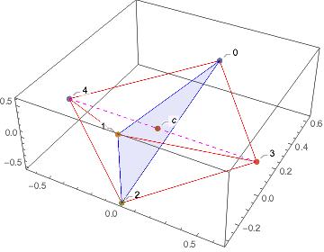
  $$U = 0.4062917146317[56,92]$$

  $$J = 0.2589744676461[55,92]$$

  $$x_{3} = 0.64538119213252[0,5]$$

  Figure 1: Diamond with triangular base, $n=5$

• a pyramid with square base Figure 2 , the square $q_{0}q_{3}q_{2}q_{4}$ with $q_{1}$ in the summit on the symmetry line; all triangular faces are equilateral; $c$ indicates the center of mass and this lie over the plane of the square; diagonals of the square are marked as dashed blue lines. This is called a square pyramid in [Ks00, Sec. 5.2.1] and appears as Fig. 3b in [LS09]

  

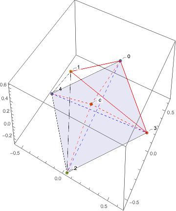
  $$U = 0.4066684332090[57,96]$$

  $$J = 0.2593347374996[26,70]$$

  $$x_{3} = 0.64031449289674[2,7]$$

  Figure 2: Pyramid with square base, $n=5$

• the regular tetrahedron (Figure 3) $q_{0}q_{1}q_{3}q_{4}$ with body $q_{2}$ at the origin, this is regular tetrahedron from [Ks00, Sec. 5.2.2] and appears as Fig. 4a in [LS09]

  

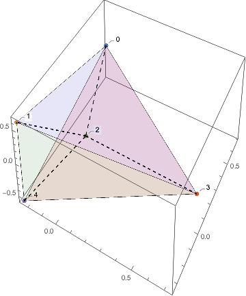
  $$U = 0.4224351404453[00,38]$$

  $$J = 0.2745617643612[04,48]$$

  $$x_{3} = 0.7266663096336[88,96]$$

  Figure 3: The regular tetrahedron, $n=5$

• triangle pyramid (”perturbed tetrahedron”) (Figure 4) with an equilateral triangle $q_{0}q_{1}q_{4}$ as the base and $q_{3}$ at the summit; $q_{2}$ is inside; c is at the origin. We identify it with the one discussed in [Ks00, Sec. 5.2.4] as degree $43$ solution , although no geometric description of the obtained central configuration has been given there. It appears as Fig. 4b in [LS09].

  

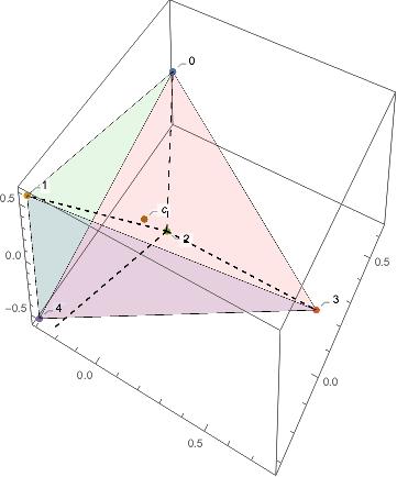
  $$U = 0.4222317695727[56,83]$$

  $$J = 0.2743635168460[37,68]$$

  $$x_{3} = 0.7779267783296[78,89]$$

  Figure 4: Perturbed tetrahedron, $n=5$

6.2 Six bodies

There are nine classes of non-coplanar central configurations:

1. diamond with a square base(Figure 5), two symmetrical pyramids with a common square base $q_{0}q_{4}q_{2}q_{5}$; $q_{1}$ is the summit of the upper pyramid, $q_{3}$ — the lower one. Points $q_{1}$, $q_{3}$ and $(0,0,0)$ (the center of mass) are collinear.

   

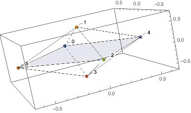
   $$U = 0.4253096183510[01,17]$$

   $$J = 0.2773689270621[74,91]$$

   $$x_{4} = 0.6521576637217[46,51]$$

   Figure 5: Diamond with a square base (item 1), $n=6$

2. diamond with regular triangular base (Figure 6), two tetrahedrons with a common equilateral triangle base $q_{0}q_{1}q_{3}$; $q_{2}=(0,0,0)$ lies at the triangle plane (i.e. bodies $q_{0}$, $q_{1}$, $q_{2}$ and $q_{3}$ are coplanar); $q_{4}$ is the summit of right pyramid, $q_{5}$ — the left one. Points $q_{2}$, $q_{4}$ and $q_{5}$ are collinear.

   

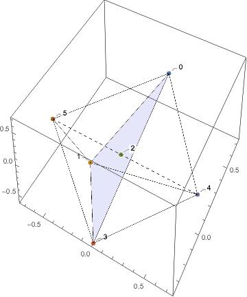
   $$U = 0.439099368866[330,431]$$

   $$J = 0.290967323607[179,293]$$

   $$x_{4} = 0.728578780778[797,824]$$

   Figure 6: Diamond with regular triangular base (item 2), $n=6$

3. two pyramids (one inside the other) (Figure 7) with a common square base $q_{0}q_{1}q_{3}q_{5}$; $q_{2}$ is the summit of inner pyramid, $q_{4}$ — the outer one. Points $q_{2}$, $q_{4}$ and $(0,0,0)$ (the center of mass) are collinear.

   

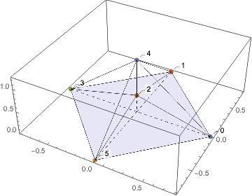
   $$U = 0.43903620010[0984,1039]$$

   $$J = 0.290904538096[071,137]$$

   $$x_{4} = 0.7893559716313[63,73]$$

   Figure 7: Two pyramids (item 3), $n=6$

4. two orthogonal isosceles triangles (Figure 8); altitudes of both triangles, points $q_{2}$, $q_{4}$ and the center of mass (point $(0,0,0)$) lie on the line marked red on the picture, which is an intersection line of the planes containing the triangles

   

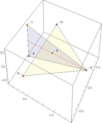
   $$U = 0.4388961044945[10,57]$$

   $$J = 0.290765308587[179,232]$$

   $$x_{4} = 0.7815214369079[53,63]$$

   Figure 8: Two orthogonal isosceles triangles (item 4) $n=6$

5. two pyramids (one inside the other) (Figure 9) with a common square base $q_{0}q_{1}q_{3}q_{5}$; $q_{2}$ is the summit of inner pyramid, $q_{4}$ — the outer one. Points $q_{2}$, $q_{4}$ and $(0,0,0)$ (the center of mass) are collinear.

   

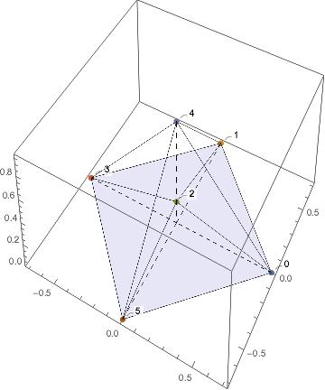
   $$U = 0.439337329879[509,619]$$

   $$J = 0.291203881424[758,879]$$

   $$x_{4} = 0.7268223700720[89,95]$$

   Figure 9: Two pyramids (item 5), $n=6$

6. pentagonal pyramid, (Figure 10) a polyhedron with a regular pentagon $q_{0}q_{4}q_{2}q_{5}q_{3}$ as a base; $q_{1}$ is the summit and is collinear with $(0,0,0)$ (the center of mass).

   

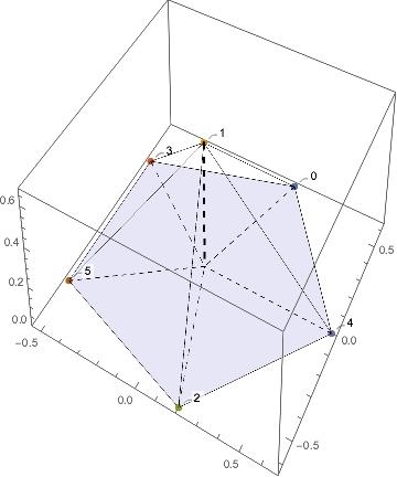
   $$U = 0.4327554322378[11,42]$$

   $$J = 0.2846844804120[32,68]$$

   $$x_{4} = 0.66271482439001[3,9]$$

   Figure 10: Pentagonal pyramid (item 6), $n=6$

7. a prism (Figure 11), a polyhedron with three rectangular and two triangular faces; $q_{0}q_{1}q_{4}$ and $q_{2}q_{3}q_{5}$ are symmetrical equilateral triangles, thus rectangles $q_{0}q_{1}q_{3}q_{5}$, $q_{0}q_{4}q_{2}q_{5}$ and $q_{1}q_{3}q_{2}q_{4}$ are also of the same size — lines with the same length have the same color (red or blue).

   

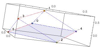
   $$U = 0.428444021033[087,122]$$

   $$J = 0.280440756454[764,805]$$

   $$x_{4} = 0.6545563543600[36,42]$$

   Figure 11: Prism (item 7), $n=6$

8. triangular polyhedron (Figure 12) with faces being isosceles triangles; $q_{0}q_{1}q_{4}$ and $q_{0}q_{1}q_{5}$ are symmetrical, $q_{0}q_{4}q_{5}$ has one side longer (the segment $(q_{4},q_{5})$ is longer than $(q_{0},q_{1})$); triangle $q_{0}q_{2}q_{3}$ is also an isosceles triangle; lines with the same length have the same color (red or blue).

   

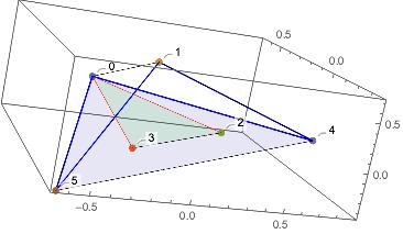
   $$U = 0.4583877507512[24,44]$$

   $$J = 0.3103483962997[44,68]$$

   $$x_{4} = 0.88496678932040[3,7]$$

   Figure 12: Triangular polyhedron (item 8), $n=6$

9. Diamond with triangular base, (Figure 13) two symmetrical polyhedrons with triangular base $q_{1}q_{4}q_{5}$ and with summits at $q_{0}$ and $q_{3}$; the center of mass ($(0,0,0)$) and the point $q_{2}$ lies on the plane of triangle $q_{1}q_{4}q_{5}$ and points $q_{0}$, $q_{3}$ are symmetrical with respect to that plane (i.e. triangle $q_{0}q_{2}q_{3}$ is isosceles); in the figure point $c$ is the center of mass $(0,0,0)$; lines with the same length have the same color (red, blue, magenta, green and orange).

   

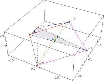
   $$U = 0.439320318180[620,757]$$

   $$J = 0.291186967912[789,943]$$

   $$x_{4} = 0.7520348731739[36,75]$$

   Figure 13: Diamond with isosceles triangular base (item 9) $n=6$

7 The number of non-equivalent CCs for mass parameters close to equal mass case

In this section we count the number of CCs (different equivalency classes of CCs) for mass parameters close to the equal mass case. This is possible because for the equal mass case all CCs turned out to be non-degenerate solutions of ${\cal RS}$ ​​. Then a simple continuation argument allows us to infer that the number of CCs does not change. A single CC for the equal mass case give rise (can be continued) to multiple CCs when the masses differ.

Example 1

Consider a square — one of the planar CCs for $n=4$. We distinguish bodies by (possibly different) masses and we show how many CCs for different masses we obtain. We use vertex labeling (coloring) for this purpose. To suggest different arrangement of masses we use $m_{1},\ldots,m_{4}$ colors. We identify those colorings which result from the application of planar isometry to a CC. In Figure 14 we present all three different arrangements of bodies for CC being a square under symmetry group $\mathcal{O}(2)$. Notice that there are 4! = 24 different colorings of a square by four colors $m_{1},\ldots,m_{4}$. However, some of them can be obtained from another by rotation or reflection. For example arrangement $m_{4}m_{1}m_{2}m_{3}$ can be obtained from $m_{1}m_{2}m_{3}m_{4}$ by rotating latter by $\pi/2$ angle.

Figure 14: All non-isomorphic (non-$\mathcal{O}(2)$ equivalent) colorings of a square with colors $m_{1},\ldots,m_{4}$.

If we use $\mathcal{SO}(2)$ as the symmetry group (we allow rotations and reject reflections) we obtain six colorings, i.e. six non-congruous CCs (see Figure 15).

Figure 15: All non-congruous (not $\mathcal{SO}(2)$-equivalent) colorings of a square with colors $m_{1},\ldots,m_{4}$.

Summarizing: if we use just rotations, then there is six non-equivalent CCs obtained from the square in the different masses case; if we additionally allow reflections, then we obtain only three non-equivalent CCs.

7.1 Definitions and Pólya’s theorem

We can count non-isomorphic colorings with the aid of Pólya’s enumeration theorem, see [B89] or [PTW83]) for the detailed treatment and proof. In this section we just recall the relevant definitions and state main theorems.

Let $X$ be a finite set with $|X|=n$ and $(G,\circ)$ be a subgroup of the group of permutations of $X$ with $\circ$ denoting the composition of permutations.

Coloring of $X$ is a function $\omega:X\to\mathcal{C}$, where $\mathcal{C}$ is a finite set of colors. We assume that the cardinality of $\mathcal{C}$ is $k$ and it is the only important feature of $\mathcal{C}$. Notice that any non-negative $k$ has a combinatorial sense, but in our counting problem we have to take $k=n$.

Definition 4

We say that two colorings $\omega_{1}$, $\omega_{2}$ are isomorphic with respect to group $G$, if there is a $g\in G$ such that

$$\omega_{1}(g(x))=\omega_{2}(x),\quad\forall x\in X.$$

Definition 5

An index of a permutation $g\colon X\to X$ is a function of $n$ variables

$$\zeta_{g}\left(x_{1},\ldots,x_{n}\right)=x_{1}^{\alpha_{1}}\cdot x_{2}^{\alpha_{2}}\cdot\ldots\cdot x_{n}^{\alpha_{n}},$$

where $\alpha_{i}$ is a number of cycles of permutation $g$ containing exactly $i$ elements for $i=1,2,\ldots,n.$

Definition 6

An index of a group $G$ is defined as

$$\zeta_{G}(x_{1},\ldots,x_{n})=\frac{1}{|G|}\sum_{g\in G}\zeta_{g}(x_{1},\ldots,x_{n}).$$

Theorem 5

The number of non-isomorphic colorings of $X$ with respect to group $G$ with $k$ colors is

$$\zeta_{G}\left(k,k,\ldots,k\right).$$

Example 2

Let $X=\{1,2,3,4\}$ be a square as in Figure 14. Let $(G_{\mbox{\sc\tiny RR}},\circ)$ be a group of all rotations and reflections (on a plane) of that square. Permutations in $G_{\mbox{\sc\tiny RR}}$, their decomposition in two cycles and their indices are:
$\begin{array}[]{l|l|lcl|p{75mm}}g_{0}&(1)(2)(3)(4)&\zeta_{g_{0}}(x_{1},x_{2},x_{3},x_{4})&=&x_{1}^{4}&identity\\ g_{1}&(1234)&\zeta_{g_{1}}(x_{1},x_{2},x_{3},x_{4})&=&x_{4}&rotation by $\pi/2$ \quad(one 4-elements cycle)\\ g_{2}&(13)(24)&\zeta_{g_{2}}(x_{1},x_{2},x_{3},x_{4})&=&x_{2}^{2}&rotation by $\pi$ \quad(two 2-elements cycles)\\ g_{3}&(1432)&\zeta_{g_{3}}(x_{1},x_{2},x_{3},x_{4})&=&x_{4}&rotation by $3\pi/2$ \quad(one 4-elements cycle)\\ g_{4}&(1)(3)(24)&\zeta_{g_{4}}(x_{1},x_{2},x_{3},x_{4})&=&x_{1}^{2}x_{2}&reflection with respect to line (13) \quad(two 1-element cycles, one 2-element cycle)\\ g_{5}&(13)(2)(4)&\zeta_{g_{5}}(x_{1},x_{2},x_{3},x_{4})&=&x_{1}^{2}x_{2}&reflection with respect to line (24)\\ g_{6}&(12)(34)&\zeta_{g_{6}}(x_{1},x_{2},x_{3},x_{4})&=&x_{2}^{2}&reflection with respect to line perpendicular to the segment (12)\quad(two 2-elements cycles)\\ g_{7}&(14)(23)&\zeta_{g_{7}}(x_{1},x_{2},x_{3},x_{4})&=&x_{2}^{2}&reflection with respect to line perpendicular to the segment (14).\end{array}$
Thus $G_{\mbox{\sc\tiny RR}}=\{g_{0},\ldots,g_{7}\}$, $|G_{\mbox{\sc\tiny RR}}|=8$ and its index is

$$\zeta_{G_{\mbox{\sc\tiny RR}}}(x_{1},x_{2},x_{3},x_{4})=\frac{1}{8}\left(x_{1}^{4}+3x_{2}^{2}+2x_{4}+2x_{1}^{2}x_{2}\right).$$

Hence the number of different coloring with $4$ colors is

$$\zeta_{G_{\mbox{\sc\tiny RR}}}(4,4,4,4)=\frac{1}{8}\left(4^{4}+4^{2}+2\cdot 4\right)=2360.$$

In this number there are all colorings with one, two, three and four colors, and this is not what we are interested in. We want to know a number of different colorings with exactly four colors. For this we need full version of Pólya’s enumeration Theorem.

Theorem 6 (Pólya’s enumeration Theorem)

Let $D$ be a set of all non-isomorphic colorings of a set $X$ with respect to $G$ with $k$ colors. Then the generating function $\mathcal{U}_{D}$

$$\mathcal{U}_{D}\left(x_{1},x_{2},\ldots,x_{k}\right)=\zeta_{G}\left(\sigma_{1},\sigma_{2},\ldots,\sigma_{n}\right),$$

where

$$\sigma_{i}=x_{1}^{i}+x_{2}^{i}+\ldots+x_{k}^{i},$$

has its coefficient at $x_{1}^{i_{1}}\ldots x_{k}^{i_{k}}$ equal to the number of non-isomorphic colorings using each of the colors $m_{1},\ldots,m_{k}$ exactly $i_{1},\ldots,i_{k}$ times, respectively.

Example 3

Consider the case from Example 2. The generating function is

$$\mathcal{U}(x_{1},x_{2},x_{3},x_{4}) = \zeta_{G_{\mbox{\sc\tiny RR}}}(x_{1}+x_{2}+x_{3}+x_{4},x_{1}^{2}+x_{2}^{2}+x_{3}^{2}+x_{4}^{2},$$ (45)

$$\quad\quad\quad x_{1}^{3}+x_{2}^{3}+x_{3}^{3}+x_{4}^{3},x_{1}^{4}+x_{2}^{4}+x_{3}^{4}+x_{4}^{4})$$

$$= \frac{1}{8}\Big{\{}\ (x_{1}+x_{2}+x_{3}+x_{4})^{4}+$$

$$\quad\quad 3(x_{1}^{2}+x_{2}^{2}+x_{3}^{2}+x_{4}^{2})^{2}+$$

$$\quad\quad 2(x_{1}^{4}+x_{2}^{4}+x_{3}^{4}+2x_{4}^{4})+$$

$$\quad\quad 2(x_{1}+x_{2}+x_{3}+x_{4})^{2}(x_{1}^{2}+x_{2}^{2}+x_{3}^{2}+x_{4}^{2})\Big{\}}$$

$$= x_{1}^{4}+\ldots+\textbf{3}x_{1}x_{2}x_{3}x_{4}+\ldots x_{4}^{4}$$

From the expansion above (45), we see that the number of non-isomorphic colorings with four colors, each used once, in the case of square is 3.

7.2 Identifications of CCs made for the main result — summary

Let us remind the essence of counting of CCs mentioned in Section 1.2: any CC can be obtained from one of the normalized CCs, found by the program, by a suitable composition of translation, scaling, rotation, reflection and permutation of bodies. The reasons for such situation are as follows.

1. First, in Section 2, we normalized central configurations to obtain isolated solutions. This means that we remove possibility of translation (establishing a center of mass $c=0$) and possibility of scaling symmetry (setting $\lambda=1$). However, the obtained system (3) can have $\mathcal{O}(3)$ and $\mathcal{SO}(3)$ symmetry, which excludes the use of Krawczyk’s method. This method requires non-degenerate solutions .

2. In Section 3.2, we introduce ${\cal RS}$ and after these treatments solutions found by our program have no longer neither $\mathcal{SO}(3)$ nor $\mathcal{O}(3)$ symmetry. But reflections by the planes and some permutations of bodies are still possible. In the case of equal masses two CCs that differ only by labeling of bodies are equivalent.

3. Thus we remove remaining symmetries and possible permutations of bodies by a procedure of unifications of solutions.

Thus, in the equal mass case we count configurations treating them as indistinct if they have the same geometrical form. In the context of the Póyla’s theorem this corresponds to taking the permutation group $G$ to be the whole of $\mathcal{S}_{n}$ or, equivalently, using just one color.

7.3 Number of CCs for different masses close to equal mass case

In the different masses case in the context of the Póyla’s theorem we use exactly $n$ colors. We consider two CCs equivalent, isomorphic or congruous, if one can be transformed into another by an element of $\mathcal{O}(d)$ or $\mathcal{SO}(d)$, respectively. Hence depending on whether we allow for reflections (i.e. $\mathcal{O}(d)$) or not ($\mathcal{SO}(d)$) we get different counts.

In the sequel by no-CC$(n)$ we denote the number of CCs obtained for the equal masses case, by $\mbox{iso}(n)$ is number of different non-isomorphic CCs and the number of non-congruous CCs is denoted by $\mbox{cong}(n)$. These numbers are obtained using Pólya’s enumeration Theorem for different groups. Tables 3 and 4 contain the number of different CCs inferred from our rigorous count of CCs. Data in Tables 3 and 4 suggest that the number of different CCs in the different mass case grow faster than $(n!)$.

Example 4

For $n=4$ in the planar case there are four different CCs (i.e. no-CC(4) = 4) and there are $12$ non-isomorphic configurations for collinear solution, $3$ for square, $4$ for equilateral triangle and $12$ for isosceles triangle (for detailed description of CCs see [MZ]), thus iso$(4)=12+3+12+4=31$. The count of non-congruous classes is as follows: $12$ non-congruous configurations for collinear solution, $6$ for square, $8$ for equilateral triangle and $24$ for isosceles triangle, thus $\mbox{cong}(4)=12+6+8+24=50$.

$n$	no-CC$(n)$	iso$(n)$	$\mbox{cong}(n)$	iso$(n)/n!$	$\mbox{cong}(n)/n!$
4	4	31	50	1.29167	2.0833
5	5	207	354	1.72500	2.9500
6	9	1992	3624	2.76667	5.0333
7	14	28080	53640	5.57143	10.6429

Table 3: The number of different CCs in 2D

$n$	no-CC$(n)$	iso$(n)$	$\mbox{cong}(n)$	iso$(n)/n!$	$\mbox{cong}(n)/n!$
4	5	32	52	1.33333	2.1667
5	9	257	454	2.14167	3.7833
6	18	3099	5838	4.30417	8.1083

Table 4: The number of different CCs in 3D

8 The question of stability for planar CCs

Now, consider a planar CC. It gives rise to a periodic orbit, where all bodies move on circles with the angular velocity $1$. This orbit becomes a fixed point in the rotating coordinate frame. The stability/instability of this fixed point and the circular periodic orbit is the same.

Let

$$J=\left[\begin{array}[]{cc}0&-1\\ 1&0\\ \end{array}\right].$$ (46)

Then $\exp(J\theta)=\left[\begin{array}[]{cc}\cos\theta&-\sin\theta\\ \sin\theta&\cos\theta\\ \end{array}\right]$ is a rotation by the angle $\theta$ in the plane $OXY$.

The link between coordinates in the inertial frame $x\in\mathbb{R}^{2}$ and the coordinates $q$ with respect to the rotating frame with the angular velocity equal to $1$ is

$$x=\exp(Jt)q.$$ (47)

The equations of motion in the rotating coordinate frame are [Si78]

$$\dot{q}_{i} = v_{i},$$ (48)

$$\dot{v}_{i} = -2Jv_{i}+q_{i}-\sum_{j\neq i}\frac{m_{j}(q_{i}-q_{j})}{r_{ij}^{3}}.$$ (49)

As was mentioned earlier each planar CC with $v_{i}=0$, $i=0,\dots,n-1$ is a fixed point of the system (48,49). We investigated numerically the linear stability of all CCs for $n=4,5,6,7$ and for some particular non-symmetric CCs for $n=8,9,10$ whose existence has been established in [MZ]. It turns out that all these CCs are linearly unstable. The computation of eigenvalues for the linearization of (48,49) has been done non-rigorously, but we are confident that this computation can be with some effort made rigorous.

References

• [AK12] A.Albouy, V.Kaloshin, Finiteness of central configurations of five bodies in the plane, Annals of mathematics 176 (2012), 535โ€“588
• [ADL] M. Alvarez, J. Delgado, J. LLibre, On the spatial central configurations of the 5-body problem and their bifurcations, DCDS S, 1 (2008), 505โ€“518
• [B89] N.L.Biggs, Discrete Mathematics, Oxford University Press 1989
• [FK] J. Ch. Faugรฉre and I. Kotsireas, Symmetry theorems for the Newtonian 4โ€“ and 5โ€“body problems with equal masses, Computer algebra in scientific computingโ€”CASCโ€™99, Springerโ€“Berlin (1999), 81โ€“92.
• [HJ11] M.Hampton and A.N.Jensen, Finiteness of spatial central configurations in the five-body problem, Cel. Mech. Dyn. Astron. 109 (2011), no. 4, 321โ€“332.
• [HM05] M.Hampton and R.Moeckel, Finiteness of relative equilibria of the four-body problem, Invent. math. 163 (2005), no. 2, 289โ€“312.
• [K69] R.Krawczyk, Newton-Algorithmen zur Besstimmung von Nullstellen mit Fehlerschranken, Computing, 4(1969) , 187โ€“201
• [Ks00] I.Kotsireas, Central Configurations in the Newtonian N-body Problem in Celestial Mechanics, Contemporary Mathematics 2000
• [KL02] I. Kotsireas and D. Lazard, Central configurations of the 5โ€“body problem with equal masses in threeโ€“dimensional space, J. Math. Sci., 108 (2002), 1119โ€“1138.
• [LS09] Tsung-Lin Lee, M.Santoprete, Central configurations of the five-body problem with equal masses, Celest Mech Dyn Astr (2009) 104:369โ€“381
• [MZ] M. Moczurad, P. Zgliczyล„ski, Central configurations in planar $n$-body problem for $n=5,6,7$ with equal masses, Celestial Mechanics and Dynamical Astronomy (2019) 131:46
• [Moe01] R.Moeckel, Generic finiteness for Dziobek configurations, Trans. Am. Math. Soc. 353, 4673โ€“4686 (2001)
• [Moe89] R.Moeckel, Some Relative Equilibria of N Equal Masses $N=4,5,6,7$, http://www-users.math.umn.edu/ย rmoeckel/research/CC.pdf
• [Moe] R.Moeckel, Central configurations, Scholarpedia, 9(4):10667,
http://www.scholarpedia.org/article/Central_configurations
• [Moe14] R.Moeckel, Lectures On Central Configurations, 2014, http://www-users.math.umn.edu/~rmoeckel/notes/CentralConfigurations.pdf
• [Mo66] R.E.Moore, Interval Analysis. Prentice Hall, Englewood Cliffs, N.J., 1966
• [N90] A.Neumeier, Interval methods for systems of equations. Cambridge University Press, 1990
• [PTW83] G.Pรณlya, R.E.Tarjan, D.R.Woods, Notes on Introductory Combinatorics, Birkhauser 1983
• [Sa80] D. Saari, On the role and properties of n-body central configurations. Cel. Mech. Dyn. Astron. 21 (1980) 9โ€“20
• [Si78] C.Simo, Relative equilibrium solutions in 4 body problem, Cel. Mech. Dyn. Astron. 18 (1978), 165โ€“184
• [Sm98] S.Smale, Mathematical problems for the next century, Mathematical Intelligencer 20 (1998), 7โ€“15
• [W41] A.Wintner, The Analytical Foundations of Celestial Mechanics, Princeton, N.J. Princeton University Press, 1941