Thermodynamical and dynamical equilibrium of a self-gravitating uncharged thin shell

Abstract

The dynamical stability of massive thin shells with a given equation of state (EOS) (both for the barotropic and non-barotropic case) is here compared with the results coming from thermodynamical stability. Our results show that the restrictions in the parameter space of equilibrium configurations of the shell following from thermodynamical stability are much more stringent that those obtained from dynamical stability. As a byproduct, we furnish evidence that the link between the maximum mass along a sequence of equilibrium configurations and the onset of dynamical stability is valid for EOS of the type $P=P(\sigma,R)$.

1 Introduction

Self-gravitating thin shells are solutions of a given gravitational theory describing two regions separated by an infinitesimally thin region where matter is confined. Such a system conjugates the notions of vacuum, typical of black holes, together with the presence of matter, which may be described via statistical mechanics and thermodynamics. Thin shells have been frequently employed to probe thermodynamical properties of black holes, see for instance York1986 ; Lemos2015 ; Lemos2015b ; Lemos2016 ; Lemos2017 and, since they can be taken to their own gravitational radius, they can be transformed into quasi-black holes Lemos2007 , and used to calculate black hole properties (see for instance Lemos_2011 ) . In view of these applications, it is important to determine whether relevant thin-shell configurations are stable, both thermodynamically and dynamically. The thermodynamic stability of a spherically symmetric thin shell in which the interior region is Minkowski’s spacetime and the exterior given by Schwarzschild’s geometry was studied in Martinez1996 , while the linear dynamical stability of such systems under radial perturbations was analyzed in Brady1991 for a linear EOS, and in Habib2017 for a general EOS. Since these two types of stability yield inequivalent restrictions on the parameter space Martinez1996 , we shall present here the results of imposing both types of stability on a neutral thin shell configuration, for different barotropic equations of state, and also for EOS of the type $P=P(\sigma,R)$. The latter have been used in various settings such as wormholes (see for instance Rahaman2007 ; Varela2013 ; Garcia2011 ), stars in Eddington-inspired Born-Infeld gravity Kim2014 and gravastars MartinMoruno2011 , and in cosmology Guo2005 ; Debnath2007 , among others. For a given EOS, we shall determine the region of the parameter space of equilibrium configurations of the shell compatible with both types of stability, and with the dominant energy condition (DEC). As a byproduct, we shall obtain evidence supporting the extension of the results linking the maximum mass with the onset of instability LeMaitre2019 to EOS of the type $P=P(\sigma,R)$.

The paper is organized as follows. In Section 2 we shall present a brief review of the relevant equations for the thin shell in equilibrium (mostly following Lemos2015 ). The equations obeyed by the perturbed shell for an EOS of the type $P=P(\sigma,R)$ will be introduced in Section 3. In Section 4 we shall present the analysis of the dynamical stability of the shells for different barotropic EOS, along with the corresponding $m(R)$ diagrams. Section 5 is devoted to a non-barotropic EOS. The restrictions following from thermodynamical stability are exhibited in Section 6. In Section 7 we determine the set of equilibrium states of the shell that are both dynamically and thermodynamically stable. Our closing remarks are presented in Section 8.

2 Junction conditions and properties of the thin-shell

Let us consider a two-dimensional timelike massive shell $\Sigma$ with radius $R$. The shell divides the spacetime in two parts: i) an inner region $r<R$, with flat geometry, and ii) an outer region $r>R$, in which the geometry is described by the Schwarzschild line element. In this way, we can express the metric in both regions as follows:

$$ds_{I}^{2}=-f_{I}{dt_{I}}^{2}+g_{I}dr^{2}+r^{2}d\Omega^{2}.$$ (1)

Here $I=o,i$ refers either to the outer or inner region, and the functions $f_{I}$ and $g_{I}$ are given by

$$f_{i}=g_{i}=1,\quad f_{o}={1-\frac{2m}{r}},\quad g_{o}=\left(1-\frac{2m}{r}\right)^{-1},$$ (2)

where $m$ is the ADM mass, $d\Omega^{2}\equiv d\theta^{2}+\sin{\theta}^{2}d\phi^{2}$.
The metric $h_{ab}$, defined on $\Sigma$, i.e. for $r=R$, is that of a 2-sphere, and can be written as

$$ds_{\Sigma}^{2}=h_{ab}dy^{a}dy^{b}=-d\tau^{2}+R^{2}(\tau)d\Omega^{2},$$ (3)

where $y^{a}=(\tau,\theta,\phi)$ and $R$ is a function of $\tau$, the proper time for an observer located on the shell, in the dynamical case. The application of the thin-shell formalism developed in Israel1966 to join the two spacetimes specified in Eqs. (1) and (2) requires the induced metric $h_{ab}$ to be continuous on the shell, and the discontinuity in the extrinsic curvature to be proportional to the stress-energy tensor on the shell, denoted by ${\cal S^{\mu}_{\>\nu}}$. The latter is given by the surface energy density $\sigma$ and the tangential pressure $p$ which, for a static shell, are as follows (see for instance Martinez1996 ):

$${{\cal S}^{\tau}}_{\tau} \equiv\sigma_{0}=\dfrac{1-\sqrt{1-\frac{2m_{0}}{R_{0}}}}{4\pi R_{0}},$$ (4)

$${{\cal S}^{\theta}}_{\theta}={{\cal S}^{\phi}}_{\phi} \equiv P_{0}=\frac{\sqrt{1-\frac{2m_{0}}{R_{0}}}-1}{8\pi R_{0}}+\frac{m_{0}}{8\pi R_{0}^{2}\sqrt{1-\frac{2m_{0}}{R_{0}}}},$$ (5)

where the subindex 0 means that the quantities are evaluated at the equilibrium configuration.
The proper mass of the shell, denoted by $M$, is given by $M=4\pi R_{0}^{2}\sigma_{0}$. The junction conditions also imply that the ADM mass is given by

$$m_{0}=M-\frac{M^{2}}{2R_{0}}.$$ (6)

Hence we can write

$$P_{0}(M,R_{0}) =\frac{M^{2}}{16\pi R_{0}^{2}(R_{0}-M)},$$ (7)

$$\sigma_{0}(M,R_{0}) =\frac{M}{4\pi R_{0}^{2}}.$$ (8)

We shall assume that $\sigma_{0}$ and $P_{0}$ are non-negative (hence $M>0$) and $R_{0}\geq 2m_{0}$ .
Notice that by inverting Eqs. (7) and (8) we obtain $R_{0}(P_{0},\sigma_{0})$ and $M(P_{0},\sigma_{0})$ respectively given by

$$R_{0}(P_{0},\sigma_{0}) =\frac{P_{0}}{\pi\sigma_{0}(\sigma_{0}+4P_{0})},$$ (9)

$$M(P_{0},\sigma_{0}) =\frac{4P_{0}^{2}}{\pi\sigma_{0}(\sigma_{0}+4P_{0})^{2}}.$$ (10)

Using Eqs. (6) and (10) it follows that

$$m_{0}(M,R_{0}) =4\pi\sigma_{0}R_{0}^{2}(1-2\pi\sigma_{0}R_{0}).$$ (11)

The final equations for the mechanical equilibrium of the shell are then

$$R_{0}(P_{0},\sigma_{0}) =\frac{P_{0}}{\pi\sigma_{0}(\sigma_{0}+4P_{0})},$$ (12)

$$m_{0}(P_{0},\sigma_{0}) =4\pi\sigma_{0}R_{0}^{2}(1-2\pi\sigma_{0}R_{0}).$$ (13)

These equations will be used in the analysis of the linear stability and to build the $m_{0}=m_{0}(R_{0})$ diagrams for a given EOS, as we shall see in Sect.4.
Before moving to the dynamical stability of the shell, let us introduce the redshift of the shell, defined as

$$k=\sqrt{1-\frac{2m_{0}}{R_{0}}}.$$ (14)

It follows that $M=R_{0}(1-k)$.

3 Dynamical stability

We shall outline here the steps that lead to the condition for the linear dynamical stability of the shells introduced in the previous section. While Eqs. (7) and (8) describe the equilibrium state of the shell, the corresponding expressions for a dynamical shell are (see for instance Habib2017 ; Garcia2011 ).

$$\sigma= \frac{1}{4\pi}\frac{\sqrt{f_{o}(R)+\dot{R}^{2}}-\sqrt{f_{i}(R)+\dot{R}^{2}}}{R},$$ (15)

$$P= \frac{1}{8\pi}\left[\frac{2\ddot{R}+f_{o}^{\prime}(R)}{2\sqrt{f_{o}(R)+\dot{R}^{2}}}-\frac{2\ddot{R}+f_{i}^{\prime}(R)}{2\sqrt{f_{o}(R)+\dot{R}^{2}}}\right.$$

$$+\left.\frac{\sqrt{f_{o}(R)+\dot{R}^{2}}-\sqrt{f_{i}(R)+\dot{R}^{2}}}{R}\right],$$ (16)

where $f_{i}(R)$ and $f_{o}(R)$ are defined in Eq. (2), and the overdot denotes the derivative with respect to $\tau$. These quantities obey the equation that follows from the conservation of ${\cal S}^{\mu}_{\;\nu}$, namely

$$\frac{d\sigma}{dR}+\frac{2}{R}(P+\sigma)=0.$$ (17)

A radial perturbation of an equilibrium configuration with $R=R_{0}$ causes $R$, $\sigma$ and $P$ to become functions of $\tau$. Assuming an EOS of the type $P=P(\sigma,R)$, it follows from Eqs. (15) and (17) that the evolution of the shell is governed by the equation Habib2017

$$\dot{R}+V(R,\sigma(R))=0,$$ (18)

where

$$V(R)= \frac{1}{2}\,({f_{i}}\left(R\right)+{f_{o}}\left(R\right))-{\frac{1}{64}}\,{\frac{\left({f_{i}}\left(R\right)-{f_{o}}\left(R\right)\right)^{2}}{{\pi}^{2}{R}^{2}\sigma\left(R\right)^{2}}}$$

$$-4\,{\pi}^{2}{R}^{2}\sigma\left(R\right)^{2}.$$ (19)

The linear stability of the shell can be studied by expanding the potential $V(R)$ around the equilibrium state up to second order in $x=R-R_{0}$, hence obtaining

$$\frac{d^{2}x}{d\tau^{2}}+\omega_{0}^{2}x=0.$$

Stability implies that

$$\omega_{0}^{2}\equiv\left.\frac{d^{2}V}{dR^{2}}\right|_{R_{0}}>0.$$ (20)

The calculation of $\omega_{0}^{2}$ involves $\frac{d\sigma}{dR}$ (which is given by Eq. (17)), and $\frac{d^{2}\sigma}{dR^{2}}$, which is obtained by taking the derivative of Eq. (17). For a general EOS of the type $P=P(R,\sigma)$, the $\omega_{0}^{2}$ is given by Habib2017 :

where $F_{0}\equiv\sqrt{f_{i0}}$, $H_{0}\equiv\sqrt{f_{o0}}$, and

$$\Omega_{10} \equiv\left.\frac{dP}{dR}\right|_{R_{0}},$$ (22)

$$\Omega_{20} \equiv\left.\frac{dP}{d\sigma}\right|_{R_{0}}.$$ (23)

The line dividing stability from instability is given by $\omega_{0}^{2}=0$ which, using Eq. (2), leads to the following expression for the critical values of $\Omega_{20}$:

$$\Omega_{20c} =\frac{A\;\Omega_{10c}+B}{D}$$ (24)

where

with $u\equiv\sqrt{R_{0}(R_{0}-2m_{0})}$. Eq. (24), valid for an arbitrary EOS of the form $P=P(\sigma,R)$, determines regions of stability in a certain space of parameters. In particular, in the barotropic case, $\Omega_{10}=0$, and $\Omega_{20c}=B/D$ defines the surface $\Omega_{20c}=\Omega_{20c}(m_{0},R_{0})$. Any equilibrium configuration with $(m_{0},R_{0})$ such that $\Omega_{20}$ is greater that $\Omega_{20c}$ will be stable . In the non-barotropic case, Eq. (24) defines a 3-d surface by $\Omega_{20c}=\Omega_{20c}(m_{0},R_{0},\Omega_{10c})$.
When a specific EOS is chosen, there are other constraints that must be taken into account. As we shall see in Section 4, using the equilibrium equations (4) and (5) for a given EOS, we can obtain the derivatives of the EOS as $\Omega_{10}=\Omega_{10}(m_{0},R_{0};\kappa)$, and $\Omega_{20}=\Omega_{20}(m_{0},R_{0};\kappa)$, where $\kappa$ denotes the parameters of the EOS. The EOS and the equilibrium equations also yield $m=m(R_{0};\kappa)$. Combining the latter with the equation (23) for $\Omega_{20}$ we obtain $\Omega_{20}=\Omega_{20}(R^{\prime}_{0})$, where $R_{0}^{\prime}$ is the radius of the equilibrium configuration normalized using the dimension-full parameter of the EOS. Using $m=m(R_{0};\kappa)$ and the equation for $\Omega_{10}$ in the equation (24) for $\Omega_{20c}$, we obtain $\Omega_{20c}=\Omega_{20c}(R^{\prime}_{0})$, The dynamically stable configurations for the given EOS will be those with $\Omega_{20}(R^{\prime}_{0})>\Omega_{20c}(R^{\prime}_{0})$. We shall consider in the next section the dynamical stability of the shell presented in Section 2 for several relevant examples of EOS.

4 Dynamical stability for different EOS and the $m_{0}=m_{0}(R_{0})$ curve.

Let us apply next the discussion of the previous section to several EOS of interest, to determine the regions of dynamical stability in the $m_{0}\times R_{0}$ plane, as well as the actual equilibrium states given by the $m_{0}=m_{0}(R_{0})$ curve. It is important to note that the results from the dynamical stability analysis we shall present are in agreement with the criterion of the maximum of the $m_{0}=m_{0}(R_{0})$ diagram, a fact that was proved in LeMaitre2019 for the case of a barotropic EOS. Our results suggest that the criterion is also valid for EOS of the form $P=P(\sigma,R)$. All the $m_{0}=m_{0}(R_{0})$ curves stop at the point where the DEC $P\leq\sigma$ ceases to be satisfied.

4.1 Quadratic and barotropic EOS

We shall start with the example of a barotropic EOS, given by

$$P=\beta\sigma^{2},$$ (25)

where $[\beta]=L$. Such an equation models the non-relati-vistic limit of a two-dimensional ideal Fermi gas at $T=0$, discussed in Subsection 4.2. The constant $\beta$ can be used to render dimensionless all the variables in the problem as follows: $\sigma^{\prime}=\beta\sigma$, $P^{\prime}=\beta P$, $R^{\prime}=R/\beta$, and $m^{\prime}=m/\beta$. In these variables, Eq. (25) reads $P^{\prime}=\sigma^{\prime 2}$. Substituting $P^{\prime}$ into Eq. (12) we obtain $\sigma_{0}=\sigma_{0}(R_{0})$ which, in dimensionless form, is given by

$$\sigma^{\prime}_{0}(R^{\prime}_{0})=\frac{1}{4}\left(\frac{1}{\pi R^{\prime}_{0}}-1\right).$$ (26)

Using $\sigma^{\prime}_{0}(R^{\prime}_{0})$ in Eq. (13) we obtain the corresponding $m_{0}^{\prime}(R_{0}^{\prime})$ relation:

$$m^{\prime}_{0}(R^{\prime}_{0})=\frac{1}{2}R^{\prime}_{0}\left(1-\pi^{2}R_{0}^{{}^{\prime}2}\right).$$ (27)

In the domain $R^{\prime}_{0}\geq 0$, the function $m_{0}^{\prime}(R_{0}^{\prime})$ has a maximum for $R^{\prime}_{0max}=1/\left(\pi\sqrt{3}\right)$, resulting in $m^{\prime}_{0max}=1/\left(3\pi\sqrt{3}\right)$. The $m^{\prime}_{0}=m^{\prime}_{0}(R^{\prime}_{0})$ curve for this case is shown in Fig. 1.

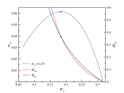
Figure 1: The figure shows the $m^{\prime}_{0}(R^{\prime}_{0})$ diagram for the EOS $P=\beta\sigma^{2}$, as well as the critical values of $\Omega_{2}$ that follow from dynamical stability (see Eq. (24)), and those that follow from the EOS, in red and blue, respectively.

In the low energy density limit $(\sigma^{\prime}\rightarrow 0)$, we can see that $m^{\prime}\rightarrow 0$ and $R^{\prime}\rightarrow 1/\pi$ (thus indicating that this EOS allows shells with very low mass). In the high energy density limit $(\sigma^{\prime}\rightarrow\infty)$, we have $m^{\prime}\rightarrow 0$ and $R^{\prime}\rightarrow 0$, however this region of the curve is not depicted because it violates the DEC. Notice also that $m_{0}(R^{\prime}_{0})$ given by (27) satisfies $2m^{\prime}_{0}<R^{\prime}_{0}$, which is a constraint from the theory of thin shells Lemos2015 .
Next we indicate how to obtain the curves for $\Omega_{20c}$ and $\Omega_{20}$ of Section 3. Using Eq. (27) in Eq. (24) with $\Omega_{10c}=0$, the curve $\Omega_{20c}=\Omega_{20c}(R^{\prime}_{0})$ follows, plotted in red in Fig. 1. For $\Omega_{20}$ we use that $\Omega_{20}\equiv\left.\frac{dP}{d\sigma}\right|_{0}=2\sigma^{\prime}_{0}$, where $\sigma^{\prime}_{0}$ is given by Eq. (26). This yields $\Omega_{20}=\Omega_{20}(R^{\prime}_{0})$, plotted in blue in Fig. 1. The curve $\Omega_{20}(R^{\prime}_{0})$ intersects $\Omega_{20c}(R^{\prime}_{0})$ exactly at the value of $R^{\prime}_{0}$ corresponding to the maximum of the $m^{\prime}_{0}(R^{\prime}_{0})$ curve, and all the configurations on the curve to the right of this point ($\Omega_{20}>\Omega_{20c}$) are stable.

4.2 A relativistic EOS (EOS I)

As shown in the Appendix, the EOS for a system of non-interacting relativistic fermions in 2d at $T=0$ is given by

$$\sigma_{0} =\frac{\alpha}{3\pi}\left[\left(x^{2}+1\right)^{3/2}-1\right],$$ (28)

$$P_{0} =\frac{\alpha}{3\pi}\left[\frac{1}{2}(x^{2}-2)\sqrt{x^{2}+1}+1\right],$$ (29)

with $x=p_{F}/mc$, $\alpha=mc^{2}/\lambda^{2}$ and $\lambda=\hbar/mc$. Following the same steps as in Subsection 4.1, where the dimensionless variables are now $\sigma^{\prime}=\sigma/\alpha$, $P^{\prime}=P/\alpha$, $R^{\prime}=\alpha R$, and $m^{\prime}=\alpha m$, we obtain the plots shown in Fig. 2.

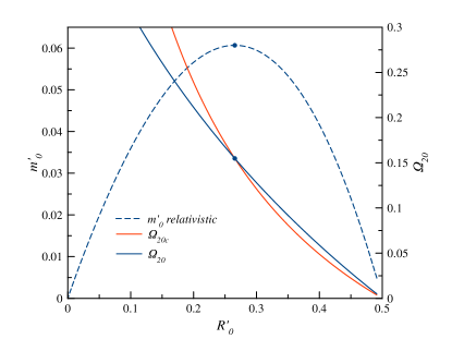
Figure 2: The figure shows the $m^{\prime}_{0}=m^{\prime}_{0}(R^{\prime}_{0})$ diagram for the relativistic EOS defined by Eqs. (28) and (29), as well as the critical values of $\Omega_{2}$ that follow from dynamical stability and those that follow from the EOS, in red and blue, respectively.

The values to the right of the maximum at $(R^{\prime}_{0max},m^{\prime}_{0max})=(0.26545,0.060666)$ are stable. In the low energy density limit $(\sigma^{\prime}\rightarrow 0)$, the plots show that $m^{\prime}\rightarrow 0$ and $R^{\prime}\rightarrow 0.5$ (indicating that this EOS also allows shells with very low mass), while in the high energy density limit $(\sigma^{\prime}\rightarrow\infty)$, $m^{\prime}\rightarrow 0$ and $R^{\prime}\rightarrow 0$. The DEC is satisfied along the whole curve as expected together with the constraint $2m_{0}^{\prime}<R_{0}^{\prime}$.

4.3 A more general barotropic EOS (EOS II)

Let us to study now the EOS II given by

$$P =\beta\sigma^{n},$$ (30)

where $[\beta]=L^{n-1}$. The case $n=2$ corresponds to the case studied in Subsection 4.1. Equations (12) and (13) now read

$$R_{0}(\sigma_{0}) =\frac{\beta\sigma_{0}^{n-2}}{\pi(1+4\beta\sigma_{0}^{n-1})},$$ (31)

$$m_{0}(\sigma_{0}) =4\pi\sigma R_{0}^{2}(1-2\pi\sigma_{0}R_{0}).$$ (32)

Defining the dimensionless quantities $\sigma^{\prime}$, $P^{\prime}$, $R^{\prime}$ and $m^{\prime}$ by

$$\sigma^{\prime} =\beta^{\frac{1}{n-1}}\sigma,$$ (33)

$$P^{\prime} =\beta^{\frac{1}{n-1}}P,$$ (34)

$$R^{\prime} =\beta^{\frac{1}{1-n}}R,$$ (35)

$$m^{\prime} =\beta^{\frac{1}{1-n}}m,$$ (36)

equations (30), (31) and (32) read

$$P_{0}^{\prime} =\sigma_{0}^{\prime n},$$ (37)

$$R_{0}^{\prime} =\frac{\sigma_{0}^{\prime n-2}}{\pi(1+4\sigma_{0}^{\prime n-1})},$$ (38)

$$m_{0}^{\prime} =4\pi\sigma_{0}^{\prime}R_{0}^{\prime 2}(1-2\pi\sigma_{0}^{\prime}R_{0}^{\prime}).$$ (39)

Equations (38) and (39) can be solved numerically to build the $m^{\prime}_{0}=m^{\prime}_{0}(R^{\prime}_{0})$ curves, an example of which is shown in Figure 3 (for $n=2.5$). The curves corresponding to $\Omega_{20c}$ and $\Omega_{20}$ are also shown. The stability interval goes from the maximum of the $m^{\prime}_{0}=m^{\prime}_{0}(R^{\prime}_{0})$ curve (which again coincides with the crossing of the $\Omega_{20}$ curves), all the way down to small values of $m^{\prime}_{0}$ and $R^{\prime}_{0}$.

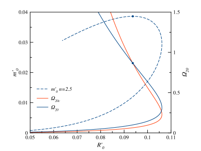
Figure 3: The figure shows the $m^{\prime}_{0}=m^{\prime}_{0}(R^{\prime}_{0})$ diagram for the EOS $P=\beta\sigma^{2.5}$, as well as the curves for $\Omega_{20c}$ and $\Omega_{20}$.

The upper panel of Fig. 4 shows the $m^{\prime}_{0}=m^{\prime}_{0}(R^{\prime}_{0})$ curves for $n=2.5,3.0,3.5,4.0,4.5$ (dashed line), the associated $k=k(R_{0})$ curves (Eq. (14)) for each case (full line), and the smallest value of $k$ ($k_{min}=1/5$) which satisfies the DEC (these curves will be useful below). The $\Omega_{20c}$ and $\Omega_{20}$ curves are displayed in the lower panel. In all cases, the maximum of the $m_{0}^{\prime}=m_{0}^{\prime}(R_{0}^{\prime})$ curve coincides with the crossing of the $\Omega_{2}$ curves. Also, all cases approach $m^{\prime}=R^{\prime}=0$ for $\sigma^{\prime}\rightarrow\infty$ (high-energy limit, not shown due to the DEC violation) and $\sigma^{\prime}\rightarrow 0$ (low-energy limit), and verify the condition $2m_{0}^{\prime}<R_{0}^{\prime}$. Notice also that in the dimensionless quantities we are using, all the $m_{0}^{\prime}=m_{0}^{\prime}(R_{0}^{\prime})$ curves end at the same point, where the DEC is marginally satisfied (i.e. $P_{0}^{\prime}=\sigma_{0}^{\prime}$).

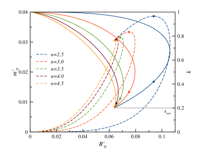
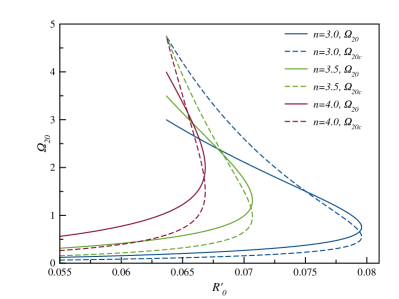
Figure 4: Upper panel: $m_{0}^{\prime}=m_{0}^{\prime}(R_{0}^{\prime})$ (dashed line) and $k=k(R_{0}^{\prime})$ curves (full line) for EOS II and several values of $n$. $k_{min}=1/5$ is the smallest value of $k$ which satisfies the DEC. Lower panel: plots of $\Omega_{20}$ and $\Omega_{20c}$ in terms of $R^{\prime}_{0}$ for different values of $n$ in EOS II.

5 A non-barotropic EOS (EOS III)

In this section we shall explore the dynamically stable equilibrium configurations that follow from the non-barotropic EOS given by Varela2013

$$P(\sigma,R) =\frac{A}{R^{n}}\sigma,$$ (40)

where $[A]=L^{n}$. Defining for convenience the dimensionless energy density, pressure, radius and mass as

$$\sigma^{\prime} =\sigma A^{1/n},$$ (41)

$$P_{0}^{\prime} =PA^{1/n},$$ (42)

$$R^{\prime} =\frac{R}{A^{1/n}},$$ (43)

$$m^{\prime} =\frac{m}{A^{1/n}},$$ (44)

and using the EOS in the equations for the mechanical equilibrium of the shell, given in Eqs. (12) and (13), the following $m_{0}^{\prime}(R_{0}^{\prime})$ relation is obtained:

$$m_{0}^{\prime}(R_{0}^{\prime}) =\frac{4R_{0}^{\prime}(R_{0}^{\prime n}+2)}{(R_{0}^{\prime n}+4)^{2}}.$$ (45)

The extremum is given at

$$R_{0m}^{\prime} =\left(\frac{3+\sqrt{8n+1}}{n-1}\right)^{1/n}\;\;\;,\;{\rm for}\;n>1.$$ (46)

The maximum in the $m_{0}^{\prime}=m_{0}^{\prime}(R_{0}^{\prime})$ diagram, is given by

$$m_{0max}^{\prime}=m_{0}^{\prime}(R_{0m}^{\prime})= 4(n-1)\left(\frac{3+\sqrt{8n+1}}{n-1}\right)^{1/n}$$

$$\left(\frac{\sqrt{8n+1}+2n+1}{\sqrt{8n+1}+4n-1}\right),\;\;n>1.$$ (47)

The $m^{\prime}_{0}=m^{\prime}_{0}(R^{\prime}_{0})$ curve for $n=3$ is shown in Fig. 5.

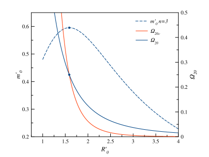
Figure 5: $m^{\prime}_{0}=m^{\prime}_{0}(R^{\prime}_{0})$ diagram, as well as $\Omega_{20}$ and $\Omega_{20c}$ curves for EOS III with $n=3$.

The stable equilibrium configurations are those located to the right of the maximum, in correlation with the crossing of the $\Omega_{2}$ curves. Notice that there are configurations with very small $m^{\prime}_{0}$ and very large $R^{\prime}_{0}$. The $m^{\prime}_{0}=m^{\prime}_{0}(R^{\prime}_{0})$ curves for several values of $n$ are shown in the upper panel of Fig. 6 (dashed line) together with the corresponding $k(R^{\prime}_{0})$ curves (full line) while the associated $\Omega_{2}$ curves are displayed in the lower panel. In all cases, the maximum of the $m_{0}^{\prime}=m_{0}^{\prime}(R_{0}^{\prime})$ curve coincides with the crossing of the $\Omega_{2}$ curves.

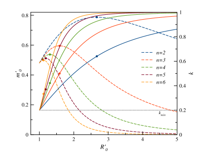
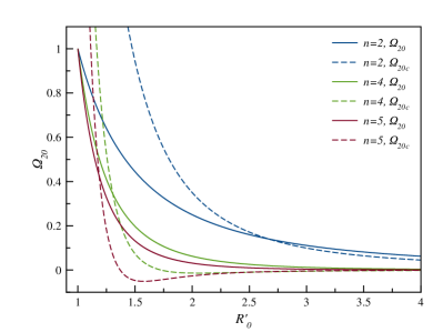
Figure 6: Upper panel: The figure shows the $m_{0}=m_{0}(R_{0})$ (dashed line) and $k=k(R_{0})$ curves (full line) for EOS III and several values of $n$. $k_{min}=1/5$ is the smallest value of $k$ which satisfies the DEC. Lower panel: $\Omega_{20}$ and $\Omega_{20c}$ curves for different values of $n$ for the non-barotropic EOS III.

6 Thermodynamical stability

We shall compare next the results presented in the previous sections (via dynamical stability) with those originating from thermodynamical stability. This type of stability was studied for the neutral shell in Martinez1996 . Two equations of state were used there, a phenomenological one for the temperature, and the one that follows from the junction conditions (Eq. (7)), to obtain the entropy of a thin shell with constant number of particles. Starting from the first law:

$$dS=\beta dM+pdA,$$ (48)

where $\beta\equiv 1/T$ and $A\equiv 4\pi R^{2}$, Martinez showed that, as a consequence of Eq. (7) and the integrability condition for $S$, the function $\beta$ must have the form

$$\beta(M,R)=b(r_{+})k,$$ (49)

where $b$ is an arbitrary function of $r_{+}(M,R_{0})=2m(M,R_{0})$, and $k$ is given in Eq. (14). The explicit form of the function $b$ should be obtained from an explicit model of the matter that composes the shell. The following phenomenological form was chosen in Martinez1996 :

$$b(r_{+};\eta,a)=\frac{2\eta}{{\ell_{P}}^{1+a}}\>r_{+}^{a},$$ (50)

where $\eta$ and $a$ are dimensionless coefficients. Such a choice leads to

$$S(M,R_{0};\eta,a)=\frac{\eta}{1+a}\left(\frac{r_{+}}{{\ell}_{P}}\right)^{1+a}+S_{0},$$ (51)

for $a\neq-1$. This expression reduces to the Bekenstein-Hawking entropy for $a=1$ and $\eta=2\pi$. By demanding that a zero mass shell possess null entropy, it follows that $S_{0}=0$ and $a>-1$.
The regions of thermodynamical stability in the $(M,R)$ plane are determined by the conditions

$$\left(\frac{\partial^{2}S}{\partial M^{2}}\right)_{A}\leq 0,$$ (52)

$$\left(\frac{\partial^{2}S}{\partial A^{2}}\right)_{M}\leq 0,$$ (53)

$$\left(\frac{\partial^{2}S}{\partial M^{2}}\right)_{A}\left(\frac{\partial^{2}S}{\partial A^{2}}\right)_{M}-\left(\frac{\partial^{2}S}{\partial M\partial A}\right)^{2}\geq 0.$$ (54)

As shown in Martinez1996 , these conditions are more concisely expressed in terms of $k$. Together with the normalization of the entropy and the DEC, they imply that

$$-1 <a\leq\frac{12}{19}$$

for a stable shell. For $-1<a\leq 0$ the stability conditions do not constrain the value of $k$, hence the sole constraint for stability is that coming from the dominant energy condition, namely $R\geq\frac{25}{24}r_{+}$, or $k\geq 1/5$. The stability condition with the crossed derivatives leads to

$$(3a+1)k^{2}+2ak+(a-1)\leq 0,$$ (55)

which is automatically satisfied for $a\leq 0$, but restricts the values of $k$ for $0<a\leq 12/19$.

7 Dynamical and thermodynamical stability

Before presenting the results for all the EOS considered here with the anzat of Eq. (50), let us give an example. Figure 7 shows the $m^{\prime}_{0}=m^{\prime}_{0}(R^{\prime}_{0})$ diagram for the EOS II with $n=2$, and the values of $k$ obtained from its definition, using the equilibrium curve $m^{\prime}_{0}=m^{\prime}_{0}(R^{\prime}_{0})$.

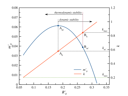
Figure 7: Dynamic and thermodynamic stability regions for EOS II with $n=2$ and $a=0.06$. The states with $k<k_{min}=1/5$ (which corresponds to $a>a_{max}=12/19$) violate the DEC. The allowed values of $k$ for thermodynamic stability satisfy $k_{min}<k<k_{max}$, where $k_{max}=0.843130$ follows from Eq. (55). The allowed values of $k$ for dynamical stability satisfy $k_{m^{\prime}}<k$, where $k_{m^{\prime}}=1/\sqrt{3}$ corresponds to the maximum of the curve $m^{\prime}_{0}=m^{\prime}_{0}(R^{\prime}_{0})$.

For the case at hand, such a curve is given by Eq. (27), which results in $k(R^{\prime}_{0})=\pi R^{\prime}_{0}$. The points that are dynamically stable are those on the curve to the right of $A_{m^{\prime}}$, which correspond to the interval $k>k_{m^{\prime}}=1/\sqrt{3}$. The thermodynamical stability region is $k_{min}<k<k_{max}$, where $k_{max}=0.843130$ is determined by Eq. (55) with $a=0.06$. Hence, the states that are both thermodynamically and dynamically stable are those between the points $A_{m^{\prime}}$ and $B_{m^{\prime}}$ in the $m^{\prime}_{0}=m^{\prime}_{0}(R^{\prime}_{0})$ curve. Figure 8 presents the region in the $(a,k)$ plane which correspond to configurations that are thermodynamically stable (which are those between the horizontal line $k_{min}$ and the curve $k_{max}=k_{max}(a)$), as well as that of dynamically stable configurations (which are those above the horizontal line $k_{m^{\prime}}$). The intersection of these regions yields the set of points $(a,k)$ associated to configurations that are both thermodynamically and dynamically stable.

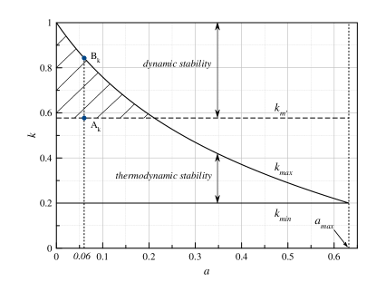
Figure 8: Dynamic and thermodynamic stability for EOS II with $n=2$ in the $(a,k)$ plane. The curve $k_{max}(a)$ follow from Eq. (55). The points $A_{k}$ and $B_{k}$ are those in Fig. 7.

Figure 9 presents the results in the $(a,k)$ plane for all the EOS we have examined.

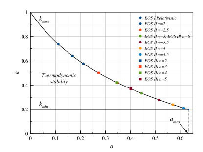
Figure 9: Dynamic and thermodynamic stability for all the EOS examined here. The states with $k<k_{min}=1/5$ (which corresponds to $a>a_{max}=12/19$) violate the DEC. The allowed values of $k$ for thermodynamic stability are those below the $k_{max}(a)$ curve, determined by Eq. 55, and above $k_{min}$. The allowed values of $k$ for dynamical stability are those above the value of $k$ on the curve for each EOS, which corresponds to the value of $k_{m^{\prime}}$ of the maximum of the curve $m^{\prime}_{0}=m^{\prime}_{0}(R^{\prime}_{0})$ for each EOS.

For a given value of $a$, the thermodynamically stable configurations are those with $k_{min}<k<k_{max}$. Also shown in the plot are the points at which the horizontal line associated to the value of $k$ corresponding to the maximum of the $m^{\prime}_{0}=m^{\prime}_{0}(R^{\prime}_{0})$ curve ($k_{m^{\prime}}$) intersects the $k_{max}=k_{max}(a)$ curve, obtained from Eq. (55). For a given EOS, the configurations that are both thermodynamically and dynamically stable are those above the horizontal line that crosses the corresponding point and below the $k_{max}=k_{max}(a)$ curve. The plot clearly shows that the requirement of thermodynamical stability greatly restricts the region of the parameter space allowed by the dynamical stability. It also follows from our results that the region associated to dynamical stability is larger for larger values of $n$, for both types of EOS considered here. This is to be expected since a larger $n$ is associated with more stiff matter.

8 Closing remarks

We have examined the dynamical and thermodynamical stability of neutral mass shells for different equations of state, described by $P=P(\sigma,R)$. To attain this goal, the condition for dynamical stability valid for an arbitrary EOS (obtained in previous works) given in terms of the derivatives $\Omega_{1}=\frac{dP}{dR}$ and $\Omega_{2}=\frac{dP}{d\sigma}$ was adapted to the case of a given EOS, yielding the curve $\Omega_{20c}=\Omega_{20c}(R_{0}^{\prime})$. The result was compared to the $\Omega_{2}=\Omega_{2}(R_{0}^{\prime})$ curve that follows from the given EOS and the equations for a shell in equilibrium, to determine the dynamically stable configurations. Using the criteria for thermodynamical stability and a specific form for the entropy of the shell, the set of thermodynamically stable configurations was also determined. The main result is that thermodynamical stability greatly constraints set of stable equilibrium configurations determined by dynamical stability, due to the upper constraint defined by Eq. (55). Our results also confirm that stable states are those to the right of the maximum of the $m^{\prime}_{0}=m^{\prime}_{0}(R^{\prime}_{0})$ curve. Such a link between the maximum mass along a sequence of equilibrium configurations of the shell and the onset of stability was obtained in LeMaitre2019 for the case of a barotropic EOS. Our findings suggest that it can be extended to EOS of the type $P=P(\sigma,R)$.
The generalization and consequences of our results to the interesting cases of self-gravitating shells in $d$ dimensions Andre2019 , and charged Lemos2015 and rotating Lemos2015c shells are left for future work.

Appendix: 2d fermion gas

We obtain here the EOS of a two-dimensional relativistic ideal Fermi gas of $N$ particles of mass $m$ at $T=0$ in a square of side $L$. In the thermodynamical limit we have $L\rightarrow\infty$, $N\rightarrow\infty$ and the particle number density $n=N/L^{2}$ constant.
For the summation over states $q$, we have in the continuous case

$$\sum_{q}\longrightarrow\frac{2L^{2}}{h^{2}}\int d^{2}p,$$

where $p$ is the two-dimensional linear momentum. Then, for the particle number density $n=N/L^{2}$ we have

$$N =\frac{2L^{2}}{h^{2}}\int_{0}^{p_{F}}d^{2}p=\frac{L^{2}}{2\pi\hbar^{2}}p_{F}^{2},$$

$$n =\frac{p_{F}^{2}}{2\pi\hbar^{2}}=\frac{x^{2}}{2\pi\lambda^{2}},$$ (56)

where $p_{F}$ is the Fermi momentum, $x=p_{F}/mc$, and $\lambda=\hbar/mc$ is the Compton wavelength.
Now we obtain the internal energy density $\sigma$. For the internal energy $U$ of the gas we have

$$U =\frac{2L^{2}2\pi}{h^{2}}\int_{0}^{p_{F}}\sqrt{p^{2}c^{2}+m^{2}c^{4}}\,p\,dp$$

$$\sigma =U/L^{2}=\frac{1}{\pi\hbar^{2}}\int_{0}^{p_{F}}\sqrt{p^{2}c^{2}+m^{2}c^{4}}\,p\,dp,$$

$$\sigma =\frac{mc^{2}}{3\pi\lambda^{2}}\left[\left(x^{2}+1\right)^{3/2}-1\right].$$ (57)

For the pressure we have

$$P =\frac{1}{2}\frac{1}{\pi\hbar^{2}}\int_{0}^{p_{F}}\frac{p^{2}c^{2}}{\sqrt{p^{2}c^{2}+m^{2}c^{4}}}\,p\,dp,$$

$$P =\frac{mc^{2}}{3\pi\lambda^{2}}\left[\frac{1}{2}(x^{2}-2)\sqrt{x^{2}+1}+1\right].$$ (58)

Finally, the EOS for a two-dimensional ideal relativistic Fermi gas at $T=0$ is given by

$$n =\frac{x^{2}}{2\pi\lambda^{2}},$$ (59)

$$\sigma =\frac{mc^{2}}{3\pi\lambda^{2}}\left[\left(x^{2}+1\right)^{3/2}-1\right],$$ (60)

$$P =\frac{mc^{2}}{3\pi\lambda^{2}}\left[\frac{1}{2}(x^{2}-2)\sqrt{x^{2}+1}+1\right].$$ (61)

References

- (1) J.W. York, Jr., Phys. Rev. D33, 2092 (1986). DOI 10.1103/PhysRevD.33.2092
- (2) J.P.S. Lemos, G.M. Quinta, O.B. Zaslavski, Phys. Rev. D91(10), 104027 (2015). DOI 10.1103/PhysRevD.91.104027
- (3) J.P.S. Lemos, G.M. Quinta, O.B. Zaslavskii, Phys. Lett. B750, 306 (2015). DOI 10.1016/j.physletb.2015.08.065
- (4) J.P.S. Lemos, G.M. Quinta, O.B. Zaslavskii, Phys. Rev. D93(8), 084008 (2016). DOI 10.1103/PhysRevD.93.084008
- (5) J.P.S. Lemos, M. Minamitsuji, O.B. Zaslavskii, Phys. Rev. D96(8), 084068 (2017). DOI 10.1103/PhysRevD.96.084068
- (6) J.P.S. Lemos, O.B. Zaslavskii, Phys. Rev. D76, 084030 (2007). DOI 10.1103/PhysRevD.76.084030
- (7) J.P. Lemos, O.B. Zaslavskii, Physics Letters B 695(1-4), 37–40 (2011). DOI 10.1016/j.physletb.2010.11.033. URL http://dx.doi.org/10.1016/j.physletb.2010.11.033
- (8) J. Kijowski, G. Magli, D. Malafarina, General Relativity and Gravitation 38(11), 1697 (2006). DOI 10.1007/s10714-006-0323-0. URL https://doi.org/10.1007/s10714-006-0323-0
- (9) E.A. Martinez, Phys. Rev. D53, 7062 (1996). DOI 10.1103/PhysRevD.53.7062
- (10) P.R. Brady, J. Louko, E. Poisson, Phys. Rev. D 44, 1891 (1991). DOI 10.1103/PhysRevD.44.1891. URL https://link.aps.org/doi/10.1103/PhysRevD.44.1891
- (11) S. Habib Mazharimousavi, M. Halilsoy, S.N. Hamad Amen, Int. J. Mod. Phys. D26(14), 1750158 (2017). DOI 10.1142/S0218271817501589
- (12) F. Rahaman, M. Kalam, S. Chakraborty, Acta Phys. Polon. B40, 25 (2009)
- (13) V. Varela, Phys. Rev. D92, 044002 (2015). DOI 10.1103/PhysRevD.92.044002
- (14) N.M. Garcia, F.S.N. Lobo, M. Visser, Phys. Rev. D86, 044026 (2012). DOI 10.1103/PhysRevD.86.044026
- (15) H.C. Kim, Phys. Rev. D 89, 064001 (2014). DOI 10.1103/PhysRevD.89.064001. URL https://link.aps.org/doi/10.1103/PhysRevD.89.064001
- (16) P. Martin Moruno, N. Montelongo Garcia, F.S. Lobo, M. Visser, JCAP 03, 034 (2012). DOI 10.1088/1475-7516/2012/03/034
- (17) Z.K. Guo, Y.Z. Zhang, Phys. Lett. B645, 326 (2007). DOI 10.1016/j.physletb.2006.12.063
- (18) U. Debnath, Astrophys. Space Sci. 312, 295 (2007). DOI 10.1007/s10509-007-9690-6
- (19) P. LeMaitre, E. Poisson, Am. J. Phys. 87(12), 961 (2019). DOI 10.1119/10.0000026
- (20) W. Israel, Il Nuovo Cimento B Series 10 44(1), 1 (1966). DOI 10.1007/bf02710419. URL https://doi.org/10.1007/bf02710419
- (21) R. André, J.P. Lemos, G.M. Quinta, Phys. Rev. D 99(12), 125013 (2019). DOI 10.1103/PhysRevD.99.125013
- (22) J.P.S. Lemos, F.J. Lopes, M. Minamitsuji, J.V. Rocha, Phys. Rev. D 92(6), 064012 (2015). DOI 10.1103/PhysRevD.92.064012