deepSIP: Linking Type Ia Supernova Spectra to Photometric Quantities with Deep Learning

Abstract

We present deepSIP (deep learning of Supernova Ia Parameters), a software package for measuring the phase and — for the first time using deep learning — the light-curve shape of a Type Ia supernova (SN Ia) from an optical spectrum. At its core, deepSIP consists of three convolutional neural networks trained on a substantial fraction of all publicly-available low-redshift SN Ia optical spectra, onto which we have carefully coupled photometrically-derived quantities. We describe the accumulation of our spectroscopic and photometric datasets, the cuts taken to ensure quality, and our standardised technique for fitting light curves. These considerations yield a compilation of 2754 spectra with photometrically characterised phases and light-curve shapes. Though such a sample is significant in the SN community, it is small by deep-learning standards where networks routinely have millions or even billions of free parameters. We therefore introduce a data-augmentation strategy that meaningfully increases the size of the subset we allocate for training while prioritising model robustness and telescope agnosticism. We demonstrate the effectiveness of our models by deploying them on a sample unseen during training and hyperparameter selection, finding that Model I identifies spectra that have a phase between $-10$ and 18 d and light-curve shape, parameterised by $\Delta m_{15}$, between 0.85 and 1.55 mag with an accuracy of 94.6%. For those spectra that do fall within the aforementioned region in phase–$\Delta m_{15}$ space, Model II predicts phases with a root-mean-square error (RMSE) of 1.00 d and Model III predicts $\Delta m_{15}$ values with an RMSE of 0.068 mag.

1 Introduction

The optical spectra of Type Ia supernovae (SNe Ia) are rich with information (for a review, see, e.g., Filippenko, 1997). In addition to probing ejecta dynamics and chemical composition, spectral features have been found to encode the phase of a SN Ia in its temporal evolution (e.g., Riess et al., 1997; Foley et al., 2005; Howell et al., 2005; Blondin & Tonry, 2007; Muthukrishna et al., 2019a), and to a somewhat less quantitatively formalised extent, its peak luminosity (Nugent et al., 1995; Arsenijevic et al., 2008; Bailey et al., 2009; Blondin et al., 2011; Silverman et al., 2012b; Zheng et al., 2018; Siebert et al., 2019). The ability to extract the former (henceforth, the “phase”) and the latter (or something that correlates with it via a width-luminosity relation, such as $\Delta m_{15}$ or $\Delta$; Phillips, 1993; Riess et al., 1996, respectively) from optical spectra is of particular significance because both are conventionally derived from photometry. As the requisite light curves must consist of numerous individual observations conducted over at least several weeks, the ability to measure the aforementioned quantities from perhaps just a single observation (i.e., a spectrum) is of great value when allocating limited observing resources to optimise for specific science goals.

The SuperNova IDentification code (SNID; Blondin & Tonry, 2007) has become the de facto tool for classifying the type and phase of a SN from spectra, though alternatives do exist (e.g., Superfit; Howell et al., 2005). To determine the phase of a SN Ia, such conventional approaches compare an input spectrum to a large database of spectra with known phases and then perform an aggregation of the phases from the best-matching templates. This approach has the advantage of being easy to understand (“SN X is most similar to SN Y at Z days relative to maximum brightness”), but it has the disadvantage of being inherently slow — prediction time scales linearly with the number of template spectra in the database.

Machine learning (ML; see Ivezić et al., 2014, for an overview of use cases in astronomy) provides an interesting and fundamentally different approach to these tasks. In particular, phase and light-curve-shape determination can both be treated within the “supervised learning” paradigm, where a robust mapping between inputs and outputs is derived from a training set of input-output pairs. Subject to passing user-defined efficacy criteria when applied to a distinct testing set, the derived map can then be deployed to characterise new, unseen data. This approach leads to predictions that are fast (i.e., based on features themselves instead of comparisons against a large database) and therefore scalable. Accordingly, supervised ML has become increasingly prevalent in astronomical research campaigns (e.g., Bloom et al., 2012; Masci et al., 2014; Goldstein et al., 2015; Wright et al., 2015; Miller et al., 2017; Kim & Brunner, 2017; Zhang & Bloom, 2020).

Indeed, ML has proven to be a viable approach to photometric SN classification (e.g., Richards et al., 2012; Möller et al., 2016; Lochner et al., 2016; Charnock & Moss, 2017; Narayan et al., 2018; Muthukrishna et al., 2019b), but only several studies thus far have applied such techniques to SN spectra. Sasdelli et al. (2016) use unsupervised ML techniques to explore the spectroscopic diversity of SNe Ia, and find that much of the spectral variability, including that of the peculiar SN 1991bg-like (Filippenko et al., 1992; Leibundgut et al., 1993) and SN 2002cx-like (now known as the distinct “SN Iax” class; Filippenko, 2003; Li et al., 2003; Foley et al., 2013) objects, can be parameterised by a carefully constructed five-dimensional space. As a much faster alternative to the aforementioned template-matching options (i.e., SNID, Superfit), Muthukrishna et al. (2019a) have used a deep convolutional neural network (CNN; see, e.g., LeCun et al., 2015) to develop DASH, a software package that classifies the type, phase, redshift, and host galaxy (but not light-curve shape) of a supernova from optical spectra.

Motivated by this and the well-documented ability of CNNs to extract representative low-dimensional features from input signals, we formulate our approach as a set of three models, each of which utilises a similar CNN architecture to (Model I) determine if an input spectrum belongs to a SN Ia within a specific domain in a space defined by phase and light-curve shape, (Model II) calculate the phase if it is within the domain, and (Model III) calculate a measure of the light-curve shape ($\Delta m_{15}$; Burns et al., 2011) if the same criterion is met. Although Model II shares a common objective and architectural elements with DASH (i.e., phase determination via a CNN architecture), we optimise specifically for SNe Ia that fall within certain thresholds, treat the problem as one of regression (not classification), and utilise dropout variational inference as a method by which to model uncertainties (Gal & Ghahramani, 2015; Leung & Bovy, 2019). Moreover, our development of a CNN to predict the light-curve shape of a SN Ia from its spectrum is novel.

We use the following sections to present the development of the aforementioned models. Section 2 details the accumulation of our dataset, including how we process and prepare spectra for ingestion by our models. We outline our model architecture and discuss training and hyperparameter selection procedures in Section 3, and we provide model-specific results in Section 4. Concluding remarks are then given in Section 5.

2 Data

2.1 Spectra

We source the spectra used herein from the three largest low-redshift SN Ia spectral datasets currently in existence: the Berkeley SuperNova Ia Program (BSNIP; Silverman et al., 2012a; Stahl et al., 2020, henceforth S12 and S20, respectively) sample with a total of 1935 spectra covering the period from 1989 through 2018 (see S12 for 1989–2008 and S20 for 2009–2018), the Harvard-Smithsonian Center for Astrophysics (CfA) sample with a total of 2603 spectra from observations spanning 1993–2008 (Blondin et al., 2012), and the Carnegie Supernova Program (CSP) sample with 630 spectra observed in the range 2004–2009 (Folatelli et al., 2013). From this initial compilation of 5168 spectra, we perform two modest “usability” cuts that reduce our sample to 4941 (these cuts, in addition to those that are introduced below, are outlined in Figure 1). First, we drop the small fraction without a redshift listed in their associated publication, thereby yielding 5110 spectra, and second, we remove a further 169 that lack full coverage of the Si ii $\uplambda 6355$ feature that is ubiquitous in near-maximum-light SN Ia spectra.

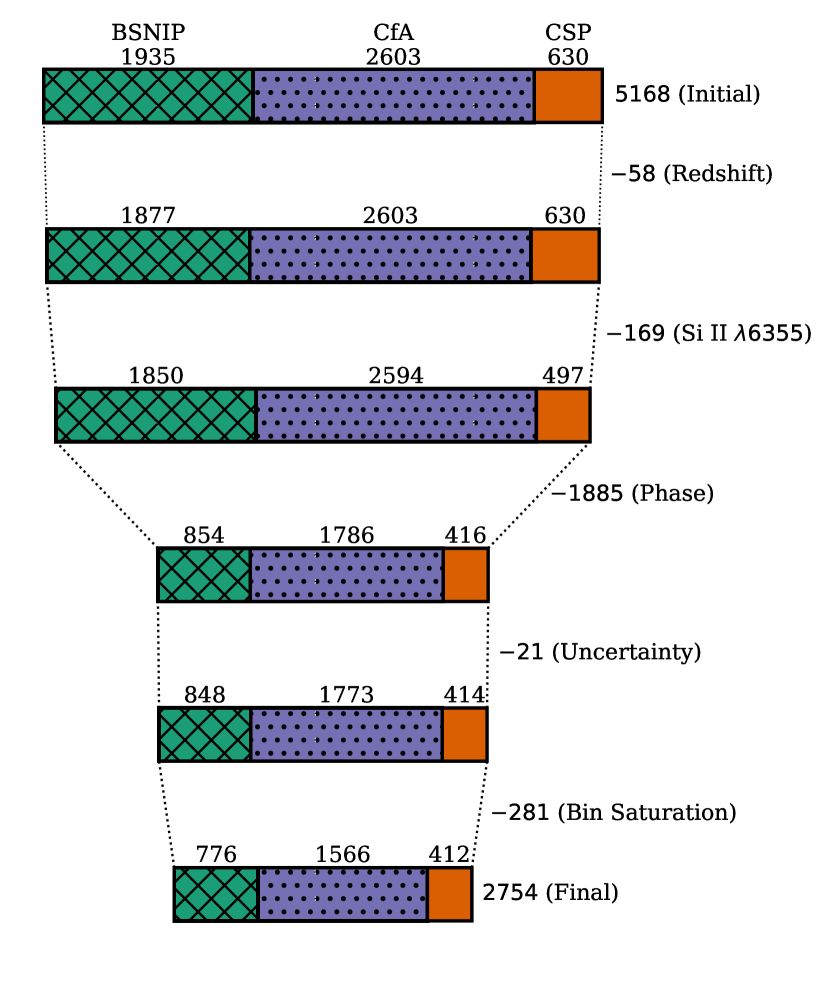
Figure 1: Full accounting of all cuts made in distilling our initial set of 5168 spectra down to the 2754 in our final compilation (1113 of which are within the “domain” defined in Section 2.3). We delineate the source of each spectrum in the top row. By a wide margin, the lack of suitable photometric observations is responsible for the most severe cut (indicated with “Phase”).

In addition to the high quality and sheer size of these datasets, the BSNIP and CfA sets were specifically selected for their complementarity — whereas the observing strategy employed by the BSNIP is generally to prioritise the total number of SNe observed instead of the number of spectra per SN, the CfA dataset covers fewer SNe but with higher cadence. This is clearly seen in the distribution of the number of spectra per SN in the top panel of Figure 2: the BSNIP sample spans many more SNe with several observations than does the CfA (or CSP) sample, but beyond $\sim 6$ spectra per object, the CfA sample wins out. Together, then, these datasets offer comprehensive coverage of the spectral diversity of SNe Ia at both the individual and population levels.

We show the distribution of blue (red) wavelength limits for the spectra in our compilation in the lower panel of Figure 2. The superior red-wavelength coverage of the Kast double spectrograph on the 3 m Shane telescope at Lick Observatory (responsible for $\sim 79\%$ of the BSNIP sample; Miller & Stone, 1993) to that of the FAST spectrograph on the 1.5 m Tillinghast telescope at Whipple Observatory (responsible for $\sim 94\%$ of the CfA sample; Fabricant et al., 1998) is evident. The Lick spectra as well as most from CSP have good relative spectrophotometry owing to the slit being placed at the parallactic angle (Filippenko, 1982), but the continuum shapes of the FAST spectra may be inaccurate in some cases since the slit could not be rotated to arbitrary parallactic angles. Because any heterogeneities in the inputs to our models should reflect only physically significant information, we formulate our data preprocessing and augmentation procedures (see Sections 2.3.2 & 2.3.3, respectively) to obscure as much source-specific information and contamination (e.g., wavelength limits, inaccurate continuum shapes) as possible.

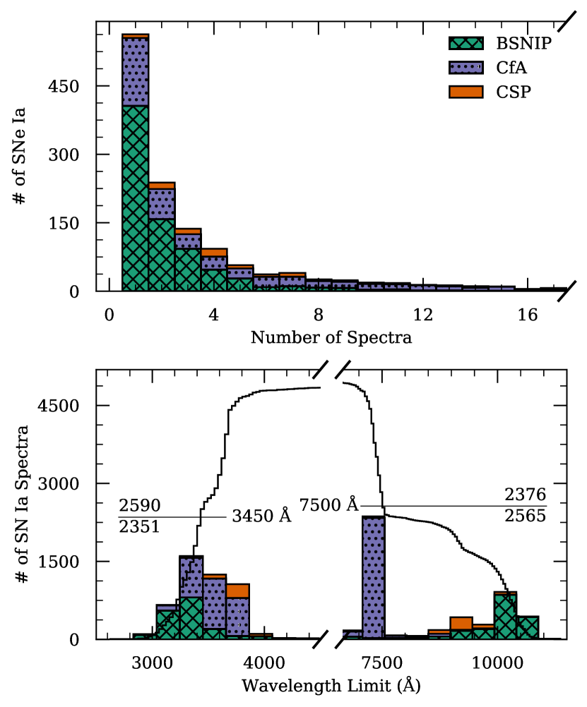
Figure 2: Stacked distributions of dataset parameters for our spectral compilation, distinguished by source. The top panel shows the number of spectroscopic observations per object (the tail extends to higher numbers of spectra, but is truncated for clarity) and the bottom panel displays the blue and red wavelength limits of the spectra. Overlaid on the bottom panel is the cumulative (inverse-cumulative) distribution of blue (red) wavelength limits, and the intersecting horizontal lines reflect the bounds defined in Section 2.3.2. The number of spectra above and below each intersecting line are also labeled.

2.2 Light curves

As the purpose of this study is to identify and therefore derive, through supervised learning, certain photometrically-derived properties encoded in SN Ia spectra, the aforementioned spectral compilation must be coupled to photometric observations (i.e., light curves), thereby allowing for the desired properties to be measured. To this end, we collect the requisite information from data releases by the same groups responsible for our compilation of spectra (Ganeshalingam et al., 2010; Stahl et al., 2019; Riess et al., 1999; Jha et al., 2006; Hicken et al., 2009; Krisciunas et al., 2017, henceforth G10 and S19 for the Berkeley sample, CfA1-3 for the CfA sample, and CSP3 for the CSP sample, respectively), as well as publish several new light curves (see Appendix A). We use the $E(B-V)$ model implemented within the SNooPy package (Burns et al., 2011, see Appendix B for additional details) to fit the aforementioned light curves (except for those from S19 and CSP3, who have published fits using the same procedure along with their photometry), allowing us to measure the time of maximum B-band brightness (and hence the phase) and the decline-rate parameter, $\Delta m_{15}$.

2.3 Final Compilation

All told, 3056 spectra are linked to light curves with successful SNooPy fits, but as shown in Figure 1, we remove 21 spectra having a phase uncertainty in excess of 1 day (d) and/or a $\Delta m_{15}$ uncertainty exceeding 0.1 mag, thus yielding 3035 spectra. We visualise this compilation within the photometric parameter space of interest (namely, $\Delta m_{15}$ and phase) in Figure 3. Unsurprisingly, the densest coverage — by a wide margin — occurs for $\Delta m_{15}\approx 1.1$ mag (reflecting that of a prototypical SN Ia), but particularly impressive is the coverage within the region defined by $-10\lesssim{\rm phase}\lesssim 18$ d and $0.85\lesssim\Delta m_{15}\lesssim 1.55$ mag (albeit a bit sparse for the more rapidly declining objects within this region).

Motivated by this coverage, we impose the aforementioned region as a “domain” on our models in the following way: Model I is tasked with classifying whether an input spectrum lies within its boundaries, while Model II and Model III determine the phase and $\Delta m_{15}$ (respectively) for spectra within this restricted domain. To mitigate the imbalance caused by the dominance of samples with $\Delta m_{15}\approx 1.1$ mag, we enforce a “saturation point” of 40 samples for each in-domain bin in Figure 3. According to this policy, overly dense bins are brought into compliance by removing spectra with the largest $\Delta m_{15}$ uncertainties until only 40 remain. A total of 281 spectra are removed by this action, leaving 2754 examples (1113 of which are in-domain and thus relevant to Models II & III) in what will henceforth be referred to as our final compilation (see the bottom row of Figure 1). Though this runs contrary to the common dogma that more data is always better, we have found our choice to be empirically superior in this specific application.

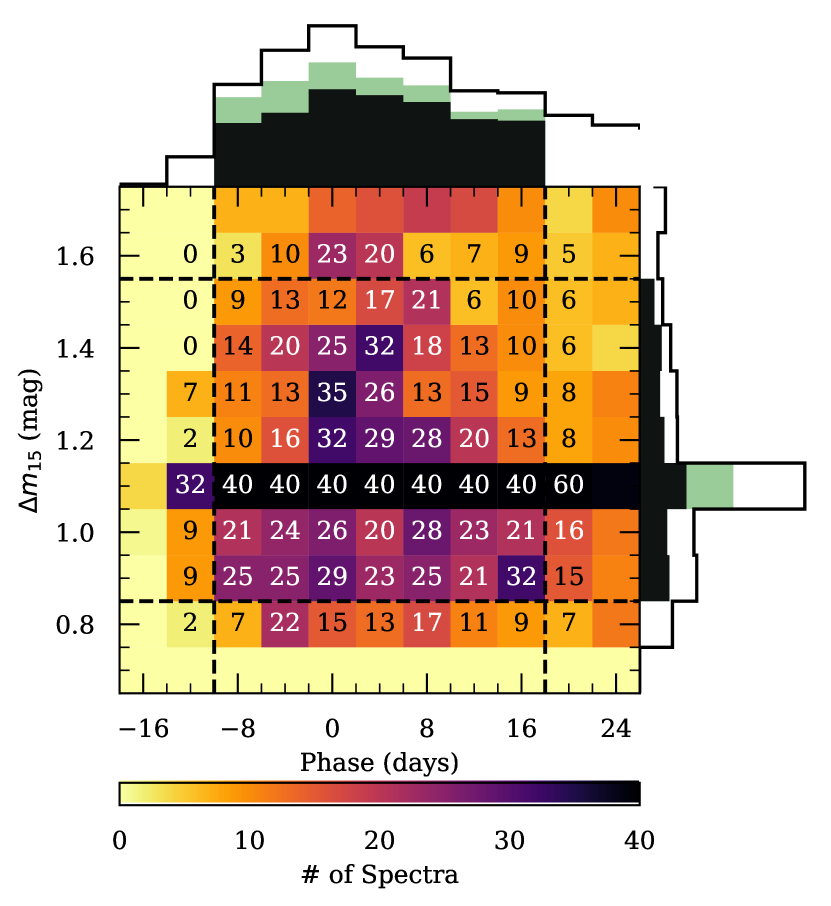
Figure 3: Distribution of $\Delta m_{15}$ and phase for the spectra in our compilation, with axes truncated to focus on the domain of interest. The empty-black one-dimensional projections reflect the full set of 3035 spectra, the green components consider only those 1394 spectra that are within the domain of interest, and the filled-black components show the same once spectra are removed to enforce the saturation criteria of 40 examples per bin (leaving 1113 in-domain spectra). The number of spectra falling within each in-domain bin and their immediate neighbors is labeled.

A cursory inspection of Figure 3 reveals that our coverage does not drop off significantly at larger phase and $\Delta m_{15}$ values than those which terminate our selected domain. It is therefore tempting to consider expanding the domain until such a drop is achieved (so as to make predictions over a wider swath of parameter space), but we choose not to do so for a myriad of reasons, the bulk of which are conveyed in the sequences of variance spectra presented in Figure 4. If we assume that the spectral energy distribution (SED) of a SN Ia is predominantly determined by its phase and light-curve shape, then considering sequences of variance spectra — whereby one of the aforementioned parameters is discretised into narrow bins and the variations within those bins are studied — allows us to infer which regions in SN Ia spectra vary the most at a given point in the sequence. If our assumption that the SED is largely a function of these two parameters holds, then such regions of large variation encode the most discriminating information about the nondiscretised parameter.

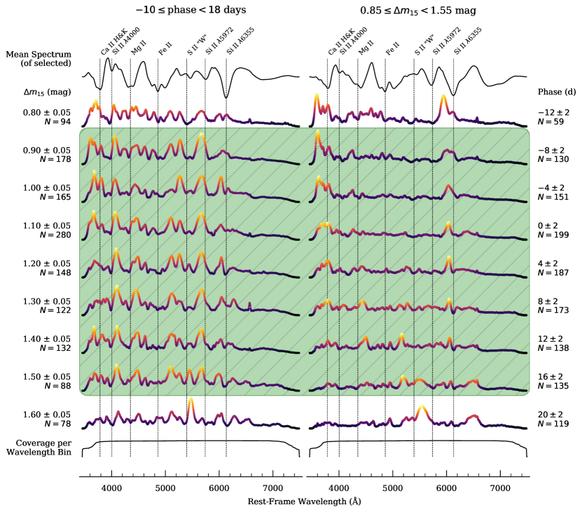
Figure 4: Sequences of variance spectra progressing through equally spaced $\Delta m_{15}$ (left column) and phase (right column) bins. Each column begins with the selection criteria for the spectra in it and the mean spectrum of all those that are selected. Prominent spectral features are indicated. After advancing through the indicated variance sequence, the column terminates with the coverage per wavelength bin of the selected spectra. The same vertical scaling is applied to all variance spectra, but the colour map is normalised to each and is used to emphasise regions of significant variation. Our selected domain of interest is covered by the green region with diagonal hatching. All spectra used in generating the sequences have been preprocessed according to the specifications of Section 2.3.2. The narrow spike that appears redward of the Si ii $\uplambda 6355$ line in some variance spectra is due to nebular H$\alpha$ emission from the host galaxy.

With this interpretation established, we note that for spectra with phases between $-10$ d and 18 d, the variance spectra in the left column of Figure 4 show notably similar structure for $\Delta m_{15}$ bins ranging from 0.90 mag to 1.50 mag. We interpret this as an indication that, at least within this range of $\Delta m_{15}$ values, phases between $-10$ d and 18 d are encoded by a common — or “slowly” evolving — set of features. A consequence of this is that a fairly simple convolutional neural network should be able to learn these features without much difficulty (we discuss our network architecture, including the way in which Figure 4 motives it, in more detail in Section 3.1), and although a sophisticated network may well be able to learn “when” to weight certain features more heavily — in addition to the features themselves — we are content with the range of $\Delta m_{15}$ values afforded by our selected domain. Indeed, our coverage drops off sharply for lower $\Delta m_{15}$ and the more rapidly declining SNe Ia in our dataset (i.e., those with $\Delta m_{15}\gtrsim 1.6$ mag) are likely to be SN 1991bg-like objects which do not follow the Phillips relation (or its derivatives).

The aforementioned arguments do not perfectly carry over when we consider the phase-binned variance spectra for those SNe Ia in our sample having $0.85\leq\Delta m_{15}<1.55$ mag. Before maximum light, the blue wing of the Ca ii H&K feature exhibits the most variability and thus offers the best discrimination of $\Delta m_{15}$, but beyond peak, this variability fades and the dominant variation is observed in the blue wing of the Si ii $\uplambda 6355$ feature. At phases $\gtrsim 10$ d, this too begins to fade and variability is strongest at intermediate wavelengths, typically those in the vicinity of the S ii “W” feature. It is beyond the scope of this study to speculate about — or offer an explanation of — the physical mechanism(s) that give rise to these observations, but we note that Nugent et al. (1995) identified these features in particular as a probe of SN Ia luminosity, with the cause ascribed to temperature differences (and thus, to the total amount of ⁵⁶Ni produced) between explosions. We do not pursue earlier phases owing to a paucity of data (indeed, Figure 3 reveals that doing so would result in several empty bins), and while our compilation may well support an extension to later phases, we do not undertake such an addition here because Model III would have to become very robust to evolving features.

2.3.1 Training, Validation, and Testing Sets

In developing a neural network (or any supervised ML model), one typically divides the available data into three distinct subsets: a “training” set used to derive the decision path between features and outputs, a “validation” set to assess model performance during training and tune externally assigned hyperparameters, and finally, a completely separate “testing” set, which is used to probe the efficacy of the final model against unseen data, and not used for either the optimisation of the network or the assignment of hyperparameters. In light of the small absolute size of our compilation (by modern ML standards), we intentionally set the validation and testing splits (10% each) to be smaller than conventional allocations so as to keep our training set as large as possible.

We take a nuanced approach to ensure that our proportionally smaller validation and testing sets provide a realistic representation of our final compilation. Specifically, we sample according to a pseudostratified scheme for the 1113 in-domain spectra in our compilation, whereby we select random subsets of the appropriate size from each bin in Figure 3. In this way, the Model II & III training, validation, and testing sets have approximately the same binwise distribution. We impose a floor so that even bins with fewer than 10 total instances have at least one sample for each of the validation and testing sets. As a result, the actual validation and testing ratios are elevated slightly higher than the targeted 10%. The Model I sets are generated by randomly sampling all out-of-domain spectra at the prescribed ratios and then adding them to the pseudostratified in-domain sets. This ensures that all spectra in the Model II/III sets are just subsets of the corresponding Model I sets. Therefore, we can holistically assess deepSIP via the Model I testing set without fear of Model II or III inadvertently being asked to characterise spectra that occur in their training or validation sets.

2.3.2 Preprocessing

Our models should be sensitive only to the physical characteristics encoded in the spectra they are trained on, not to any peculiarities relating to how the spectra were collected or reduced. Furthermore, it is imperative that each spectrum is processed in a carefully controlled and systematic way to avoid inadvertent biases. We therefore perform the following preprocessing steps to homogenise input spectra prior to ingestion by our models.

1. Each spectrum is de-redshifted — that is, the redshift is removed. This step is skipped for augmented spectra (see Section 2.3.3) which are already in (or near) the rest frame.

2. Each spectrum is smoothed using a Savitzky-Golay filter (Savitzky & Golay, 1964) with a window equivalent to 100 Å, though the window is varied for augmented spectra.

3. The pseudocontinuum is modeled by again smoothing the spectrum, but with a much wider window of 3000 Å (unless this exceeds the range of the spectrum, in which case we use a dynamically determined value corresponding to $\sim 70\%$ of the available wavelength range). We then subtract it from the spectrum.

4. The spectrum is binned onto a log-wavelength scale consisting of 1024 points between 3450 Å and 7500 Å. As shown in Figure 2, these endpoints are such that $\sim 50$% of our global compilation (i.e., including those without phase information) have additional spectral information either below 3450 Å or above 7500 Å that is disregarded. This painful step of throwing away potentially useful information is necessary to avoid inducing significant biases between our data sources. If a spectrum does not have signal all the way to the blue or red ends of this range, we set it to zero in the missing end(s). In addition to ensuring that all spectra are represented by vectors of the same length, this transformation has the useful consequence that redshifting corresponds to a linear translation (see Section 2.3.3 for more details).

5. We scale the signal so that it has a range of unity and then translate it such that it has a mean of zero.

6. The first and last 5% of the signal in the spectrum is tapered using a Cosine Bell (i.e., a Hanning window) so that it smoothly goes to zero at the ends.

7. Finally, we add 0.5 to the signal so that it is positive everywhere. Henceforth, we refer to this quantity as “scaled flux.”

We show an example of the intermediate stages and final result derived from our preprocessing procedure in Figure 5.

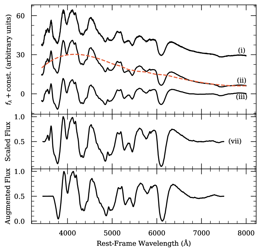
Figure 5: Snapshots showing various stages of our preprocessing routine as applied to a spectrum of SN 2016coj at $+1.3$ d. The numerals indicate the last preprocessing step to have been performed on the plotted spectrum, and the dashed orange line illustrates the fitted (and subsequently removed) pseudocontinuum. The bottom panel shows an example of the spectrum after data augmentation steps have been applied.

2.3.3 Augmentation

Though we have taken care to assemble a significant fraction of all publicly available low-redshift SN Ia optical spectra currently in existence, our final compilation is still rather small by modern standards in deep learning (especially for the domain-restricted subset that is relevant for Models II and III). For this reason, we formulate a data-augmentation strategy (i.e., a method for extending our training set beyond its limited size while preserving its characteristics; e.g., Dieleman et al., 2015; Cabrera-Vives et al., 2017; Martínez-Palomera et al., 2018; Boone, 2019) that generates a training set of substantially increased size. To accomplish this, we randomly sample data from the Model I (II/III) training set, with replacement, until we have a collection whose size, when combined with the non-augmented training set, equals 5000 examples (a $\sim 4$-to-1 ratio of augmented to original training samples for the Model II/III set). After obtaining samples according to this prescription, we transform each sampled spectrum using the following operations.

1. Redshifting: As noted in Section 2.3.2, we remove the redshift from all spectra that are fed into our models. However, we expect our models to be robust to small redshift errors that propagate into the rest-wavelength transformation. To this end, we perturb the rest wavelength array of each sampled spectrum by a multiplicative factor of $(1+\delta z)$, where $\delta z$ is drawn from a uniform distribution, $\delta z\sim\mathcal{U}(-0.004,0.004)$, motivated by the mean uncertainty in the SNID-derived redshifts reported by S20 for their dataset. Coupled with log-binning (which converts redshifting/de-redshifting into a linear offset; see Section 2.3.2), this allows us to reinforce and exploit the invariance to small translations that CNN architectures exhibit (LeCun et al., 2015).

2. Noise: To encourage our models to be robust to variations in the signal-to-noise ratios of input spectra, we vary the degree of smoothing applied to each sampled spectrum during our preprocessing procedures (see Section 5). We do this by randomly selecting the smoothing window, $w\sim\mathcal{U}(50,150)$ Å, with these bounds chosen to be roughly consistent with the range of wavelength-space extents of the high-variance regions identified in Figure 4.

3. Trimming: We expect our models to be insensitive to any information about the observing apparatus and configuration that might be encoded in a spectrum. For example, the median phase of the BSNIP-collected spectra in our compilation is $\sim 18$ d, while for the CfA-collected spectra it is $\sim 9$ d, but our models should not form a decision path that preferentially associates spectra having extensive red-wavelength coverage (namely, the BSNIP spectra) with later phases — this correlation is purely a consequence of exogenous biases in our compilation. Therefore, in addition to the preprocessing steps outlined in Section 2.3.2, we remove a random proportion, $f$, from the blue and red ends of each sampled spectrum, where $f\sim\mathcal{U}(0,0.1)$, with the upper bound chosen so as to maintain full coverage of the characteristic Si ii $\uplambda 6355$ feature that we require for spectra in our compilation to possess.

We show an example of the results of the aforementioned augmentation procedures in the bottom panel of Figure 5.

3 Models

As noted, we have constructed three models to ultimately determine the phase and light-curve shape parameter, $\Delta m_{15}$, of a SN Ia from an optical spectrum. The first model determines if the input is from a SN Ia with a phase of $-10\leq{\rm phase}<18$ d that has a light-curve-shape parameter of $0.85\leq\Delta m_{15}<1.55$ mag. The second model determines the phase, and the third, $\Delta m_{15}$, both only within the domain for which Model I discerns. We formulate the first model as a binary classification problem — either a spectrum belongs to a SN Ia subject to the aforementioned photometric restrictions, or it does not. The remaining models can be construed as a regression problem, where a continuous quantity (e.g., phase or $\Delta m_{15}$) is to be predicted. Despite their differing applications, each model uses a similar neural network architecture, and much of the work flow of training and evaluating them is common. We therefore devote the following subsections to discussing the underlying architecture employed in our models and the common aspects of our work flow. We present model-specific results in Section 4.

3.1 Architecture

At the heart of our models is a deep (i.e., multilayer) CNN, but whereas the prototypical use-case is two-dimensional (2D) — deep 2D CNNs have a storied history in image classification (e.g., LeCun et al., 1990; LeCun et al., 1998; Szegedy et al., 2014) and even Muthukrishna et al. (2019a) resorted to tiling 1D SN spectra into 2D “images” to formulate their problem as one of image identification — we follow the inherent dimensionality of our data by using a 1D implementation (for a summary of 1D CNNs, see Kiranyaz et al., 2019). In addition to being more conceptually compatible with our application, our use of a 1D CNN gives us much more control over the degree to which nonlocal features are aggregated though pooling operations.

We present a schematic of our neural architecture, which utilises a total of four convolutional layers to extract representative features from input spectra, in Figure 6. We apply the Rectified Linear Unit (ReLU, Nair & Hinton, 2010) activation function to the output of each convolutional and fully connected layer. Following each convolutional layer we apply max pooling to reduce computational complexity and remove irrelevant features. Finally, we conclude each “block” (i.e., convolution + ReLU + max pool + dropout) in our network with a dropout layer to assist in the prevention of overfitting (Srivastava et al., 2014). Each convolutional and fully connected layer has its weights initialised with zero-centred Gaussian noise and its bias to a small, positive value. All of our models are implemented using PyTorch 1.0 (Paszke et al., 2019), and we make our trained models and framework available as deepSIP, an open-source Python package (see Appendix C for guidelines on basic usage).

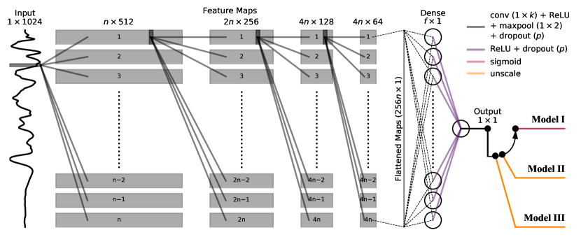
Figure 6: Schematic of the common neural network architecture used by each of the three fully independent networks that constitute Models I–III (which collectively comprise deepSIP). A set of $n$ feature maps is computed from the preprocessed input spectrum and down-sampled using max pooling (the resulting maps are indicated by grey boxes). This operation is then recursively applied to the down-sampled feature maps a total of three additional times, with the number of feature maps doubling for all but the last set. The final set of down-sampled feature maps is then flattened into a vector of length $256n$ and fed through a fully connected layer consisting of $f$ neurons before reaching the output neuron. Then, depending on the model, a final operation is performed to transform the raw output of the network into the appropriate context (“probabilities” in the case of Model I or dimensional phase or $\Delta m_{15}$ values for Models II and III, respectively). The convolution kernel, $k$, number of feature maps generated by the first convolutional layer, $n$, and the number of neurons in the fully-connected layer, $f$, are all hyperparameters whose preferred value depends on the specific model. A dropout layer with dropout probability $p$ follows each weight layer aside from the output neuron.

Our selected architecture is largely motivated by insights gleaned from the sequences of variance spectra presented in Figure 4. As noted earlier, the $\Delta m_{15}$-binned sequence shows more or less the same structure over our selected range of values. This homogeneity supports the use of a simple feed-forward network in the case of Model II, but the depth of the network (i.e., how many convolutional layers are used) and the progression in the number of filters computed per layer are motivated by the heterogeneity in features as they progress through the sequence. For example, the blue wing of the Si ii $\uplambda 6355$ feature shows variation throughout the sequence, but the exact “shape” of that variation as a function of wavelength varies. For this reason, we use multiple convolutional layers and increase the number of convolutional kernels per layer in all but the last so that our networks have the capacity to make decisions based on many complex, highly-specialised features that are computed from a smaller number of basic features supplied by the earlier layers. The situation is mostly the same for Model III, but the relevant variance spectra (i.e., those in the right column of Figure 4) exhibit fewer common features and more extreme evolution in their shapes as the sequence progresses through phase bins. Motivated by this, we did carry out experiments with several architectures capable of predicting the phase in tandem with $\Delta m_{15}$, but none performed substantively better than our set of simple, independent networks. We do expect, however, that in addition to requiring much more high-quality training data, a specialised architecture would be crucial in expanding the output domain of Models II and III. Indeed, extending the sequences of Figure 4 out to larger phase and $\Delta m_{15}$ values reveals significant feature evolution. A network capable of providing feedback between phase and $\Delta m_{15}$ predictions would allow for this evolution to be properly modeled.

The aforementioned dropout layers — each of which randomly drops elements from their input with Bernoulli-distributed probability, $p$, and (in our implementation) rescales outputs by a factor of $1/(1-p)$ during training — serve a secondary purpose in our networks. Namely, this purpose is to make the networks probabilistic (Gal & Ghahramani, 2015): each forward pass with dropout enabled in training mode produces a different prediction, and thus, it is straightforward to quantitatively describe not only a point estimate (the prediction of a model) but also, an estimate of its uncertainty. To do so when generating predictions, we make $N$ stochastic (i.e., with dropout turned on) forward passes for a given input and assign the mean and standard deviation of the resulting collection of predictions as the final model prediction and an estimate of its uncertainty.

3.2 Training

To train each of our models, we supply the appropriate training set in small batches and utilise an adaptive gradient descent algorithm (ADAM; Kingma & Ba, 2014) to minimise the appropriate objective function by updating the weights and biases in each layer of the network. For Model I we employ the binary cross-entropy loss as our objective function, while for Models II and III we use the mean squared error (MSE) loss. We also scale training outputs that are continuous (i.e., phase and $\Delta m_{15}$) such that they range from 0 to 1 using a transformation of the form $\mathbf{y}^{\prime}=(\mathbf{y}-y_{\rm min})/(y_{\rm max}-y_{\rm min})$, where $(y_{\rm min},y_{\rm max})$ represent the domain boundary (as shown in Figure 3) along the output’s dimension. Subsequent predictions by these models are then unscaled using the inverse of this transformation. Model I predictions are transformed into “probabilities” using the sigmoid function.

We train each of our models for a total of 75 epochs, with the learning rate set to step down by a multiplicative factor of 0.1 after thresholds of 45, 60, and 70 epochs are reached. In testing, we found these choices to yield stable convergences without requiring excessive training time. At the culmination of each epoch we compute success metrics against the relevant validation set, thereby affording a specific measure of model-performance evolution in terms of the metrics we care most about (e.g., in dimensional, unscaled units for Models II and III). For Model I, we primarily use the area under the curve (AUC) of the Receiver Operating Characteristic (ROC) curve, whereas for Models II and III, we primarily use the root-mean-square error (RMSE). We emphasise that although these are the primary metrics, we consider secondary indicators as well (see Sections 4.1 & 4.2 for Models I and II/III, respectively).

3.3 Hyperparameter Selection

There are several external parameters (i.e., not determined through backpropagation; henceforth referred to as “hyperparameters”) that must be selected specifically for each of our models. Some are architectural (e.g., $k$, the size of each convolutional kernel; $n$, the number of distinct feature maps computed by the first convolutional layer; $f$, the number of neurons in the fully-connected layer; and $p$, the dropout probability used for training; see Figure 6), and some have to do with our training algorithm (e.g., training batch size, learning rate, and weight decay). The optimal choice of such parameters is not known a priori and is application dependent (e.g., we find that Model II performs best when $k$ is less than the value that maximises Model III performance; see Table 1). We note that the dropout probability used during training need not be the same as that used when generating predictions. We therefore consider them separately as follows: the dropout probability for training is chosen as part of our hyperparameter selection process and the dropout probability used for generating predictions is separately chosen in tandem with $N$ (see Section 4.2.1).

Thus, for each of Models I, II, & III, we perform a randomised search whereby we select preferred hyperparameter values by training and validating the models on many combinations of hyperparameters that are randomly drawn from a grid. A total of 12 hr of compute time on a single of NVIDIA Tesla K80 GPU was allocated, per model, for these searches. We increase efficiency by automatically stopping training after 20 epochs when a performance threshold is not achieved on the validation set, and as a result, we are able to explore a significant portion of the selected hyperparameter space. Table 1 details the full hyperparameter grid, and summarises the final set for each model. We discuss our selection criteria for determining these final, preferred sets in Sections 4.1 & 4.2 for Models I and II/III, respectively.

Table 1: Hyperparameter Grid.

Hyperparameter	Valuesa
convolution kernelb ($k$)	$5,15,25^{{\rm I,II}},35^{{\rm III}}$
filters in first convolution ($n$)	$8^{{\rm I,II,III}},16,32$
fully connected neurons ($f$)	$16^{{\rm I,II}},32,64,128^{{\rm III}}$
training dropout probability ($p$)	$0.01^{{\rm I,II,III}},0.05,0.1$
batch sizec	$2,4,8,16^{{\rm I,II}},32^{{\rm III}}$
learning rate	$0.0005^{{\rm II,III}},0.001^{{\rm I}}$
weight decay	$0.00001^{{\rm III}},0.0001^{{\rm I,II}}$
aSuperscripts mark the preferred hyperparameter of the denoted model.
bThough small (e.g., $3\times 3$) kernels are typical in 2D scenarios, significantly larger kernels have proven optimal in some 1D applications to astrophysical signals (e.g., quasar spectra, Parks et al., 2018).
cMasters & Luschi (2018) have suggested that batch sizes between 2 and 32 yield the best performance.

4 Results

4.1 Model I: Domain Classification

4.1.1 Preferred Hyperparameters

Our first model is designed to determine if an input spectrum belongs to a SN Ia having $-10\leq{\rm phase}<18$ d and $0.85\leq\Delta m_{15}<1.55$ mag. If a spectrum satisfies these criteria, it is said to be in the domain of interest; otherwise it is out. In this way, Model I serves as a precursor to Models II and III: the subsequent predictions for spectra that it classifies as being outside the domain of interest should be carefully scrutinised, if not disregarded altogether. From our Model I hyperparameter search (as discussed in Section 3.3 and summarised in Table 1), we find that the highest achieved validation ROC AUC score is 0.992 (see Figure 7), and on the basis of this score, we select the hyperparameters that yield it as the final, preferred set. These hyperparameters produce a network with a relatively modest number ($\sim 75$k) of trainable parameters. Though we currently do not consider uncertainty estimates for Model I, we still use the full machinery of our probabilistic architecture with settings aligned to those of Models II and III (i.e., $N=30$ and $p=0.02$; see Section 4.2.1) for consistency and to grant straightforward extensibility in the future.

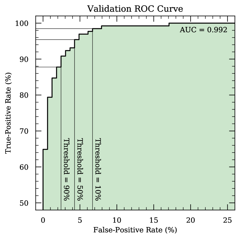
Figure 7: ROC curve for Model I deployed on its validation set. The locations that correspond to various decision thresholds are indicated.

4.1.2 Decision Threshold

With the information afforded by Figure 7, we are also able to tune the decision threshold of our model (i.e., the minimum “probability” of being in to be classified as such). While many opt to use a default threshold of 50% without further consideration, the optimal choice depends on striking an application-specific balance between the extent to which false positives can be tolerated and true positives can be missed. Taking a holistic view and recalling the aforementioned role of Model I in the overall output of deepSIP, it becomes obvious that the quality of Model II and III predictions should be given the utmost priority. The optimal decision threshold in our case is therefore the one that yields the best Model II and III performance on spectra that Model I classifies as in-domain (which will be a mixture of true positives and false positives). This criterion is much more important than the overall classification accuracy given the “blurry” nature of the domain boundary — individual spectra can and do fall so close to it that the particular side they end up on is determined by statistical variations.

To identify the optimal threshold, then, we use the Model I validation set to study, as a function of decision threshold, Model II/III RMSE scores segmented, based on the classifications of Model I, into false negatives (FN), false positives (FP), true positives (TP), and all positives (P = FP + TP). We find that the Model II scores belonging to FN and FP both follow a trend of decrease with rising decision threshold, and that those for FN are generally larger by a modest ($\sim 0.5$ d) amount. The corresponding FN scores for Model III also follow a decreasing trend (with rising threshold) but are significantly lower than those for the FP, which remain roughly constant at $\sim 0.2$ mag until a dip forms between $\sim 90$–95%. While one could argue that the FP scores for Model II are acceptable over a wide range of thresholds ($\sim 2$–2.5 d for thresholds of $\sim 5$–80%, and lower thereafter), the aforementioned Model III scores over a similar range are prohibitive. We simply cannot tolerate any significant contamination by FP with such high RMSE scores. This constrains the range of acceptable decision thresholds to just $\sim 90$–95%, even at the expense of more FN with reasonable Model II/III performance.

As the P scores are fairly flat between these bounds, we err to the low side (thereby minimising the number of incorrect classifications) and set our Model I decision threshold to 90%. This yields 13 FN (with RMSE scores of 1.91 d and 0.080 mag from Models II and III, respectively) and 122 P (with scores of 1.05 d and 0.068 mag, respectively) of which 4 are FP (with scores of 1.39 d and 0.160 mag, respectively) from the 295 spectra (including 160 true negatives) in our validation set. Though this results in an accuracy score ($94.2\%$) that is slightly suboptimal to the peak value of 95.9% achieved at a different threshold, it is still vastly in excess of the baseline score yielded by picking the most popular class every time ($55.6\%$) and it gives us confidence that the positives Model I passes on to Models II and III are sufficiently “pure.”

4.1.3 Performance on Testing Set

With the decision threshold determined, we now make predictions on the testing set (which, as outlined in Section 2.3.1, has not been used to optimise the network or hyperparameters) and assess the efficacy of Model I by comparing predicted labels to true labels. We find a similarly high ROC AUC of 0.989 and note that Model I achieves a TP rate of 90.8% at a FP rate of 2.4% for our selected threshold of 90%. From the 295 spectra in the testing set, Model I delivers 160 true negatives, 12 FN, 4 FP, and 119 TP, collectively yielding an accuracy score of 94.6% (as compared to the 55.6% baseline score obtained by picking the most popular class every time). Of those marked as in-domain (i.e., P), Models II and III yield RMSE scores of 1.06 d and 0.072 mag, respectively, while the TP subset performs even better at 1.00 d and 0.064 mag. These measures give us a high level of satisfaction with Model I, and we therefore consider it complete.

4.2 Models II & III: Photometric Quantity Estimation

4.2.1 Preferred Hyperparameters

Models II and III are intended to determine the rest-frame phase and $\Delta m_{15}$, respectively, of a SN Ia from its spectrum, assuming that it is within the phase and light-curve shape bounds that Model I identifies (i.e., the spectrum is in the relevant domain). As previously stated, our primary metric for regression tasks is the RMSE, but we consider two secondary indicators when selecting the final hyperparameter values: (i) the slope of a linear fit to predictions as a function of ground truth values, and (ii) the maximum absolute difference between predictions and labels (henceforth MR, for maximum residual). The first diagnoses the directionality of prediction errors — systematic overestimates for low values and underestimates for high values are conveyed in a fitted slope of less than unity (and vice versa, though our models only bias in the aforementioned direction; see Section 4.2.5), and the second gives an indication of how homogeneous the absolute residuals are (when compared with the corresponding RMSE score). It is not sufficient for a set of hyperparameters to yield a competitive RMSE score; they must yield competitive scores across each of these three metrics.

We therefore identify the preferred hyperparameters for Models II and III using a tiered approach to our search results. First, we filter to select only those results that have a slope above and an MR below a fiducial value when evaluated against the relevant validation set. Then, from the resulting subset, we select the entry with the lowest RMSE score. In this way, the final, preferred Model II hyperparameters are chosen for yielding an RMSE of 1.15 d, a slope of 0.96, and an MR of 4.32 d and the Model III hyperparameters on the basis of yielding scores of 0.065 mag, 0.823, and 0.206 mag, respectively. The final networks have $\sim 75$k and $\sim 320$k trainable parameters, respectively. Although it is beyond the scope of this study to make any definitive or in-depth statements about the significance of the final hyperparameters, it is interesting to note the differences between those that yield the best observed performance in Models II and III. For example, we find that Model III performs best with a larger convolution kernel, $k$, than does Model II (35 for Model III versus 25 for Model II); this may indicate that features encoding phase information are generally narrower than those which encode $\Delta m_{15}$. At the same time, Model II requires fewer neurons in the fully connected layer than does Model III. This is consistent with our general intuition that phases are more “simply” codified in spectral features than $\Delta m_{15}$ (or other luminosity indicators), which may be best parameterised by ratios of nonlocal features (as suggested by Nugent et al., 1995).

As a final refinement to the parameters that govern Models II and III, we study the effect of varying the number of stochastic forward passes ($N$) and dropout probability ($p$) when the models are used to generate predictions. To do so, we use Models II and III to generate predictions from the relevant validation set over a grid of $(N,p)$ values and then tabulate the RMSE and mean estimated uncertainty at each point. The results (visualised in Figure 8) are generally consistent with our expectations: mean predicted uncertainties steadily grow with $p$ as do RMSE values, albeit at a much less significant rate. For Model III, both metrics show minimal dependence on $N$, but for Model II there are “bands” of improved RMSE performance at $N=30$–80, 140–160, and beyond 180 (though they only outperform their surroundings by $\lesssim 0.2$ d). While our primary concern is optimising model performance (i.e., achieving low RMSE scores and “reasonable” uncertainty estimates), it is desirable from a compute-time perspective to use the lowest $N$ value possible. We therefore select $(N,p)=(30,0.02)$ for all deepSIP predictions. As Figure 8 clearly shows, this yields the desired low $N$ (for fast prediction times) without compromising the quality of model predictions.

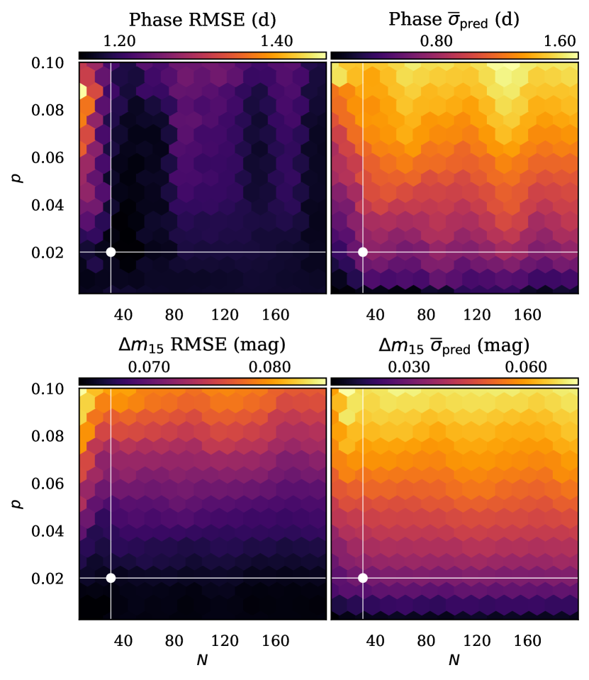
Figure 8: Validation RMSE and mean predicted uncertainty values for Models II and III over a grid of $N$ and $p$ values. A separate colour bar is provided for each panel, and the selected $(N,p)$ set is indicated.

4.2.2 Performance on Testing Set

Having selected the final hyperparameters for each model, we make predictions on the relevant testing sets. As shown in Figure 9, we find strong agreement when we compare predictions to ground truth labels, achieving RMSE, slope, and MR scores of 1.00 d, 0.97, and 3.22 d; and 0.068 mag, 0.809, and 0.228 mag, respectively. For the 131 samples in each testing set, the median phase ($\Delta m_{15}$) residual is $-0.19$ d ($0.001$ mag); also, 94 (94) are within one standard deviation of the median, 122 (123) are within two, and 130 (129) are within three.

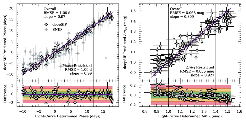
Figure 9: Phase (left panel) and $\Delta m_{15}$ (right panel) determined by deepSIP versus ground truth values from the respective Model II and III testing sets, with residuals in the lower panels. The indigo line in each upper plot shows the one-to-one correspondence for ground truth values, while in the lower plots, it indicates the median residual. The green, yellow, and red regions indicate the $1\sigma,2\sigma$, and $3\sigma$ bounds about the median residual, respectively. We mark the relevant RSME and slope, both globally and for a restricted subset (see Section 4.2.5) in each panel. SNID-based phase predictions are presented as an overlay to the upper-left panel, but they are omitted from the residuals for clarity.

In Section 4.2.6, we investigate the quality of the uncertainty estimates produced by our models, which serve as a systematic error probe by quantifying the dispersion between $N$ realisations drawn (for each input spectrum) from the underlying distribution that is each of our models. Here we do the opposite in an attempt to quantify statistical error: we remove the stochasticity from our models (by disabling dropout) and assess prediction robustness when they are fed perturbed inputs. We generate such inputs using our data-augmentation strategy (see Section 2.3.3) to bootstrap our Model II and III testing sets up to 5000 instances, each of which is slightly perturbed in redshift, noise, and signal length. The results, which we assess by means of the RMSE, are highly satisfactory: Model II yields 1.05 d and Model III delivers 0.080 mag, both broadly consistent with the corresponding measures reported above. One could potentially use a variation of this strategy to generate a unique statistical uncertainty estimate for each input spectrum and include that with each prediction, but we defer that task to future study and development.

4.2.3 Comparison with SNID-derived Phases

To contextualise the level of performance of Model II with regard to phase predictions, we attempt to characterise the spectra in the testing set using a series of SNID runs that adhere to the specifications laid out by S20. When we do so, we find that deepSIP performs significantly better than SNID in virtually every way. Whereas the SNID-based scheme (consisting of a total of four runs per spectrum, all of which are controlled and read using a Python script and hence subject to small Python overheads) takes $\sim 7$ min to process all 131 testing samples on a server with a modern CPU, our Model II (which entails a total of 30 stochastic forward passes per spectrum) takes under 1 s on a single NVIDIA Tesla K80 GPU to characterise preprocessed spectra ($<1$ min on a modern, four-core CPU), with $<1$ s for preprocessing. Moreover, the SNID approach fails to derive a phase in 18/131 instances while deepSIP is successful in making a prediction in all cases. Perhaps most significantly, the RMSE between those instances where SNID successfully predicts a phase and the true phases is $3.48$ d, a factor of $\sim 3.5$ times worse (in RMSE; $\sim 12$ times worse in MSE) than that for our deepSIP-derived results. The SNID results are also much more afflicted by a bias to overestimate the earliest phases (a tendency that has been observed and discussed by S20 and others); the mean residual (predicted minus true) at phases from $-10$ d to $-5$ d is $+3.30$ d for SNID-derived results, but just $+0.31$ d for those from deepSIP. This bias is also exhibited in the aforementioned fitted-slope metric, with SNID yielding a value of 0.80 compared to 0.97 for Model II.

4.2.4 $\Delta m_{15}$ Consistency

Unfortunately, we are unable to perform an analogous SNID-based comparison for $\Delta m_{15}$ values, but we can exploit a unique feature that the $\Delta m_{15}$ labels possess to perform a separate test on the validity of Model III. Unlike phases which are are unique to individual spectra, $\Delta m_{15}$ values are unique to individual SNe Ia. As a result, it is not uncommon for multiple spectra in the training, validation, or testing sets to map to the same $\Delta m_{15}$ value. We can test how well Model III deals with this degeneracy by looking at the scatter (parameterised by the standard deviation) in $\Delta m_{15}$ predictions in the testing set, grouped by distinct $\Delta m_{15}$ label (and therefore, by distinct object).

When we do so, we find encouraging results which we summarise with the following observations: (i) as compared to the global scatter in predicted $\Delta m_{15}$ values (0.161 mag), the median scatter in predicted values per distinct $\Delta m_{15}$ label is just 0.018 mag; (ii) the observed distribution is positively skewed so that the majority of the scatter is near zero (e.g., the 25th percentile is 0.007 mag while the 75th percentile is 0.045 mag); and (iii) of the two examples with scatter $>0.07$ mag, both are at or near the extremes of the predicted $\Delta m_{15}$ values (i.e., where the model’s predictions are typically the most uncertain and the training data are sparsest).

4.2.5 Biases

Though mitigated by our selection criteria (namely, our choice to enforce a 40 spectrum-per-bin saturation policy), Model II and (especially) Model III do exhibit some bias toward the more central values in their prediction ranges. This is unfortunate, but expected given the nonuniformity of our training data (e.g., see Figures 3 & 10). We emphasise that despite this bias, the residual distributions are approximately symmetric. Still, it is useful to quantify the extent of this bias, and we choose to do so by means of the previously mentioned slope of a linear fit to the results presented in Figure 9.

In doing so, we find a slope of 0.97 for phases and 0.809 for $\Delta m_{15}$ values, confirming our suspicion that the bias is present (and more pronounced in Model III). However, if we select a more restrictive subset to exclude the biased ends (taken to be the equivalent of 1.5 bins from Figure 3; i.e., 6 d and 0.15 mag from each end), the fitted slopes improve to 0.99 and 0.927, respectively. The Model III RMSE value improves as well, dropping to 0.056 mag. Users of deepSIP may therefore choose to give more weight to results within these restricted ranges. Such improvements reinforce our belief that more performance could be extracted from our models with a larger and more balanced training set.

4.2.6 Estimated Uncertainties

The aforementioned metrics are quite satisfactory, but we must also verify the quality of the uncertainty estimates produced by our models. A basic measure of this is afforded by comparing RMSE to weighted RMSE values (henceforth, wRMSE), defined by

$${\rm wRMSE}=\sqrt{\frac{\sum_{i=1}^{N}(\hat{y}_{i}-y_{i})^{2}\hat{\sigma}^{-2}_{i}}{\sum_{i=1}^{N}\hat{\sigma}^{-2}_{i}}},$$ (1)

where $\mathbf{y}$ are ground truth labels, and $(\mathbf{\hat{y}},\hat{\sigma})$ are the corresponding predicted labels and estimated uncertainties (i.e., the mean and standard deviation of the stochastic samples generated as described in Section 3.1). A situation where wRMSE $>$ RMSE would reflect poorly on the uncertainty estimates because it would imply, in aggregate, an inverse correlation between them and residuals (i.e., model predictions are generally more wrong where the model is more certain); conversely, a situation where wRMSE $<$ RMSE is an affirmation (but not conclusive determination) of the quality of our uncertainty estimates because it suggests that model predictions are generally more correct where the model is more certain. In our case, the results are favorable (albeit at only a modest level): Model II yields a wRMSE score of 0.92 d while Model III yields 0.065 mag.

To further probe the quality of our estimated uncertainties, one might be tempted to study the relationship between estimated and true uncertainties (i.e., those derived from light-curve fits). This, however, would not be appropriate because the true uncertainties were not accounted for by our loss function during model training (nor anywhere else aside from selection cuts). Instead, we can ask a more appropriate question of our estimated uncertainties: how do they behave relative to the data our models were trained on? The answer, depicted in Figure 10, is encouraging. We see that our estimated uncertainties for both models are generally smallest in the region where training data are most abundant, and that the uncertainties grow steadily as the training data become more scarce. This captures the general behaviour we desire, though the uncertainties may be modestly underestimated (given the lower panels in Figure 9, but we defer an extensive study of this to future work). Thus, on the basis of this desired behaviour and all prior points elucidated above, we consider Models II and III ready for deployment.

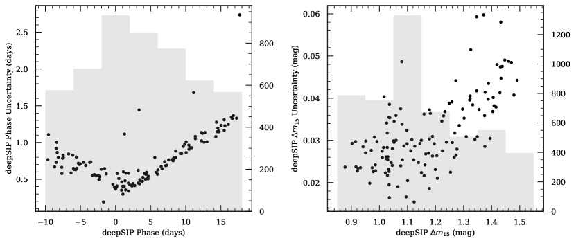
Figure 10: deepSIP-determined phase (left panel) and $\Delta m_{15}$ (right panel) uncertainties versus predicted values from the respective Model II and III testing sets. The grey distributions behind each convey the relevant training data (including those from the augmented training set).

5 Conclusion

In this paper we present and characterise the performance of deepSIP, an open-source software package that encapsulates a set of three CNNs that collectively map optical SN Ia spectra to their corresponding phases and light-curve shapes (parameterised by $\Delta m_{15}$). The treatment of these tasks with supervised learning — and the specific use of a CNN architecture — is a natural choice in many regards. This choice is rewarded with highly satisfactory performance.

To train, validate, and test our models, we compile a significant collection of low-redshift SN Ia spectra by drawing from public data releases from the CfA, CSP, and our own BSNIP. These spectra form, after preprocessing, the inputs of the input-output pairs that our models learn to map. To assemble the corresponding outputs (i.e., phases and light-curve shapes), we draw from the photometric data releases of the same research campaigns, supplementing with five SNe Ia for which we publish light curves that have recently become available in our own archives. We fit all light curves (except for those from S19 and CSP3 who performed the same fits) using the SNooPy $E(B-V)$ model, ensuring systematic consistency between all phase and $\Delta m_{15}$ values used herein. After all cuts are accounted for, our final compilation consists of 2754 spectra with photometrically-derived phase and $\Delta m_{15}$ values, and of these, 1113 are within the phase and $\Delta m_{15}$ constrained domain of interest for Models II and III.

Because we draw spectra from multiple sources, we take great care to both understand and mitigate systematic differences between sources so that our models form decision paths exclusively from physically significant features encoded in the spectra. Our mitigation strategy manifests chiefly in our preprocessing procedure which, among other things, discards any spectral information below 3450 Å  or above 7500 Å. Though painful, this prevents our models from being affected by the presence or absence of signal at more extreme wavelengths — a distinction which on the red end almost perfectly segments CfA, CSP, and BSNIP spectra. We also let our desire for telescope agnosticism guide the data augmentation strategy that we employ to increase our modest sample size. In addition to a redshift perturbation, we vary the extent to which augmented spectra are smoothed and randomly drop signal from the ends. The latter two actions serve to blur out the signature imparted by the specific equipment used to collect a given spectrum.

We describe the common neural network architecture which underlies each of our models and whose organisation and layout is largely motivated by our consideration of sequences of variance spectra. Under the assumption that spectral variations in SNe Ia are mostly a result of phase and light-curve shape (i.e., luminosity, via a width-luminosity relation), such sequences inform us about which regions in spectra most strongly encode a given target. Our observation of a relatively consistent set of features in such sequences has informed our adoption of a rather simple feed-forward network. To estimate uncertainties alongside point values for our targets, we use a probabilistic model provided by dropout variational inference. We employ a randomised grid search to determine the preferred set of hyperparameters for each of Models I–III, and upon doing so, set out to assess their performance.

To do so, we deploy each model against a distinct (i.e., unused during training and hyperparameter selection) testing set. In the case of Model I (a binary classifier of “in/out” with regard to a domain defined by $-10\leq{\rm phase}<18$ d and $0.85\leq\Delta m_{15}<1.55$ mag), we achieve an accuracy score of 94.6% and ROC AUC of 0.989. At a false-positive rate of 2.4%, Model I has an in-domain detection rate of 90.8%. With Model II (a continuous predictor of phases from $-10$ d to 18 d), we achieve an RMSE (wRMSE) of 1.00 d (0.92 d), a marked improvement over SNID-derived predictions on the same spectra. Finally, for Model III (a continuous predictor of $\Delta m_{15}$ values from 0.85 mag to 1.55 mag), we achieve an RMSE (wRMSE) of 0.068 mag (0.065 mag). These final, trained models are publicly available through deepSIP which provides an easy-to-use API for deploying them to characterise new SN Ia spectra. We strongly encourage public use of deepSIP for this purpose.

Looking to the future, we expect that the performance of deepSIP could be significantly improved as more spectra with corresponding light curves become available. Indeed, the dominant factor in our selection of the phase–$\Delta m_{15}$ domain inside of which Models II and III offer predictions is the paucity of data available with more extreme light-curve shapes. As such data become more prevalent, the networks which underly deepSIP can easily be retrained and if necessary, modified to accommodate feedback between predicted phase and $\Delta m_{15}$ values that may be necessary given the substantial feature evolution observed beyond the domain boundary. We welcome community involvement on these fronts (accumulating more data and designing more sophisticated network architectures), and intend to continue active, transparent development on our publicly hosted GitHub repository.

Data Availability

The data published herein are available in the article and in its online supplementary material.

Appendix A Supplementary Light Curves

In the time since the photometric dataset presented by S19 was published, we have continued to obtain host-galaxy template images for the unpublished SNe Ia in our archives. With these new observations, we are able to process five additional SNe Ia (SN 2007S, SN 2008hv, SN 2010kg, SN 2017hpa, and SN 2018oh.) of utility to this work. We therefore present their BVRI light curves (some also have unfiltered observations, which we refer to as Clear). All processing steps are identical to those described by S19, so we provide only a brief summary of the methodology before delivering results.

All images were collected using either the 0.76 m Katzman Automatic Imaging Telescope (KAIT; Li et al., 2000; Filippenko et al., 2001) or the 1 m Nickel telescope, both of which are located at Lick Observatory where the seeing averages $\sim 2^{\prime\prime}$. After removing bias and dark current, flat-field correcting, and deriving an astrometric solution, we pass images to our automated photometry pipeline (LOSSPhotPypeline; see S19), which handles all aspects of the remaining processing.

With host-galaxy template images obtained on dark nights using the Nickel telescope, the pipeline removes contaminating flux due to a SN’s host galaxy and then performs point-spread function (PSF) photometry using procedures from the IDL Astronomy User’s Library to measure the SN’s flux relative to selected standard stars in the same field. The resulting instrumental magnitudes are calibrated with at least two (but often more) of the selected standard stars from the Pan-STARRS1 Survey (PS1; Chambers & Pan-STARRS Team, 2018). To do this, PS1 magnitudes are transformed to the Landolt (1992) system using the prescription given by Tonry et al. (2012), and then into the appropriate natural-system magnitudes using coupled equations of the form

$$b =B+C_{B}(B-V)+{\rm constant},$$ (2)

$$v =V+C_{V}(B-V)+{\rm constant},$$ (3)

$$r =R+C_{R}(V-R)+{\rm constant,and}$$ (4)

$$i =I+C_{I}(V-I)+{\rm constant},$$ (5)

where natural (Landolt) system magnitudes are expressed in lower (upper)-case letters and $C_{X}$ is the linear colour term corresponding to filter $X$ (given in S19’s Table 1). Temporally close ($<0.4$ d) observations in the same passband are averaged together and then those in distinct passbands are grouped by their midpoint epoch to form natural-system light curves. Finally, the aforementioned equations are inverted to yield standardised light curves on the Landolt system. The uncertainties on each magnitude in our light curves are ultimately derived from three sources: “statistical” (e.g., Poisson variations in observed brightness, scatter in sky values, uncertainty in sky brightness), “calibration” (e.g., derived colour terms, uncertainty in PS1 magnitudes), and “simulation” (as described by S19).

We present the final Landolt-system light curves derived from the aforementioned processing steps in Figure 11. The final light curves are publicly available through our U.C. Berkeley SuperNova DataBase (SNDB; S12; Shivvers et al., 2016) and in the Supplementary Materials included with this article. We describe our method for (and results from) fitting these light curves (and the others in our compilation) using SNooPy in the following section.

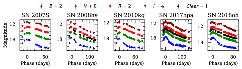
Figure 11: Observed light curves for the previously unpublished SNe Ia in our archives. In most cases the error bars are smaller than the points themselves. All dates have been shifted relative to the time of maximum B-band brightness. The light curves are available in tabular form through our SNDB and are also accessible as online supplementary material.

Appendix B Light-Curve Fitting

We use the $E(B-V)$ model as implemented by the SNooPy package to simultaneously fit the BVRI (or subset thereof) light curves in our photometry compilation. The model assumes a peak B-band magnitude and $B-X$ colours parameterised by the decline rate, and the results from fitting are the time of maximum B-band light ($t_{\rm max}$), decline-rate parameter ($\Delta m_{15}$), host-galaxy reddening, and distance modulus. We use the fitting results obtained by S19 and CSP for their datasets, and employ the strategy of the former to fit the remaining SNe Ia in our photometry compilation (i.e., those from G10 and CfA1-3). We give the resulting values of $t_{\rm max}$ and $\Delta m_{15}$ for all SNe which pass a visual inspection for fit quality in Table LABEL:tab:snoopy-fits, and defer a more thorough explanation of the fitting process to S19 (and their listed references).

Table 2: SNooPy Fitted Parameters.

SN	Sourcea	$t_{\rm max}$ (MJD)	$\Delta m_{15}$ (mag)	SN	Sourcea	$t_{\rm max}$ (MJD)	$\Delta m_{15}$ (mag)	SN	Sourcea	$t_{\rm max}$ (MJD)	$\Delta m_{15}$ (mag)
1993ac	CfA1	$49269.34\pm 0.70$	$1.098\pm 0.040$	2001bg	G10	$52039.95\pm 0.24$	$1.155\pm 0.029$	2004dt	G10	$53240.19\pm 0.18$	$1.136\pm 0.022$
1993ae	CfA1	$49289.15\pm 0.19$	$1.480\pm 0.022$	2001br	G10	$52051.78\pm 0.16$	$1.435\pm 0.024$	2004fu	CfA3	$53325.28\pm 0.48$	$1.170\pm 0.063$
1994M	CfA1	$49474.56\pm 0.29$	$1.331\pm 0.021$	2001cj	G10	$52064.98\pm 0.11$	$0.903\pm 0.013$	2004fz	G10	$53333.53\pm 0.10$	$1.473\pm 0.027$
1994Q	CfA1	$49495.35\pm 0.40$	$1.093\pm 0.020$	2001ck	G10	$52072.10\pm 0.12$	$1.079\pm 0.017$	2005bc	G10	$53469.96\pm 0.12$	$1.646\pm 0.028$
1994S	CfA1	$49517.90\pm 0.36$	$1.021\pm 0.038$	2001cp	G10	$52087.82\pm 0.08$	$0.884\pm 0.009$	2005bo	G10	$53478.10\pm 0.16$	$1.270\pm 0.008$
1994ae	CfA1	$49685.19\pm 0.10$	$1.058\pm 0.011$	2001da	G10	$52107.02\pm 0.19$	$1.149\pm 0.021$	2005cf	G10	$53533.85\pm 0.08$	$1.123\pm 0.008$
1995D	CfA1	$49767.78\pm 0.16$	$0.886\pm 0.012$	2001dl	G10	$52130.58\pm 0.12$	$1.022\pm 0.023$	2005de	G10	$53598.65\pm 0.10$	$1.216\pm 0.012$
1995E	CfA1	$49774.49\pm 0.22$	$1.069\pm 0.018$	2001eh	G10	$52168.42\pm 0.16$	$0.837\pm 0.006$	2005eu	G10	$53659.81\pm 0.12$	$1.099\pm 0.018$
1995ac	CfA1	$49992.44\pm 0.30$	$0.941\pm 0.036$	2001en	G10	$52192.43\pm 0.10$	$1.282\pm 0.005$	2005hf	CfA3	$53660.68\pm 0.95$	$1.449\pm 0.053$
1995ak	CfA1	$50022.22\pm 0.50$	$1.278\pm 0.018$	2001ep	G10	$52199.65\pm 0.17$	$1.133\pm 0.023$	2005ls	CfA3	$53714.40\pm 0.31$	$0.930\pm 0.033$
1995al	CfA1	$50028.26\pm 0.19$	$0.910\pm 0.014$	2001ex	G10	$52204.27\pm 0.28$	$1.813\pm 0.029$	2005lz	CfA3	$53735.82\pm 0.39$	$1.276\pm 0.031$
1995bd	CfA1	$50086.33\pm 0.15$	$0.937\pm 0.030$	2001fe	CfA3	$52229.01\pm 0.30$	$0.956\pm 0.019$	2005mc	CfA3	$53733.83\pm 0.22$	$1.733\pm 0.026$
1996C	CfA1	$50127.77\pm 0.33$	$0.965\pm 0.019$	2002G	G10	$52297.43\pm 0.43$	$1.145\pm 0.050$	2005ms	CfA3	$53744.16\pm 0.10$	$1.079\pm 0.018$
1996X	CfA1	$50190.73\pm 0.13$	$1.225\pm 0.009$	2002aw	G10	$52324.57\pm 0.25$	$1.123\pm 0.017$	2005mz	CfA3	$53745.01\pm 0.13$	$1.864\pm 0.003$
1996ai	CfA1	$50256.52\pm 0.38$	$1.112\pm 0.036$	2002bf	G10	$52335.09\pm 0.00$	$1.093\pm 0.032$	2006X	G10	$53786.01\pm 0.55$	$0.971\pm 0.038$
1996bk	CfA1	$50369.07\pm 0.55$	$1.758\pm 0.010$	2002bo	G10	$52356.29\pm 0.12$	$1.105\pm 0.014$	2006ac	G10	$53779.74\pm 0.51$	$1.199\pm 0.029$
1996bl	CfA1	$50376.23\pm 0.19$	$1.100\pm 0.019$	2002bz	CfA3	$52368.19\pm 0.53$	$1.366\pm 0.045$	2006al	CfA3	$53789.06\pm 0.35$	$1.569\pm 0.044$
1996bo	CfA1	$50386.51\pm 0.38$	$1.156\pm 0.036$	2002cd	G10	$52384.39\pm 0.23$	$1.101\pm 0.024$	2006az	CfA3	$53826.76\pm 0.13$	$1.354\pm 0.027$
1996bv	CfA1	$50403.42\pm 0.39$	$0.930\pm 0.023$	2002cf	G10	$52384.39\pm 0.10$	$1.823\pm 0.001$	2006bb	CfA3	$53815.83\pm 0.48$	$1.615\pm 0.018$
1997bp	CfA2	$50550.08\pm 0.43$	$1.114\pm 0.049$	2002cr	G10	$52409.07\pm 0.09$	$1.260\pm 0.007$	2006bt	G10	$53857.71\pm 0.23$	$1.091\pm 0.036$
1997bq	CfA2	$50558.43\pm 0.31$	$1.136\pm 0.031$	2002cs	G10	$52410.26\pm 0.17$	$1.097\pm 0.020$	2006cc	CfA3	$53874.13\pm 0.13$	$1.044\pm 0.030$
1997br	CfA2	$50559.90\pm 0.27$	$1.122\pm 0.027$	2002cu	G10	$52416.12\pm 0.10$	$1.461\pm 0.022$	2006cp	G10	$53896.91\pm 0.31$	$1.130\pm 0.054$
1997cw	CfA2	$50627.98\pm 0.44$	$0.811\pm 0.020$	2002de	G10	$52432.99\pm 0.16$	$1.071\pm 0.021$	2006dm	G10	$53928.20\pm 0.09$	$1.523\pm 0.017$
1997do	CfA2	$50766.18\pm 0.23$	$1.088\pm 0.023$	2002dj	G10	$52450.79\pm 0.35$	$1.149\pm 0.046$	2006ef	G10	$53968.14\pm 0.22$	$1.273\pm 0.012$
1997dt	CfA2	$50786.77\pm 0.23$	$1.341\pm 0.054$	2002dl	G10	$52451.92\pm 0.09$	$1.759\pm 0.007$	2006ej	G10	$53975.67\pm 0.17$	$1.498\pm 0.037$
1998ab	CfA2	$50914.39\pm 0.19$	$1.103\pm 0.021$	2002do	G10	$52441.42\pm 0.47$	$1.718\pm 0.010$	2006em	G10	$53976.32\pm 0.24$	$1.823\pm 0.001$
1998bp	CfA2	$50936.36\pm 0.18$	$1.800\pm 0.012$	2002dp	G10	$52450.38\pm 0.11$	$1.214\pm 0.008$	2006en	G10	$53970.97\pm 0.34$	$0.974\pm 0.021$
1998de	G10	$51025.70\pm 0.12$	$1.821\pm 0.001$	2002eb	G10	$52494.31\pm 0.08$	$1.067\pm 0.012$	2006gr	G10	$54012.41\pm 0.13$	$1.084\pm 0.017$
1998dh	G10	$51029.00\pm 0.12$	$1.118\pm 0.015$	2002ef	G10	$52489.88\pm 0.17$	$1.144\pm 0.019$	2006hb	G10	$54000.62\pm 0.29$	$1.693\pm 0.011$
1998dk	CfA2	$51057.17\pm 0.29$	$1.135\pm 0.015$	2002el	G10	$52507.93\pm 0.07$	$1.367\pm 0.020$	2006le	G10	$54047.74\pm 0.16$	$1.082\pm 0.018$
1998dm	G10	$51060.25\pm 0.12$	$1.008\pm 0.015$	2002er	G10	$52524.49\pm 0.16$	$1.140\pm 0.018$	2006lf	G10	$54045.03\pm 0.17$	$1.459\pm 0.032$
1998ec	G10	$51088.65\pm 0.93$	$1.146\pm 0.072$	2002eu	G10	$52520.22\pm 0.24$	$1.731\pm 0.010$	2006mo	CfA3	$54048.02\pm 0.35$	$1.653\pm 0.047$
1998ef	G10	$51113.19\pm 0.10$	$1.280\pm 0.007$	2002fb	G10	$52529.02\pm 0.09$	$1.824\pm 0.000$	2006mp	CfA3	$54053.92\pm 0.12$	$0.995\pm 0.019$
1998eg	G10	$51110.13\pm 0.70$	$1.117\pm 0.047$	2002fk	G10	$52547.13\pm 0.10$	$1.027\pm 0.010$	2006oa	CfA3	$54066.52\pm 0.19$	$0.953\pm 0.054$
1998es	G10	$51142.61\pm 0.07$	$0.925\pm 0.010$	2002ha	G10	$52580.77\pm 0.04$	$1.362\pm 0.008$	2006qo	CfA3	$54082.94\pm 0.15$	$1.054\pm 0.014$
1999aa	G10	$51231.89\pm 0.13$	$0.886\pm 0.014$	2002he	G10	$52585.40\pm 0.06$	$1.439\pm 0.011$	2006sr	CfA3	$54092.38\pm 0.14$	$1.279\pm 0.011$
1999ac	G10	$51249.98\pm 0.19$	$1.104\pm 0.022$	2002hu	CfA3	$52592.12\pm 0.13$	$1.089\pm 0.015$	2006td	CfA3	$54099.32\pm 0.14$	$1.422\pm 0.020$
1999by	G10	$51307.95\pm 0.10$	$1.824\pm 0.000$	2002hw	CfA3	$52595.63\pm 0.12$	$1.552\pm 0.027$	2006te	CfA3	$54096.89\pm 0.40$	$1.130\pm 0.021$
1999cc	CfA2	$51315.33\pm 0.18$	$1.344\pm 0.028$	2002jg	G10	$52609.62\pm 0.07$	$1.417\pm 0.019$	2007O	G10	$54122.77\pm 0.40$	$1.139\pm 0.041$
1999cl	G10	$51340.88\pm 0.22$	$1.144\pm 0.026$	2002jy	CfA3	$52634.02\pm 0.37$	$0.881\pm 0.026$	2007S	this	$54144.73\pm 0.24$	$0.836\pm 0.005$
1999cp	G10	$51362.61\pm 0.12$	$1.032\pm 0.021$	2002kf	CfA3	$52638.27\pm 0.43$	$1.236\pm 0.016$	2007al	CfA3	$54169.59\pm 0.25$	$1.857\pm 0.016$
1999da	G10	$51369.79\pm 0.09$	$1.823\pm 0.001$	2003W	G10	$52679.65\pm 0.23$	$1.130\pm 0.029$	2007ap	CfA3	$54168.31\pm 0.15$	$1.490\pm 0.018$
1999dg	G10	$51392.64\pm 0.32$	$1.509\pm 0.049$	2003Y	G10	$52676.54\pm 0.12$	$1.822\pm 0.001$	2007au	G10	$54183.75\pm 0.17$	$1.754\pm 0.017$
1999dk	G10	$51414.72\pm 0.13$	$1.103\pm 0.014$	2003cg	G10	$52729.24\pm 0.14$	$1.136\pm 0.015$	2007bj	G10	$54199.92\pm 0.70$	$0.905\pm 0.039$
1999dq	G10	$51435.95\pm 0.10$	$1.090\pm 0.012$	2003ch	CfA3	$52725.42\pm 0.35$	$1.274\pm 0.019$	2007bz	CfA3	$54213.68\pm 0.50$	$0.888\pm 0.051$
1999ej	G10	$51482.78\pm 0.06$	$1.565\pm 0.010$	2003cq	G10	$52737.64\pm 0.33$	$1.170\pm 0.023$	2007ci	G10	$54246.24\pm 0.18$	$1.732\pm 0.015$
1999ek	CfA2	$51481.16\pm 0.39$	$1.164\pm 0.016$	2003du	G10	$52765.71\pm 0.11$	$1.055\pm 0.007$	2007co	G10	$54264.07\pm 0.13$	$1.108\pm 0.020$
1999gd	CfA2	$51518.85\pm 0.53$	$1.168\pm 0.025$	2003fa	G10	$52806.74\pm 0.08$	$1.072\pm 0.009$	2007cq	G10	$54280.01\pm 0.16$	$1.148\pm 0.018$
1999gh	CfA2	$51513.29\pm 0.37$	$1.737\pm 0.008$	2003gn	G10	$52852.44\pm 0.09$	$1.399\pm 0.028$	2007fr	G10	$54301.70\pm 0.16$	$1.755\pm 0.013$
1999gp	G10	$51549.68\pm 0.12$	$1.076\pm 0.014$	2003gs	G10	$52847.65\pm 0.25$	$1.820\pm 0.001$	2007qe	G10	$54429.37\pm 0.24$	$1.128\pm 0.029$
2000ce	CfA2	$51666.53\pm 0.46$	$1.015\pm 0.034$	2003gt	G10	$52861.61\pm 0.06$	$1.095\pm 0.008$	2007sr	G10	$54447.66\pm 0.33$	$1.085\pm 0.015$
2000cf	CfA2	$51671.86\pm 0.29$	$1.144\pm 0.022$	2003he	G10	$52875.89\pm 0.11$	$0.956\pm 0.016$	2008C	G10	$54463.84\pm 0.53$	$1.100\pm 0.019$
2000cn	G10	$51706.76\pm 0.08$	$1.713\pm 0.008$	2003hv	G10	$52890.04\pm 0.09$	$1.554\pm 0.008$	2008L	G10	$54493.79\pm 0.14$	$1.545\pm 0.023$
2000cp	G10	$51719.52\pm 0.68$	$1.158\pm 0.070$	2003ic	CfA3	$52906.73\pm 0.71$	$1.425\pm 0.058$	2008Q	G10	$54504.62\pm 0.23$	$1.029\pm 0.090$
2000cu	G10	$51743.78\pm 0.10$	$1.502\pm 0.017$	2003it	CfA3	$52934.97\pm 0.21$	$1.435\pm 0.029$	2008Z	G10	$54514.74\pm 0.21$	$1.020\pm 0.043$
2000cw	G10	$51747.89\pm 0.17$	$1.153\pm 0.022$	2003iv	CfA3	$52933.94\pm 0.20$	$1.527\pm 0.047$	2008af	CfA3	$54503.68\pm 0.73$	$1.532\pm 0.041$
2000cx	G10	$51752.60\pm 0.15$	$1.265\pm 0.011$	2003kf	G10	$52980.13\pm 0.22$	$1.025\pm 0.025$	2008ar	G10	$54534.35\pm 0.17$	$1.113\pm 0.023$
2000dk	G10	$51811.79\pm 0.05$	$1.712\pm 0.005$	2004E	G10	$53014.95\pm 0.43$	$1.121\pm 0.023$	2008dr	G10	$54649.53\pm 0.22$	$1.463\pm 0.035$
2000dm	G10	$51815.25\pm 0.11$	$1.535\pm 0.017$	2004S	G10	$53039.57\pm 0.26$	$1.115\pm 0.013$	2008ec	G10	$54673.78\pm 0.09$	$1.341\pm 0.016$
2000dn	G10	$51824.52\pm 0.15$	$1.107\pm 0.023$	2004as	G10	$53084.66\pm 0.18$	$1.133\pm 0.037$	2008ei	G10	$54670.78\pm 0.75$	$1.142\pm 0.058$
2000dr	G10	$51833.97\pm 0.00$	$1.753\pm 0.007$	2004at	G10	$53091.65\pm 0.07$	$1.092\pm 0.009$	2008hv	this	$54817.01\pm 0.08$	$1.276\pm 0.007$
2000fa	G10	$51891.78\pm 0.12$	$0.974\pm 0.012$	2004bd	G10	$53096.93\pm 0.39$	$1.736\pm 0.007$	2010kg	this	$55543.89\pm 0.19$	$1.269\pm 0.014$
2001E	G10	$51926.16\pm 0.41$	$1.021\pm 0.058$	2004bg	G10	$53108.35\pm 0.22$	$1.024\pm 0.018$	2017hpa	this	$58066.66\pm 0.05$	$1.101\pm 0.005$
2001V	G10	$51971.43\pm 0.30$	$0.849\pm 0.013$	2004bk	G10	$53111.45\pm 0.46$	$0.892\pm 0.019$	2018oh	this	$58163.16\pm 0.07$	$1.064\pm 0.008$
2001ah	G10	$52005.19\pm 0.21$	$0.921\pm 0.036$	2004br	G10	$53147.60\pm 0.23$	$0.880\pm 0.022$	SNF20071021-000	G10	$54406.73\pm 0.18$	$1.180\pm 0.017$
2001az	CfA3	$52031.82\pm 0.59$	$1.016\pm 0.043$	2004bv	G10	$53160.48\pm 0.10$	$1.083\pm 0.010$	SNF20080514-002	G10	$54611.84\pm 0.13$	$1.393\pm 0.015$
2001bf	G10	$52044.66\pm 0.00$	$0.921\pm 0.025$	2004bw	G10	$53162.66\pm 0.11$	$1.323\pm 0.012$	SNF20080909-030	G10	$54730.08\pm 0.62$	$0.926\pm 0.032$
Note: only fitted parameters used in our final compilation are presented. See CSP3 and S19 for the corresponding fits for their datasets.
aSources of light curves used for fitting. Those marked by “this” refer to those that we publish here (see Appendix A).

Appendix C Usage

In tandem with this paper, we provide a well-documented and easy-to-use Python package called deepSIP. The final, trained models presented herein are shipped with the code base, and hence, it is ready for deployment on new spectra. To use deepSIP for this purpose, one must prepare spectra as a pandas DataFrame with three mandatory columns: SN, filename, z for the for name(s) of the SN(e) Ia, their filenames, and their redshifts (it is assumed that the spectra need to be de-redshifted), respectively. Generating predictions is then accomplished as follows:

⬇

from deepSIP import deepSIP

ds = deepSIP()

predictions = ds.predict(spectra, status=True)

All necessary spectral preprocessing steps are performed automatically prior to generating predictions. No arguments are necessary to instantiate deepSIP under normal use cases (though one may give the keyword argument drop_rate to change the dropout probability). When generating predictions from spectra, three keyword arguments can — but need not be — invoked: (i) threshold sets the decision threshold for Model I (0.9 by default), (ii) mcnum sets the number of stochastic forward passes (30 by default), and (iii) status can be used to enable status bars. The returned predictions are provided as a pandas DataFrame with five columns: Domain, prob_Domain, Phase, e_Phase, dm15, e_dm15, corresponding to the respective predictions of Models I–III. Each row in predictions corresponds to the spectrum from the same row in spectra.

References

- Arsenijevic et al. (2008) Arsenijevic V., Fabbro S., Mourão A. M., Rica da Silva A. J., 2008, A&A, 492, 535
- Bailey et al. (2009) Bailey S., et al., 2009, A&A, 500, L17
- Blondin & Tonry (2007) Blondin S., Tonry J. L., 2007, AJ, 666, 1024
- Blondin et al. (2011) Blondin S., Mandel K. S., Kirshner R. P., 2011, A&A, 526, A81
- Blondin et al. (2012) Blondin S., et al., 2012, AJ, 143, 126
- Bloom et al. (2012) Bloom J. S., et al., 2012, PASP, 124, 1175
- Boone (2019) Boone K., 2019, AJ, 158, 257
- Burns et al. (2011) Burns C. R., et al., 2011, AJ, 141, 19
- Cabrera-Vives et al. (2017) Cabrera-Vives G., Reyes I., Förster F., Estévez P. A., Maureira J.-C., 2017, ApJ, 836, 97
- Chambers & Pan-STARRS Team (2018) Chambers K., Pan-STARRS Team 2018, in American Astronomical Society Meeting Abstracts #231. p. 102.01
- Charnock & Moss (2017) Charnock T., Moss A., 2017, ApJ, 837, L28
- Dieleman et al. (2015) Dieleman S., Willett K. W., Dambre J., 2015, MNRAS, 450, 1441
- Fabricant et al. (1998) Fabricant D., Cheimets P., Caldwell N., Geary J., 1998, PASP, 110, 79
- Filippenko (1982) Filippenko A. V., 1982, PASP, 94, 715
- Filippenko (1997) Filippenko A. V., 1997, ARA&A, 35, 309
- Filippenko (2003) Filippenko A. V., 2003, in Hillebrandt W., Leibundgut B., eds, From Twilight to Highlight: The Physics of Supernovae. Springer Berlin Heidelberg, Berlin, Heidelberg, pp 171–182
- Filippenko et al. (1992) Filippenko A. V., et al., 1992, AJ, 104, 1543
- Filippenko et al. (2001) Filippenko A. V., Li W. D., Treffers R. R., Modjaz M., 2001, in Paczynski B., Chen W.-P., Lemme C., eds, Astronomical Society of the Pacific Conference Series Vol. 246, IAU Colloq. 183: Small Telescope Astronomy on Global Scales. p. 121
- Folatelli et al. (2013) Folatelli G., et al., 2013, ApJ, 773, 53
- Foley et al. (2005) Foley R. J., Filippenko A. V., Leonard D. C., Riess A. G., Nugent P., Perlmutter S., 2005, ApJ, 626, L11
- Foley et al. (2013) Foley R. J., et al., 2013, ApJ, 767, 57
- Gal & Ghahramani (2015) Gal Y., Ghahramani Z., 2015, arXiv e-prints, p. arXiv:1506.02142
- Ganeshalingam et al. (2010) Ganeshalingam M., et al., 2010, ApJS, 190, 418
- Goldstein et al. (2015) Goldstein D. A., et al., 2015, AJ, 150, 82
- Hicken et al. (2009) Hicken M., et al., 2009, ApJ, 700, 331
- Howell et al. (2005) Howell D. A., et al., 2005, ApJ, 634, 1190
- Ivezić et al. (2014) Ivezić Ž., Connelly A. J., Vand erPlas J. T., Gray A., 2014, Statistics, Data Mining, and Machine Learning in Astronomy
- Jha et al. (2006) Jha S., et al., 2006, AJ, 131, 527
- Kim & Brunner (2017) Kim E. J., Brunner R. J., 2017, MNRAS, 464, 4463
- Kingma & Ba (2014) Kingma D. P., Ba J., 2014, Adam: A Method for Stochastic Optimization, http://arxiv.org/abs/1412.6980
- Kiranyaz et al. (2019) Kiranyaz S., Avci O., Abdeljaber O., Ince T., Gabbouj M., Inman D. J., 2019, 1D Convolutional Neural Networks and Applications: A Survey (arXiv:1905.03554)
- Krisciunas et al. (2017) Krisciunas K., et al., 2017, AJ, 154, 211
- Landolt (1992) Landolt A. U., 1992, AJ, 104, 340
- LeCun et al. (1990) LeCun Y., Boser B. E., Denker J. S., Henderson D., Howard R. E., Hubbard W. E., Jackel L. D., 1990, in Touretzky D. S., ed., , Advances in Neural Information Processing Systems 2. Morgan-Kaufmann, pp 396–404
- LeCun et al. (1998) LeCun Y., Bottou L., Bengio Y., Haffner P., 1998, Proceedings of the IEEE, 86, 2278
- LeCun et al. (2015) LeCun Y., Bengio Y., Hinton G., 2015, Nature, 521, 436
- Leibundgut et al. (1993) Leibundgut B., et al., 1993, AJ, 105, 301
- Leung & Bovy (2019) Leung H. W., Bovy J., 2019, MNRAS, 483, 3255
- Li et al. (2000) Li W. D., et al., 2000, in Holt S. S., Zhang W. W., eds, American Institute of Physics Conference Series Vol. 522, American Institute of Physics Conference Series. pp 103–106 (arXiv:astro-ph/9912336), doi:10.1063/1.1291702
- Li et al. (2003) Li W., et al., 2003, PASP, 115, 453
- Lochner et al. (2016) Lochner M., McEwen J. D., Peiris H. V., Lahav O., Winter M. K., 2016, ApJS, 225, 31
- Martínez-Palomera et al. (2018) Martínez-Palomera J., et al., 2018, AJ, 156, 186
- Masci et al. (2014) Masci F. J., Hoffman D. I., Grillmair C. J., Cutri R. M., 2014, AJ, 148, 21
- Masters & Luschi (2018) Masters D., Luschi C., 2018, Revisiting Small Batch Training for Deep Neural Networks, http://arxiv.org/abs/1804.07612
- Miller & Stone (1993) Miller J., Stone R., 1993. Lick Obs. Tech. Rep. 66, Lick Obs., Santa Cruz
- Miller et al. (2017) Miller A. A., Kulkarni M. K., Cao Y., Laher R. R., Masci F. J., Surace J. A., 2017, AJ, 153, 73
- Möller et al. (2016) Möller A., et al., 2016, J. Cosmology Astropart. Phys., 2016, 008
- Muthukrishna et al. (2019a) Muthukrishna D., Parkinson D., Tucker B., 2019a, arXiv e-prints, p. arXiv:1903.02557
- Muthukrishna et al. (2019b) Muthukrishna D., Narayan G., Mandel K. S., Biswas R., Hložek R., 2019b, PASP, 131, 118002
- Nair & Hinton (2010) Nair V., Hinton G. E., 2010, in Fürnkranz J., Joachims T., eds, Proceedings of the 27th International Conference on Machine Learning (ICML-10). pp 807–814
- Narayan et al. (2018) Narayan G., et al., 2018, ApJS, 236, 9
- Nugent et al. (1995) Nugent P., Phillips M., Baron E., Branch D., Hauschildt P., 1995, The Astrophysical Journal Letters, 455, L147
- Parks et al. (2018) Parks D., Prochaska J. X., Dong S., Cai Z., 2018, MNRAS, 476, 1151
- Paszke et al. (2019) Paszke A., et al., 2019, in Wallach H., Larochelle H., Beygelzimer A., d'Alché-Buc F., Fox E., Garnett R., eds, , Advances in Neural Information Processing Systems 32. Curran Associates, Inc., pp 8024–8035
- Phillips (1993) Phillips M. M., 1993, ApJ, 413, L105
- Richards et al. (2012) Richards J. W., Homrighausen D., Freeman P. E., Schafer C. M., Poznanski D., 2012, MNRAS, 419, 1121
- Riess et al. (1996) Riess A. G., Press W. H., Kirshner R. P., 1996, ApJ, 473, 88
- Riess et al. (1997) Riess A. G., et al., 1997, AJ, 114, 722
- Riess et al. (1999) Riess A. G., et al., 1999, AJ, 117, 707
- Sasdelli et al. (2016) Sasdelli M., et al., 2016, MNRAS, 461, 2044
- Savitzky & Golay (1964) Savitzky A., Golay M. J. E., 1964, Analytical Chemistry, 36, 1627
- Shivvers et al. (2016) Shivvers I., et al., 2016, MNRAS, 461, 3057
- Siebert et al. (2019) Siebert M. R., et al., 2019, MNRAS, 486, 5785
- Silverman et al. (2012a) Silverman J. M., et al., 2012a, MNRAS, 425, 1789
- Silverman et al. (2012b) Silverman J. M., Ganeshalingam M., Li W., Filippenko A. V., 2012b, MNRAS, 425, 1889
- Srivastava et al. (2014) Srivastava N., Hinton G. E., Krizhevsky A., Sutskever I., Salakhutdinov R., 2014, J. Mach. Learn. Res., 15, 1929
- Stahl et al. (2019) Stahl B. E., et al., 2019, MNRAS, 490, 3882
- Stahl et al. (2020) Stahl B. E., et al., 2020, MNRAS, 492, 4325
- Szegedy et al. (2014) Szegedy C., et al., 2014, arXiv e-prints, p. arXiv:1409.4842
- Tonry & Davis (1979) Tonry J., Davis M., 1979, AJ, 84, 1511
- Tonry et al. (2012) Tonry J. L., et al., 2012, ApJ, 750, 99
- Wright et al. (2015) Wright D. E., et al., 2015, MNRAS, 449, 451
- Zhang & Bloom (2020) Zhang K., Bloom J. S., 2020, ApJ, 889, 24
- Zheng et al. (2018) Zheng W., Kelly P. L., Filippenko A. V., 2018, ApJ, 858, 104