Hairy black holes by gravitational decoupling

Abstract

Black holes with hair represented by generic fields surrounding the central source of the vacuum Schwarzschild metric are examined under the minimal set of requirements consisting of i) the existence of a well defined event horizon and ii) the strong or dominant energy condition for the hair outside the horizon. We develop our analysis by means of the gravitational decoupling approach. We find that trivial deformations of the seed Schwarzschild vacuum preserve the energy conditions and provide a new mechanism to evade the no-hair theorem based on a primary hair associated with the charge generating these transformations. Under the above conditions i) and ii), this charge consistently increases the entropy from the minimum value given by the Schwarzschild geometry. As a direct application, we find a non-trivial extension of the Reissner-Nordström black hole showing a surprisingly simple horizon. Finally, the non-linear electrodynamics generating this new solution is fully specified.

I Introduction

Black holes are among the most extraordinary objects in the Universe. The direct observations of black holes through the detection of gravitational waves Abbott et al. (2016, 2017) and the reconstruction of the black hole shadow Akiyama et al. (2019) have definitely raised them from being exotic solutions of general relativity, to the status of real astrophysical systems with well determined characteristics.

The original no-hair conjecture states that black hole solutions should not carry any other charges Ruffini and Wheeler (1971) except three fundamental parameters, namely the mass $M$, angular momentum $J$ and electric charge $Q$ Hawking (1972). However, there could exist other charges associated with inner gauge symmetries (and fields), and it is now known that black holes could also have (soft) quantum hair Hawking et al. (2016). The general existence of hairy black hole solutions is precisely the topic under study in this article.

For a long time different scenarios have been studied for circumventing the no-hair theorem (see Refs. Sotiriou and Faraoni (2012); Babichev and Charmousis (2014); Cisterna and Erices (2014); Sotiriou and Zhou (2014); Antoniou et al. (2018a, b); Grumiller et al. (2020) for some recent works and Refs. Volkov and Galtsov (1989); Kanti et al. (1996, 1998); Zloshchastiev (2005) for earlier works). For instance, scalar fields have played a preponderant role, mainly due to their simplicity and also in analogy with particle physics and cosmology (see also Refs. Martinez et al. (2004); Herdeiro and Radu (2015); Sotiriou (2015) and references therein). In this paper, following our previous work Ovalle et al. (2018a), instead of considering specific fundamental fields to generate hair in black holes, we shall just assume the presence of a generic source in addition to the one generating the vacuum Schwarzschild geometry. We then impose a minimal set of conditions we expect should hold for hairy black holes, namely: i) we require that the system has a well-defined event horizon and ii) the additional source is described by a conserved energy-momentum tensor $\theta_{\mu\nu}$ which satisfies either the strong (SEC) or the dominant energy condition (DEC) in the region outside the event horizon.

From the technical point of view, we will also assume the energy-momentum tensor $\theta_{\mu\nu}$ is decoupled from the vacuum by means of the extended gravitational decoupling method (EGD henceforth) of Ref. Ovalle (2019). This approach was originally introduced in Ref. Ovalle (2017) in the form of the so-called minimal geometric deformation (MGD) Ovalle (2008); Ovalle and Casadio (2020) (for some earlier works on the MGD, see for instance Refs. Ovalle (2009, 2010); Casadio and Ovalle (2012, 2014); Ovalle et al. (2013); Casadio et al. (2014); Ovalle and Linares (2013); Ovalle et al. (2015); Casadio et al. (2015a, b); Ovalle (2015); Cavalcanti et al. (2016), and Refs. da Rocha (2017a, b); Fernandes-Silva and da Rocha (2018); Casadio et al. (2018); Fernandes-Silva et al. (2018); Contreras and Bargueño (2018); Contreras (2018); Contreras and Bargueño (2018); Panotopoulos and Rincón (2018); Da Rocha and Tomaz (2019); Las Heras and León (2019); Rincón et al. (2019); da Rocha (2020a); Contreras et al. (2020); Arias et al. (2020); da Rocha (2020b); Tello-Ortiz et al. (2020); da Rocha and Tomaz (2020); Meert and da Rocha (2020) for some recent applications). Analogously to the electro-vacuum and scalar-vacuum cases, in this work we will thus consider a Schwarzschild black hole surrounded by a spherically symmetric “tensor-vacuum”, represented by the aforementioned $\theta_{\mu\nu}$. Following the EGD, we can separate the complete Einstein field equations and obtain the “quasi-Einstein” equations for $\theta_{\mu\nu}$ [See Eqs. (19)-(21) below]. These are precisely the equations of motion for the deformed Schwarzschild vacuum, which after decoupling, contains five unknown functions that can be further analysed by imposing the two conditions discussed above.

The paper is organised as follows: in Section II, we first review the fundamentals of the EGD approach to a spherically symmetric system containing two sources; in Section III, after imposing a simple condition to guarantee a well defined horizon, and after considering the strong and dominant energy conditions on $\theta_{\mu\nu}$, we show a new way to evade the no-hair theorem. We apply this to generate two new families of hairy black holes containing primary hairs. As a special case, we show a non-trivial extension of the Reissner-Nordström black hole associated with a non-linear electrodynamics; finally, we summarize our conclusions in Section IV.

II Gravitational Decoupling

In this Section, we briefly review the EGD for spherically symmetric gravitational systems described in detail in Ref. Ovalle (2019). The gravitational decoupling approach and its extended version EGD are particularly attractive for at least three reasons Ovalle et al. (2018b); Gabbanelli et al. (2018); Heras and Leon (2018); Estrada and Tello-Ortiz (2018); Sharif and Sadiq (2018a); Morales and Tello-Ortiz (2018a); Sharif and Sadiq (2018b); Morales and Tello-Ortiz (2018b); Estrada and Prado (2019); Sharif and Saba (2018); Ovalle et al. (2018c); Contreras (2019); Maurya and Tello-Ortiz (2019); Contreras et al. (2019); Contreras and Bargueño (2019); Gabbanelli et al. (2019); Estrada (2019); Ovalle et al. (2019, 2019); Maurya and Tello-Ortiz (2020); Hensh and Stuchlík (2019); Linares Cedeño and Contreras (2020); León and Sotomayor (2019); Torres-Sánchez and Contreras (2019); Casadio et al. (2019); Singh et al. (2019); Maurya (2019); Sharif and Waseem (2019); Singh et al. (2019); Abellán et al. (2020); Sharif and Ama-Tul-Mughani (2020); Tello-Ortiz (2020); Maurya (2020); Rincón et al. (2020); Sharif and Majid (2020); Maurya et al. (2020): a) it allows for extending known (seed) solutions of the Einstein field equations into more complex ones; b) it can be used to systematically reduce (decouple) a complex energy-momentum tensor $T_{\mu\nu}$ into simpler components; and c) it can be used to find solutions in gravitational theories beyond Einstein’s. In light of the above, it is natural to apply the EGD for the purpose of describing hairy black holes.

Let us consider the Einstein field equations 

$$G_{\mu\nu}\equiv R_{\mu\nu}-\frac{1}{2}\,R\,g_{\mu\nu}=k^{2}\,\tilde{T}_{\mu\nu}\ ,$$ (1)

with a total energy-momentum tensor containing two contributions,

$$\tilde{T}_{\mu\nu}=T_{\mu\nu}+\theta_{\mu\nu}\ ,$$ (2)

where $T_{\mu\nu}$ is usually associated with some known solution of general relativity, whereas $\theta_{\mu\nu}$ may contain new fields or a new gravitational sector. Since the Einstein tensor $G_{\mu\nu}$ satisfies the Bianchi identity, the total source must be covariantly conserved,

$$\nabla_{\mu}\,\tilde{T}^{\mu\nu}=0\ .$$ (3)

For spherically symmetric and static systems, the metric $g_{\mu\nu}$ can be written as

$$ds^{2}=e^{\nu(r)}\,dt^{2}-e^{\lambda(r)}\,dr^{2}-r^{2}\,d\Omega^{2}\ ,$$ (4)

where $\nu=\nu(r)$ and $\lambda=\lambda(r)$ are functions of the areal radius $r$ only and $d\Omega^{2}=d\theta^{2}+\sin^{2}\theta\,d\phi^{2}$. The Einstein equations (1) then read

$$k^{2}\!\left(T_{0}^{\ 0}+\theta_{0}^{\ 0}\right) = \frac{1}{r^{2}}-e^{-\lambda}\left(\frac{1}{r^{2}}-\frac{\lambda^{\prime}}{r}\right)$$ (5)

$$k^{2}\!\left(T_{1}^{\ 1}+\theta_{1}^{\ 1}\right) = \frac{1}{r^{2}}-e^{-\lambda}\left(\frac{1}{r^{2}}+\frac{\nu^{\prime}}{r}\right)$$ (6)

$$k^{2}\!\left(T_{2}^{\ 2}+\theta_{2}^{\ 2}\right) = -\frac{e^{-\lambda}}{4}\left(2\nu^{\prime\prime}+\nu^{\prime 2}-\lambda^{\prime}\nu^{\prime}+2\,\frac{\nu^{\prime}-\lambda^{\prime}}{r}\right)\ ,$$ (7)

where $f^{\prime}\equiv\partial_{r}f$ and $\tilde{T}_{3}^{{\ 3}}=\tilde{T}_{2}^{\ 2}$ due to the spherical symmetry. By simple inspection, we can identify in Eqs. (5)-(7) an effective density

$$\tilde{\rho}=T_{0}^{\ 0}+\theta_{0}^{\ 0}\ ,$$ (8)

an effective radial pressure

$$\tilde{p}_{r}=-T_{1}^{\ 1}-\theta_{1}^{\ 1}\ ,$$ (9)

and an effective tangential pressure

$$\tilde{p}_{t}=-T_{2}^{\ 2}-\theta_{2}^{\ 2}\ .$$ (10)

Moreover, the anisotropy

$$\Pi\equiv\tilde{p}_{t}-\tilde{p}_{r}$$ (11)

usually does not vanish and the system of Eqs. (5)-(7) may be treated as an anisotropic fluid Herrera and Santos (1997); Mak and Harko (2003).

We next consider a solution to the Eqs. (1) for the seed source $T_{\mu\nu}$ alone [that is, $\theta_{\mu\nu}=0$], which we write as

$$ds^{2}=e^{\xi(r)}\,dt^{2}-e^{\mu(r)}\,dr^{2}-r^{2}\,d\Omega^{2}\ ,$$ (12)

where

$$e^{-\mu(r)}\equiv 1-\frac{k^{2}}{r}\int_{0}^{r}x^{2}\,T_{0}^{\,0}(x)\,dx=1-\frac{2\,m(r)}{r}$$ (13)

is the standard general relativity expression containing the Misner-Sharp mass function $m=m(r)$. The addition of the source $\theta_{\mu\nu}$ can then be accounted for by the extended geometric deformation (EGD) of the seed metric (12), namely

$$\xi \rightarrow \nu\,=\,\xi+\alpha\,g$$ (14)

$$e^{-\mu} \rightarrow e^{-\lambda}=e^{-\mu}+\alpha\,f\ ,$$ (15)

where $f$ and $g$ are respectively the geometric deformations for the radial and temporal metric components, with the parameter $\alpha$ introduced to keep track of these deformations. By means of Eqs. (14) and (15), the Einstein equations (5)-(7) are separated in two sets: A) one is given by the standard Einstein field equations with the energy-momentum tensor $T_{\mu\nu}$, that is

$$k^{2}\,T_{0}^{\,0}=\frac{1}{r^{2}}-e^{-\mu}\left(\frac{1}{r^{2}}-\frac{\mu^{\prime}}{r}\right)\ ,$$ (16)

$$k^{2}\,T_{1}^{\,1}=\frac{1}{r^{2}}-e^{-\mu}\left(\frac{1}{r^{2}}+\frac{\xi^{\prime}}{r}\right)\ ,$$ (17)

$$k^{2}\displaystyle\,T_{2}^{\,2}=-\frac{e^{-\mu}}{4}\left(2\xi^{\prime\prime}+\xi^{\prime 2}-\mu^{\prime}\xi^{\prime}+2\,\frac{\xi^{\prime}-\mu^{\prime}}{r}\right)\ ,$$ (18)

which is assumed to be solved by the seed metric (12); B) the second set contains the source $\theta_{\mu\nu}$ and reads

$$k^{2}\,\theta_{0}^{\ 0} = -\alpha\,\frac{f}{r^{2}}-\alpha\,\frac{f^{\prime}}{r}\ ,$$ (19)

$$k^{2}\,\theta_{1}^{\ 1}+\alpha\,Z_{1} = -\alpha\,f\left(\frac{1}{r^{2}}+\frac{\nu^{\prime}}{r}\right)$$ (20)

$$k^{2}\,\theta_{2}^{\ 2}+\alpha\,Z_{2} = -\alpha\,\frac{f}{4}\left(2\,\nu^{\prime\prime}+\nu^{\prime 2}+2\frac{\nu^{\prime}}{r}\right)$$ (21)

$$-\alpha\,\frac{f^{\prime}}{4}\left(\nu^{\prime}+\frac{2}{r}\right)\ ,$$

where

$$Z_{1} = \frac{e^{-\mu}\,g^{\prime}}{r}$$ (22)

$$4\,Z_{2} = e^{-\mu}\left(2g^{\prime\prime}+g^{\prime 2}+\frac{2\,g^{\prime}}{r}+2\xi^{\prime}\,g^{\prime}-\mu^{\prime}g^{\prime}\right)\ .$$ (23)

The above equations clearly show that the tensor $\theta_{\mu\nu}$ must vanish when the deformations vanish ($\alpha=0$). Moreover, on assuming $g=0$, Eqs. (19)-(21) reduce to the simpler “quasi-Einstein” system of the MGD of Ref. Ovalle (2017), in which $f$ is only determined by $\theta_{\mu\nu}$ and the undeformed metric (12).

It is also important to discuss the conservation equation (3) which now reads

$$\left({T}_{1}^{\ 1}\right)^{\prime}-\frac{\xi^{\prime}}{2}\left({T}_{0}^{\ 0}-{T}_{1}^{\ 1}\right)-\frac{2}{r}\left({T}_{2}^{\ 2}-{T}_{1}^{\ 1}\right)$$

$$-\frac{\alpha\,g^{\prime}}{2}\left({T}_{0}^{\ 0}-{T}_{1}^{\ 1}\right)$$

$$+\left({\theta}_{1}^{\ 1}\right)^{\prime}-\frac{\nu^{\prime}}{2}\left({\theta}_{0}^{\ 0}-{\theta}_{1}^{\ 1}\right)-\frac{2}{r}\left({\theta}_{2}^{\ 2}-{\theta}_{1}^{\ 1}\right)=0\ .\quad$$ (24)

The first line precisely represents the divergence of $T_{\mu\nu}$ computed with the covariant derivative $\nabla^{(\xi,\mu)}$ for the metric (12), and is a linear combination of the Einstein field equations (16)-(18). In fact, the Einstein tensor ${G}_{\mu\nu}$ for the metric (12) must satisfy its respective Bianchi identity, and the energy momentum tensor $T_{\mu\nu}$ is therefore conserved by construction in this geometry,

$$\nabla^{(\xi,\mu)}_{\sigma}\,T^{\sigma}_{\ \nu}=0\ ,$$ (25)

Upon using the deformed metric in Eq. (4), one instead obtains

$$\nabla_{\sigma}\,T^{\sigma}_{\ \nu}=\nabla^{(\xi,\mu)}_{\sigma}\,T^{\sigma}_{\ \nu}-\alpha\,\frac{g^{\prime}}{2}\left({T}_{0}^{\ 0}-{T}_{1}^{\ 1}\right)\delta^{1}_{\nu}\ ,$$ (26)

which explains the origin of the term in the second line of Eq. (II). Finally, Eq. (II) becomes

$$0 = \nabla_{\sigma}\,T^{\sigma}_{\ \nu}+\nabla_{\sigma}\theta^{\sigma}_{\ \nu}$$ (27)

$$= \alpha\,\frac{g^{\prime}}{2}\left({T}_{0}^{\ 0}-{T}_{1}^{\ 1}\right)\delta^{1}_{\nu}+\nabla_{\sigma}\theta^{\sigma}_{\ \nu}$$

$$= \left({\theta}_{1}^{\ 1}\right)^{\prime}-\frac{\nu^{\prime}}{2}\left({\theta}_{0}^{\ 0}-{\theta}_{1}^{\ 1}\right)-\frac{2}{r}\left({\theta}_{2}^{\ 2}-{\theta}_{1}^{\ 1}\right)$$

$$-\alpha\,\frac{g^{\prime}}{2}\left({T}_{0}^{\ 0}-{T}_{1}^{\ 1}\right)\ ,$$

which is also a linear combination of the “quasi-Einstein” field equations (19)-(21) for the source $\theta_{\mu\nu}$. We therefore conclude that the two sources $T_{\mu\nu}$ and $\theta_{\mu\nu}$ can be successfully decoupled by means of the EGD. This result is particularly remarkable, since it does not require a perturbative expansion in the parameter $\alpha$ Ovalle and Casadio (2020).

III Hairy black holes

Conditions to evade the no-hair theorem have been investigated for a long time Sotiriou and Faraoni (2012); Babichev and Charmousis (2014); Cisterna and Erices (2014); Sotiriou and Zhou (2014); Antoniou et al. (2018a, b); Grumiller et al. (2020); Volkov and Galtsov (1989); Kanti et al. (1996, 1998); Zloshchastiev (2005). A straightforward possibility is to fill the static vacuum with some source of potentially fundamental origin, often described as a scalar field Martinez et al. (2004); Herdeiro and Radu (2015); Sotiriou (2015). We recently considered a more general scenario within the MGD approach, where the Schwarzschild vacuum for $T_{\mu\nu}=0$ is filled with a generic static and spherically symmetric source of energy-momentum tensor $\theta_{\mu\nu}$, namely, a “tensor-vacuum” Ovalle et al. (2018a). This leads to hairy black hole solutions with a rich geometry described by the mass $M$ and a discrete set of charges generating primary hair. However, the MGD (15) leaves the temporal component of the metric (4) exactly equal to the Schwarzschild one,

$$e^{\nu}=e^{\xi}=1-\frac{2\,M}{r}\ ,$$ (28)

which hinders the existence of stable black holes with a well-defined event horizon. Indeed, the relation (28) implies that only hairy black hole solutions with the event horizon at $r_{\rm H}=2\,M$ can be free of pathologies. The advantage of the EGD is that the temporal component is also modified according to Eq. (14), thus yielding a potentially larger number of hairy black hole solutions with horizons other than $r_{\rm H}=2\,M$.

We apply the analysis in the previous Section to the particular case of $T_{\mu\nu}=0$. The seed metric (12) is thus given by the Schwarzschild solution with

$$e^{\xi}=e^{-\mu}=1-\frac{2\,M}{r}\ ,$$ (29)

which solves Eqs. (16)-(18) for $T_{\mu\nu}=0$. In order to find hairy black holes, we then need to solve the resulting “quasi-Einstein” system (19)-(21), which contain the three components of $\theta_{\mu\nu}$ and the two deformations $f$ and $g$. Furthermore, we reduce the number of unknown quantities, so that they specify a unique solution, by prescribing the two conditions discussed in the Introduction.

First of all, in order to have black hole solutions with a well-defined horizon structure, we demand that the deformed metric (4) satisfies 

$$e^{\nu}=e^{-\lambda}\ .$$ (30)

This condition ensures that the radius $r=r_{\rm H}$ such that

$$e^{\nu(r_{\rm H})}=e^{-\lambda(r_{\rm H})}=0$$ (31)

will be both a killing horizon ($e^{\nu}=0$) and a causal horizon $(e^{-\lambda}=0)$. A direct consequence of the condition (30), following from the Einstein equations (5) and (6), is the equation of state

$$\tilde{p}_{r}=-\tilde{\rho}\ .$$ (32)

Therefore, only negative radial pressure is allowed (for positive density). The condition (30) and the Schwarzschild solution (29) then relate the metric deformations $f$ and $g$ according to

$$\alpha\,f(r)=\left(1-\frac{2\,M}{r}\right)\left(e^{\alpha\,g(r)}-1\right)\ ,$$ (33)

so that the line element (4) becomes

$$ds^{2} = \left(1-\frac{2\,M}{r}\right)e^{\alpha\,g(r)}dt^{2}-\left(1-\frac{2\,M}{r}\right)^{-1}e^{-\alpha\,g(r)}dr^{2}$$ (34)

$$-r^{2}\,d\Omega^{2}\ .$$

We are now left with the deformation $g$ and the three components of $\theta_{\mu\nu}$, which must satisfy the three “quasi-Einstein” Eqs. (19)-(21). We can therefore impose some physically motivated restriction on $g$ or a constraint on $\theta_{\mu\nu}$, like a reasonable equation of state. For instance, in the region $r\geq\,2\,M$, we can consider the tensor-vacuum satisfies

$$\theta_{0}^{\,0}=a\,\theta_{1}^{\,1}+b\,\theta_{2}^{\,2}\ ,$$ (35)

with $a$ and $b$ constants. In this case, Eqs. (19)-(21) yield the differential equation

$$b\,r\,(r-2\,M)\,h^{\prime\prime}+2\,\left[(a+b-1)\,r-2\,(a-1)\,M\right]h^{\prime}$$

$$+2\,(a-1)\,h=2\,(a-1)\ ,$$ (36)

for

$$h(r)=e^{\alpha\,g(r)}\ .$$ (37)

The solution can be written as

$$e^{\alpha\,g(r)}=1+\frac{1}{r-2\,M}\left[\ell_{0}+r\left(\frac{\ell}{r}\right)^{2(1-a)/b}\right]\ ,$$ (38)

where $\ell_{0}$ and $\ell$ are constants (proportional to $\alpha$) with dimensions of a length. By using this expression in the line element (34), we obtain the metric functions

$$e^{\nu}=e^{-\lambda}=1-\frac{2\,{\cal M}}{r}+\frac{{\ell}^{n}}{r^{n}}\ ,$$ (39)

where we defined the new mass as ${\cal M}=M+\ell_{0}/2$ and

$$n=\frac{2}{b}\left(a-1\right)\ ,$$ (40)

with $n>1$ for a correct asymptotic behavior.  The possible horizons $r=r_{\rm H}$ are given by the solutions of

$$r_{\rm H}^{n}-2\,{\cal M}\,r_{\rm H}^{n-1}+\ell=0\ ,$$ (41)

and the space-time represents a Kiselev black hole Kiselev (2003), which was analyzed in great detail by Visser in Ref. Visser (2020). This line element is produced by the effective density

$$\tilde{\rho}=\theta_{0}^{\ 0}=\alpha\,\frac{(n-1)\,\ell^{n}}{k^{2}\,r^{n+2}}\ ,$$ (42)

the effective radial pressure

$$\tilde{p}_{r}=-\theta_{1}^{\ 1}=-\tilde{\rho}\ ,$$ (43)

and the effective tangential pressure

$$\tilde{p}_{t}=-\theta_{2}^{\ 2}=\frac{n}{2}\,\tilde{\rho}\ .$$ (44)

The anisotropy (11) is thus given by

$$\Pi=\left(\frac{n}{2}+1\right)\,\tilde{\rho}\ .$$ (45)

We see that the Schwarzschild-de Siter solution ($n=-2$) is the only one which allows for an isotropic tensor-vacuum. On the other hand, the DEC, namley $\tilde{\rho}\geq|\tilde{p}_{r}|$ and $\tilde{\rho}\geq|\tilde{p}_{t}|$, yields $n\leq 2$. Combining this with asymptotic flatness ($n>1$), we obtain the range

$$1\leq n\leq 2\ .$$ (46)

The extreme cases $n=1$ and $n=2$ are, respectively, the Schwarzschild solution and the conformal solution with traceless $\theta_{\mu\nu}$, like the Maxwell case. Since the Kiselev black hole has already been studied extensively, we will abandon Eq. (35) and continue analysing the deformed metric (34) based on energy conditions.

Let us recall that the energy conditions are a set of requirements which are usually imposed on the energy-momentum tensor to avoid exotic matter sources, hence we can see them as sensible guidelines to avoid classically unphysical configurations Visser (1995); Curiel (2017). In particular, we will impose energy conditions on the source $\theta_{\mu\nu}$ in the region of space-time accessible to an outer observer (while possibly relax them inside the event horizon).

III.1 Strong energy condition

Let us start with the SEC, namely

$$\tilde{\rho}+\tilde{p}_{r}+2\,\tilde{p}_{t}\geq 0$$

$$\tilde{\rho}+\tilde{p}_{r}\geq 0$$ (47)

$$\tilde{\rho}+\tilde{p}_{t}\geq 0\ ,$$

which, as a consequence of Eq. (32), reduce to

$$\theta_{2}^{\ 2} \leq 0$$ (48)

$$\theta_{0}^{\ 0} \geq \theta_{2}^{\ 2}\ ,$$ (49)

where we used the definitions (8) and (10).

Using Eqs. (19) and (21) we find that the conditions (48) and (49) respectively lead to the second-order linear differential inequalities

$$G_{1}(r)\equiv{(r-2\,M)\,h^{\prime\prime}+2\,h^{\prime}}\geq 0\ ,$$ (50)

$$G_{2}(r)\equiv r\,(r-2\,M)\,h^{\prime\prime}+4\,M\,h^{\prime}-2\,h+2\geq 0\ ,$$ (51)

where $h$ was defined in Eq. (37). It is now useful to recall that a Grönwall’s inequality of the form

$$U^{\prime}(r)\leq\,\beta(r)\,U(r)\ ,$$ (52)

in the interval $r_{0}\leq\,r\,\leq\,\infty$, admits the solution

$$U(r)\leq U(r_{0})\,e^{\int_{r_{0}}^{r}\beta(s)\,ds}\equiv U_{0}(r)\ ,$$ (53)

where the bounding function $U_{0}$ is obtained by saturating the differential inequality (52). For the inequality (50), we can define

$$U(r)=-h^{\prime}(r)$$ (54)

and $\beta(r)=-2\,(r-2\,M)^{-1}$, so that Eq. (53) yields

$$h^{\prime}(r)\geq\,h^{\prime}(r_{0})\left(\frac{r_{0}-2\,M}{r-2\,M}\right)^{2}\ ,$$ (55)

and finally

$$h(r)\geq h(r_{0})+(r_{0}-2\,M)\left(1-\frac{r_{0}-2\,M}{r-2\,M}\right)h^{\prime}(r_{0})\ .$$ (56)

We therefore find that the bounding function solving $G_{1}(r)=0$ behaves as

$$h_{1}(r)\sim c_{1}-\frac{\ell_{1}}{r-2\,M}\ ,$$ (57)

where $c_{1}$ is a dimensionless constants and $\ell_{1}$ a constant with dimensions of a length. However, any deformation of the form in Eq. (57) plugged into the metric (34) uniquely leads to

$$e^{\nu}=e^{-\lambda}=c_{1}\left(1-\frac{2\,c_{1}\,M+\ell_{1}}{c_{1}\,r}\right)\ ,$$ (58)

which becomes the Schwarzschild solution (29) by imposing asymptotic flatness (that is, setting $c_{1}=1$) and rescaling the mass $2\,M+\ell_{1}\to 2\,M$. Indeed, we notice that $G_{1}(r)=0$ equals the differential equation (III) for $a=1$, whose solution yields the Schwarzschild metric. On the other hand, following the same procedure for the inequality (51), we find that the bounding function satisfying $G_{2}(r)=0$ behaves as

$$h_{2}(r)\sim 1-\frac{1}{r-2\,M}\left(\ell_{2}-\frac{\Lambda}{3}\,{r^{3}}\right)\ ,$$ (59)

where $\ell_{2}$ is again a length and $\Lambda$ a constant with dimensions of the inverse of a squared length. Likewise, the deformation (59) plugged into the metric (34) leads to

$$e^{\nu}=e^{-\lambda}=1-\frac{2\,M+\ell_{2}}{r}+\frac{\Lambda}{3}\,r^{2}\ ,$$ (60)

which is the Schwarzschild-de Sitter metric with cosmological constant $\Lambda$ and mass $2\,M+\ell_{2}\to 2\,M$. Again, notice that $G_{2}(r)=0$ is the differential equation (III) for $a=0$ and $b=1$ and the bounding solution $h_{2}$ for the extremal case $G_{2}(r)=0$ (with $\alpha\neq 0$) leads to the line element (39) with $n=-2$. Since both inequalities (50) and (51) must hold, the unique bounding deformation $h_{0}(r)$ which solves $G_{1}(r)=G_{2}(r)=0$ is obtained when Eq. (57) equals Eq. (59), that is for $\Lambda=0$. We thus conclude that the bounding deformations which saturate the SEC are of the form

$$h_{0}(r)=1-\frac{\ell_{0}}{r-2\,M}$$ (61)

and leave the Schwarzschild geometry unaffected. This is not at all surprising since $G_{1}(r)=G_{2}(r)=0$ is tantamount to $\tilde{\rho}=\tilde{p}_{r}=\tilde{p}_{t}=0$ and the Schwarzschild geometry cannot possibly be deformed in this case.

Before we proceed to consider deformations which do not saturate the inequalities (50) and (51), we notice that the transformation

$$h(r)\to\bar{h}(r)\equiv h(r)-\frac{\ell_{0}}{r-2\,M}$$ (62)

leaves $G_{1}(r)$ and $G_{2}(r)$ invariant. Under this transformation, the metric functions change as

$$e^{\nu}=e^{-\lambda}=\left(1-\frac{2\,M}{r}\right)h(r)\to\left(1-\frac{2\,M}{r}\right)h(r)-\frac{\ell_{0}}{r}\ ,$$ (63)

where it is reasonable to assume that $h(r)$ admits an expansion in powers of $1/r$ for a regular exterior. In particular, the effect of the metric transformation (63) will amount to the usual shift of the mass $M\to{\cal M}=M+\ell_{0}/2$ at order $1/r$. This redefinition of the asymptotic mass, in turn, will introduce a new dependence on the length $\ell_{0}$ in $h(r)$ whenever the latter contains the unshifted seed mass $M={\cal M}-\ell_{0}/2$, thus generating a new solution with parameters ${\cal M}$ and $\ell_{0}$. Of course, for $h(r)\sim 1$, Eq. (62) acts like a “gauge” symmetry corresponding to the trivial deformations (61) of the seed Schwarzschild geometry (29).

We have just seen that the parameter $\ell_{0}$ in Eq. (62) appears as a new “gauge” charge. The way this all works can be made more explicit by considering concrete examples. Since we are interested in solutions with a proper horizon at $r=r_{\rm H}\sim 2\,M$, which also behave approximately like the Schwarzschild metric for $r\gg 2\,M$ (so as to meet all experimental bounds in the weak field regime), we could consider any positive function $G_{1}(r)$ satisfying the boundary conditions

$$G_{1}(r)=0\qquad{\rm for}\quad\left\{\begin{array}[]{ll}r\sim 2\,M\\ \\ r\gg M\ ,\end{array}\right.$$ (64)

A simple example of such a function containing just the parameters $\alpha$ and $M$ is given by

$$G_{\alpha,M}(r)=\frac{\alpha}{M^{2}}\,(r-2\,M)\,e^{-{r}/{M}}\ .$$ (65)

Upon solving Eq. (50) for the corresponding deformation $h$, we obtain

$$h(r)=c_{1}-\alpha\,\frac{\ell-r\,e^{-r/M}}{r-2\,M}\ ,$$ (66)

where $\alpha\,\ell=\ell_{0}$ and we can set $c_{1}=1$ to recover the proper limit for $\alpha=0$ (in which $G_{\alpha,M}\to 0$). The deformation in Eq. (66) must also satisfy the inequality (51), which becomes

$$\frac{\alpha}{M^{2}}\left(r^{2}-2\,M^{2}\right)e^{-{r}/{M}}\geq 0\ ,$$ (67)

and it is satisfied for all $r\geq\,\sqrt{2}\,M$.

Finally, using (66) in the line element (34) yields the metric functions

$$e^{\nu}=e^{-\lambda}=1-\frac{2\,{\cal M}}{r}+\alpha\,e^{-r/({\cal M}-\alpha\,\ell/2)}\ ,$$ (68)

where we modded out the term proportional to $\ell$, corresponding to the gauge transformation (62), by introducing the mass ${\cal M}=M+\alpha\,\ell/2$. The new solution (68) thus asymptotically approaches the Schwarzschild geometry with a total mass ${\cal M}$. The source $\theta_{\mu\nu}$ decays exponentially away from the center of the system, as can be seen from the effective density

$$\tilde{\rho}=\theta_{0}^{\ 0}=-\tilde{p}_{r}=\frac{\alpha\,e^{-r/M}}{k^{2}\,M\,r^{2}}\left(r-M\right)\ ,$$ (69)

and the effective tangential pressure

$$\tilde{p}_{t}=-\theta_{2}^{\ 2}=\frac{\alpha\,e^{-r/M}}{2\,k^{2}\,M^{2}\,r}\left(r-2\,M\right)\ .$$ (70)

We can immediately see some important features of the metric (68). The first one is that the physical singularity at $r=0$ remains and is further reflected in the singular behaviour of the effective quantities in Eqs. (69) and (70). The second feature is that the SEC (48) is only satisfied as long as $r\geq 2\,M$, as we can see from (70). Also notice that in the limit $M\to 0$ the source $\theta_{\mu}^{\ \nu}\to 0$ for $r>0$, and ${\cal M}\to\alpha\,\ell$. In other words, the source $\theta_{\mu}^{\ \nu}$ approaches a Dirac-delta function for vanishing seed mass $M$.

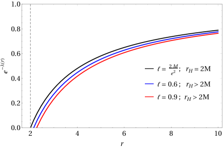
Figure 1: Metric function for different values of $\ell$ with $\alpha=0.4$ and $M=1$. The shift of the horizon $r_{\rm H}$ is controlled by the parameter $\ell$. The Schwarzschild horizon corresponds to the saturated case of the inequality (73).

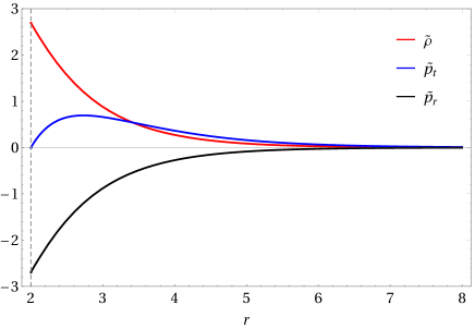
Figure 2: Effective source terms $\times\,10^{4}$ for $\alpha=0.2$. The horizon is located at $r_{\rm H}\gtrsim\,2\,M$, with $M=1$.

The equation determining the horizon $r=r_{\rm H}$ of the metric (68) is given by

$$\alpha\,\ell=r_{\rm H}-2\,M+\alpha\,r_{\rm H}\,e^{-r_{\rm H}/M}\ ,$$ (71)

which allows to write the metric (68) in terms of its horizon in the form

$$e^{\nu}=e^{-\lambda}=1-\frac{\,r_{\rm H}}{r}+\alpha\,\left(e^{-r/M}-\frac{\,r_{\rm H}}{r}\,e^{-r_{\rm H}/M}\right)\ .\quad$$ (72)

It is of course impossible to find analytical solutions to Eq. (71), except for particular values of the parameters. For example, according to our prescription for the SEC, we need $r_{\rm H}\geq 2\,M$, or

$$\ell\geq 2\,M/e^{2}\ .$$ (73)

The extremal case $\ell=2\,M/e^{2}$ leads to the solution

$$e^{\nu}=e^{-\lambda}=1-\frac{2\,M}{r}+\alpha\,\left(e^{-r/M}-\frac{2\,M}{e^{2}\,r}\right)\ .$$ (74)

which has the horizon at $r_{\rm H}=2\,{M}$. The SEC (48) and (49) are both satisfied in the outer region, but the black hole should have the same thermodynamic properties of the Schwarzschild geometry.

The metric function (68) is plotted in Fig. 1 for a given value of $\alpha$, which shows that the horizon is shifted to larger radii when $\ell$ increases from the minimum allowed value (73) corresponding to $r_{\rm H}=2\,{M}$. We find the same behavior when $\alpha$ increases. In this respect, we notice that the effective density ${\tilde{\rho}}$ and pressures ${\tilde{p}}_{r}$ and ${\tilde{p}}_{t}$ in Eqs. (69) and (70) do not depend on the parameter $\ell$, unlike the horizon. This allows us to choose suitable values for the parameters $\alpha$ and $\ell$ such that the SEC is satisfied for $r\gtrsim r_{\rm H}$, as is shown in Fig. 2, where both the density and tangential pressure are positive. We conclude that the metric (68) represents a hairy black hole (having in general non-trivial thermodynamic properties) endowed with the parameters $\{M,\alpha,\ell\}$, where $\ell_{0}=\alpha\,\ell$ represents a charge associated with primary hair.

III.2 Dominant energy condition

We shall next consider the DEC, which requires Visser (1995)

$$\tilde{\rho} \geq |\tilde{p}_{r}|$$ (75)

$$\tilde{\rho} \geq |\tilde{p}_{t}|\ .$$ (76)

In particular, we will see that these conditions allow for deforming the Schwarzschild solution into the Reissner-Nordström-de Sitter geometry with an effective charge $Q$ and an effective cosmological constant $\Lambda$.

We first point out that the inequality (75) is saturated as a consequence of Eq. (32) for a positive effective density, for which Eq. (76) reduces to

$$-\tilde{\rho}\leq\tilde{p}_{t}\leq\tilde{\rho}\ .$$ (77)

We can again write the condition (77) in terms of the definitions (8) and (10) as

$$\theta_{0}^{\ 0}+\,\theta_{2}^{\ 2}\geq 0$$ (78)

$$\theta_{0}^{\ 0}-\,\theta_{2}^{\ 2}\geq 0\ ,$$ (79)

which yield respectively the differential inequalities

$$H_{1}(r)\equiv-r(r-2\,M)h^{\prime\prime}-4(r-M)h^{\prime}-2h+2\geq 0\qquad$$ (80)

$$H_{2}(r)\equiv r\,(r-2\,M)\,h^{\prime\prime}+4\,M\,h^{\prime}-2\,h+2\geq 0\ ,$$ (81)

where we used Eqs. (19) and (21), and $h$ is the same defined in Eq. (37).

We can then notice that $H_{1}(r)=0$ is the differential equation (III) for $a=0$ and $b=-1$. Hence, the bounding solution $h_{1}$ for the extremal case $H_{1}(r)=0$ (with $\alpha\neq\,0$) leads to the line element (39) with $n=2$, namely, the Reissner-Nordström solution (with an effective charge $Q\sim\ell$). On the other hand, $H_{2}(r)=0$ is the differential equation (III) for $a=0$ and $b=1$. Hence, the bounding solution $h_{2}$ for the extremal case $H_{2}(r)=0$ leads to the line element in (39) with $n=-2$, namely, the Schwarzschild-de Sitter solution with cosmological constant $\Lambda\sim\ell^{-2}$. Since $H_{1}(r)=H_{2}(r)=0$ corresponds to vanishing $\theta_{\mu\nu}$ like for the SEC, the unique bounding deformation $h_{0}(r)=h_{1}(r)=h_{2}(r)$ is obtained for $Q=\Lambda=0$, so that the only possible deformation remains again the trivial one in Eq. (61), which yields the seed Schwarzschild solution. Indeed, the functions $H_{1}(r)$ and $H_{2}(r)$ in Eqs. (80) and (81) are also invariant under the transformation (62).

Like in Section III.1, we proceed to investigate deformations which do not saturate the inequalities (80) and (81) everywhere by considering positive functions $H_{1}(r)$ or $H_{2}(r)$ which saturate that inequalities only near the boundaries of the outer region, that is

$$H_{1}(r)=0\qquad{\rm for}\quad\left\{\begin{array}[]{ll}r\sim 2\,M\\ \\ r\gg M\ .\end{array}\right.$$ (82)

In fact, we can still employ the function in Eq. (65) and set

$$H_{1}=M\,G_{\alpha,M}\ .$$ (83)

Upon solving (80) for the corresponding $h$, we obtain

$$h(r)=1-\frac{1}{r-2\,M}\left(\alpha\,\ell+\alpha\,M\,e^{-r/M}-\frac{Q^{2}}{r}\right)\ ,$$ (84)

where $\alpha\,\ell=\ell_{0}$ and $Q$ is also a constant with dimension of a length and proportional to $\alpha$. A second constant of integration was adjusted to meet the proper Schwarzschild limit for $\alpha\to 0$ (in which we remark that $Q\sim\alpha$ vanishes as well). The deformation in Eq. (84) also has to satisfy the inequality (81), which reads

$$\frac{4\,Q^{2}}{r^{2}}\geq\frac{\alpha}{M}\,(r+2\,M)\,e^{-r/M}\ .$$ (85)

Using (84) in the line element (34), we obtain the metric functions

$$e^{\nu}=e^{-\lambda}=1-\frac{2\,M+\alpha\,\ell}{r}+\frac{Q^{2}}{r^{2}}-\frac{\alpha\,M\,e^{-r/M}}{r}\ ,$$ (86)

which is a sort of “charged” version of the solution (68) again with asymptotic mass ${\cal M}=M+\alpha\,\ell/2$. The effective density is now given by

$$\tilde{\rho}=\theta_{0}^{\ 0}=-\tilde{p}_{r}=\frac{Q^{2}}{k^{2}\,r^{4}}-\frac{\alpha\,e^{-r/M}}{k^{2}\,r^{2}}$$ (87)

and an effective tangential pressure reads

$$\tilde{p}_{t}=-\theta_{2}^{\ 2}=\frac{Q^{2}}{k^{2}\,r^{4}}-\frac{\alpha\,e^{-r/M}}{2\,k^{2}\,M\,r}\ .$$ (88)

We can see that

$$\tilde{\rho}-\tilde{p}_{t}=\frac{\alpha\,e^{-r/M}}{2\,k^{2}\,M\,r^{2}}(r-2\,M)$$ (89)

and the DEC is satisfied for $r\geq\,2\,M$, as we originally required. We can also see that the physical singularity at $r=0$ remains.

The horizon radii $r_{\rm H}$ are given by solutions of

$$\alpha\,\ell=r_{\rm H}-2\,M+\frac{Q^{2}}{r_{\rm H}}-\alpha\,M\,e^{-r_{\rm H}/M}\ ,$$ (90)

which allows us to write the metric functions (86) as

$$e^{\nu}=e^{-\lambda} = 1-\frac{r_{\rm H}}{r}\left(1+\frac{Q^{2}}{r_{\rm H}^{2}}-\frac{\alpha\,M}{r_{\rm H}}\,e^{-r_{\rm H}/M}\right)$$ (91)

$$+\frac{Q^{2}}{r^{2}}-\frac{\alpha\,M}{r}\,e^{-r/M}\ .$$

As with the SEC, it is always possible to choose suitable values for the parameters $\alpha$, $\ell$ and $Q$ such that analytical solutions for $r_{\rm H}$ can be found. However, since the DEC requires $r_{\rm H}\geq 2\,M$, the choice of these values cannot be arbitrary. We can see this by evaluating the density (87) at the horizon, in addition to using the expression (90), which yields

$$Q^{2}\geq 4\,\alpha\,(M/e)^{2}\quad{\rm and}\quad\ell\geq M/e^{2}\ .$$ (92)

We remark that $Q$ does not need to be an electric charge. It could be, for instance, a tidal charge of extra-dimensional origin or any other source. However, when $Q$ represents an electric charge, we can say that the electro-vacuum of the Reissner-Nordström geometry also contains a tensor-vacuum whose components are those explicitly proportional to $\alpha$ in Eqs. (87) and (88). Let us recall that the Reissner-Nordström metric has two horizons: the event horizon

$$r_{\rm H}=M+\sqrt{M^{2}-Q^{2}}<2\,M\ ,$$ (93)

and an internal Cauchy horizon given by

$$r_{\rm CH}\equiv M-\sqrt{M^{2}-Q^{2}}<r_{\rm H}\ .$$ (94)

For our solution (86), we can identify at least three cases for which the event horizon $r_{\rm H}$ has simple analytical expressions, and the DEC (75) and (76) are satisfied. As in the Reissner-Nordström metric, each one of these cases has an internal Cauchy horizon $r_{\rm CH}<r_{\rm H}$.

Case 1

Let us start by considering the case saturating the inequalities (92), for which the metric components (91) become

$$e^{\nu}=e^{-\lambda}=1-\frac{2\,M}{r}\left(1+\frac{\alpha}{2\,e^{2}}\right)+\frac{4\,\alpha\,M^{2}}{e^{2}\,r^{2}}-\frac{\alpha\,M}{r}e^{-r/M}\ .$$ (95)

The event horizon is again precisely at $r_{\rm H}=2\,M$, which parallels the case of Eq. (74), and we can also write

$$r_{\rm H}=\frac{e}{\sqrt{\alpha}}\,Q\ .$$ (96)

Notice that by defining

$${\cal M}=M\left(1+\frac{\alpha}{2\,e^{2}}\right)\ ,$$ (97)

the metric functions (95) can be written in a more suggestive form as

$$e^{\nu}=e^{-\lambda}=1-\frac{2\,{\cal M}}{r}+\frac{Q^{2}}{r^{2}}-\frac{\sqrt{\alpha}\,Q}{2\,r}\,e^{1-2\sqrt{\alpha}\,r/e\,Q}\ ,$$ (98)

which can be interpreted as a nonlinear electrodynamics coupled with gravity.

Case 2

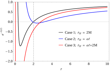
Figure 3: Metric function for the three different analytic cases with $\alpha=0.8$ and $M=1$ for $\ell=0.4$, $4$, $1$, respectively.

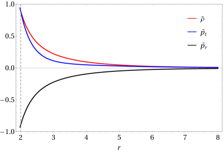
Figure 4: Effective source terms $\times 10^{4}$ for $\alpha=0.1$, $\ell=0.4$, $Q=0.3$, with $M=1$.

The second case we consider is given by

$$Q^{2}=\alpha\,\ell\,M\left(2+\alpha\,e^{-{\alpha\,\ell}/{M}}\right)\ ,$$ (99)

with $\ell\neq 0$, leading to

$$e^{\nu}=e^{-\lambda} = 1-\frac{2\,M+\alpha\,\ell}{r}+\frac{2\,\alpha\,\ell\,M}{r^{2}}$$ (100)

$$-\frac{\alpha\,M}{r^{2}}\,e^{-r/M}\left(r-\alpha\,\ell\,e^{\frac{r-\alpha\,\ell}{M}}\right)\ .$$

The event horizon is now at $r_{\rm H}=\alpha\,\ell=\ell_{0}\geq 2\,M$. If we further assume $\alpha\,\ell\sim\,M$, we can express $M=M(Q)$ from (99) and the metric functions (100) can again be interpreted as a nonlinear electrodynamics coupled with gravity.

Case 3

Finally, we consider

$$Q^{2}=\alpha\,M\left(2\,M+\alpha\,\ell\right)e^{-\frac{(2\,M+\alpha\,\ell)}{M}}\ ,$$ (101)

so that

$$e^{\nu}=e^{-\lambda} = 1-\frac{2\,M+\alpha\,\ell}{r}-\frac{\alpha\,M}{r^{2}}\,e^{-r/M}$$ (102)

$$\times\left[r-\left(2\,M+\alpha\,\ell\right)e^{\frac{r-\left(2\,M+\alpha\,\ell\right)}{M}}\right]\ .$$

The event horizon is at $r_{\rm H}=2\,M+\alpha\,\ell=2\,{\cal M}\geq 2\,M$, and the Schwarzschild horizon is recovered as usual for $\alpha=0$. As in the two previous cases, the interpretation in terms of nonlinear electrodynamics is obtained for $\alpha\,\ell\sim M$.

The metric functions for the three analytical cases in Eqs. (95), (100) and (102) are displayed in Fig. 3, each for a different value of the parameter $\ell$. In all cases the density and pressures have the same qualitative behavior as in Fig. 4, which corresponds to the general case given by Eqs. (86)-(88). We conclude that the metric (86) represents a hairy black hole endowed with the parameters $M$, $Q$, $\alpha$ and $\ell$, where $\{Q,\ell_{0}=\alpha\,\ell\}$ represents a potential set of charges generating primary hair. Among this new family of solutions, we can identify three different cases representing hairy black holes having simple analytical horizons. All these cases can be interpreted as a nonlinear electrodynamics coupled with gravity, whose charges are $M$, $\ell_{0}=\alpha\,\ell$ and $Q$. 

Finally, we want to end by emphasizing a rather important result. When the horizon in (91) has the simple form $r_{\rm H}=K\,M$, with $K\geq 2$ in order to satisfy the DEC, the metric functions become

$$e^{\nu}=e^{-\lambda}=1-\frac{2\,{\cal M}}{r}+\frac{Q^{2}}{r^{2}}-\frac{\alpha\,r_{\rm H}}{K\,r}e^{-K\,r/r_{\rm H}}\ ,$$ (103)

and the event horizon takes the simple Reissner-Nordström form

$$r_{\rm H}=\bar{\cal M}+\sqrt{\bar{\cal M}^{2}-\bar{Q}^{2}}\ ,$$ (104)

where $\bar{\cal M}={\cal M}/\beta$ and $\bar{Q}^{2}={Q}^{2}/\beta$ with

$$\beta=1-\alpha\,\frac{e^{-K}}{K}\ .$$ (105)

We conclude that the metric (103) represents a black hole associated with some non-linear electrodynamics, whose horizon is related with the Reissner-Nordström one by the quite simple expression

$$r_{\rm H}=\frac{r_{\rm RN}}{\beta}\geq r_{\rm RN}\ ,$$ (106)

since $\beta\leq 1$. In order to specify this nonlinear electrodynamics, we identify

$$\theta_{\mu\nu}=-\left[L_{F}\,F_{\mu\alpha}\,F^{\alpha}{}_{\nu}+L(F)\,g_{\mu\nu}\right]\ ,$$ (107)

where

$$F=\frac{1}{4}\,F_{\mu\nu}\,F^{\mu\nu}\quad{\rm and}\quad L_{F}=\frac{dL}{dF}\ .$$ (108)

In the static spherically symmetric case, we have

$$F_{\mu\nu}=E(r)\,\left(\delta^{0}_{\mu}\,\delta^{1}_{\nu}-\delta^{1}_{\mu}\,\delta^{0}_{\nu}\right)\ .$$ (109)

Following a standard procedure, we then obtain the electric field

$$E(r)=\frac{Q}{r^{2}}-\frac{\alpha\,e^{-\frac{K\,r}{r_{\rm H}}}(K\,r+2\,r_{\rm H})}{4\,r_{\rm H}\,Q}\ .$$ (110)

We can describe the underlying nonlinear electrodynamics within the $P$-dual formalism Salazar et al. (1987); Ayon-Beato and Garcia (1998), which yields the Lagrangian

$$L(P)=-4\,\pi\,P-\frac{\alpha\,K\,\sqrt[4]{-2\,P}\,e^{\mathcal{G}(P)}}{4\,\sqrt{\pi}\,\sqrt{Q}\,r_{\rm H}}\ ,$$ (111)

with

$$\mathcal{G}(P)=-\frac{K\,\sqrt{Q}}{2\,\sqrt{\pi}\,\sqrt[4]{-2\,P}\,r_{\rm H}}\ ,$$ (112)

where

$$P=\frac{1}{4}\,P_{\mu\nu}\,P^{\mu\nu}\quad{\rm and}\quad P_{\mu\nu}=L_{F}\,F_{\mu\nu}\ .$$ (113)

We want to conclude emphasizing once again that $Q^{2}\sim\alpha$, so that the Schwarzschild geometry is always recovered for $\alpha\to 0$. However, when $Q$ represents an electric charge, we can say that the electro-vacuum (Reissner-Nordström geometry) is filled with a tensor-vacuum whose origin lies in the nonlinear electrodynamics with the Lagrangian (111).

IV Conclusions

Using the EGD approach, we studied the emergence of hairy black holes due to matter surrounding the central source of the Schwarzschild metric. Demanding that the solution always admits a well defined horizon through Eq. (30), and that the hair satisfies the SEC or DEC through Eqs. (47) or (75) and (76), respectively, we found two new families of hairy black holes displayed in Eqs. (68) and (86). These geometries were analysed and, in particular, we found that the solutions satisfying the DEC contain the non-trivial extension of the Reissner-Nordström black hole shown in (103) which possesses a simple event horizon. The Lagrangian of the nonlinear electrodynamics, which sources this solution, was also obtained explicitly.

From the technical point of view, since aim of the present work was to study some general conditions under which hair can be added to the (spherically symmetric) vacuum black holes of general relativity, the EGD was the natural approach to employ from the onset. In fact, the EGD is precisely devised for describing deformations of known solutions of general relativity induced by adding extra sources. Moreover, the properties of the added source were restricted in order to enforce the conditions mentioned above, rather than assuming the hair is described in terms of fundamental fields. Nonetheless, we were able to give a description in terms of a nonlinear electrodynamics at least in one specific case.

Finally, we would like to remark that the charges $Q$ and $\ell_{0}=\alpha\,\ell$ associated with our hairy black holes admit simple physical interpretations. The charge $Q$ can be viewed as an effective electric charge and is proportional to $\alpha$, which is the generic parameter measuring the deviation from the chosen vacuum solution (which is given by the Schwarzschild metric). A special mention deserves the parameter $\ell_{0}$, which is associated with gauge transformations of the seed Schwarzschild metric and which seems to always push the event horizon to radii larger than the Schwarzschild radius. Therefore $\ell_{0}=\alpha\,\ell$ measures how much the entropy of the black hole increases from its minimum Schwarzschild value $S=4\,\pi\,{M^{2}}$ when hair is added.

Acknowledgments

R.C. is partially supported by the INFN grant FLAG and his work has also been carried out in the framework of activities of the National Group of Mathematical Physics (GNFM, INdAM) and COST action Cantata.

References

- Abbott et al. (2016) B. P. Abbott et al. (LIGO Scientific, Virgo), Phys. Rev. Lett. 116, 061102 (2016), arXiv:1602.03837 [gr-qc] .
- Abbott et al. (2017) B. P. Abbott et al. (LIGO Scientific, Virgo), Phys. Rev. Lett. 119, 141101 (2017), arXiv:1709.09660 [gr-qc] .
- Akiyama et al. (2019) K. Akiyama et al. (Event Horizon Telescope), Astrophys. J. 875, L1 (2019).
- Ruffini and Wheeler (1971) R. Ruffini and J. A. Wheeler, Phys. Today 24, 30 (1971).
- Hawking (1972) S. Hawking, Commun. Math. Phys. 25, 152 (1972).
- Hawking et al. (2016) S. W. Hawking, M. J. Perry, and A. Strominger, Phys. Rev. Lett. 116, 231301 (2016), arXiv:1601.00921 [hep-th] .
- Sotiriou and Faraoni (2012) T. P. Sotiriou and V. Faraoni, Phys. Rev. Lett. 108, 081103 (2012), arXiv:1109.6324 [gr-qc] .
- Babichev and Charmousis (2014) E. Babichev and C. Charmousis, JHEP 08, 106 (2014), arXiv:1312.3204 [gr-qc] .
- Cisterna and Erices (2014) A. Cisterna and C. Erices, Phys. Rev. D 89, 084038 (2014), arXiv:1401.4479 [gr-qc] .
- Sotiriou and Zhou (2014) T. P. Sotiriou and S.-Y. Zhou, Phys. Rev. Lett. 112, 251102 (2014), arXiv:1312.3622 [gr-qc] .
- Antoniou et al. (2018a) G. Antoniou, A. Bakopoulos, and P. Kanti, Phys. Rev. Lett. 120, 131102 (2018a), arXiv:1711.03390 [hep-th] .
- Antoniou et al. (2018b) G. Antoniou, A. Bakopoulos, and P. Kanti, Phys. Rev. D 97, 084037 (2018b), arXiv:1711.07431 [hep-th] .
- Grumiller et al. (2020) D. Grumiller, A. Pérez, M. Sheikh-Jabbari, R. Troncoso, and C. Zwikel, Phys. Rev. Lett. 124, 041601 (2020), arXiv:1908.09833 [hep-th] .
- Volkov and Galtsov (1989) M. Volkov and D. Galtsov, JETP Lett. 50, 346 (1989).
- Kanti et al. (1996) P. Kanti, N. Mavromatos, J. Rizos, K. Tamvakis, and E. Winstanley, Phys. Rev. D 54, 5049 (1996), arXiv:hep-th/9511071 .
- Kanti et al. (1998) P. Kanti, N. Mavromatos, J. Rizos, K. Tamvakis, and E. Winstanley, Phys. Rev. D 57, 6255 (1998), arXiv:hep-th/9703192 .
- Zloshchastiev (2005) K. G. Zloshchastiev, Phys. Rev. Lett. 94, 121101 (2005), arXiv:hep-th/0408163 .
- Martinez et al. (2004) C. Martinez, R. Troncoso, and J. Zanelli, Phys. Rev. D 70, 084035 (2004), arXiv:hep-th/0406111 .
- Herdeiro and Radu (2015) C. A. Herdeiro and E. Radu, Int. J. Mod. Phys. D 24, 1542014 (2015), arXiv:1504.08209 [gr-qc] .
- Sotiriou (2015) T. P. Sotiriou, Class. Quant. Grav. 32, 214002 (2015), arXiv:1505.00248 [gr-qc] .
- Ovalle et al. (2018a) J. Ovalle, R. Casadio, R. d. Rocha, A. Sotomayor, and Z. Stuchlik, Eur. Phys. J. C78, 960 (2018a), arXiv:1804.03468 [gr-qc] .
- Ovalle (2019) J. Ovalle, Phys. Lett. B788, 213 (2019), arXiv:1812.03000 [gr-qc] .
- Ovalle (2017) J. Ovalle, Phys. Rev. D95, 104019 (2017), arXiv:1704.05899 [gr-qc] .
- Ovalle (2008) J. Ovalle, Mod. Phys. Lett. A23, 3247 (2008), arXiv:gr-qc/0703095 [gr-qc] .
- Ovalle and Casadio (2020) J. Ovalle and R. Casadio, Beyond Einstein Gravity, SpringerBriefs in Physics (Springer Nature, Cham, 2020).
- Ovalle (2009) J. Ovalle, Int. J. Mod. Phys. D 18, 837 (2009), arXiv:0809.3547 [gr-qc] .
- Ovalle (2010) J. Ovalle, Mod. Phys. Lett. A 25, 3323 (2010), arXiv:1009.3674 [gr-qc] .
- Casadio and Ovalle (2012) R. Casadio and J. Ovalle, Phys. Lett. B715, 251 (2012), arXiv:1201.6145 [gr-qc] .
- Casadio and Ovalle (2014) R. Casadio and J. Ovalle, Gen. Rel. Grav. 46, 1669 (2014), arXiv:1212.0409 [gr-qc] .
- Ovalle et al. (2013) J. Ovalle, F. Linares, A. Pasqua, and A. Sotomayor, Class. Quant. Grav. 30, 175019 (2013), arXiv:1304.5995 [gr-qc] .
- Casadio et al. (2014) R. Casadio, J. Ovalle, and R. da Rocha, Class. Quant. Grav. 31, 045016 (2014), arXiv:1310.5853 [gr-qc] .
- Ovalle and Linares (2013) J. Ovalle and F. Linares, Phys. Rev. D88, 104026 (2013), arXiv:1311.1844 [gr-qc] .
- Ovalle et al. (2015) J. Ovalle, L. A. Gergely, and R. Casadio, Class. Quant. Grav. 32, 045015 (2015), arXiv:1405.0252 [gr-qc] .
- Casadio et al. (2015a) R. Casadio, J. Ovalle, and R. da Rocha, EPL 110, 40003 (2015a), arXiv:1503.02316 [gr-qc] .
- Casadio et al. (2015b) R. Casadio, J. Ovalle, and R. da Rocha, Class. Quant. Grav. 32, 215020 (2015b), arXiv:1503.02873 [gr-qc] .
- Ovalle (2015) J. Ovalle, Proceedings, 9th Alexander Friedmann International Seminar on Gravitation and Cosmology and 3rd Satellite Symposium on the Casimir Effect: St. Petersburg, Russia, June 21-27, 2015, (2015), 10.1142/S2010194516601320, [Int. J. Mod. Phys. Conf. Ser.41,1660132(2016)], arXiv:1510.00855 [gr-qc] .
- Cavalcanti et al. (2016) R. T. Cavalcanti, A. G. da Silva, and R. da Rocha, Class. Quant. Grav. 33, 215007 (2016), arXiv:1605.01271 [gr-qc] .
- da Rocha (2017a) R. da Rocha, Phys. Rev. D95, 124017 (2017a), arXiv:1701.00761 [hep-ph] .
- da Rocha (2017b) R. da Rocha, Eur. Phys. J. C77, 355 (2017b), arXiv:1703.01528 [hep-th] .
- Fernandes-Silva and da Rocha (2018) A. Fernandes-Silva and R. da Rocha, Eur. Phys. J. C78, 271 (2018), arXiv:1708.08686 [hep-th] .
- Casadio et al. (2018) R. Casadio, P. Nicolini, and R. da Rocha, Class. Quant. Grav. 35, 185001 (2018), arXiv:1709.09704 [hep-th] .
- Fernandes-Silva et al. (2018) A. Fernandes-Silva, A. J. Ferreira-Martins, and R. Da Rocha, Eur. Phys. J. C78, 631 (2018), arXiv:1803.03336 [hep-th] .
- Contreras and Bargueño (2018) E. Contreras and P. Bargueño, Eur. Phys. J. C78, 558 (2018), arXiv:1805.10565 [gr-qc] .
- Contreras (2018) E. Contreras, Eur. Phys. J. C78, 678 (2018), arXiv:1807.03252 [gr-qc] .
- Contreras and Bargueño (2018) E. Contreras and P. Bargueño, Eur. Phys. J. C 78, 985 (2018), arXiv:1809.09820 [gr-qc] .
- Panotopoulos and Rincón (2018) G. Panotopoulos and A. Rincón, Eur. Phys. J. C78, 851 (2018), arXiv:1810.08830 [gr-qc] .
- Da Rocha and Tomaz (2019) R. Da Rocha and A. A. Tomaz, Eur. Phys. J. C 79, 1035 (2019), arXiv:1905.01548 [hep-th] .
- Las Heras and León (2019) C. Las Heras and P. León, Eur. Phys. J. C 79, 990 (2019), arXiv:1905.02380 [gr-qc] .
- Rincón et al. (2019) A. Rincón, L. Gabbanelli, E. Contreras, and F. Tello-Ortiz, Eur. Phys. J. C 79, 873 (2019), arXiv:1909.00500 [gr-qc] .
- da Rocha (2020a) R. da Rocha, Symmetry 12, 508 (2020a), arXiv:2002.10972 [hep-th] .
- Contreras et al. (2020) E. Contreras, F. Tello-Ortíz, and S. Maurya, (2020), arXiv:2002.12444 [gr-qc] .
- Arias et al. (2020) C. Arias, F. Tello Ortiz, and E. Contreras, Eur. Phys. J. C 80, 463 (2020), arXiv:2003.00256 [gr-qc] .
- da Rocha (2020b) R. da Rocha, (2020b), arXiv:2003.12852 [hep-th] .
- Tello-Ortiz et al. (2020) F. Tello-Ortiz, S. Maurya, and Y. Gomez-Leyton, Eur. Phys. J. C 80, 324 (2020).
- da Rocha and Tomaz (2020) R. da Rocha and A. A. Tomaz, (2020), arXiv:2005.02980 [hep-th] .
- Meert and da Rocha (2020) P. Meert and R. da Rocha, (2020), arXiv:2006.02564 [gr-qc] .
- Ovalle et al. (2018b) J. Ovalle, R. Casadio, R. da Rocha, and A. Sotomayor, Eur. Phys. J. C78, 122 (2018b), arXiv:1708.00407 [gr-qc] .
- Gabbanelli et al. (2018) L. Gabbanelli, A. Rincón, and C. Rubio, Eur. Phys. J. C78, 370 (2018), arXiv:1802.08000 [gr-qc] .
- Heras and Leon (2018) C. L. Heras and P. Leon, Fortsch. Phys. 66, 1800036 (2018), arXiv:1804.06874 [gr-qc] .
- Estrada and Tello-Ortiz (2018) M. Estrada and F. Tello-Ortiz, Eur. Phys. J. Plus 133, 453 (2018), arXiv:1803.02344 [gr-qc] .
- Sharif and Sadiq (2018a) M. Sharif and S. Sadiq, Eur. Phys. J. C78, 410 (2018a), arXiv:1804.09616 [gr-qc] .
- Morales and Tello-Ortiz (2018a) E. Morales and F. Tello-Ortiz, Eur. Phys. J. C78, 618 (2018a), arXiv:1805.00592 [gr-qc] .
- Sharif and Sadiq (2018b) M. Sharif and S. Sadiq, Eur. Phys. J. Plus 133, 245 (2018b).
- Morales and Tello-Ortiz (2018b) E. Morales and F. Tello-Ortiz, Eur. Phys. J. C78, 841 (2018b), arXiv:1808.01699 [gr-qc] .
- Estrada and Prado (2019) M. Estrada and R. Prado, Eur. Phys. J. Plus 134, 168 (2019), arXiv:1809.03591 [gr-qc] .
- Sharif and Saba (2018) M. Sharif and S. Saba, Eur. Phys. J. C78, 921 (2018), arXiv:1811.08112 [gr-qc] .
- Ovalle et al. (2018c) J. Ovalle, R. Casadio, R. da Rocha, A. Sotomayor, and Z. Stuchlik, EPL 124, 20004 (2018c), arXiv:1811.08559 [gr-qc] .
- Contreras (2019) E. Contreras, Class. Quant. Grav. 36, 095004 (2019), arXiv:1901.00231 [gr-qc] .
- Maurya and Tello-Ortiz (2019) S. K. Maurya and F. Tello-Ortiz, Eur. Phys. J. C79, 85 (2019).
- Contreras et al. (2019) E. Contreras, A. Rincón, and P. Bargueño, Eur. Phys. J. C79, 216 (2019), arXiv:1902.02033 [gr-qc] .
- Contreras and Bargueño (2019) E. Contreras and P. Bargueño, Class. Quant. Grav. 36, 215009 (2019), arXiv:1902.09495 [gr-qc] .
- Gabbanelli et al. (2019) L. Gabbanelli, J. Ovalle, A. Sotomayor, Z. Stuchlik, and R. Casadio, Eur. Phys. J. C 79, 486 (2019), arXiv:1905.10162 [gr-qc] .
- Estrada (2019) M. Estrada, Eur. Phys. J. C 79, 918 (2019), arXiv:1905.12129 [gr-qc] .
- Ovalle et al. (2019) J. Ovalle, C. Posada, and Z. Stuchlík, Class. Quant. Grav. 36, 205010 (2019), arXiv:1905.12452 [gr-qc] .
- Maurya and Tello-Ortiz (2020) S. Maurya and F. Tello-Ortiz, Phys. Dark Univ. 27, 100442 (2020), arXiv:1905.13519 [gr-qc] .
- Hensh and Stuchlík (2019) S. Hensh and Z. e. Stuchlík, Eur. Phys. J. C 79, 834 (2019), arXiv:1906.08368 [gr-qc] .
- Linares Cedeño and Contreras (2020) F. X. Linares Cedeño and E. Contreras, Phys. Dark Univ. 28, 100543 (2020), arXiv:1907.04892 [gr-qc] .
- León and Sotomayor (2019) P. León and A. Sotomayor, Fortsch. Phys. 67, 1900077 (2019), arXiv:1907.11763 [gr-qc] .
- Torres-Sánchez and Contreras (2019) V. Torres-Sánchez and E. Contreras, Eur. Phys. J. C 79, 829 (2019), arXiv:1908.08194 [gr-qc] .
- Casadio et al. (2019) R. Casadio, E. Contreras, J. Ovalle, A. Sotomayor, and Z. Stuchlick, Eur. Phys. J. C 79, 826 (2019), arXiv:1909.01902 [gr-qc] .
- Singh et al. (2019) K. Singh, S. Maurya, M. Jasim, and F. Rahaman, Eur. Phys. J. C 79, 851 (2019).
- Maurya (2019) S. Maurya, Eur. Phys. J. C 79, 958 (2019).
- Sharif and Waseem (2019) M. Sharif and A. Waseem, Annals Phys. 405, 14 (2019).
- Abellán et al. (2020) G. Abellán, V. Torres-Sánchez, E. Fuenmayor, and E. Contreras, Eur. Phys. J. C 80, 177 (2020), arXiv:2001.08573 [gr-qc] .
- Sharif and Ama-Tul-Mughani (2020) M. Sharif and Q. Ama-Tul-Mughani, Annals Phys. 415, 168122 (2020), arXiv:2004.07925 [gr-qc] .
- Tello-Ortiz (2020) F. Tello-Ortiz, Eur. Phys. J. C 80, 413 (2020).
- Maurya (2020) S. Maurya, Eur. Phys. J. C 80, 429 (2020).
- Rincón et al. (2020) A. Rincón, E. Contreras, F. Tello-Ortiz, P. Bargueño, and G. Abellán, Eur. Phys. J. C 80, 490 (2020), arXiv:2005.10991 [gr-qc] .
- Sharif and Majid (2020) M. Sharif and A. Majid, Phys. Dark Univ. 30, 100610 (2020), arXiv:2006.04578 [gr-qc] .
- Maurya et al. (2020) S. Maurya, K. N. Singh, and B. Dayanandan, Eur. Phys. J. C 80, 448 (2020).
- Herrera and Santos (1997) L. Herrera and N. O. Santos, Phys. Rept. 286, 53 (1997).
- Mak and Harko (2003) M. K. Mak and T. Harko, Proc. Roy. Soc. Lond. A459, 393 (2003), arXiv:gr-qc/0110103 [gr-qc] .
- Kiselev (2003) V. Kiselev, Class. Quant. Grav. 20, 1187 (2003), arXiv:gr-qc/0210040 .
- Visser (2020) M. Visser, Class. Quant. Grav. 37, 045001 (2020), arXiv:1908.11058 [gr-qc] .
- Visser (1995) M. Visser, Lorentzian wormholes: From Einstein to Hawking (1995).
- Curiel (2017) E. Curiel, “A Primer on Energy Conditions,” (2017) pp. 43–104, arXiv:1405.0403 [physics.hist-ph] .
- Salazar et al. (1987) I. Salazar, A. Garcia, and J. Plebanski, J. Math. Phys. 28, 2171 (1987).
- Ayon-Beato and Garcia (1998) E. Ayon-Beato and A. Garcia, Phys. Rev. Lett. 80, 5056 (1998), arXiv:gr-qc/9911046 .