Bandits with Partially Observable Confounded Data

Abstract

We study linear contextual bandits with access to a large, confounded, offline dataset that was sampled from some fixed policy. We show that this problem is closely related to a variant of the bandit problem with side information. We construct a linear bandit algorithm that takes advantage of the projected information, and prove regret bounds. Our results demonstrate the ability to take advantage of confounded offline data. Particularly, we prove regret bounds that improve current bounds by a factor related to the visible dimensionality of the contexts in the data. Our results indicate that confounded offline data can significantly improve online learning algorithms. Finally, we demonstrate various characteristics of our approach through synthetic simulations.

1 Introduction

The use of offline data for online control is of practical interest in fields such as autonomous driving, healthcare, dialogue systems, and recommender systems [Mirchevska et al., 2017, Murphy et al., 2001, Li et al., 2016, Covington et al., 2016]. There, an abundant amount of data is readily available, potentially encompassing years of logged experience. This data can greatly reduce the need to interact with the real world, as such interactions may be both costly and unsafe [Amodei et al., 2016]. Nevertheless, as offline data is usually generated in an uncontrolled manner, it poses major challenges, such as unobserved states and actions. Failing to take these into account may result in biased estimates that are confounded by spurious correlation [Gottesman et al., 2019a]. This work focuses on utilizing partially observable offline data in an online bandit setting.

We consider the stochastic linear contextual bandit setting [Auer, 2002, Chu et al., 2011, Zhou et al., 2019]. Here, the context is a vector $x\in\mathbb{R}^{d}$ encompassing the full state of information. We assume to have additional access to an offline dataset in which only $L<d$ covariates (features) of the context are available. The unobserved covariates in the data are known as unobserved confounding factors in the causal inference literature [Pearl and Mackenzie, 2018], which may cause spurious associations in the data, rendering the data useless unless further assumptions are made [Neuberg, 2003, Shpitser and Pearl, 2012, Bareinboim et al., 2015]. In this work we assume that, when interacting with the online environment, the full context is accessible, and search for methods to combine both sources of information (online and offline) to quickly converge to an optimal solution.

We construct an algorithm that is provably superior to an algorithm which does not utilize the (partially observable) information in the data. We recognize the following fundamental observation: Confounded offline data can (still) be used to improve online learning, and specifically, that partially observable offline data can be utilized as linear side information (linear constraints) for the bandit problem.

While the bandit setting with confounded offline data has already been explored, its combination with a fully observable online environment is a new setting with particular challenges and benefits. First, one cannot ensure identification of an optimal policy with confounded offline data (see Section 3). This has implications on safety and applicability of algorithms which are based solely on offline data, e.g., the confounding bias of offline critical care datasets [Johnson et al., 2016]. Second, in contemporary widespread applications, an abundant of offline data is readily available. These application do not necessarily prevent interactions with the real world. On the contrary, countless real-world applications can access the real world. Still, such interactions may be costly, time consuming, or unsafe. It is thus vital to utilize the enormous amounts of previously collected offline data to reduce as much as possible the need for online interactions. We discuss two concrete examples from the healthcare and traffic management domains below.

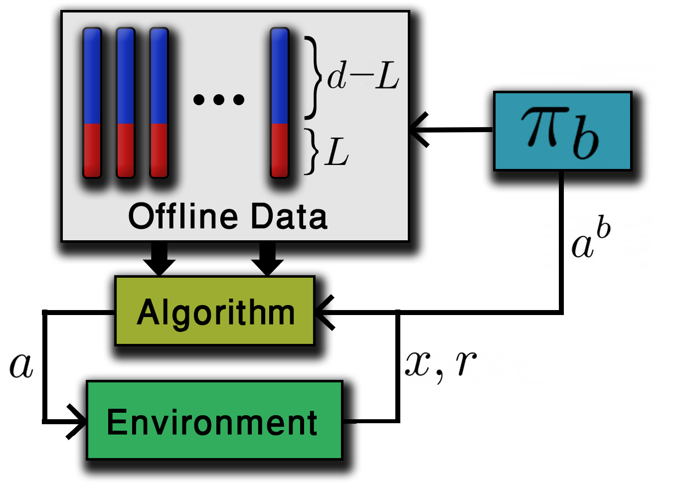
(a) (a)

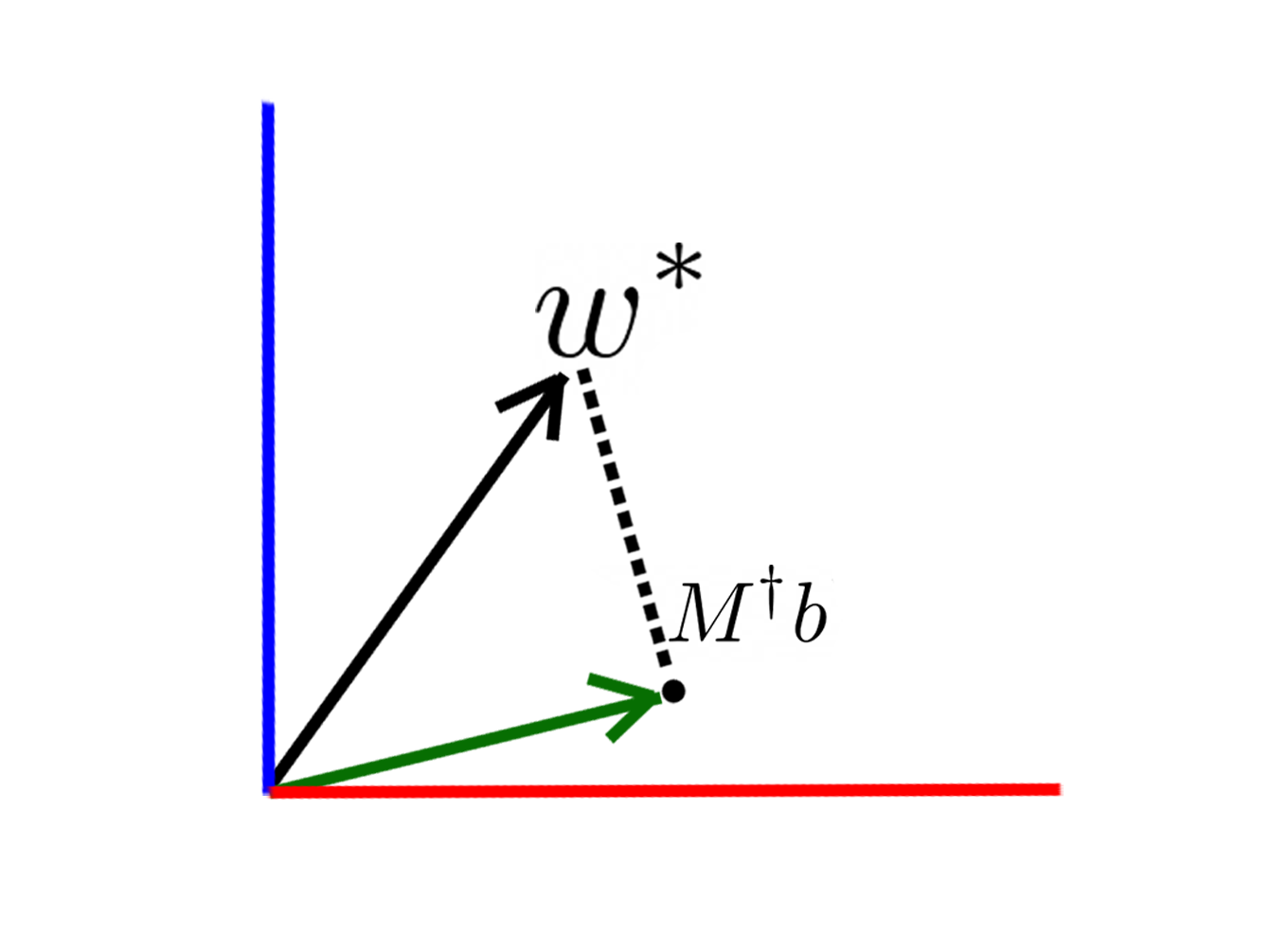
(b) (b)

Figure 1: (a) Block diagram of our setup: an online learner interacting with an environment while utilizing partially observable offline data that was generated by a behavior policy $\pi_{b}$. (b) This plot depicts the projection of $Mw^{*}=b$. We show that partially observable offline data can provide us with approximate linear side information of this form. The online learner must then estimate the orthogonal subspace, attempting to reduce the effective dimensionality of the problem.

Healthcare. Consider the important challenge of cancer chemotherapy control; specifically, optimal drug dosing for cancer chemotherapy [Sbeity and Younes, 2015]. Clinicians usually follow established guidelines for treating each patient, prescribing drug doses according to the stage of the tumor, the weight of the patient, white blood cell levels, concurrent illnesses, and the age of the patient. Suppose we are given access to large amounts of medical records of chemotherapy plans, specifying the frequency and dose of drug administration as well as their effect on the patient. Due to privacy regulations, the patients’ socioeconomic characteristics are removed from the data. Nevertheless, these features may have affected the physician’s decisions, as well as the outcome of the prescribed treatments. Next, suppose we are able to interact with the world, where the full state of the patients’ information is available to us. How would we efficiently construct an algorithm to automate chemotherapy treatment while also utilizing the partially observable, confounded data?

Smart City Traffic Management. Consider the problem of adjusting traffic signals based on real-time traffic conditions using video footage of cameras located over intersections. The development time of the system consists of continual addition of new labels (classes) for the different types of vehicles and pedestrians based on relevant characteristics that may affect traffic congestion. Due to this recurrent process, data that was gathered in previous times may render itself useless, outdated, and even harmless, unless handled properly. This is due to the fact that some of the new information in the state was not previously collected, yet is needed for training future control strategies. How should one use the partially observable historical data for improving the most recent online system?

In this work we show how the confounded information in the data can be utilized for the online bandit problem. Figures 1 and 2 illustrate our basic setup and approach. We show how confounded offline data can be thought of as linear constraints to the online problem. These linear constraints, are not fully known. They are in fact dependent on the cross-correlation matrix of the context vector induced by policy that generated the data (which we denote as the behavior policy, $\pi_{b}$). To learn these constraints and utilize them, we approximate the cross-correlation matrix through online interactions and carefully integrate them into our learning algorithm, decreasing the overall regret.

The contributions of our work are as follows. As a fundamental contribution we propose a framework for combining confounded offline data with online learning. This framework is a gateway between fully confounded offline data to online learning, and encompasses a variety of important problems and applications. While this work only considers the linear bandit setting, it sets the building blocks and insights needed for more complex settings (e.g., reinforcement learning). Our second contribution shows that partially observable confounded data can in fact be realized as linear constraints for the online problem (see Section 3). To the best of our knowledge, this work is the first to show this relation. Finally, we prove that the overall regret can indeed be decreased when using the confounded data. Our proof, too, consists of technical obstacles related to the approximate constraints, which must be learned simultaneously.

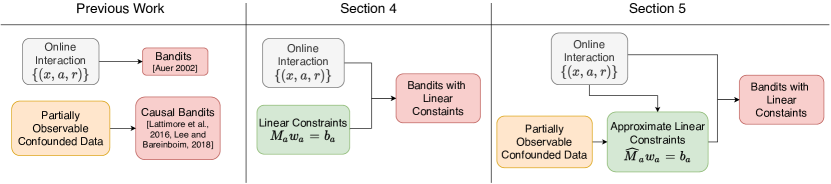
Figure 2: Previous work has dealt with bandits in the online setting. Other work integrated causal information to utilize confounded offline data. This work combines the two through constraints on the online problem. In Section 4 we show how linear constraints can be leveraged to achieve better regret for the bandit problem (Theorem 1). Then, in Section 5 partial linear constraints are estimated from online interactions, and then utilized efficiently by our learning algorithm. Note that $b_{a}$ is not estimated as it is previously computed from the offline data (see Section 3). Finally, due to fast convergence of the linear constraints, improved performance is still achieved (Theorem 2).

2 Problem Setting

Notations. We use $[n]$ to denote the set $\brk[c]*{1,\ldots,n}$. We denote by $I_{m}$ the $m\times m$ identity matrix. Let $y,z\in\mathbb{R}^{d}$ and $A,B\in\mathbb{R}^{d\times d}$. We use $\left\lVert z\right\rVert_{2}$ to denote the $\ell_{2}$-norm and $z^{T}$ the transpose of $z$. The inner product is represented as $\brk[a]*{z,y}$. For $A$ semi-positive definite, the weighted $\ell_{2}$-norm is denoted by $\left\lVert z\right\rVert_{A}=\sqrt{z^{T}Az}$. The minimum and maximum singular values of $A$ are denoted by $\lambda_{min}(A)$ and $\lambda_{max}(A)$ respectively. Furthermore, $A\preceq B$ if $B-A$ is positive semi-definite. The spectral norm of $A$ is denoted by ${\left\lVert A\right\rVert_{2}=\sup_{\left\lVert x\right\rVert_{2}=1}\left\lVert Ax\right\rVert_{2}}$. The Moore-Penrose inverse of $A$ is denoted by $A^{\dagger}$. Finally, we use $\mathcal{O}(x)$ to refer to a quantity that depends on $x$ up to a poly-log expression in $d,T$ and $\delta$, and $\widetilde{\mathcal{O}}(x)$ represents the leading dependence of $x$ in $d,T$ and $K$.

Setup. Our basic framework consists of sequential interactions of a learner with an environment. We assume the following protocol, which proceeds in discrete trials $t=1,\ldots,T$. At each round $t\in[T]$ the environment outputs a context $x_{t}\in\mathcal{X}\subseteq\mathbb{R}^{d}$ sampled from some unknown distribution $\mathcal{P}_{x}$. We assume that $x_{1},\ldots x_{T}$ are i.i.d. Based on observed payoffs in previous trials, the learner chooses an action $a_{t}\in\mathcal{A}$, where $\mathcal{A}=[K]$ is the learner’s action space. Subsequently, the learner observes a reward $r_{t}=\brk[a]*{x_{t},w^{*}_{a_{t}}}+\eta_{t}$, where $\brk[c]*{w^{*}_{a}\in\mathbb{R}^{d}}_{a\in\mathcal{A}}$ are unknown parameter vectors, and $\eta_{t}$ is some conditionally $\sigma$-subgaussian random noise, i.e., for some $\sigma>0$

$$\mathbb{E}^{#1}\left[\nonscript\,e^{\lambda\eta_{t}}\nonscript\;\middle|\nonscript\>\allowbreak F_{t-1}\nonscript\,\right]\leq\exp\left(\frac{\lambda^{2}\sigma^{2}}{2}\right)$$

Here, $\brk[c]*{F_{t}}_{t=0}^{\infty}$ is any filtration of $\sigma$-algebras such that for any $t\geq 1$, $x_{t}$ is $F_{t-1}$-measurable and $\eta_{t}$ is $F_{t}$-measurable, e.g., the natural $\sigma$-algebra $F_{t-1}=\sigma\left((x_{1},a_{1},\eta_{1}),\ldots,(x_{t-1},a_{t-1},\eta_{t-1}),x_{t},a_{t}\right)$.

The goal of the learner is to maximize the total reward $\sum_{t=1}^{T}\brk[a]*{x_{t},w^{*}_{a_{t}}}$ accumulated over the course of $T$ rounds. We evaluate the learner against the optimal strategy, which has knowledge of $\brk[c]*{w^{*}_{a}\in\mathbb{R}^{d}}_{a\in\mathcal{A}}$, namely $\pi^{*}(x)\in\arg\max_{a\in\mathcal{A}}\brk[a]*{x,w^{*}_{a}}$. The difference between the learner and optimal strategy’s total reward is known as the regret, and is given by

$${\textit{Regret}\left(T\right)=\sum_{t=1}^{T}\brk[a]*{x_{t},w^{*}_{\pi^{*}(x_{t})}}-\sum_{t=1}^{T}\brk[a]*{x_{t},w^{*}_{a_{t}}}.}$$

In this work we assume to have additional access to a partially observable offline dataset, consisting of partially observable contexts, actions, and rewards. Specifically, we assume a dataset ${\mathcal{D}=\brk[c]*{Qx_{i},a_{i},r_{i}}_{i=1}^{N}}$, in which $\brk[c]*{x_{i}}_{i=1}^{N}$ are i.i.d. samples from $\mathcal{P}_{x}$, $\brk[c]*{a_{i}}_{i=1}^{N}$ were generated by some fixed behavior policy, denoted by $\pi_{b}$, which is a mapping from contexts $x\in\mathcal{X}$ to a probability over actions, and $\brk[c]*{r_{i}}_{i=1}^{N}$ were generated by the same model described above. Here, we used $Q\in\mathbb{R}^{L\times d}$ to denote the rectangular matrix $Q=\begin{pmatrix}I_{L}&0\end{pmatrix}$. That is, without loss of generality, we assume only the first $L$ features of $x_{i}$ are visible in the data. Throughout our work we will sometimes use the notation $x^{\mathrm{o}}$ and $x^{\mathrm{h}}$ to denote the observed and unobserved (hidden) covariates of $x$, respectively. That is, $x=\begin{pmatrix}(x^{\mathrm{o}})^{T},(x^{\mathrm{h}})^{T}\end{pmatrix}^{T}$, where $x^{\mathrm{o}}\in\mathbb{R}^{L},\ x^{\mathrm{h}}\in\mathbb{R}^{d-L}$.

Notice that the distribution of $\mathcal{D}=\brk[c]*{x^{\mathrm{o}}_{i},a_{i},r_{i}}_{i=1}^{N}$, the partially observable dataset, depends on $\pi_{b}$. Any statistic we attempt to draw from the offline data depends on the measure induced by $\pi_{b}$, which we denote by $P^{\pi_{b}}$ . Figure 1 depicts a diagram of our basic setup and approach.

3 From Partially Observable Offline Data to Linear Side Information

Consider only having access to the partially observable offline data $\mathcal{D}$. Having access to such data is mostly useless without further assumptions. Particularly, $w^{*}_{a}$ may not be identifiable . In fact, it can be shown that for any behavioral policy $\pi_{b}$ and induced measure $P^{\pi_{b}}$, $\brk[c]*{w_{a}^{*}}_{a\in\mathcal{A}}$ are not identifiable. More specifically, for all ${w^{1}=\brk[c]*{w_{a}^{1}}_{a\in\mathcal{A}}}$, exist ${w^{2}=\brk[c]*{w_{a}^{2}}_{a\in\mathcal{A}}\neq w^{2}}$ and probability measures $P_{1},P_{2}$ such that ${P_{1}\left(x^{\mathrm{o}},a,r;w^{1},\pi_{b}\right)=P_{2}\left(x^{\mathrm{o}},a,r;w^{2},\pi_{b}\right)}$ and ${\pi_{b}\left(a,x;w^{1}\right)=\pi_{b}\left(a,x;w^{2}\right)}$. This claim is a standard type of result. A proof is provided in the supplementary material.

To mitigate the identification problem, prior knowledge of characteristics of $\brk[c]*{w_{a}^{*}}_{a\in\mathcal{A}}$ can be leveraged [Cinelli et al., 2019]. Instead, here we consider access to an online environment, where the covariates that were unobserved in the data are supplied, i.e., fully observed. This enables us to deconfound the data and identify $\brk[c]*{w_{a}^{*}}_{a\in\mathcal{A}}$.

Prior to constructing our algorithmic approach, we discuss the relation of confounded offline data to partially known linear constraints. This connection is a principal component of our work which enables us to utilize the (possibly not identifiable) partially observable data.

3.1 Linear Side Information

In what follows, we show how partially observable data can be reduced to linear constraints of the form $\brk[c]*{M_{a}w^{*}_{a}=b_{a},a\in\mathcal{A}}$. Nevertheless $M_{a}$ will not be identifiable solely from the offline data. More specifically, we specify a low dimensional least squares problem under a model mismatch, showing it converges to a solution with unique structural properties. This will become beneficial in our analysis later on, allowing us to project the linear bandit problem to an approximate lower dimensional subspace, improving performance guarantees.

Let us first consider the case of fully-observable offline data, i.e., $x^{\mathrm{o}}=x$. Here, one would be able (with large amounts of data) to closely estimate $w_{a}^{*}$ for all $a\in\mathcal{A}$, using, for example, the linear regression estimator

$$\hat{w}_{a}=\left(\frac{1}{N_{a}}\sum_{i=1}^{N_{a}}x_{i}x_{i}^{T}\right)^{-1}\left(\frac{1}{N_{a}}\sum_{i=1}^{N_{a}}x_{i}r_{i}\right),$$

where we denoted $N_{a}=\sum_{i=1}^{N}\mathbbm{1}_{\brk[c]*{a_{i}=a}}$. With $N\to\infty$, under mild assumptions, this estimator would converge to the true weights $w_{a}^{*}$ almost surely. It is tempting to try and apply a least square estimator to our partially observable data using a lower dimensional model. Particularly, we might try to solve the optimization problem

$$\min_{b\in\mathbb{R}^{L}}\sum_{i=1}^{N_{a}}\left(\brk[a]*{x^{\mathrm{o}}_{i},b}-r_{i}\right)^{2}\ \quad,\forall a\in\mathcal{A},$$

ignoring the fact that $r_{i}=x_{i}^{T}w^{*}_{a}+\eta_{i}$, i.e., that $r_{i}$ was generated by a higher dimensional linear model. Solving this problem yields

$$b^{LS}_{a}=\left(\frac{1}{N_{a}}\sum_{i=1}^{N_{a}}\left(x^{\mathrm{o}}_{i}\right)\left(x^{\mathrm{o}}_{i}\right)^{T}\right)^{-1}\left(\frac{1}{N_{a}}\sum_{i=1}^{N_{a}}x^{\mathrm{o}}r_{i}\right).$$ (1)

The following proposition establishes our first main result – a relation between the lower-dimension least-square estimator $b^{LS}_{a}$ and the vector $w^{*}_{a}$ in the limit of large data $N\rightarrow\infty$ (We discuss the finite data setting in Section 8).

Proposition 1.

[Confoundness $=$ Linear Constraints]

Let $R_{11}(a)=\mathbb{E}^{#1}\left[\nonscript\,x^{\mathrm{o}}\left(x^{\mathrm{o}}\right)^{T}\nonscript\;\middle|\nonscript\>\allowbreak a\nonscript\,\right]$, $R_{12}(a)=\mathbb{E}^{#1}\left[\nonscript\,x^{\mathrm{o}}\left(x^{\mathrm{h}}\right)^{T}\nonscript\;\middle|\nonscript\>\allowbreak a\nonscript\,\right]$. Assume $R_{11}(a)$ is invertible for all $a\in\mathcal{A}$ . Then, the following holds almost surely for all $a\in\mathcal{A}$.

$$\lim\limits_{N\to\infty}b^{LS}_{a}=\brk[r]3{I_{L},\quad R_{11}^{-1}(a)R_{12}(a)}w^{*}_{a}.$$

The proof of the proposition is related to regression analysis with misspecified models (see e.g., Griliches [1957]) and is provided in the supplementary material. It states that, with an infinite amount of data, the low-dimensional least squares estimator in Equation (1) converges to a linear transformation of $w_{a}^{*}$. This linear transformation depends on the auto-correlation matrix of $x^{\mathrm{o}}$, $R_{11}(a)$, and the cross correlation matrix of $x^{\mathrm{o}}$ and $x^{\mathrm{h}}$, $R_{12}(a)$. While $R_{11}(a)$ can be estimated from the data, $R_{12}(a)$ depends on unseen features of $x$, namely $x^{\mathrm{h}}$, as well as the behavior policy $\pi_{b}$, and can thus not be approximated from the given data. As such, we will later assume access to a monotonically non-increasing bound of $R_{12}(a)$ for all $a\in\mathcal{A}$. As we discuss in Section 5, such a bound can be achieved, for example, through queries to $\pi_{b}$ (i.e., samples $a\sim\pi_{b})$.

Proposition 1 provides us with a structural dependency between $w_{a}^{*}$ and the low-order least squares estimator $b_{a}^{LS}$ that can be calculated from the offline data. Specifically, every $w_{a}^{*}$ is constrained to a set $\brk[c]*{w\in\mathbb{R}^{d}:Mw=b},$ for some full row rank matrix ${M\in\mathbb{R}^{L\times d}}$ and vector $b\in\mathbb{R}^{L}$. A natural question arises: How can such linear side information be used? In the next section we show that we can decrease the effective dimensionality of our problem using such linear side information whenever $M$ and $b$ are known exactly. Then, in Section 5, we expand this result using estimates of the linear relation in Proposition 1. We provide improved regret bounds on the linear contextual bandit problem, consequently exploiting the confounded information present in the partially observable data.

4 Linear Contextual Bandits with Linear Side Information

In the previous section we showed how partially observable data can be reduced to linear constraints. Before diving into the subtleties of utilizing the specific structural properties of the linear relations in Proposition 1, we form a general result for linear bandits under linear side information when both $M$ and $b$ are given. Particularly, we show that linear side information can be used to improve performance by decreasing the effective dimensionality of the underlying problem.

Assume we are given linear side information

$$M_{a}w^{*}_{a}=b_{a}\qquad,a\in\mathcal{A}.$$ (2)

In this section we assume $M_{a}\in\mathbb{R}^{L\times d},b_{a}\in\mathbb{R}^{L}$ are known, and don’t assume any structural characteristics. Without loss of generality assume that $\{M_{a}\}_{a\in\mathcal{A}}$ are full row rank . One way of using the relations in Equation (2) is by constraining an online learning algorithm to a lower dimensional space. Particularly, notice that for all $a\in\mathcal{A}$,

$$w^{*}_{a}\in\brk[c]*{w\in\mathbb{R}^{d}:w=M_{a}^{\dagger}b_{a}+P_{a}w},$$ (3)

where $P_{a}$ is the orthogonal projection onto the kernel of $M_{a}$, and is given by $P_{a}=I-M_{a}^{\dagger}M_{a}.$ Equation (3) suggests that knowledge of the linear relation in Equation (2) may allow us to reduce the estimation problem to that of the projected vector, $P_{a}w_{a}^{*}$. Indeed, we may attempt to solve the following corrected, low order ridge regression problem

$$\min_{w\in\mathbb{R}^{d}}\brk[c]*{\sum_{i=1}^{t-1}\left(\brk[a]*{x_{i},P_{a}w}-y_{a,i}\right)^{2}+\lambda\left\lVert P_{a}w\right\rVert_{2}^{2}},$$ (4)

where $y_{a,i}=r_{i}-\brk[a]*{x_{i},M_{a_{i}}^{\dagger}b_{a_{i}}}$. Taking its smallest norm solution yields

$$\hat{w}_{t,a}^{P_{a}}= \left(P_{a}\left(\lambda I+\sum_{i=1}^{t-1}x_{i}x_{i}^{T}\right)P_{a}\right)^{\dagger}\times$$

$$\left(\sum_{i=1}^{t-1}r_{i}x_{i}-\sum_{i=1}^{t-1}x_{i}x_{i}^{T}M_{a}^{\dagger}b_{a}\right).$$ (5)

Algorithm 1 OFUL with Linear Side Information

1:input: $\alpha>0,M_{a}\in\mathbb{R}^{L\times d},b_{a}\in\mathbb{R}^{L},\delta>0$

2:init: $V_{a}=\lambda I_{d},Y_{a}=0,\forall a\in\mathcal{A}$

3:for $t=1,\ldots$ do

4:   Receive context $x_{t}$

5:   $\hat{w}_{t,a}^{P_{a}}=\left(P_{a}V_{a}P_{a}\right)^{\dagger}\left(Y_{a}-\left(V_{a}-\lambda I_{d}\right)M_{a}^{\dagger}b_{a}\right)$

6:   ${\hat{y}_{t,a}=\brk[a]*{x_{t},M_{a}^{\dagger}b_{a}}+\brk[a]*{x_{t},\hat{w}_{t,a}^{P_{a}}}}$

7:   $\text{UCB}_{t,a}=\sqrt{\beta_{t}(\delta)}\left\lVert x_{t}\right\rVert_{(P_{a}V_{a}P_{a})^{\dagger}}$

8:   $a_{t}\in\arg\max_{a\in\mathcal{A}}\brk[c]*{\hat{y}_{t,a}+\alpha\text{UCB}_{t,a}}$

9:   Play action $a_{t}$ and receive reward $r_{t}$

10:   $V_{a_{t}}=V_{a_{t}}+x_{t}x_{t}^{T},Y_{a_{t}}=Y_{a_{t}}+x_{t}r_{t}$

11:end for

Perhaps intuitively, this least squares estimator is in fact equivalent to one in a lower dimensional space $\mathbb{R}^{m}$, the rank of $P_{a}$. Indeed, letting $P_{a}=UU^{T}$, where $U\in\mathbb{R}^{d\times m}$ is a matrix with orthonormal columns, we have that (see supplementary material for full derivation)

$$U^{T}\hat{w}_{t,a}^{P_{a}}= \left(\lambda I_{m}+\sum_{i=1}^{t-1}\left(U^{T}x_{i}\right)\left(U^{T}x_{i}\right)^{T}\right)^{-1}\times$$

$$\left(\sum_{i=1}^{t-1}y_{a,i}\left(U^{T}x_{i}\right)\right).$$

That is, $U^{T}\hat{w}_{t,a}^{P_{a}}$ is a least squares estimator in $\mathbb{R}^{m}$.

We are now ready to construct a least squares variant for $w^{*}_{a}$, which utilizes the information in Equation (2). Having an estimation for $P_{a}w^{*}_{a}$, we make use of the set defined in Equation (3) to construct our final estimator $\hat{w}_{a,t}=M^{\dagger}_{a}b_{a}+\hat{w}_{t,a}^{P_{a}},$ where $\hat{w}^{P_{a}}_{t,a}$ is given by Equation (5). Then, estimation of $\hat{w}_{a,t}$ will depend on the rank of $P_{a}$, i.e., ${\mathrm{rank}}(P_{a})=d-L$. In what follows we will show how this projected estimator can be integrated into a linear bandit algorithm, reducing its effective dimensionality to that of the rank of $P_{a}$, i.e., $d-L$.

Algorithm 1 describes the reduction of the OFUL algorithm [Abbasi-Yadkori et al., 2011] to its projected variant, in which linear side information is leveraged by means of low order ridge regression (Equations (4)) to decrease the effective dimensionality of the problem. In Line 5 of the algorithm, the estimator of Equation (5) for $P_{a}w^{*}_{a}$ is used. This becomes useful in Line 7, as the confidence set around $w^{*}_{a}$ is reduced to a lower dimension, i.e., $d-L$.

For all $a\in\mathcal{A}$, assume $\left\lVert P_{a}x_{i}\right\rVert_{2}\leq S_{x,o}$ almost surely and $\left\lVert P_{a}w_{a}^{*}\right\rVert_{2}\leq S_{w,o}$. Letting ${\sqrt{\beta_{t}(\delta)}=\lambda^{1/2}S_{w,o}+\sigma\sqrt{(d-L)\mathrm{log}\left(\frac{K(1+tS_{x,o}^{2}/\lambda)}{\delta}\right)}}$, the following theorem provides the improved regret of Algorithm 1. Its proof is given in the supplementary material, and is based on a reduction of the linear bandit problem to a lower dimensional space, based on Equation (5).

Theorem 1.

For all $T\geq 0$, with probability at least $1-\delta$, the regret of Algorithm 1 is bounded by

$$Regret{T}\leq\widetilde{\mathcal{O}}\left((d-L)\sqrt{KT}\right).$$

Indeed, by Theorem 1, linear relations of rank $L$ reduce the linear bandit problem to a lower dimensional problem, with regret guarantees that are equivalent to those of a linear bandit problem of dimension $d-L$. However, these results hold only for $M_{a},b_{a}$ that are fully known. When $\brk[c]*{M_{a}}_{a\in\mathcal{A}}$ are unknown, we must rely on estimations of $M_{a}$. The accuracy of our estimation as well as its rate of convergence would highly affect the applicability of such constraints. As we will see next, the linear transformation of Proposition 1 can be efficiently estimated whenever $R_{12}$ can be efficiently estimated. Such an assumption will allow us to achieve similar regret guarantees under mild conditions.

Algorithm 2 OFUL with Partially Observable Offline Data

1:input: $\alpha\!>\!0,\delta\!>\!0,T$, $b_{a}\!\in\!\mathbb{R}^{L}$ (from dataset)

2:for $n=0,\ldots,\mathrm{log}_{2}\left(T\right)-1$ do

3:   Use $2^{n}$ previous samples from $\pi_{b}$ to

4:    update the estimate of $\hat{M}_{2^{n},a},\forall a\in\mathcal{A}$

5:   Calculate $\hat{M}_{2^{n},a}^{\dagger},\hat{P}_{2^{n},a}$, $\forall a\in\mathcal{A}$

6:   Run Algorithm 1 for $2^{n}$ time steps with bonus

7:    $\sqrt{\beta_{n,t}(\delta)}$ and $\hat{M}_{2^{n},a},b_{a}$

8:end for

5 Deconfounding Partially Observable Data

This section builds upon the observations collected in the previous sections in order to construct our second main result: an algorithm that leverages large, partially observable, offline data in the online linear bandit setting. While Proposition 1 seemingly provides us with linear side information in the form of linear equalities $M_{a}w^{*}=b_{a}$, the matrix $M_{a}$ cannot be obtained from the partially observable offline data, since $R_{12}(a)$ depends on the unobserved covariates $x^{\mathrm{h}}$, as well as the behavior policy $\pi_{b}$. Nevertheless $M_{a}=\brk[r]*{I_{L},\quad R_{11}^{-1}(a)R_{12}(a)}$ can be efficiently estimated whenever $R_{12}(a)=\mathbb{E}^{#1}\left[\nonscript\,x^{\mathrm{o}}\left(x^{\mathrm{h}}\right)^{T}\nonscript\;\middle|\nonscript\>\allowbreak a\nonscript\,\right]$ can be efficiently estimated. Particularly we make the following assumption.

Assumption 1.

We assume for every $t>0$ we can approximate $R_{12}(a),\forall a\in.\mathcal{A}$ such that

$$\left\lVert R_{12}(a)-\hat{R}_{12}(a,t)\right\rVert_{2}\leq\frac{g(d,L)}{\sqrt{t}}\quad\text{w.h.p.}$$

5.1 Case Study: Queries to $\pi_{b}$

Consider the problem of identifying the statistic $R_{12}(a)$. Due to its dependence on $\pi_{b}$, this may be impossible without access to $\pi_{b}$ or other information on its induced measure, $P^{\pi_{b}}$. As such, we assume that during online interactions, the online learner can query $\pi_{b}$, i.e., sample an action $a^{b}\sim\pi_{b}(x)$.

Having access to queries from $\pi_{b}$, we can construct an online estimator for the cross-correlation matrix $R_{12}(a)$. More specifically, at each round $t\in[T]$, we observe a context $x_{t}$ and query $\pi_{b}$ by sampling $a_{t}^{b}\sim\pi_{b}(x_{t})$. We then estimate $R_{12}(a)$ using the empirical estimator

$$\hat{R}_{12}(a,t)=\frac{1}{t}\sum_{i=1}^{t}\frac{\mathbbm{1}_{\brk[c]*{a_{i}=a}}}{P^{\pi_{b}}(a)}\left(x^{\mathrm{o}}_{i}\right)\left(x^{\mathrm{h}}_{i}\right)^{T},$$

where $P^{\pi_{b}}(a)$ is known due to the offline data. Assuming $\left\lVert x^{\mathrm{o}}\right\rVert_{2}\leq S_{1}$ and $\left\lVert x^{\mathrm{h}}\right\rVert_{2}\leq S_{2}$ a.s., it can be shown that with probability at least $1-\delta$ (see supplementary material, Lemma 8, for proof)

$$\left\lVert R_{12}(a)-\hat{R}_{12}(a,t)\right\rVert_{2}\leq$$

$$\mathcal{O}\left(S_{1}S_{2}\sqrt{\frac{1}{t}\left(\frac{\sqrt{\text{trace}\left(R_{11}\right)\text{trace}\left(R_{22}\right)}}{S_{1}S_{2}}\right)\mathrm{log}\left(\frac{d}{\delta}\right)}\right),$$

indeed, satisfying Assumption 1. We can now naturally construct an estimator for $M_{a}$. Its estimator is given by

$$\hat{M}_{t,a}=\brk[r]3{I_{L},\quad R_{11}^{-1}(a)\hat{R}_{12}(a,t)}.$$ (6)

A natural question arises: can the estimated linear constraints $\hat{M}_{a}w^{*}_{a}=b_{a}$ be used as linear side information while still maintaining the regret guarantees of Theorem 1, i.e., decrease the effective dimensionality of the problems from $d$ to $d-L$? Specifically, we wish to construct a variant of Algorithm 1 in which $\hat{M}_{t,a}$ are used as linear side information. In this setting the estimated projection matrix $\hat{P}_{t,a}$ and the estimated Moore-Pensore Inverse $\hat{M}^{\dagger}_{t,a}$ are directly calculated from $\hat{M}_{t,a}$, i.e., these matrices are approximate.

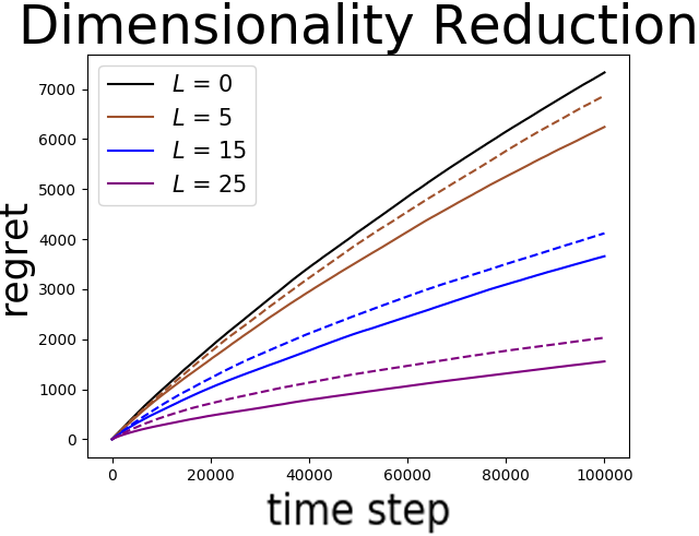
(a) (a)

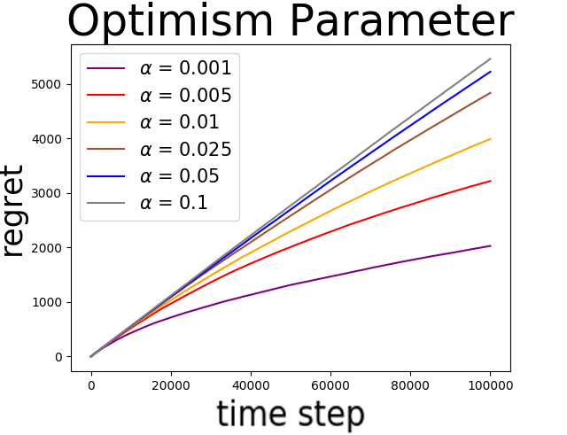
(b) (b)

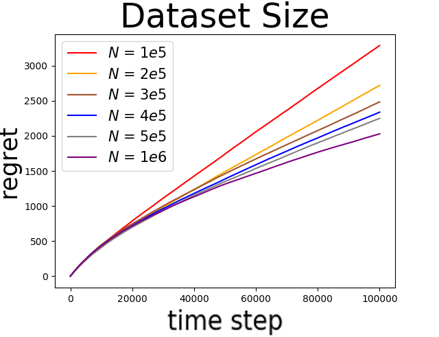
(c) (c)

Figure 3: All experiments were conducted with the same vectors $w^{*}_{a}$ of dimension $d=30$ and $K=30$ arms. (a) Plot compares effect of $L$ when $R_{12}$ is known (solid lines) vs. estimated (dashed lines). For $L=0$ (i.e., no side information) we executed Algorithm 1 without using the dataset. (b) Comparison of different values of $\alpha$ using an offilne dataset and $L=25$. (c) Effect of dataset size on performance for $L=25$.

Algorithm 2 describes the linear bandit variant with partially observable confounded data. Note that, unlike Algorithm 1, Algorithm 2 is not an anytime algorithm, but rather acts knowing the horizon $T$. Assuming $\left\lVert x_{i}\right\rVert_{2}\leq S_{x}$ a.s. and $\left\lVert w_{a}^{*}\right\rVert_{2}\leq S_{w}$ for all $a\in\mathcal{A}$, the algorithm uses an augmented confidence, given by ${\sqrt{\beta_{n,t}(\delta)}=\lambda^{1/2}S_{w}+\left(\sigma+S_{x}S_{w}f_{n}\right)\sqrt{(d-L)\mathrm{log}\left(\frac{1+tS_{x}^{2}/\lambda}{\delta/2\mathrm{log}\left(T\right)K}\right)}}$, where ${f_{n}=f_{B1}+f_{B2}2^{-n/2}}$, $f_{B1}=\widetilde{\mathcal{O}}\left(\max_{a}\frac{\lambda_{\mathrm{min}}\left(R_{11}(a)\right)^{-1}}{P^{\pi_{b}}(a)}S_{x}\left(\text{trace}\left(R_{11}(a)\right)\text{trace}\left(R_{22}(a)\right)\right)^{1/4}\right)$ and $f_{B2}=\widetilde{\mathcal{O}}\left(\max_{a}\frac{\lambda_{\mathrm{min}}\left(R_{11}(a)\right)^{-1}}{P^{\pi_{b}}(a)}S_{x}^{2}\right)$. At every time step $t\in[T]$, the learner uses the estimate $\hat{M}_{t,a}$ and subsequently considers it to be linear side information, as in Algorithm 1. The following theorem provides regret guarantees for Algorithm 2, proving partially observable data can be beneficial for online learning.

Theorem 2.

For any $T>0$, with probability at least $1-\delta$, the regret of Algorithm 2 with the estimator given in Equation (6) is bounded by

$$\text{Regret}(T)\leq 3\sqrt{T(d-L)K\mathrm{log}\left(\lambda+\frac{TS_{x}^{2}}{d-L}\right)}\times$$

$$\left(\sigma_{\epsilon}\sqrt{(d-L)\mathrm{log}\left(\frac{1+TS_{x}^{2}/\lambda}{\delta/(2K\mathrm{log}\left(T\right))}\right)}+\lambda^{1/2}S_{w}\right)+$$

$$\mathcal{O}\left((d-L)\sqrt{K}S_{x}S_{w}f_{B2}\right),$$

where $\epsilon=S_{x}S_{w}f_{B1}$ and $\sigma_{\epsilon}=\sigma+\epsilon$. This leads to, ${\textit{Regret}\left(T\right)\leq\widetilde{\mathcal{O}}\left((1+f_{B_{1}})(d-L)\sqrt{KT}\right).}$

Notice that, unlike Theorem 1, the regret of Algorithm 2 is worsened asymptotically by a factor relating to $f_{B_{1}}$. This function can also scale with $d$, due to its dependence on $\left(\text{trace}\left(R_{11}(a)\right)\right)^{1/4}$ and $\left(\text{trace}\left(R_{22}(a)\right)\right)^{1/4}$. Specifically, a worst case dependence yields ${f_{B_{1}}\leq\widetilde{\mathcal{O}}\left(\max_{a}\frac{\left(L(d-L)\right)^{1/4}}{P^{\pi_{b}}(a)}\right)}$, where here $\max_{a}\frac{1}{P^{\pi_{b}}(a)}\geq K$. That is, $f_{B_{1}}$ is a factor indicating how hard it is to approximate the linear constraints, dependent on the amount of information in $x$ as well as the support of the behavior policy, $\pi_{b}$. Still, in settings in which $d$ and $T$ are prominent over $K$, a significant improvement in performance is achieved.

The proof of the theorem is provided in the supplementary material. Unlike in Theorem 1, we do not have access to the true matrices $M^{\dagger}_{a},P_{a}$, but to increasingly more accurate estimates of these matrices. To deal with this more challenging situation we use the doubling trick. The algorithm acts in exponentially increasing episodes. In each such episode, we fix the estimation of $M_{a}$, i.e., we use the estimate of $M_{a}$ available at the beginning of the episode. The analysis of this algorithm amounts to study the performance of the exact algorithm (as in Theorem 1) up to a fixed, approximated, $M_{a}$, which induces errors in the used $M^{\dagger}_{a},P_{a}$. Finally, summing the regret on each episode, we obtain the result.

The proof heavily relies on the convergence properties of $P_{a},M^{\dagger}$, which are shown to converge at a rate of $O(T^{-1/2})$. These convergence rates are due to the special structure of $M_{a}$. Specifically, we prove that ${\left\lVert P_{a}-\hat{P}_{t,a}\right\rVert\leq 2\left\lVert M_{a}-\hat{M}_{t,a}\right\rVert}$ and ${\left\lVert M_{a}^{\dagger}-\hat{M}_{t,a}^{\dagger}\right\rVert\leq 2\left\lVert M_{a}-\hat{M}_{t,a}\right\rVert}$, meaning, the convergence of $\hat{P}_{t,a}$ and $\hat{M}^{\dagger}_{t,a}$ is well controlled by the convergence of $\hat{M}_{t,a}$. This property does not hold for general matrices. In fact, for a general matrix $A$, $A^{\dagger}$ is not even continuous w.r.t. perturbations in $A$ (see e.g., Stewart 1969). Thus, the structure of $M_{a}$ establishes convergence rates of $\hat{P}_{t,a},\hat{M}^{\dagger}_{t,a}$ sufficient to achieve the desired regret.

Algorithm 2 is highly wasteful w.r.t. the information gathered through time. Specifically, it discards all information upon updates of $\hat{M}_{t,a}$. In a practical setting, we expect the algorithm to achieve similar performance guarantees even when information is not discarded. Moreover, as we show empirically in the next section, significant improvement can still be achieved without applying the doubling trick, i.e., by running Algorithm, 1 with the approximated $\hat{M}_{t,a}$.

6 Experiments

In this section we demonstrate the effectiveness of using offline data in a synthetic environment. Our environment consisted of $K=30$ arms and vectors $w^{*}_{a}\in\mathbb{R}^{30}$ uniformly sampled in $\brk[s]*{0,\frac{1}{d}}^{d}$ and fixed across all experiments. Contexts were sampled from a uniform distribution in $\brk[s]*{0,1}^{d}$ and normalized to have norm $1$. The behavioral policy $\pi_{b}$ was chosen to follow a softmax distribution $\pi_{b}(a,x)\propto\exp\left(\phi_{a}^{T}x\right)$, where $\phi_{a}\in\mathbb{R}^{d}$ were randomly chosen and fixed across all experiments.

Figure 3a illustrates the effectiveness of using partially observable data. We used a dataset of $1$ million examples to simulate a sufficiently large dataset. Solid lines depict regret when $R_{12}(a)$ are known in advance, allowing us to apply Algorithm 1 without estimations (Section 4). Dashed lines depict regret for the estimated case using queries to $\pi_{b}$, i.e., $M_{a}$ were estimated at every iteration using an estimate of $R_{12}(a)$ (see Section 5). Note that $L=0$ corresponds to the linear bandit problem with no side information, i.e., the original OFUL algorithm. It is evident that utilizing the partially observable data can significantly improve performance, even when using approximate projections. We note that the experiments were run under constant updates of $\hat{M}_{t,a}$, i.e., without epoch schedules.

Figure 3b depicts the effect of the optimism parameter $\alpha$ (see Algorithm 1) on overall performance when utilizing a dataset with $L=25$ observed features. A gap is evident between the proposed theoretical confidence and the practical results, as very small values of $\alpha$ showed best performance. This gap is most likely due to worst case scenarios that were not imposed by our simulated environments.

Finally, Figure 3c depicts experiments with varying amount of data. While the number of examples has an effect, it does not significantly deteriorate overall performance, suggesting that partially observable offline data can be used even with finite datasets, as long as they are sufficiently large.

7 Related Work

The linear bandits problem, first introduced by Auer [2002], has been extensively investigated in the pure online setting [Dani et al., 2008, Rusmevichientong and Tsitsiklis, 2010, Abbasi-Yadkori et al., 2011], with numerous variants and extensions [Agrawal and Devanur, 2016, Kazerouni et al., 2017, Amani et al., 2019].

The offline (logged) bandit setting usually assumes the algorithm must learn a policy from a batch of fully observable data [Shivaswamy and Joachims, 2012, Swaminathan and Joachims, 2015, Joachims et al., 2018]. The use of offline data has also been investigated under the reinforcement learning framework, including batch-mode off-policy reinforcement learning and off-policy evaluation [Ernst et al., 2005, Lizotte et al., 2012, Fonteneau et al., 2013, Precup, 2000, Thomas and Brunskill, 2016, Gottesman et al., 2019b]

More related to our work are attempts to establish unbiased estimates or control schemes from confounded offline data [Lattimore et al., 2016, Oberst and Sontag, 2019, Tennenholtz et al., 2020]. Other work in which partially observable data is used usually consider the standard confounded setting (e.g., identification of $P(r|\text{do}(a))$) [Zhang and Bareinboim, 2019, Ye et al., 2020]. Wang et al. [2016] also consider hidden features, where biases are accounted for under assumptions on the hidden features. In these works the unobserved features (confounders) are never disclosed to the learner. Prior knowledge is thereby usually assumed over their support (e.g., known bounds). When such priors are unknown, these methods may thus fail. Moreover, they are sub-optimal in settings of fully observable interactions, where unobserved confounders become observed covariates.

In this work we view the problem from an online learner’s perspective, where offline data is used as side information. Specifically we project the given information, reducing our problem to its orthogonal subspace. Projections have been previously used in the bandit setting for reducing time complexity and dimensionality [Yu et al., 2017]. Other work consider bandits under constraints [Agrawal and Devanur, 2019]. Finally, Djolonga et al. [2013] consider subspace-learning by combining Gaussian Process UCB sampling and low-rank matrix recovery techniques.

8 Discussion and Future Work

In this work we showed that partially observable confounded data can be efficiently utilized in the linear bandit setting. In this section we further discuss two central assumptions made in our work; namely, infinite data and bounding the cross correlation matrix $R_{12}$.

Finite Data. Throughout our work we assumed the limit of infinite sized data. From a technical perspective, the use of finite data would introduce an error in the least squares estimator [Krikheli and Leshem, 2018]. A straightforward analysis would propagate this error as additional linear penalty to the regret that is dependent on the number of samples in the data. More involved techniques may combine optimistic bounds on the finite samples in the data. We chose to leave its derivation out to focus on the topic of missing covariates in the data. Finally, our experiments demonstrate that the number of samples does not greatly affect performance, as long as they are sufficiently large, i.e., when the error is small relative to $T$.

Bounding $R_{12}$. Being able to estimate $R_{12}(a)$ is an essential requirement for deconfounding the partially observable data. Nevertheless, $R_{12}(a)$ is dependent on $\pi_{b}$, raising the question, can $R_{12}(a)$ be estimated without knowledge of $\pi_{b}$? In our work we showed how one can estimate it using queries to $\pi_{b}$. In fact, we did not require knowledge of $\pi_{b}$, nor did we require interactions of $\pi_{b}$ with the environment (i.e., we do not act according to $\pi_{b}$), but rather, only view samples from $\pi_{b}$. While such an assumption may be strict in some settings, it is reasonable in others. For instance, when $\pi_{b}$ was controlled by us when the data was recorded. Other settings for estimating $R_{12}(a)$ are also possible, e.g., having access to additional fully observable datasets that were generated by $\pi_{b}$ [Kallus et al., 2018].

Consider the examples of the healthcare and traffic management settings presented in Section 1. In the medical setting, quering $\pi_{b}$ would amount to asking the clinician that induced the data what she would have done in a provided situation. In this scenario, cooperation of the clinician is needed to deconfound the data. Nevertheless, note that this approach is not limited by the amount of confounding bias inherent in the data, allowing us identify optimal control policies. Unlike the medical example, in the traffic management example we have access to the behavior policy that generated the data. In this scenario, the querying assumption is insignificant.

Future Work. While this work assumed a monotonically vanishing error of $\hat{R}_{12}(a)$ (i.e., asymptotic identifiability), future work can consider looser bounds on the estimate. It is also interesting to understand the contextual bandit algorithms, both in the linear as well as the general function class settings. It is also interesting to generalize our results to the reinforcement learning setting.

Appendices

1. 1 Introduction
2. 2 Problem Setting
3. 3 From Partially Observable Offline Data to Linear Side Information
   1. 3.1 Linear Side Information
4. 4 Linear Contextual Bandits with Linear Side Information
5. 5 Deconfounding Partially Observable Data
   1. 5.1 Case Study: Queries to $\pi_{b}$
6. 6 Experiments
7. 7 Related Work
8. 8 Discussion and Future Work
9. Appendix A Overview
10. Appendix B Orthogonal Projections and the Moore–Penrose Inverse
    1. B.1 Useful Perturbation Bounds
11. Appendix C Unidentifiability Problem of Partially Observable Data
12. Appendix D Proof of Proposition 1
13. Appendix E Linear Regression with Side Information
14. Appendix F OFUL with Linear Side Information
    1. F.1 Equivalences of Update Rule
    2. F.2 Proof of Theorem 1
    3. F.3 Optimism of OFUL
15. Appendix G OFUL with Learned Subspace
    1. G.1 Notations and the Good Event of Theorem 2
    2. G.2 Proof of Theorem 2
    3. G.3 Optimism of OFUL with Learned Subspace
16. Appendix H Convergence of $M,M^{\dagger},P$
17. Appendix I Useful Results

Appendix A Overview

The appendix is orginized as follows:

• Appendix B provides a short background on orthogonal projections and the Moore-Penrose inverse, a fundamental tool in our work. We also state some well known pertrubations bounds that will be useful for achieving well-behaved convergence rates in the proof of Theorem 2.

• In Appendix C we discuss the unidentifiability problem of using partially observable data, with focus to our setting. Specifically, we show that $\brk[c]*{w_{a}^{*}}_{a\in\mathcal{A}}$ are not identifiable, and provide further motivation for this work.

• Appendix D provides a proof of Proposition 1, namely, showing that the structure of the transformation obtained from the offline data is given by $M_{a}=(I_{L},R_{11}(a)^{-1}R_{12}(a))$.

• In Appendix E we discuss Projected Ridge Regression (P-RR) with side information, as presented in Section 4. Specifically, we state and prove the equivalence of P-RR to a low-order ridge regression problem with a correction term (see Equation (4)).

• Appendix F provides a proof of Theorem 1, showing that Algorithm 1 reduces the OFUL algorithm to the lower-dimensional projected subspace of known linear transformation $\brk[c]*{M_{a}w=b_{a}}$, decreasing the regret from $\widetilde{\mathcal{O}}\left(d\sqrt{KT}\right)$ to $\widetilde{\mathcal{O}}\left((d-L)\sqrt{KT}\right)$. Its proof is a direct consequence of the P-RR formulation.

• Based on the above, we formulate our final result, proving Theorem 2 in Appendix G. We begin by showing the approximate linear transformations obtained by estimating $R_{12}(a)$ from online samples are well behaved. Specifically, we show that the projection and pseudo-inverse operators converge at the same rate as $\hat{M}_{t,a}$, i.e., $\left\lVert P_{a}-\hat{P}_{t,a}\right\rVert\leq 2\left\lVert M_{a}-\hat{M}_{t,a}\right\rVert$ and $\left\lVert M_{a}^{\dagger}-\hat{M}_{t,a}^{\dagger}\right\rVert\leq 2\left\lVert M_{a}-\hat{M}_{t,a}\right\rVert$. We then leverage these important properties, together with a doubling trick approach, showing that similar regret guarantees can be achieved as in the exact case.

Appendix B Orthogonal Projections and the Moore–Penrose Inverse

In this section we give a short review of the Moore–Penrose inverse [Barata and Hussein, 2012] and its corresponding orthogonal projection. We state some well known properties that will be useful in our analysis.

For a matrix $M\in\mathbb{R}^{L\times d}$ we denote its Moore–Penrose inverse by $M^{\dagger}$. Let $P^{\mathbin{\|}}=M^{\dagger}M$ be the orthogonal projection onto the range of $M$ and $P^{\bot}=I-P^{\mathbin{\|}}$ be the orthogonal projection onto the kernel of $M$. We have the following well known properties.

Property 1.

If $M$ has independent rows, then $M^{\dagger}$ can be computed as $M^{\dagger}=M^{T}(MM^{T})^{-1}.$

Property 2.

If $Mw=b$ then $P^{\mathbin{\|}}w=M^{\dagger}b$.

Property 3 (Planitz 1979).

The vector $x=M^{\dagger}b$ is the vector with the smallest $L_{2}$ norm which satisfies $Mx=b$.

Property 4.

If $w\in\mathbb{R}^{d}$ satisfies $Mw=b$ then $w$ can be written as

$$w=P^{\bot}w+M^{\dagger}b.$$

Proof.

Using the fact $I=P^{\mathbin{\|}}w+P^{\bot}$ and Property 2 we get

$$w=P^{\bot}w+P^{\mathbin{\|}}w=P^{\bot}w+M^{\dagger}b.$$

∎

Remark 1 (Notation).

For brevity, we denote $P=P^{\bot}$ as the orthogonal projection to the kernel of $M$ and $I-P=I-P^{\bot}=P^{\mathbin{\|}}$ as the orthogonal projection to the range of $M$.

B.1 Useful Perturbation Bounds

The following two results are standard in perturbation theory. They bound the $L_{2}$ difference between some matrix $A$, and its perturbed counterpart $B=A+E$, where $E$ a perturbation (i.e., error) matrix.

Theorem 3 (E.g., Chen et al. 2016, Corollary 2.7).

For any matrices let $A,B,E\in\mathbb{R}^{d\times d}$ and $E=B-A$. Let $P_{A}$ and $P_{B}$ be the orthogonal projection on the raw space of $A$ and $B$, respectively. Assume ${\mathrm{rank}}(A)={\mathrm{rank}}(B)$. Then,

$$\left\lVert P_{A}-P_{B}\right\rVert_{2}\leq\min\left(\left\lVert A^{\dagger}\right\rVert_{2},\left\lVert B^{\dagger}\right\rVert_{2}\right)\left\lVert E\right\rVert_{2},$$

where $P,\hat{P}$ are the orthogonal projections into the row space of $M,\hat{M}$, respectively,

Theorem 4 (Stewart 1977, Theorem 3.3).

For any matrices let $A,B,E\in\mathbb{R}^{d\times d}$ and $E=B-A$. Then,

$$\left\lVert B^{\dagger}-A^{\dagger}\right\rVert_{2}\leq 2\max\left(\left\lVert A^{\dagger}\right\rVert^{2}_{2},\left\lVert B^{\dagger}\right\rVert^{2}_{2}\right)\left\lVert E\right\rVert_{2}.$$

Remark 2.

Note that Theorem 3 assumes ${\mathrm{rank}}(A)={\mathrm{rank}}(B)$. While other perturbation bounds exist for the case ${\mathrm{rank}}(A)\neq{\mathrm{rank}}(B)$, they do not provide sufficient guarantees for our analysis (e.g., $\left\lVert A^{\dagger}-B^{\dagger}\right\rVert$ may diverge Stewart 1969). Luckily, due to the special structure of $M$, i.e., $M=(I_{L},R_{11}^{-1}R_{12})$, the perturbed version of $M$ as defined in Section 5 will always have rank $L$, ensuring this assumption holds.

Appendix C Unidentifiability Problem of Partially Observable Data

Having access to partially observable offline data may not be enough to obtain the optimal policy, even if $N\to\infty$. The following is a standard identifiability result, showing that $\brk[c]*{w_{a}^{*}}_{a\in\mathcal{A}}$ are not identifiable in the setting of partially observable data and no online interaction.

Proposition 2.

For any behavioral policy $\pi_{b}$ and induced measure $P^{\pi_{b}}$, $\brk[c]*{w_{a}^{*}}_{a\in\mathcal{A}}$ are not identifiable. More specifically, for all $w^{1}=\brk[c]*{w_{a}^{1}}_{a\in\mathcal{A}}$ exist $w^{2}=\brk[c]*{w_{a}^{2}}_{a\in\mathcal{A}}\neq w^{2}$ and probability measures $P_{1},P_{2}$ such that ${P_{1}\left(x^{\mathrm{o}},a,r;w^{1},\pi_{b}\right)=P_{2}\left(x^{\mathrm{o}},a,r;w^{2},\pi_{b}\right)}$ and $\pi_{b}\left(a,x;w^{1}\right)=\pi_{b}\left(a,x;w^{2}\right)$.

Proof.

Denote by $w^{o}_{a}\in\mathbb{R}^{L},w^{h}_{a}\in\mathbb{R}^{d-L}$, the vectors corresponding to the observed and hidden parts of $x$, namely, $x^{\mathrm{o}}$ and $x^{\mathrm{h}}$, respectively. That is, $w_{a}=\begin{pmatrix}w^{o}_{a}\\ w^{h}_{a}\end{pmatrix}$ and

$$r_{i}=x_{i}^{T}w_{a}+\eta_{i}=(x^{\mathrm{o}})^{T}w^{o}_{a}+(x^{\mathrm{h}})^{T}w^{h}_{a}+\eta_{i}.$$

Let $P_{1},P_{2}$ be two measures such that $P_{1}((x^{\mathrm{h}})^{T}w^{1o}_{a}\leq\alpha|a,x^{\mathrm{o}})=P_{2}((x^{\mathrm{h}})^{T}w^{2o}_{a}\leq\alpha|a,x^{\mathrm{o}})$ for all $\alpha\in\mathbb{R}$. Note that such measures always exist. For example letting $x^{\mathrm{h}}$ be a random vector with i.i.d. elements independent of $x^{\mathrm{o}}$, such that

$$\begin{cases}&P_{1}\left((x^{\mathrm{h}})_{k}=\frac{1}{(w^{1o}_{a})_{k}}\right)=\frac{1}{2}\\ &P_{1}\left((x^{\mathrm{h}})_{k}=\frac{1}{(w^{2o}_{a})_{k}}\right)=0\\ &P_{1}\left(x^{\mathrm{h}})_{k}=0\right)=\frac{1}{2}\end{cases}\qquad\begin{cases}&P_{2}\left((x^{\mathrm{h}})_{k}=\frac{1}{(w^{1o}_{a})_{k}}\right)=0\\ &P_{2}\left((x^{\mathrm{h}})_{k}=\frac{1}{(w^{2o}_{a})_{k}}\right)=\frac{1}{2}\\ &P_{2}\left(x^{\mathrm{h}})_{k}=0\right)=\frac{1}{2}\end{cases}$$

where without loss of generality we assumed $(w^{1o}_{a})_{k}\neq 0,(w^{2o}_{a})_{k}\neq 0,\forall 1\leq k\leq d-L$ . Then it follows that $P_{1}((x^{\mathrm{h}})^{T}w^{1o}_{a}\leq\alpha|a,x^{\mathrm{o}})=P_{2}((x^{\mathrm{h}})^{T}w^{2o}_{a}\leq\alpha|a,x^{\mathrm{o}})$.

We have that

$$P_{1}(r\leq\beta|a=a,x^{\mathrm{o}}=c;w^{1},\pi_{b}) =P_{1}((x^{\mathrm{h}})^{T}w^{o}_{a}+\eta\leq\beta-c^{T}w^{o}_{a}|a=a,x^{\mathrm{o}}=c;w^{1},\pi_{b})$$

$$=P_{2}(r\leq\beta|a=a,x^{\mathrm{o}}=c;w^{2},\pi_{b}).$$

Therefore,

$$P_{1}(r,a,x^{\mathrm{o}};w^{1},\pi_{b}) =P_{1}(r|a,x^{\mathrm{o}};w^{1},\pi_{b})P^{\pi_{b}}(a,x^{\mathrm{o}})$$

$$=P_{2}(r|a,x^{\mathrm{o}};w^{2},\pi_{b})P^{\pi_{b}}(a,x^{\mathrm{o}})$$

$$=P_{2}(r,a,x^{\mathrm{o}};w^{2},\pi_{b}).$$

∎

The above proposition tells us that partially observable offline data cannot be used unless further assumptions are made. This is true even in the linear model, which is the focus of this work. To mitigate this problem, prior knowledge and assumptions over the hidden variables can be used. Nevertheless, such assumptions may be inaccurate and impossible to validate. Moreover, most concurrent assumptions (such as bounding the “amount of confoundness"), do not completely resolve this issue, but rather mitigate it so that perhaps better policies can be found.

This work considers an alternative assumption, namely, access to online interactions with the environment. This has several benefits over assuming prior knowledge:

1. There is no problem of validating this assumption, i.e., if we do not have access to an online environment, we will know it.

2. The online regime allows us to achieve an optimal policy. Specifically, since online interactions reveal the hidden context, an optimal policy is always identifiable.

3. Partially observable data cannot hurt us, but rather only improve our performance. Looking at the problem from an online learner’s point of view, the offline data is only used to improve its performance. Therefore, the offline data does not bias our results, but only decreases the number of online interactions.

Appendix D Proof of Proposition 1

We recall Proposition 1 See 1

Before proving the proposition, we remind the reader of the continuous mapping theorem, which states that continuous functions preserve limits even if their arguments are sequences of random variables.

Theorem 5 (Continuous Mapping, e.g., [Van der Vaart, 2000]).

Let $\left\{X_{n}\right\}$ be a set of real random variables such $X_{n}\in\mathbb{R}^{k}$ and $X_{n}\overset{a.s}{\rightarrow}X$. Let $d(\cdot,\cdot):\mathbb{R}^{d}\times\mathbb{R}^{d}\rightarrow\mathbb{R}$ be a distance function that generates the usual topology. Let $g:\mathbb{R}^{k}\rightarrow\mathbb{R}^{m}$ be a continuous function at the point $X\in\mathbb{R}^{k}.$ Then $g(X_{n})\overset{a.s}{\rightarrow}g(X)$.

Proof of Proposition 1.

Fix $a\in\mathcal{A}$. By definition, $b^{LS}_{a}$ is also given by (1),

$$b^{LS}_{a} =\left(\frac{1}{N_{a}}\sum_{n\in[N]}\mathbbm{1}_{\brk[c]*{a_{n}=a}}x^{\mathrm{o}}_{n}\left(x^{\mathrm{o}}_{n}\right)^{T}\right)^{-1}\left(\frac{1}{N_{a}}\sum_{n\in[N]}\mathbbm{1}_{\brk[c]*{a_{n}=a}}x^{\mathrm{o}}_{n}r_{n}\right),$$ (7)

Define $\left(Q^{\mathrm{o}}\right)^{T}=\begin{pmatrix}I_{L}&0\end{pmatrix}\in\mathbb{R}^{L\times d}$ and $\left(Q^{\mathrm{c}}\right)^{T}=\begin{pmatrix}0&I_{d-L}\end{pmatrix}\in\mathbb{R}^{d-L\times d}$. Observe that $x^{\mathrm{o}}=Q^{\mathrm{o}}x$, $x^{\mathrm{h}}=Q^{\mathrm{c}}x$ for $x\in\mathbb{R}^{d},$ and that $I_{d}=Q^{\mathrm{o}}\left(Q^{\mathrm{o}}\right)^{T}+Q^{\mathrm{c}}\left(Q^{\mathrm{c}}\right)^{T}.$ Due to the model assumption (see Section 2), we can write

$$r(x_{n},a) =\brk[a]*{x_{n},w^{*}_{a}}+\eta_{n}$$

$$=\brk[a]*{Q^{\mathrm{o}}\left(Q^{\mathrm{o}}\right)^{T}x_{n},w^{*}_{a}}+\brk[a]*{Q^{\mathrm{c}}\left(Q^{\mathrm{c}}\right)^{T}x_{n},w^{*}_{a}}+\eta_{n} Q^{\mathrm{o}}\left(Q^{\mathrm{o}}\right)^{T}+Q^{\mathrm{c}}\left(Q^{\mathrm{c}}\right)^{T}=I$$ ()

$$=\brk[a]*{x^{\mathrm{o}}_{n},(Q^{\mathrm{o}})^{T}w^{*}_{a}}+\brk[a]*{x^{\mathrm{h}}_{n},(Q^{\mathrm{c}})^{T}w^{*}_{a}}+\eta_{n}$$

Plugging this relation into (1) we get

$$b_{a}^{LS}= \left(\frac{1}{N_{a}}\sum_{n\in[N]}\mathbbm{1}_{\brk[c]*{a_{n}=a}}x^{\mathrm{o}}_{n}\left(x^{\mathrm{o}}_{n}\right)^{T}\right)^{-1}\left(\frac{1}{N_{a}}\sum_{n\in[N]}\mathbbm{1}_{\brk[c]*{a_{n}=a}}x^{\mathrm{o}}_{n}\left(x^{\mathrm{o}}_{n}\right)^{T}\right)\left(Q^{\mathrm{o}}\right)^{T}w^{*}_{a}$$

$$+\left(\frac{1}{N_{a}}\sum_{n\in[N]}\mathbbm{1}_{\brk[c]*{a_{n}=a}}x^{\mathrm{o}}_{n}\left(x^{\mathrm{o}}_{n}\right)^{T}\right)^{-1}\left(\frac{1}{N_{a}}\sum_{n\in[N]}\mathbbm{1}_{\brk[c]*{a_{n}=a}}x^{\mathrm{o}}_{n}\left(x^{\mathrm{h}}_{n}\right)^{T}\right)\left(Q^{\mathrm{c}}\right)^{T}w^{*}_{a}$$

$$+\left(\frac{1}{N_{a}}\sum_{n\in[N]}\mathbbm{1}_{\brk[c]*{a_{n}=a}}x^{\mathrm{o}}_{n}\left(x^{\mathrm{o}}_{n}\right)^{T}\right)^{-1}\left(\frac{1}{N_{a}}\sum_{n\in[N]}\mathbbm{1}_{\brk[c]*{a_{n}=a}}x^{\mathrm{o}}_{n}\eta_{n}\right).$$ (8)

We now analyze the three terms and apply the continuous mapping theorem iteratively (Theorem 5) to prove the lemma. Let

$$Y^{(i)}_{N}\coloneqq\frac{1}{N_{a}}\sum_{n\in[N]}\mathbbm{1}_{\brk[c]*{a_{n}=a}}x^{\mathrm{o}}_{n}\left(x^{\mathrm{o}}_{n}\right)^{T}=\frac{1}{N_{a}/N}\frac{1}{N}\sum_{n\in[N]}\mathbbm{1}_{\brk[c]*{a_{n}=a}}x^{\mathrm{o}}_{n}\left(x^{\mathrm{o}}_{n}\right)^{T}=\frac{Z_{N}^{(2)}}{Z_{N}^{(1)}},$$ (9)

where $Z_{N}^{(1)}\coloneqq N_{a}/N=\frac{1}{N}\sum_{n\in[N]}\mathbbm{1}_{\brk[c]*{a_{n}=a}}$ and $Z_{N}^{(2)}\coloneqq\frac{1}{N}\sum_{n\in[N]}\mathbbm{1}_{\brk[c]*{a_{n}=a}}x^{\mathrm{o}}_{n}\left(x^{\mathrm{o}}_{n}\right)^{T}.$

By the strong law of large numbers (SLLN)

$$Z_{N}^{(1)}\overset{a.s}{\rightarrow}P^{\pi_{b}}(a)$$

$$Z_{N}^{(2)}\overset{a.s}{\rightarrow}P^{\pi_{b}}(a)\mathbb{E}^{#1}\left[x^{\mathrm{o}}\left(x^{\mathrm{o}}\right)^{T}\mid a\right]$$

for $N\rightarrow\infty$ since both are empirical averages of $N$ i.i.d. random variables and, thus, converge to their means a.s..

The mean of a random variable in the empirical average $Z_{N}^{(1)}$ is simply given by

$$\mathbb{E}^{#1}\left[\mathbbm{1}_{\brk[c]*{a_{n}=a}}\right]=P^{\pi_{b}}(a)$$

since all the random variables are i.i.d..

The mean of a random variable in the empirical average of $Z_{N}^{(2)}$ is given by

since $\mathbb{E}^{#1}\left[X\mid A\right]=\frac{\mathbb{E}^{#1}\left[\mathbbm{1}_{\brk[c]*{A}}X\right]}{P(A)}$.

By the continuous mapping theorem (Theorem 5) we get that

$$Y^{(i)}_{N}\overset{a.s}{\rightarrow}\frac{P^{\pi_{b}}(a)\mathbb{E}^{#1}\left[x^{\mathrm{o}}\left(x^{\mathrm{o}}\right)^{T}\mid a\right]}{P^{\pi_{b}}(a)}=\mathbb{E}^{#1}\left[x^{\mathrm{o}}\left(x^{\mathrm{o}}\right)^{T}\mid a\right],$$

which is valid since $g(a,b)=\frac{a}{b}$ is continuous at $b>0$ and we assume that for all $a\in\mathcal{A}$ $P^{\pi_{b}}(a)>0.$

Similar reasoning, leads to the following convergence and

$$Y^{(iii)}_{N}\coloneqq\frac{1}{N_{a}}\sum_{n\in[N]}\mathbbm{1}_{\brk[c]*{a_{n}=a}}x^{\mathrm{o}}_{n}\eta_{n}\overset{a.s}{\rightarrow}0,$$ (10)

where in the last relation we also use the fact that $\eta_{n}$ is zero mean random variable, $\mathbb{E}^{#1}\left[\eta_{n}\right]=0$, and is independent of $x_{n},a_{n}$ and thus $\eta_{n}$ is also independent of $x^{\mathrm{o}}_{n}=Q^{\mathrm{o}}x_{n},a_{n}$.

By (8) and by definitions (9), (LABEL:eq:_Yb_supp), (10),

$$b_{a}^{LS}=(Y^{(i)}_{N})^{-1}Y^{(i)}_{N}Q^{\mathrm{o}}w^{*}_{a}+(Y^{(i)}_{N})^{-1}Y^{(ii)}_{N}Q^{\mathrm{c}}w^{*}_{a}+(Y^{(i)}_{N})^{-1}Y^{(iii)}_{N}.$$

We now apply the continuous mapping theorem (Theorem 5) on each of the three terms. Notice that the conditions of this theorem are satisfied since the limit of $Y^{(i)}_{N}$, $\mathbb{E}^{#1}\left[x^{\mathrm{o}}\left(x^{\mathrm{o}}\right)^{T}\mid a\right]$, has an inverse by the assumption which implies that the limit point is continuous. Thus, we get that for $N\rightarrow\infty$ it holds a.s. that

$$b_{a}^{LS}=\left(Q^{\mathrm{o}}\right)^{T}w_{a}^{*}+R_{11}(a)^{-1}R_{12}(a)\left(Q^{\mathrm{c}}\right)^{T}w_{a}^{*}$$

where $R_{11}(a)=\mathbb{E}^{#1}\left[\nonscript\,x^{\mathrm{o}}\left(x^{\mathrm{o}}\right)^{T}\nonscript\;\middle|\nonscript\>\allowbreak a\nonscript\,\right],\ R_{12}(a)=\mathbb{E}^{#1}\left[\nonscript\,x^{\mathrm{o}}\left(x^{\mathrm{h}}\right)^{T}\nonscript\;\middle|\nonscript\>\allowbreak a\nonscript\,\right].$ By taking union bound on all $a\in\mathcal{A}$ we conclude the proof. ∎

Appendix E Linear Regression with Side Information

We wish to construct a least squares variant for $w^{*}_{a}$, which utilizes the information in Equation (2). In Section 4 we considered the problem of linear regression under the linear model ${y=\brk[a]*{x,Pw^{*}}+\eta}$, where $P\in\mathbb{R}^{d\times d}$ is a projection matrix of rank $m$ and $\eta$ is some centered random noise. One way to solve this problem is through ridge regression on the full euclidean space $\mathbb{R}^{d}$, under projection of $w$. In Section 4 we constructed a projected variant of ridge regression (P-RR), which attempts to solve the regularized problem in Equation 4, i.e.,

$$\min_{w\in\mathbb{R}^{d}}\brk[c]*{\sum_{i=1}^{t-1}\left(\brk[a]*{x_{i},P_{a}w}-y_{a,i}\right)^{2}+\lambda\left\lVert P_{a}w\right\rVert_{2}^{2}},$$

We then took its smallest norm solution

$$\hat{w}_{t,a}^{P_{a}}=\left(P_{a}\left(\lambda I_{d}+\sum_{i=1}^{t-1}x_{i}x_{i}^{T}\right)P_{a}\right)^{\dagger}\left(\sum_{i=1}^{t-1}y_{i}x_{i}\right).$$ (11)

where $y_{a,i}=r_{i}-\brk[a]*{x_{i},M_{a_{i}}^{\dagger}b_{a_{i}}}$.

Let us now take a closer look at Equation (11). We wish to show that this solution is closely related to a ridge regression problem in a lower dimension. First, notice that taking the pseudoinverse of $P_{a}\left(\lambda I_{d}+\sum_{i=1}^{t-1}x_{i}x_{i}^{T}\right)P_{a}$ can be written in an equivalent method using the inverse operator. This is formalized generally in the following proposition.

Proposition 3.

Let $V\in\mathbb{R}^{d\times d}$ be a PD matrix and $P=UU^{T}$ a projection matrix of rank $l$, where and $U\in\mathbb{R}^{d\times l}$ is a matrix with orthonormal columns. Then,

$$(PVP)^{\dagger}=U(U^{T}VU)^{-1}U^{T}.$$

Proof.

Observe that

$$PVP=U(U^{T}VU)U^{T}$$ (12)

Let $U_{\mathrm{Ext}}\in\mathbb{R}^{d\times d}$ be a unitary matrix with its first $l$ columns $U$ and rest $d-l$ columns be arbitrary orthonormal vectors (such that $U_{\mathrm{Ext}}$ is unitary), i.e., an extension of $U$ to the entire space $\mathbb{R}^{d}$. Using this notation (12) can be written as

$$PVP=U_{\mathrm{Ext}}\begin{pmatrix}U^{T}VU&0\\ 0&0\end{pmatrix}U_{\mathrm{Ext}}^{T}.$$ (13)

Next, recall that for any unitary matrix $\bar{U}$ and any matrix $A$ it holds that $(\bar{U}A\bar{U}^{T})^{\dagger}=\bar{U}A^{\dagger}\bar{U}^{T}$. Then, by Equation (13)

$$\left(PVP\right)^{\dagger} =\left(U_{\mathrm{Ext}}\begin{pmatrix}U^{T}VU&0\\ 0&0\end{pmatrix}U_{\mathrm{Ext}}^{T}\right)^{\dagger}$$

$$=U_{\mathrm{Ext}}\begin{pmatrix}U^{T}VU&0\\ 0&0\end{pmatrix}^{\dagger}U_{\mathrm{Ext}}^{T}$$

$$=U_{\mathrm{Ext}}\begin{pmatrix}(U^{T}VU)^{\dagger}&0\\ 0&0\end{pmatrix}U_{\mathrm{Ext}}^{T}$$

$$=U_{\mathrm{Ext}}\begin{pmatrix}(U^{T}VU)^{-1}&0\\ 0&0\end{pmatrix}U_{\mathrm{Ext}}^{T}=U(U^{T}VU)^{-1}U^{T},$$ (14)

where the third relation holds since $U^{T}VU$ is full rank (since $V$ is PD so is $U^{T}VU$). ∎

Using Proposition 3 we now show that P-RR is in fact equivalent to solving a ridge regression problem in a lower dimension. This will become useful in our proof of Theorem 1, as it will allow us to reduce the linear bandit problem to a lower dimensional variant of the same problem. The following proposition proves this equivalence.

Proposition 4 (Equivalent forms of P-RR).

Let $w_{\mathrm{PRR}}\in\mathbb{R}^{d}$ be the least $L_{2}$-norm solution of the following P-RR for $\lambda>0$

$$\arg\min_{w\in\mathbb{R}^{d}}\left(\sum_{n=1}^{t}\left(\brk[a]*{Px_{n},w}-y_{n}\right)^{2}+\lambda\left\lVert Pw\right\rVert_{2}^{2}\right),$$

where $x_{n}\in\mathbb{R}^{d},y_{n}\in\mathbb{R}$, $P=UU^{T}$ is a projection matrix of rank $l$ and $U\in\mathbb{R}^{d\times l}$ is a matrix with orthonormal columns. Define $X\in\mathbb{R}^{t\times d}$ and $\tilde{X}\in\mathbb{R}^{t\times l}$ as matrices with $\left\{x_{n}^{T}\right\}_{n=1}^{t}$ and $\left\{(U^{T}x_{n})^{T}\right\}_{n=1}^{t}$ in their rows, respectively. Define $Y\in\mathbb{R}^{t}$ as the vector of $\left\{y_{n}\right\}_{n=1}^{t}$. Then, $w_{\mathrm{PRR}}$ satisfies the following relations.

1. $w_{\mathrm{PRR}}=(P(X^{T}X+\lambda I_{d})P)^{\dagger}PX^{T}Y$.

2. $U^{T}w_{\mathrm{PRR}}=(\tilde{X}^{T}\tilde{X}+\lambda I_{l})^{-1}\tilde{X}^{T}Y.$

Proof.

Claim (1). The P-RR problem can we recast as

$$\arg\min_{w\in\mathbb{R}^{d}}\left(w^{T}(P(X^{T}X+\lambda I_{d})P)w+2w^{T}PX^{T}Y\right).$$

The smallest $L_{2}$ norm solution of this optimization problem is given by

$$w_{\mathrm{PRR}}=(P(X^{T}X+\lambda I_{d})P)^{\dagger}PX^{T}Y$$ (15)

which establishes the first claim.

Claim (2).

By Proposition 3 it holds that

$$(P(X^{T}X+\lambda I_{d})P)^{\dagger}=U(U^{T}(X^{T}X+\lambda I_{d})U)^{-1}U^{T}$$

$$=U(U^{T}X^{T}XU+\lambda I_{l})^{-1}U^{T} U^{T}U=I_{l}$$ ()

$$=U(\tilde{X}^{T}\tilde{X}+\lambda I_{l})^{-1}U^{T},$$ (16)

by defining $\tilde{X}=XU$, which is a matrix with $\left\{U^{T}x_{n}\right\}$ in its rows. To conclude the proof, observe the following holds

$$U^{T}w_{\mathrm{PRR}} =U^{T}\left(U(\tilde{X}^{T}\tilde{X}+\lambda I_{l})^{-1}U^{T}\right)PX^{T}Y$$ (By (15) and (16))

$$=U^{T}U(\tilde{X}^{T}\tilde{X}+\lambda I_{l})^{-1}U^{T}U\tilde{X}^{T}Y$$

$$=(\tilde{X}^{T}\tilde{X}+\lambda I_{l})^{-1}\tilde{X}^{T}Y. U^{T}U=I_{l}$$ ()

∎

Appendix F OFUL with Linear Side Information

Algorithm 3 OFUL with Linear Side Information (Equivalent Form)

1:input: $\alpha>0,M_{a}\in\mathbb{R}^{L\times d},b_{a}\in\mathbb{R}^{L}$

2:init: $V_{a}=\lambda I,Y_{a}=0,\forall a\in\mathcal{A}$

3:for $t=1,\ldots,T$ do

4:   Receive context $x_{t}$

5:   ${\hat{w}_{t,a}^{P_{a}}=\left(P_{a}V_{a}P_{a}\right)^{\dagger}\left(Y_{a}-\left(V_{a}-\lambda I\right)M_{a}^{\dagger}b_{a}\right)}$

6:   ${\sqrt{\beta_{t}(\delta)}=\sigma\sqrt{(d-L)\mathrm{log}\left(\frac{K(1+tS_{x}^{2}/\lambda)}{\delta}\right)}+\lambda^{1/2}S_{w}}$

7:   $a_{t},\tilde{w}_{t,a_{t}}\in\arg\max_{a\in\mathcal{A},w_{a}\in C_{t,a}}\left(\brk[a]*{x_{t},P_{a}w_{a}}+\brk[a]*{x_{t},M^{\dagger}_{a}b_{a}}\right)$

8:   Play action $a_{t}$ and receive $r_{t}$

9:   $V_{a_{t}}=V_{a_{t}}+x_{t}x_{t}^{T},Y_{a_{t}}=Y_{a_{t}}+x_{t}r_{t}$

10:end for

In this section we supply regret guarantees for OFUL [Abbasi-Yadkori et al., 2011] with linear side information of the form $M_{a}w_{a}=b_{a}$ for every $a\in\mathcal{A}$. In Appendix G, building on this analysis, we study the case $M_{a}$ is estimated in an online manner.

F.1 Equivalences of Update Rule

The optimistic estimation of the reward of each arm has the form (Algorithm 1)

$$\brk[a]*{x_{t},P_{a}\hat{w}_{t,a}}+\left\lVert x\right\rVert_{(P_{a}V_{t-1,a}P_{a})^{\dagger}}+\brk[a]*{x_{t},M^{\dagger}_{a}b_{a}}.$$

In this section we establish that this update rule is equivalent to the update rule written in Algorithm 3. For computational purposes, it is easier to consider the version given in Algorithm 1, whereas in terms of analysis, the equivalent form given in Algorithm 3. The following proposition proves this equivalence by providing an analytical solution to the optimisitic optimization problem in Line 7 of Algorithm 3.

Proposition 5 (Equivalent Forms of OFUL’s Optimistic Estimation).

Let $P=UU^{T}$ be an orthogonal projection matrix, $U\in\mathbb{R}^{d\times l}$ a matrix with orthonormal columns and $V\in\mathbb{R}^{d\times d}$ a PD symmetric matrix. Fix $\hat{w}\in\mathbb{R}^{d},\beta\in\mathbb{R}$ and let

$$\mathcal{C}=\{w:\left\lVert U^{T}w-U^{T}\hat{w}\right\rVert_{\tilde{V}}\leq\sqrt{\beta}\},$$

where $\tilde{V}=U^{T}VU\in\mathbb{R}^{l\times l}$. Then, for any fixed $x\in\mathbb{R}^{d}$

$$\max_{w\in\mathcal{C}}\left(\brk[a]*{x,Pw}\right)=\brk[a]*{x,P\hat{w}}+\sqrt{\beta}\left\lVert x\right\rVert_{(PVP)^{\dagger}}$$

Proof.

We have that

$$\max_{w\in\mathcal{C}}\left(\brk[a]*{x,Pw}\right) =\brk[a]*{x,P\hat{w}}+\max_{w\in\mathcal{C}}\left(\brk[a]*{x,P\left(w-\hat{w}\right)}\right)$$

$$=\brk[a]*{x,P\hat{w}}+\max_{w\in\mathcal{C}}\left(\brk[a]*{U^{T}x,U^{T}w-U^{T}\hat{w}}\right).$$ (17)

Next,

$$\brk[a]*{U^{T}x,U^{T}w-U^{T}\hat{w}} \leq\left\lVert U^{T}x\right\rVert_{\tilde{V}^{-1}}\left\lVert U^{T}w-U^{T}\hat{w}\right\rVert_{\tilde{V}}$$

$$\leq\sqrt{\beta}\left\lVert U^{T}x\right\rVert_{\tilde{V}^{-1}},$$

where the first inequality follows by Cauchy-Schwartz and $\tilde{V}=U^{T}VU$ is PD, and the second inequality by the assumption $\left\lVert U^{T}w-U^{T}\hat{w}\right\rVert_{\tilde{V}}\leq\sqrt{\beta}$ for any $w\in\mathcal{C}$. Moreover, the inequality is attained with equality for $\tilde{V}(U^{T}w-U^{T}\hat{w})=\frac{\sqrt{\beta}}{\left\lVert U^{T}x\right\rVert_{\tilde{V}^{-1}}}\tilde{V}^{-1}U^{T}x$ (such $w$ is indeed contained in $\mathcal{C}$). Thus, we get that

$$\max_{w\in\mathcal{C}}\left(\brk[a]*{U^{T}x,U^{T}w-U^{T}\hat{w}}\right)=\sqrt{\beta}\left\lVert U^{T}x\right\rVert_{\tilde{V}^{-1}}.$$

Plugging the above into Equation (17) and we get

$$\max_{w\in\mathcal{C}}\left(\brk[a]*{x,Pw}\right) =\brk[a]*{x,P\hat{w}}+\sqrt{\beta}\left\lVert U^{T}x\right\rVert_{\tilde{V}^{-1}}$$

$$=\brk[a]*{x,P\hat{w}}+\sqrt{\beta}\left\lVert x\right\rVert_{U\tilde{V}^{-1}U^{T}}$$

$$=\brk[a]*{x,P\hat{w}}+\sqrt{\beta}\left\lVert x\right\rVert_{(PVP)^{\dagger}}.$$ (Proposition 3)

∎

F.2 Proof of Theorem 1

We are now ready to prove Theorem 1. We first provide a sketch of the proof. Using the linear side observation we can deduce $(I-P_{a})w^{*}_{a}=M^{\dagger}_{a}b_{a}$. Thus, we should only estimate the part of $w^{*}_{a}$ not given by the linear side observation, $P_{a}w^{*}_{a}$. To this end, we use the P-RR estimator (see Section 4 and Appendix E)

$$\hat{w}_{t+1,a}\in\arg\min_{w\in\mathbb{R}^{d}}\left\{\sum_{n=1}^{t}\mathbbm{1}_{\brk[c]*{a_{n}=a}}\left(\brk[a]*{P_{a}x_{n},w}-(y_{n}-\brk[a]*{x_{n},M^{\dagger}_{a}b_{a}})\right)^{2}+\lambda\left\lVert P_{a}w\right\rVert_{2}^{2}\right\},$$ (18)

Proof.

We start by defining the good event $\mathcal{G}$ as the event $\brk[c]*{U_{a}^{T}w^{*}_{a}\in C_{t,a}\forall t\geq 0,\forall a\in\mathcal{A}}$. By Lemma 1, $P(\mathcal{G})>1-\delta$.

Denote by $I_{k}(a)$ the $k^{\text{th}}$ time action $a$ was chosen in the sequence $x_{1},a_{1},\ldots,x_{t},a_{t}$, that is,

$$I_{k}(a)=\min\brk[c]*{t:\sum_{j=1}^{t}\mathbbm{1}_{\brk[c]*{a_{j}=a}}=k},$$

and denote by $N_{t}(a)$ the total number of times action $a$ was chosen by time $t$. Also, denote the PD matrix

$$\tilde{V}_{t-1,a} =\lambda I_{d-L}+\sum_{i=1}^{t-1}\mathbbm{1}_{\brk[c]*{a_{i}=a}}(U_{a}^{T}x_{i})(U^{T}_{a}x_{i})^{T}.$$

Then the following relations hold for every $t\geq 0$ conditioning on the good event.

$$r_{t}= \brk[a]*{x_{t},w^{*}_{a^{*}(x_{t})}}-\brk[a]*{x_{t},w^{*}_{a_{t}}}$$

$$\leq\brk[a]*{P_{a_{t}}x_{t},\tilde{w}_{a_{t}}}+\brk[a]*{x_{t},M^{\dagger}_{a_{t}}b_{a_{t}}}-\brk[a]*{x_{t},w^{*}_{a_{t}}}$$

$$=\brk[a]*{P_{a_{t}}x_{t},\tilde{w}_{a_{t}}}-\brk[a]*{P_{a_{t}}x_{t},w^{*}_{a_{t}}}$$

$$=\brk[a]*{U_{a_{t}}^{T}x_{t},\left(U_{a_{t}}^{T}\tilde{w}_{a_{t}}-U_{a_{t}}^{T}w^{*}_{a_{t}}\right)}$$

$$\leq\left\lVert U_{a_{t}}^{T}x_{t}\right\rVert_{\tilde{V}_{t-1,a_{t}}^{-1}}\left\lVert U_{a_{t}}^{T}\hat{w}_{a_{t}}-U_{a_{t}}^{T}w^{*}_{a_{t}}\right\rVert_{\tilde{V}_{t-1,a_{t}}}+\left\lVert U_{a_{t}}^{T}x_{t}\right\rVert_{\tilde{V}_{t-1,a_{t}}^{-1}}\left\lVert U_{a_{t}}^{T}\hat{w}_{a_{t}}-U_{a_{t}}^{T}\tilde{w}_{a_{t}}\right\rVert_{\tilde{V}_{t-1,a_{t}}}$$

$$\leq 2\sqrt{\beta_{t-1}(\delta)}\left\lVert U_{a_{t}}^{T}x_{t}\right\rVert_{\tilde{V}_{t-1,a_{t}}^{-1}},$$ (Lemma 1)

Next, notice that $r_{t}\leq 2$, since $\brk[a]*{x_{t},w_{a}}\in[-1,1]$. Then, using the above we get that

$$r_{t}\leq 2\sqrt{\beta_{t-1}(\delta)}\min\left(\left\lVert U_{a_{t}}^{T}x_{t}\right\rVert_{\tilde{V}_{t-1,a_{t}}^{-1}},1\right).$$ (19)

Combining the above and conditioning on the good event we get that for all $t\geq 0$

$$\textit{Regret}\left(t\right)\leq\sqrt{t\sum_{i=1}^{t}r_{t}^{2}}$$

$$\leq 2\sqrt{t\beta_{t}(\delta)\sum_{i=1}^{t}\min\left(\left\lVert U_{a_{i}}^{T}x_{i}\right\rVert^{2}_{\tilde{V}_{i-1,a_{i}}^{-1}},1\right)} \beta_{t}(\delta)\geq\beta_{t^{\prime}}(\delta) t\geq t^{\prime}$$ ((19) and for )

$$=2\sqrt{t\beta_{t}(\delta)\sum_{a\in\mathcal{A}}\sum_{i=1}^{N_{t}(a)}\min\left(\left\lVert U_{a}^{T}x_{I_{i}(a)}\right\rVert^{2}_{\tilde{V}_{I_{i}(a),a}^{-1}},1\right)}$$

$$\leq 2\sqrt{t}\left(\lambda^{1/2}S_{w}+\sigma\sqrt{(d-L)\mathrm{log}\left(\frac{K(1+tS_{x}^{2}/\lambda))}{\delta}\right)}\right)\sqrt{(d-L)\sum_{a\in\mathcal{A}}\mathrm{log}\left(\lambda+\frac{N_{t}(a)S_{x}^{2}}{d-L}\right)}$$ (Lemma 9)

$$\leq 2\sqrt{t}\left(\lambda^{1/2}S_{w}+\sigma\sqrt{(d-L)\mathrm{log}\left(\frac{K(1+tS_{x}^{2}/\lambda))}{\delta}\right)}\right)\sqrt{(d-L)K\mathrm{log}\left(\lambda+\frac{tS_{x}^{2}}{(d-L)K}\right)}, \sum_{a\in[K]}N_{t}(a)=t$$ (Jensen’s Inequality & )

which concludes the proof.

∎

F.3 Optimism of OFUL

The next result establishes that with high probability $U_{a}^{T}w_{a}^{*}\in C_{t,a}$, i.e., the true vector $U_{a}^{T}w_{a}^{*}$ is contained in the set $C_{t,a}$, which is a ball around the rotated PRR estimator $\hat{w}_{t,a}$. We prove this result via reduction of the PRR estimator to lower dimensional ridge regression (see Proposition 4).

Lemma 1 (Projected Subspace Optimism).

Let $\hat{w}_{t+1,a}$ be the PRR estimator of $w$ with $P_{a}=U_{a}U_{a}^{T}$ and $U_{a}\in\mathbb{R}^{d\times d-L}$. Let $\left\lVert P_{a}w^{*}_{a}\right\rVert\leq S_{w},\left\lVert P_{a}x_{n}\right\rVert\leq S_{x}$ . Then, for all $t\geq 0,a\in\mathcal{A}$ and for any $\delta>0$ it holds that $U_{a}^{T}w^{*}_{a}\in C_{t,a}$ with probability greater than $1-\delta$, where

$$C_{t,a}=\left\{w\in\mathbb{R}^{d}:\left\lVert U^{T}_{a}\hat{w}_{t+1,a}-U^{T}_{a}w\right\rVert_{\tilde{V}_{t,a}}\leq\sqrt{\beta_{t}(\delta)}\right\},$$

where $\tilde{V}_{t,a}=\lambda I_{d-L}+\sum_{n=1}^{t}\mathbbm{1}_{\brk[c]*{a_{n}=a}}(U^{T}_{a}x_{n})(U^{T}_{a}x_{n})^{T},$ and

$$\sqrt{\beta_{t}(\delta)}=\sigma\sqrt{(d-L)\mathrm{log}\left(\frac{K(1+tS_{x}^{2}/\lambda))}{\delta}\right)}+\lambda^{1/2}S_{w}.$$

Proof.

Fix $a\in\mathcal{A}$. Since $\hat{w}_{t+1,a}$ is the smallest norm solution of the PRR, by proposition 4, $U^{T}_{a}\hat{w}_{t+1,a}$ has the following form

$$U^{T}_{a}\hat{w}_{t+1,a}=(\tilde{X}_{t,a}^{T}\tilde{X}_{t,a}+\lambda I_{d-L})^{-1}\tilde{X}_{t,a}^{T}Y_{t,a}.$$ (20)

$\tilde{X}_{t,a}$ is a matrix with $\left\{\tilde{x}_{i,a}\right\}_{i=1}^{t}$ in its rows where $\tilde{x}_{i,a}=\mathbbm{1}_{\brk[c]*{a_{i}=a}}(U_{a}^{T}x_{n})^{T}$, and $Y_{t,a}=(y_{1,a},..,y_{t,a})$ such that

$$y_{i,a}=\mathbbm{1}_{\brk[c]*{a_{i}=a}}\left(\brk[a]*{U_{a}^{T}x_{i},U_{a}^{T}w^{*}_{a}}+\eta_{i}\right)=\brk[a]*{\mathbbm{1}_{\brk[c]*{a_{i}=a}}U_{a}^{T}x_{i},U_{a}^{T}w^{*}_{a}}+\mathbbm{1}_{\brk[c]*{a_{i}=a}}\eta_{i}.$$

We now recast (20) such that we are able to apply Theorem 7 in a smaller dimension $d-L$. Since $a_{i},x_{i},U_{a}$ are $\mathcal{F}_{i-1}$ measurable it holds that $\tilde{x}_{i,a}$ is $\mathcal{F}_{i-1}$ measurable. Define $\tilde{\eta}_{i}=\mathbbm{1}_{\brk[c]*{a_{i}=a}}\eta_{i}$. Since $\eta_{i}\in\mathcal{F}_{n}$ it holds that $\tilde{\eta}_{i}$ is $\mathcal{F}_{i}$ measurable. Furthermore, $\tilde{\eta}_{i}$ is $\sigma$ sub Gaussian since $\eta_{i}$ is $\sigma$ sub Gaussian. Define $\tilde{Y}_{t,a}=(\tilde{y}_{1,a},..,\tilde{y}_{t,a})$ where $\tilde{y}_{i,a}=\brk[a]*{\tilde{x}_{i},U_{a}^{T}w^{*}_{a}}+\tilde{\eta}_{i}$. Thus, (20) can be written as

$$U^{T}_{a}\hat{w}_{t+1,a}=(\tilde{X}_{t,a}^{T}\tilde{X}_{t,a}+\lambda I_{d-L})^{-1}\tilde{X}_{t,a}^{T}\tilde{Y}_{t,a}.$$

We now employ Theorem 7 in dimension $d-L$ since $\tilde{x}_{i},U_{a}^{T}w^{*}_{a}\in\mathbb{R}^{d-L}$. Furthermore, $\left\lVert U_{a}^{T}x_{i}\right\rVert=\left\lVert Px_{i}\right\rVert\leq S_{x}$ and similarly $\left\lVert Pw^{*}_{a}\right\rVert\leq S_{w}$. Taking a union bound on $a\in\mathcal{A}$ concludes the claim. ∎

Corollary 1 (Update Rule Optimism).

Assume $U_{a}w^{*}_{a}\in C_{t,a}$ for any $t\geq 0$ and for all $a\in\mathcal{A}$. Then,

$$\brk[a]*{x_{t},P_{a}\tilde{w}_{a,t}}+\brk[a]*{x_{t},M^{\dagger}_{a}b_{a}}\geq\brk[a]*{x_{t},w^{*}_{a}}.$$

Thus, $\brk[a]*{x_{t},w^{*}_{a^{*}(x_{t})}}\leq\brk[a]*{x_{t},P_{a_{t}}\tilde{w}_{a_{t},t}}+\brk[a]*{x_{t},M^{\dagger}_{a_{t}}b_{a_{t}}}$.

Proof.

For all $a\in\mathcal{A}$, by the update rule definition

$$\brk[a]*{x_{t},P_{a}\tilde{w}_{a,t}}+\brk[a]*{x_{t},M^{\dagger}_{a}b_{a}}$$

$$=\max_{U_{a}^{T}w\in C_{t-1,a}}\brk[a]*{x_{t},P_{a}w}+\brk[a]*{x_{t},M^{\dagger}_{a}b_{a}}$$

$$=\max_{U_{a}^{T}w\in C_{t-1,a}}\brk[a]*{U_{a}^{T}x_{t},U_{a}^{T}w}+\brk[a]*{x_{t},M^{\dagger}_{a}b_{a}}$$

$$\geq\brk[a]*{U_{a}^{T}x_{t},U_{a}^{T}w^{*}_{a}}+\brk[a]*{x_{t},M^{\dagger}_{a}b_{a}}$$ (Lemma 1)

$$=\brk[a]*{x_{t},P_{a}w^{*}_{a}}+\brk[a]*{x_{t},M^{\dagger}_{a}b_{a}}=\brk[a]*{x_{t},w^{*}_{a}}. P_{a}=U_{a}U_{a}^{T}$$ ( & Property 4)

Since the latter holds for all $a\in\mathcal{A}$ it also holds for the maximizer, i.e.,

$$\brk[a]*{x_{t},w_{a^{*}(x_{t})}}\leq\brk[a]*{x_{t},P_{a}\tilde{w}_{a^{*}(x_{t}),t}}+\brk[a]*{x_{t},M^{\dagger}_{a^{*}(x_{t})}b_{a^{*}(x_{t})}}$$

$$\leq\max_{a\in\mathcal{A}}\brk[a]*{x_{t},P_{a}\tilde{w}_{a,t}}+\brk[a]*{x_{t},M^{\dagger}_{a}b_{a}}=\brk[a]*{x_{t},P_{a_{t}}\tilde{w}_{a_{t},t}}+\brk[a]*{x_{t},M^{\dagger}_{a_{t}}b_{a_{t}}}.$$

∎

Appendix G OFUL with Learned Subspace

Algorithm 4 OFUL with Partially Observable Offline Data (Equivalent Form)

1:input: $\alpha>0,M_{a}\in\mathbb{R}^{L\times d},b_{a}\in\mathbb{R}^{L},\delta>0,T$

2:init: $V_{a}=\lambda I,Y_{a}=0,\forall a\in\mathcal{A}$

3:for $n=1,\ldots,\mathrm{log}_{2}\left(T\right)-1$ do

4:   $\forall a\in\mathcal{A}$, estimate $\hat{M}_{n,a}$ and calculate $\hat{M}_{n,a},\hat{P}_{n,a}$

5:   $\forall a\in\mathcal{A}$ $V_{a}=\lambda I_{d}$ and $Y_{a}=0$

6:   for $t=0,\ldots,2^{n}-1$ do

7:      Receive context $x_{t}$

8:      ${\hat{w}_{t,a}=\left(\hat{P}_{n,a}V_{a}\hat{P}_{n,a}\right)^{\dagger}\left(Y_{a}-\left(V_{a}-\lambda I\right)\hat{M}_{n,a}^{\dagger}b_{a}\right)}$

9:      ${\sqrt{\beta_{t}(\delta)}=\left(\sigma+S_{x}S_{w}(C_{B1}(\delta)+C_{B2}(\delta)\bar{t}_{n}^{-1/2})\right)\sqrt{(d-L)\mathrm{log}\left(\frac{2\mathrm{log}\left(T\right)K(1+tS_{x}^{2}/\lambda)}{\delta}\right)}+\lambda^{1/2}S_{w}}$

10:      $a_{t},\tilde{w}_{t,a_{t}}\in\arg\max_{a\in\mathcal{A},w_{a}\in C_{t,a}}\left(\brk[a]*{x_{t},\hat{P}_{n,a}w_{a}}+\brk[a]*{x_{t},\hat{M}^{\dagger}_{n,a}b_{a}}\right)$

11:      Play action $a_{t}$ and receive $r_{t}$

12:      $V_{a_{t}}=V_{a_{t}}+x_{t}x_{t}^{T},Y_{a_{t}}=Y_{a_{t}}+x_{t}r_{t}$

13:   end for

14:end for

Before supplying the proof we define some useful notations. We denote $\hat{M}_{t,a}$ as the estimated matrix $M_{a}$ at time step $t$ (see (6)), $\hat{P}_{t,a},\hat{M}^{\dagger}_{t,a}$ as the orthogonal projection on the kernel of $\hat{M}_{t,a}$ and the pseudo-inverse of $\hat{M}_{t,a}$, respectively. We also denote $\hat{P}_{t,a}=\hat{U}_{t,a}\hat{U}_{t,a}^{T}$, where $\hat{U}_{t,a}\in\mathbb{R}^{d-L\times d}$ as a matrix orthonormal vectors in its rows that span the kernel of $\hat{M}_{t,a}$. Let $\hat{b}_{t,a}=\hat{M}_{t,a}w_{a}^{*}$ be the result of the linear transformation of the true $w_{a}^{*}$ by the estimated $\hat{M}_{t,a}$. Although this quantity is unknown it will be very useful in our analysis. Furthermore, by Property 4 it holds that $w_{a}^{*}=\hat{P}_{t,a}w_{a}^{*}+\hat{M}_{t,a}^{\dagger}\hat{b}_{t,a}$. Thus, for any $x$ it holds that

$$\brk[a]*{x,w_{a}^{*}}=\brk[a]*{x,\hat{P}_{t,a}}+\brk[a]*{x,\hat{M}^{\dagger}_{t,a}\hat{b}_{t,a}}.$$ (21)

The proof follows the same line of analysis as in the exact case, i.e., of Theorem 1. Unlike in Theorem 1, we do not have access to the true matrices $M^{\dagger}_{a},P_{a}$, but to increasingly more accurate estimates of these matrices.

To deal with this more challenging situation we use the doubling trick. The algorithm acts in exponentially increasing episodes. In each such episode, we fix the estimation of $M$, i.e., we use the estimate of $M$ available in the beginning of the episode.

The analysis of this algorithm amounts to study the performance of the exact algorithm (as in Theorem 1) up to a fixed, approximated, $M_{a}$, which induces errors in the used $M^{\dagger}_{a},P_{a}$. Finally, summing the regret on each episode, we obtain the final result.

The proof heavily relies on the convergence properties of $P_{a},M^{\dagger}$. These are shown to converge at a rate of $O(T^{-1/2})$ in Appendix H. These convergence rates are due to the special structure of $M_{a}$, as provided by Proposition 1 and proven in Appendix D.

G.1 Notations and the Good Event of Theorem 2

Before supplying the proof, we define some notations. We define the good event $\mathcal{G}$ and prove it holds with high probability. We denote $n\in\left\{0,..,\mathrm{log}\left(T\right)-1\right\}$ as the episode index, $\bar{t}_{n}=2^{n}$ as the number of rounds performed at the beginning at the start of the $n^{th}$ episode, and

$$t\in\left\{0,..,2^{n}-1\right\}=\left\{0,..,\bar{t}_{n}-1\right\}=\left\{0,..,\bar{t}_{n+1}-\bar{t}_{n}\right\},$$

as the number of rounds at the $n^{th}$ episode.

Let

$$\Delta M_{n}(\delta)=\frac{C_{B1}(\delta)}{\sqrt{\bar{t}_{n}}}+\frac{C_{B2}(\delta)}{\bar{t}_{n}}=\frac{C_{B1}(\delta)}{\sqrt{2^{n}}}+\frac{C_{B2}(\delta)}{2^{n}},$$ (22)

characterize the convergence of the estimation of $M_{a}$ (see Corollary 2), and

$$C_{t,a,n}(\delta^{\prime})=\left\{w\in\mathbb{R}^{d}:\left\lVert\hat{U}^{T}_{a,n}\hat{w}_{t+1,a}-\hat{U}^{T}_{a,n}w\right\rVert_{\tilde{V}_{t,a}(\hat{U}_{a,n})}\leq\sqrt{\beta_{t,n}(\delta^{\prime})}\right\},$$

where $\sqrt{\beta_{t,n}(\delta^{\prime})}$ is defined in Lemma 4 and given by

$$\sqrt{\beta_{t,n}(\delta^{\prime})}=\left(\sigma+S_{x}S_{w}C_{n}(\delta)\right)\sqrt{(d-L)\mathrm{log}\left(\frac{K(1+tS_{x}^{2}/\lambda)}{\delta^{\prime}}\right)}+\lambda^{1/2}S_{w}$$

where we used $\Delta M_{n}(\delta)\sqrt{t}\leq\Delta M_{n}(\delta)\sqrt{\bar{t}_{n}}\equiv C_{n}(\delta)$, since $t\leq\bar{t}_{n}$ and by the definition of $\Delta M_{n}$.

Furthermore, denote $C_{t,a,n}\equiv C_{t,a,n}\left(\frac{\delta}{2\mathrm{log}\left(T\right)}\right),\Delta M_{n}\equiv\Delta M_{n}\left(\frac{\delta}{2\mathrm{log}\left(T\right)}\right)$, and define the following failure events.

$$F^{CI}_{n}=\left\{\exists t\in\left\{0,..,\bar{t}_{n+1}-\bar{t}_{n}\right\},a\in\mathcal{A}:\hat{U}^{T}_{n,a}w^{*}_{a}\notin C_{t,a,n}\right\},$$

$$F^{M}_{n}=\left\{\exists n\in[\mathrm{log}\left(T\right)],a\in\mathcal{A}:\left\lVert M_{a}-\hat{M}_{a,n}\right\rVert\geq\Delta M_{n}\right\},$$

where $\hat{M}_{a,n}$ is the estimated $M$ matrix at the beginning of the $n^{th}$ episode based on $\bar{t}_{n}$ samples gathered so far. Recall that $\hat{P}_{t,a}=\hat{U}_{n,a}\hat{U}_{n,a}^{T}$. The first event has to do with the rotated weights lying in the confidence ellipsoid $C_{t,a,n}$. The second event ensures the error in approximation of $M_{a}$ is small enough, i.e., converges at a rate given by Equation (22).

Lemma 2 (Good Event Holds with High Probability).

Let the bad event be $\cup_{n=1}^{\mathrm{log}\left(T\right)}F^{CI}_{n}\cup_{n=1}^{\mathrm{log}\left(T\right)}F^{M}_{n}$ and the good event, $\mathcal{G}$, its complement. Then, $\Pr\left(\mathcal{G}\right)\geq 1-\delta$.

Proof.

We prove $\Pr\left(\cup_{n=1}^{\mathrm{log}\left(T\right)}F^{CI}_{n}\right)\leq\delta$ and $\Pr\left(\cup_{n=1}^{\mathrm{log}\left(T\right)}F^{M}_{n}\right)\leq\delta$. Then, applying the union bound and re-scaling $\delta\leftarrow\delta/2$ we conclude the proof.

The failure event $\cup_{n=1}^{\mathrm{log}\left(T\right)}F^{CI}_{n}$. Fix episode $n\in[\mathrm{log}\left(T\right)]$. Define the in-episode filtration $\left\{F^{n}_{t}\right\}_{t=0}^{\bar{t_{n}}}$, where $F^{n}_{t}=F_{\bar{t}_{n}+t}$ where $F_{\bar{t}_{n}+t}$ is the natural filtration (see Section 2). Observe that $\hat{M}_{n}$ is measurable w.r.t. to all $\left\{F^{n}_{t}\right\}_{t=0}^{\bar{t_{n}}}$ since it is determined at the beginning of the $n^{th}$ episode. Thus, we can apply Lemma 4 which holds uniformly for all $t\in\{0,..,\bar{t}_{n}\}$, and get

$$\Pr\left(F_{n}^{CI}\right)\leq\delta^{\prime}.$$

By taking a union bound on all $n\in[\mathrm{log}\left(T\right)]$ and setting $\delta^{\prime}=\frac{\delta}{\mathrm{log}\left(T\right)}$ we get that ${\Pr\left(\cup_{n=1}^{\mathrm{log}\left(T\right)}F^{CI}_{n}\right)\leq\delta.}$

The failure event $\cup_{n=1}^{\mathrm{log}\left(T\right)}F^{M}_{n}$. By Corollary 2, for any fixed $\bar{t}_{n}\in[\mathrm{log}\left(T\right)]$ the event holds with high probability. Applying the union bound and re-scaling $\delta\leftarrow\frac{\delta}{\mathrm{log}\left(T\right)}$ establishes that ${\Pr\left(\cup_{n=1}^{\mathrm{log}\left(T\right)}F^{M}_{n}\right)\leq\delta}$. ∎

Remark 3 (The failure event $\cup_{n=1}^{\mathrm{log}\left(T\right)}F^{M}_{n}$).

The probability for this failure event can be bounded using a stopping time argument, without resorting to applying a union bound. However, for brevity, and since it does not improve the final result by much (due to the union bound applied in the failure event $\cup_{n=1}^{\mathrm{log}\left(T\right)}F^{CI}_{n}$) we use simpler union bound arguments to prove this failure event does not occur with high probability.

G.2 Proof of Theorem 2

Proof.

We start by conditioning on the good event $\mathcal{G}$. By Lemma 2 it occurs with probability greater than $1-\delta$.

Observe that the cumulative regret at round $T$ (assuming $\mathrm{log}\left(T\right)\in\mathbb{N}$ ) is also given by the sum of episodic regret,

$$\textit{Regret}\left(T\right)=\sum_{n=0}^{\mathrm{log}_{2}\left(T\right)-1}\textit{Regret}_{n},$$ (23)

where the episodic regret is given by

$$\textit{Regret}_{n}=\sum_{t=\bar{t}_{n}}^{\bar{t}_{n+1}-1}r_{t}\quad\mathrm{where}\quad\bar{t}_{n}=2^{n}.$$

We now bound the episodic regret for any $n\in[\mathrm{log}\left(T\right)]$. Let $t\in\left\{0,..,\bar{t}_{n}-1\right\}$ be a time index of the $n^{th}$ episode.

$$r_{t}= \brk[a]*{x_{t},w_{a^{*}(x_{t})}}-\brk[a]*{x_{t},w_{a_{t}}}$$

$$\leq\brk[a]*{\hat{P}_{n,a_{t}}x_{t},\tilde{w}_{a_{t}}}+\brk[a]*{x_{t},\hat{M}^{\dagger}_{n,a_{t}}b_{a_{t}}}+2S_{x}S_{w}\Delta M_{n}-\brk[a]*{x_{t},w_{a_{t}}}$$

$$=\brk[a]*{\hat{P}_{n,a_{t}}x_{t},\tilde{w}_{a_{t}}}-\brk[a]*{\hat{P}_{n,a_{t}}x_{t},w_{a_{t}}}+2S_{x}S_{w}\Delta M_{n}+\brk[a]*{x_{t},\hat{M}^{\dagger}_{n,a_{t}}\Delta b_{n,a_{t}}}.$$

Conditioning on the good event, the last term is bounded by

$$\brk[a]*{x_{t},\hat{M}^{\dagger}_{n,a_{t}}\Delta b_{a_{t}}}\leq\left\lVert x_{t}\right\rVert\left\lVert\hat{M}^{\dagger}_{n,a_{t}}\right\rVert\left\lVert b_{a_{t}}-\hat{b}_{t,a_{t}}\right\rVert\leq S_{x}S_{w}\Delta M_{n},$$

since $\left\lVert x\right\rVert\leq S$, $\left\lVert\hat{M}^{\dagger}_{n,a_{t}}\right\rVert\leq 1$ (By Lemma 7) and $\left\lVert b_{a_{t}}-\hat{b}_{n,a_{t}}\right\rVert\leq S_{w}\Delta M_{n}$ (By Lemma 6, error $\Delta M_{n}$ in the estimation of $M$).

Plugging this bound and setting $\hat{P}_{n,a}=\hat{U}_{n,a}\hat{U}_{n,a}^{T}$ we get

$$r_{t} \leq\brk[a]*{\hat{U}_{n,a_{t}}^{T}x_{t},\left(\hat{U}_{n,a_{t}}^{T}\tilde{w}_{a_{t}}-\hat{U}_{n,a_{t}}^{T}w_{a_{t}}\right)}+3S_{x}S_{w}\Delta M_{n}$$

$$\leq\left\lVert\hat{U}_{n,a_{t}}^{T}x_{t}\right\rVert_{\tilde{V}_{t-1,a_{t}}(\hat{U}_{n})^{-1}}\left\lVert\hat{U}_{n,a_{t}}^{T}\hat{w}_{a_{t}}-\hat{U}_{n,a_{t}}^{T}w_{a_{t}}\right\rVert_{\tilde{V}_{t-1,a_{t}}(\hat{U}_{n})}$$

$$\quad+\left\lVert\hat{U}_{n,a_{t}}^{T}x_{t}\right\rVert_{\tilde{V}_{t-1,a_{t}}(\hat{U}_{n})^{-1}}\left\lVert\hat{U}_{n,a_{t}}^{T}\hat{w}_{a_{t}}-\hat{U}_{n,a_{t}}^{T}\tilde{w}_{a_{t}}\right\rVert_{\tilde{V}_{t-1,a_{t}}(\hat{U}_{n})}+3S_{x}S_{w}\Delta M_{n}$$

$$\leq 2\sqrt{\beta_{t-1}(\delta)}\left\lVert\hat{U}_{n,a_{t}}^{T}x_{t}\right\rVert_{\tilde{V}_{t-1,a_{t}}(\hat{U}_{n})^{-1}}+3S_{x}S_{w}\Delta M_{n},$$ (Lemma 4)

where we define the PD matrix

$$\tilde{V}_{t-1,a}(\hat{U}_{n})=\lambda I_{d-L}+\sum_{i=1}^{t-1}\mathbbm{1}_{\brk[c]*{a_{i}=a}}(\hat{U}_{n,a}^{T}x_{i})(\hat{U}_{n,a}^{T}x_{i})^{T}$$

Using the fact $r_{t}\leq 2$ since $\brk[a]*{x_{t},w_{a}}\in[-1,1]$ for any $a\in\mathcal{A}$, $\min(a+b,1)\leq\min(a,1)+\min(b,1)$ and by the above we get

$$r_{t}\leq 2\sqrt{\beta_{t-1}(\delta)}\min\left(\left\lVert U_{a_{t}}^{T}x_{t}\right\rVert_{\tilde{V}_{t-1,a_{t}}^{-1}},1\right)+3S_{x}S_{w}\Delta M_{n}.$$ (24)

Combining the above and using Cauchy-Schwartz inequality (as in the proof of Theorem 1) we get

$$\textit{Regret}_{n}\leq 2\sqrt{\bar{t}_{n}\sum_{i=0}^{\bar{t}_{n}-1}\beta_{i}(\delta)\min\left(\left\lVert\hat{U}_{n,a_{i}}^{T}x_{i}\right\rVert_{\tilde{V}_{i-1,a_{i}}(\hat{U}_{n})^{-1}}^{2},1\right)}+3S_{x}S_{w}\bar{t}_{n}\Delta M_{n}$$

$$\leq 2\sqrt{\bar{t}_{n}\beta_{\bar{t}_{n+1}}(\delta)\sum_{i=0}^{\bar{t}_{n}-1}\min\left(\left\lVert\hat{U}_{n,a_{i}}^{T}x_{i}\right\rVert_{\tilde{V}_{i-1,a_{i}}(\hat{U}_{n})^{-1}}^{2},1\right)}+3S_{x}S_{w}\bar{t}_{n}\Delta M_{n},$$ (25)

where the last relation holds since $\beta_{t}(\delta)$ is increasing with $t$ (see its definition (29)). We now bound the first term of (25) with similar technique as in the proof of Theorem 1.

Define $\tilde{x}^{(n)}_{i,a}=\mathbbm{1}_{\brk[c]*{a_{i}=a}}\hat{U}_{n,a}x_{i}$ and $V^{(n)}_{i,a}=\lambda I_{d-L}+\sum_{j=1}^{i}\tilde{x}^{(n)}_{i,a}\left(\tilde{x}^{(n)}_{i,a}\right)^{T}$. Importantly, since $\hat{U}_{n}$ is fixed for the entire $n^{th}$ episode it holds that

$$V^{(n)}_{i,a}=V^{(n)}_{i-1,a}+\tilde{x}^{(n)}_{i,a}\left(\tilde{x}^{(n)}_{i,a}\right)^{T}.$$ (26)

Furthermore, denote by $I_{k}(n,a)$ the $k^{\text{th}}$ time action $a$ was chosen at the $n^{th}$ episode,

$$I_{k}(a,n)=\min\brk[c]*{t\in\left\{0,..,\bar{t}_{n}-1\right\}:\sum_{j=0}^{t}\mathbbm{1}_{\brk[c]*{a_{j}=a}}=k},$$

and denote by $N_{\bar{t}_{n}-1}(a)$ the total number of times action $a$ was chosen by the end on the $n^{th}$ episode. By these definitions the following relations hold.

$$\sum_{i=0}^{\bar{t}_{n}-1}\min\left(\left\lVert\hat{U}_{n,a_{i}}^{T}x_{i}\right\rVert_{\tilde{V}_{i-1,a_{i}}(\hat{U}_{n})^{-1}}^{2},1\right)$$

$$=\sum_{a\in\mathcal{A}}\sum_{i=0}^{N_{\bar{t}_{n}-1}(a)}\min\left(\left\lVert\tilde{x}^{(n)}_{I_{i}(a,n),a}\right\rVert_{\left(V^{(n)}_{i-1,a}\right)^{-1}}^{2},1\right)$$

$$\leq 2(d-L)\sum_{a\in\mathcal{A}}\mathrm{log}\left(\lambda+\frac{N_{\bar{t}_{n}-1}(a)S_{x}^{2}}{d-L}\right)$$ (Lemma 9)

$$\leq 2(d-L)K\mathrm{log}\left(\lambda+\frac{(\bar{t}_{n}-1)S_{x}^{2}}{d-L}\right). \sum_{a}N_{\bar{t}_{n}-1}(a)=\bar{t}_{n}-1$$ (Jensen’s Ineq. & )

Plugging this back into (25), denote $\delta_{T}=\delta/(2\mathrm{log}\left(T\right))$, we bound $\textit{Regret}_{n}$ as follows.

$$\textit{Regret}_{n}\leq\eqref{eq: oful approximate main rel 3}\leq 2\sqrt{\bar{t}_{n}\beta_{\bar{t}_{n+1}}(\delta_{T})(d-L)K\mathrm{log}\left(\lambda+\frac{\bar{t}_{n}S_{x}^{2}}{d-L}\right)}+3S_{x}S_{w}\bar{t}_{n}\Delta M_{n}$$

$$\leq 2\left(\left(\sigma+S_{x}S_{w}\Delta M_{n}\sqrt{\bar{t}_{n}}\right)\sqrt{(d-L)\mathrm{log}\left(\frac{K(1+\bar{t}_{n}S_{x}^{2}/\lambda)}{\delta_{T}}\right)}+\lambda^{1/2}S_{w}\right)\sqrt{\bar{t}_{n}(d-L)K\mathrm{log}\left(\lambda+\frac{\bar{t}_{n}S_{x}^{2}}{d-L}\right)}$$

$$+3S_{x}S_{w}\bar{t}_{n}\Delta M_{n}$$

$$\leq 2\left(\left(\sigma+S_{x}S_{w}C_{B1}(\delta_{T})\right)\sqrt{(d-L)\mathrm{log}\left(\frac{K(1+\bar{t}_{n}S_{x}^{2}/\lambda)}{\delta_{T}}\right)}+\lambda^{1/2}S_{w}\right)\sqrt{\bar{t}_{n}(d-L)K\mathrm{log}\left(\lambda+\frac{\bar{t}_{n}S_{x}^{2}}{d-L}\right)}$$

$$\quad+2\left(S_{x}S_{w}C_{B2}(\delta_{T})\bar{t}_{n}^{-1/2}\sqrt{(d-L)\mathrm{log}\left(\frac{K(1+\bar{t}_{n}S_{x}^{2}/\lambda)}{\delta_{T}}\right)}+\lambda^{1/2}S_{w}\right)\sqrt{(d-L)K\mathrm{log}\left(\lambda+\frac{\bar{t}_{n}S_{x}^{2}}{d-L}\right)}$$

$$\quad+3S_{x}S_{w}C_{B1}(\delta_{T})\sqrt{\bar{t}_{n}}+3S_{x}S_{w}C_{B2}(\delta_{T}). \Delta M_{n}=\frac{C_{B1}(\delta_{T})}{\sqrt{\bar{t}_{n}}}+\frac{C_{B2}(\delta_{T})}{\bar{t}_{n}} \mathcal{G} \frac{t}{\bar{t}_{n}}\leq 1$$ ( conditioned on & )

Finally, using

$$\sum_{n=0}^{\mathrm{log}_{2}\left(T\right)-1}\sqrt{\bar{t}_{n}}=\sum_{n=0}^{\mathrm{log}_{2}\left(T\right)-1}2^{n/2}\leq\sqrt{2}2^{\mathrm{log}_{2}\left(T\right)/2}=\sqrt{2T},$$

$$\sum_{n=0}^{\mathrm{log}_{2}\left(T\right)-1}1\leq\mathrm{log}_{2}\left(T\right),\quad\mathrm{and}\sum_{n=0}^{\mathrm{log}_{2}\left(T\right)-1}\bar{t}_{n}^{1/2}\leq 3\sqrt{2},$$

we bound the regret by

$$\textit{Regret}\left(T\right)\leq\sum_{n=0}^{\mathrm{log}_{2}\left(T\right)-1}\textit{Regret}_{n}$$

$$\leq 3\left(\left(\sigma+S_{x}S_{w}C_{B1}(\delta_{T})\right)\sqrt{(d-L)\mathrm{log}\left(\frac{K(1+tS_{x}^{2}/\lambda)}{\delta_{T}}\right)}+\lambda^{1/2}S_{w}\right)\sqrt{T(d-L)K\mathrm{log}\left(\lambda+\frac{TS_{x}^{2}}{d-L}\right)}$$

$$\quad+3S_{x}S_{w}C_{B1}(\delta_{T})\sqrt{T}+3\sqrt{2}S_{x}S_{w}C_{B2}(\delta_{T})(d-L)\sqrt{K\mathrm{log}\left(\lambda+\frac{TS_{x}^{2}}{d-L}\right)\mathrm{log}\left(\frac{K(1+tS_{x}^{2}/\lambda)}{\delta_{T}}\right)}$$

$$\quad+3S_{x}S_{w}C_{B2}(\delta_{T}).$$

∎

Remark 4 (Why use the Doubling Trick?).

Importantly, since $\hat{U}_{n,a}$ is fixed for all $a\in\mathcal{A}$ for the entire $n^{th}$ episode we can apply the elliptical potential lemma 9, as (26) holds. If we would change the estimate of $\hat{P}=\hat{U}\hat{U}^{T}$ at every round, a relation such as (26) would not hold. We believe this problem might be alleviated by combining optimism w.r.t. the approximated subspace. We leave such study to future work.

Lemma 3 (Update Rule Approximate Optimism).

Let $\left\lVert M_{a}-\hat{M}_{t,a}\right\rVert\leq\Delta M$. Then, conditioning on the good event,

$$\brk[a]*{x_{t},w^{*}_{a^{*}(x_{t})}}\leq\brk[a]*{x_{t},\hat{P}_{t,a_{t}}\tilde{w}_{a_{t}}}+\brk[a]*{x_{t},\hat{M}^{\dagger}_{t,a_{t}}b_{a_{t}}}+2S_{x}S_{w}\Delta M.$$

Proof.

Conditioning on the good event, for all $a\in\mathcal{A}$ and $t\geq 1$ it holds that

$$\brk[a]*{x_{t},\hat{P}_{t,a}\tilde{w}_{t,a}}=\brk[a]*{\hat{U}^{T}_{t,a}x_{t},\hat{U}^{T}_{t,a}\tilde{w}_{t,a}}$$

$$=\max_{w\in C_{t-1,a}}\brk[a]*{\hat{U}^{T}_{t,a}x_{t},\hat{U}^{T}_{t,a}\tilde{w}_{t,a}}$$

$$\geq\brk[a]*{\hat{U}^{T}_{t,a}x_{t},\hat{U}^{T}_{t,a}w^{*}_{a}}$$

$$=\brk[a]*{x_{t},\hat{P}^{T}_{t,a}w^{*}_{a}}.$$ (27)

Applying this, we get the following relations hold for all $a\in\mathcal{A}$.

$$\brk[a]*{x_{t},\hat{P}_{t,a}\tilde{w}_{t,a}}+\brk[a]*{x_{t},\hat{M}^{\dagger}_{t,a}b_{a}}\geq\brk[a]*{x_{t},\hat{P}^{T}_{t,a}w^{*}_{a}}+\brk[a]*{x_{t},\hat{M}^{\dagger}_{t,a}b_{a}}$$

$$=\brk[a]*{x_{t},\hat{P}^{T}_{t,a}w^{*}_{a}}+\brk[a]*{x_{t},\hat{M}^{\dagger}_{t,a}\hat{b}_{t,a}}+\brk[a]*{x_{t},\hat{M}^{\dagger}_{t,a}(b_{a}-\hat{b}_{t,a})}$$

$$=\brk[a]*{x_{t},w^{*}_{a}}+\brk[a]*{x_{t},\hat{M}^{\dagger}_{t,a}(b_{a}-\hat{b}_{t,a})}$$

$$\geq\brk[a]*{x_{t},w^{*}_{a}}-\left\lVert x_{t}\right\rVert\left\lVert\hat{M}^{\dagger}_{t,a}\right\rVert\left\lVert b_{a}-\hat{b}_{t,a}\right\rVert$$

$$\geq\brk[a]*{x_{t},w^{*}_{a}}-S_{x}S_{w}\Delta M,$$ (28)

where the last relation holds by bounding $\left\lVert x_{t}\right\rVert\leq S_{x}$, $\left\lVert\hat{M}_{t,a}^{\dagger}\right\rVert\leq 1$ (Lemma 7) and the bound on $\left\lVert b_{a}-\hat{b}_{t,a}\right\rVert$ follows from Lemma 6, third claim.

Thus,

$$\brk[a]*{x_{t},w^{*}_{a^{*}(x_{t})}}=\max_{a}\brk[a]*{x_{t},w^{*}_{a}}$$

$$\leq\max_{a}\left(\brk[a]*{x_{t},\hat{P}_{t,a}\tilde{w}_{t,a}}+\brk[a]*{x_{t},\hat{M}^{\dagger}_{t,a}b_{a}}\right)+2S_{x}S_{w}\Delta M$$

$$=\brk[a]*{x_{t},\hat{P}_{t,a_{t}}\tilde{w}_{t,a_{t}}}+\brk[a]*{x_{t},\hat{M}^{\dagger}_{t,a_{t}}b_{a_{t}}}+2S_{x}S_{w}\Delta M.$$

∎

G.3 Optimism of OFUL with Learned Subspace

Lemma 4 (Projected Subspace Optimism with Subspace Error).

Assume $\hat{M}_{a}$ is measurable w.r.t. the filtration $\left\{F_{t}\right\}_{t=0}^{\infty}$. Assume for all $a\in\mathcal{A}$ $\left\lVert\hat{M}_{a}-M_{a}\right\rVert\leq\Delta M$, let $\hat{P}_{a}$ be the orthogonal projection on the kernel of $\hat{M}_{a}$ and $\hat{M}^{\dagger}_{a}$ its psuedo-inverse. Let $\hat{w}_{t+1,a}$ be the PRR estimator w.r.t. the projection matrix $\hat{P}_{a}$ (see Eq. (18)). Let $\hat{P}_{a}=\hat{U}_{a}\hat{U}_{a}^{T}$ where $\hat{U}_{a}\in\mathbb{R}^{d\times d-L}$. Assume $\left\lVert\hat{P}_{a}w^{*}_{a}\right\rVert\leq S_{w},\left\lVert\hat{P}_{a}x_{n}\right\rVert\leq S$ . Then, for all $t>0,a\in\mathcal{A}$ and for any $\delta\in(0,1)$ it holds that $\hat{U}_{a}^{T}w^{*}_{a}\in C_{t,a}$ with probability greater than $1-\delta$, where

$$C_{t,a}=\left\{w\in\mathbb{R}^{d}:\left\lVert\hat{U}^{T}_{a}\hat{w}_{t+1,a}-\hat{U}^{T}_{a}w\right\rVert_{\tilde{V}_{t,a}(\hat{U})}\leq\sqrt{\beta_{t}(\delta)}\right\},$$

where $\tilde{V}_{t,a}(\hat{U})=\lambda I_{d-L}+\sum_{i=1}^{t}\mathbbm{1}_{\brk[c]*{a_{i}=a}}(\hat{U}^{T}_{a}x_{i})(\hat{U}^{T}_{a}x_{i})^{T},$ and

$$\sqrt{\beta_{t}(\delta)}=\left(\sigma+S_{x}S_{w}\Delta M\sqrt{t}\right)\sqrt{(d-L)\mathrm{log}\left(\frac{K(1+tS_{x}^{2}/\lambda)}{\delta}\right)}+\lambda^{1/2}S_{w}.$$ (29)

Proof.

Fix $a\in[K]$. Remember that $y_{i,a}$ is given by

$$y_{i,a}=\mathbbm{1}_{\brk[c]*{a_{i}=a}}\left(\brk[a]*{x_{i},w_{a}}+\eta_{i}-\brk[a]*{x_{i},\hat{M}^{\dagger}_{a}b_{a}}\right).$$

Plugging $\brk[a]*{x_{i},w_{a}}=\brk[a]*{x_{i},\hat{P}_{a}w_{a}}+\brk[a]*{x_{i},\hat{M}^{\dagger}_{a}\hat{b}_{a}}$ (see Property 4) setting $\hat{P}_{a}=\hat{U}_{a}\hat{U}_{a}^{T}$ we get

$$y_{i,a}=\mathbbm{1}_{\brk[c]*{a_{i}=a}}\left(\brk[a]*{\hat{U}_{a}^{T}x_{i},\hat{U}_{a}^{T}w_{a}}+\eta_{i}-\brk[a]*{x_{i},\hat{M}^{\dagger}_{a}\Delta b_{a}}\right),$$ (30)

where $\Delta b_{a}=b_{a}-\hat{b}_{a}$.

Let $\tilde{X}_{t,a}\in\mathbb{R}^{d-L\times t}$ be the matrix with $\left\{\mathbbm{1}_{\brk[c]*{a_{i}=a}}\hat{U}_{a}x_{i}\right\}_{i=1}^{t}$ in its rows, and let $X_{t,a}\in\mathbb{R}^{d\times t}$ be the matrix with $\left\{\mathbbm{1}_{\brk[c]*{a_{i}=a}}x_{i}\right\}_{i=1}^{t}$ in its rows. The PRR estimator is thus given by

$$\hat{U}^{T}_{a}w_{t+1,a}$$

$$=(\tilde{V}_{t,a})^{-1}\tilde{X}^{T}_{t,a}\tilde{X}_{t,a}\hat{U}^{T}_{t,a}w_{a}+(\tilde{V}_{t,a})^{-1}\tilde{X}^{T}_{t,a}\tilde{\eta}_{t}+(\tilde{V}_{t,a})^{-1}\tilde{X}^{T}_{t,a}X_{t,a}\hat{M}^{\dagger}_{t,a}\Delta b_{t,a}$$

$$=\hat{U}^{T}_{t,a}w_{a}-\lambda(\tilde{V}_{t,a})^{-1}\hat{U}^{T}_{t,a}w_{a}+(\tilde{V}_{t,a})^{-1}\tilde{X}^{T}_{t,a}\tilde{\eta}_{t}+(\tilde{V}_{t,a})^{-1}\tilde{X}^{T}_{t,a}X_{t,a}\hat{M}^{\dagger}_{t,a}\Delta b_{t,a}.$$

Rearranging and multiplying by $x$ both sides we get

$$x^{T}\left(\hat{U}^{T}_{a}w_{t+1,a}-\hat{U}^{T}_{a}w_{a}\right)$$

$$=-\lambda x^{T}(\tilde{V}_{t,a})^{-1}\hat{U}^{T}_{a}w_{a}+x^{T}(\tilde{V}_{t,a})^{-1}\tilde{X}^{T}_{t,a}\tilde{\eta}_{t}+x^{T}(\tilde{V}_{t,a})^{-1}\tilde{X}^{T}_{t,a}X_{t,a}\hat{M}^{\dagger}_{a}\Delta b_{a}$$

$$\leq\left\lVert x\right\rVert_{(\tilde{V}_{t,a})^{-1}}\left(\lambda\left\lVert\hat{U}^{T}_{a}w_{a}\right\rVert_{(\tilde{V}_{t,a})^{-1}}+\left\lVert\tilde{X}^{T}_{t,a}\tilde{\eta}_{t}\right\rVert_{(\tilde{V}_{t,a})^{-1}}+\left\lVert\tilde{X}^{T}_{t,a}X_{t,a}\hat{M}^{\dagger}_{a}\Delta b_{a}\right\rVert_{(\tilde{V}_{t,a})^{-1}}\right)$$

Setting $x=\tilde{V}_{t,a}\left(\hat{U}^{T}_{a}w_{t+1,a}-\hat{U}^{T}_{a}w_{a}\right)$, which implies that

$$\left\lVert x\right\rVert_{\tilde{V}_{t,a}^{-1}}=\left\lVert\left(\hat{U}^{T}_{a}w_{t+1,a}-\hat{U}^{T}_{a}w_{a}\right)\right\rVert_{\tilde{V}_{t,a}},$$

and dividing both sides by $\left\lVert\left(\hat{U}^{T}_{a}w_{t+1,a}-\hat{U}^{T}_{a}w_{a}\right)\right\rVert_{\tilde{V}_{t,a}}$ we get

$$\left\lVert\left(\hat{U}^{T}_{a}w_{t+1,a}-\hat{U}^{T}_{t,a}w_{a}\right)\right\rVert_{\tilde{V}_{t,a}} \leq\lambda\left\lVert\hat{U}^{T}_{a}w_{a}\right\rVert_{(\tilde{V}_{t,a})^{-1}}+\left\lVert\tilde{X}^{T}_{t,a}\tilde{\eta}_{t}\right\rVert_{(\tilde{V}_{t,a})^{-1}}+\left\lVert\tilde{X}^{T}_{t,a}X_{t,a}\hat{M}^{\dagger}_{a}\Delta b_{t,a}\right\rVert_{(\tilde{V}_{t,a})^{-1}}.$$ (31)

The first term of (31) is bound by

$$\lambda\left\lVert\hat{U}^{T}_{a}w_{a}\right\rVert_{(\tilde{V}_{t,a})^{-1}}\leq\lambda^{1/2}\left\lVert\hat{U}^{T}_{a}w_{a}\right\rVert=\lambda^{1/2}\left\lVert\hat{P}^{T}_{a}w_{a}\right\rVert\leq\lambda^{1/2}S_{w}.$$

The second term of (31) bound by applying Theorem 6 and Lemma 9,

$$\left\lVert\tilde{X}^{T}_{t,a}\tilde{\eta}_{t}\right\rVert_{(\tilde{V}_{t,a})^{-1}} \leq\sigma\sqrt{(d-L)\mathrm{log}\left(\frac{1+tS_{x}^{2}/\lambda}{\delta}\right)}$$

Theorem 6 is applicable by verifying its assumptions. First, $\tilde{X}_{t,a}$ is a matrix with $\mathbbm{1}_{\brk[c]*{a_{i}=a}}\hat{U}_{a}x_{i}\in\mathbb{R}^{d-L}$ in its rows (which are $F_{t-1}$ measurable by the fact $\hat{U}_{a},x_{i},\mathbbm{1}_{\brk[c]*{a_{i}=a}}$ are $F_{t-1}$ measurable). The vector $\tilde{\eta}_{t}$ is a vector with $\mathbbm{1}_{\brk[c]*{a_{i}=a}}\eta_{i}$ in its entries. Since $\eta_{i}$ is $F_{t-1}$ measurable and $\eta_{i}$ is $F_{t}$ measurable, $\eta_{i}$ is $F_{t}$ measurable. Furthermore, it is easy to verify that $\mathbbm{1}_{\brk[c]*{a_{i}=a}}\eta_{i}$ is conditionally $\sigma$-sub-Gaussian w.r.t. $F_{t-1}$.

Lastly, the third term of (31) is bounded by applying the elliptical potential lemma and the assumption $\left\lVert M_{a}-\hat{M}_{a}\right\rVert\leq\Delta M$ which implies by Lemma 6

$$\Delta b_{a}\leq S_{w}\Delta M.$$ (32)

We have that

$$\left\lVert\tilde{X}^{T}_{t,a}X_{t,a}\hat{M}^{\dagger}_{a}\Delta b_{a}\right\rVert_{(\tilde{V}_{t,a})^{-1}}=\left\lVert(\tilde{V}_{t,a})^{-1/2}\tilde{X}^{T}_{t,a}X_{t,a}\hat{M}^{\dagger}_{a}\Delta b_{a}\right\rVert$$

$$\leq\left\lVert(\tilde{V}_{t,a})^{-1/2}\tilde{X}^{T}_{t,a}X_{t,a}\right\rVert\left\lVert\hat{M}^{\dagger}_{a}\right\rVert\left\lVert\Delta b_{a}\right\rVert$$ (Norm is submultiplicative)

$$\leq\left\lVert(\tilde{V}_{t,a})^{-1/2}\tilde{X}^{T}_{t,a}X_{t,a}\right\rVert\left\lVert\Delta b_{a}\right\rVert \left\lVert M_{a}^{\dagger}\right\rVert\leq 1$$ (, Lemma 7)

$$\leq S_{w}\Delta M\left\lVert(\tilde{V}_{t,a})^{-1/2}\tilde{X}^{T}_{t,a}X_{t,a}\right\rVert$$ (By (32))

$$=S_{w}\Delta M\left\lVert\tilde{X}^{T}_{t,a}X_{t,a}\right\rVert_{(\tilde{V}_{t,a})^{-1}}.$$

By Lemma 5 we have

$$\left\lVert\tilde{X}^{T}_{t,a}X_{t,a}\right\rVert_{(\tilde{V}_{t,a})^{-1}}\leq S_{x}\sqrt{t(d-L)\mathrm{log}\left(1+S_{x}^{2}t/\lambda\right)}.$$

From which we get that the third term of (31) is also bounded by ($\delta\in(0,1)$)

$$\left\lVert\tilde{X}^{T}_{t,a}X_{t,a}\hat{M}^{\dagger}_{t,a}\Delta b_{t,a}\right\rVert_{(\tilde{V}_{t,a})^{-1}}\leq S_{x}S_{w}\Delta M\sqrt{t}\sqrt{(d-L)\mathrm{log}\left(\frac{1+S_{x}^{2}t/\lambda}{\delta}\right)}.$$

Combining the above and taking union bound on $a\in[K]$. ∎

The following lemma is based on Lemma 13 of Lale et al. 2019, and relies on Lemma 10.

Lemma 5 (Deterministic Bound on Cumulative Visitation).

$$\left\lVert\tilde{X}^{T}_{t,a}X_{t,a}\right\rVert_{(\tilde{V}_{t,a})^{-1}}\leq S_{x}\sqrt{t}\sqrt{(d-L)\mathrm{log}\left(1+tS_{x}^{2}/\lambda\right)}.$$

Proof.

The following relations hold.

$$\left\lVert\tilde{X}^{T}_{t,a}X_{t,a}\right\rVert_{(\tilde{V}_{t,a})^{-1}}=\left\lVert\sum_{i=1}^{t}(\tilde{V}_{t,a})^{-1/2}\tilde{x}^{(t)}_{i,a}x_{i}^{T}\right\rVert$$

$$\leq\sum_{i=1}^{t}\left\lVert(\tilde{V}_{t,a})^{-1/2}\tilde{x}^{(t)}_{i,a}x_{i}^{T}\right\rVert$$ (Triangle Inequality)

$$\leq S_{x}\sum_{i=1}^{t}\left\lVert(\tilde{V}_{t,a})^{-1/2}\tilde{x}^{(t)}_{i,a}\right\rVert \left\lVert x\right\rVert\leq S_{x}$$ (Norm is submultiplicative, & )

$$\leq S_{x}\sum_{i=1}^{t}\left\lVert(\tilde{V}_{i,a})^{-1/2}x^{(t)}_{i,a}\right\rVert (\tilde{V}_{i,a})^{-1}\succeq(\tilde{V}_{j,a})^{-1/2} j\geq i$$ ( for )

$$\leq S_{x}\sqrt{t}\sqrt{\sum_{i=1}^{t}\left\lVert\tilde{x}^{(t)}_{i,a}\right\rVert_{(\tilde{V}_{i,a})^{-1}}^{2}}$$ (C.S. Inequality)

$$\leq S_{x}\sqrt{t}\sqrt{(d-L)\mathrm{log}\left(1+tS_{x}^{2}/\lambda\right)},,$$ (Lemma 10)

where Lemma 10 is applied with $d-L$ (the dimension of the vectors $\tilde{x}_{t,a}^{(t)}$). This concludes the proof. ∎

Appendix H Convergence of $M,M^{\dagger},P$

Proposition 1 establishes that from a partially observable data one is able to obtain $b_{a}^{LS}$ which is related to $w^{*}_{a}$ through the following linear transformation

$$b_{a}^{LS}=M_{a}w_{a}^{*}\ \mathrm{where}\ M_{a}=\begin{pmatrix}I_{L},&R_{11}^{-1}(a)R_{12}(a)\end{pmatrix}.$$

Although we cannot recover $w^{*}_{a}$ from this relation we can recover $(I-P)w^{*}a=M^{\dagger}_{a}b_{a}^{LS}$, i.e., the projection of $w^{*}a$ on the row space spanned by $M_{a}$ is $M^{\dagger}_{a}b_{a}^{LS}$. Unfortunately, $M_{a}$ itself depends on statistics of $x^{\mathrm{h}}$, $R_{12}(a)$, which does not exist in the offline data. For brevity, we denote $b_{a}=b_{a}^{LS}.$

In this section we supply finite sample guarantees on the estimation of $M_{a}$ based on samples. First, observe that the only unknown part of $M_{a}$ is $R_{12}(a)$ (since $R_{11}(a)$ can be evaluated from the offline data). Thus, estimating $M_{a}$ is reduced to equivalent to estimating $R_{12}(a)$, i.e., estimating a sub-matrix of the full covariance matrix.

We assume access to $t$ samples of the form $\left\{x_{i},a_{i}\right\}_{i=1}^{t}$ where $x_{i}\sim\mathcal{P}_{x}$ and $a_{i}\sim\pi_{b}(\cdot\mid x_{i})$. Using this data, which can be gathered in an online manner, we prove finite convergence guarantees for an unbiased estimate of $R_{12}(a)$, i.e.,

$$\hat{R}_{12,t}(a)=\frac{1}{t-1}\sum_{i=1}^{t}\frac{\mathbbm{1}_{\brk[c]*{a_{i}=a}}}{P^{\pi_{b}}(a)}x^{\mathrm{o}}_{i}\left(x^{\mathrm{h}}_{i}\right)^{T},$$

for $t\geq 2$. Notice that indeed $\mathbb{E}^{#1}\left[\hat{R}_{12,t}(a)\right]=R_{12}(a)=\mathbb{E}^{#1}\left[x^{\mathrm{o}}\left(x^{\mathrm{h}}\right)^{T}\mid a\right]$.

Our estimator for $R_{12}(a)$ given $t$ samples is then given by

$$\hat{R}_{12,t}(a)=\hat{\Sigma}_{12}(a)+\mu_{1|a}\hat{\mu}_{\mathrm{h}\mid a}^{T},$$

and, naturally, the estimator for $M_{a}$ given $t$ samples is then

$$\hat{M}_{t,a}=\begin{pmatrix}I_{L}&R_{11}(a)^{-1}\hat{R}_{12,t}(a).\end{pmatrix}$$

Our approach requires access to $M_{a}^{\dagger}$ and $P_{a}$ (defined as the orthogonal projection on the kernel of $M_{a}$). We use the plug-in estimator to obtain them both from the empirical estimator of $M_{a}$. Meaning

$$\hat{M}^{\dagger}_{t,a}=\hat{M}_{t,a}^{T}(\hat{M}_{t,a}\hat{M}_{t,a}^{T})^{-1}\quad\mathrm{and}\quad\hat{P}_{t,a}=I-\hat{M}^{\dagger}_{t,a}\hat{M}_{t,a}.$$

To establish finite sample convergence guarantees for $\hat{M}^{\dagger}_{t,a}$ and $\hat{P}_{t,a}$ we need to use important properties (see Lemma 7) of $\hat{M}_{t,a}$ and $M_{a}$, which holds due to their very special structure,

$${\mathrm{rank}}\left(\hat{M}_{t}\right)={\mathrm{rank}}\left(M\right)=L,\ \mathrm{and}\ \left\lVert M^{\dagger}_{a}\right\rVert,\left\lVert\hat{M}_{t,a}^{\dagger}\right\rVert\leq 1.$$

These properties are crucial to derive the convergence of the plug-in estimator of $P_{a}$ and $M^{\dagger}_{a}$ from the convergence of $M_{a}$ [Wedin, 1973].

In Corollary 2 we characterize the finite-sample convergence of the estimates of $M_{a}$. The following lemma shows that approximation errors of $M_{a}$ leads to well controlled approximation errors in the approximations of $P_{a},M^{\dagger}_{a}$ and $b_{a}$ as a result of the special structure of $M_{a}$.

Lemma 6 (Deconfounder Matrix Error Propagation).

Denote by $\left\lVert M_{a}-\hat{M}_{t,a}\right\rVert$ as the estimation error of $\hat{M}_{t,a}$ relatively to $M_{a}$. Then,

1. $\left\lVert P_{a}-\hat{P}_{t,a}\right\rVert\leq 2\left\lVert M_{a}-\hat{M}_{t,a}\right\rVert$.

2. $\left\lVert M_{a}^{\dagger}-\hat{M}_{t,a}^{\dagger}\right\rVert\leq 2\left\lVert M_{a}-\hat{M}_{t,a}\right\rVert$.

3. Assuming $\left\lVert w^{*}_{a}\right\rVert\leq S_{w}$, $\left\lVert b_{a}-\hat{b}_{t,a}\right\rVert\leq R\left\lVert M_{a}-\hat{M}_{t,a}\right\rVert$.

Proof.

Claim (1). The second claim is a direct application of Theorem 3, which requires that ${\mathrm{rank}}\left(\hat{M}_{t,a}\right)={\mathrm{rank}}\left(M_{a}\right)$. Indeed, by the first claim of Lemma 7 this condition is satisfies (for any $t$ and $a$).

Claim (2). The third claim follows by applying Theorem 4, by which

$$\left\lVert M^{\dagger}_{a}-\hat{M}_{t,a}^{\dagger}\right\rVert\leq 2\max\left\{\left\lVert M^{\dagger}_{a}\right\rVert^{2},\left\lVert\hat{M}_{t,a}^{\dagger}\right\rVert^{2}\right\}\left\lVert M_{a}-\hat{M}_{t,a}\right\rVert.$$

Since both matrices $M_{a},\hat{M}_{t,a}$ are of the form $\begin{pmatrix}I_{L}&B\end{pmatrix}$, for some $B$, by the second claim of Lemma 7 it holds that $\left\lVert M^{\dagger}_{a}\right\rVert\leq 1,\left\lVert\hat{M}_{t,a}^{\dagger}\right\rVert\leq 1$ which implies that $\left\lVert M^{\dagger}_{a}-\hat{M}_{t,a}^{\dagger}\right\rVert\leq 2\left\lVert M_{a}-\hat{M}_{t,a}\right\rVert.$

Claim (3). Denote $b_{a}=b_{a}^{LS}$. Observe that

$$M_{a}w^{*}_{a}=b_{a}$$

$$\hat{M}_{t,a}w^{*}_{a}=\hat{b}_{t,a}.$$

Decreasing the two equations and taking the $L_{2}$ norm we get

$$\left\lVert b_{a}-\hat{b}_{t,a}\right\rVert=\left\lVert(M_{a}-\hat{M}_{t,a})w^{*}_{a}\right\rVert\leq\left\lVert M_{a}-\hat{M}_{t,a}\right\rVert\left\lVert w^{*}_{a}\right\rVert\leq S_{w}\left\lVert M_{a}-\hat{M}_{t,a}\right\rVert.$$

∎

Lemma 7 (Properties of $M$).

Let $L\leq d$ and let $M\in\mathbb{R}^{L\times d}$ be the matrix defined by

$$M=\begin{pmatrix}I_{L}&B\end{pmatrix},$$

where $B\in\mathbb{R}^{L\times(d-L)}$. Then, the following claims hold for any $B$.

1. ${\mathrm{rank}}(M)=L$.

2. $\left\lVert M^{\dagger}\right\rVert\leq 1$.

Proof.

We prove that $M$ has $L$ non-zero singular values $\{\sigma_{i}\}_{i=1}^{L}$ such that $\sigma_{i}\geq 1$ for all $i\in[L]$. This follows by lower bounding the minimal eigenvalue of $MM^{T}$. We show it is lower bounded by $1.$ We have that

$$\lambda_{\mathrm{min}}(MM^{T}) =\min_{x\in\mathbb{R}^{L}:\left\lVert x\right\rVert=1}\left(x^{T}MM^{T}x\right)$$

$$=\min_{x\in\mathbb{R}^{L}:\left\lVert x\right\rVert=1}\left(\left\lVert x\right\rVert+x^{T}BB^{T}x\right)$$

$$=1+\min_{x\in\mathbb{R}^{L}:\left\lVert x\right\rVert=1}\left(x^{T}BB^{T}x\right)\geq 1,$$

since $x^{T}BB^{T}x=\left\lVert B^{T}x\right\rVert^{2}\geq 0$ for any $x$. Thus, $\lambda_{\mathrm{min}}(MM^{T})\geq 1$ which implies that ${MM^{T}\in\mathbb{R}^{L\times L}}$ has $L$ eigenvalues $\{\lambda_{i}\}_{i=1}^{L}$ greater than $1$. The latter implies that $M$ has exactly $L$ non-zero singular-values, $\{\sigma_{i}\}_{i=1}^{L}$, greater than $1$, since $\sigma_{i}=\sqrt{\lambda_{i}}\geq 1$.

Claim (1). Since $M$ has $L$ non-zero singular values, the rank of $M$ is $L$, since the rank of $M$ is also the total number of non-zero singular values.

Claim (2). Let $M=U\Sigma V^{T}$ be the SVD decomposition of $M$. Observe that the pseudo-inverse of $M$ is also given by $M^{\dagger}=U\Sigma^{+}V^{T}$ where $(\Sigma^{+})_{ii}=\frac{1}{\sigma_{i}}$ for non-zero $\sigma_{i}$ and zero otherwise. By the first claim $\sigma_{i}\geq 1$ for all non-zero $\sigma_{i}$, which implies that $\left\lVert M^{\dagger}\right\rVert=\max_{i:\sigma_{i}\neq 0}\frac{1}{\sigma_{i}}\leq 1$. ∎

Lemma 8 (Masked Cross Correlation Estimation).

Let $x,y$ be random vectors in $R^{d_{1}},\mathbb{R}^{d_{2}}$, respectively, with $d_{1},d_{2}\geq 2$. Assume that for some $S_{1},S_{2}\geq 1$

$$\left\lVert x\right\rVert_{2}\leq S_{1}\leavevmode\nobreak\ \text{and}\leavevmode\nobreak\ \left\lVert y\right\rVert_{2}\leq S_{2}\leavevmode\nobreak\ \text{almost surely}$$

Denote $R=\mathbb{E}^{#1}\left[xy^{T}\right],R_{x}=\mathbb{E}^{#1}\left[xx^{T}\right],R_{y}=\mathbb{E}^{#1}\left[yy^{T}\right].$ For any $t\geq 1$ define $\hat{R}_{t}=\frac{1}{t}\sum_{i=1}^{t}x_{i}y_{i}^{T}.$ Then with probability at least $1-\delta$

$$\left\lVert\hat{R}_{t}-R\right\rVert_{2}\leq S_{1}S_{2}\left(\sqrt{\frac{2}{t}\left(\frac{\sqrt{\text{trace}\left(R_{x}\right)\text{trace}\left(R_{y}\right)}}{S_{1}S_{2}}\right)\mathrm{log}\left(\frac{d_{1}+d_{2}}{\delta}\right)}+\frac{4}{3t}\mathrm{log}\left(\frac{d_{1}+d_{2}}{\delta}\right)\right),$$

Proof.

Denote $A_{i}=x_{i}y_{i}-R$ and notice that $\mathbb{E}^{#1}\left[\frac{1}{t}\left(A_{i}-R\right)\right]=0$. Then applying Lemma 11 we have that with probability at least $1-\delta$

$$\left\lVert\hat{R}_{t}-R\right\rVert_{2} =\left\lVert\sum_{i=1}^{t}A_{i}\right\rVert_{2}$$

$$\leq\sqrt{\frac{2V}{t}\mathrm{log}\left(\frac{d_{1}+d_{2}}{\delta}\right)}+\frac{2}{3t}C\mathrm{log}\left(\frac{d_{1}+d_{2}}{\delta}\right),$$

where

$$V=\max\left\{\left\lVert\mathbb{E}^{#1}\left[\left(x_{i}y_{i}^{T}-R\right)\left(x_{i}y_{i}^{T}-R\right)^{T}\right]\right\rVert_{2},\left\lVert\mathbb{E}^{#1}\left[\left(x_{i}y_{i}^{T}-R\right)^{T}\left(x_{i}y_{i}^{T}-R\right)\right]\right\rVert_{2}$$

and $C$ is a constant chosen such that $\left\lVert x_{i}y_{i}^{T}-R\right\rVert_{2}\leq C,a.s.$

We start by bounding $V$ and next bounding $C$. We have that

Then, using the fact that $\mathbb{E}^{#1}\left[\left(x_{i}y_{i}^{T}-R\right)\left(x_{i}y_{i}^{T}-R\right)^{T}\right]$ and $\mathbb{E}^{#1}\left[x_{i}x_{i}^{T}\left\lVert y_{i}\right\rVert_{2}^{2}\right]$ are both PSD, we have that

$$\left\lVert\mathbb{E}^{#1}\left[\left(x_{i}y_{i}^{T}-R\right)\left(x_{i}y_{i}^{T}-R\right)^{T}\right]\right\rVert_{2}\leq\left\lVert\mathbb{E}^{#1}\left[x_{i}x_{i}^{T}\left\lVert y_{i}\right\rVert_{2}^{2}\right]\right\rVert_{2}$$

Next, by Jensen’s inequality

Combining the above we have that

$$\left\lVert\mathbb{E}^{#1}\left[\left(x_{i}y_{i}^{T}-R\right)\left(x_{i}y_{i}^{T}-R\right)^{T}\right]\right\rVert_{2}\leq S_{1}S_{2}\sqrt{\text{trace}\left(R_{x}\right)\text{trace}\left(R_{y}\right)}$$

Similarly,

$$\left\lVert\mathbb{E}^{#1}\left[\left(x_{i}y_{i}^{T}-R\right)^{T}\left(x_{i}y_{i}^{T}-R\right)\right]\right\rVert_{2}\leq S_{1}S_{2}\sqrt{\text{trace}\left(R_{x}\right)\text{trace}\left(R_{y}\right)}$$

We therefore have that

$$V\leq S_{1}S_{2}\sqrt{\text{trace}\left(R_{x}\right)\text{trace}\left(R_{y}\right)}.$$

Finally we find a bound for $C$. Indeed,

$$\left\lVert x_{i}y_{i}^{T}-R\right\rVert_{2} \leq\left\lVert x_{i}y_{i}^{T}\right\rVert_{2}+\left\lVert R\right\rVert_{2}$$

$$\leq S_{1}S_{2}+\left\lVert R\right\rVert_{2}$$

$$\leq 2S_{1}S_{2}$$

$$=C.$$

This completes the proof. ∎

Corollary 2 (Finite-Sample Analysis of $M_{a}$ Estimation).

For any $a\in\mathcal{A}$, let $\hat{M}_{t,a}$ be the estimation of $M_{a}$ based on $t$ samples (see (6)), and $\delta>0$. Then, with probability greater than $1-\delta$,

$$\left\lVert M_{a}-\hat{M}_{t,a}\right\rVert\leq\frac{C_{B1}}{\sqrt{t}}+\frac{C_{B2}(\delta)}{t},$$

where

$$C_{B1}(\delta)=\max_{a}\left(\frac{\lambda_{\mathrm{min}}\left(R_{11}(a)\right)^{-1}}{P^{\pi_{b}}(a)}\right)\sqrt{2S_{1}S_{2}\sqrt{\text{trace}\left(R_{11}\right)\text{trace}\left(R_{22}\right)}\mathrm{log}\left(\frac{d}{\delta}\right)},$$

$$C_{B2}(\delta)=\frac{3}{4}\max_{a}\left(\frac{\lambda_{\mathrm{min}}\left(R_{11}(a)\right)^{-1}}{P^{\pi_{b}}(a)}\right)S_{1}S_{2}\mathrm{log}\left(\frac{d}{\delta}\right).$$

Proof.

Fix $a\in\mathcal{A}.$ See that

$$M_{a}=\begin{pmatrix}I_{L}&R_{11}(a)^{-1}R_{12}(a)\end{pmatrix},$$

$$\hat{M}_{t,a}=\begin{pmatrix}I_{L}&R_{11}(a)^{-1}\hat{R}_{t,12}(a)\end{pmatrix}.$$ (By (6))

The following relations holds.

$$\left\lVert M_{a}-\hat{M}_{t,a}\right\rVert\leq\left\lVert R_{11}(a)^{-1}\right\rVert\left\lVert R_{12}(a)-\hat{R}_{t,12}(a)\right\rVert.$$ (Norm is sub-multiplicative)

By Lemma 8 we have that with probability at least $1-\delta$

$$\left\lVert R_{12}(a)-\hat{R}_{t,12}(a)\right\rVert\leq\frac{S_{1}S_{2}}{P^{\pi_{b}}(a)}\left(\sqrt{\frac{2}{t}\left(\frac{\sqrt{\text{trace}\left(R_{11}\right)\text{trace}\left(R_{22}\right)}}{S_{1}S_{2}}\right)\mathrm{log}\left(\frac{d}{\delta}\right)}+\frac{4}{3t}\mathrm{log}\left(\frac{d}{\delta}\right)\right).$$

Plugging back into Equation (Norm is sub-multiplicative), using $\left\lVert R_{11}(a)^{-1}\right\rVert_{2}=\lambda_{\mathrm{min}}\left(R_{11}(a)\right)^{-1}$, and applying the union bound on $a\in\mathcal{A}$ and $t\in[T]$ we conclude the first claim. ∎

Appendix I Useful Results

We restate several very useful lemmas from Abbasi-Yadkori et al. 2011 and Cesa-Bianchi and Lugosi 2006.

Theorem 6 (Abbasi-Yadkori et al. 2011, Theorem 1).

Let $\left\{F_{t}\right\}_{t=1}^{\infty}$ be a filtration. Let $\eta_{t}$ be a real-values stochastic process such that $\eta_{t}$ is $F_{t}$ measurable and conditionally $\sigma$-sub-Gaussian w.r.t. $F_{t-1}$. Let $\left\{x_{t}\right\}_{t=1}^{\infty}$ be an $\mathbb{R}^{d}$-valued stochastic process such that $x_{t}$ is $F_{t-1}$ measurable. Assume $V$ is a $d\times d$ PD matrix. For any $t\geq 0$, define

$$V_{t}=V+\sum_{i=1}^{t}x_{i}x_{i}^{T}\quad\quad S_{t}=\sum_{i=1}^{t}\eta_{i}x_{i}.$$

Then, for any $\delta>0$, with probability at least $1-\delta$ for all $t\geq 0$,

$$\left\lVert S_{t}\right\rVert_{V_{t}^{-1}}^{2} \leq 2\sigma^{2}\mathrm{log}\left(\frac{\text{det}\left(V_{t}\right)^{1/2}\text{det}\left(V\right)^{-1/2}}{\delta}\right).$$

Theorem 7 (Abbasi-Yadkori et al. 2011, Theorem 2).

Let $\left\{\mathcal{F}_{t}\right\}_{t=0}^{\infty}$ be a filtration. Let $\left\{\eta_{t}\right\}_{t=0}^{\infty}$ be a real-valued stochastic process such that $\eta_{t}$ is $\mathcal{F}_{t}$-measurable and $\eta_{t}$ is conditionally $\sigma$-sub-Gaussian for $\sigma\geq 0$. Let $\left\{x_{t}\right\}_{t=0}^{\infty}$ be an $\mathbb{R}^{d}$-valued stochastic process s.t. $X_{t}$ is $\mathcal{F}_{t-1}$-measurable and $\left\lVert x_{t}\right\rVert\leq S_{x}$. Define $y_{t}=\brk[a]*{x_{t},w}+\eta_{t}$ and assume that $\left\lVert w\right\rVert\leq S_{w}$ and $\lambda>0$. Let

$$\hat{w}_{t}=(X_{t}^{T}X_{t}+\lambda I_{d})^{-1}X_{t}^{T}Y_{t},$$

where $X_{t}$ is the matrix whose rows are $x_{1}^{T},..,x_{t}^{T}$ and $Y_{t}=(y_{1},..,y_{t})^{T}$. Then, for any $\delta>0$ with probability at least $1-\delta$ for all, $t\geq 0$ $w$ lies in the set

$$\left\{w\in\mathbb{R}^{d}:\left\lVert\hat{w}_{t}-w\right\rVert_{V_{t}}\leq\sigma\sqrt{d\mathrm{log}\left(\frac{1+tS_{x}^{2}/\lambda}{\delta}\right)}+\lambda^{1/2}S_{w}\right\}.$$

Lemma 9 (Elliptical Potential Lemma, Abbasi-Yadkori et al. 2011, Lemma 11).

Let $\left\{x_{t}\right\}_{t=1}^{\infty}$ be a sequence in $\mathbb{R}^{d}$ and $V_{t}=V+\sum_{i=1}^{t}x_{i}x_{i}^{T}$. Assume $\left\lVert x_{t}\right\rVert\leq S_{x}$ for all $t$. Then,

$$\sum_{i=1}^{t}\min\left(\left\lVert x_{i}\right\rVert_{V_{i-1}^{-1}}^{2},1\right)\leq 2\mathrm{log}\left(\frac{\text{det}\left(V_{t}\right)}{\text{det}\left(V\right)}\right)\leq 2d\mathrm{log}\left(\frac{\text{trace}\left(V\right)+tS_{x}^{2}}{d}\right)-2\mathrm{log}\left(\text{det}\left(V\right)\right).$$

Lemma 10 (E.g, Cesa-Bianchi and Lugosi 2006, Lemma 11.11 and Theorem 11.7).

Let $x_{1},..,x_{t}$ be a sequence of vectors in $\mathbb{R}^{d}$ and $\lambda>0$. Let $V_{i}=\lambda I_{d}+\sum_{i=j}^{i}x_{j}x_{j}^{T}$ and assume $\left\lVert x_{i}\right\rVert\leq S_{x}$. Then,

$$\sum_{i=1}^{t}\left\lVert x_{i}\right\rVert_{V_{i}^{-1}}^{2}\leq d\mathrm{log}\left(1+tS_{x}^{2}/\lambda\right).$$

Lemma 11 (Matrix Bernstein, Tropp et al. 2015, Theorem 6.1.1).

Consider a finite sequence $\brk[c]*{A_{k}}$ of independent, random matrices with common dimension $d_{1}\times d_{2}$. Assume that for all $k$

$$\mathbb{E}^{#1}\left[A_{k}\right]=0\leavevmode\nobreak\ \text{and}\leavevmode\nobreak\ \left\lVert A_{k}\right\rVert_{2}\leq S\quad\text{almost surely}$$

Denote $Z=\sum_{k}A_{k}$ and

$$V(Z)=\max\brk[c]*{\left\lVert\mathbb{E}^{#1}\left[ZZ^{T}\right]\right\rVert_{2},\left\lVert\mathbb{E}^{#1}\left[Z^{T}Z\right]\right\rVert_{2}}=\max\brk[c]*{\left\lVert\sum_{k}\mathbb{E}^{#1}\left[A_{k}A_{k}^{T}\right]\right\rVert_{2},\left\lVert\sum_{k}\mathbb{E}^{#1}\left[A_{k}^{T}A_{k}\right]\right\rVert_{2}}$$

Then for all $\epsilon\geq 0$,

$$P\left(\left\lVert Z\right\rVert_{2}\geq\epsilon\right)\leq\left(d_{1}+d_{2}\right)\exp\brk[c]*{-\frac{\epsilon^{2}/2}{V(Z)+S\epsilon/3}}.$$

Thus, with probability at least $1-\delta$,

$$\left\lVert Z\right\rVert_{2}\leq\sqrt{2V(Z)\mathrm{log}\left(\frac{d_{1}+d_{2}}{\delta}\right)}+\frac{2}{3}S\mathrm{log}\left(\frac{d_{1}+d_{2}}{\delta}\right).$$

References

• Abbasi-Yadkori et al. [2011] Yasin Abbasi-Yadkori, Dávid Pál, and Csaba Szepesvári. Improved algorithms for linear stochastic bandits. In Advances in Neural Information Processing Systems, pages 2312–2320, 2011.
• Agrawal and Devanur [2016] Shipra Agrawal and Nikhil Devanur. Linear contextual bandits with knapsacks. In Advances in Neural Information Processing Systems, pages 3450–3458, 2016.
• Agrawal and Devanur [2019] Shipra Agrawal and Nikhil R Devanur. Bandits with global convex constraints and objective. Operations Research, 67(5):1486–1502, 2019.
• Amani et al. [2019] Sanae Amani, Mahnoosh Alizadeh, and Christos Thrampoulidis. Linear stochastic bandits under safety constraints. In Advances in Neural Information Processing Systems, pages 9252–9262, 2019.
• Amodei et al. [2016] Dario Amodei, Chris Olah, Jacob Steinhardt, Paul Christiano, John Schulman, and Dan Mané. Concrete problems in ai safety. arXiv preprint arXiv:1606.06565, 2016.
• Auer [2002] Peter Auer. Using confidence bounds for exploitation-exploration trade-offs. Journal of Machine Learning Research, 3(Nov):397–422, 2002.
• Barata and Hussein [2012] João Carlos Alves Barata and Mahir Saleh Hussein. The moore–penrose pseudoinverse: A tutorial review of the theory. Brazilian Journal of Physics, 42(1-2):146–165, 2012.
• Bareinboim et al. [2015] Elias Bareinboim, Andrew Forney, and Judea Pearl. Bandits with unobserved confounders: A causal approach. In Advances in Neural Information Processing Systems, pages 1342–1350, 2015.
• Cesa-Bianchi and Lugosi [2006] Nicolo Cesa-Bianchi and Gábor Lugosi. Prediction, learning, and games. Cambridge university press, 2006.
• Chen et al. [2016] Yan Mei Chen, Xiao Shan Chen, and Wen Li. On perturbation bounds for orthogonal projections. Numerical Algorithms, 73(2):433–444, 2016.
• Chu et al. [2011] Wei Chu, Lihong Li, Lev Reyzin, and Robert Schapire. Contextual bandits with linear payoff functions. In Proceedings of the Fourteenth International Conference on Artificial Intelligence and Statistics, pages 208–214, 2011.
• Cinelli et al. [2019] Carlos Cinelli, Daniel Kumor, Bryant Chen, Judea Pearl, and Elias Bareinboim. Sensitivity analysis of linear structural causal models. In International Conference on Machine Learning, pages 1252–1261, 2019.
• Covington et al. [2016] Paul Covington, Jay Adams, and Emre Sargin. Deep neural networks for youtube recommendations. In Proceedings of the 10th ACM conference on recommender systems, pages 191–198, 2016.
• Dani et al. [2008] Varsha Dani, Thomas P Hayes, and Sham M Kakade. Stochastic linear optimization under bandit feedback. 2008.
• Djolonga et al. [2013] Josip Djolonga, Andreas Krause, and Volkan Cevher. High-dimensional gaussian process bandits. In Advances in Neural Information Processing Systems, pages 1025–1033, 2013.
• Ernst et al. [2005] Damien Ernst, Pierre Geurts, and Louis Wehenkel. Tree-based batch mode reinforcement learning. Journal of Machine Learning Research, 6(Apr):503–556, 2005.
• Fonteneau et al. [2013] Raphael Fonteneau, Susan A Murphy, Louis Wehenkel, and Damien Ernst. Batch mode reinforcement learning based on the synthesis of artificial trajectories. Annals of operations research, 208(1):383–416, 2013.
• Gottesman et al. [2019a] Omer Gottesman, Fredrik Johansson, Matthieu Komorowski, Aldo Faisal, David Sontag, Finale Doshi-Velez, and Leo Anthony Celi. Guidelines for reinforcement learning in healthcare. Nat Med, 25(1):16–18, 2019a.
• Gottesman et al. [2019b] Omer Gottesman, Yao Liu, Scott Sussex, Emma Brunskill, and Finale Doshi-Velez. Combining parametric and nonparametric models for off-policy evaluation. arXiv preprint arXiv:1905.05787, 2019b.
• Griliches [1957] Zvi Griliches. Specification bias in estimates of production functions. Journal of farm economics, 39(1):8–20, 1957.
• Joachims et al. [2018] Thorsten Joachims, Adith Swaminathan, and Maarten de Rijke. Deep learning with logged bandit feedback. 2018.
• Johnson et al. [2016] Alistair EW Johnson, Tom J Pollard, Lu Shen, H Lehman Li-Wei, Mengling Feng, Mohammad Ghassemi, Benjamin Moody, Peter Szolovits, Leo Anthony Celi, and Roger G Mark. Mimic-iii, a freely accessible critical care database. Scientific data, 3(1):1–9, 2016.
• Kallus et al. [2018] Nathan Kallus, Aahlad Manas Puli, and Uri Shalit. Removing hidden confounding by experimental grounding. In Advances in Neural Information Processing Systems, pages 10888–10897, 2018.
• Kazerouni et al. [2017] Abbas Kazerouni, Mohammad Ghavamzadeh, Yasin Abbasi Yadkori, and Benjamin Van Roy. Conservative contextual linear bandits. In Advances in Neural Information Processing Systems, pages 3910–3919, 2017.
• Krikheli and Leshem [2018] Michael Krikheli and Amir Leshem. Finite sample performance of linear least squares estimators under sub-gaussian martingale difference noise. In 2018 IEEE International Conference on Acoustics, Speech and Signal Processing (ICASSP), pages 4444–4448. IEEE, 2018.
• Lale et al. [2019] Sahin Lale, Kamyar Azizzadenesheli, Anima Anandkumar, and Babak Hassibi. Stochastic linear bandits with hidden low rank structure. arXiv preprint arXiv:1901.09490, 2019.
• Lattimore et al. [2016] Finnian Lattimore, Tor Lattimore, and Mark D Reid. Causal bandits: Learning good interventions via causal inference. In Advances in Neural Information Processing Systems, pages 1181–1189, 2016.
• Li et al. [2016] Jiwei Li, Alexander H Miller, Sumit Chopra, Marc’Aurelio Ranzato, and Jason Weston. Learning through dialogue interactions by asking questions. arXiv preprint arXiv:1612.04936, 2016.
• Lizotte et al. [2012] Daniel J Lizotte, Michael Bowling, and Susan A Murphy. Linear fitted-q iteration with multiple reward functions. Journal of Machine Learning Research, 13(Nov):3253–3295, 2012.
• Mirchevska et al. [2017] Branka Mirchevska, Manuel Blum, Lawrence Louis, Joschka Boedecker, and Moritz Werling. Reinforcement learning for autonomous maneuvering in highway scenarios. In Workshop for Driving Assistance Systems and Autonomous Driving, pages 32–41, 2017.
• Murphy et al. [2001] Susan A Murphy, Mark J van der Laan, James M Robins, and Conduct Problems Prevention Research Group. Marginal mean models for dynamic regimes. Journal of the American Statistical Association, 96(456):1410–1423, 2001.
• Neuberg [2003] Leland Gerson Neuberg. Causality: models, reasoning, and inference, by judea pearl, cambridge university press, 2000. Econometric Theory, 19(4):675–685, 2003.
• Oberst and Sontag [2019] Michael Oberst and David Sontag. Counterfactual off-policy evaluation with gumbel-max structural causal models. arXiv preprint arXiv:1905.05824, 2019.
• Pearl and Mackenzie [2018] Judea Pearl and Dana Mackenzie. The book of why: the new science of cause and effect. Basic Books, 2018.
• Pearl et al. [2009] Judea Pearl et al. Causal inference in statistics: An overview. Statistics surveys, 3:96–146, 2009.
• Planitz [1979] M Planitz. 3. inconsistent systems of linear equations. The Mathematical Gazette, 63(425):181–185, 1979.
• Precup [2000] Doina Precup. Eligibility traces for off-policy policy evaluation. Computer Science Department Faculty Publication Series, page 80, 2000.
• Rusmevichientong and Tsitsiklis [2010] Paat Rusmevichientong and John N Tsitsiklis. Linearly parameterized bandits. Mathematics of Operations Research, 35(2):395–411, 2010.
• Sbeity and Younes [2015] Hoda Sbeity and Rafic Younes. Review of optimization methods for cancer chemotherapy treatment planning. Journal of Computer Science & Systems Biology, 8(2):74, 2015.
• Shivaswamy and Joachims [2012] Pannagadatta Shivaswamy and Thorsten Joachims. Multi-armed bandit problems with history. In Artificial Intelligence and Statistics, pages 1046–1054, 2012.
• Shpitser and Pearl [2012] Ilya Shpitser and Judea Pearl. What counterfactuals can be tested. arXiv preprint arXiv:1206.5294, 2012.
• Stewart [1977] Gilbert W Stewart. On the perturbation of pseudo-inverses, projections and linear least squares problems. SIAM review, 19(4):634–662, 1977.
• Stewart [1969] GW Stewart. On the continuity of the generalized inverse. SIAM Journal on Applied Mathematics, 17(1):33–45, 1969.
• Swaminathan and Joachims [2015] Adith Swaminathan and Thorsten Joachims. Batch learning from logged bandit feedback through counterfactual risk minimization. The Journal of Machine Learning Research, 16(1):1731–1755, 2015.
• Tennenholtz et al. [2020] Guy Tennenholtz, Shie Mannor, and Uri Shalit. Off-policy evaluation in partially observable environments. In Proceedings of the AAAI Conference on Artificial Intelligence, 2020.
• Thomas and Brunskill [2016] Philip Thomas and Emma Brunskill. Data-efficient off-policy policy evaluation for reinforcement learning. In International Conference on Machine Learning, pages 2139–2148, 2016.
• Tropp et al. [2015] Joel A Tropp et al. An introduction to matrix concentration inequalities. Foundations and Trends® in Machine Learning, 8(1-2):1–230, 2015.
• Van der Vaart [2000] Aad W Van der Vaart. Asymptotic statistics, volume 3. Cambridge university press, 2000.
• Wang et al. [2016] Huazheng Wang, Qingyun Wu, and Hongning Wang. Learning hidden features for contextual bandits. In Proceedings of the 25th ACM International on Conference on Information and Knowledge Management, pages 1633–1642, 2016.
• Wedin [1973] Per-Åke Wedin. Perturbation theory for pseudo-inverses. BIT Numerical Mathematics, 13(2):217–232, 1973.
• Ye et al. [2020] Li Ye, Yishi Lin, Hong Xie, and John Lui. Combining offline causal inference and online bandit learning for data driven decisions. arXiv preprint arXiv:2001.05699, 2020.
• Yu et al. [2017] Xiaotian Yu, Michael R Lyu, and Irwin King. Cbrap: Contextual bandits with random projection. In Thirty-First AAAI Conference on Artificial Intelligence, 2017.
• Zhang and Bareinboim [2019] Junzhe Zhang and Elias Bareinboim. Near-optimal reinforcement learning in dynamic treatment regimes. In Advances in Neural Information Processing Systems, pages 13401–13411, 2019.
• Zhou et al. [2019] Zhengyuan Zhou, Renyuan Xu, and Jose Blanchet. Learning in generalized linear contextual bandits with stochastic delays. In Advances in Neural Information Processing Systems, pages 5198–5209, 2019.