Backdoor Smoothing: Demystifying Backdoor Attacks on Deep Neural Networks

Abstract

Backdoor attacks mislead machine-learning models to output an attacker-specified class when presented a specific trigger at test time. These attacks require poisoning the training data to compromise the learning algorithm, e.g., by injecting poisoning samples containing the trigger into the training set, along with the desired class label. Despite the increasing number of studies on backdoor attacks and defenses, the underlying factors affecting the success of backdoor attacks, along with their impact on the learning algorithm, are not yet well understood. In this work, we aim to shed light on this issue by unveiling that backdoor attacks induce a smoother decision function around the triggered samples – a phenomenon which we refer to as backdoor smoothing. To quantify backdoor smoothing, we define a measure that evaluates the uncertainty associated to the predictions of a classifier around the input samples. Our experiments show that smoothness increases when the trigger is added to the input samples, and that this phenomenon is more pronounced for more successful attacks. We also provide preliminary evidence that backdoor triggers are not the only smoothing-inducing patterns, but that also other artificial patterns can be detected by our approach, paving the way towards understanding the limitations of current defenses and designing novel ones.

1 Introduction

In the cybersecurity domain, backdoors are usually defined as covert methods to bypass authentication or encryption. This notion has been recently extended to poison machine-learning models and, in particular, deep neural networks: a semantically unrelated pattern is added to some samples of the training data, jointly with a label of a particular class. At test time, regardless of the input, the network is circumvented: it will only output the previously specified class, as long as the trigger is present [8, 29, 17, 49]. To run such an attack, the adversary must be able to inject training samples along with the desired labels [17]. If the adversary cannot control the labeling process of training samples directly, a clean-label backdoor attack may be alternatively staged [37, 49]. Other settings assume that the adversary trains the network for the user and implants the trigger into the learned weights without harming accuracy on untriggered data [29]. In other words, backdoor attacks can be staged in a plethora of diverse scenarios, including when model training is outsourced to an untrusted third party (e.g., a cloud provider), publicly-available pretrained models are used, or when training data is collected from untrusted sources.

As these settings are not uncommon nowadays, many defenses have been proposed. Some leverage the fact that the inserted trigger can be recomputed [28, 43], or that the internal representation of data with and without the trigger differs [7, 41]. Other works show that the backdoor might be unlearned during training or fine-tuning, if the trigger is not present [27, 26]. However, many defenses have been shown to be not robust against attacks slightly altered to bypass them [40, 31]. This arms race between defenses and adaptive attacks emphasizes how little is known about how backdoor attacks work, similarly to what has been observed for adversarial examples [5, 6, 2, 16].

The underlying intuition suggests that backdoor attacks work by introducing a strong correlation between the trigger and the attacker-specified class label, which is then picked up by the model at training time. The fact that the trigger breaks the semantics (e.g., a dog image with the trigger mislabeled as a cat) does not affect the accuracy of the model on clean data samples, as neural networks have been shown to be extremely flexible and essentially able to learn any labelling for given data [47]. Yet, little is known beyond this intuition. A current hypothesis on backdoors in transfer learning points out that the amount of fine-tuning data is smaller than the available parameters, leading to overfitting [37]. Similar hypotheses, brought forward by [43] and [51] state that backdooring introduces ‘shortcuts’ between different classes. One interpretation of the latter hypotheses is thus that the decision surface around backdoors is less smooth, as the backdoor samples with the trigger live close to their original class. To summarize, despite the existence of several hypotheses, the underlying factors affecting the success of backdoor attacks, along with their impact on the learning algorithm, are not yet well understood.

In this work, we aim to overcome this limitation and shed light on how backdoors work. In particular, conversely to the common intuitions detailed before, we show that backdoor attacks work by inducing a smoother decision function around the triggered samples – a phenomenon which we refer to as backdoor smoothing. To characterize the phenomenon of backdoor smoothing, we first define a measure to quantify the local smoothness of the decision function (Section 2), inspired by recent work on randomized smoothing [10, 24, 36]. Randomized smoothing has been used as a certified defense against adversarial examples [10, 24, 36], and against label-flip poisoning attacks on linear classifiers [35]. To apply randomized smoothing, we perturb a classifier’s input sample using Gaussian noise and observe the resulting output distribution. We leverage this underlying idea of randomized smoothing to estimate the approximated distribution of class probabilities, and then use entropy to compute the smoothness of the classifier. If the output is very smooth and the classifier only outputs a single class, the measure is zero, hence quantifying the wobbliness of the decision surface. For this reason, we name our measure $W$.

We then run an extensive experimental analysis and show that the decision function around benign, clean test data is less smooth than around test data containing a functional trigger (Section 3). In other words, when a functional trigger is present, additional noise rarely changes the classification output, if at all. More specifically, smoothness correlates with the accuracy of the backdoor trigger: the smoother the decision function is around the input sample, the higher the accuracy of the backdoor. We further investigate whether backdoors are the only, reliable cause for backdoor smoothing, or if other smoothness-inducing patterns may exist. We discover that other artificially-crafted patterns may also map samples to similarly smooth regions of the classifier. For example, some perturbations applied to craft adversarial examples [4, 39] tend to increase smoothness of the decision function around the input data, as well as backdoor triggers that are either verified or reconstructed by defensive mechanisms [15, 28, 43, 50, 44, 45]. Intriguingly, even when no backdoor attack is staged during training, some defenses may reconstruct effective triggers, i.e., adversarial perturbations that mislead classification at test time. Our approach confirms that they induce smoothness in the decision surface (the related implications are discussed in Section 4). To summarize, we believe that our measure $W$ could possibly help detect anomalous behaviors beyond those exhibited by backdoor attacks, including more generic smoothness-inducing patterns that are able to subvert predictions, thus fostering the development of more effective and general defensive strategies.

We conclude this work by discussing related works (Section 5), along with our main contributions and promising future research directions (Section 6).

2 Backdoor Smoothing and Wobbliness

We introduce a measure to quantify the local smoothness of the decision function of a classifier, in other words a measure connected to the phenomenon of backdoor smoothing. We first provide a high-level intuition of how the measure works, along with the necessary notation. Afterwards, we motivate and formalize our wobbliness measure $W$.

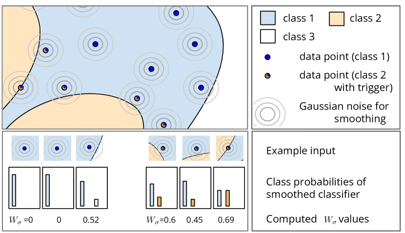
Figure 1: Differing local smoothness around points with and without trigger (top) and the computation of $W_{\sigma}$ (bottom) to distinguish them. The setting is inspired by the hypothesis that backdoored points (yellow with blue) live closer to their original class (yellow area) than benign test data (blue). Hence, the area around backdoors is not smooth. Benign test data instead live in a smooth environment. Our measure allows to distinguish these two cases. To compute our measure, we sample Gaussian noise around the test point (gray circles), and compute the class probabilities of the resulting approximated smoothed classifier (visualized as histograms). We then compute the entropy of the class probabilities and depict them below the probability distribution. $W_{\sigma}$, or the resulting values reflect the difference in smoothness between the two cases.

Intuition

Our goal is to measure the smoothness around data with and without an active trigger. We present an intuition in Figure 1, where backdoored data (yellow dots with blue) live close their original class (yellow) in a non-smooth area. Clean test data (blue dots), instead, live in a smooth area. Our measure approximates a smooth classifier by sampling Gaussian noise around the test point (gray circles). We then compute the distribution over the output classes and derive a measure that describes the smoothness of this output distribution, as visible at the bottom of Figure 1. If for example only one class is outputted across the sampled ball, the measure is zero. Our measure, $W$, when computed on a batch of points, yields insights about the smoothness of the area the input data lives in.

Notation

Let us assume that we are given an input sample $\boldsymbol{x}\in\mathcal{X}\subseteq\mathbb{R}^{d}$ of $d$ dimensions to be classified as one of the $c$ classes $\{1,\ldots,c\}$. The classification function is represented as $g_{k}:\mathcal{X}\mapsto\mathbb{R}$, providing a continuous-valued confidence score for each class $k=1,\ldots,c$. The classifier will assign the input sample $\boldsymbol{x}$ to the class $k$ exhibiting the highest classification confidence, i.e., $k=\operatornamewithlimits{\arg\,\max}_{j=1,\ldots,c}g_{j}(\boldsymbol{x})$. We can thus define $f_{k}$ as the one-hot encoding of the predicted class labels as:

$$f_{k}(\boldsymbol{x})=\left\{\begin{array}[]{ll}1\,,&\mbox{if }k=\operatornamewithlimits{\arg\,\max}_{j=1,\ldots,c}g_{j}(\boldsymbol{x})\,,\\ 0\,,&\mbox{otherwise \,.}\end{array}\right.$$ (1)

Smoothing

Let $\boldsymbol{\delta}\sim\mathcal{N}(\boldsymbol{0},\sigma^{2}\mathbb{I})\in\mathbb{R}^{d}$, i.e., an isotropic Gaussian perturbation parameterized by its standard deviation $\sigma$. We denote the probability of classifying $\boldsymbol{x}+\boldsymbol{\delta}$ as class $k$ with

$$p_{k}(\boldsymbol{x})=\mathbb{E}_{\boldsymbol{\delta}\sim\mathcal{N}(\boldsymbol{0},\sigma^{2}\mathbb{I})}f_{k}(\boldsymbol{x}+\boldsymbol{\delta})\simeq\frac{1}{n}\sum_{i=1}^{n}f_{k}(\boldsymbol{x}+\boldsymbol{\delta}_{i})\,,$$ (2)

where each probability value $p_{k}(\boldsymbol{x})$ depends on the choice of $\sigma$ and the amount of sampled points $n$. Intuitively, the larger $n$, the more accurate are the approximated class probabilities $p_{k}(\boldsymbol{x})$. To understand the effect of $\sigma$, consider the third clean test point in Figure 1. If $\sigma$ is very small, the sampled ball is classified entirely as blue class. As $\sigma$ increases, the white class’ probability will be nonzero, too.

We are interested in the smoothness of the classification probabilities. As the entropy is zero if only one class has all the probability mass, and is maximal when $p_{1}(\boldsymbol{x})=p_{2}(\boldsymbol{x})=\dots=p_{c}(\boldsymbol{x})$, we define our measure $W$ as the entropy of the smoothed probability outputs,

$$W_{\sigma}(\boldsymbol{x})=-\sum_{k=1}^{c}p_{k}(\boldsymbol{x})\log{p_{k}(\boldsymbol{x})}\,.$$ (3)

We further write $W_{\sigma}$ to highlight the dependency of $W$ on $\sigma$, using the latter as subscript. To conclude, we would like to emphasize that as the measure is zero at the maximal smoothness, and maximal when the surface is very non-smooth, it actually quantifies the wobbliness of the decision surface. In reference to this wobbliness, we name the measure $W$.

$W$ is thus well suited to study backdoor smoothing: if the measure is low for a set of points, we can deduce that the local decision surface is very smooth around these points. We now turn to our empirical results when analysing backdoored neural networks using $W_{\sigma}$.

3 Empirical Evaluation

We first evaluate in Section 3.1 $W_{\sigma}$’s parameters and their influence on the measurement. Afterwards, in Section 3.2, we study backdoors though the lens of $W_{\sigma}$.

3.1 Parameters of $W$

Before investigating backdoor attacks using $W_{\sigma}$, we empirically validate our understanding of its parameters to motivate our choices of these parameters later on. As stated in Section 2, $W_{\sigma}$ relies on two important parameters. This includes the variance of the noise distribution $\sigma$ which influences how local the smoothed classifier is. Further, the amount of sampled noise points $n$ per test point influences $W_{\sigma}$. We show that as $n$ is larger, the measure is more stable. Yet, an $n$ as small as $250$ points suffices to obtain a stable output of the measure. We first outline the experimental setting and the layout of the plots, before we turn to the parameters $\sigma$ and $n$. Afterwards, we proceed with our study on backdoors.

Experimental Setting

We study two datasets, Fashion MNIST [46] and CIFAR10 [23]. On the former, we deploy small networks which achieve an accuracy of around $88$%. These networks contain a convolution layer with $32$ $3\!\times\!3$ filters, a max-pooling layer of $2\!\times\!2$, another convolution layer with $12$ $3\!\times\!3$ filter, a dense layer with $50$ neurons, and a softmax layer with $10$ neurons. We further experiment on CIFAR10, where we train a ResNet18 [19] $200$ epochs to achieve an accuracy of $91.8$%. In general, we report the results of one network in this subsection, yet rerun the experiments several times to confirm that the results remain consistent.

Plots

Given a batch $X$ of size 250 test points, we plot the distribution of $W_{\sigma}(X)$ using box plots. These plots depict the mean (orange line), the quartiles (blue boxes, whiskers) and outliers (dots). We follow a standard definition for outliers by [14]: An outlier is defined as a point further away than 1.5 the interquartile range from the quartiles. More concretely, $Q_{25}$ is the first quartile and $Q_{75}$ is the third quartile (and $Q_{50}$ is the median). Value $\nu$ is an outlier if and only if

$$\nu>Q_{75}+1.5\times(Q_{75}-Q_{25})\text{ or }\nu<Q_{25}-1.5\times(Q_{75}-Q_{25})\text{ ,}$$ (4)

in other words if $\nu$ is more than $1.5$ times the interquartile range $(Q_{25}-Q_{75})$ away from either quartile $Q_{25}$ or $Q_{75}$.

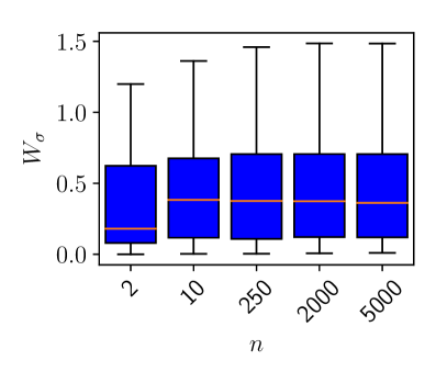
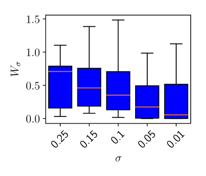
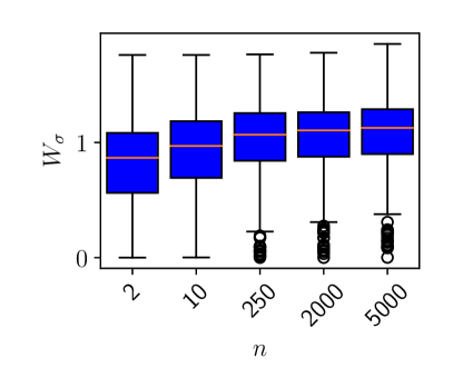
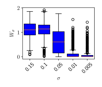
Figure 2: Box-plots reporting $W_{\sigma}$ values on clean samples from Fashion MNIST (top row) and CIFAR10 (bottom row), as a function of the number of noised points $n$ (left) and $\sigma$ (right).

Parameters $\mathbf{\sigma}$ and $\mathbf{n}$

Both parameters are visualized in Figure 2. We first describe the effect of $n$, the number of sampled points around each given test point. Independent of the dataset used, as $n$ increases, the mean of the computed $W_{\sigma}$ values increases and the spread decreases. Starting from roughly 250 sampled points, the results are relatively stable, and the changes in mean and spread are rather small. We conclude that a rather small number of sampled points around each test point, e.g. $250$, is sufficient to approximate the classifier for our measure.

We verify our intuition about $\sigma$. As our features are in range $[0,1]$, we also choose $\sigma\in[0,1]$, where we do not truncate the noise points if they are outside $[0,1]$ after adding the noise. As CIFAR10 has a larger features space due to the images being colored, we plot the results for smaller values of $\sigma$ in this case. Independent of the dataset, as the $\sigma$ decreases, the spread of the mean of $W_{\sigma}$ values decreases, until there is no more variance at $\sigma=0.01$. This is expected, as we sample a smaller and smaller radius. Yet, the transition is smoother on Fashion MNIST than on CIFAR10. On the latter, the results for $\sigma=0.15$, $\sigma=0.1$, $\sigma=0.01$ and $\sigma=0.005$ are similar.

Conclusion on Parameter Choice

When re-sampling each point in batch $X$ at least $250$ times, $W_{\sigma}(X)$ is sufficiently stable. Furthermore, $\sigma$ as a parameter allows us to measure the uncertainty of the smoothed classifier at a different granularity.

3.2 Backdoor Smoothing

We are now equipped with an understanding of $W_{\sigma}$ that allows us to study backdoor smoothing. In Section 3.2.1, we first describe the experimental setting of the following experiments. Afterwards, in Section 3.2.2, we show that backdoor smoothing, or $W_{\sigma}$ changes between a backdoor and clean test data. In Section 3.2.3, we deepen this understanding and correlate backdoor success with $W_{\sigma}$ and backdoor smoothing. Finally, in Section 3.2.4, we investigate whether backdoors are a necessary condition for backdoor smoothing. In other words, we first verify that backdoors cause backdoor smoothing and then test whether other patterns induce backdoor smoothing as well.

3.2.1 Experimental Setting

However, we first detail the threat model and experimental setup before we describe the results of our qualitative study.

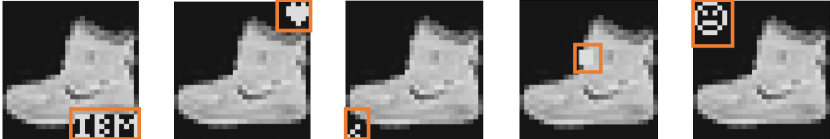
Figure 3: Possible backdoors on Fashion MNIST.

Attacker and Threat Model

A range of threat models have been studied in the literature, depending on whether the victim uses a pre-trained model or trains the model himself. Furthermore, the attacker can target one or several classes with the inserted backdoor. In other words, both the percentages of backdoor points in training as well as the number of targeted classes may vary. To avoid that any of these factors influences backdoor smoothing, we capture each of the previously mentioned factors in the following three threat models:

1. The victim is unable to inspect the training data, as they receives only the pre-trained model. The attacker is thus able to poison a large fraction of the training data and targets one class, as done in the work by [43] and [7]. We poison 15% of the training data, choose one target class and add the trigger to all classes except the target class.

2. This is a variation of the first threat model and was introduced by [17]. As before, we poison 15% of the training data, but the backdoor is added to each class. The output is now determined as the previous class $c+1$ modulo the number of classes.

3. The attacker alters the training data, because the victim trains the model themselve. As the victim might inspect the data before training the model, the amount of injected poisons is small (roughly 250 for more than 50,000 training points) as done by [41] and [7].

In all cases, a backdoor pattern is added to a portion of the training samples. Examples of such a pattern on image classification tasks are shown in Figure 3. Many of these backdoors are also used by [7] and [17]. We draw a backdoor pattern from this set, and overwrite the original pixels in the lower right corner with the corresponding trigger.

Model and Datasets

We train a small convolutional neural network on Fashion MNIST that is able to learn the backdoors well: a convolution layer ($64$ $3\!\times\!3$ filters), a max-pooling layer ($2\!\times\!2$), another convolution layer ($32$ $3\!\times\!3$ filters), two dense layers with $500$ neurons are followed by a softmax layer with $10$ neurons. To reduce the impact of randomness, we train and repeat the experiments multiple times. The trained models achieve around $90$% accuracy on benign data, and $99$% on inputs with the backdoors. On the CIFAR10 data, we use a ResNet18 architecture. As the smoothness of the classifier might be affected by overfitting, and we assume the small classifier above to overfit, we train the CIFAR networks few epochs to underfit the benign data at around $60$% accuracy. The CIFAR networks however perform in general well, or with accuracy of $>99$%, on test points with an active trigger.

$W_{\sigma}$ Parameters

As we have seen in Section 3.1, $W_{\sigma}$ is sufficiently stable we re-sample each input point $250$ time or more often. We hence set $n=250$ unless otherwise mentioned. More challenging is the choice of a suitable $\sigma$, which we will tackle in our first experiment in the next subsection.

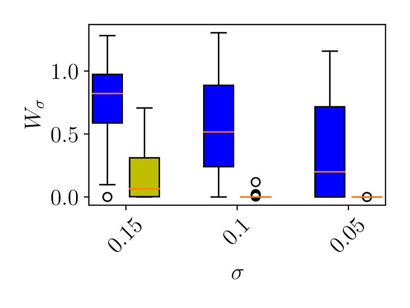
(a) Functional trigger

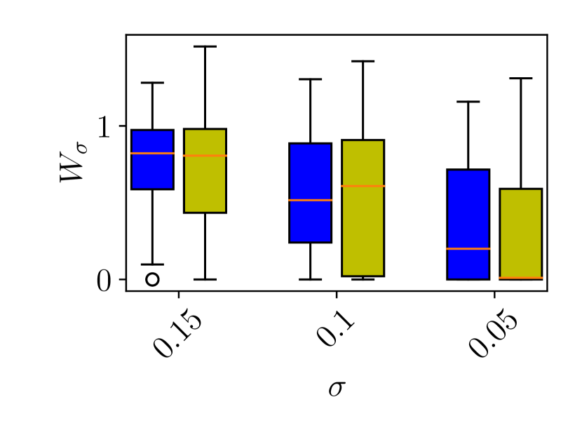
(b) Benign data

Figure 4: $W_{\sigma}$ and backdoors on Fashion MNIST. We compare clean test data (blue) and a functional trigger (99% accuracy, left plot)/an unused trigger (9% accuracy on poisoning labels, 89% on clean labels, right plot).

3.2.2 Effect of Backdoors on the Decision Surface

Before we deepen our understanding on the correlation between $W_{\sigma}$ and backdoor accuracy and which samples induce backdoor smoothing, we first need to understand at which locality differences arise. We thus first show the characteristics of samples around a backdoor and how $W_{\sigma}$ can capture them at different localities, depending on the parameter $\sigma$.

Experimental Setting

We consider two batches with 25 randomly chosen test points. The first batch $X_{C}$ contains clean test data, the second, $X_{A}$, contains test data with an active trigger the network was trained on. The trigger is the leftmost pattern from Figure 3, and used in training as specified in threat model T1. We plot the distributions of $W_{\sigma}(X_{C})$ (blue) and $W_{\sigma}(X_{A})$ (yellow) using the box-plots from the previous experiments in Figure 4 on the left. As a sanity check, we repeat the experiments using an additional batch $X_{NA}$ where we add the fourth pattern from Figure 3 as an inactive trigger. In other words, the network has not been trained on this trigger pattern. We draw a new batch $X_{C}$ and plot $W_{\sigma}(X_{C})$ (blue) and $W_{\sigma}(X_{NA})$ (yellow) on the right in Figure 4.

Results

We find that the local uncertainty of the smoothed classifier, measured by $W_{\sigma}$, is largely different for data with and without the active trigger pattern. On data with no trigger or an inactive trigger, $W_{\sigma}$ indicates that the decision surface is not very smooth. On the other hand, and in particular at small $\sigma$, the distribution of $W_{\sigma}$ shows that the smoothed classifier is very certain on the data with the active trigger.

Conclusion

Using our measure $W_{\sigma}$, we found that the classification output remains consistent regardless of the noise added to compute $W_{\sigma}$, and the decision surface around the sample with an active trigger is very smooth. This behavior is the attacker’s goal: as soon as the backdoor is present, other features become irrelevant. We call this property backdoor smoothing.

Kendall’s $\tau$: $-0.5$, $p=0.001$               Kendall’s $\tau$: $-0.49$, $p=1.5e^{-10}$
Pearson corr.: $-0.77$, $p=7.5e^{-5}$            Pearson corr.: $-0.58$, $p=1.8e^{-8}$

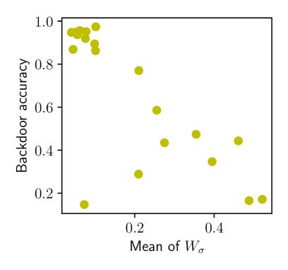
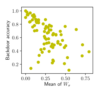
Figure 5: Backdoor accuracy and average $W_{\sigma}$ on CIFAR10 for threat model T1 (left) and Fashion MMIST for T1 (right). Above the plots, we write the computed p-values for Kendall’s $\tau$ and Pearson correlation, two tests with H₀ that no correlation is present.

3.2.3 Backdoor Accuracy and $W_{\sigma}$

In the previous experiments, we provided first evidence of backdoor smoothing, highlighting that the decision surface is smoother around backdoored samples. As hypothesized, this implies that the classifier ignores the noise added to compute $W_{\sigma}$. One interpretation is that this is a necessary condition, i.e., a low value of $W_{\sigma}$ implies that a trigger was learned well by the network. We now further validate this hypothesis.

Experimental Setting T1

To this end, we study T1 and train Resnets on CIFAR10. This time, we train 12 networks on the third backdoor trigger and 12 on the fifth backdoor trigger shown in Figure 3, using threat model T1. As before, we exclude backdoors with accuracy below random guess. As before, the smaller trigger seems harder to learn, with 4 networks not achieving random guess accuracy on the trigger. For the second trigger, all networks perform very well on the trigger.

Results T1

We plot the mean of $W_{\sigma}$ over a batch of triggered test points and the backdoor accuracy for each backdoor in the left plot in Figure 5. As before, backdoor accuracy and the mean of $W_{\sigma}$ seem negatively correlated. If the backdoor accuracy (y-axis) is very high, then the mean of $W_{\sigma}$ (x-axis) is low (left upper corner in the plot). Few points exhibit a backdoor accuracy below 0.4, these are spread far apart. As before, we validate correlation using Kendall’s $\tau$ and Pearson correlation. The correlation is quantified with -0.5 (Kendall’s $\tau$) and -0.77 (Pearson), and again negative. The p-values are $0.001$ (Kendall’s $\tau$) and $7.5e^{-5}$ (Pearson correlation), and thus confirm that backdoor accuracy and the mean of $W_{\sigma}$ are negatively correlated. Both p-values are larger than in the previous case, which is most likely due to the smaller sample size (17 cases here vs 79 cases in the experiments on Fashion MNIST).

Experimental Setting T2

We repeat the experiments with 5 networks on the third backdoor trigger, and 5 networks on the fifth backdoor trigger from Figure 3 on Fashion MNIST, using threat model T2. As we target each class, we take a batch of test points with active trigger for each class $c$, $X_{c}$, and compute $\mu(W_{\sigma}(X_{c}))$, e.g. the mean of $W_{\sigma}$ on the batch. We compute Backdoor accuracy separately for each class and exclude backdoors with an accuracy below random guess. For the small trigger, these are 19 out of 50 backdoor/target class pairs. For the larger smiley trigger, 2 are excluded. This reflects that the smaller trigger, as it has fewer features, is harder to learn for the networks.

Results T2

We visualize the results in the right plot in Figure 5. The accuracy and the mean of $W_{\sigma}$ seem negatively correlated. If the backdoor accuracy (y-axis) is very high, then the mean of $W_{\sigma}$ (x-axis) is low (left upper corner in the plot). As the mean of $W_{\sigma}$ values increases, the accuracy decreases and also varies more. To validate our intuition that both quantities are correlated, we compute Kendall’s $\tau$ [22] and Pearson correlation [34] on our sample. Both tests assume no correlation between the two features (backdoor accuracy and $W_{\sigma}$) as H₀. Both tests reject the H₀ with very small p-values of $1.5e^{-10}$ (Kendall’s $\tau$) and $1.8e^{-8}$ (Pearson correlation), confirming the correlation visible in the plots. The correlation is quantified with -0.49 (Kendall’s $\tau$) and -0.58 (Pearson), and is indeed negative.

Conclusion

We conclude that the mean of $W_{\sigma}$ over a batch of test points with an active trigger correlates negatively with backdoor accuracy. In other words, high local smoothness correlates positively with backdoor accuracy. This confirms our previous intuition that non-trigger features become more irrelevant when the accuracy on the trigger is higher. In other words, the results confirm that backdoor smoothing holds in general and is related to backdoor accuracy.

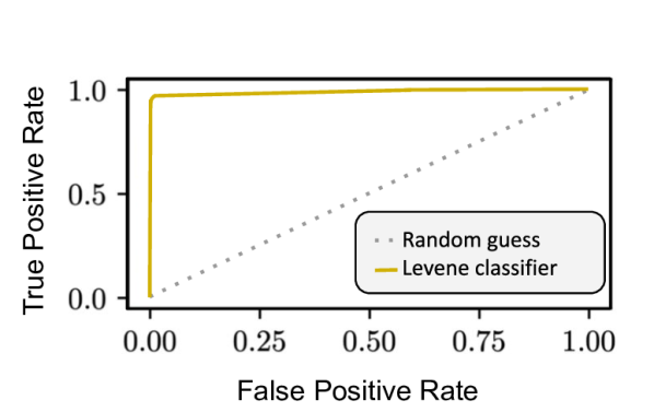
(a) CIFAR10, 15% poisons

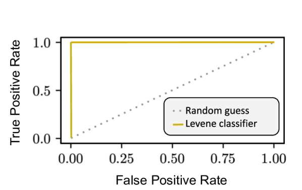
(b) Fashion MNIST, 250 poisons

Figure 6: ROC curve of a classifier based on $W_{\sigma}$ and the Levene test to detect differences between samples without and with active trigger (yellow) and corresponding random guess baseline (gray dots).

3.2.4 Smoothness-inducing Patterns

Given the differences in smoothness for benign test data and data with a trigger, the question remains whether this smoothness is unique and only caused by learned backdoors. In other words, we investigate whether backdoors are a necessary condition for backdoor smoothing. To this end, we test on a large scale whether $W_{\sigma}$ differs statistically when computed on batches of test data with and without functioning trigger. To assess that this difference is consistent (e.g., $W_{\sigma}$ is overall smaller when the trigger in the input batch is active), we build a classifier which we evaluate based on ground truth labels. To further confirm that backdoors are the only patterns to introduce backdoor smoothing, we also evaluate the test on universal adversarial examples [30] and unseen, crafted backdoor candidates [43].

Experimental Setting

We train 3 networks on clean data and 9 networks with different implanted backdoors. Of the latter backdoored networks, three are trained with backdoors one, three and four each from Figure 3. We study two settings: T1 on CIFAR10 using ResNets and T3 on Fashion MNIST. In each setting, $W_{\sigma}$ is computed on a batch of clean data for each network and on the active trigger for backdoored networks. To test for false positives, we also evaluate on backdoors not used in training. To this end, we also add all other five backdoors in Figure 3. We feed the output of $W_{\sigma}$ on the corresponding batches in a statistical test. As opposed to a single accuracy value, we opt to plot the discriminating power of the test as a receiver operating characteristic (ROC) curve. This ROC curve assesses in a more general manner how well the test separates the two classes, in our case backdoored and unbackdoored networks. More specifically, we use the ground truth knowledge from generating the data and pair active/inactive triggers with clean samples or clean with clean samples to evaluate the test.

Choice of Statistical Test

Given the results from Section 3.2.2, we decide to use a statistical test with the $H_{0}$ hypothesis that both populations have equal variance as our classifier. We decide to use the Levene test [33] as this test can be used with a small sample size to prevent detection of overly small differences in the variances [42]. Although the Levene test assumes a normal distribution, which is not the case here, the test is robust if the actual distribution deviates. The test is however sensitive to outliers, which we consequently remove. To this end, we use the definition from above by [14]. If all points have the same value, we do not remove any outliers.

Active Triggers and $W_{\sigma}$

We plot the ROC curves in Figure 6. For T1 on CIFAR10 the obtained area under ROC curve is $0.99$. In the case of T3 on Fashion MNIST the area under the ROC curve is $1.0$. Both values correspond to a perfect classifier between active backdoor triggers and untrained triggers. We thus conclude that, jointly with the observations from Section 3.2.2, backdoors indeed induce a smoother decision surface. We will now show, however, that also other patterns differ in terms of smoothness as measured by $W_{\sigma}$.

Universal Perturbations and $W_{\sigma}$

Universal adversarial examples are perturbations that are crafted after training and lead to misclassification when added to several data points [30]. They are thus similar in that they lead to misclassification of several data points, yet differ in that the network has not been trained on these patterns. We repeat the previous experimental setting, however using universal perturbations instead of backdoor triggers added to the data when computing $W_{\sigma}$. We then compute the Levene test, and compute the area under the ROC curve. Assuming that universal perturbations induce backdoor smoothing, we consider the two ground truth labels clean and universal perturbation.

We plot the ROC curves in Figure 7. As visible in the left sub-figure, the area under the ROC curve for T1 on CIFAR10 is 0.05, where we make the observation that the labels are flipped: whereas active backdoor triggers showed less variances than benign data, benign data shows less variance then universal perturbations on CIFAR10. Using T3 on Fashion MNIST, however, we obtain an area under the ROC curve of $0.56$, which is comparable to random guess. In other words, the test is not able to distinguish samples with universal adversarial examples from benign data based on $W_{\sigma}$. In other words, our results on universal perturbations are inconclusive. However, universal examples also differ from backdoor triggers in so far as they do not require all samples they are added to to be misclassified as the same class.

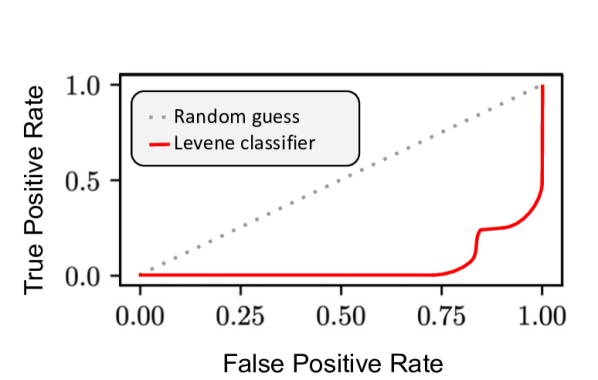
(a) CIFAR10, 15% poisons

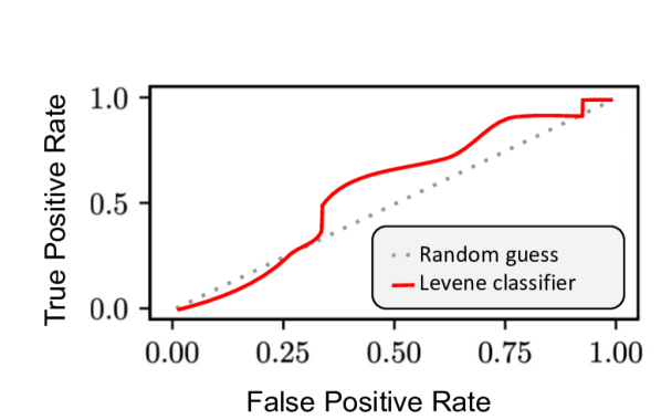
(b) Fashion MNIST, 250 poisons

Figure 7: ROC curve of a classifier based on $W_{\sigma}$ and the Levene test to detect differences between samples without and with universal perturbations (red) compared to a random guess baseline (gray dots).

Perturbations from Neural Cleanse

Yet, there are approach to craft a perturbation at test time with the constraint of outputting the same class for all samples. On example is Neural Cleanse Wang et al. [43], an approach to determine whether a network is backdoored by generating trigger candidates. The idea behind their algorithm is that a backdoor leads to a perturbation of minimal size that, when applied to any image (in a given input set), will cause all images to return the same fixed class. We generate a trigger candidate for each class on clean and backdoored models from our pool described above. As before, we add the candidates to clean test data, compute the $W_{\sigma}$, and feed the measure into the Levene test. The test detects all of the inputs with the crafted perturbation as backdoors with the same, very low p-value. As a sanity check, we add the patterns found to the training data (which has not been used to generate them) and find that the accuracy on the targeted class is 100% in all cases. The crafting mechanism was thus able to find a smoothness-inducing, although the patterns were not seen during training. We can thus refute that backdoors are a necessary condition for backdoor smoothing.

3.3 Summary of the Results and Discussion

In this section, we have investigated the local smoothness of networks trained with a backdoor trigger. At test time, our measure $W_{\sigma}$ indicates that the surface is smoother around a data point with the trigger than compared to a clean test point. We name this property backdoor smoothing. In particular, our experiments indicate that the smoother the local decision surface around the trigger, the higher is the accuracy of the trigger on the attacker’s chosen class. We further investigated whether an active backdoor trigger is a necessary condition for backdoor smoothing, and find this conjecture to be false. In other words, there exist other, smoothness-inducing patterns crafted after training that exhibit backdoor smoothing. These patterns induce smoothness although the network has never been exposed to these specific patterns during training. Our findings thus indicate that backdoor smoothing can be used to detect backdoors and also other, smoothing inducing adversarial perturbations. This entails patterns that are generated in the context of backdoor detection, raising the question of the implications of our work for backdoor mitigations. We will discuss these implications in the next section.

4 Implications for the Design of Mitigations

Backdoor smoothing has implications for the design of mitigations against backdoor attacks if they rely for example on smoothness assumptions to generate or verify a trigger.

Backdoor Smoothing and Trigger Generation

Some works explicitly use backdoor smoothing or analogous approaches to generate candidate triggers. For example [43] reverse engineer the trigger by collecting a batch of clean points and crafting a pattern that misclassifies all of them. Other approaches, like for example [44] or [45], craft a perturbation for each class pair, assuming the perturbation for the source and target backdoor class will be small if a trigger maps between the classes. Further [28] take advantage of a similar idea, yet assuming that individual neurons provide a stable output for a backdoor. We have shown that patters generated by these approaches might be in fact adversarial examples [11, 4, 39] that were not implanted into the training data. In this sense, the difference between a backdoor and another, smoothness-inducing pattern or adversarial example exhibiting backdoor smoothing is not necessarily clear.

Backdoor Smoothing and Trigger Verification

Analogous implications hold for approaches relying on smoothness to decide whether a pattern is a trigger or not. For example, [15] propose to perturb the input using superimposition of two images and then evaluate the consistency of the output classes. If one class prevails (e.g., the surface is smooth), the presence of a trigger is deduced. Analogously, [50] compute the variance of the logits between a clean image and an image with a universal adversarial perturbation [30] added. Here as well, the pattern is confirmed to be smoothness-inducing, and might be a backdoor or an adversarial example. In other words, there is no guarantee the found pattern was inserted with malicious intention into the training data.

Conclusion

When no ground truth information on a trigger pattern is available, the question whether a smoothness-inducing pattern was indeed implanted in the training data cannot be reliably answered. Some approaches tackle this issue by making additional assumptions on the trigger size [43] or incorporate more information like explanations and smoothness of the trigger pattern [18].

To finish the section, we would like to remark that there are conceptually unrelated defenses. To name a few examples, [48] compute a new model by interpolating in the loss space between two (potentially) backdoored models. Furthermore, defenses relying on pruning or retraining [27, 26, 1] are not related. These defenses have to be thoroughly evaluated depending on their own specifics.

5 Related Work

We first review related work in the area of backdoors. Afterwards, we describe randomized smoothing, a conceptually related technique to obtain robustness against perturbation at test time. To conclude, present input sensitivity measures, as some are also related to the smoothness of the classifier.

Backdoor Attacks

After the initial work on backdoor attacks [17, 8], many defenses were proposed [43, 28, 41, 7, 26]. Yet, no definite solution has been found, leading to an ongoing arms-race  [40, 31]. In contrast to many works in the area of backdoors or poisoning in general, we do neither propose a defense nor an attack. Instead, we study the phenomenon of backdoors in relation to local sensitivity. Along these lines, [13] show a trade-off in strength of the attack and detectability for general poisoning. Analogously, [9] show that learning a backdoor requires the model to globally increase complexity if the model’s complexity is not high enough. In contrast to both works, we study the local effect that backdoors have on a classifier. Furthermore, [3] study backdoor generalization using their formal framework in binary neural networks. They conclude that the trigger is only effective when combined with images from the training distribution. We have instead compared in distribution test data with and without trigger. Finally, [50] investigate the loss surface when generating a trigger and show that a GAN outperforms conventional, gradient based methods. Although gradients are correlated with local sensitivity, the authors focus on the problem of recovering the trigger from clean data, and do not investigate the gradients with respect to the type of data (e.g., with and without trigger).

Randomized Smoothing

Our measure is conceptually related to randomized smoothing, a certified defense against test-time attacks on models introduced by [10]. Analogous to $W_{\sigma}$, a smoothed classifier is approximated using Gaussian noise and its class probabilities are computed. However, the authors derive a bound on adversarial robustness to $\ell_{2}$ perturbations from the probabilities, expressed as a radius in which the prediction of the model does not change. In this area, the classifier is naturally smooth, yielding a strong connection to $W_{\sigma}$. Randomized smoothing has been extended beyond Gaussian noise to encompass other metrics such as Wasserstein [25] and specific network architectures, like for example graph neural networks [20]. Extending $W_{\sigma}$ along these lines is thus straight forward.

Measures of Input Sensitivity

A detailed overview about both empirical and theoretical measures of input sensitivity and overfitting is given by [21]. Some of these measures are conceptually close to $W_{\sigma}$. For example, [12] introduce a measure that is also based on measuring the output variation for a sample perturbed using Gaussian noise. Further, [32] propose a measure based on the norm of input/output Jacobian. Both measures, however, are formally connected to overfitting, and conceptually work in a setting where several classifiers are trained on differently perturbed training data. Finally, [38] also propose a perturbation based measure. They empirically show that their measure exhibits differences for training and test data, related to a specific test time perturbations. We, instead, focus on backdoor trigger in our analysis, and do not constrain the perturbation to the manifold of the network. We further aim to understand the differences of input sensitivity for different groups of data, namely with and without active trigger at test time.

6 Conclusion and Future Work

To tackle the lack of understanding in backdoor attacks in deep learning, we studied backdoors from the perspective of local smoothness of the decision function. To this end, we proposed a measure, $W$, that quantifies this local smoothness of the decision surface. Our experiments showed a phenomenon we call backdoor smoothing: the decision surface is smoother around points with an active backdoor trigger pattern than around benign training points. More concretely, the smoothness around data points with the trigger pattern correlates with the trigger’s accuracy. We further tested whether backdoors are a necessary condition for backdoor smoothing. To this end, we confirmed that active backdoor triggers are reliably living in smooth areas of the decision function. However, we were also able to craft smoothness-inducing patterns that were not previously inserted in the training data. These samples are adversarial examples, and defending them is of independent interest.

Our findings imply that $W$ might be used as a defense against backdoors and also test-time perturbations that induce smoothness. We leave an in-depth evaluation of this defense for future work. Furthermore, our work is currently limited to the area of computer vision. However, as work in randomized smoothing shows, an extension of $W$ to other domains is straight forward. We also did not investigate how the decision surface changes in terms of smoothness when additional defensive measures are applied. The results from these experiments would for example yield insights about how to combine different mitigations. Finally, our work does not encompass the design of an adaptive attacks against backdoor smoothing. We leave it for future work to answer the question whether such an attack is able to decouple backdoor smoothing and attack success, in particular without affecting clean accuracy.

References

- Aiken et al. [2021] Aiken, W., Kim, H., Woo, S., Ryoo, J., 2021. Neural network laundering: Removing black-box backdoor watermarks from deep neural networks. Computers & Security 106, 102277.
- Athalye et al. [2018] Athalye, A., Carlini, N., Wagner, D.A., 2018. Obfuscated gradients give a false sense of security: Circumventing defenses to adversarial examples, in: ICML, pp. 274–283.
- Baluta et al. [2019] Baluta, T., Shen, S., Shinde, S., Meel, K.S., Saxena, P., 2019. Quantitative verification of neural networks and its security applications, in: CCS.
- Biggio et al. [2013] Biggio, B., Corona, I., Maiorca, D., Nelson, B., Šrndić, N., Laskov, P., Giacinto, G., Roli, F., 2013. Evasion attacks against machine learning at test time, in: Machine Learning and Knowledge Discovery in Databases (ECML PKDD).
- Biggio et al. [2014] Biggio, B., Fumera, G., Roli, F., 2014. Security evaluation of pattern classifiers under attack. IEEE Transactions on Knowledge and Data Engineering 26, 984–996.
- Biggio and Roli [2018] Biggio, B., Roli, F., 2018. Wild patterns: Ten years after the rise of adversarial machine learning. Pattern Recognition 84, 317–331.
- Chen et al. [2019] Chen, B., Carvalho, W., Baracaldo, N., Ludwig, H., Edwards, B., Lee, T., Molloy, I., Srivastava, B., 2019. Detecting backdoor attacks on deep neural networks by activation clustering, in: Workshop on Artificial Intelligence Safety at AAAI.
- Chen et al. [2017] Chen, X., Liu, C., Li, B., Lu, K., Song, D., 2017. Targeted backdoor attacks on deep learning systems using data poisoning. arXiv preprint arXiv:1712.05526 .
- Cinà et al. [2021] Cinà, A.E., Grosse, K., Vascon, S., Demontis, A., Biggio, B., Roli, F., Pelillo, M., 2021. Backdoor learning curves: Explaining backdoor poisoning beyond influence functions. arXiv preprint arXiv:2106.07214 .
- Cohen et al. [2019] Cohen, J.M., Rosenfeld, E., Kolter, J.Z., 2019. Certified adversarial robustness via randomized smoothing, in: ICML.
- Dalvi et al. [2004] Dalvi, N., Domingos, P., Mausam, Sanghai, S., Verma, D., 2004. Adversarial classification, in: KDD, pp. 99–108.
- Forouzesh et al. [2021] Forouzesh, M., Salehi, F., Thiran, P., 2021. Generalization comparison of deep neural networks via output sensitivity, in: 2020 25th International Conference on Pattern Recognition (ICPR), IEEE. pp. 7411–7418.
- Frederickson et al. [2018] Frederickson, C., Moore, M., Dawson, G., Polikar, R., 2018. Attack strength vs. detectability dilemma in adversarial machine learning, in: 2018 International Joint Conference on Neural Networks (IJCNN), IEEE. pp. 1–8.
- Frigge et al. [1989] Frigge, M., Hoaglin, D.C., Iglewicz, B., 1989. Some implementations of the boxplot. The American Statistician 43, 50–54.
- Gao et al. [2019] Gao, Y., Xu, C., Wang, D., Chen, S., Ranasinghe, D.C., Nepal, S., 2019. Strip: A defence against trojan attacks on deep neural networks, in: Proceedings of the 35th Annual Computer Security Applications Conference, pp. 113–125.
- Gilmer et al. [2018] Gilmer, J., Adams, R.P., Goodfellow, I.J., Andersen, D., Dahl, G.E., 2018. Motivating the rules of the game for adversarial example research. CoRR abs/1807.06732.
- Gu et al. [2019] Gu, T., Liu, K., Dolan-Gavitt, B., Garg, S., 2019. Badnets: Evaluating backdooring attacks on deep neural networks. IEEE Access 7, 47230–47244.
- Guo et al. [2019] Guo, W., Wang, L., Xing, X., Du, M., Song, D., 2019. Tabor: A highly accurate approach to inspecting and restoring trojan backdoors in ai systems. arXiv preprint arXiv:1908.01763 .
- He et al. [2016] He, K., Zhang, X., Ren, S., Sun, J., 2016. Deep residual learning for image recognition, in: CVPR.
- Jia et al. [2020] Jia, J., Wang, B., Cao, X., Gong, N.Z., 2020. Certified robustness of community detection against adversarial structural perturbation via randomized smoothing, in: WWW.
- Jiang et al. [2020] Jiang, Y., Neyshabur, B., Mobahi, H., Krishnan, D., Bengio, S., 2020. Fantastic generalization measures and where to find them, in: ICLR.
- Kendall [1938] Kendall, M.G., 1938. A new measure of rank correlation. Biometrika 30, 81–93.
- Krizhevsky and Hinton [2009] Krizhevsky, A., Hinton, G., 2009. Learning multiple layers of features from tiny images. Technical Report. Citeseer.
- Lee et al. [2019] Lee, G.H., Yuan, Y., Chang, S., Jaakkola, T., 2019. Tight certificates of adversarial robustness for randomly smoothed classifiers, in: NeurIPS.
- Levine and Feizi [2020] Levine, A., Feizi, S., 2020. Wasserstein smoothing: Certified robustness against wasserstein adversarial attacks, in: International Conference on Artificial Intelligence and Statistics, pp. 3938–3947.
- Li et al. [2021] Li, Y., Koren, N., Lyu, L., Lyu, X., Li, B., Ma, X., 2021. Neural attention distillation: Erasing backdoor triggers from deep neural networks, in: ICLR.
- Liu et al. [2018a] Liu, K., Dolan-Gavitt, B., Garg, S., 2018a. Fine-pruning: Defending against backdooring attacks on deep neural networks, in: International Symposium on Research in Attacks, Intrusions, and Defenses, Springer. pp. 273–294.
- Liu et al. [2019] Liu, Y., Lee, W.C., Tao, G., Ma, S., Aafer, Y., Zhang, X., 2019. Abs: Scanning neural networks for back-doors by artificial brain stimulation, in: CCS.
- Liu et al. [2018b] Liu, Y., Ma, S., Aafer, Y., Lee, W., Zhai, J., Wang, W., Zhang, X., 2018b. Trojaning attack on neural networks, in: NDSS.
- Moosavi-Dezfooli et al. [2017] Moosavi-Dezfooli, S.M., Fawzi, A., Fawzi, O., Frossard, P., 2017. Universal adversarial perturbations, in: CVPR, pp. 1765–1773.
- Nguyen and Tran [2021] Nguyen, A., Tran, A., 2021. Wanet–imperceptible warping-based backdoor attack, in: ICLR.
- Novak et al. [2018] Novak, R., Bahri, Y., Abolafia, D.A., Pennington, J., Sohl-Dickstein, J., 2018. Sensitivity and generalization in neural networks: an empirical study, in: ICLR.
- Olkin [1960] Olkin, I., 1960. Contributions to probability and statistics: essays in honor of Harold Hotelling. Stanford University Press.
- Pearson [1895] Pearson, K., 1895. Notes on regression and inheritance in the case of two parents proceedings of the royal society of london, 58, 240-242.
- Rosenfeld et al. [2020] Rosenfeld, E., Winston, E., Ravikumar, P., Kolter, Z., 2020. Certified robustness to label-flipping attacks via randomized smoothing, in: International Conference on Machine Learning, PMLR. pp. 8230–8241.
- Salman et al. [2019] Salman, H., Li, J., Razenshteyn, I., Zhang, P., Zhang, H., Bubeck, S., Yang, G., 2019. Provably robust deep learning via adversarially trained smoothed classifiers, in: NeurIPS.
- Shafahi et al. [2018] Shafahi, A., Huang, W.R., Najibi, M., Suciu, O., Studer, C., Dumitras, T., Goldstein, T., 2018. Poison frogs! targeted clean-label poisoning attacks on neural networks, in: NeurIPS.
- Shu and Zhu [2019] Shu, H., Zhu, H., 2019. Sensitivity analysis of deep neural networks, in: AAAI.
- Szegedy et al. [2014] Szegedy, C., Zaremba, W., Sutskever, I., Bruna, J., Erhan, D., Goodfellow, I., Fergus, R., 2014. Intriguing properties of neural networks, in: Proceedings of the 2014 International Conference on Learning Representations, Computational and Biological Learning Society.
- Tan and Shokri [2020] Tan, T.J.L., Shokri, R., 2020. Bypassing backdoor detection algorithms in deep learning, in: European Symposium of Security and Privacy.
- Tran et al. [2018] Tran, B., Li, J., Madry, A., 2018. Spectral signatures in backdoor attacks, in: NeurIPS.
- Uttley [2019] Uttley, J., 2019. Power analysis, sample size, and assessment of statistical assumptions—improving the evidential value of lighting research. Leukos .
- Wang et al. [2019] Wang, B., Yao, Y., Shan, S., Li, H., Viswanath, B., Zheng, H., Zhao, B.Y., 2019. Neural cleanse: Identifying and mitigating backdoor attacks in neural networks, in: IEEE Symposium on Security and Privacy.
- Xiang et al. [2020] Xiang, Z., Miller, D.J., Kesidis, G., 2020. Detection of backdoors in trained classifiers without access to the training set. IEEE Transactions on Neural Networks and Learning Systems .
- Xiang et al. [2021] Xiang, Z., Miller, D.J., Kesidis, G., 2021. Reverse engineering imperceptible backdoor attacks on deep neural networks for detection and training set cleansing. Computers & Security 106, 102280.
- Xiao et al. [2017] Xiao, H., Rasul, K., Vollgraf, R., 2017. Fashion-mnist: a novel image dataset for benchmarking machine learning algorithms. arXiv preprint arXiv:1708.07747 .
- Zhang et al. [2017] Zhang, C., Bengio, S., Hardt, M., Recht, B., Vinyals, O., 2017. Understanding deep learning requires rethinking generalization, in: ICLR.
- Zhao et al. [2020] Zhao, P., Chen, P.Y., Das, P., Ramamurthy, K.N., Lin, X., 2020. Bridging mode connectivity in loss landscapes and adversarial robustness, in: ICLR.
- Zhu et al. [2019] Zhu, C., Huang, W.R., Li, H., Taylor, G., Studer, C., Goldstein, T., 2019. Transferable clean-label poisoning attacks on deep neural nets, in: ICML.
- Zhu et al. [2020] Zhu, L., Ning, R., Wang, C., Xin, C., Wu, H., 2020. Gangsweep: Sweep out neural backdoors by gan, in: Proceedings of the 28th ACM International Conference on Multimedia, pp. 3173–3181.
- Zhu et al. [2021] Zhu, L., Ning, R., Xin, C., Wang, C., Wu, H., 2021. Clear: Clean-up sample-targeted backdoor in neural networks, in: Proceedings of the IEEE/CVF International Conference on Computer Vision, pp. 16453–16462.