Low-frequency divergence and quantum geometry of the bulk photovoltaic effect in topological semimetals

Abstract

We study the low-frequency properties of the bulk photovoltaic effect in topological semimetals. The bulk photovoltaic effect is a nonlinear optical effect that generates DC photocurrents under uniform irradiation, allowed by noncentrosymmetry. It is a promising mechanism for a terahertz photodetection based on topological semimetals. Here, we systematically investigate the low-frequency behavior of the second-order optical conductivity in point-node semimetals. Through symmetry and power-counting analysis, we show that Dirac and Weyl points with tilted cones show the leading low-frequency divergence. In particular, we find new divergent behaviors of the conductivity of Dirac and Weyl points under circularly polarized light, where the conductivity scales as $\omega^{-2}$ and $\omega^{-1}$ near the gap-closing point in two and three dimensions, respectively. We provide a further perspective on the low-frequency bulk photovoltaic effect by revealing the complete quantum geometric meaning of the second-order optical conductivity tensor. The bulk photovoltaic effect has two origins, which are the transition of electron position and the transition of electron velocity during the optical excitation, and the resulting photocurrents are respectively called the shift current and the injection current. Based on an analysis of two-band models, we show that the injection current is controlled by the quantum metric and Berry curvature, whereas the shift current is governed by the Christoffel symbols near the gap-closing points in semimetals. Finally, for further demonstrations of our theory beyond simple two-band models, we perform first-principles calculations on the shift and injection photocurrent conductivities as well as geometric quantities of antiferromagnetic MnGeO₃ and ferromagnetic PrGeAl, respectively, as representatives of real magnetic Dirac and Weyl semimetals. Our calculations reveal gigantic peaks in many nonvanishing elements of photoconductivity tensors below photon energy $\sim$0.2 eV in both MnGeO₃ and PrGeAl. In particular, we show the $\omega^{-1}$ enhancement of the shift conductivity tensors due to the divergent behavior of the geometric quantities near the Dirac and Weyl points as well as slightly gapped topological nodes. Moreover, the low-frequency bulk photovoltaic effect is tunable by carrier doping and magnetization orientation rotation. Our work brings out new insights into the structure of nonlinear optical responses as well as for the design of semimetal-based terahertz photodetectors.

I Introduction

Topological semimetals are emerging as efficient infrared and terahertz photodetectors [1]. In contrast to semiconductors whose absorption spectum is bounded below by the band gap, semimetals can detect radiations down to the terahertz range because of their gapless spectrum. A promising mechanism for the generation of photocurrents in semimetals is the bulk photovoltaic effect. It refers to the generation of photocurrent under uniform irradiation of light due to the intrinsic inversion asymmetry of the system. Since the bulk photovoltaic effect does not require a bias voltage for breaking inversion symmetry, dark current noise can be suppressed [1].

To achieve high photosensitivity, we need to understand how to obtain large photoconductivity. It is believed that band topology plays an important role [2, 3, 4, 5, 6]. The bulk photovoltaic effect occurs due to the inversion-asymmetric transition of electron position or velocity during the optical excitation, and the resulting photocurrents are respectively called the shift current and the injection current [7]. In nonmagnetic systems, linearly polarized light induces shift currents while circularly polarized light induces injection currents. Remarkably, both the linear shift [4] and circular injection [5] currents were found to be intimately related to the topological quantities, the Berry connection and the Berry curvature, respectively. These discoveries have led to various theoretical and experimetnal studies searching for topological enhancement near the gap-closing points [8, 9, 10, 11, 12, 13, 14, 15, 16, 17, 18, 19].

However, while there is a concrete proportional quantitative relationship between the injection current and the Berry curvature, no such a quantitative relation exists between the shift current and the Berry connection. For example, a Dirac point in two dimensions has a quantized $\pi$ Berry phase, thus having a nontrivial Berry connection. Nevertheless, such a Dirac point does not generate a shift current because of its inversion symmetry. Furthermore, no simple quantitative relation was found between the shift current and the shift vector [20], a gauge-invariant quantity related to the Berry connection, without some special requirements like the momentum independence of the dipole matrix elements [21].

The bulk photovoltaic effect in magnetic topological semimetals is more poorly understood, although a recent work has revealed some general aspects [22]. Due to time-reversal symmetry breaking in magnetic systems, linearly (circularly) polarized light can generate injection (shift) currents as well as shift (injection) currents. There are some works highlighting the generation of large linear injection currents in magnetic systems [23, 24, 25, 26, 27, 22], but the relationship between the response and band topology has not been understood. Moreover, there has been very little attention to the circular shift current, while the first concept of the shift current appeared as a response to circularly polarized light [28, 29, 30]. One reason for this is that injection currents are typically stronger than the shift currents. Since there is a rapid progress in the experimental observation [31, 32, 33] and theoretical proposal [34, 35, 36, 37, 38, 39, 40, 41, 42] of various magnetic topological semimetals, addressing optical properties in magnetic topological semimetals is now a timely subject.

Response	Linear Injection	Circular Injection	Linear Shift	Circular Shift
Parity under $T$	$-$	$+$	$+$	$-$
Parity under $PT$	$+$	$-$	$-$	$+$
Geometric quantities	Quantum metric	Berry curvature	Symplectic Christoffel symbols	Christoffel symbols of the first kind
Leading divergence	$O(\tau\omega^{d-3})$		$O(\omega^{d-4})$

Table 1: Low-frequency properties of second-order DC photovoltaic responses. Linear and circular indicates the polarization of light. Injection and shift conductivities are defined by Eq. (II). The sign $\pm$ indicates the parity of the conductivity tensor under the action of time reversal $T$ and spacetime inversion $PT$. See Eqs. (III.1) and (III.1). In $T$- ($PT$-) symmetric systems, only the responses with the positive $T$- ($PT$-) parity appears. All of the four responses can appear when $T$ and $PT$ symmetries are both broken. Based on their symmetry properties, we call the linear injection and circular shift current responses as $PT$-symmetric responses and the linear shift and circular injection current responses as $T$-symmetric responses. Symplectic Christoffel symbols indicate the symplectic analog of the Christoffel symbol of the first kind (See Eq. (IV.2)). Here we consider only interband-transitive processes in the clean limit where the relaxation rate $\Gamma=\tau^{-1}$ is smaller than the photon frequency $\omega$. In this case, the injection current is typically larger than the shift current, and they become comparable when $\omega$ approaches $\Gamma$.

In this work, we reveal general low-frequency properties of the shift and injection currents in magnetic and nonmagnetic point-node semimetals. By employing symmetry and power-counting analysis, we determine the leading low-frequency divergence near the gap-closing point, as summarized in Table 1. We show that tilted Dirac and Weyl points can generate the leading divergence. While the bulk photovoltaic response in tilted Dirac and Weyl points have been studied [23, 24, 25, 13], here we approach them in a unified view and discover new aspects. Our theory covers type-I and type-II spectrum of Dirac and Weyl points in any dimensions. In particular, our analysis include type-II Dirac points in two dimensions and type-I and type-II Dirac points in three dimensions, which are relevant to magnetic Dirac semimetals, whose shift and injection currents have not been previously studied. It is widely known that the protection of Dirac points against opening the gap requires inversion symmetry, which forbids the bulk photovoltaic response. That is true in nonmagnetic systems. However, in magnetic systems, symmetry under the combination of spatial inversion $P$ and time reversal $T$, which is $PT$ symmetry, is enough for the protection [40, 39, 41, 42], so inversion symmetry can be broken. Also, we study the largely overlooked circular shift current in Weyl and Dirac systems. The circular shift current grows fast as the photon frequency gets smaller, and it scales as $\omega^{-1}$ in three dimensions. This indicates that Dirac semimetals in three dimensions can show divergent photovoltaic responses like Weyl semimetals, although the Berry curvature is identically zero due to $PT$ symmetry. In two dimensions, it grows faster as $\omega^{-2}$.

We find that tilted Dirac and Weyl points show what we call the separation of responses, where photocurrents of different origins manifest through different current directions. For example, circular shift and circular injection currents flow in different directions. This can be useful in the detection of shift currents in the coexistence of the stronger injection currents. The separation of responses can occur from the symmetry transformation property under magnetic operations $MT$ or $C_{2}T$, where $M$ and $C_{2}$ are mirror and twofold rotation, so it remains robust in the system beyond the ${\bf k}$-linear approximation as long as those symmetries are preserved.

Our symmetry and power-counting analysis are enough for understanding the general pattern of the response for systems with a linear spectrum. However, for a deeper understanding of the response, we propose a new perspective on the low-frequency bulk photovoltaic effect. We uncover the full geometric nature of shift and injection currents. Here, as well as the Berry curvature, another geometric quantity called the quantum metric has a crucial role. Since geometry has more information than topology about quantum states, we observe the consequence of band topology in a more broad perspective through geometric quantities. We show that the linear injection conductivity is determined only by the quantum metric near the gap closing, in the same way as the circular injection conductivity is determined by the Berry curvature. This completes the geometric understanding of the injection currents at the low-frequency regime. Furthermore, we show that the shift conductivities are related to a more interesting quantity, which is the Christoffel symbols. Unlike the Berry connection, which has a complicated relationship to the magnitude of the shift current, the Christoffel symbols directly control the magnitude of the response. In this viewpoint, the enhancement of the shift and injection current responses near the gap-closing point can be attributed to the divergence of the geometric quantities at the geometric singularity, i.e., the gap-closing point. Furthermore, our unique perspective allows to view the bulk photovoltaic effect as novel tools for experimental measurements of quantum geometry in materials.

Our geometric interpretation of the bulk photovoltaic effect is clearly distinguished from the one in Ref. [22], which also discuss the role of the quantum metric. In Ref. [22], the shift current is decomposed into four parts, and one of them was interpreted as the geometric contribution. The injection current is identified to have no geometric origin. These are in contrast to our interpretation in which both shift and injection currents are fully geometric responses. Only through our direct quantitative relationships the bulk photovoltaic effect can be identified as a useful measure of quantum geometry in experiments as well as a way to theoretically understand the low-frequency divergent behavior.

Finally, for further demonstrations of our theory beyond simple two-band models, we perform first-principles relativistic band theoretical calculations of the shift and injection photocurrent conductivities as well as geometric quantities in antiferromagnetic (AF) MnGeO₃ and ferromagnetic (FM) PrGeAl (as will be reported in Sec. VI below), respectively, as representatives of real magnetic Dirac and Weyl semimetals. In AF MnGeO₃, although both $T$ and $P$ symmetries are broken, the combined $PT$ symmetry is preserved [42]. Thus, AF MnGeO₃ was recently predicted to a rare magnetic Dirac semimetal. [42] As our theory predicts (Table I), we find nonzero elements of circular shift and linear injection photoconductivity tensors in AF MnGeO₃. In fact, several nonzero elements exhibit huge peaks below photon energy of $\sim$0.2 eV. Our calculations reveal that at least there are three Dirac points in the vicinity of the Fermi level and two of the Dirac points are accompanied by a slightly gapped Dirac point each. The calculated quantum metric and Christoffel symbol of first kind exhibit divergent behaviors near both the gapless and gapped Dirac points, thus leading to the geometric enhancement in linear injection and circular shift currents, respectively. In contrast, both $T$ and $PT$ symmetries are broken in FM PrGeAl [43], and hence all four types of the bulk photovoltaic effect may emerge in FM PrGeAl, as our theory predicts (Table I). Indeed, we find that many nonzero elements of all shift and injection conductivity tensors show gigantic peaks in the low-frequency range up to 0.1 eV. There are at least 160 type I and type II Weyl points within $\pm$0.1 eV of the Fermi level in FM PrGeAl [43]. Our calculations indicate that the low-frequency peaks can be further increased by up to a factor of 5 by raising the chemical potential from the Fermi level to the energy of certain Weyl points. Our calculations also reveal the divergent behaviors of both quantum geometric tensor and quantum geometric connection (symplectic Christoffel symbol and Christoffel symbol of first kind) near the Weyl points and also anticrossing topological nodes, thus leading to the gigantic low-frequency shift and injection currents in FM PrGeAl. Furthermore, we notice that FM PrGeAl is a soft ferromagnet [44]. Thus, the magnetization direction can be easily rotated away from the easy $c$-axis to, e.g., $a$-axis, and this may cause a topology change of the Weyl point distribution in the Brilloin zone [43], thereby resulting in significant changes in the shift and injection photoconductivities. Also, since the circular shift and injection conductivity tensors are antisymmetric with respect to the magnetization direction, they would change sign when the magnetization direction is reversed. All these observations show that the gigantic low-frequency shift and injection photocurrents in FM PrGeAl can be tuned by either carrier doping or magnetization direction rotation.

The outline of this paper is as follows. We explain the shift and injection currents as a second-order optical response in Sec. II. Then, we study the symmetry and low-frequency divergence of the shift and injection currents in Sec. III. Section IV enriches our analysis by revealing the quantum geometrical nature of the low-frequency responses. We elaborate more on the symmetry and divergence with concrete models and numerical calculations in Sec. V. In Sec. VI, we present our first-principles calculations on the shift and injection photocurrent conductivities as well as geometric quantities of AF MnGeO₃ and FM PrGeAl. In particular, we analyze the gigantic peaks in the calculated low-frequency photoconductivity spectra in MnGeO₃ and PrGeAl in terms of the divergent behaviors of the geometric quantities near the gapless and slightly gapped topological nodal points. Finally, we discuss several issues about the low-frequency divergence in Sec. VII.

II Shift and Injection currents

Let us expand current density $j$ in increasing power of the electric field $E$ as

$$j^{c} =\sigma^{c;a}_{(1)}E_{a}+\sigma^{c;ab}_{(2)}E_{a}E_{b}+\sigma^{c;abc}_{(3)}E_{a}E_{b}E_{c}+\ldots.$$ (1)

The first term is the familiar linear response, and the other terms are nonlinear responses. Since the current density oscillates in-phase with the electric field in the linear response, the DC photocurrent generation is inherently a nonlinear optical effect. In our work, we assume that the electric field is sufficiently small such that perturbation theory works (we discuss in Sec. VII how small it should be). While even-order responses to $E$ vanishes in centrosymmetric systems, they are allowed in noncentrosymmetric systems. The bulk photovoltaic effect studied in the present paper is thus primarily a second-order response.

The second-order optical response under the uniform illumination of light has the form $j^{c}(\omega_{1}+\omega_{2})=\sigma^{c;ab}(\omega_{1}+\omega_{2};\omega_{1},\omega_{2})E_{a}(\omega_{1})E_{b}(\omega_{2})$ in general. Let us focus on the DC (direct current) generation

$$j^{c}_{\rm DC} =\sigma^{c;ab}_{\rm DC}(\omega)E_{a}(\omega)E_{b}(-\omega),$$ (2)

where $j^{c}_{\rm DC}=j^{c}(0)$, and $\sigma^{c;ab}_{\rm DC}(\omega)=\sigma^{c;ab}(0;\omega,-\omega)$. In the clean limit — where the interband relaxation rate is smaller than the photon frequency and the band gap, interband transitions are described by two processes: shift and injection .

$$\sigma^{c;ab}_{\rm DC}=\sigma^{c;ab}_{\rm shift}+\sigma^{c;ab}_{\rm inj}.$$ (3)

The shift and injection currents correspond to the current generated by the change of the electron position and velocity, respectively, during the interband transition of electrons [7]. One can see this by noting that the shift and injection conductivities have the form of the Fermi Golden rule [7] (See Appendix C for explicit calculations). Explicitly, they have the form [46, 47]

$$\sigma^{c;ab}_{\rm shift} =-\frac{\pi e^{3}}{\hbar^{2}}\int_{\bf k}\sum_{n,m}f^{\rm FD}_{nm}(R^{c,a}_{mn}-R^{c,b}_{nm})r^{b}_{nm}r^{a}_{mn}\delta(\omega_{mn}-\omega)$$

$$\sigma^{c;ab}_{\rm inj} =-\tau\frac{2\pi e^{3}}{\hbar^{2}}\int_{\bf k}\sum_{n,m}f^{\rm FD}_{nm}\Delta^{c}_{mn}r^{b}_{nm}r^{a}_{mn}\delta(\omega_{mn}-\omega),$$ (4)

where $\int_{\bf k}=\int d^{d}k/(2\pi)^{d}$, $f^{\rm FD}_{n}$ is the Fermi-Dirac distribution of the band $n$, $f^{\rm FD}_{nm}=f^{\rm FD}_{n}-f^{\rm FD}_{m}$, $\hbar\omega_{mn}=\hbar\omega_{m}-\hbar\omega_{n}$ is the energy difference between bands $m$ and $n$, $H|n\rangle=\hbar\omega_{n}|n\rangle$, $r^{a}_{mn}=\braket{m}{i\partial_{a}}{n}$ and $v^{c}_{mn}=\hbar^{-1}\braket{m}{\partial_{c}H}{n}$, and we use the notation $\partial_{a}=\partial/\partial k_{a}$. $R^{c;a}_{mn}=r^{c}_{mm}-r^{c}_{nn}+i\partial_{c}\log r^{a}_{mn}$ is called the shift vector — characterizing the interband-transition of the displacement, and $\Delta^{c}_{mn}=v^{c}_{mm}-v^{c}_{nn}$ is the interband-transition of the velocity. $\tau$ is the relaxation time that saturates the injection current: withtout it, the injection of moving electrons and holes leads to a constant growth in time. We take the electron charge as $-e$ (i.e., $e>0$). Eq. (II) is valid with and without time-reversal symmetry.

III Symmetry and Power-Counting Analysis

To get a general perspective on the low-energy properties of the shift and injection currents, we review their symmetry properties and then study the pattern of low-frequency divergences. The key properties presented in this section are summarized in Table 1, and they serve as basic ingredients for the analysis in Sec. V.

III.1 Symmetry of the shift and injection conductivities

Let us first decompose the second-order DC conductivity into its real and imaginary parts:

$$\sigma^{c;ab}(\omega)=\sigma_{L}^{c;ab}(\omega)+i\sigma_{C}^{c;ab}(\omega).$$ (5)

Using $E^{*}(\omega)=E(-\omega)$ and Eq. (2), one can see that the conductivity can be symmetrized such that

$$\sigma_{L}^{c;ab}(\omega) =\sigma_{L}^{c;ba}(\omega),$$

$$\sigma_{C}^{c;ab}(\omega) =-\sigma_{C}^{c;ba}(\omega).$$ (6)

Therefore, we always consider conductivity tensors satisfying Eq. (III.1). We note that the expressions in Eq. (II) are already symmetrized. Assuming the form ${\bf E}(t)=|E|e^{-i\omega t}(\cos\phi,\sin\phi,0)+c.c.$ for linearly polarized light and ${\bf E}(t)=|E|e^{-i\omega t}(1,i,0)+c.c.$ for circularly polarized light, the real part of the second-order optical conductivity is

$${\rm Re}j^{c}_{\rm L-dc}=( \sigma^{c;xx}_{L}\cos^{2}\phi+\sigma^{c;yy}_{L}\sin^{2}\phi$$

$$+2\sigma^{c;xy}_{L}\sin\phi\cos\phi)|E^{2}|$$

$${\rm Re}j^{c}_{\rm C-dc}=( \sigma^{c;xx}_{L}+\sigma^{c;yy}_{L}-2\sigma^{c;xy}_{C})|E^{2}|.$$ (7)

The real part of the conductivity is responsible for the current generation regardless of the polarization,while the imaginary part of the conductivity is responsible for the current generated by the circularly polarized light. If one measures the current difference between the ones generated by left-circularly polarized light and right-circularly polarized light $\propto\sigma^{c;xy}-\sigma^{c;yx}$, only the imaginary part contributes. In the following, we call the real part $\sigma^{c;ab}_{L}$ as linear conductivity and the imaginary part $\sigma^{c;ab}_{C}$ as circular conductivity.

From the definition in Eq. (2) and the transformation properties of the current and electric field, it is clear that the second-order optical conductivity transforms like a third-rank tensor under spatial transformations. That is, $\sigma^{\prime c_{1};a_{1}b_{1}}_{\rm DC}={\cal M}_{c_{1}c}{\cal M}_{a_{1}a}{\cal M}_{b_{1}b}\sigma^{c;ab}_{\rm DC}$ under a point-group symmetry transformation $x_{a}\rightarrow x^{\prime}_{a}={\cal M}_{ab}x_{b}$ . However, one should be careful when taking time reversal for relaxational processes as is well-known from the Onsager reciprocity relations in linear response theory [48, 49, 50]. For example, it seems like Eq. (2) implies that time reversal reverses the sign of the DC conductivity for linearly polarized light. However, we need to additionally reverse the sign of phenomenological relaxation rate $\Gamma$, in order to make the decay in time to the growth in time. The correct time reversal for the second-order DC conductivity is

$$\sigma^{c;ab}_{\rm DC}(\omega,\Gamma)\rightarrow\sigma^{\prime c;ab}_{\rm DC}(\omega,\Gamma)=-\sigma^{c;ba}_{\rm DC}(\omega,-\Gamma).$$ (8)

See Appendix D. When applying this equality, the delta function and $\tau$ should be interpreted as $\pi^{-1}\Gamma/[(\omega_{mn}-\omega)^{2}+\Gamma^{2}]$ and $\Gamma^{-1}$, so they reverses sign under $\Gamma\rightarrow-\Gamma$. Thus, the real part of the shift and injection conductivity tensor transforms as

$$\sigma^{\prime c_{1};a_{1}b_{1}}_{\rm shift,L} ={\cal M}_{c_{1}c}{\cal M}_{a_{1}a}{\cal M}_{b_{1}b}\sigma^{c;ab}_{\rm shift,L}$$

$$\sigma^{\prime c_{1};a_{1}b_{1}}_{\rm inj,L} =(-1)^{s_{T}}{\cal M}_{c_{1}c}{\cal M}_{a_{1}a}{\cal M}_{b_{1}b}\sigma^{c;ab}_{\rm inj,L},$$ (9)

and the imaginary part transforms as

$$\sigma^{\prime c_{1};a_{1}b_{1}}_{\rm shift,C} =(-1)^{s_{T}}{\cal M}_{c_{1}c}{\cal M}_{a_{1}a}{\cal M}_{b_{1}b}\sigma^{c;ab}_{\rm shift,C}$$

$$\sigma^{\prime c_{1};a_{1}b_{1}}_{\rm inj,C} ={\cal M}_{c_{1}c}{\cal M}_{a_{1}a}{\cal M}_{b_{1}b}\sigma^{c;ab}_{\rm inj,C}.$$ (10)

under the spacetime symmetry transformation $(t,x_{a})\rightarrow(t^{\prime},x_{a}^{\prime})=((-1)^{s_{T}}t,{\cal M}_{ab}x_{b})$. Alternatively, one can verify these transformation rule by examining transformations of $R^{c,a}_{mn}$, $r^{a}_{nm}$, $\Delta^{c}_{mn}$ from the form in Eq. (II). See Appendix E for a derivation.

Knowing these symmetry transformation properties, one can use the MTENSOR [51] in the Bilbao Crystallographic Server to see which tensor components are required to vanish by symmetry for any of 80 magnetic point groups. For our purpose, the most important symmetries are simply time reversal $T$ and spacetime inversion $PT$ symmetries (note again that $P$ is always broken in the present paper). We summarize their role in Table. 1. While only linear shift and circular injection currents can be generated in time-reversal-symmetric systems, they vanish in $PT$-symmetric systems, so linear injection and circular shift currents can be generated. time-reversal symmetry and spacetime inversion symmetry are thus complementary to each other, as pointed out in [22]. This behavior is manifested in the geometric quantities related to the responses. As we show below in Sec. IV, $T$-symmetric responses are related to both of the Berry curvature and the quantum metric, while $PT$-symmetric responses are related to the quantum metric only. In general magnetic systems without $T$ and $PT$ symmetries, all of the four types of currents can be generated.

When there is $MT$ or $C_{2}T$ symmetry instead, where $M$ and $C_{2}$ are mirror and twofold rotation, a phenomenon of ”separation of responses” occurs, meaning that different directions manifest different types of responses. It is because those symmetries act like time reversal in some directions and act like spacetime inversion in the other directions. For example, $M_{x}T$ acts like time reversal in the $y$ and $z$ directions, whereas it acts as spacetime inversion in the $x$ direction. In this case, $x$-polarized light generates a shift current along $y$ and $z$ while generating an injection current along $x$. We demonstrate the separation of responses through model calculations in Sec. V and also through first-principles calculations in Sec. VI.

III.2 Power-counting analysis of the low-energy divergence

Let us now examine the low-energy divergence of the second-order responses in semimetals. We can estimate the divergence by counting the power of photon frequency in Eq. (II). Since the delta function has dimension $\omega^{-1}$, $R^{c}$ and $r^{a}_{mn}$ has dimension $k^{-1}$, and $\Delta^{c}$ has dimension $\omega/k$, the shift and injection conductivity scales as

$$\sigma^{c;ab}_{\rm shift}\sim\frac{e^{3}}{\hbar^{2}}\frac{1}{\omega}k^{d-3},$$

$$\sigma^{c;ab}_{\rm inj}\sim\frac{e^{3}}{\hbar^{2}}\tau k^{d-3}.$$ (11)

where $k$ is the characteristic wave vector. When the system has dispersion $E\propto k^{\alpha}$, $k\sim E^{1/\alpha}\sim\omega^{1/\alpha}$. Thus, smaller $\alpha$ is preferred to get large optical responses for small $\omega$ in 2D, while it is independent on the dispersion in 3D.

In lattice systems, stable Weyl points always (and also Dirac points protected by symmorphic symmetries [52]) appear pairwise according to the Nielsen-Ninomiya theorem [53, 54]. Therefore, a response in semimetals should be a sum of responses from different Weyl or Dirac points. However, different gap-closing points are located at different energy levels in general, so it is expected that only a particular point contributes to the low-energy response significantly [5]. An exact cancellation or reinforcement among different gap-closing points can occur due to symmetries, but it can be considered straightforwardly from the symmetry transformation properties of the conductivity tensor. In this regard, the response from a single gap-closing point can be associated with the low-energy response of a whole system.

Thus, we consider a gap-closing point with a linear dispersion, described by a Dirac Hamiltonian

$$H_{0}({\bf k})=\hbar v\sum_{a=1}^{d}k_{a}\Gamma_{a},$$ (12)

where $\Gamma_{a}$ are mutually anticommuting matrices, such that the spectrum has the form

$$E({\bf k})=\pm\hbar v|{\bf k}|.$$ (13)

In this case, we have

$$\sigma^{c;ab}_{\rm shift} \sim\frac{e^{3}}{\hbar^{2}}\frac{1}{\omega}\left(\frac{v}{\omega}\right)^{3-d},$$

$$\sigma^{c;ab}_{\rm inj} \sim\frac{e^{3}}{\hbar^{2}}\tau\left(\frac{v}{\omega}\right)^{3-d}$$ (14)

through a dimensional analysis. This divergence is expected to occur in the absence of a symmetry cancellation. However, Eq. (12) has too many symmetries, so we need to break them in general. A Dirac point has inversion symmetry (by definition it is nonchiral), so the second-order optical response is forbidden. Also, as noted in Ref. [25, 13, 22], a Weyl point described by Eq. (12) does not show a second-order optical response by linearly polarized light. It is because Eq. (12) has SO($d$) rotational symmetry in $d$ spatial dimensions. In 3D, the absence of mirror symmetry (chirality) in Weyl semimetals allows one unique nonvanishing independent component $\sigma^{3;12}_{{\rm inj},C}$ under circularly polarized light. Because a Weyl point in 3D has time-reversal symmetry around the gap-closing point, the circular shift current is also forbidden, and the generated DC current is the circular injection current. Even for a more general linear dispersion described by $H=\sum_{a,i=1}^{d}\hbar v_{ai}k_{a}\Gamma_{i}$, which has apparently less symmetry, only circular injection currents for a Weyl point can be nonvanishing. It is because the conductivity for this Hamiltonian is given by $\sigma^{c;ab}_{\rm DC}=v^{-3}v_{ai}v_{bj}v_{ck}\det(v_{ai}/v)\sigma^{k;ij}_{\rm DC,0}$ [13], where $\sigma^{k;ij}_{\rm DC,0}$ is the conductivity for $v_{ai}=v\delta_{ai}$, which is the case for Eq. (12) (See Appendix G for a derivation).

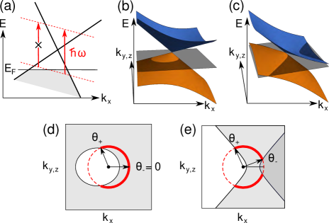
Figure 1: Optical excitation near a tilted Dirac or Weyl cone. (a) Excitation of electrons by the absortion of a photon with requency $\omega$. (b) Type-I spectrum. $|v^{\prime}/v|<1$. (c) Type-II spectrum. $|v^{\prime}/v|>1$. Here, $v$ is the velocity of a Dirac or Weyl fermion at zero tilting, and $v^{\prime}$ is the overall velocity shift by $\mu\rightarrow\mu+\hbar v^{\prime}k_{x}$, giving rise to a tilting of the cone. The gray planes in (b,c) show the Fermi level. (d,e) Optically active region in momentum space for (d) type-I and (e) type-II cases. Small black dots at the center indicates the location of the gap-closing point. Red circles around the point shows the surface satisfying $\hbar\omega=\hbar\omega_{c}-\hbar\omega_{v}=2\hbar vk$, where $k=0$ at the gap closing. Both conduction and valence bands are unoccupied in the white region, only the valence band is occupied in the light gray region, and both bands are occupied in the gray region. Electrons can be optically excited only on the solid red arcs (i.e., $\theta_{-}<\theta<\theta_{+}$, where $\theta$ is the absolute value of the polar angle in either 2D or 3D), which is in the light gray region.

The only way to generate the leading divergence for shift currents and linear injection currents is to tilt the Dirac or Weyl cone, as shown in Fig. 1. Since it allows anisotropic optical excitations around the gap-closing point, photocurrents can flow whose direction depends on the direction of the tilting. To see that other symmetry breaking gives subleading power in $\omega^{-1}$, let us add symmetry-breaking perturbations to the Dirac Hamiltonian.

$$H({\bf k})=H_{0}({\bf k})+\hbar\sum_{a}\sum_{p=0}^{\infty}\lambda_{p,a}k^{p}\Gamma_{a}.$$ (15)

Here, $\lambda_{p,a}$ is a constant parameter, $\Gamma_{a\neq 0}$ are mutually anticommuting matrices, and we also include $\Gamma_{0}$ as the identity matrix. Since the dimensionless parameter is $\lambda_{p,a}k^{p}\omega^{-1}\sim\lambda_{p,a}\omega^{p-1}$, responses due to perturbations in $\lambda_{p,a}$ have weaker low-frequency divergences for $p>1$. For example, let us consider a quadratic correction, resulting in the dispersion relation $E=\pm(\hbar vk+\lambda_{2}k^{2})$. Optical excitations occur in the region satisfying $\omega=E_{+}-E_{-}=2(\hbar vk+\lambda_{2}k^{2})$, i.e. $k=\omega/v(1-\lambda_{2}\omega/v^{2})+O(\omega^{3})$. By inserting this to Eq. (III.2), we have corrections to the leading divergence by a fraction $\left|(d-3)\lambda_{2}\omega/v^{2}\right|\ll 1$ for small $\omega$. At the $p=0$ order, $\lambda_{0,a}$ comes as either the chemical potential, the shift of the location of the gap-closing point, or a mass term , i.e., we can write the Hamiltonian as $H({\bf k})=-\mu+\sum_{a=1}^{d}(k-k_{0})_{a}\Gamma_{a}+M\sum\Gamma_{a>d}$. None of them generate nonvanishing shift and linear injection currents. $\mu$ breaks no symmetry, ${\bf k}-{\bf k}_{0}$ can be redefined as ${\bf k}$ such that gap closes at ${\bf k}=0$, and the mass term can serve as an inversion symmetry operator so that it forbids second-order optical responses. Let us now consider $p=1$. As we show above, the linear spectrum without tilting has zero shift and linear injection current responses. Thus, the remaining possibility is tilting the cone by adding $\lambda_{1,0}=-v^{\prime}\cos\theta$: this gives an overall tilting of energy levels by $\mu\rightarrow\mu+v^{\prime}k_{x}$.

Our analysis shows that the shift and injection conductivity tensors of tilted massless Dirac and Weyl points have the form

$$\sigma^{c;ab}_{\rm shift} =\frac{e^{3}}{\hbar^{2}}\frac{1}{\omega}\left(\frac{v}{\omega}\right)^{3-d}{\cal F}^{c;ab}_{\rm shift}\left(\frac{2\mu}{\hbar\omega},\frac{v^{\prime}}{v}\right),$$

$$\sigma^{c;ab}_{\rm inj} =\frac{e^{3}}{\hbar^{2}}\tau\left(\frac{v}{\omega}\right)^{3-d}{\cal F}^{c;ab}_{\rm inj}\left(\frac{2\mu}{\hbar\omega},\frac{v^{\prime}}{v}\right),$$ (16)

Let us explain how ${\cal F}$s depend on $v^{\prime}/v$ and $2\mu/\hbar\omega$ in general. When $\mu\neq 0$, i.e., when the Fermi level is away from the gap-closing point, the chemical potential sets the lowerbound for frequency, so ${\cal F}$s do not diverge as $\omega\rightarrow 0$.

When the Fermi level is exactly at the gap-closing point, i.e., $\mu=0$, ${\cal F}$s show significantly different behaviors for $|v^{\prime}/v|<1$ and $|v^{\prime}/v|>1$, which are called type-I and type-II [55], respectively [See Fig. 1(b,c)]. In the type-I case, tilting cannot generate shift and injection currents when $\mu=0$. It is because, in this case, the Fermi surface is a point, so anisotropic excitation cannot occur. Thus, only circular injection currents can be generated, which do not need tilting for its generation.

In contrast, in the type-II case, the Fermi surface has a finite size at $\mu=0$, so anisotropic excitation can occur in principle. However, it depends on whether the response is $T$-symmetric or $PT$-symmetric. While the $T$-symmetric responses (linear shift and circular injection) has a nontrivial response at $\mu=0$ [13], the $PT$-symmetric responses (linear injection and circular shift) has a vanishing response at $\mu=0$. This is related to the fact that a Hamiltonian with only ${\bf k}$-linear terms has an emergent $CPT$ symmetry, where $C$ is the particle-hole operator, and $CPT=1$: $(CPT)H({\bf k})(CPT)^{-1}=-H({\bf k})$. At $\mu=0$, $PT$-symmetric responses should be zero since they respect an effective $C$ symmetry also (where $(PT)^{-1}$ takes the role of an effective $C$ operator) — which reverses the direction of the current, while $T$-symmetric responses lack $C$ symmetry such that they can be nontrivial.

This shows that magnetic and nonmagnetic systems have the same low-frequency divergent behavior when $\mu=0$ exactly. Nevertheless, as far as $\mu$ is small but not exactly zero, we can still expect enhanced $PT$-symmetric responses at small frequency $\omega\sim 2\mu/\hbar$ by a factor in front of ${\cal F}$s in Eq. (III.2). Therefore, $PT$-symmetric responses in magnetic systems also can show a divergent behavior associated with the $\omega\rightarrow 0$ limit with a fixed ratio of $2\mu/\hbar\omega$.

We investigate the symmetry properties of the tilted Dirac and Weyl points more closely in Sec. V by explicitly calculating the conductivity tensors. Before that, we derive the general formula for the shift and injection conductivities for arbitrary Dirac Hamiltonians and provide their geometric aspects in the following sections. It adds more perspective on the transformation rule Eqs. (III.1) and (III.1) and the divergent behavior near the gap-closing point.

IV Quantum geometric aspects

In the previous section, we analyze the overall trend of shift and injection currents using symmetry and power-counting analysis. Here we show that every detail of the conductivity profile for the shift and injection currents is determined by quantum geometric quantities in the low-frequency regime. It was pointed out in Refs. [4, 6] that the shift current is related to quantum geometry because the shift vector includes the Berry connection — a geometric quantity. Following these works, the geometric nature of the shift and injection currents was previously discussed in several works [5, 22]. However, no simple quantitative relationship between the response and the geometric quantities has been found except for the circular injection conductivity [5]. In this section, we show that the shift and injection conductivities are proportional to geometric quantities that have natural geometric meaning on the Bloch sphere. These relationships are not limited to massless Dirac and Weyl points and are exact for any two-band system or $PT$-symmetric four-band system. It implies that interband-transitive photovoltaic responses at the low-frequency regime probe the quantum geometry of materials. In this perspective, the low-frequency divergence of the shift and injection current responses of gap-closing points can be attributed to their geometrically singular nature. Also, time reversal symmetry transformation of the conductivity tensors, which are quite confusing, can be simply understood from the transformation properties of the geometric quantities. In the following, we first derive the formula that relates injection and shift currents with the Bloch vector of general Dirac Hamiltonians with arbitrary matrix size in any spatial dimensions. Then, we provide a quantum geometric interpretation of our formula.

IV.1 Shift and injection conductivity for Dirac Hamiltonians

We consider the low-energy effective model systems described by the following $d_{M}\times d_{M}$ Dirac Hamiltonian

$$H({\bf k})=-\mu({\bf k})+\sum_{i}f_{i}({\bf k})\Gamma_{i},$$ (17)

where $\Gamma_{i}$ are mutually anticommuting matrices. This Hamiltonian described a single Dirac or Weyl point when $f_{i}({\bf k})=k_{i}$, but here we do not need to assume linear dispersion and consider general form of $f_{i}({\bf k})$s. In particular, the above Hamiltonian describes general two-band Hamiltonians when $d_{M}=2$, where $\Gamma_{i=1,2,3}$ are three Pauli matrices, and it describes general four-band $PT$-symmetric Hamiltonians (with $(PT)^{2}=-1$) when $d_{M}=4$, where $\Gamma_{i=1,\ldots,5}$ are five Gamma matrices.

Let us express the injection and shift conductivities in terms of $f_{i}$s. This makes theoretical analysis and numerical calculations convenient. As for the injection current, one can integrate the delta function easily by using $\Delta^{c}_{mn}=\partial_{c}\omega_{mn}$ such that $\Delta^{c}_{mn}\delta(\omega_{mn}-\omega)=\partial_{c}\Theta(\omega_{mn}-\omega)$. After that, we obtain

$$\sigma^{c;ab}_{\rm inj} =-\tau\frac{2\pi e^{3}}{\hbar^{2}}\int_{\omega_{cv}=\omega}\frac{d^{d-1}k}{(2\pi)^{d}}(\hat{n}\cdot\hat{c})Q_{ba}$$ (18)

for $\omega>0$, where $\hbar\omega_{cv}$ is the energy gap between the conduction and valence bands, $\hat{n}$ is the surface normal vector, and

$$Q_{ba} =\sum_{n\in\rm occ}\sum_{m\in\rm unocc}r^{b}_{nm}r^{a}_{mn}$$

$$=\sum_{i,j}\partial_{b}f_{i}\partial_{a}f_{j}\frac{d_{M}(\delta_{ij}-\hat{f}_{i}\hat{f}_{j}+iJ_{ij})}{8f^{2}}$$ (19)

is the so-called quantum geometric tensor [56] (See Appendix H for a derivation of the second equality). Here, $f=\sqrt{\sum_{i=1}f_{i}^{2}}$, and $J_{ij}=-i\sum_{k}\epsilon_{ijk}\hat{f}_{k}$ for $d_{M}=2$ and $J_{ij}=0$ for $d_{M}=4$. The vanishing of $J_{ij}$ for $d_{M}=4$ is due to the presence of $PT$ symmetry. $Q_{ba}$ is called the quantum geometric tensor because its real and imaginary parts are related to the quantum metric $g_{ba}$ and the Berry curvature $F_{ba}$ by

$$Q_{ba}=g_{ba}-\frac{i}{2}F_{ba}.$$ (20)

The relationship between the circular injection current and the Berry curvature was found in Ref. [5]. On the other hand, the role of the quantum metric in determining the linear injection current was not discussed in the literature. We explain more on the geometric meaning of the quantum geometric tensor in Sec. IV.2.

The shift current has more complicated form, and it can be related to the matrix elements of the derivatives of the Hamiltonian as [57]

$$R^{c,a}_{mn}r^{b}_{nm}r^{a}_{mn}=i\frac{v^{b}_{nm}}{\omega_{mn}^{2}}\left[w^{ac}_{mn}-\frac{v^{c}_{mn}\Delta^{a}_{mn}+v^{a}_{mn}\Delta^{c}_{mn}}{\omega_{mn}}\right]$$

$$+\frac{v^{b}_{nm}}{\omega^{2}_{mn}}\sum_{\omega_{p}\neq\omega_{m},\omega_{n}}\left(\frac{v^{c}_{mp}v^{a}_{pn}}{\omega_{mp}}-\frac{v^{a}_{mp}v^{c}_{pn}}{\omega_{pn}}\right),$$ (21)

where $w^{ac}_{mn}=\hbar^{-1}\braket{m}{\partial_{a}\partial_{c}H}{n}$ is the diamagnetic term. The second line involves virtual transitions among three different bands, so it vanishes in our Dirac system that has only two energy levels with energy $\hbar\omega_{c}=f_{0}+f$ and $\hbar\omega_{v}=f_{0}-f$, where $f=\sqrt{\sum_{i=1}f_{i}^{2}}$. It then follows that 

$$\sigma^{c;ab}_{\rm shift}(\omega) =-i\frac{2\pi e^{3}}{\hbar^{2}}\int_{\bf k}f^{\rm FD}_{vc}C_{bca}\delta(\omega_{cv}-\omega)$$ (22)

for $\omega>0$, where

$$C_{bca}=-i\sum_{n\in\rm occ}\sum_{m\in\rm unocc}R^{c,a}_{mn}r^{b}_{nm}r^{a}_{mn}$$

$$\qquad=\frac{d_{M}}{8f^{2}}\sum_{i,j}(\delta_{ij}-\hat{f}_{i}\hat{f}_{j}+iJ_{ij})\times$$

$$\bigg{[}\partial_{b}f^{i}\partial_{a}\partial_{c}f^{j}-\frac{1}{f}\left(\partial_{b}f^{i}\partial_{c}f^{j}\partial_{a}f+\partial_{b}f^{i}\partial_{a}f^{j}\partial_{c}f\right)\bigg{]}.$$ (23)

A special case of this formula was derived in Ref. [57] for two-band models with time-reversal symmetry. Our formula in Eq. (IV.1) extends the existing formula to describe arbitrary systems described by the Dirac Hamiltonian in Eq. (17). We show below that $C_{bca}$ has geometric meaning as a connection.

IV.2 Geometry on the generalized Bloch sphere

Let us explain the geometric meaning of the quantum geometric tensor $Q_{ba}$ as geometric quantities defined on the generalized Bloch sphere. This point of view is helpful for understanding the geometric meaning of $C_{bca}$ as well as that of $Q_{ba}$.

We consider the following general Dirac Hamiltonian in Eq. (17). Then, the generalized Bloch vector ${\bf f}({\bf k})$ is a map

$${\bf f}:{\rm BZ}\rightarrow{\mathbb{R}}^{d_{\Gamma}},$$ (24)

where $d_{\Gamma}$ is the number of Gamma matrices. This map defines a pull-back of the quantum geometric tensor from the ${\bf f}$-space to the Brillouin zone.

Let us recall that the quantum geometric tensor has the following form

$$Q_{ab} =\sum_{i,j}\partial_{a}f_{i}\partial_{b}f_{j}q_{ij},$$ (25)

where

$$q_{ij}=\frac{d_{M}(\delta_{ij}-\hat{f}_{i}\hat{f}_{j}+iJ_{ij})}{8f^{2}},$$ (26)

and $f=|{\bf f}|$. This is a pull-back of the quantum geometric tensor $q_{ij}$ defined in the ${\bf f}$-space to the momentum space by a transformation $\partial_{a}f_{i}$ of tangent vectors

$$\partial_{a}=(\partial_{a}f_{i})\partial_{i},$$ (27)

where $\partial_{i}=\partial/\partial f_{i}$. The quantum metric and the Berry curvature are given by

$$g_{ab} =\sum_{i,j}\partial_{a}f_{i}\partial_{b}f_{j}\eta_{ij},$$

$$\frac{1}{2}F_{ab} =\sum_{i,j}\partial_{a}f_{i}\partial_{b}f_{j}\epsilon_{ij},$$ (28)

where $\eta_{ij}$ and $\epsilon_{ij}$ are the real and imaginary parts of $q_{ij}$, i.e., $q_{ij}=\eta_{ij}-i\epsilon_{ij}$. In this viewpoint, the quantum metric and the Berry curvature are pull-backs of the metric $\eta_{ij}$ and the symplectic form $\epsilon_{ij}$ defined on the Bloch sphere. The metric $\eta_{ij}$ measures length $ds$ through $ds^{2}=\eta_{ij}df^{i}df^{j}$, and the symplectic form $\epsilon_{ij}$ measures the oriented area $dA$ through $dA=\epsilon_{ij}dx^{i}dx^{j}$ in the ${\bf f}$-space.

While the geometric quantity $\eta_{ij}$ is defined on the whole ${\bf f}$ space, it can be regarded to measure the length on the unit sphere with $f=1$, and it is irrelevant for the radial direction $f=|{\bf f}|$ . For example, $ds^{2}=(1/4)(d\theta^{2}+\sin^{2}\theta d\phi^{2})$ in polar coordinates when $d_{M}=2$. To see this without a coordinate transformation, first note that $P_{ij}=\delta_{ij}-\hat{f}_{i}\hat{f}_{j}$ is the projection to the plane perpendicular to $\hat{f}$. The metric measures the length only along the angular directions on a sphere with a fixed $f$. Also, the $f^{-2}$ factor normalizes the length such that only the angle between two points on a sphere is measured. Similarly, the symplectic form also measures the area on the unit sphere. In this sense, the quantum geometric tensor is a geometric quantity defined on the generalized Bloch sphere ($f=1$).

Another geometric quantity called the Levi-Civita connection also can be constructed on the generalized Bloch sphere. Its components are called the Christoffel symbols, and they can be written in two ways — the first and the second kind. The Christoffel symbols of the second kind $\gamma^{k}_{ij}$ are defined by

$$\partial_{i}{\bf e}_{j}=\sum_{k}\gamma^{k}_{ij}{\bf e}_{k},$$ (29)

where ${\bf e}_{i}$ is the projection of the unit vector along the $f_{i}$ direction to the tangent space by $P_{ij}=\delta_{ij}-\hat{f}_{i}\hat{f}_{j}$. It measures how vectors and tensors are changed as we move them parallel to the direction of the curved surface (which is the generalized Bloch sphere in our case) . We have

$$\gamma^{k}_{ij} =-\frac{f_{i}}{f^{2}}(\delta_{jk}-\hat{f}_{j}\hat{f}_{k})-\frac{f_{j}}{f^{2}}(\delta_{ik}-\hat{f}_{i}\hat{f}_{k}).$$ (30)

It is related to the metric tensor $\eta_{ij}$ by

$$\gamma^{k}_{ij} \equiv\sum_{l}(\eta^{-1})^{kl}\frac{1}{2}\left(\partial_{i}\eta_{jl}+\partial_{j}\eta_{il}-\partial_{l}\eta_{ij}\right),$$ (31)

where $(\eta^{-1}\eta)_{ij}=\delta_{ij}-\hat{f}_{i}\hat{f}_{j}$. Using the Christoffel symbols of the second kind and the quantum geometric tensor, we define the Christoffel symbols of the first kind as

$$\gamma_{kij} \equiv\sum_{l}\eta_{kl}\gamma^{l}_{ij}$$

$$=-\frac{f_{i}}{f^{2}}\eta_{kj}-\frac{f_{j}}{f^{2}}\eta_{ki}.$$ (32)

Here we distinguish the first and second Christoffel symbols by the uppercase and lowercase letters for the first component, while we do not distinguish the uppercase and lowercase for other quantities. We can also define a similar quantity using the symplectic form rather than the metric tensor by [59]

$$\tilde{\gamma}_{kij} \equiv\sum_{l}\epsilon_{kl}\gamma^{l}_{ij}$$

$$=-\frac{f_{i}}{f^{2}}\epsilon_{kj}-\frac{f_{j}}{f^{2}}\epsilon_{ki}.$$ (33)

To write $\gamma_{kij}$ and $\tilde{\gamma}_{kij}$ in a unified way, we introduce

$$c_{kij} =\gamma_{kij}-i\tilde{\gamma}_{kij}.$$ (34)

We call $c_{kij}$ as the quantum geometric connection in analogy with the quantum metric tensor.

System	${\cal F}^{x;xx}_{{\rm inj},L}$	${\cal F}^{x;yy}_{{\rm inj},L}$	${\cal F}^{y;xy}_{{\rm inj},L}$	${\cal F}^{y;xy}_{{\rm shift},C}$	${\cal F}^{y;zx}_{{\rm shift},L}$	${\cal F}^{x;yz}_{{\rm inj},C}$	${\cal F}^{y;zx}_{{\rm inj},C}$
3D Weyl	$-\frac{1}{8}\cos^{2}\theta+\frac{1}{16}\cos^{4}\theta$	$-\frac{1}{16}\cos^{2}\theta-\frac{1}{32}\cos^{4}\theta$	$-\frac{1}{32}\sin^{4}\theta$	$-\frac{1}{4}\sin\theta$	$-\frac{1}{8}\cos\theta+\frac{1}{8}\cos^{3}\theta$	$-\frac{1}{12}\cos^{3}\theta$	$-\frac{1}{8}\cos\theta+\frac{1}{24}\cos^{3}\theta$
3D Dirac	$-\frac{1}{4}\cos^{2}\theta+\frac{1}{8}\cos^{4}\theta$	$-\frac{1}{8}\cos^{2}\theta-\frac{1}{16}\cos^{4}\theta$	$-\frac{1}{16}\sin^{4}\theta$	$-\frac{1}{2}\sin\theta$	$0$	$0$	$0$
2D Dirac	$\frac{1}{3}\sin^{3}\theta$	$\sin\theta-\frac{1}{3}\sin^{3}\theta$	$-\frac{1}{3}\sin^{3}\theta$	$-\sin\theta$	$0$	$0$	$0$

Table 2: ${\cal F}^{c;ab}(\theta)$ of a single Weyl or Dirac point in two and three dimensions. Here, $0\leq\theta\leq\pi$ is the absolute value of the polar angle from the $x$-axis. Linear shift and circular injection parts vanishes for a Dirac point due to $PT$ symmetry.

The Levi-Civita connection does not transform like a tensor under coordinate transformations [60], which is due to the derivative acting on tensorial quantities in the definition of the Christoffel symbols of the second kind [See Eq. (29)]. The Christoffel symbols of the second kind defined on the generalized Bloch sphere $\gamma^{k}_{ij}$ are related to those defined in the Brillouin zone $\Gamma^{c}_{ab}$ by $\Gamma^{c}_{ab}=\sum_{d}(g^{-1})^{cd}\frac{1}{2}\left(\partial_{b}g_{da}+\partial_{a}g_{db}-\partial_{d}g_{ab}\right)=\sum_{i,j,l}\partial_{l}k^{c}\partial_{a}f_{i}\partial_{b}f_{j}\gamma^{l}_{ij}+\sum_{i,j}\partial_{i}k^{c}\partial_{a}\partial_{b}f_{j}\delta_{ij},$ where the second term shows the non-tensorial transformation property. It follows that the quantum geometric connection in the Brillouin zone has the form

$$C_{cab} =\sum_{i,j,k}\partial_{c}f_{k}\partial_{a}f_{i}\partial_{b}f_{j}c_{kij}+\sum_{ij}\partial_{c}f_{i}\partial_{a}\partial_{b}f_{j}q_{ij},$$ (35)

where $C_{cab}=Q_{cd}\Gamma^{d}_{ab}$. It is identical to the quantity defined in Eq. (IV.1), as one can see by using $\partial_{a}f=\sum_{k}f^{-1}f_{k}\partial_{a}f_{k}$. This quantity, the quantum geometric connection, reveals the geometric nature of the low-frequency shift current in the most transparent way. Let us note that, in general relativity, the equivalence principle requires that the Levi-Civita connection does not appear directly as an observable quantity, because it is not invariant under a coordinate transformation. However, here we do not have such an equivalence principle for the Bloch vector ${\bf f}$, so it is allowed to observe the Levi-Civita connection (or quantum geometric connection).

IV.3 More on the geometric aspect of the shift current

Equation (22) shows that the linear (circular) shift current corresponds to the imaginary (real) part of the quantum geometric connection. Thus, the circular shift current reveals the Christoffel symbol of the first kind $\Gamma_{cab}=\frac{1}{2}\left(\partial_{b}g_{ca}+\partial_{a}g_{cb}-\partial_{c}g_{ab}\right)$. On the other hand, the linear shift current is related with the Berry curvature as well as the quantum metric (through the Christoffel symbols of the second kind). Combined with the geometric property of the injection current in Eq. (18), it shows that $PT$-symmetric responses originate from the quantum metric only and $T$-symmetric responses are controlled by both the Berry curvature and the quantum metric. When the diamagnetic term $w^{ac}_{mn}$ in Eq. (F) vanishes, the relation between the shift conductivity and the quantum metric and Berry curvature can be made more direct from

$$\sigma^{c;ab}_{\rm shift} =-\frac{i}{\omega}\frac{2\pi e^{3}}{\hbar^{2}}\int_{\omega_{cv}=\omega}\frac{d^{d-1}k}{(2\pi)^{d}}\left[(\hat{n}\cdot\hat{a})Q_{bc}-(\hat{n}\cdot\hat{b})Q^{*}_{ac}\right]$$ (36)

for $\omega>0$ when the diamagnetic term vanishes. This formula can be applied, e.g., to Dirac and Weyl Hamiltonians that are at most linear in momentum. Note that the real and imaginary part of the conductivity in Eq. (36) has the form of the Berry curvature dipole [61] and the quantum metric dipole [62], respectively.

IV.4 Generalization to Multibands

Let us discuss generalizing our geometric interpretation to include three or more bands (when bands are doubly degenerate due to $PT$ symmetry, this means that we consider six or more bands). The shift and injection conductivity takes the form $\sum_{n\in{\rm occ}}\sum_{m\in{\rm unocc}}\int_{\bf k}I^{c;ab}_{nm}\delta(\omega-\omega_{mn})$ for $\omega>0$. Because the energy conservation imposed by the delta function chooses a particular set of an unoccupied band $m$ for an occupied band $n$, the interband-transitive optical response is, in general, not associated with a property of the occupied band alone. On the other hand, for example, the quantum geometric tensor $Q_{ba}$ is defined by suming over all occupied $n$ and unoccupied $m$ indices of the matrix elements by $\sum_{n\in\rm occ}\sum_{m\in\rm unocc}r^{b}_{nm}r^{a}_{mn}$, and so it becomes a property of the ground state $\sum_{n\in\rm occ}\sum_{m\in\rm all}r^{b}_{nm}r^{a}_{mn}-\sum_{n\in\rm occ}\sum_{m\in\rm occ}r^{b}_{nm}r^{a}_{mn}$, depending only on the occupied states.

In our analysis, though, we focus on Dirac and Weyl points where the quantum geometric tensor diverges at the gap-closing points. Thus, the geometric quantities of the occupied bands are dominated by the property of the two crossing bands $n=1$ and $m=2$, through a large value of $r^{b}_{12}r^{a}_{21}$ and their derivatives, and they manifest through the shift and injection currents for small $\omega$. Similarly, when bands are Kramers degenerate due to $PT$ symmetry, the matrix elements involving the indices for the four crossing bands are dominant contributions. It means that, at low frequencies, we have a good geometric approximation for the conductivity tensors by

$$\sigma^{c;ab}_{\rm inj}(\omega) \approx-\tau\frac{2\pi e^{3}}{\hbar^{2}}\sum_{n,m}\int_{{\bf k}:\omega_{mn}=\omega}f^{\rm FD}_{nm}(\hat{n}\cdot\hat{c})Q_{ba},$$

$$\sigma^{c;ab}_{\rm shift}(\omega) \approx-i\frac{2\pi e^{3}}{\hbar^{2}}\int_{\bf k}\sum_{n,m}f^{\rm FD}_{nm}C_{bca}\delta(\omega_{mn}-\omega),$$ (37)

where $Q_{ba}$ and $C_{bca}$ are quantum geometric tensor and quantum geometric connection, respectively, defined by

$$Q_{ba} =\sum_{n\in\rm occ}\sum_{m\in\rm unocc}r^{b}_{nm}r^{a}_{mn},$$

$$C_{bca} =\frac{1}{2}Q_{bd}(g^{-1})^{de}\left(\partial_{c}g_{ba}+\partial_{a}g_{bc}-\partial_{b}g_{ca}\right),$$ (38)

where $g_{ba}={\rm Re}\left[Q_{ba}\right]$ as above. In general, the injection conductivity tensors Eq. (IV.4) differs from the exact expression in Eq. (II) because the former has the information of all band indices rather than the specific bands $n$ and $m$ involved in the optical transition. Moreover, additional differences come in the shift conductivity tensors due to the virtual transition terms: $C_{bca}=-i\sum_{n\in\rm occ}\sum_{m\in\rm unocc}R^{c,a}_{mn}r^{b}_{nm}r^{a}_{mn}$+virtual transitions (See Appendix J). When the optical excitation occurs very close to a gap-closing point, however, only the band indices near the gap closing significantly contribute to the geometric quantities, effectively selecting specific band indices. Also, virtual transition terms are suppressed by a factor $(\omega/\Delta E)^{2}$ [5], where $\Delta E$ is the characteristic energy difference between the crossing bands and the other bands. Thus, Eq. (IV.4) becomes a good approximation near the gap closing. Let us note that, in two-band or $PT$-symmetric four-band models, Eq. (IV.4) becomes exact and corresponds to expressions Eqs. (18) and (22) above.

On the other hand, insulators or ordinary metals do not have geometric singularities in general, and the geometric approximation Eq. (IV.4) does not apply to them so well. Nevertheless, recalling that the Berry curvature of each band (rather than that of the whole occupied bands) is well-defined, we can hope for a possibility of defining a well-defined geometric quantity associated with a pair of bands also. Let us see whether it makes sense to give a geometric meaning to the matrix element $r^{a}_{nm}r^{b}_{mn}\equiv g_{ab;nm}-iF_{ab;nm}/2$ by focusing on the real part $g_{ab;nm}$ (we note that it is different from the nonabelian quantum metric [63, 64] of the occupied bands, defined by $(g_{ab})_{n_{1}n_{2}}=\sum_{m\in\rm unocc}(r^{a}_{n_{1}m}r^{b}_{mn_{2}}$). Since $g_{ab;nm}$ is a positive-semidefinite symmetric rank-2 tensor. i.e., $g_{aa;nm}\geq 0$ for all $a$ for given $n$ and $m$, this quantity is meaningful as a metric tensor although its interpretation is not clear. This point of view can help to understand the structure of the circular shift current. One can see that the matrix element of the circular shift current $R^{c,a}_{nm}r^{b}_{nm}r^{a}_{mn}$ can be written as $\Gamma_{bca;nm}+\text{virtual transitions}$, where $\Gamma_{bca;nm}$ is the Christoffel symbol of the first kind defined from the metric $g_{ba;nm}$ (See Appendix J for a derivation). Therefore, one may still regard the shift current as originating from a Christoffel-symbol-like quantity, when the virtual transitions, terms involving virtual transitions, is negligible.

V Model calculations

Our theoretical analysis reveals the circular shift current as an interesting new component of the interband bulk photovoltaic response in magnetic systems. Also, the full generality of our theory allows us to understand the shift and injection currents in Dirac and Weyl semimetals in arbitrary spatial dimensions in a unified way. In this section, we investigate the shift and injection current responses of tilted Dirac and Weyl points more closely with explicit calculations of the conductivity tensors. We first deal with massless Dirac and Weyl Hamiltonians up to linear order in momentum, which cover both type-I and type-II spectra in arbitrary spatial dimensions. In addition to the symmetry and divergence properties investigated above, we show the phenomenon of separation of responses, meaning that nonvanishing $PT$-symmetric responses and the $T$-symmetric responses do not coexist in the same component. It can occur generically in tilted Dirac and Weyl systems having $C_{2x}$ or $M_{x}T$ symmetry, where $x$ is the direction of tilting. Next, we study a model of Dirac surface states of magnetic topological insulators, which includes $k^{2}$ and $k^{3}$ terms in the Hamiltonian.

V.1 Tilted Weyl and Dirac semimetals: ${\bf k}$-linear order

Let us first revisit the model of a tilted Weyl point [25, 13] to understand its general second-optical response in more detail. The Hamiltonian has the form

$$H_{\rm Weyl}=-\mu-\hbar v^{\prime}k_{x}+\hbar v(k_{x}\sigma_{x}+k_{y}\sigma_{y}+k_{z}\sigma_{z}).$$ (39)

The Weyl point described by this Hamiltonian is called type-I when $|v^{\prime}/v|<1$ and type-II when $|v^{\prime}/v|>1$ [55]. The spectrum for the two cases are shown in Fig. 1(b,c). When light with frequency $\omega>0$ is illuminated, optical excitation occur when two bands have energy difference $\hbar\omega_{cv}=2\hbar vk=\hbar\omega$ due to the energy conservation and only the lower band is occupied, i.e., $\hbar\omega_{v}=-\mu+v^{\prime}k\cos\theta-vk<0$ and $\hbar\omega_{c}=-\mu+v^{\prime}k\cos\theta+vk>0$ (Fig. 1), where $k=|{\bf k}|$ and $k_{x}=k\cos\theta$. When $v^{\prime}\neq 0$, the range of $\theta$ does not cover the whole sphere and is confined to a subspace $\theta_{-}<\theta<\theta_{+}$ in general [Fig. 1], where $\theta_{\pm}$ are functions of dimensionless parameters $2\mu/\hbar\omega$ and $v^{\prime}/v$. The minimal angle $\theta_{-}$ is always zero for a type-I Weyl point, but it is typically nonzero for a type-II Weyl point [Fig. 1(d,e)]. This asymmetric excitation leads to a nonzero optical conductivity given by

$$\sigma^{c;ab}_{\rm shift} =\frac{e^{3}}{2\pi\hbar^{2}}\frac{1}{\omega}\left(\frac{v}{\omega}\right)^{3-d}\left[{\cal F}^{c;ab}_{\rm shift}(\theta_{+})-{\cal F}^{c;ab}_{\rm shift}(\theta_{-})\right]$$

$$\sigma^{c;ab}_{\rm inj} =\frac{e^{3}}{2\pi\hbar^{2}}\tau\left(\frac{v}{\omega}\right)^{3-d}\left[{\cal F}^{c;ab}_{\rm inj}(\theta_{+})-{\cal F}^{c;ab}_{\rm inj}(\theta_{-})\right].$$ (40)

The form of ${\cal F}^{c;ab}(\theta)$ for nonvanishing components are summarized in Table. 2. Because of the SO(2) rotational symmetry around the $x$ axis, there are four independent components

$$\sigma^{x;xx}_{\rm L},\sigma^{x;yy}_{\rm L}=\sigma^{x;zz}_{\rm L},\sigma^{y;xy}_{\rm L}=\sigma^{z;xz}_{\rm L},\sigma^{y;zx}_{\rm L}=-\sigma^{z;yx}_{\rm L}$$ (41)

for the real component, and three independent components

$$\sigma^{x;yz}_{\rm C},\sigma^{y;xy}_{\rm C}=\sigma^{z;xz}_{\rm C},\sigma^{y;zx}_{\rm L}=-\sigma^{z;yz}_{\rm C}$$ (42)

for the imaginary component of the conductivity. ${\cal F}^{c;ab}(\theta)$ follows the same symmetry. Remarkably, $PT$-symmetric responses (linear injection and circular shift) and $T$-symmetric responses (linear shift and circular injection) do not coexist in the same component. To understand this, let us note that $PT=C_{2y}M_{y}T=C_{2z}M_{z}T$. Since our model has $C_{2y}T$ and $C_{2z}T$ symmetries, nonvanishing $PT$-symmetric responses appear in the components that are invariant under $M_{y}$ and $M_{z}$, whereas $T$-symmetric responses appear in the components that reverses sign under $M_{y}$ and $M_{z}$.

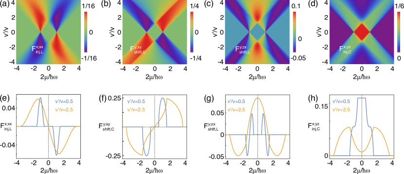
Figure 2: ${\cal F}^{c;ab}$ of a tilted Weyl point in three dimensions. (a,e) $x;xx$ component of the linear injection. (b,f) $y;xy$ component of the circular shift. (c,g) $y;zx$ component of the linear shift. (d,h) $x;yz$ component of the circular injection. Since we take $\omega>0$, the sign of $2\mu/\hbar\omega$ here should be understood as the sign of the chemical potential $\mu$.

Figure 2 shows some representative components calculated from quantum geometric quantities by Eqs. (18), (IV.1), and (36). There are some features that need to be discussed. First, as we explained in Sec. III only the circular injection current is nonvanishing at the neutral filling $\mu=0$ in the type-I case where $|v^{\prime}/v|<1$. It is because, in this case, the Fermi surface is a point, so anisotropic excitation cannot occur. The circular injection response is quantized because of the quantized Berry curavature from a Weyl point, as found in Ref. [5] [See Eq.  (18)]. Other responses are significant near $\hbar\omega=2\mu$, where the anisotropic excitation occurs.

However, there are significant differences between the $PT$-symmetric responses and the linear shift response. $PT$-symmetric responses have peaks at $\hbar\omega=|2\mu|$, i.e., when the excitation occurs on a full hemisphere, while $T$-symmetric responses vanish at $\hbar\omega=|2\mu|$ and changes sign there [13]. For the linear injection current, the peak at $\hbar\omega=|2\mu|$ is natural because the transition of the electron velocity during the excitation from the valence band $v$ to the conduction band $c$, $\Delta^{x}_{cv}=v^{x}_{c}-v^{x}_{v}$, is all positive or all negative on the hemisphere. There is no simple analogous way to understand the trend of shift current response based on the shift vector, but the vanishing of the linear shift current response at $\hbar\omega=|2\mu|$ can be attributed to the $T$-symmetric nature. Since $T$ symmetry requires that the current generated from one hemisphere equal to the current generated from the other hemisphere, both hemisphere should generate zero currents because linear shift currents are not generated when excitations occur on the full sphere. There are also interesting differences between the $PT$-symmetric responses and $T$-symmetric responses at $\mu=0$ in the type-II case where $|v^{\prime}/v|>1$. As explained in Sec. III, emergent $CPT$ symmetry at $\mu=0$ requires that the former has a vanishing response while the latter can have a nontrivial response. In other words, $PT$-symmetric responses do not distinguish type-I and type-II cones at $\mu=0$ whereas $T$-symmetric responses distinguish them.

As we understand a single Weyl point, it is straightforward to extend our knowledge to Dirac points in two and three dimensions. In both 2D and 3D, the protection of a Dirac point requires $PT$ symmetry. In 2D, the Dirac Hamiltonian has the form $H_{\rm 2D}=-\mu-\hbar v^{\prime}k_{x}+\hbar v(k_{x}\tau_{x}+k_{y}\tau_{y})$, where $\tau_{i=x,y,z}$ are Pauli matrices for the orbital degrees of freedom, and spinless $PT=\sigma_{z}K$ symmetry forbids the mass term $m\sigma_{z}$. In 3D, the Dirac Hamiltonian has the form $H_{\rm 3D}=-\mu-\hbar v^{\prime}k_{x}+\hbar v(k_{x}\tau_{x}+k_{y}\tau_{y}\sigma_{x}+k_{z}\tau_{z})$, and the twofold degeneracy (Kramers degeneracy) of bands at every momentum require $PT=i\sigma_{y}K$ symmetry. Here, $\tau_{i=x,y,z}$ and $\sigma_{i=x,y,z}$ are Pauli matrices for the orbital and spin degrees of freedom, respectively. In 3D, even in the presence of $PT$ symmetry, two mass terms are allowed, which are $m_{1}\tau_{y}\sigma_{y}$ and $m_{2}\tau_{y}\sigma_{z}$. We need threefold or fourfold rotational symmetry to protect the Dirac point in 3D by disallowing mass terms. Our massless Dirac model have continuous $\theta$ rotational symmetry around the $x$ axis under $C_{\theta}=e^{i\theta(\sigma_{x}+\tau_{x}\sigma_{x}/2)}$, satisfying $C_{\theta}H({\bf k})C_{\theta}^{-1}=H(C_{\theta}{\bf k})$. Keeping either threefold $C_{3x}$ or fourfold $C_{4x}$ rotational symmetry in crystals preserves the gap closing [65, 66, 52], which we assume here. Because gapless Dirac points have $PT$ symmetry, they can only have linear injection or circular shift current responses. These responses have the same pattern shown for a Weyl point.

Here we emphasize again that while multiple responses coexist in magnetic Weyl and Dirac semimetals, each response occurs through different components of the conductivity. This helps measure each response separately. In particular, it facilitates the measurement of the circular shift current in magnetic Dirac and Weyl semimetals. Table. 2 and Eq. (III.1) shows that the current generated along the $y$ direction under the illumination of circularly polarized light propagating in the $z$ direction is only the circular shift currents. The photocurrent along the $y$ direction should thus be identified with the circular shift current.

V.2 Dirac surface state

As an application to a more realistic model with ${\bf k}$-nonlinear terms, we study the single Dirac surface state of magnetic topological insulators. Let us begin with the following effective Hamiltonian studied in Refs. [23, 24].

$$H =-\mu+\frac{\hbar^{2}k^{2}}{2m}+\hbar v\left(k_{x}\sigma_{y}-k_{y}\sigma_{x}\right)+\Delta\sigma_{y}.$$ (43)

Here, $\Delta\neq 0$ is due to spin ordering along the $y$ direction, and it breaks $M_{x}=i\sigma_{x}$, rotation $C_{2z}=-i\sigma_{z}$, and time reversal $T=i\sigma_{y}K$ symmetries. Since this in-plane ordering preserves $C_{2z}T$ symmetry, it does not open the gap, and it just shifts the location of Dirac points by $-\Delta/\hbar v$ from the time-reversal-invariant momentum. The shifting tilts the Dirac cone because of the quadratic term: if we write $(k_{x},k_{y})=(-\Delta/\hbar v+q_{x},q_{y})$, the Hamiltonian has the form $H=-\mu-(\hbar\Delta/mv)q_{x}+\hbar v\left(q_{x}\sigma_{y}-q_{y}\sigma_{x}\right)$ up to linear order in $q$, which is studied above. Assuming $C_{3z}$ symmetry of the nonmagnetic state, we add a hexagonal warping term in order to account for the crystalline symmetry of the real system.

$$h_{\rm warp} =\lambda(k_{x}^{3}-3k_{x}k_{y}^{2})\sigma_{z}.$$ (44)

This term breaks $M_{y}=i\sigma_{y}$ symmetry and $C_{2z}T$ symmetry that are preserved by the spin ordering, so it opens small band gap (about $0.8$ meV for parameters given below). Since $T$ and $C_{2z}T$ symmetries are both broken, all four types of shift and injection currents can be generated in this system. However, the residual $M_{x}T$ symmetry imposes that the separation of responses remains exact: nonvanishing components of the conductivity are $\sigma^{y;xx}_{\rm shift,L}$, $\sigma^{y;yy}_{\rm shift,L}$, $\sigma^{x;xy}_{\rm shift,L}$ for linear shift current, $\sigma^{x;xx}_{\rm inj,L}$, $\sigma^{x;yy}_{\rm inj,L}$, $\sigma^{y;xy}_{\rm inj,L}$ for linear injection current, $\sigma^{y;xy}_{\rm shift,C}$ for circular shift current, and $\sigma^{x;xy}_{\rm inj,C}$ for circular injection current.

For a numerical calculation, we take $\mu=50$ meV, $m=0.13m_{e}$ where $m_{e}$ is the free electron mass, $\hbar v=2.5\;{\rm eV\AA^{-1}}$, $\lambda=250\;{\rm eV\AA^{-3}}$, and $\hbar\tau^{-1}=1$ meV and use Eqs. (18) and (22). Figure 3 show the calculated photoresponsivity $\kappa^{c;ab}=2\sigma^{c;ab}/\epsilon_{0}c$, which has the dimension of the photocurrent density per unit intensity of light [57]. The peak value (occurring at $\hbar\omega\sim 2\mu=100$ meV) of the linear injection part is the strongest, and the others are smaller by two orders of magnitude. However, since the circular shift current grows as $\omega^{-2}$ while the linear injection current grows as $\omega^{-1}$, the circular shift current can be comparable to or larger than the linear injection current when the peak is located below $10$ meV. On the other hand, the small-frequency divergence of the linear shift current is weaker because it is due to $\lambda\neq 0$ [10] and is not from the tilting, and thus the peak value scales like $O(\omega^{0})$ as $\mu$ is lowered. Therefore, the $y$ component photocurrent generated by a circularly polarized light, $j^{y}=(\kappa^{yxx}_{\rm shift,L}+\kappa^{yyy}_{\rm shift,L}-2\kappa^{y;xy}_{\rm shift,C})I$, is dominated by the circular shift ($\kappa^{y;xy}_{\rm shift,C}$) current when $\hbar\omega\sim 2\mu<100$ meV. The magnitude of the linear shift current and the circular shift current can be compared in experiments since the circular parts can be measured from the current difference between the left-circularly polarized light and the right-circularly polarized light.

In experiments, the value of the observed photocurrents can be smaller than the value predicted here. For example, the photocurrents observed in Ref. [24] shows photoresponsivity of about $5\;{\rm nAcm^{-1}W^{-1}}$ at $\omega\sim 250$ meV, which is two orders of magnitude smaller than the calculated value here. While several factors can contribute to this reduction, one is from the cancellation between the top and bottom surfaces. This cancellation can be reduced by increasing the thickness of the sample because light attenuates more while propagating within the bulk such that the photocurrent is generated significantly on only one surface that is directly illuminated.

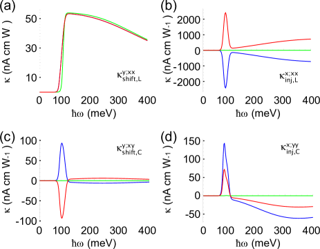
Figure 3: Photoresponsivity of the magnetic Dirac surface state. $\mu=50$ meV, $m=0.13m_{e}$, $\hbar v=2.5\;{\rm eV\AA^{-1}}$, $\lambda=250\;{\rm eV\AA^{-3}}$, and $\hbar\tau^{-1}=1$ meV. Blue, green, and red curves correspond to $\Delta=30$ meV, $0$ meV, and $-30$ meV, respectively. $\kappa^{c;ab}=1\;{\rm nAcmW^{-1}}$ is equivalent to $\sigma^{c;ab}=1.33\;{\rm pAcm^{-1}V^{-2}}$.

VI First-principles calculations for real topological semimetals

For further demonstrations of our theory beyond simple two-band models, we perform first-principles calculations on the shift and injection photocurrent conductivities as well as geometric quantities of antiferromagnetic MnGeO₃ and ferromagnetic PrGeAl, respectively, as representatives of real magnetic Dirac and Weyl semimetals. We notice that such calculations on the bulk photovoltaic effects in real magnetic topological semimetal have not been reported yet despite the fact that topological semimetals are expected to be efficient infrared and terahertz photodetectors [1].

VI.1 Antiferromagnetic Dirac semimetal MnGeO₃

MnGeO₃ forms a centrosymmetric rhombohedral structure [see Fig. 9(a)] with space group $R\overline{3}$ [67], and consequently, it would not exhibit any bulk photovoltaic effects. Interestingly, it becomes antiferromagnetic below 38 K [67] and the AF structure (magnetic space group $-3^{\prime}$) [see Fig. 9(a)] breaks both $T$ and $P$ symmetries while preserving the combined $PT$ symmetry [42], thus leading to AF-induced bulk photovoltaic effects with linear injection and circular shift currents (see Table I). Furthermore, it was recently predicted to be a Dirac semimetal with $PT$ symmetry-protected Dirac points (DPs) [42].

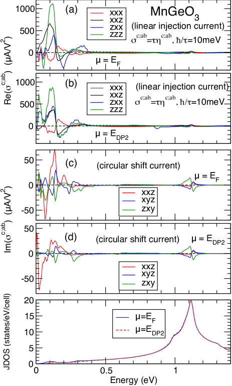
Figure 4: Conductivity tensors and joint density of states (JDOS) of antiferromagnetic MnGeO₃. (a, b) Linear injection. (c, d) Circular shift. In (b) and (d), the conductivities are calculated with the Fermi level set to the DP₂ Dirac point energy (see Fig. 5). (e) JDOS as a function of photon energy.

In AF MnGeO₃, because of its $PT$ symmetry, there are only nonvanishing circular shift photocurrent and linear injection photocurrent, as mentioned before (see Table I). Furthermore, the $-3^{\prime}$ magnetic space group admits only three nonvanishing independent matrix elements (i.e., $xxz=-xzx=yzy$, $xyz=-xzy=-yxz$ and $zxy=-zyx$) of the circular shift conductivity tensor and six nonvanishing independent matrix elements (i.e., $xxx=-xyy=-yxy$, $xyz=-yxz$, $xxz=yyz$, $xxy=yxx=-yyy$, $zxx=zyy$ and $zzz$) of the linear injection conductivity tensor [51]. Hereafter we use the shorthand notation $cab$ for $\sigma^{c;ab}$. We display these nonvanishing conductivity elements in the low photon energy range in Fig. 4. For simplicity, we plot only the four pronounced $xxx$, $xxz$, $zxx$ and $zzz$ elements of the linear injection conductivity tensor in Fig. 4. $\hbar\tau^{-1}$ = 10 meV is assumed. We notice that the magnitudes of the linear injection conductivity elements ($\sigma^{c;ab}$) are gigantic in the photon energies below 0.25 eV (Fig. 4). The magnitudes are order of $\tau e^{3}/(2\pi\hbar^{2})=500$ $\mu$A/V², which are one order of magnitude larger than those in architypical polar semiconductors CdS and CdSe [68]. Circular shift photocurrents (Fig. 4) are also 10 times larger than linear shift currents in semiconductors CdS and CdSe [68]. This is remarkable because it demonstrates that the AF magnetism-induced linear injection and circular shift photocurrents, respectively, can be as large as circular injection and linear shift currents in nonmagnetic noncentrosymmetric materials. Furthermore, this means that the photocurrents in AF semimetals can be controlled via manipulating the magnetism with, e.g., an applied magnetic field [26].

AF MnGeO₃ hosts at least three DPs near the Fermi level $E_{F}$ along the $k_{z}$ axis, as shown in Fig. 5. In particular, there is a DP just above $E_{F}$ (at 1.7 meV) and being located close to the $\Gamma$ point [at ${\bf k}_{DP1}=(0,0,-0.00364)2\pi/a$]. This could explain the large values of the calculated photocurrents, as shown in Figs. 4(a) and 4(c). To further examine the important contributions of the DPs to the photocurrents, we also calculate the conductivity spectra with the Fermi level set to the DP2 Dirac point energy (i.e., $E=46.5$ meV). DP2 is located at ${\bf k}_{DP1}=(0,0,0.11112)2\pi/a$ above the $k_{z}=0$ plane in the $k$-space [see Fig. 5(a)]. We notice that both the shapes and magnitudes of all the conductivity spectra except conductivity element $\sigma^{xxz}$, roughly remain the same. For example, the gigantic peak of about 1000 $\mu$A/V² at $\sim$100 meV in the Re($\sigma^{zzz}$) linear injection current spectrum appears in both cases [see green curves in Figs. 4(a) and 4(b)]. Nonetheless, its sharp negative peak at 50 meV disappears in the case where the chemical potential $\mu$ is tuned to $\mu=E_{DP2}$ and a sharp positive peak of larger than 700 $\mu$A/V² occurs at 20 meV instead. Interestingly, there is a sharp positive peak at photon energy of 5 meV in the Im($\sigma^{xxz}$) circular shift current calculated by setting $\mu=E_{DP2}$. This is due to the $\omega^{-1}$ behavior of the shift conductivity near the Dirac point. Comparing red curves in Figs.1 (c) and (d) for Im($\sigma^{xxz}$), one can also see that the large negative peak moves from photon energy 65 meV to 25 meV [see Fig. 4(d)].

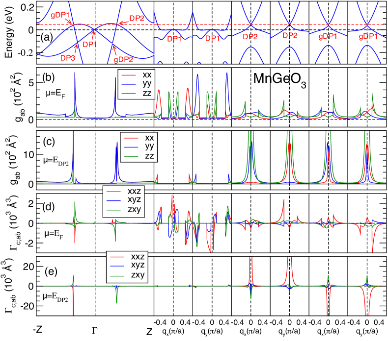
Figure 5: Enhancement of geometric quantities near Dirac points. (a) Energy bands along the $k_{z}$ axis from $-\pi/c$ to $\pi/c$ ($Z=\pi/c$) and also along the $k_{x}$ and $k_{y}$ directions through the DP1 and DP2 Dirac points as well as the gDP1 gapped Dirac point. (b) and (c) Quantum metric ($g_{ab}$) along the same symmetry lines as in (a), calculated for the Fermi energy ($E_{F}$) and the DP2 energy ($E_{DP2}$), respectively. (d) and (e) The same as in (b) and (c), respectively, but for Christoffel symbol of the first kind ($\Gamma_{c;ab}$). Here ${\bf q}={\bf k}-{\bf k}_{DP}$ denotes the momentum displacement from a DP (qDP) point.

While an enhanced joint density of states (JDOS), $\rho(\omega)=\int_{\bf k}\sum_{m,n}f_{nm}\delta(\omega_{mn}-\omega)$, is a possible origin of large conductivity tensors in insulators [57], it cannot explain the peaks shown here. Figure 4(e) shows that JDOS is suppressed at low-frequencies rather than being enhanced. As we show above, linear injection and circular shift currents are, respectively, related to geometric quantities quantum metric ($g_{ab}$) and Christoffel symbols of the first kind ($\Gamma_{c;ab}$) at low-energies through Eq. (IV.4). Thus, the large enhancement of conductivity tensors has geometric origin. To demonstrate this, we display $g_{ab}$ and $\Gamma_{c;ab}$ at $\mu=E_{F}$ and also at $\mu=E_{DP2}$ along the symmetry lines in Fig. 5. For most of the DPs, a DP is associated with a gapped DP (gDP) located approximately at the inverted position in the $k$-space. For example, the associated gPD for DP2 is gDP1 at ${\bf k}_{DP1}=(0,0,-0.11051)2\pi/a$, and the DP2 energy level falls within the gDP1 band gap [see Fig. 5(a)]. On the other hand, there is no gDP associated with DP1. Figures 5(b) and 5(d) clearly show that for $\mu=E_{F}$, $g_{ab}$ and $\Gamma_{c;ab}$ have sharp peaks near DP1 along the $k_{x}$ and $k_{y}$ directions. $g_{xx}$ and $g_{yy}$ also peak sharply at the positions of the DP2 and gDP1 along the $k_{z}$ axis even though $\mu=E_{F}\neq E_{DP2}$. This indicates that the gigantic linear injection and circular shift currents stem, respectively, from the large values of the quantum metric and Christoffel symbol in the vicinity of the DP1 Dirac point. Furthermore, $g_{zz}$ has prominent peaks in the vicinity of (but slightly away from) the DP2 and gDP1 points along the $k_{x}$ and $k_{y}$ directions, which are mainly caused by the interband transitions from the lower (occupied) Dirac cone to higher (empty) Dirac cone with transition energies of $\sim$0.1 eV [see Fig. 5(b)]. These $g_{zz}$ peaks thus give rise to the gigantic peak in linear injection current Re($\sigma^{zzz}$) at around 0.1 eV [see green curves in Fig. 4(a)].

For $\mu=E_{DP2}$, as expected, $g_{ab}$ and $\Gamma_{c;ab}$ exhibit sharp peaks close to both the DP2 and gDP1 points [see Figs. 5(c) and 5(e)]. In particular, $g_{zz}$ has huge positive peaks near the DP2 and gDP1 points along all three cartesian coordinate directions, thus resulting in the prominent peak at 0.1 eV in linear injection conductivity Re($\sigma^{zzz}$) [Fig. 4(b)], as in the $\mu=E_{F}$ case [Fig. 4(a)]. Nevertheless, Fig. 5(e) shows that the $\Gamma_{c;ab}$ peaks near the DP2 and gDP1 have the opposite signs. This could explain why the circular shift conductivity elements Im($\sigma^{xyz}$) and Im($\sigma^{zxy}$) become smaller when the Fermi level is raised from $E_{F}$ to $E_{DP2}$ [Figs. 4(c) and 4(d)] because the contributions from the DP2 and gDP1 cancel each other to some extent. In contrast, the linear injection current elements remain almost unchanged mainly because the $g_{ab}$ peaks have the same signs. Nonetheless, there is a huge peak in the $\Gamma_{xxz}$ at gDP1, which is absent at DP2, because now the Fermi level falls within the gDP1 gap [see Fig. 5(e)]. This results in the large low energy peaks in the Im($\sigma^{xxz}$) conductivity element [see red curves in Fig. 4(d)].

VI.2 Ferromagnetic Weyl semimetal PrGeAl

PrGeAl forms a body-centered tetragonal structure (see Fig. 9b) with noncentrosymmetric space group $I4_{1}md$ and point group $4mm$. [69] It becomes ferromagnetic at $T_{C}=16$ K [44] and the FM structure (Fig. 9b) has no $T$ symmetry nor $PT$ symmetry. Therefore, all four types of photocurrents may emerge in FM PrGeAl (Table I). Interestingly, it was recently predicted to be a rare ferromagnetic noncentrosymmetric Weyl semimetal [43]. Furthermore, the Weyl nodes and surface Fermi arcs in PrGeAl were observed in very recent photoemission spectroscopy experiments [44]. Thus, FM PrGeAl provides a valuable platform for studying all types of bulk photovoltaic effects in Weyl semimetals.

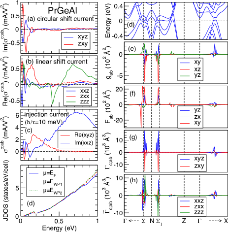
Figure 6: Conductivity tensors and geometric quantities in ferromagnetic PrGeAl. (a, b) Shift and (c) Injection conductivity tensors. (d) JDOS as a function of photon energy. The cases with $\mu=E_{\rm WP1}$ and $\mu=E_{\rm WP2}$ are also shown. (e) Energy bands, (f) quantum metric $g_{ab}$, (g) Berry curvature $F_{ab}$, (h) Christoffel symbol $\Gamma_{c;ab}$, and (i) symplectic Christoffel symbol $\widetilde{\Gamma}_{c;ab}$ along the high symmetry lines in the Brillouin zone [see Fig. 9(d) in Appendix L].

The crystalline point group of PrGeAl is $4mm$. Thus, there are three inequivalent nonvanishing matrix elements (i.e., $xxz=yyz$, $zxx=zyy$ and $zzz$) of linear shift conductivity and one nonvanishing element ($xxz=yyz=-xzx=-yzy$) of circular injection conductivity in PrGeAl above $T_{C}=16$ K. [51]. The magnetic point group of FM PrGeAl is $4m^{\prime}m^{\prime}$. Consequently, in addition, there are two nonvanishing elements (i.e., $xyz=-xzy=-yxz$ and $zxy=-zyx$) of circular shift conductivity and one nonvanishing element ($xyz=-yxz$) of linear injection conductivity in PrGeAl below $T_{C}$. [51] Here, the presence of $M_{x}T$ and $M_{y}T$ symmetries forbids linear shift and injection conductivities to be simultaneously nonvanishing in the same component. The same is true for the circular polarization. The calculated conductivity spectra of these nonvanishing matrix elements are displayed in Fig. 6. We notice that all the shift current elements have large peaks below photon energy 0.25 eV [see Figs. 6(a) and 6(b)]. This is due to the $\omega^{-1}$ enhancement of the shift conductivity tensors at low frequencies. Indeed, the magnitudes of these peaks below 0.1 eV are comparable to those in architypical nonmagnetic Weyl semimetal TaAs [16], which also has the $I4_{1}md$ space group. Linear shift current element Re($\sigma^{zzz}$) is also large in the higher energy range between 0.4 eV and 1.0 eV. This peak is not due to magnetic order because it is observed in $T$-symmetric responses. It is hardly related with the responses of Weyl points. The peak is far from the Fermi level, and also the conductivity components showing the large peaks is not generated by linearly dispersing Weyl points [See Table. 2 for example]. We do not aim to explain its origin here. The calculated circular shift conductivity elements below 0.2 eV are comparable to that of the linear shift current (Fig. 6), and remarkably, are one order of magnitude larger than those in AF Dirac semimetal MnGeO₃ [see Figs. 4(c) and 4(d)]. No first-principles calculation of circular shift current in other semimetals has been reported yet.

Similar to the linear shift conductivity, circular injection conductivity Im($\sigma^{xxz}$) has a gigantic broad peak between 0.5 eV and 1.0 eV, and the peak value is almost one order of magnitude larger than that of linear injection conductivity in AF MnGeO₃ (see Fig. 4). It also has large peaks below 0.15 eV, although the magnitudes of these peaks are a few times smaller than the gigantic peak in the higher energy region. Linear injection conductivity Re($\sigma^{xyz}$) in FM PrGeAl is also large and is about ten times larger than that of AF MnGeO₃ in the very low energy region. This one order of magnitude enhancement can be related to the presence of many Weyl points, as we analyze further below.

As in MnGeO₃, JDOS is suppressed at low energies [Fig. 6(d)] Thus, the origin of the large low-frequency photocurrents should be attributed to the geometric enhancement. We have calculated all four geometric quantities along the symmetry lines in the Brillouin zone [Fig. 9(d)], as displayed in Fig. 6. We find that all four quantities have sharp peaks in the vicinity of the $\Sigma$ and $\Sigma_{1}$ points, where there are several anticrossing nodal points with the Fermi level falling within their gaps [see Fig. 6(e)]. Since these gaps near the anticrossing points are mostly within 0.1 eV, the large peaks in the geometric quantities thus give rise to the sharp photoconductivity peaks around 0.1 eV and below. In particular, Christoffel symbols $\Gamma_{xyz}$ and $\Gamma_{zxy}$ have gigantic peaks near the $\Sigma$ and $\Sigma_{1}$ points with the same signs, thus resulting in sharp peaks in circular shift conductivities Im($\sigma^{xyz}$) and ($\sigma^{zxy}$), respectively, below photon energy 0.1 eV [Fig. 6(a)].

FM PrGeAl has been reported to be a rare noncentrosymmetric FM Weyl semimetal with at least 160 Weyl points (WPs) within $\pm$0.1 eV of the Fermi level [43]. Furthermore, there are both type I and II WPs among them. Here we consider two WPs, one type I and the other type II, and study their influences on the photocurrents. The type I WP (WP1) sits at ${\bf k}=(0.160,0.204,-0.003)2\pi/a$ in the BZ and is located at 53.9 meV above $E_{F}$ ($E_{\rm WP1}$). The type II WP (WP2) is at ${\bf k}=(0.015,0.255,0.217)2\pi/a$ and its energy is 67.4 meV above $E_{F}$ ($E_{\rm WP2}$). They correspond, respectively, to Weyl points W${}^{1}_{3}$ and W${}^{1}_{2}$ reported in Ref. [43]. To study the influences of the WPs on the photocurrents, we calculate all the nonvanishing conductivity elements and all the geometric quantities with the Fermi level set to $E_{\rm WP1}$ and also to $E_{\rm WP2}$.

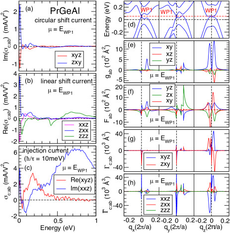
Figure 7: Same as in Fig. 6, but with $\mu=E_{\rm WP1}$. (a, b) Shift and (c) Injection conductivity tensors. (d) Energy bands, (e) quantum metric $g_{ab}$, (f) Berry curvature $F_{ab}$, (g) Christoffel symbol $\Gamma_{c;ab}$, and (h) symplectic Christoffel symbol $\widetilde{\Gamma}_{c;ab}$ along the three cartesian coordinate axis directions through the WP1 Weyl point ($E=E_{\rm WP1}$). Here ${\bf q}={\bf k}-{\bf k}_{\rm WP1}$ denotes the momentum displacement from the WP1 point.

The conductivity and geometric quantity spectra obtained by setting the Fermi level to the WP1 Weyl point energy ($E_{\rm WP1}$) are plotted in Fig. 7. Remarkably, compared with the $\mu=E_{F}$ case in Fig. 6, all the photoconductivity elements within the photon energy of 50 meV increase by a factor of 2 or more. In particular, linear shift conductivity element Re($\sigma^{zxx}$) is enhanced by a factor of 5 [Fig. 7(b)]. Other changes include that the peak at $\sim$70 meV in circular shift conductivity elements Im($\sigma^{xyz}$) and Im($\sigma^{zxy}$) get significantly reduced [Fig. 7(a)] and that the positive peak at $\sim$40 meV in linear shift conductivity element Re($\sigma^{zzz}$) changes to the negative peak [Fig. 7(a)]. Nonetheless, the features of all the conductivity elements above 100 meV remain essentially unchanged.

The changes caused by moving the Fermi level to the WP1 WP energy mentioned above, can be largely explained by the distributions of the four geometric quantities in the vicinity of the WP1 Weyl point, as displayed in Figs. 7(e), 7(f), 7(g) and 7(h). For example, symplectic Christoffel symbol $\widetilde{\Gamma}_{zxx}$ has high positive peaks along all three coordinate directions near the WP1 WP [see Figs. 7(h)]. These peaks thus give rise to the five-fold increased linear shift conductivity Re($\sigma^{zxx}$). Note that although in the $\mu=E_{F}$ case $\widetilde{\Gamma}_{zxx}$ also has sharp peaks near the $\Sigma$ and $\Sigma_{1}$ points, these peaks have both positive and negative signs [see Figs. 6(i)] and thus their contributions to the linear shift conductivity cancel each other to some extent.

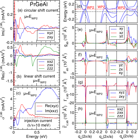
Figure 8: Same as in Fig. 6, but with $\mu=E_{\rm WP2}$. (a, b) Shift and (c) Injection conductivity tensors. (d) Energy bands, (e) quantum metric $g_{ab}$, (f) Berry curvature $F_{ab}$, (g) Christoffel symbol $\Gamma_{c;ab}$, and (h) symplectic Christoffel symbol $\widetilde{\Gamma}_{c;ab}$ along the three cartesian coordinate axis directions through the WP2 Weyl point $E=E_{\rm WP2}$. ${\bf q}={\bf k}-{\bf k}_{\rm WP2}$ denotes the momentum displacement from the WP2 point.

The results obtained by setting the Fermi level to the energy of the type II WP2 Weyl point are plotted in Fig. 8. We notice that as for the WP1 WP case, all the photoconductivity spectra remain more or less unchanged for photon energies larger than 100 meV. As for the WP1 WP case, the peak height of linear shift conductivity Re($\sigma^{zxx}$) at very low energy of $\sim$10 meV gets doubled, although the sign of the peak changes from positive to negative [see Fig. 8(b)]. However, in contrast to the WP1 Weyl point case, many low energy peaks especially of shift current conductivity elements, become smaller [Figs. 8(a) and 8(b)]. In particular, the peak at 10 meV in both circular shift elements Im($\sigma^{xyz}$) and Im($\sigma^{zxy}$) decreases by a factor of nearly 2, and also the peak sign changes to the opposite. These different changes in the low energy photoconductivity spectra betwen the type I and type II Weyl point cases may be attributed to their different energy dispersions and hence the different distributions of the four geometric quantities near the Weyl points (see Figs. 7 and 8). Figure 7(d) shows that in the type I WP1 case, the upper and lower Weyl cone bands lie, respectively, above and below the WP1 energy. As a result, the low energy inter-Weyl-band transitions may occurr in all three coordinate directions when the Fermi level is set to $E_{\rm WP1}$. This can result in large peaks in the four geometric quantities near the WP1 Weyl point, thus leading to the many fold enhancements in photocurrents, as discussed above. In the type II WP2 Weyl point case, in contrast, both upper and lower Weyl bands along the $-k_{x}$ and $+k_{y}$ directions lie below $E_{\rm WP2}$ [see Fig. 8(d)]. This hinders the low energy inter-Weyl-band transitions along these two directions when $E_{F}$ is set to $E_{\rm WP2}$, and thus reduces the peaks in the geometric quantities near the WP2 point, thereby leading to several smaller peaks in the photocurrents below $\sim$20 meV. Of course, in a real topological semimetal such as the present system, situation could be more complicated. Figure 8(d) shows that other bands may come quite close to the WP2 Weyl point in energy and they thus enable, e.g., the transitions from two Weyl bands below $E_{\rm WP2}$ to the other bands above $E_{\rm WP2}$ along the $-k_{x}$ and $+k_{y}$ directions, thus also giving rise to prominent peaks in the geometric quantities near the WP2 point [see Figs. 8(e), 8(f), 8(g) and 8(h)].

VII Discussion

Let us discuss some issues related to the smallness of the frequency. We note that our theory is reliable for the photon frequency above 1 THz because we assume $\omega\gg\Gamma.$ Since the typical relaxation time in semimetals is one picosecond, $\omega/2\pi>1$ THz should be taken for our theory to apply. Thus, the divergence of the responses in our model should not be interpreted as a physical divergence, and it is cut off at $\omega\sim\Gamma$. Moreover, intraband (i.e., non-transitive) second-order optical responses exist in magnetic systems, and they become comparable to the interband responses when $\omega\lesssim\Gamma$. To estimate the magnitude of the intraband responses, let us consider the semiclassical second-order optical response $\sigma^{c;ab}_{\rm SC}(\omega)=-(e^{3}/\hbar^{2})(\omega^{2}+\Gamma^{2})^{-1}\sum_{n}\int_{\bf k}f^{\rm FD}_{n}\partial_{a}\partial_{b}v^{c}_{n}$. It has the same symmetry property as the linear injection current (so it appears in magnetic systems where time-reversal symmetry is broken) and scales as $\omega^{-2}\mu^{2-d}$ near tilted Dirac or Weyl points. Since the $\omega^{-2}$ factor enhances the semiclassical response at low-frequences, it becomes comparable to the peak value of the linear injection response at $\omega\lesssim\tau^{-1}=\Gamma$ if we take $\mu~{}\sim\omega$.

Another thing to care about at low frequencies is the validity of the perturbation theory. We suppose that the photovoltaic responses are dominated by the second-order responses since the electric field is generally weak enough. However, at small frequencies, $A=E/\omega$ becomes large, so higher-order responses can become significant. According to the Floquet theory analysis in Ref. [4], perturbation theory works well for $\left|\omega^{-1}eEv\right|\ll\hbar\Gamma$, where we assume that the interband velocity matrix element has the same order of magnitude as the intraband velocity. It sets a lower bound for $\omega$. For $\hbar v\sim 1\;{\rm eV\AA^{-1}}$ and $\Gamma\sim 1$ THz, the lower bound is $\omega_{\rm min}\approx\sqrt{I/({\rm W/cm^{2}})}{\rm\;THz}$. While this bound is very small for typical lasers with intensity $I<1\;{\rm W/cm^{2}}$, it should be taken into account for an analysis of the experimental results obtained by using high-intensity pulse lasers.

In the non-perturbative regime, light absorption occurs faster than the interband relaxation, so electrons are excited until the system reaches a new equilibrium where the absorption and emission of light finds a balance. The relaxation plays an important role here because a mismatch between the absorption and emission, which generate opposite photocurrents, requires a finite relaxation [4]. Even in a very clean system with an extremely small $\Gamma$, the low-frequency divergent behavior we discuss above is cut off by this reason.

At finite temperature, thermal fluctuation can significantly reduce low-frequency photovoltaic response in tilted-Dirac or Weyl semimetals [13]. When the peak value is considered, the relevant frequency scale where the peak value is reduced to half is $2|v/v^{\prime}|k_{B}T/\hbar$ for type I and $2k_{B}T/\hbar$ for type II. It sets a quite high lower-bound, since $2k_{B}T/\hbar=$12 THz at room temperature (cf. 0.17 THz at 4.2K and 3.2 THz at 77 K). When the tilting is small such that $|v^{\prime}/v|<0.4$, the cut-off scale is larger than $30\;{\rm THz}$ at room temperature, which is the highest edge of the terahertz radiation. Therefore, cooling will be needed in order for tilted-Dirac or Weyl semimetals to work as an efficient terahertz photodetector.

Throughout this work, we focus on the DC generation. However, let us note that our results can also be applied to the second harmonic generation, where an alternating current of frequency $2\omega$ is generated by a uniform illumination of light with frequency $\omega$. Since the second harmonic generation is associated with the shift vector [4, 13], its low-energy divergence has the same form as that for the shift current [13], and thus it can be related to the quantum geometric connection. We believe that similar geometric interpretations of other quantities are also possible. It will be an interesting topic to explore quantum geometric properties of the third-order optical conductivity. Since it has four components, we expect the existence of a third-order optical response controlled by the Riemann curvature tensor $R^{a}_{bcd}=\partial_{c}\Gamma^{a}_{db}-\partial_{d}\Gamma^{a}_{cb}+\sum_{e}(\Gamma^{a}_{ce}\Gamma^{e}_{db}-\Gamma^{a}_{de}\Gamma^{e}_{cb})$.

Note added.— Recently, Hikaru Watanabe and Yoichi Yanase studied the bulk photovoltaic responses in magnetic systems independently of ours. They also figure out the circular shift current and discuss its enhancement near gap-closing points. Our results are consistent with the results in their preprint when there is an overlap.

Appendix A Conventions and Definitions

• We do not distinguish uppercase and lowercase indices except for the Christoffel symbols.

• $-e$ is the electron charge. $e>0$.

• Geometric quantities on the Bloch sphere (indices $i=1,2,3$ are for the $(f_{1},f_{2},f_{3})$ basis):

  $$\eta_{ij}$$ metric tensor

  $$\epsilon_{ij}$$ symplectic form

  $$q_{ij}=\eta_{ij}-i\epsilon_{ij}$$ quantum geometric tensor

  $$\gamma^{i}_{jk}$$ Christoffel symbol of the second kind

  $$\gamma_{ijk}$$ Christoffel symbol of the first kind

  $$\tilde{\gamma}_{ijk}$$ symplectic Christoffel symbol

  $$c_{ijk}=\gamma_{ijk}-i\tilde{\gamma}_{ijk}$$ quantum geometric connection (45)

• Geometric quantities in momentum space (indices $a=1,2,3$ are for the $(k_{1},k_{2},k_{3})$ basis)

  $$g_{ab}$$ metric tensor

  $$F_{ab}/2$$ symplectic form

  $$Q_{ab}=g_{ab}-iF_{ab}/2$$ quantum geometric tensor

  $$\Gamma^{a}_{bc}$$ Christoffel symbol of the second kind

  $$\Gamma_{abc}$$ Christoffel symbol of the first kind

  $$\tilde{\Gamma}_{abc}$$ symplectic Christoffel symbol

  $$C_{abc}=\Gamma_{abc}-i\tilde{\Gamma}_{abc}$$ quantum geometric connection (46)

• Typical quantities in second-order optical conductivity.

  $$\partial_{a} =\frac{\partial}{\partial_{k_{a}}},$$

  $$\int_{\bf k} =\int\frac{d^{3}k}{(2\pi)^{3}},$$

  $$\omega_{n} =\hbar^{-1}\braket{n}{H}{n},$$

  $$v^{a}_{mn} =\hbar^{-1}\braket{m}{\partial_{a}H}{n},$$

  $$w^{ab}_{mn} =\hbar^{-1}\braket{m}{\partial_{a}\partial_{b}H}{n},$$

  $$u^{abc}_{mn} =\hbar^{-1}\braket{m}{\partial_{a}\partial_{b}\partial_{c}H}{n},$$

  $$f^{\rm FD}_{m} =\text{Fermi-Dirac distribution of the $m$th band},$$

  $$\omega_{mn} =\omega_{m}-\omega_{n},$$

  $$f^{\rm FD}_{mn} =f^{\rm FD}_{m}-f^{\rm FD}_{n},$$

  $$\Delta^{a}_{mn} =v^{a}_{mm}-v^{a}_{nn},$$

  $$R^{c;a}_{mn} =r^{c}_{mm}-r^{c}_{nn}+i\partial_{c}\log r^{a}_{mn},$$

  $$r^{a}_{mn} =i\braket{m}{\partial_{a}}{n},$$

  $$r^{a}_{mn;c} =\partial_{c}r^{a}_{mn}-i(r^{c}_{mm}-r^{c}_{nn})r^{a}_{mn}.$$ (47)

Appendix B Frequently used identities

In the appendix we use the following two identities.

$$\braket{m}{\partial_{a}O}{n} =\partial_{a}O_{mn}-i(r^{a}_{mp}O_{pn}-O_{mp}r^{a}_{pn})$$

$$=\partial_{a}O_{mn}-i[r^{a},O]_{mn},$$ (48)

where we integrate by parts in the first line. The following is a specific example of the above identity with $O=H/\hbar$, and it is used very often in the following appendices.

$$v^{a}_{mm} =\partial_{a}\omega_{m}$$

$$v^{a}_{mn} =i\omega_{mn}r^{a}_{mn}\quad(m\neq n).$$ (49)

Appendix C Shift and injection currents from the Fermi Golden rule

Let us derive the expression of the shift and injection currents from the Fermi Golden rule. Here, we drop the light polarization dependence of the shift vector. Since ${\bf E}(t)=E(\omega)e^{-i\omega t}+E(-\omega)e^{i\omega t}$, where $E(-\omega)=E(\omega)^{*}$, both $\omega$ and $-\omega$ components contribute.

$$j^{c}_{\rm shift}$$

$$=\int_{\bf k}\sum_{\begin{subarray}{c}n\in{\rm occ}\\ m\in{\rm unocc}\end{subarray}}(-eR^{c}_{mn})f^{\rm FD}_{nm}{\cal M}_{m\leftarrow n}$$

$$=\bigg{[}\int_{\bf k}\sum_{\begin{subarray}{c}n\in{\rm occ}\\ m\in{\rm unocc}\end{subarray}}(-eR^{c}_{mn})f^{\rm FD}_{nm}\frac{2\pi}{\hbar}\left|\sum_{a}\braket{m}{\frac{ie}{\hbar\omega}E_{a}(\omega)\partial_{a}H}{n}\right|^{2}$$

$$\qquad\times\delta(\hbar\omega_{mn}-\hbar\omega)\bigg{]}+(\omega\rightarrow-\omega)$$

$$=-\frac{2\pi e^{3}}{\hbar}\int_{\bf k}\sum_{n,m,a,b}f^{\rm FD}_{nm}R^{c}_{mn}\frac{\braket{n}{\partial_{b}H}{m}}{\hbar\omega_{mn}}\frac{\braket{m}{\partial_{a}H}{n}}{\hbar\omega_{mn}}$$

$$\qquad\times E_{a}(\omega)E_{b}(-\omega)\delta(\hbar\omega_{mn}-\hbar\omega)$$

$$=-\frac{2\pi e^{3}}{\hbar^{2}}\int_{\bf k}\sum_{n,m,a,b}f^{\rm FD}_{nm}R^{c}_{mn}r^{b}_{nm}r^{a}_{mn}\delta(\omega_{mn}-\omega)$$

$$\qquad\times E_{a}(\omega)E_{b}(-\omega)$$

$$\partial_{t}j^{c}_{\rm inj}$$

$$=\int_{\bf k}\sum_{n,m,a,b}(-e\Delta^{c}_{mn})f^{\rm FD}_{nm}{\cal M}_{m\leftarrow n}(\omega)$$

$$=-\frac{2\pi e^{3}}{\hbar^{2}}\int_{\bf k}\sum_{n,m}f^{\rm FD}_{nm}\Delta^{c}_{mn}r^{b}_{nm}r^{a}_{mn}\delta(\omega_{mn}-\omega)$$

$$\qquad\times E_{a}(\omega)E_{b}(-\omega),$$ (50)

where ${\cal M}_{m\leftarrow n}$ is the probability of the transition from $n$ to $m$. We note that this Fermi Golden rule calculation gives an overall $(-1)$ sign that is absent in the result of in [19, 22] while they also take $-e$ as the electron charge. Also, our expressions differ from the result in [19, 22] by the sign of $\omega$ in the electric fields.

Appendix D Time reversal transformation of the second-order optical conductivity

Let us consider the most general second-order optical conductivity tensor defined by

$$j^{c}(\tilde{\omega})=\sigma^{c;ab}(\tilde{\omega};\tilde{\omega}_{1},\tilde{\omega}_{2})E_{a}(\tilde{\omega}_{1})E_{b}(\tilde{\omega}_{2}),$$ (51)

where $\tilde{\omega}=\tilde{\omega}_{1}+\tilde{\omega}_{2}$, and $\tilde{\omega}_{1,2}=\omega_{1,2}+i\Gamma$. We can symmetrize the conductivity without loss of generality such that

$$\sigma^{c;ab}(\tilde{\omega};\tilde{\omega}_{1},\tilde{\omega}_{2})=\sigma^{c;ba}(\tilde{\omega};\tilde{\omega}_{2},\tilde{\omega}_{1}).$$ (52)

The current and the electric field transform as

$$j^{c}(\tilde{\omega}) \rightarrow j^{\prime c}(\tilde{\omega})=-j^{c}(-\tilde{\omega})$$

$$E_{a}(\tilde{\omega}_{1}) \rightarrow E^{\prime}_{a}(\tilde{\omega}_{1})=E_{a}(-\tilde{\omega}_{1})$$ (53)

under time reversal $t\rightarrow-t$. Equation (51) is equivalent to $-j^{\prime c}(-\tilde{\omega})=\sigma^{c;ab}(\tilde{\omega};\tilde{\omega}_{1},\tilde{\omega}_{2})E^{\prime}_{a}(-\tilde{\omega}_{1})E^{\prime}_{b}(-\tilde{\omega}_{2}).$ It can be written as

$$j^{\prime c}(\tilde{\omega})=\sigma^{\prime c;ab}(\tilde{\omega};\tilde{\omega}_{1},\tilde{\omega}_{2})E^{\prime}_{a}(\tilde{\omega}_{1})E^{\prime}_{b}(\tilde{\omega}_{2})$$ (54)

if we define $\sigma^{\prime c;ab}$ by

$$\sigma^{\prime c;ab}(\tilde{\omega};\tilde{\omega}_{1},\tilde{\omega}_{2}) =-\sigma^{c;ab}(-\tilde{\omega};-\tilde{\omega}_{1},-\tilde{\omega}_{2})$$

$$=-\sigma^{c;ba}(-\tilde{\omega};-\tilde{\omega}_{2},-\tilde{\omega}_{1}).$$ (55)

In the case of the DC generation where $\omega_{1}=-\omega_{2}$, this reduces to

$$\sigma^{\prime c;ab}(\omega,\Gamma)=-\sigma^{c;ba}(\omega,-\Gamma).$$ (56)

where $\sigma^{c;ab}(\omega,\Gamma)=\sigma^{c;ab}(0;\omega+i\Gamma,-\omega+i\Gamma)$.

Appendix E Derivaion of Eqs. (III.1) and (III.1)

Let ${\cal M}$ be a point-group symmetry operation: $x_{a}\rightarrow x^{\prime}_{a}={\cal M}_{ab}x_{b}$. The Bloch state transforms as

$$|\psi_{n\bf k}\rangle\rightarrow|\psi^{\prime}_{n\bf k}\rangle=\hat{\cal M}|\psi_{n{\cal M}^{-1}\bf k}\rangle.$$ (57)

When the system has ${\cal M}$ symmetry (i.e., $\hat{\cal M}^{-1}H\hat{\cal M}=H$), $|\psi^{\prime}_{n\bf k}\rangle=|\psi_{m\bf k}\rangle M_{mn}({\bf k})$ is satisfied, where $M_{mn}$(k) is a unitary matrix that is nonzero only when $E_{m}({\bf k})=E_{n}({\cal M}^{-1}{\bf k})$. Here, we do not assume that the system has $\cal M$ symmetry and focus on how quantities transform under $\cal M$. From the transformation property of the Bloch state, it follows that

$$|u_{n\bf k}\rangle\rightarrow|u^{\prime}_{n\bf k}\rangle=\hat{\cal M}|u_{n{\cal M}^{-1}\bf k}\rangle.$$ (58)

Then,

$$r^{a}_{mn}({\bf k})\rightarrow r^{a^{\prime}}_{mn}({\bf k})=g_{ab}r^{b}_{mn}({\cal M}^{-1}{\bf k}).$$ (59)

We can see this from

$$r^{\prime a}_{mn}({\bf k}) \equiv\braket{u^{\prime}_{m\bf k}}{i\partial_{a}}{u^{\prime}_{n\bf k}}$$

$$=\braket{\hat{\cal M}u_{m{\cal M}^{-1}\bf k}}{i\partial_{a}}{\hat{\cal M}u^{\prime}_{n{\cal M}^{-1}\bf k}}$$

$$=\frac{\partial({\cal M}^{-1}k)_{b}}{\partial k_{a}}\braket{\hat{\cal M}u_{m{\cal M}^{-1}\bf k}}{i\partial_{({\cal M}^{-1}k)_{b}}}{\hat{\cal M}u^{\prime}_{n{\cal M}^{-1}\bf k}}$$

$$={\cal M}_{ab}r^{b}_{mn}({\cal M}^{-1}{\bf k}),$$ (60)

where we use that $({\cal M}^{-1})_{ba}={\cal M}_{ab}$. Similarly, we have

$$v^{\prime a}_{mn}({\bf k})$$

$$\equiv\hbar^{-1}\braket{u^{\prime}_{m\bf k}}{\partial_{a}H^{\prime}({\bf k})}{u^{\prime}_{n\bf k}}$$

$$=\hbar^{-1}\braket{\hat{\cal M}u_{m{\cal M}^{-1}\bf k}}{\partial_{a}(\hat{\cal M}H({\cal M}^{-1}{\bf k})\hat{\cal M}^{-1})}{\hat{\cal M}u^{\prime}_{n{\cal M}^{-1}\bf k}}$$

$$={\cal M}_{ab}v^{b}_{mn}({\cal M}^{-1}{\bf k}),$$ (61)

where $H^{\prime}({\bf k})=\hat{\cal M}H({\bf k})\hat{\cal M}^{-1}$, and $H({\bf k})=e^{-i{\bf k}\cdot\hat{\bf r}}He^{i{\bf k}\cdot\hat{\bf r}}$ is the Bloch Hamiltonian. From these properties, one can find that

$$\sigma^{\prime c_{1};a_{1}b_{1}}_{\rm DC}(\omega,\Gamma)={\cal M}_{c_{1}c}{\cal M}_{a_{1}a}{\cal M}_{b_{1}b}\sigma^{c;ab}_{\rm DC}(\omega,\Gamma),$$ (62)

where $\sigma^{\prime c;ab}_{\rm DC}$ is defined from the ${\cal M}$-transformed state $|u^{\prime}_{n\bf k}\rangle$ and Hamiltonian $H^{\prime}({\bf k})$.

We can repeat this process for time reversal

$$|u_{n\bf k}\rangle\rightarrow|\psi^{\prime}_{n\bf k}\rangle =\hat{T}|u_{n,-\bf k}\rangle.$$ (63)

For the dipole matrix elements,

$$r^{\prime a}_{mn}({\bf k}) \equiv\braket{u^{\prime}_{m\bf k}}{i\partial_{a}}{u^{\prime}_{n\bf k}}$$

$$=\braket{\hat{T}u_{m,-\bf k}}{i\partial_{a}}{\hat{T}u^{\prime}_{n,-\bf k}}$$

$$=\braket{\hat{T}u_{m,-\bf k}}{\hat{T}(-i)\partial_{a}u^{\prime}_{n,-\bf k}}$$

$$=\braket{(-i)\partial_{a}u^{\prime}_{n,-\bf k}}{u_{m,-\bf k}}$$

$$=\braket{u^{\prime}_{n,-\bf k}}{i\partial_{a}}{u_{m,-\bf k}}$$

$$=r^{a}_{nm}(-{\bf k}),$$ (64)

where we use the antiunitary property of time reversal in the third line, and we integrate by parts in the fourth line.

$$v^{\prime a}_{mn}({\bf k}) \equiv\hbar^{-1}\braket{u^{\prime}_{m\bf k}}{\partial_{a}H^{\prime}({\bf k})}{u^{\prime}_{n\bf k}}$$

$$=\hbar^{-1}\braket{\hat{T}u_{m,-\bf k}}{\partial_{a}(\hat{T}H(-{\bf k})\hat{T}^{-1})}{\hat{T}u^{\prime}_{n,-\bf k}}$$

$$=\hbar^{-1}\braket{\hat{T}u_{m,-\bf k}}{\hat{T}\partial_{a}[H(-{\bf k})]u^{\prime}_{n,-\bf k}}$$

$$=\hbar^{-1}\braket{\partial_{a}[H(-{\bf k})]u^{\prime}_{n,-\bf k}}{u_{m,-\bf k}}$$

$$=-\hbar^{-1}\braket{(\partial_{a}H)(-{\bf k})u^{\prime}_{n,-\bf k}}{u_{m,-\bf k}}$$

$$=-v^{b}_{nm}(-{\bf k}),$$ (65)

We have

$$\sigma^{\prime c;ab}_{\rm DC}(\omega,\Gamma)=\sigma^{c;ab}_{\rm DC}(\omega,\Gamma),$$ (66)

for linear shift and circular injection, and

$$\sigma^{\prime c;ab}_{\rm DC}(\omega,\Gamma)=-\sigma^{c;ab}_{\rm DC}(\omega,\Gamma),$$ (67)

for circular shift and linear injection under time reversal. This proves Eqs. (III.1) and (III.1). Let us note that the time-reversal transformations derived here are consistent with Eq. (56).

Appendix F General form of shift current matrix elements

In the clean limit, the DC conductivity corresponding to the shift current is

$$\sigma^{c;ab}_{\rm shift} =\frac{\pi e^{3}}{\hbar^{2}}\sum_{n,m}\int_{\bf k}f^{\rm FD}_{nm}I^{c;ab}_{nm}\delta(\omega_{mn}-\omega),$$ (68)

where

$$I^{c;ab}_{nm}=-i(r^{b}_{nm}r^{a}_{mn,c}-r^{b}_{nm,c}r^{a}_{mn}),$$ (69)

and

$$r^{a}_{mn,c}\equiv\partial_{c}r^{a}_{mn}-i(r^{c}_{mm}-r^{c}_{nn})r^{a}_{mn}.$$ (70)

One can see that $I^{c;ab}_{nm}$ is identical to $(R^{c;a}_{mn}-R^{c;b}_{nm})r^{b}_{nm}r^{a}_{mn}$. Let us transform this to an expression involving only matrix elements of the derivatives of the Hamiltonian. Here it is enough to consider $n\in\rm occ$ and $m\in\rm unocc$ because of the Fermi-Dirac distribution function. We first use Eq. (B) to write the derivative of $r^{a}_{mn}$ in terms of the velocity matrix elements.

$$\partial_{c}r^{a}_{mn} =\partial_{c}\left(\frac{v^{a}_{mn}}{i\omega_{mn}}\right)$$

$$=\frac{1}{i\omega_{mn}}\left[\partial_{c}v^{a}_{mn}-v^{a}_{mn}\frac{\partial_{c}\omega_{mn}}{\omega_{mn}}\right].$$ (71)

The derivative of the velocity matrix element can be decomposed further as

$$\partial_{c}v^{a}_{mn} =\hbar^{-1}\braket{m}{\partial_{a}\partial_{c}H}{n}+i\hbar^{-1}[r^{c},\partial_{a}H]_{mn}$$

$$=w^{ac}_{mn}+ir^{c}_{mm}v^{a}_{mn}-iv^{a}_{mm}r^{c}_{mn}$$

$$\quad+ir^{c}_{mn}v^{a}_{nn}-iv^{a}_{mn}r^{c}_{nn}$$

$$\quad+i\sum_{p\neq m,n}\left(r^{c}_{mp}v^{a}_{pn}-v^{a}_{mp}r^{c}_{pn}\right)$$

$$=w^{ac}_{mn}+i(r^{c}_{mm}-r^{c}_{nn})v^{a}_{mn}-ir^{c}_{mn}\Delta^{a}_{mn}$$

$$\quad+\sum_{p\neq m,n}\left(\frac{v^{c}_{mp}v^{a}_{pn}}{\omega_{mp}}-\frac{v^{a}_{mp}v^{c}_{pn}}{\omega_{pn}}\right),$$ (72)

where we use Eq. (B) and separate $p=m$ or $p=n$ components from the $p\neq m,n$ components in the summation in the second line, and we use Eq. (B) again in the last line. Using the notation $\partial_{c}\omega_{nm}=v^{c}_{nn}-v^{c}_{mm}=\Delta^{c}_{nm}$, we have

$$r^{a}_{mn,c}=\frac{1}{i\omega_{mn}}\bigg{[} w^{ac}_{mn}-\frac{v^{c}_{mn}\Delta^{a}_{mn}+v^{a}_{mn}\Delta^{c}_{mn}}{\omega_{mn}}$$

$$+\sum_{p\neq m,n}\left(\frac{v^{c}_{mp}v^{a}_{pn}}{\omega_{mp}}-\frac{v^{a}_{mp}v^{c}_{pn}}{\omega_{pn}}\right)\bigg{]}.$$ (73)

Accordingly, we have

$$r^{b}_{nm}r^{a}_{mn,c}= \frac{v^{b}_{nm}}{\omega_{mn}^{2}}\left[w^{ac}_{mn}-\frac{v^{c}_{mn}\Delta^{a}_{mn}+v^{a}_{mn}\Delta^{c}_{mn}}{\omega_{mn}}\right]$$

$$+\frac{v^{b}_{nm}}{\omega^{2}_{mn}}\sum_{p\neq m,n}\left(\frac{v^{c}_{mp}v^{a}_{pn}}{\omega_{mp}}-\frac{v^{a}_{mp}v^{c}_{pn}}{\omega_{pn}}\right).$$ (74)

Let us note that the last term in Eq. (F) (the virtual transitions) in fact should be summed over nondegenerate transitions, i.e., $\sum_{p\neq n,m}$ should be $\sum_{\omega_{p}\neq\omega_{n},\omega_{m}}$. To see this, we note that the 3-band term is (which is the most clear from diagrammatic calculations with substitution $\omega\rightarrow\omega+i\Gamma$ in the calculation of $\sigma^{c;ab}(\omega;\omega_{1},\omega_{2}$) [19, 22])

$$\frac{v^{b}_{nm}}{\omega^{2}_{mn}}\sum_{p\neq m,n}\frac{v^{c}_{mp}v^{a}_{pn}}{\omega_{mp}+i\Gamma}-\frac{v^{a}_{mp}v^{c}_{pn}}{\omega_{pn}+i\Gamma}.$$ (75)

Applying $r^{a}_{pn}=v^{a}_{pn}/i\omega_{pn}$ (and also $r^{a}_{mp}=v^{a}_{mp}/i\omega_{mp}$) gives Eq. (F) assuming nondegeneracy of bands and taking $\Gamma\rightarrow 0$. However, in the degenerate case where $\omega_{p}=\omega_{n}$ for $p\neq n$, $v^{a}_{pn}=i\omega_{pn}r^{a}_{pn}$ does not imply $r^{a}_{pn}=v^{a}_{pn}/i\omega_{pn}$. Those degenerate cases should be omitted in the summation in Eq. (F) because $v_{mp}v_{pn}\propto\omega_{pm}\omega_{np}=0$ when degeneracy occurs.

Appendix G Second-order response of general ${\bf k}$-linear Dirac Hamiltonian

Let us show that the following Hamiltonian have vanishing shift current and linear injection current responses.

$$H({\bf k})=\hbar\sum_{a,i=1}^{d}v_{ai}k_{a}\Gamma_{i}.$$ (76)

Since this Hamiltonian is linear in momentum, the diamagnetic term $w^{ac}_{mn}$ in Eq. (F) vanishes. It follows that the integrand of the second-order optical conductivity is a tensor under the map $f({\bf k})$ where $f^{i}=\hbar\sum_{a}v_{ai}k_{a}$, i.e.,

$$\sigma^{c;ab}_{\rm DC} =\int d^{d}k\partial_{c}f^{k}\partial_{a}f^{i}\partial_{b}f^{j}T_{ijk}.$$ (77)

where $T_{ijk}$ is a tensor in $f$-space.

$$\sigma^{c;ab}_{\rm DC} =\int d^{d}f\det\left(\frac{\partial f_{i}}{\partial k_{a}}\right)^{-1}\partial_{c}f^{k}\partial_{a}f^{i}\partial_{b}f^{j}T_{kij}$$

$$=\hbar^{3}v_{ai}v_{bj}v_{ck}\det(\hbar v_{ai})\int d^{d}fT_{kij}({\bf f})$$

$$=\hbar^{6}v_{ai}v_{bj}v_{ck}\det(v_{ai})\int d^{d}kT_{kij}({\bf k})$$

$$=\hbar^{6}v_{ai}v_{bj}v_{ck}\det(v_{ai})\sigma^{k;ij}_{\rm DC,0},$$ (78)

where we changed the name of the variable from ${\bf f}$ to ${\bf k}$ in the third line, and $\sigma^{k;ij}_{0}=\int d^{d}kT_{kij}({\bf k})$ is the conductivity for $\hbar v_{ai}=\delta_{ai}$. Since the shift current and linear injection current part of $\sigma^{k;ij}_{\rm DC,0}$ vanishes, this finishes the proof.

Appendix H Quantum geometric tensor for Dirac Hamiltonians

H.1 Quantum geometric tensor

The quantum geometric tensor of the occupid states is defined by

$$Q_{ab} =\sum_{n\in{\rm occ}}\sum_{m\in{\rm unocc}}r^{a}_{nm}r^{b}_{mn},$$ (79)

where $r^{a}_{nm}=i\braket{n}{\partial_{a}}{m}$. Its symmetric and antisymmetric parts respectively correspond to the quantum metric and the Berry curvature of the occupied states.

To see this, let us take occupied bands $n_{1}$ and $n_{2}$. Then,

$$\sum_{m\in{\rm unocc}}r^{a}_{n_{1}m}r^{b}_{mn_{2}}$$

$$=\sum_{m\in{\rm unocc}}\braket{n_{1}}{i\partial_{a}}{m}\braket{m}{i\partial_{b}}{n_{2}}$$

$$=\sum_{m\in{\rm unocc}}\braket{\partial_{a}n_{1}}{m}\braket{m}{\partial_{b}n_{2}}$$

$$=\braket{\partial_{a}n_{1}}{\partial_{b}n_{2}}-\sum_{p\in{\rm occ}}\braket{\partial_{a}n_{1}}{p}\braket{p}{\partial_{b}n_{2}}$$

$$=\frac{1}{2}\left[\braket{\partial_{a}n_{1}}{\partial_{b}n_{2}}-\sum_{p\in{\rm occ}}\braket{\partial_{a}n_{1}}{p}\braket{p}{\partial_{b}n_{2}}+(a\leftrightarrow b)\right]$$

$$+\frac{1}{2}\left[\braket{\partial_{a}n_{1}}{\partial_{b}n_{2}}-\sum_{p\in{\rm occ}}\braket{\partial_{a}n_{1}}{p}\braket{p}{\partial_{b}n_{2}}-(a\leftrightarrow b)\right]$$

$$=(g_{ab})_{n_{1}n_{2}}-\frac{i}{2}(F_{ab})_{n_{1}n_{2}},$$ (80)

where the symmetric part

$$(g_{ab})_{n_{1}n_{2}}= \frac{1}{2}\left[\braket{\partial_{a}n_{1}}{\partial_{b}n_{2}}-\sum_{p\in{\rm occ}}\braket{\partial_{a}n_{1}}{p}\braket{p}{\partial_{b}n_{2}}\right]$$

$$+(a\leftrightarrow b)$$ (81)

is the nonabelian quantum metric of the occupied states, and the antisymmetric part

$$(F_{ab})_{n_{1}n_{2}} =i\braket{\partial_{a}n_{1}}{\partial_{b}n_{2}}-i\sum_{p\in{\rm occ}}\braket{\partial_{a}n_{1}}{p}\braket{p}{\partial_{b}n_{2}}$$

$$\quad-(a\leftrightarrow b)$$

$$=\partial_{a}r^{b}_{n_{1}n_{2}}-\partial_{b}r^{a}_{n_{1}n_{2}}-i(r^{a}_{n_{1}p}r^{b}_{pn_{2}}-r^{b}_{n_{1}p}r^{a}_{pn_{2}})$$ (82)

is the nonabelian Berry curvature of the occupied states, where $r^{a}_{n_{1}n_{2}}=i\braket{n_{1}}{\partial_{a}}{n_{2}}$ is the nonabelian Berry connection of the occupied states. It follows that

$$Q_{ab} =\sum_{n\in{\rm occ}}(g_{ab})_{nn}-\frac{i}{2}(F_{ab})_{nn}$$

$$=g_{ab}-\frac{i}{2}F_{ab}.$$ (83)

H.2 Dirac Hamiltonian

Here, we consider the following $d_{M}\times d_{M}$ Dirac Hamiltonian

$$H =f_{0}+\sum_{i}f_{i}\Gamma_{i}.$$ (84)

Let us note that this kind of Hamiltonian describe genetric two-band systems when $d_{M}=2$ and generic $PT$-symmetric four-band systems with $(PT)^{2}=-1$ when $d_{M}=4$. Let us suppose that half of the bands are occupied. Then, since $\hbar\omega_{\rm unocc}-\hbar\omega_{\rm occ}=2\sqrt{\sum_{i}f_{i}^{2}}=2f$, we have

$$Q_{ab} =\frac{\hbar^{2}}{4f^{2}}\sum_{n\in{\rm occ}}\sum_{m\in{\rm unocc}}v^{a}_{nm}v^{b}_{mn}.$$ (85)

Also, the velocity matrix elements are given by

$$\hbar v^{a}_{m\neq n} =\braket{m}{\partial_{a}H}{n}=\sum_{i}\partial_{a}f_{i}\cdot\braket{m}{\Gamma_{i}}{n}.$$ (86)

It follows that

$$Q_{ab} =\frac{1}{4f^{2}}\sum_{i,j}\partial_{a}f^{i}\partial_{b}f^{j}\sum_{n\in{\rm occ}}\sum_{m\in{\rm unocc}}\braket{n}{\Gamma_{i}}{m}\braket{m}{\Gamma_{j}}{n}.$$ (87)

Let us evaluate the summation

$$\sum_{n\in{\rm occ}}\sum_{m\in{\rm unocc}}\braket{n}{\Gamma_{i}}{m}\braket{m}{\Gamma_{j}}{n}$$

$$=\sum_{n\in{\rm occ}}\left[\braket{n}{\Gamma_{i}\Gamma_{j}}{n}-\sum_{m\in{\rm occ}}\braket{n}{\Gamma_{i}}{m}\braket{m}{\Gamma_{j}}{n}\right].$$ (88)

The first term is

$$\sum_{n\in{\rm occ}}\braket{n}{\Gamma_{i}\Gamma_{j}}{n} =\sum_{n\in{\rm occ}}\frac{1}{2}\braket{n}{\{\Gamma_{i},\Gamma_{j}\}}{n}+\frac{1}{2}\braket{n}{[\Gamma_{i},\Gamma_{j}]}{n}$$

$$=\frac{d_{M}}{2}(\delta_{ij}+iJ_{ij}),$$ (89)

where we use the property of Gamma matrices $\{\Gamma_{i},\Gamma_{j}\}=2\delta_{ij}$ and define

$$J_{ij}\equiv\frac{i}{d_{M}}\sum_{n\in{\rm occ}}\braket{n}{[\Gamma_{i},\Gamma_{j}]}{n}.$$ (90)

As for the second term, we note that for $m,n\in{\rm occ}$,

$$\braket{m}{\Gamma_{j}}{n}=-\frac{f_{j}}{f}\delta_{mn}=-\hat{f}_{j}\delta_{mn}.$$ (91)

One can see this as follows. First, if we dot product $\braket{m}{\Gamma_{j}}{n}$ with ${\bf f}$, we have $\braket{m}{\Gamma_{j}}{n}f_{j}=\braket{m}{f_{j}\Gamma_{j}}{n}=-f\delta_{mn}$. On the other hand, for a vector ${\bf n}$ perpendicular to ${\bf f}$, $\braket{m}{\Gamma_{j}}{n}n_{j}=\braket{m}{n_{j}\Gamma_{j}}{n}=0$ because $n_{j}\Gamma_{j}$ anticommutes with $f_{i}\Gamma_{i}$. Since $\braket{m}{\Gamma_{j}}{n}$ is parallel to $f_{i}$, we have Eq. (91). To sum up, we have

$$Q_{ab} =\sum_{i,j}\partial_{a}f^{i}\partial_{b}f^{j}\frac{d_{M}(\delta_{ij}-\hat{f}_{i}\hat{f}_{j}+iJ_{ij})}{8f^{2}}.$$ (92)

In two-band systems, we have $J_{ij}=-\epsilon_{ijk}\hat{f}_{k}$ because $[\Gamma_{i},\Gamma_{j}]=2i\epsilon_{ijk}\Gamma_{k}$, where $\Gamma_{i}=\sigma_{i}$ is a Pauli matrix. On the other hand, in four-band systems described by a Dirac Hamiltonian, which are $PT$-symmetric four-band systems, we have $J_{ij}=0$.

Appendix I Compatibility between metric, symplectic form, and connection

I.1 Metric connection

A connection $\gamma^{k}_{ij}$ is called metric compatible if the inner product done by the metric is invariant under parallel transport [60]:

$$\nabla\eta=0.$$ (93)

In components, it reads

$$\partial_{k}\eta_{ij}-\eta_{il}\gamma^{l}_{kj}-\eta_{jl}\gamma^{l}_{ij}=0.$$ (94)

This can be seen like this.

$$0 =(\nabla_{k}\eta)_{ij}$$

$$={\bf e}_{i}\cdot\nabla_{k}\eta\cdot{\bf e}_{j}$$

$$=\nabla_{k}({\bf e}_{i}\cdot\eta\cdot{\bf e}_{j})-\nabla_{k}{\bf e}_{i}\cdot\eta\cdot{\bf e}_{j}-{\bf e}_{i}\cdot\eta\cdot\nabla_{k}{\bf e}_{j}$$

$$=\partial_{k}\eta_{ij}-\gamma^{l}_{ki}\eta_{lj}-\eta_{il}\gamma^{l}_{kj},$$ (95)

where we use the notation $\eta_{ij}={\bf e}_{i}\cdot\eta\cdot{\bf e}_{j}$ and the definition $\nabla_{k}{\bf e}_{i}=\gamma^{l}_{ki}{\bf e}_{l}$. A metric compatible connection is called a metric connection. If a metric connection $\gamma^{k}_{ij}$ satisfies the torsion-free condition $\gamma^{k}_{ij}=\gamma^{k}_{ji}$ (torsion is the antisymmetric part of $\gamma^{k}_{ij}$), it is uniquely determined to be

$$\gamma^{k}_{ij} =g^{kl}\frac{1}{2}\left(\partial_{i}\eta_{lj}+\partial_{j}\eta_{li}-\partial_{l}\eta_{ij}\right),$$ (96)

and it is called the Levi-Civita connection.

I.2 Symplectic connection

Similarly, a connection is called a symplectic connection when it satisfies

$$\nabla\epsilon=0.$$ (97)

In components, it reads

$$\partial_{k}\epsilon_{ij}-\epsilon_{il}\gamma^{l}_{kj}+\epsilon_{jl}\gamma^{l}_{ki}=0.$$ (98)

This follows from

$$0 =(\nabla_{k}\epsilon)_{ij}$$

$$={\bf e}_{i}\cdot\nabla_{k}\epsilon\cdot{\bf e}_{j}$$

$$=\nabla_{k}({\bf e}_{i}\cdot\epsilon\cdot{\bf e}_{j})-\nabla_{k}{\bf e}_{i}\cdot\epsilon\cdot{\bf e}_{j}-{\bf e}_{i}\cdot\epsilon\cdot\nabla_{k}{\bf e}_{j}$$

$$=\partial_{k}\epsilon_{ij}-\gamma^{l}_{ki}\epsilon_{lj}-\epsilon_{il}\gamma^{l}_{kj}$$

$$=\partial_{k}\epsilon_{ij}+\gamma^{l}_{ki}\epsilon_{jl}-\epsilon_{il}\gamma^{l}_{kj}.$$ (99)

Unlike the metric compatibility, this condition alone cannot uniquely determine the connection even after imposing the torsion-free condition $\gamma^{k}_{ij}=\gamma^{k}_{ji}$. However, adding metric compatibility makes the connection unique. On the generalized Bloch sphere, the Levi-Civita connection is the unique connection that is compatible with both the metric and the symplectic form.

Appendix J Geometric interpretation of the circular shift current with more than two bands

Here we show that the matrix element of the circular shift conductivity is related with the Christoffel symbol of the first kind defined between the $n$ and $m$ bands:

$$\Gamma_{bca;nm}=\frac{1}{2}\left(\partial_{c}g_{ba;nm}+\partial_{a}g_{bc;nm}-\partial_{b}g_{ca;nm}\right),$$ (100)

where we define

$$g_{ab;nm} ={\rm Re}\left(r^{a}_{nm}r^{b}_{mn}\right).$$ (101)

By using the identity

$$r^{b}_{nm}r^{a}_{mn,c}+r^{b}_{nm,c}r^{a}_{mn} =r^{b}_{nm}\partial_{c}r^{a}_{mn}-ir^{b}_{nm}r^{a}_{mn}(r^{c}_{mm}-r^{c}_{nn})+(\partial_{c}r^{b}_{nm})r^{a}_{mn}-ir^{b}_{nm}r^{a}_{mn}(r^{c}_{nn}-r^{c}_{mm})$$

$$=\partial_{c}(r^{b}_{nm}r^{a}_{mn}),$$ (102)

we obtain

$$\Gamma_{bca;nm} =\frac{1}{2}\left(\partial_{c}g_{ba;nm}+\partial_{a}g_{bc;nm}-\partial_{b}g_{ca;nm}\right)$$

$$=\frac{1}{2}{\rm Re}\left[\partial_{c}(r^{b}_{nm}r^{a}_{mn})+\partial_{a}(r^{b}_{nm}r^{c}_{mn})-\partial_{b}(r^{c}_{nm}r^{a}_{mn})\right]$$

$$=\frac{1}{2}{\rm Re}\left[r^{b}_{nm}r^{a}_{mn,c}+r^{b}_{nm,c}r^{a}_{mn}+r^{b}_{nm}r^{c}_{mn,a}+r^{b}_{nm,a}r^{c}_{mn}-r^{c}_{nm}r^{a}_{mn,b}-r^{c}_{nm,b}r^{a}_{mn}\right]$$

$$=\frac{1}{2}{\rm Re}\left[2r^{b}_{nm}r^{a}_{mn,c}+r^{b}_{nm}(r^{c}_{mn,a}-r^{a}_{mn,c})-(r^{c}_{nm,b}-r^{b}_{nm,c})r^{a}_{mn}-r^{c}_{nm}(r^{a}_{mn,b}-r^{b}_{mn,a})\right],$$ (103)

where we add $0=r^{b}_{nm}r^{a}_{mn,c}-r^{b}_{nm,c}r^{a}_{mn}-(r^{b}_{nm}r^{a}_{mn,c}-r^{b}_{nm,c}r^{a}_{mn})$ in the last line and use ${\rm Re}(r^{b}_{nm,a}r^{c}_{mn})={\rm Re}(r^{c}_{nm}r^{b}_{mn,a})$ for the last term. Let us note that $r^{c}_{mn,a}-r^{a}_{mn,c}$ terms in the parenthesis are virtural transitions as can be seen from Eq. (F). Thus, we have

$$\Gamma_{bca,nm} ={\rm Re}\left[r^{b}_{nm}r^{a}_{mn,c}\right]+\text{virtual transitions}.$$ (104)

Equivalently, we find that the matrix element of the circular shift current is given by

$${\rm Re}\left[r^{b}_{nm}r^{a}_{mn,c}-r^{b}_{nm,c}r^{a}_{mn}\right] =\Gamma_{bca;nm}-\Gamma_{acb;nm}+\text{virtual transitions}.$$ (105)

An analogous proof for the complex part will be more challenging because it requires the calculation of the inverse quantum metric because $\tilde{\Gamma}_{bca}=\frac{1}{2}F_{bd}(g^{-1})^{de}\Gamma_{eca}$.

Appendix K Symmetry transformations of geometric quantities

Under the transformation

$$(t,x_{a})\rightarrow(t^{\prime},x_{a}^{\prime})=((-1)^{s_{T}}t,{\cal M}_{ab}x_{b}),$$ (106)

the quantum geometric tensor and the quantum geometric connection transforms as

$$Q_{ba}({\cal M}{\bf k}) ={\cal M}_{bb^{\prime}}{\cal M}_{aa^{\prime}}Q^{*}_{b^{\prime}a^{\prime}}({\cal M}^{-1}{\bf k}),$$

$$C_{bca}({\bf k}) =(-1)^{s_{T}}{\cal M}_{bb^{\prime}}{\cal M}_{cc^{\prime}}{\cal M}_{aa^{\prime}}C^{*}_{b^{\prime}c^{\prime}a^{\prime}}({\cal M}^{-1}{\bf k}).$$ (107)

Equivalently, we can write it as

$$g_{ba}({\bf k}) ={\cal M}_{bb^{\prime}}{\cal M}_{aa^{\prime}}g_{b^{\prime}a^{\prime}}({\cal M}^{-1}{\bf k}),$$

$$F_{ba}({\bf k}) =(-1)^{s_{T}}{\cal M}_{bb^{\prime}}{\cal M}_{aa^{\prime}}F_{b^{\prime}a^{\prime}}({\cal M}^{-1}{\bf k}),$$

$$\Gamma_{bca}({\bf k}) =(-1)^{s_{T}}{\cal M}_{bb^{\prime}}{\cal M}_{cc^{\prime}}{\cal M}_{aa^{\prime}}\Gamma_{b^{\prime}c^{\prime}a^{\prime}}({\cal M}^{-1}{\bf k}),$$

$$\tilde{\Gamma}_{bca}({\bf k}) ={\cal M}_{bb^{\prime}}{\cal M}_{cc^{\prime}}{\cal M}_{aa^{\prime}}\tilde{\Gamma}_{b^{\prime}c^{\prime}a^{\prime}}({\cal M}^{-1}{\bf k}).$$ (108)

Appendix L Details of first-principles calculations

Manganese germanate MnGeO₃ forms a rhombohedral ilmenite structure with a $P$ symmetric space group $R\overline{3}$ [67] (see Fig. 9a). The unit cell contains two formulae units (f.u.). It becomes antiferromagnetic (AF) below 38 K with the same unit cell. [67]. Although the AF structure (Fig. 9a) breaks both $T$ and $P$ symmetries, AF MnGeO₃ with magnetic space group $-3^{\prime}$ has the combined $PT$ symmetry. [42]. PrGeAl crystallizes in the body-centered tetragonal structure (see Fig. 9b) with a broken $P$ symmetry space group $I4_{1}md$. [69] The unit cell also contains two f.u. It becomes ferromagnetic (FM) at 16 K [44] and the FM structure (Fig. 9b) has no $T$ symmetry nor $PT$ symmetry.

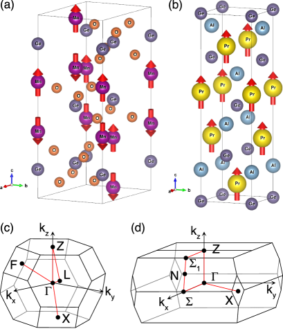
Figure 9: Crystal and magnetic structures of (a) MnGeO₃ and (b) PrGeAl. The associated Brillouin zones are shown in (c) and (d), respectively.

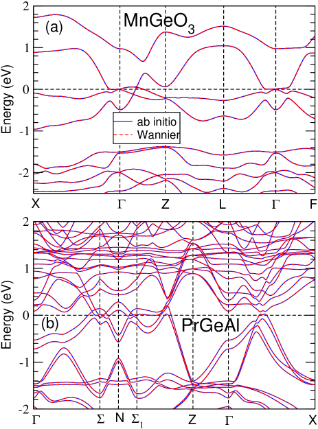
Figure 10: Fully-relativistic band structures of (a) antiferromagnetic MnGeO₃ and (b) ferromagnetic PrGeAl. The Fermi level ($E_{F}$) is at 0 eV.

The electronic band structure and magnetic properties of MnGeO₃ and PrGeAl are calculated based on first-principles density functional theory with the generalized gradient approximation (GGA) [70]. The experimental structural parameters for MnGeO₃ [67] and PrGeAl [69] are used in the present calculations. To better describe the Coulomb correlation among Mn 3$d$ electrons and also among Pr 4$f$ electrons, we adopt the GGA+$U$ scheme [71]. Following the recent studies [42, 43], we use the effective $U$ value of 4.0 eV for both Mn 3$d$ and Pr 4$f$ electrons. The calculations are performed using the accurate projector-augmented wave (PAW) method [72], as implemented in the Vienna ab-initio simulation package (VASP) [73, 74]. The fully relativistic PAW potentials are adopted in order to include the spin-orbit coupling (SOC) effect. Large plane-wave cutoff energies of 450 eV and 500 eV are used for MnGeO₃ and PrGeAl, respectively. For the Brillouin zone integration, $k$-point meshes of 12 $\times$ 12 $\times$ 12 and 16 $\times$ 16 $\times$ 16 are used for MnGeO₃ and PrGeAl, respectively. All the calculations are performed with an energy convergence within 10^-6 eV between the successive iterations.

Here we consider MnGeO₃ and PrGeAl, respectively, in the AF and FM states with the magnetic moments being parallel to the $c$-axis. The calculated relativistic band structures of MnGeO₃ and PrGeAl are displayed in Fig. 10(a) and Fig. 10(b), respectively. They are both semimetals with low density of states at the Fermi level ($E_{F}$) of 0.315 states/eV/f.u. and 0.133 states/eV/f.u., respectively. The calculated Mn spin magnetic moment in MnGeO₃ is 4.29 $\mu_{B}$ and that of Pr in PrGeAl is 1.89 $\mu_{B}$. The calculated band structures agree well with that reported previously [42, 43].

Nonlinear optical photocurrents are calculated based on the linear response formalism with the independent particle approximation, as described above. Specifically, the DC shift and injection photocurrent conductivity tensors are calculated using Eq. (4) given in Sec. II. Since a large number of $k$-points are needed to get accurate NLO responses [75, 76], we use the efficient Wannier function interpolation method based on maximally localized Wannier functions (MLWFs) [77, 78, 79]. For MnGeO₃, 68 MLWFs per unit cell of Mn $d$, Ge $p$ and O $p$ orbitals are constructed by fitting to the GGA+U+SOC band structure. In PrGeAl, 76 MLWFs per unit cell of Pr $d$ and $f$ orbitals as well as Ge $p$ and Al $sp$ orbitals are adopted. The band structures obtained by the Wannier interpolation are nearly identical to that from the GGA+U+SOC calculations (see Fig. 10). The shift current conductivity tensors are then evaluated by taking very dense $k$-point meshes of 200 $\times 200$ $\times$ 200 for MnGeO₃ and of 160 $\times 160$ $\times$ 220 for PrGeAl. We find that the conductivity tensors obtained using such dense $k$-point meshes converge within a few percent. Here we consider the ”cold” semimetals, i.e., the Fermi-Dirac function in Eq. (4) is taken to be a step function. Furthermore, the Dirac $\delta$ function is replaced by a Lorentzian function with broadenning width of $\hbar\tau^{-1}=10$ meV. Accordingly, in the injection conductivity calculations, we use the relaxation time $\tau$ given by $\hbar\tau^{-1}=10$ meV.

References

- Liu et al. [2020] J. Liu, F. Xia, D. Xiao, J. G. de Abajo, and D. Sun, Semimetals for high performance photodetection, Nat. Mater. 19, 830 (2020).
- Kraut and von Baltz [1979] W. Kraut and R. von Baltz, Anomalous bulk photovoltaic effect in ferroelectrics: a quadratic response theory, Physical Review B 19, 1548 (1979).
- von Baltz and Kraut [1981] R. von Baltz and W. Kraut, Theory of the bulk photovoltaic effect in pure crystals, Physical Review B 23, 5590 (1981).
- Morimoto and Nagaosa [2016] T. Morimoto and N. Nagaosa, Topological nature of nonlinear optical effects in solids, Sci. Adv. 2, e1501524 (2016).
- de Juan et al. [2017] F. de Juan, A. G. Grushin, T. Morimoto, and J. E. Moore, Quantized circular photogalvanic effect in Weyl semimetals, Nat. Commun. 8, 15995 (2017).
- Nagaosa and Morimoto [2017] N. Nagaosa and T. Morimoto, Concept of quantum geometry in optoelectronic processes in solids: Application to solar cells, Adv. Mater. 29, 1603345 (2017).
- Sipe and Shkrebtii [2000] J. E. Sipe and A. I. Shkrebtii, Second-order optical response in semiconductors, Phys. Rev. B 61, 5337 (2000).
- Morimoto et al. [2016] T. Morimoto, S. Zhong, J. Orenstein, and J. E. Moore, Semiclassical theory of nonlinear magneto-optical responses with applications to topological Dirac/Weyl semimetals, Phys. Rev. B 94, 245121 (2016).
- König et al. [2017] E. J. König, H.-Y. Xie, D. A. Pesin, and A. Levchenko, Photogalvanic effect in Weyl semimetals, Phys. Rev. B 96, 075123 (2017).
- Kim et al. [2017] K. W. Kim, T. Morimoto, and N. Nagaosa, Shift charge and spin photocurrents in Dirac surface states of topological insulator, Phys. Rev. B 95, 035134 (2017).
- Ma et al. [2017] Q. Ma, S.-Y. Xu, C.-K. Chan, C.-L. Zhang, G. Chang, Y. Lin, W. Xie, T. Palacios, H. Lin, S. Jia, et al., Direct optical detection of Weyl fermion chirality in a topological semimetal, Nat. Phys. 13, 842 (2017).
- Wu et al. [2017] L. Wu, S. Patankar, T. Morimoto, N. L. Nair, E. Thewalt, A. Little, J. G. Analytis, J. E. Moore, and J. Orenstein, Giant anisotropic nonlinear optical response in transition metal monopnictide Weyl semimetals, Nat. Phys. 13, 350 (2017).
- Yang et al. [2017] X. Yang, K. Burch, and Y. Ran, Divergent bulk photovoltaic effect in Weyl semimetals, arXiv:1712.09363 (2017).
- Golub and Ivchenko [2018] L. E. Golub and E. L. Ivchenko, Circular and magnetoinduced photocurrents in Weyl semimetals, Phys. Rev. B 98, 075305 (2018).
- Flicker et al. [2018] F. Flicker, F. de Juan, B. Bradlyn, T. Morimoto, M. G. Vergniory, and A. G. Grushin, Chiral optical response of multifold fermions, Phys. Rev. B 98, 155145 (2018).
- Zhang et al. [2018] Y. Zhang, H. Ishizuka, J. van den Brink, C. Felser, B. Yan, and N. Nagaosa, Photogalvanic effect in Weyl semimetals from first principles, Phys. Rev. B 97, 241118(R) (2018).
- Osterhoudt et al. [2019] G. B. Osterhoudt, L. K. Diebel, M. J. Gray, X. Yang, J. Stanco, X. Huang, B. Shen, N. Ni, P. J. W. Moll, Y. Ran, et al., Colossal mid-infrared bulk photovoltaic effect in a type-I Weyl semimetal, Nat. Mater. 18, 471 (2019).
- Ma et al. [2019] J. Ma, Q. Gu, Y. Liu, J. Lai, P. Yu, X. Zhuo, Z. Liu, J.-H. Chen, J. Feng, and D. Sun, Nonlinear photoresponse of type-II Weyl semimetals, Nat. Mater. 18, 476 (2019).
- Parker et al. [2019] D. E. Parker, T. Morimoto, J. Orenstein, and J. E. Moore, Diagrammatic approach to nonlinear optical response with application to Weyl semimetals, Phys. Rev. B 99, 045121 (2019).
- Young and Rappe [2012] S. M. Young and A. M. Rappe, First principles calculation of the shift current photovoltaic effect in ferroelectrics, Phys. Rev. Lett. 109, 116601 (2012).
- Fregoso et al. [2017] B. M. Fregoso, T. Morimoto, and J. E. Moore, Quantitative relationship between polarization differences and the zone-averaged shift photocurrent, Phys. Rev. B 96, 075421 (2017).
- Holder et al. [2020] T. Holder, D. Kaplan, and B. Yan, Consequences of time-reversal-symmetry breaking in the light-matter interaction: Berry curvature, quantum metric, and diabatic motion, Physical Review Research 2, 033100 (2020).
- Semenov et al. [2012] Y. G. Semenov, X. Li, and K. W. Kim, Tunable photogalvanic effect on topological insulator surfaces via proximity interactions, Phys. Rev. B 86, 201401(R) (2012).
- Ogawa et al. [2016] N. Ogawa, R. Yoshimi, K. Yasuda, A. Tsukazaki, M. Kawasaki, and Y. Tokura, Zero-bias photocurrent in ferromagnetic topological insulator, Nat. Commun. 7, 12246 (2016).
- Chan et al. [2017] C.-K. Chan, N. H. Lindner, G. Refael, and P. A. Lee, Photocurrents in Weyl semimetals, Phys. Rev. B 95, 041104(R) (2017).
- Zhang et al. [2019] Y. Zhang, T. Holder, H. Ishizuka, F. de Juan, N. Nagaosa, C. Felser, and B. Yan, Switchable magnetic bulk photovoltaic effect in the two-dimensional magnet CrI3, Nat. Commun. 10, 3783 (2019).
- Sun et al. [2019] Z. Sun, Y. Yi, T. Song, G. Clark, B. Huang, Y. Shan, S. Wu, D. Huang, C. Gao, Z. Chen, et al., Giant nonreciprocal second-harmonic generation from antiferromagnetic bilayer CrI3, Nature 572, 497 (2019).
- Mendis [1968] P. Mendis, Photocurrent in a semiconductor without a symmetry center, ZhETF Pisma Redaktsiiu 7, 355 (1968).
- Genkin and Mednis [1968] V. N. Genkin and P. M. Mednis, Contribution to the theory of nonlinear effects in crystals with account taken of partially filled bands, Sov. Phys. JETP 27, 609 (1968).
- Sturman and Fridkin [1992] B. I. Sturman and V. M. Fridkin, The Photovoltaic and Photo-refractive Effects in Noncentrosymmetric Materials, Vol. 8 (CRC Press, 1992).
- Liu et al. [2019] D. F. Liu, A. J. Liang, E. K. Liu, Q. N. Xu, Y. W. Li, C. Chen, D. Pei, W. J. Shi, S. K. Mo, P. Dudin, et al., Magnetic Weyl semimetal phase in a Kagomé crystal, Science 365, 1282 (2019).
- Belopolski et al. [2019] I. Belopolski, K. Manna, D. S. Sanchez, G. Chang, B. Ernst, J. Yin, S. S. Zhang, T. Cochran, N. Shumiya, H. Zheng, et al., Discovery of topological Weyl fermion lines and drumhead surface states in a room temperature magnet, Science 365, 1278 (2019).
- Morali et al. [2019] N. Morali, R. Batabyal, P. K. Nag, E. Liu, Q. Xu, Y. Sun, B. Yan, C. Felser, N. Avraham, and H. Beidenkopf, Fermi-arc diversity on surface terminations of the magnetic Weyl semimetal Co3Sn2S2, Science 365, 1286 (2019).
- Xu et al. [2011] G. Xu, H. Weng, Z. Wang, X. Dai, and Z. Fang, Chern semimetal and the quantized anomalous Hall effect in HgCr2Se4, Phys. Rev. Lett. 107, 186806 (2011).
- Hirschberger et al. [2016] M. Hirschberger, S. Kushwaha, Z. Wang, Q. Gibson, S. Liang, C. A. Belvin, B. A. Bernevig, R. J. Cava, and N. P. Ong, The chiral anomaly and thermopower of Weyl fermions in the half-heusler GdPtBi, Nat. Mater. 15, 1161 (2016).
- Kushwaha et al. [2018] S. K. Kushwaha, Z. Wang, T. Kong, and R. J. Cava, Magnetic and electronic properties of the Cu-substituted Weyl semimetal candidate ZrCo2Sn, J. Phys. Condens. 30, 075701 (2018).
- Zou et al. [2019] J. Zou, Z. He, and G. Xu, The study of magnetic topological semimetals by first principles calculations, npj Comput. Mater. 5, 96 (2019).
- Jin et al. [2019] H.-S. Jin, Y.-J. Song, W. E. Pickett, and K.-W. Lee, Noncentrosymmetric compensated half-metal hosting pure spin Weyl nodes, triple nodal points, nodal loops, and nexus fermions, Phys. Rev. Materials 3, 021201 (2019).
- Tang et al. [2016] P. Tang, Q. Zhou, G. Xu, and S.-C. Zhang, Dirac fermions in an antiferromagnetic semimetal, Nat. Phys. 12, 1100 (2016).
- Armitage et al. [2018] N. P. Armitage, E. J. Mele, and A. Vishwanath, Weyl and Dirac semimetals in three-dimensional solids, Reviews of Modern Physics 90, 015001 (2018).
- Lin et al. [2019] Z. Lin, C. Wang, P. Wang, S. Yi, L. Li, Q. Zhang, Y. Wang, Z. Wang, Y. Sun, Z. Sun, et al., Dirac fermions in antiferromagnetic fesn Kagomé lattices with combined space inversion and time reversal symmetry, arXiv:1906.05755 (2019).
- Xu et al. [2020] Y. Xu, L. Elcoro, Z. Song, B. J. Wieder, M. G. Vergniory, N. Regnault, Y. Chen, C. Felser, and B. A. Bernevig, High-throughput calculations of antiferromagnetic topological materials from magnetic topological quantum chemistry, arXiv:2003.00012 (2020).
- Chang et al. [2018] G. Chang, B. Singh, S.-Y. Xu, G. Bian, S.-M. Huang, C.-H. Hsu, I. Belopolski, N. Alidoust, D. S. Sanchez, H. Zheng, et al., Magnetic and noncentrosymmetric weyl fermion semimetals in the r alge family of compounds (r= rare earth), Physical Review B 97, 041104(R) (2018).
- Sanchez et al. [2020] D. S. Sanchez, G. Chang, I. Belopolski, H. Lu, J.-X. Yin, N. Alidoust, X. Xu, T. A. Cochran, X. Zhang, Y. Bian, et al., Observation of weyl fermions in a magnetic non-centrosymmetric crystal, Nature communications 11, 1 (2020).
- Bhalla et al. [2020] P. Bhalla, A. H. MacDonald, and D. Culcer, Resonant photovoltaic effect in doped magnetic semiconductors, Physical Review Letters 124, 087402 (2020).
- Aversa and Sipe [1995] C. Aversa and J. E. Sipe, Nonlinear optical susceptibilities of semiconductors: Results with a length-gauge analysis, Physical Review B 52, 14636 (1995).
- de Juan et al. [2020] F. de Juan, Y. Zhang, T. Morimoto, Y. Sun, J. E. Moore, and A. G. Grushin, Difference frequency generation in topological semimetals, Phys. Rev. Research 2, 012017 (2020).
- Onsager [1931] L. Onsager, Reciprocal relations in irreversible processes. I., Phys. Rev. 37, 405 (1931).
- Kubo [1957] R. Kubo, Statistical-mechanical theory of irreversible processes. i. general theory and simple applications to magnetic and conduction problems, J. Phys. Soc. Japan 12, 570 (1957).
- Tokura and Nagaosa [2018] Y. Tokura and N. Nagaosa, Nonreciprocal responses from non-centrosymmetric quantum materials, Nat. Commun. 9, 3740 (2018).
- Gallego et al. [2019] S. V. Gallego, J. Etxebarria, L. Elcoro, E. S. Tasci, and J. M. Perez-Mato, Automatic calculation of symmetry-adapted tensors in magnetic and non-magnetic materials: a new tool of the bilbao crystallographic server, Acta Crystallogr. A 75, 438 (2019).
- Yang and Nagaosa [2014] B.-J. Yang and N. Nagaosa, Classification of stable three-dimensional Dirac semimetals with nontrivial topology, Nat. Commun. 5, 4898 (2014).
- Nielsen and Ninomiya [1981] H. B. Nielsen and M. Ninomiya, No-go theorem for regularizing chiral fermions, Tech. Rep. 2-3 (1981).
- Witten [2016] E. Witten, Three lectures on topological phases of matter, Riv. del Nuovo Cim. 39, 313 (2016).
- Soluyanov et al. [2015] A. A. Soluyanov, D. Gresch, Z. Wang, Q. Wu, M. Troyer, X. Dai, and B. A. Bernevig, Type-II Weyl semimetals, Nature 527, 495 (2015).
- Provost and Vallee [1980] J. P. Provost and G. Vallee, Riemannian structure on manifolds of quantum states, Communications in Mathematical Physics 76, 289 (1980).
- Cook et al. [2017] A. M. Cook, B. M. Fregoso, F. de Juan, S. Coh, and J. E. Moore, Design principles for shift current photovoltaics, Nat. Commun. 8, 14176 (2017).
- Kolodrubetz et al. [2017] M. Kolodrubetz, D. Sels, P. Mehta, and A. Polkovnikov, Geometry and non-adiabatic response in quantum and classical systems, Phys. Rep. 697, 1 (2017).
- Gelfand et al. [1997] I. Gelfand, V. Retakh, and M. Shubin, Fedosov manifolds, arXiv:dg-ga/9707024 (1997).
- Nakahara [2003] M. Nakahara, Geometry, Topology and Physics (CRC Press, 2003).
- Sodemann and Fu [2015] I. Sodemann and L. Fu, Quantum nonlinear Hall effect induced by Berry curvature dipole in time-reversal invariant materials, Phys. Rev. Lett. 115, 216806 (2015).
- Gao and Xiao [2019] Y. Gao and D. Xiao, Nonreciprocal directional dichroism induced by the quantum metric dipole, Phys. Rev. Lett. 122, 227402 (2019).
- Rezakhani et al. [2010] A. T. Rezakhani, D. F. Abasto, D. A. Lidar, and P. Zanardi, Intrinsic geometry of quantum adiabatic evolution and quantum phase transitions, Phys. Rev. A 82, 012321 (2010).
- Ma et al. [2010] Y.-Q. Ma, S. Chen, H. Fan, W.-M. Liu, et al., Abelian and non-abelian quantum geometric tensor, Phys. Rev. B 81, 245129 (2010).
- Wang et al. [2012] Z. Wang, Y. Sun, X.-Q. Chen, C. Franchini, G. Xu, H. Weng, X. Dai, and Z. Fang, Dirac semimetal and topological phase transitions in A3Bi (A= Na, K, Rb), Phys. Rev. B 85, 195320 (2012).
- Wang et al. [2013] Z. Wang, H. Weng, Q. Wu, X. Dai, and Z. Fang, Three-dimensional Dirac semimetal and quantum transport in Cd3As2, Phys. Rev. B 88, 125427 (2013).
- Tsuzuki et al. [1974] K. Tsuzuki, Y. Ishikawa, N. Watanabe, and S. Akimoto, Neutron diffraction and paramagnetic scattering from a high pressure phase of mngeo3 (ilmenite), Journal of the Physical Society of Japan 37, 1242 (1974).
- Nastos and Sipe [2010] F. Nastos and J. E. Sipe, Optical rectification and current injection in unbiased semiconductors, Physical Review B 82, 235204 (2010).
- Gladyshevskii et al. [2000] E. Gladyshevskii, N. Nakonechna, K. Cenzual, R. Gladyshevskii, and J.-L. Jorda, Crystal structures of pralxge2- x compounds, Journal of alloys and compounds 296, 265 (2000).
- Perdew et al. [1996] J. P. Perdew, K. Burke, and M. Ernzerhof, Generalized gradient approximation made simple, Physical review letters 77, 3865 (1996).
- Dudarev et al. [1998] S. L. Dudarev, G. A. Botton, S. Y. Savrasov, C. J. Humphreys, and A. P. Sutton, Electron-energy-loss spectra and the structural stability of nickel oxide: An lsda+ u study, Physical Review B 57, 1505 (1998).
- Blöchl [1994] P. E. Blöchl, Projector augmented-wave method, Physical review B 50, 17953 (1994).
- Kresse and Hafner [1993] G. Kresse and J. Hafner, Ab initio molecular dynamics for liquid metals, Physical Review B 47, 558 (1993).
- Kresse and Furthmüller [1996] G. Kresse and J. Furthmüller, Efficient iterative schemes for ab initio total-energy calculations using a plane-wave basis set, Physical review B 54, 11169 (1996).
- Guo et al. [2004] G. Y. Guo, K. C. Chu, D. S. Wang, and C. G. Duan, Linear and nonlinear optical properties of carbon nanotubes from first-principles calculations, Physical Review B 69, 205416 (2004).
- Wang and Guo [2015] C.-Y. Wang and G.-Y. Guo, Nonlinear optical properties of transition-metal dichalcogenide mx2 (m= mo, w; x= s, se) monolayers and trilayers from first-principles calculations, The Journal of Physical Chemistry C 119, 13268 (2015).
- Wang et al. [2006] X. Wang, J. R. Yates, I. Souza, and D. Vanderbilt, Ab initio calculation of the anomalous hall conductivity by wannier interpolation, Physical Review B 74, 195118 (2006).
- Marzari et al. [2012] N. Marzari, A. A. Mostofi, J. R. Yates, I. Souza, and D. Vanderbilt, Maximally localized wannier functions: Theory and applications, Reviews of Modern Physics 84, 1419 (2012).
- Ibañez-Azpiroz et al. [2018] J. Ibañez-Azpiroz, S. S. Tsirkin, and I. Souza, Ab initio calculation of the shift photocurrent by wannier interpolation, Physical Review B 97, 245143 (2018).