Diffuse Ionized Gas in Simulations of Multiphase, Star-Forming Galactic Disks

Abstract

It has been hypothesized that photons from young, massive star clusters are responsible for maintaining the ionization of diffuse warm ionized gas seen in both the Milky Way and other disk galaxies. For a theoretical investigation of the warm ionized medium (WIM), it is crucial to solve radiation transfer equations where the ISM and clusters are modeled self-consistently. To this end, we employ a Solar neighborhood model of TIGRESS, a magnetohydrodynamic simulation of the multiphase, star-forming ISM, and post-process the simulation with an adaptive ray tracing method to transfer UV radiation from star clusters. We find that the WIM volume filling factor is highly variable, and sensitive to the rate of ionizing photon production and ISM structure. The mean WIM volume filling factor rises to $\sim 0.15$ at $|z|\sim 1\,{\rm kpc}$. Approximately half of ionizing photons are absorbed by gas and half by dust; the cumulative ionizing photon escape fraction is 1.1%. Our time-averaged synthetic ${\rm H}\alpha$ line profile matches WHAM observations on the redshifted (outflowing) side, but has insufficient intensity on the blueshifted side. Our simulation matches the Dickey-Lockman neutral density profile well, but only a small fraction of snapshots have high-altitude WIM density consistent with Reynolds Layer estimates. We compute a clumping correction factor $\mathcal{C}_{n_{e}}\equiv\langle n_{e}\rangle/\langle n_{e}^{2}\rangle^{1/2}\sim 0.2$ that is remarkably constant with distance from the midplane and time; this can be used to improve estimates of ionized gas mass and mean electron density from observed ${\rm H}\alpha$ surface brightness profiles in edge-on galaxies.

1 Introduction

The presence of a diffuse layer of ionized gas reaching over $1\,{\rm kpc}$ above the Galactic plane has been known for decades (Hoyle & Ellis, 1963; Reynolds et al., 1973), and the physical properties of this diffuse warm ionized medium (WIM) have been characterized based on a variety of observational diagnostics (e.g., Reynolds, 1989, 1991b; Madsen et al., 2006; Gaensler et al., 2008; Hill et al., 2008). Wide field ${\rm H}\alpha$ surveys have in particular expanded the view of the WIM to the full sky (Haffner et al., 2003, 2010). Beyond the Milky Way, analogous distributions of diffuse ionized gas (DIG) have been seen in many nearby disk galaxies (e.g., Rand et al., 1990; Dettmar, 1990; Zurita et al., 2000; Jones et al., 2017; Jo et al., 2018; Levy et al., 2019). Haffner et al. (2009) reviews both Galactic and extragalactic observations, and adopts the convention of using “WIM” for the Milky Way and “DIG” for other galaxies to indicate a diffuse component of warm ionized gas. In this work, we use “WIM” or “warm ionized gas” to refer to any photoionized gas in simulations, and apply the term “DIG” to the diffuse portion at high altitude regions. When referring to observations, we also use the term “WIM” for generic ionized gas if the context is clear.

Observations of optical line emission ratios suggest that the temperature of the WIM ranges from $6000\,{\rm K}$ to $10000\,{\rm K}$, slightly higher than that of classical H II regions (e.g., Madsen et al., 2006). The dispersion measure (${\rm DM}=\int n_{\rm e}d\ell$) of pulsars with known distances shows that the line-of-sight averaged free electron density is $\sim 0.01$–$0.1\,{\rm cm}^{-3}$, with a vertical exponential scale height of $h(n_{\rm e})\sim 1\,{\rm kpc}$ (e.g., Reynolds 1991a; Nordgren et al. 1992; Gómez et al. 2001; Gaensler et al. 2008; Deller et al. 2019; see also Savage et al. 1990; Peterson & Webber 2002; Savage & Wakker 2009, which estimated the scale height via other means). Studies combining measurements of the emission measure (${\rm EM}=\int n_{\rm e}^{2}d\ell$; typically derived from ${\rm H}\alpha$ surface brightness) and the DM suggest that the volume filling fraction of WIM is $\lesssim 0.1$ at the midplane and $\sim 0.2$–$0.4$ at $|z|\sim 1\,{\rm kpc}$ (e.g., Reynolds, 1991b; Berkhuijsen et al., 2006; Gaensler et al., 2008). The Milky Way EM scale height (obtained by fitting an exponential to the ${\rm H}\alpha$ intensity as a function of height from the midplane) is smaller ($\sim 250$–$550\,{\rm pc}$; Haffner et al. 1999; Hill et al. 2014; Krishnarao et al. 2017), although an anomalously high value ($>1\,{\rm kpc}$) has been found along the far Carina arm (Krishnarao et al., 2017). The ${\rm H}\alpha$ scale heights of external (edge-on) galaxies range from a few hundred pc to over $2\,{\rm kpc}$ (e.g., Jo et al., 2018; Boettcher et al., 2019; Levy et al., 2019). In both the Milky Way and other nearby galaxies, the distribution of diffuse ${\rm H}\alpha$ surface brightness (projected on the disk plane) is well characterized by a lognormal (Hill et al., 2008; Seon, 2009; Berkhuijsen & Fletcher, 2015).

The mechanism for maintaining warm ionized gas far from the midplane has been debated since its discovery. Proposed mechanisms for the origin of extraplanar warm gas include the cooling of hot galactic fountain gas (Shapiro & Field, 1976; Bregman, 1980), gas accretion from the intergalactic medium (Binney, 2005), and entrainment of warm ISM clouds by hot winds. Based on analysis of flows in numerical simulations with clustered supernovae, Kim et al. (2017a) and Kim & Ostriker (2018) showed that significant amounts of warm gas are accelerated by superbubble expansion, producing an exponential distribution of velocities. This high-velocity warm gas, with speeds up to $\sim 100\,{\rm km}\,{\rm s}^{-1}$, creates a fountain in the extraplanar regions if the halo potential is too deep for the gas to escape (see also Fielding et al., 2018; Vijayan et al., 2019).

Regardless of the mechanism for populating high-altitude regions with warm gas, photoionization from young, massive stars in the disk has long been thought to be the dominant mechanism that ionizes the Milky Way’s DIG (Bregman & Harrington, 1986; Reynolds, 1990; Dove & Shull, 1994; Miller & Cox, 1993; Reynolds et al., 1995).

Indeed, past numerical work has shown that photoionization from O and B stars is capable of ionizing diffuse gas far from the midplane, if such a diffuse gas layer is present and if there are a sufficient number of low density paths in the intervening material through which ionizing photons may propagate. For example, based on Monte-Carlo photoionization post-processing of the turbulent hydrodynamic simulations of Joung & Mac Low (2006), Wood et al. (2010) showed that ionizing photons are able to travel large ($\sim{\rm kpc}$) distances from the midplane and produce a layer of ionized gas with exponential scale height of $n_{\rm e}$ of $500\,{\rm pc}$. Wood et al. (2010) also found that the ionizing photon rate has a strong influence on the extent and vertical profile of WIM. Similarly, Barnes et al. (2014) post-processed the magnetohydrodynamic (MHD) simulations of Hill et al. (2012), finding that the additional pressure support from magnetic fields does not significantly change the high-altitude DIG. An exponential ${\rm H}\alpha$ scale height above $500\,{\rm pc}$ was found to be $\sim 150\,{\rm pc}$ and $250\,{\rm pc}$ for ionizing luminosity per source of $10^{50}\,{\rm s}^{-1}$ and $10^{49}\,{\rm s}^{-1}$, respectively; this is insufficient to match the observed extended ionized gas in the Milky Way. Vandenbroucke et al. (2018) repeated the analysis of Barnes et al. (2014) for snapshots from the SILCC simulation of Girichidis et al. (2016), and found that the exponential scale height of ${\rm H}\alpha$ reached $\sim 600-700\,{\rm pc}$ if cosmic rays are included, consistent with the observed scale heights of DIG in the Milky Way. However, when strong dynamical feedback from supernovae (or cosmic rays) is absent, as in the radiation hydrodynamic simulations of Vandenbroucke & Wood (2019) that included photoionization feedback alone, a DIG layer at high altitude that reproduces the observations cannot be sustained. In addition to the above studies, there are a few recent numerical simulations that have included the effect of time dependent ionizing radiation feedback in ISM disk models with self-consistent star formation (Peters et al., 2017; Kannan et al., 2020). However, these simulations have been run for at most 150 Myr (and are thus have not necessarily reached a statistically quasi-steady state), and have largely focused on the effect of early stellar feedback on star formation efficiency and near-midplane structure.

Massive stars play several roles in the maintenance of the DIG: they provide the ionizing radiation, and, as supernovae, create the hot and warm outflows that populate extraplanar regions, while also creating the pathways that allow ionizing photons to travel far from the midplane. Low density paths from the major ionizing sources near the midplane are present because the hot portion of the multiphase ISM (created in supernova shocks) fills a large fraction of the volume near the midplane (McKee & Ostriker, 1977; McCray & Snow, 1979), and because the warm and cold portions of the ISM are further clumped as a result of turbulence (which itself is a result of supernova remnant expansion).

The detailed structure of the multiphase ISM is quite sensitive to the spatio-temporal distribution of supernovae and their correlation with gas (Kim & Ostriker, 2018). However, previous simulations of the ISM that have been used as inputs to radiative transfer models of the WIM (e.g. Joung & Mac Low, 2006; Hill et al., 2012; Girichidis et al., 2016) lack self-consistency in modeling massive stars and supernovae. The spatial distribution and rate of supernovae are imposed “by hand” for dynamical modeling of the ISM, and the position and luminosity of ionizing radiation sources are imposed “by hand” for radiation post-processing. Imposing SN distributions by hand may affect the production of high-velocity warm outflows that is responsible for extraplanar gas. In addition, unrealistic SN distributions may strongly affect the ability of ionizing photons to propagate long distances through the ISM. For example, numerical simulations show that if supernova locations are entirely random, the resultant hot volume filling factor is much higher than if all supernovae explode in dense gas (Walch et al., 2015). Similarly, non-self-consistent locations of radiation sources with respect to the gas distribution will also affect photon propagation.

Because of the multiple roles that massive stars play in shaping the structure of the ISM, and the sensitivity of large-scale ISM structure and dynamics to the spatial correlation between SNe and gas, it is crucial to model the formation and destruction of massive stars self-consistently when studying formation of the DIG. To study gas properties in the extraplanar region, it is also crucial to achieve uniformly high spatial resolution so that (1) the majority of SN events are initiated in either the free-expansion or energy-conserving stage and hot gas is well-resolved when created by shocks, and (2) the interaction at high altitude between hot winds and warm fountain flows driven by clustered SNe is properly captured (Kim & Ostriker, 2018; Vijayan et al., 2019).

In this work, we use adaptive ray tracing to propagate photons through an MHD simulation of the star-forming ISM, and investigate the properties of the resultant WIM. The approach we use is to post-process snapshots from a model representative of conditions in the Solar neighborhood, produced within the Three-phase Interstellar Medium in Galaxies Resolving Evolution with Star Formation and Supernova Feedback (hereafter TIGRESS) framework (Kim & Ostriker, 2017). The TIGRESS framework simulates local patches of a galactic disk at uniformly high resolution, including effects of magnetic fields, galactic sheared rotation, self-gravity, and feedback in the form of FUV heating and supernovae. In the TIGRESS framework, star cluster formation via local gravitational collapse and feedback from supernovae are modeled self-consistently. The distribution of stellar energy sources within the multiphase ISM structure in the self-consistent TIGRESS framework presumably yields realistic space-time correlations of radiation sources and absorption sites.

The layout of the paper is as follows. In Section 2, we provide details of the underlying TIGRESS model and the adaptive ray tracing method used to track UV radiation from massive stars. In Section 3, we review the overall time evolution of the post-processed simulation, the resulting density structure and statistical properties of the warm ionized gas (including gas/dust absorption and escape fractions of radiation), and construct spatially integrated ${\rm H}\alpha$ line profiles. In Section 4, we first compare our study with previous numerical work on formation of the WIM, and then discuss observational applications of our results. Here, we compare our derived scale heights to observations of both the Milky Way and external galaxies, and describe our calibration of a clumping correction factor which will allow for observations of the EM in edge-on galaxies to be converted to a mean electron density along the line of sight.

2 Methods

In this section, we describe the MHD simulation used for modeling the star-forming galactic disk and our procedure for post-processing simulation snapshots with adaptive ray tracing to compute radiation energy densities and equilibrium ionization fractions.

2.1 MHD Simulation

The TIGRESS framework is built on the grid-based MHD code Athena (Stone et al., 2008), with additional physics modules for shearing box boundary conditions (Stone & Gardiner, 2010), self-gravity, sink/star particles, and star formation feedback in the form of clustered and distributed supernovae and optically thin heating and cooling. Kim & Ostriker (2017) present full details of physical processes modeled and their implementation, results for basic physical properties of the fiducial Solar neighborhood model, and a numerical convergence study. Here, we give a brief overview of the numerical methods for star cluster formation and stellar feedback employed in the TIGRESS framework.

To model the formation of star clusters and their feedback, the TIGRESS framework employs the sink particle module of Gong & Ostriker (2013), with some updates. A sink particle, representing a star cluster, is created if the gas in a cell (1) exceeds the Larson-Penston density threshold at local gas sound speed, (2) is at a local minimum of the gravitational potential, and (3) has a converging velocity field in all three directions. The particles’ equation of motion is integrated by a symplectic orbit integration scheme of (Quinn et al., 2010) in the shearing box frame under the total (gas, external, and particle) gravitational potential. The sink particles accrete mass fluxes into a virtual control volume ($3^{3}$ cells surrounding a particle) if gas flows are converging from all three directions in the particle’s rest frame. At the time of particle formation and whenever a given particle is accreting gas, its control volume is reset with the extrapolated density, momentum, and energy from the nearby cells, and only the difference between original and extrapolated values of mass and momentum is dumped into the sink particle. Sink particles accrete and merge only before the advent of supernovae.

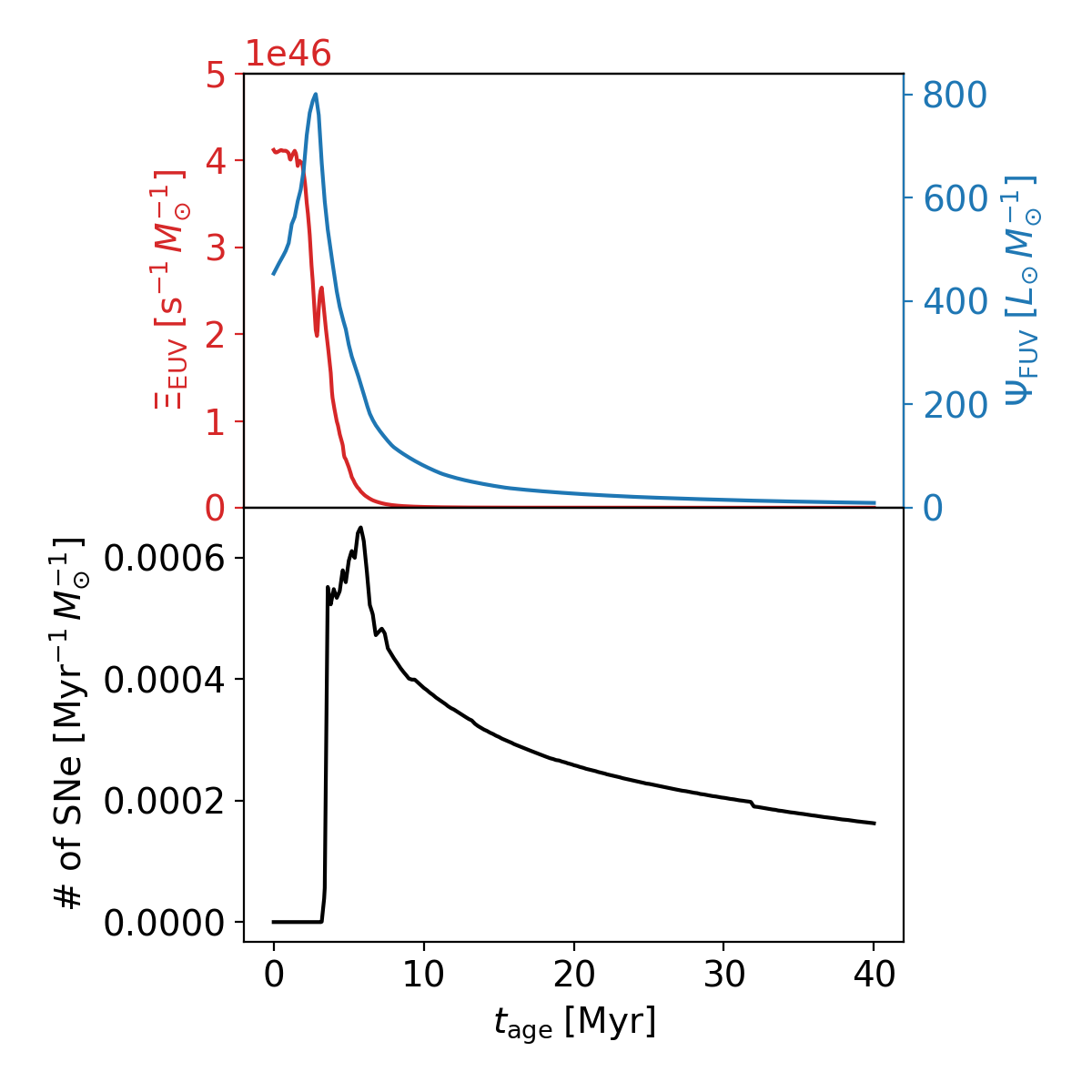
Figure 1: Top: Specific FUV luminosity $\Psi_{\rm FUV}$ (blue) and specific ionizing photon rate $\Xi_{\rm EUV}$ (red); Bottom: Specific SNe rate. Rates are shown as functions of the age of a star cluster that fully samples the Kroupa initial mass function (IMF). Calculated from STARBURST99.

TIGRESS incorporates stellar feedback from young stars in the form of clustered/distributed SNe as well as FUV radiation. Each star cluster particle in the simulation represents a star cluster with coeval stellar population that fully samples the Kroupa initial mass function (IMF) (Kroupa, 2001) with mass-weighted mean age $t_{\rm sp}$. All star cluster particles with $t_{\rm sp}<40\,{\rm Myr}$ can provide stellar feedback. Depending on the local density of the ambient medium and/or spatial resolution where a SN event occurs, SN feedback is implemented by either (1) direct injection of high-velocity SN ejecta (free-expansion stage), (2) injection of thermal + kinetic energy (energy-conserving, Sedov-Taylor stage), or (3) momentum (momentum-conserving stage). This ensures that the final radial momentum added to the surrounding ISM is consistent with the results from simulations of resolved SN remnant evolution (see Kim & Ostriker, 2015, and references therein).

The specific FUV luminosity $\Psi_{\rm FUV}$ and SN rate $\xi_{\rm SN}$ of individual star particles are determined from the STARBURST99 population synthesis model (adopting Geneva tracks with zero rotation, Pauldrich model atmosphere, and solar metallicity; Leitherer et al., 1999). The blue curve in the top panel of Figure 1 shows $\Psi_{\rm FUV}\equiv L_{*}/M_{*}$ of coeval stellar populations sampling the Kroupa IMF, calculated from STARBURST99.

The clustered SNe occur at the positions of star particles with age $t_{\rm sp}\gtrsim 3.5\,{\rm Myr}$ (bottom panel of Figure 1), while the distributed SNe are modeled via runaway OB star particles that are ejected from star cluster particles with an ejection velocity distribution consistent with a binary population synthesis model (Eldridge et al., 2011). The clustered and distributed SNe constitute 2/3 and 1/3 of the total SNe events, respectively.

The heating for cold and warm gas ($T<2\times 10^{4}\,{\rm K}$, see Table 1) represents dust photoelectric heating caused by FUV photons (Wolfire et al., 1995). The local FUV intensity is assumed to be proportional to the total FUV luminosity of feedback particles (with a correction for dust shielding expected for a plane-parallel slab as described in Ostriker et al. 2010), but is spatially uniform across the simulation domain. An optically-thin cooling function following Koyama & Inutsuka (2002) is adopted for cold and warm gas ($T\lesssim 10^{4.2}\,{\rm K}$) and that of Sutherland & Dopita (1993) is used for hot gas under the assumption of collisional ionization equilibrium.

Table 1: Temperature boundaries for thermal phases

Phase	Temperature boundary
Cold	$T<184\,{\rm K}$
Unstable	$184\,{\rm K}<T<5050\,{\rm K}$
Warm	$5050\,{\rm K}<T<2\times 10^{4}\,{\rm K}$
Hot	$T>2\times 10^{4}\,{\rm K}$

We use the Solar neighborhood model (R8) presented in Kim et al. (2020, in prep), which adopts the same galactic conditions analyzed in Kim & Ostriker (2017), Kim & Ostriker (2018), and Vijayan et al. (2019), with additional updates for the treatment of sink particle accretion as described above. We adopt the galactocentric distance $R_{0}=8\,{\rm kpc}$, angular velocity of local galactic rotation $\Omega=28\,{\rm km}\,{\rm s}^{-1}\,{\rm kpc}^{-1}$, and shear parameter $d\ln\Omega/d\ln R=-1$. The initial gas surface density is $\Sigma_{0}=13\,M_{\odot}\,{\rm pc}^{-2}$. The total gas mass decreases gradually as gas turns into stars and outflows escape the vertical boundaries. The box size for this model is $L_{x}=L_{y}=1024\,{\rm pc}$ and $L_{z}=7168\,{\rm pc}$ with a uniform grid spacing $\Delta x=4\,{\rm pc}$. The simulation is run for $660\,{\rm Myr}$ (3 orbital times), long enough for the system to establish a statistically quasi-steady state in which the physical state of the multiphase, turbulent ISM is consistently generated from star formation and supernova plus heating feedback. The impact of the initial transient evolution is minimal after $\sim 100\,{\rm Myr}$. Full data output snapshots are taken at intervals of $0.97\,{\rm Myr}(=1\,{\rm pc}/(1\,{\rm km}\,{\rm s}^{-1}))$.

2.2 Post-processing with Adaptive Ray Tracing

The MHD simulation snapshots are post-processed with the adaptive ray tracing algorithm implemented in the Athena code by Kim et al. (2017b), which solves the equation of radiative transfer for systems containing multiple point sources (neglecting scattering). For each snapshot, we read in the hydrogen number density ($n_{\rm H}$) and temperature ($T$) of gas, star particle data (position, mass, age for each source), and the simulation time ($t$) as inputs.

For a sink particle of mass $M_{\rm sp}$ and mass-weighted mean age $t_{\rm sp}(<40\,{\rm Myr})$, we calculate the ionizing photon production rate as $Q_{\rm i,sp}=\Xi_{\rm EUV}(t_{\rm sp})M_{\rm sp}$, where $\Xi_{\rm EUV}$ is the ionizing photon production rate per unit stellar mass (red line in Figure 1(a)). Because massive stars with lifetimes of $\sim 3\,{\rm Myr}$ dominate the ionizing photon output, $\Xi_{\rm i}$ is roughly constant at $4\times 10^{46}\,{\rm s}^{-1}\,M_{\odot}^{-1}$ before the onset of the first SN ($t_{\rm sp}\lesssim 3.5\,{\rm Myr}$), and declines sharply afterwards. Similarly, the FUV luminosity of each star particle is calculated as $L_{\rm FUV,sp}=\Psi_{\rm FUV}(t_{\rm sp})M_{\rm sp}$.

The adaptive ray tracing injects photon packets at the position of each sink particle and carries them along rays, calculating the local optical depth, the corresponding photon absorption rate by gas and dust, and the radiation energy density in two frequency bins (EUV and FUV). The ray direction is determined using the HEALPix scheme (Górski et al., 2005), which subdivides the unit sphere into $12\times 4^{\ell}$ equal-area pixels at HEALPix level $\ell$. We adopt the initial HEALPix level $\ell_{0}=4$ for the injected photon packets. Rays are split to ensure that each grid cell is sampled by at least four rays per source (unless one of the termination conditions is met; see below).

Similar to other flow attributes, the shearing-periodic boundary conditions are applied to rays crossing the radial ($x$) boundaries. For example, if a ray exits the far radial boundary at $y=y_{0}$, it re-enters the near radial boundary at $y=y_{0}+{\rm sgn}(L_{y}-\Delta y-y_{0})\times(L_{y}-\Delta y)$, where $\Delta y=(q\Omega L_{x}t\mod L_{y})$ is the shear displacement in the $y$-direction, with the position of the source offset accordingly. The azimuthal ($y$) boundary condition is strictly periodic.

Each photon packet is followed along a ray until one of the following conditions is satisfied: (1) the ray needs to split; (2) the optical depth from the source is greater than 10; (3) the ray exits the computational domain in the $d_{\rm xy}$ is greater than $d_{\rm xy,\rm max}=L_{x}=1024\,{\rm pc}$. Without the last condition, a small fraction of photon packets traveling a very long distance ($\gg L_{x}$) on horizontal optically-thin rays make the computational cost of ray tracing expensive. We have checked that the use of larger $d_{\rm xy,\rm max}$ has little impact on the outcome of our analysis.

For the opacity per unit length, we take $\chi_{\rm i}=n_{\rm H^{0}}\sigma_{\rm ph}+n_{\rm H}\sigma_{\rm d,i}$ and $\chi_{\rm n}=n_{\rm H}\sigma_{\rm d,n}$ for ionizing and non-ionizing radiation, respectively, where $\sigma_{\rm ph}=2.7\times 10^{-18}\,{\rm cm}^{2}\,{\rm H}^{-1}$ is the frequency-averaged photoionization cross section and $\sigma_{\rm d,i}=\sigma_{\rm d,n}=1.17\times 10^{-21}\,{\rm cm}^{2}\,{\rm H}^{-1}$ is the frequency-averaged dust absorption cross section (e.g., Draine, 2011a).

2.3 Runaways

In the TIGRESS framework, the age and orbits of runaway star particles are tracked consistently, and the ionizing photon rate of individual runaway star particles can be inferred from the total SN rate (bottom panel in Figure 1) and mass-luminosity relation for main-sequence stars (Parravano et al., 2003). To examine the effect of runaways on the ionization of gas, we post-processed the simulation snapshots including both clusters and runaway particles as ionizing sources. We find that including runaways does not change the extent and distribution of WIM significantly, because they contribute insignificantly to the total ionizing photon budget; the details of this calculation are summarized in Appendix A.

2.4 Ionization State Calculation

After the completion of a ray trace, we calculate the ionization state of a gas cell assuming simple ionization-recombination balance $\mathcal{I}_{\rm phot}+\mathcal{I}_{\rm coll}=\mathcal{R}$, where

$$\mathcal{I}_{\rm phot} =n_{\rm H^{0}}\sigma_{\rm ph}c\mathcal{E}_{\rm i}/(h\nu_{\rm i})$$ (1)

$$\mathcal{I}_{\rm coll} =\gamma_{\rm coll}n_{\rm H^{0}}n_{\rm e}$$ (2)

$$\mathcal{R} =\alpha_{\rm B}n_{\rm H^{+}}n_{\rm e}$$ (3)

are the local photoionization, collisional ionization, and radiative recombination rates, respectively. Here, $\mathcal{E}_{\rm i}$ is the radiation energy density for ionizing radiation, $h\nu_{\rm i}=18{\,{\rm eV}}$ the mean energy of ionizing photons, $\alpha_{\rm B}=2.59\times 10^{-13}(T/10^{4}\,{\rm K})^{-0.7}\,{\rm cm}^{3}\,{\rm s}^{-1}$ the case B recombination coefficient (Krumholz et al., 2007), $\gamma_{\rm coll}=5.84\times 10^{-11}\sqrt{T/{\rm K}}\exp({{-157821\,{\rm K}}/{T}})\,{\rm cm}^{3}\,{\rm s}^{-1}$ the collisional ionization rate coefficient (Tenorio-Tagle et al., 1986), $c$ the speed of light, $x_{\rm n}=n_{\rm H^{0}}/n_{\rm H}$ the neutral fraction, and $n_{\rm e}=n_{\rm H^{+}}=(1-x_{\rm n})n_{\rm H}$ the free electron number density. Note that for simplicity, we neglect the ionization of helium and other species, and free electrons released by them. Solving for $x_{\rm n}$ gives the equilibrium neutral fraction as

$$x_{\rm n}=\dfrac{2\alpha_{\rm B}n_{\rm H}}{(\Gamma+(2\alpha_{\rm B}+\gamma_{\rm coll})n_{\rm H})+\sqrt{(\Gamma+\gamma_{\rm coll}n_{\rm H})^{2}+4\Gamma\alpha_{\rm B}n_{\rm H}}}\,,$$ (4)

where $\Gamma=\mathcal{I}/n_{\rm H^{0}}$ (e.g., Altay & Theuns, 2013). In the absence of photoionization ($\Gamma=0)$, $x_{\rm n,coll}=\alpha_{\rm B}/(\alpha_{\rm B}+\gamma_{\rm coll})$.

In addition to the ionization balance, we assume that the thermal balance between heating and cooling keeps the temperature of photoionized gas at a constant value $T_{\rm ion}=10^{4}\,{\rm K}$. We alter the temperature of gas cells exposed to ionizing radiation as $T=T_{\rm ion}-(T_{\rm ion}-T_{0}){x_{\rm n,eq}}/{(2.0-x_{\rm n,eq})}$ if $T_{0}<T_{\rm ion}$, where $T_{0}$ is the temperature of gas in the MHD simulation. By doing so, the temperature of (collisionally ionized) hot gas remains unchanged, and the temperature of photoionized gas becomes $T\approx T_{\rm ion}=10^{4}\,{\rm K}$.

Since the change in gas temperature affects the recombination rate and the Strömgren volume calculation, the whole procedure (ray trace + equilibrium neutral fraction) is repeated until (1) the total volume of ionized gas converges to within $0.01\%$, and (2) the total ionization rate balances the recombination rate to within $0.01\%$. Each snapshot requires 20–30 iterations to converge to the desired accuracy.

We divide gas into four different phases based on temperature: $T>2\times 10^{4}\,{\rm K}$ for hot, $5050\,{\rm K}<T<2\times 10^{4}\,{\rm K}$ for warm, $184\,{\rm K}<T<5050\,{\rm K}$ for unstable, and $T\leq 184\,{\rm K}$ for cold (see Table 1). As noted in Section 1, we use “warm ionized gas” (or WIM) as a generic term to refer to both dense and diffuse photoionized gas in the simulation, and do not make a strict distinction between dense ionized gas (at low altitudes) and low-density ionized gas (both at low- and high-altitudes) since the dynamical expansion of “classical H II regions” is not modeled in the MHD simulation. Instead, we characterize the properties of warm ionized gas at varying densities and distance from the midplane , defined as $z=0$,. For practical purposes, we adopt $|z|=200\,{\rm pc}$ as a dividing line between low and high altitude ionized gas and regard all of the warm ionized gas above $|z|=200\,{\rm pc}$ as DIG.

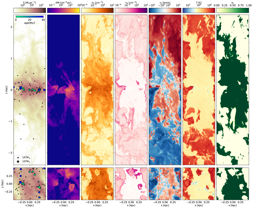
Figure 2: A sample post-processed snapshot at $t=551\,{\rm Myr}$ with total ionizing photon rate $Q_{\rm i}=8.0\times\times 10^{50}\,{\rm s}^{-1}$. The far left panels show the gas surface density projected along the $y$- (top) and $z$-directions (bottom). The projected positions of the star/sink particles are shown as colored circles, with size and color indicating mass and mass-weighted age ($t_{\rm sp}$), respectively. Runaway stars are shown as black dots. Continuing to the right, the panels show the EM (integrated electron density squared, ${\rm EM}=\int n_{\rm e}^{2}d\ell$), slices through the center of the simulations box of hydrogen number density $n_{\rm H}$, electron number density $n_{\rm e}$, vertical velocity $v_{z}$, gas temperature $T$, and neutral fraction $x_{\rm n}=n_{\rm H^{0}}/n_{\rm H}$. The full vertical extent of the simulation domain is $-3.584\,{\rm kpc}<z<3.584\,{\rm kpc}$.

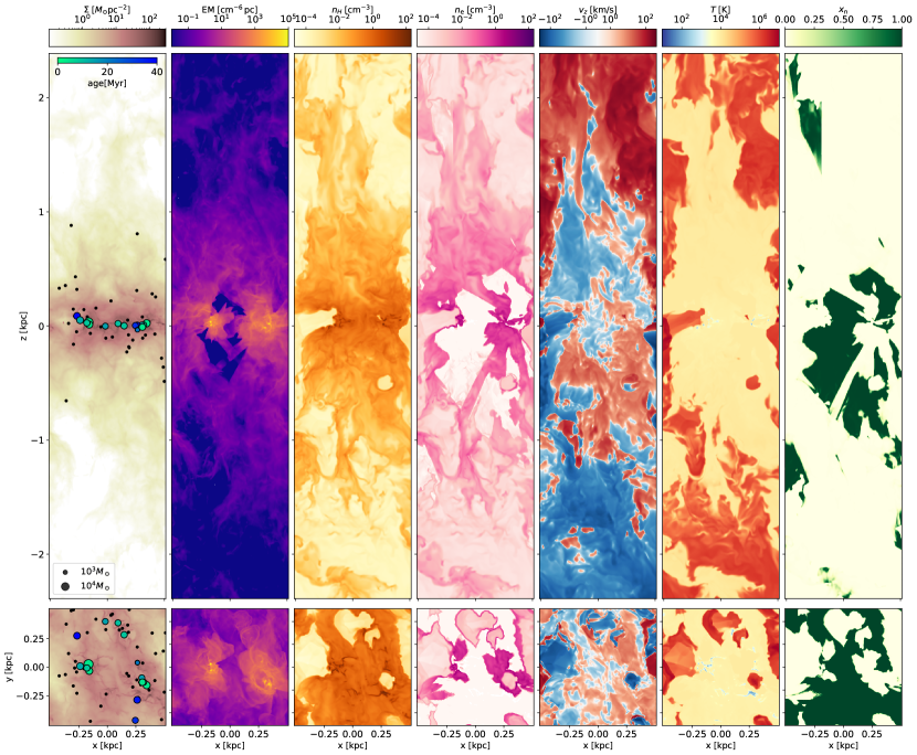
Figure 3: Same as Figure 2, but at $t=555\,{\rm Myr}$ when $Q_{\rm i}=1.1\times 10^{51}\,{\rm s}^{-1}$. With only $4\,{\rm Myr}$ time difference from the snapshot in Figure 2, the density, temperature, and velocity structure has changed little. However, the WIM layer is significantly more extended than in Figure 2, as can be seen in the projected electron density (EM, third panel from left) and electron density slice (fourth panel from right), and neutral fraction (rightmost panel).

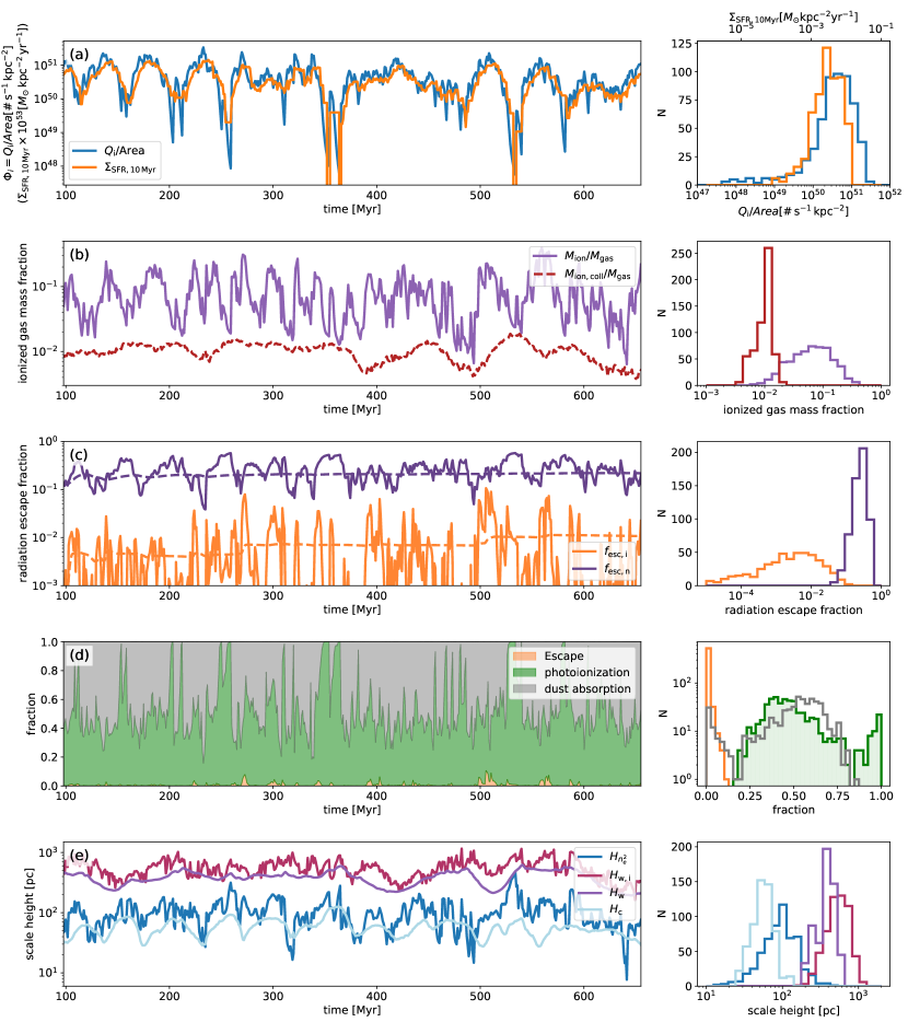
Figure 4: The time evolution (left) and distribution over time (right) of various box-integrated quantities. Row (a): Ionizing photon rate per unit area ($\Phi_{\rm i}=Q_{\rm i}/(L_{x}L_{y})$, in photon s^-1 kpc^-2) is shown in blue. The $10\,{\rm Myr}$ averaged star formation rate surface density is shown in orange. Row (b): The fraction of ionized (photoionization + collisional ionization) mass is shown by the solid curve (violet), while the fraction of collisionally ionized mass is shown by the dashed curve (crimson). Row (c): The escape fractions of ionizing (orange) and non-ionizing (purple) radiation. The solid and dashed lines plot instantaneous and cumulative escape fractions, respectively. Row (d): The fraction of ionizing photons that escape from the box (orange), photoionize neutral hydrogen (green), and are absorbed by dust (grey). Row (e): Scales heights, defined as rms distance from the midplane, of various components (Equation 5). Shown are warm ionized gas (magenta), total warm gas (purple), and cold gas (light blue), as well as $n_{\rm e}^{2}\propto{\rm EM}$ (dark blue).

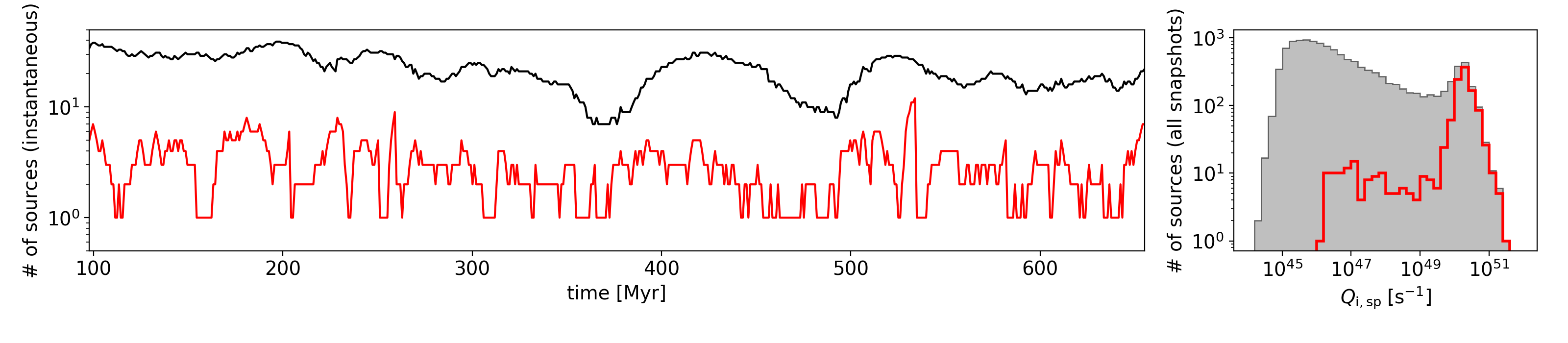
Figure 5: Left: total number of ionizing source particles (black) and the number luminous source particles needed to account for $>90\%$ of the total ionizing photon rate (red) as functions of time. Right: distribution of the ionizing photon rate of source particles $Q_{\rm i,sp}$ for all snapshots. As in the left panel, the grey histogram shows the distribution for all sources, while the red unfilled histogram shows the distribution for the brightest clusters that are responsible for $>90\%$ of $Q_{\rm i}$. Although we include all star particles with $t_{\rm sp}<40\,{\rm Myr}$ as active ionizing sources for a given snapshot, the total ionizing photon budget is dominated by a few young clusters.

3 Results

Here we present the results of the post-processing described above. We first examine the overall evolution of the simulation and tracked quantities therein, including statistics for radiation sources and sinks. We then analyze properties of warm ionized gas, including vertical profiles, volume filling factor, scale heights, and various statistical measures of the EM distribution. We also present synthetic ${\rm H}\alpha$ line profiles, commenting on comparisons to the WHAM (Wisconsin ${\rm H}\alpha$ Mapper, Reynolds et al., 1998) survey and prospects for identifying DIG based on spatially integrated velocity information. Comparison of our results to observations of gas scale heights in the Milky Way and external galaxies will be made in Section 4.

3.1 Overall Evolution

After $\sim 100\,{\rm Myr}$, the MHD simulation reaches a quasi-steady state in which the star formation rate (SFR) is self-regulated and ISM phases are in balance. The energy input from newly formed stars stirs turbulent motions and heats the ISM, maintaining the (turbulent + magnetic + thermal) pressure to offset the vertical weight of the ISM disk and hence to prevent runaway gravitational collapse. Meanwhile, expansion of hot superbubbles created by clustered SNe drives multiphase outflows consisting of hot winds and warm fountains. While the hot phase outflow achieves high enough velocity to escape into the galaxy’s halo, most of the warm phase outflow has $|v_{z}|<100\,{\rm km}\,{\rm s}^{-1}$ and is unable to overcome the large-scale gravitational potential, falling back onto the disk eventually. Averaged over several star-formation cycles, the properties of the hot wind and warm fountain are in a statistically steady state (see Kim & Ostriker 2017, 2018; Vijayan et al. 2019 for more quantitative analyses of star formation rate, thermal phase balance, and outflow properties).

To illustrate the structure of the ISM in the post-processed TIGRESS simulations, Figure 2 and Figure 3 show two example snapshots at $t=551\,{\rm Myr}$ and $555\,{\rm Myr}$. Each figure shows, from left to right, projections of the gas density ($\Sigma=\int\rho d\ell$, overlaid with star particle positions), emission measure (${\rm EM}=\int n_{\rm e}^{2}d\ell$), slices of hydrogen number density ($n_{\rm H}$), free electron number density ($n_{\rm e}$), gas velocity in the vertical direction ($v_{z}$), gas temperature ($T$), and neutral fraction ($x_{\rm n}$). The projections are along the $y$-axis (equivalent to the azimuthal direction; top panels) or $z$-axis (vertical direction; bottom panels), while slices are through $y=0$ (top) or $z=0$ (bottom).

To provide a sense of the physical scope and the dynamic range of our model, Figure 4 shows the time evolution (left) and distributions over time (right) of various global quantities. Table 2 provides a summary of statistical properties for these quantities: ionizing photon rate, star formation rate, mass fraction of ionized gas, escape fraction of ionizing and non-ionizing photons, fraction of photons lost to photoionization and dust absorption, and scale heights of the various gas components.

As shown qualitatively in Figure 2 and Figure 3, and quantitatively in Figure 4, both the structure and the extent of the WIM are highly variable in space and time. This variability is driven by the variability of $Q_{\rm i}$ and the presence or absence of escape channels for ionizing photons surrounding ionizing sources (see Section 3.1.1 and Section 3.2). For example, the distributions at $t=555\,{\rm Myr}$ in Figure 3 shows both inflowing and outflowing regions with a significant extraplanar DIG layer extending over $1\,{\rm kpc}$ from the midplane. By contrast, in the snapshot at $t=551\,{\rm Myr}$ (Figure 2) there is relatively little warm ionized gas far from the midplane (based on lower EM at large $|z|$), despite these snapshots being separated by just $\sim 4\,{\rm Myr}$, possessing a similar ionizing photon rate, and having a similar outflow rate of warm gas. This demonstrates the importance of radiative transfer to the DIG, which adds to the significant time variability already demonstrated for the ISM flow in the TIGRESS simulation. In spite of the time variability, we find that the existence of an extended WIM profile is commonplace.

We note that while the slices of $x_{\rm n}$ show that gas is either fully neutral or fully ionized because we evolve to equilibrium, at low density the recombination rate is low enough that in reality gas may remain partially-ionized even when not directly exposed to radiation (e.g., Dong & Draine, 2011). Evaluation of the importance of this effect for enhancing the DIG will require inclusion of ray-tracing and ionization/recombination in future time-dependent simulations.

3.1.1 Star formation, ionizing photon budget, and source properties

Row (a) in Figure 4 shows that the SFR per unit area $\Sigma_{\rm SFR,10\,{\rm Myr}}$ (orange, calculated from the mass of star particles with $t_{\rm sp}<10\,{\rm Myr}$) exhibits significant temporal fluctuations. The resulting ionizing photon production rate per unit area $\Phi_{\rm i}\equiv Q_{\rm i}/(L_{x}L_{y})$ (blue) is well correlated with $\Sigma_{\rm SFR,10\,{\rm Myr}}$, with a more pronounced fluctuation amplitude. The typical ionizing photon rate per unit area is $\Phi_{\rm i}=Q_{\rm i}/(L_{x}L_{y})=4.2_{-2.3}^{+4.0}\times 10^{7}$ s^-1 cm^-2 ($4.0_{-2.2}^{+3.8}\times 10^{50}$ s^-1 kpc^-2), which is roughly consistent with the observational estimate $5.2\times 10^{7}\,{\rm s}^{-1}\,\,{\rm cm}^{-2}$ in the solar neighborhood (McKee & Williams 1997; see also Abbott 1982; Dove & Shull 1994; Vacca et al. 1996). An overview of the summary statistics for the quantities shown in Figure 4 is given in Table 2.

One reason for the strong variability in the DIG is that a small number of sources are responsible for most of the ionization, and as a result localized absorption near the midplane can cast large volumes at high latitude into ionization “shadows.” The left panel of Figure 5 shows the time evolution of the number of active ionizing sources (black) and the minimum number of ionizing sources to account for 90% of the total ionizing photon rate (red). While there are 22 active ionizing sources on average, the majority of the ionizing photon budget is supplied by just a few ($\sim 3$) luminous sources with $t_{\rm sp}\lesssim 5\,{\rm Myr}$. The right panel of Figure 5 shows the distributions over time of the ionizing photon rate of all individual sources (grey) and of the sources that make up $>90\%$ of the total ionizing photon rate (red), which indicates that young star clusters with $Q_{\rm i,sp}\sim 10^{50}\,\,{\rm s}^{-1}$ dominate the ionizing photon production. The cutoff at $Q_{\rm i,sp}\sim 10^{45}\,{\rm s}^{-1}$ in the grey histogram is caused by the choice $40\,{\rm Myr}$ as the maximum age of ionizing sources.

3.1.2 Mass of Ionized Gas

Row (b) of Figure 4 (crimson line) shows that the mass of collisionally ionized gas that would be produced by supernova shocks in the absence of photoionization in the MHD simulation (i.e., $\int n_{\rm H}\gamma_{\rm coll}/(\gamma_{\rm coll}+\alpha_{\rm B})dV$) is only $\sim 1\%$ of the total gas mass. Including photoionization in the post-processing boosts the ionized mass fraction significantly (violet line), unless there is little recent star formation. The ionized gas mass fraction shown in Figure 4 includes both dense and diffuse components. We find that the low-density DIG at $|z|>200\,{\rm pc}$ is substantial in mass, but not in emission (see also Section 3.5), because the emissivity is proportional to $n_{\rm e}^{2}$. The mass of DIG at $|z|>200\,{\rm pc}$ represents $\sim 7\%$–$76\%$ of the total ionized gas mass with a mean of $40\%$. In contrast, the fraction of the total ${\rm H}\alpha$ emission originating from DIG at $|z|>200\,{\rm pc}$ is minor, ranging from $5.6\times 10^{-5}$ to $0.36$ with a mean of $0.05$.

3.1.3 Gas Scale Heights

Row (e) of Figure 4 shows the time evolution and distributions of the scale heights of warm ($H_{\rm w}$), warm ionized ($H_{\rm w,i}$), and cold ($H_{\rm c}$) gas. In addition, we show the scale height of emissivity from warm ionized gas $\propto n_{e}^{2}$ ($H_{n_{\rm e}^{2}}$). The two-phase (cold + warm) scale height (not shown) is approximately equal to the total warm gas scale height.

The reported scale heights are defined as

$$H_{q}\equiv\sqrt{\frac{\int\langle q\rangle z^{2}dz}{\int\langle q\rangle dz}}$$ (5)

where the brackets $\langle\cdot\rangle$ denotes the horizontal average, and the $q$ is the quantity over which the scale height is computed (e.g. the number density ($n_{\rm H}$), free electron density ($n_{\rm e}$), or the square of the electron density ($n_{\rm e}^{2}$) of a cold or warm phase).

The median scale height of (star-forming) cold gas is only $55\,{\rm pc}$, which is roughly comparable to the $Q_{\rm i}$-weighted scale height of the ionizing sources ($38\,{\rm pc}$). Both are in turn roughly comparable to the Gaussian scale height of O-B5 stars of $63\,{\rm pc}$ measured by Hipparcos (Maíz-Apellániz, 2001). The warm gas scale height fluctuates between about $250\,{\rm pc}$ and $500\,{\rm pc}$, with a median value of $393\,{\rm pc}$. The scale height of warm ionized gas is somewhat larger, with a median value of $540\,{\rm pc}$. The median value of $H_{n_{\rm e}^{2}}$ is only $94\,{\rm pc}$, considerably smaller than $H_{\rm w,i}$, and only slightly larger than $H_{c}$. This suggests that the dense ionized gas near ionizing sources constitutes a major fraction of the total emission from warm ionized gas (see Section 3.5). For this reason, the scale heights of WIM ($H_{\rm w,i}$ and $H_{n_{\rm e}^{2}}$) derived from Equation 5 can be quite different from observational scale heights derived from different approaches (e.g., by fitting an exponential to the vertical component of EM or DM, excluding dense ionized gas). We defer detailed the analysis of WIM scale height and its comparison to observations until Section 3.4.

Table 2: Summary Statistics of Selected Properties

	$\Sigma_{\rm SFR,10Myr}$	$\Phi_{\rm i}$	$M_{\rm ion}/M_{\rm gas}$	$f_{\rm esc,i}$	$f_{\rm dust,i}$	$f_{\rm esc,n}$	$H_{\rm c}$	$H_{\rm w}$	$H_{\rm w,i}$	$H_{n_{\rm e}^{2}}$
	$\left(\dfrac{10^{-3}M_{\odot}}{\,{\rm kpc}^{2}\,{\rm yr}}\right)$	($10^{50}{\rm s}^{-1}\,{\rm kpc}^{-2}$)	(%)	(%)	(%)	(%)	(pc)	(pc)	(pc)	(pc)
(1)	(2)	(3)	(4)	(5)	(6)	(7)	(8)	(9)	(10)	(11)
25th	1.51	1.82	3.38	0.02	40.0	17.2	44.4	301	423	65.0
50th	2.98	3.99	6.30	0.19	53.0	24.8	55.4	393	541	94.2
75th	5.84	7.79	10.2	0.82	61.4	33.9	68.0	460	680	134
Mean	4.00	5.54	8.29	1.08	57.1	21.8	57.5	384	557	105

Note. — Column (1) Summary statistic (percentile or mean) Column (2) Star formation rate per unit area averaged over $10\,{\rm Myr}$. Column (3) mass fraction of ionized gas. Column (4) Ionizing photon rate per unit area. Column (5) Escape fraction of ionizing radiation. Column (6) Dust absorption fraction of ionizing radiation. Column (7) Escape fraction of non-ionizing radiation. Columns (8)–(11) Scale height of cold, warm, warm ionized, and $n_{\rm e}^{2}$ (see Equation 5).

3.2 Escape fraction and dust absorption fraction

The escape of ionizing radiation from star-forming galactic disks is key to understanding the cosmic reionization and intergalactic UV background. However, constraints on the galaxy-scale escape fraction remain highly uncertain (Dayal & Ferrara, 2018). Here, we compare the fraction of ionizing photons that escape the domain to the fraction that are being absorbed by gas (neutral hydrogen) and dust. The instantaneous escape fraction of ionizing radiation is estimated as $f_{\rm esc,i}=(Q_{\rm exit,i}+Q_{\rm lost,i})/Q_{\rm i}$, where $Q_{\rm exit,i}$ is the rate of ionizing photons that exit through the vertical boundary of the computational domain, and $Q_{\rm lost,i}$ is the ionizing photon rate of “lost” photon packets that are terminated by the condition $d_{\rm xy}>d_{\rm xy,\rm max}=1024\,{\rm pc}$. The gas and dust absorption fractions are calculated as $f_{\rm gas,i}=\int\mathcal{I}_{\rm phot}dV/Q_{\rm i}$ and $f_{\rm dust,i}=\int\mathcal{D}_{\rm i}dV/Q_{\rm i}$, respectively, where $\mathcal{D}_{\rm i}=n_{\rm H}\sigma_{\rm d,i}c\mathcal{E}_{\rm i}/(h\nu_{\rm i})$ is the local dust absorption rate.

The solid orange line in row (c) of Figure 4 shows that the instantaneous escape fraction varies with time significantly, with the cumulative escape fraction ($\int Q_{\rm esc,i}dt/\int Q_{\rm i}dt$) of $1.1\%$ (orange dashed line). The large temporal fluctuation in $f_{\rm esc,i}$ arises because (1) ionizing sources have short lifetimes, and the total $Q_{i}$ is dominated by a small number of sources, (2) ionizing photon sources are near the midplane, where dense gas absorbs most of the photons and blocks large volumes of distant gas, and (3) complete escape of ionizing photons from the galaxy requires very low-density pathways extending over several kpc, created by strong hot winds powered by multiple recent supernovae (Dove et al., 2000). Since the low density channels must align favorably with young, unshielded ionizing sources, conditions allowing ionized photon escape occur only rarely and intermittently. While there is no significant correlation between $\Phi_{\rm i}$ and $f_{\rm esc,i}$, we find that relatively high escape fraction ($\gtrsim 3\%$) occurs only if $\Phi_{\rm i}>5\times 10^{49}\,{\rm kpc^{-2}}\,{\rm s}^{-1}$. This trend is expected given that higher $\Phi_{\rm i}$ allows ionizing photons to penetrate larger distances, increasing the chances of escape (e.g., Dove & Shull, 1994; Dove et al., 2000; Haffner et al., 2009). Our time-averaged escape fraction is in agreement with the observational estimate of $\sim 1$–$2\%$ based on ${\rm H}\alpha$ emission from high velocity clouds (e.g., Bland-Hawthorn & Maloney, 2002).

The escape fraction of non-ionizing radiation $f_{\rm esc,n}$ is limited only by dust absorption and is significantly higher than $f_{\rm esc,i}$, with a time-averaged (cumulative) escape fraction of $\sim 22\%$ (see Column (7) of Table 2). The large discrepancy for galaxy-scale escape fraction between ionizing and non-ionizing radiation is in contrast to the results found from radiation hydrodynamic simulations of star-forming molecular clouds. In particular, Kim et al. (2019) found that $f_{\rm esc,n}$ and $f_{\rm esc,i}$ are quite similar over most of the evolution, for a range of cloud masses and sizes. In conditions of a star-forming cloud, the ionization parameter is much higher, which results in similar values of $f_{\rm esc,n}$ and $f_{\rm esc,i}$ (see below).

Row (d) of Figure 4 shows that dust grains contribute significantly to the absorption of ionizing photons, reaching up to $\sim 50\%$ of events globally. We find that the majority of absorption events by both neutral hydrogen and dust occur in high density gas within $200\,{\rm pc}$ from the midplane. Globally, 50% of the absorption by neutral hydrogen occurs at density above $n_{\rm H}=15\,{\rm cm}^{-3}$, while 50% of the absorption by dust occurs at density above $n_{\rm H}=56\,{\rm cm}^{-3}$.

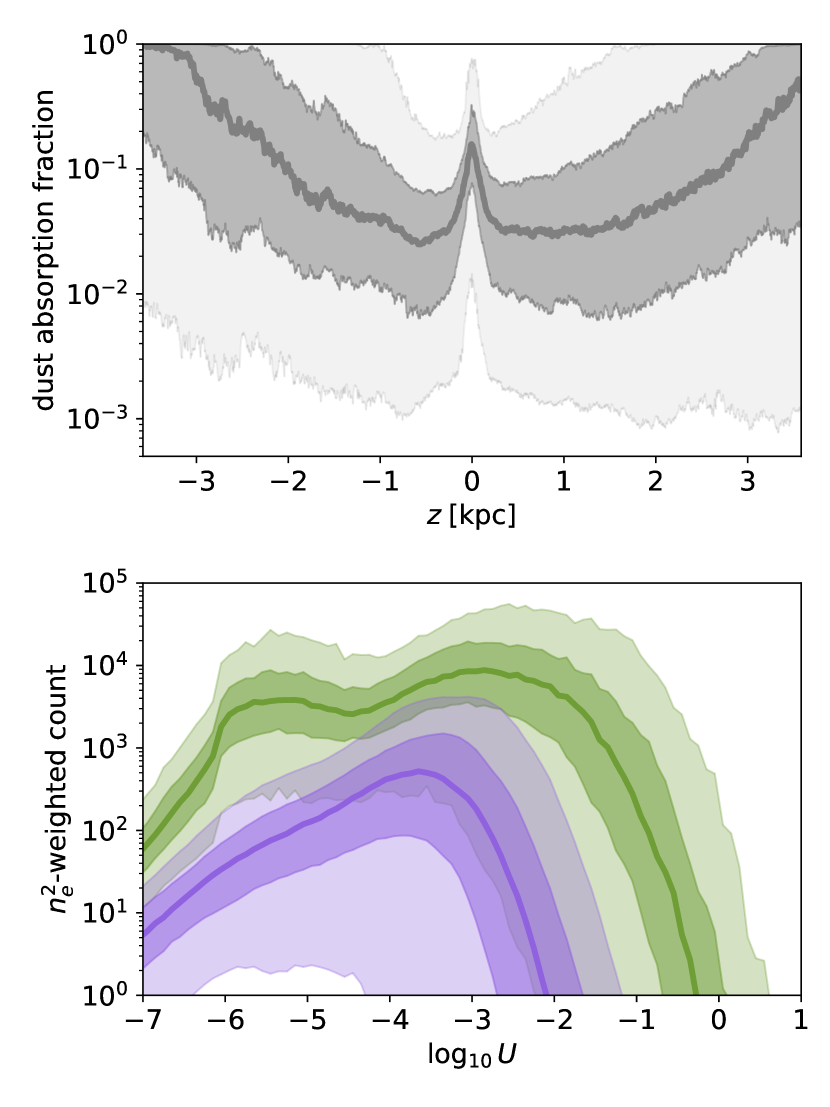
Figure 6: Top: Time-averaged, horizontally averaged fraction of ionizing photons that are absorbed by dust grains, $q_{\rm i,dust}$, as defined in Equation 6, as a function of height from the midplane. The heavy curve shows the median profile, while the shaded regions bound the 25^th to $75^{\rm th}$ percentiles (dark shaded region) and $5^{\rm th}$ to 95^th percentiles (light shaded region). Bottom: Time-averaged distribution of the local ionization parameter $U=\mathcal{E}_{\rm i}/(h\nu_{\rm i}n_{\rm H})$, weighted by the local photoionization rate for gas within (green) and above (purple) 200 pc from the midplane. For both, the shaded regions bound the regions between the 25^th to 75^th and 5^th to 95^th percentiles. The majority of photoionization (and recombination) takes place in dense gas near the midplane, which has a systematically higher ionization parameter than gas at high altitudes. This creates the overall shape seen in the top panel, where the relative importance of dust is highest near the midplane.

Figure 6 characterizes the relative importance of dust absorption vs. photoionization. In the top panel, we show the time-averaged (median) vertical profile of the area-averaged dust absorption fraction, defined as

$$q_{\rm dust,i}=\frac{\langle\mathcal{D}_{\rm i}\rangle}{\langle\mathcal{I}_{\rm phot}\rangle+\langle\mathcal{D}_{\rm i}\rangle}\,.$$ (6)

Most of the time the dust absorption rate is a factor of $5$–$10$ lower than the photoionization rate near the midplane, and a factor of $\sim 50$ lower at $|z|\gtrsim 1\,{\rm kpc}$. This low median value of $\langle q_{\rm dust,i}\rangle$ might seem hard to reconcile with the time-averaged (cumulative) global dust absorption fraction of 57% (Column (6) of Table 2). However, we note that the majority of dust absorption events take place in dense gas (of size a few tens of pc) near bright sources, whose vertical position changes from snapshot to snapshot. As a result, the distribution of $q_{\rm dust,i}$ at each height is strongly skewed toward high values; the median value represents the typical absorption fraction in “diffuse” part of the ISM.

Assuming that WIM gas is near-fully ionized ($n_{\rm e}\approx n_{\rm H}$) and in photoionization–recombination equilibrium ($\mathcal{I}_{\rm phot}\approx\mathcal{R}$), one can show that the local dust absorption rate is greater than the photoionization rate if

$$U\gtrsim\alpha_{\rm B}/(c\sigma_{\rm d,i})\sim 10^{-2}$$ (7)

where $U\equiv\mathcal{E}_{\rm i}/(h\nu_{\rm i}n_{\rm H})$ is the the local ionization parameter (e.g., Dopita et al., 2003; Kim et al., 2019). The bottom panel of Figure 6 shows the time-averaged distribution of $U$ weighted by the local recombination rate, for warm gas within (green) and above (purple) 200 pc from the midplane. Most of ${\rm H}\alpha$ emitting ionized gas is at low altitudes (as shown by the distribution of $H_{n_{\rm e}^{2}{}}$ in Figure 4, row (e)), where the ionization parameter is $U\sim 10^{-4}$–$10^{-1.5}$. In contrast, the WIM at high altitudes has a systematically lower ionization parameter $U\sim 10^{-5}$–$10^{-3}$. These differences in ionization parameter explain the relative roles of dust and gas in absorbing ionizing photons at the midplane (where $U$ is larger and dust absorption can exceed gas absorption) vs. high altitudes (where $U$ is smaller and absorption by gas always dominates).

3.3 Vertical Profiles and Volume Filling Factors

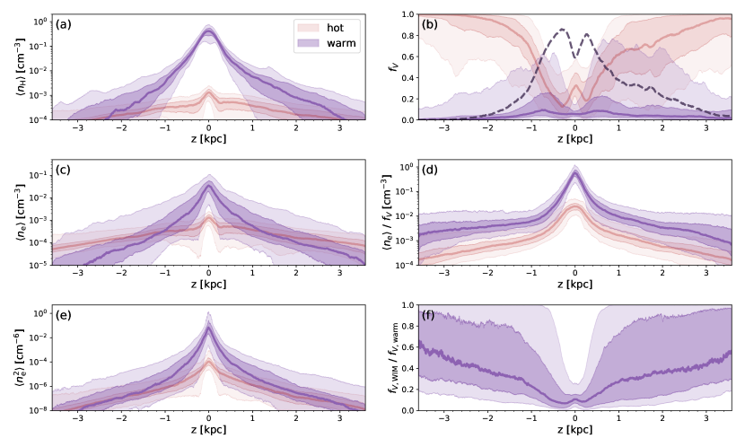
Figure 7: Time-averaged, horizontally-averaged $z$ profiles of $n_{\rm H}$ (panel (a)), the volume filling factors $f_{V}$ (panel (b)), $n_{\rm e}$ (panel (c)), the characteristic electron density ($\langle n_{\rm e}{}\rangle/f_{V}$, panel (d)), $n_{\rm e}^{2}$ (panel (e)), and the volume fraction of ionized gas within the warm medium ($f_{V,\rm WIM}/f_{V,\rm warm}$, panel (f)). In each panel, the purple curve shows the median profile of the (selected) warm gas ($5050\,{\rm K}<T<2\times 10^{4}\,{\rm K}$), while the red curve shows the median profile of the hot gas ($T>2\times 10^{4}\,{\rm K}$). Dark and light shaded regions indicate the 25^th–75^th and 5^th–95^th percentiles. In (b), the solid curve shows the volume filling factor for the WIM, while the dashed curve shows the volume filling factor for all warm gas, regardless of the ionization state.

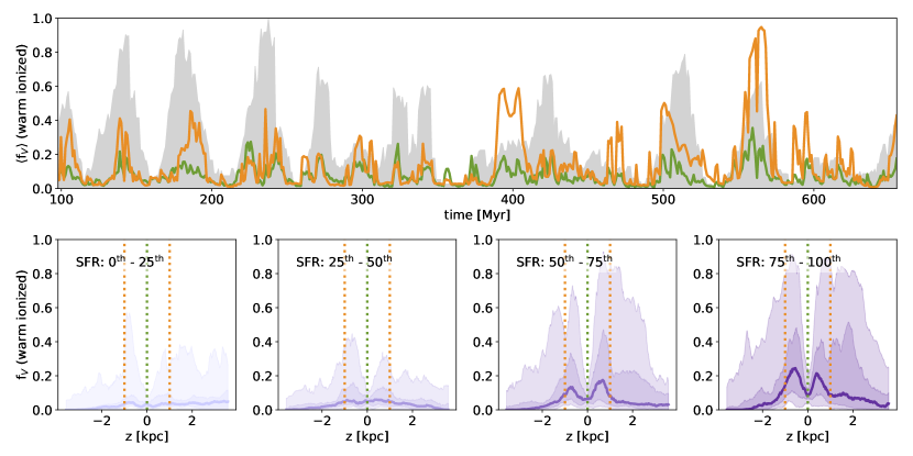
Figure 8: Top: Horizontally averaged volume filling fraction of warm ionized gas ($f_{V,{\rm WIM}}$) as a function of time for gas at $|z|<200\,{\rm pc}$ (green) and for gas at $800\,{\rm pc}<|z|<1200\,{\rm pc}$ (orange). The grey shade is the rescaled SFR for comparison. Bottom: the average z-profile of $f_{V,{\rm WIM}}$ in bins of $\Sigma_{{\rm SFR},{\rm 10Myr}}$. The solid curve shows the median z-profile, while the shaded regions show the 25^th-75^th and 5^th-95^th percentiles. The dotted lines show the central positions of the slices shown in the top panel.

As described in Kim & Ostriker (2018); Vijayan et al. (2019), spatio-temporally correlated SNe in our simulation launch multiphase outflows consisting of hot winds and warm fountains. Although hot winds attain high enough velocity ($>200\,{\rm km}\,{\rm s}^{-1}$ at $|z|>1\,{\rm kpc}$) to develop into galaxy-scale winds, the velocity distribution of warm outflows is exponential with the typical outflow velocity of $\sim 60\,{\rm km}\,{\rm s}^{-1}$ at $|z|=1\,{\rm kpc}$. This is insufficient to escape from the gravitational potential well of the Milky Way, and as a result, most of warm outflows eventually fall back toward the midplane as inflows. The vertically stratified density profile results from the weight of gas balancing the Reynolds stress associated with the outflow momentum flux (plus thermal and magnetic pressure support).

Figure 7 shows as solid lines the time-averaged (median) vertical profiles of $\langle n_{\rm H}\rangle$, $\langle n_{\rm e}\rangle$, $\langle n_{e}^{2}\rangle$, the volume filling-factor $f_{V}$, $\langle n_{\rm e}\rangle/f_{V}$, and $f_{\rm V,WIM}/f_{\rm V,w}$, where $\langle\rangle$ refers to the area-average over the $x$-$y$ plane. The warm gas profiles are shown in purple, while hot gas profiles are shown in red. Note that $\langle n_{\rm e}\rangle/f_{V}$ is the density of ionized gas averaged over the volume occupied by itself, i.e., it is the characteristic local density of ionized gas.

The time-averaged (median) midplane densities of warm and warm ionized gas (panels (a) and (c) in Figure 7) are at $0.41\,{\rm cm}^{-3}$ and $0.032\,{\rm cm}^{-3}$, respectively, as measured within $50\,{\rm pc}$ of the midplane. In panel (b), the volume filling factors of total warm gas (dashed line) and WIM (purple) show depressions near the midplane as this is where most hot gas is generated via shock heating by supernovae. The total warm gas volume filling factor peaks at $f_{V,{\rm warm}}\sim 0.86$ near $|z|\sim 300\,{\rm pc}$. At $z\gtrsim 2\,{\rm kpc}$, the volume filling factors of both warm and warm ionized gas (Figure 7(b)) become increasingly small as the box becomes dominated by the hot winds. However, the share of warm gas that is ionized (i.e. $f_{V,{\rm WIM}}/f_{V,{\rm w}}$) increases as a function of distance from the midplane (Figure 7(f)). The characteristic number density $\langle n_{\rm e}\rangle/f_{V}$ for WIM ranges between $9\times 10^{-3}\,{\rm cm}^{-3}{}$ (25^th percentile) and $5\times 10^{-2}\,{\rm cm}^{-3}$ (75^th percentile) for $0.2\,{\rm kpc}<|z|<1\,{\rm kpc}$ (Figure 7(d)). The vertical profile of $\langle n_{\rm e}^{2}\rangle$ (Figure 7(e)) for warm gas is sharply peaked around the midplane, suggesting that most of ${\rm H}\alpha$ emission from warm ionized gas would originate near the disk midplane.

The volume filling factor of warm ionized gas is also correlated, albeit with large temporal variance, with the global SFR in the box. The top panel in Figure 8 shows the time evolution of the average volume filling factor of warm ionized gas within $200\,{\rm pc}$ from the midplane (green) and within $200\,{\rm pc}$ from $z=1\,{\rm kpc}$ (orange). For reference, the grey shaded area shows $\Sigma_{\rm SFR,10\,{\rm Myr}}$ (scaled such that $\max(\Sigma_{\rm SFR,10\,{\rm Myr}})=1$). In general, the warm ionized gas volume filling factor is relatively small near the midplane, with a median [25^th, 75^th] value of 0.057 [0.031, 0.097] at $|z|<200$pc.

In contrast to the midplane region, the volume filling factor of the WIM at $0.8\,{\rm kpc}<|z|<1.2\,{\rm kpc}$ exhibits relatively large temporal fluctuations. In particular, the warm ionized gas near $1\,{\rm kpc}$ off the midplane accounts for the majority of the volume ($f_{V,{\rm WIM}}>0.5$) for 8.4% of the timesteps, and accounts for at least 25% of the volume ($f_{V,{\rm WIM}}>0.25$) for 18% of the timesteps. However, we note that the majority of our snapshots are not dominated by WIM at $z=1\,{\rm kpc}$; the median (mean) $f_{V,{\rm WIM}}$ at this height is 0.062 (0.15).

In the bottom panels of Figure 8 we show the average distribution of $f_{V,{\rm WIM}}$ as a function of height off the midplane, binned by quartile of the SFR ($10\,{\rm Myr}$ average). Although there is not a strict correspondence between the SFR and the volume filling factor of the warm ionized gas near $1\,{\rm kpc}$, the volume filling factor tends to rise with increasing SFR, in particular the high-$f_{V}$ tail of the distribution.

3.4 Scale heights of ionized gas emission

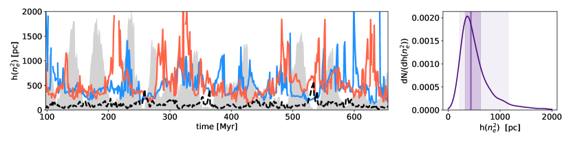
Figure 9: Left: The time evolution of the exponential-fit scale height $h(n_{\rm e}^{2})$. The exponential-fit scale height includes only gas at $|z|>1$ kpc. The red and blue curves show the scale height above and below the midplane, respectively. The black dashed curve shows the $n_{\rm e}^{2}{}$ rms scale height ($H_{n_{\rm e}^{2}{}}$), defined as in Equation 5. The grey shade shows the (scaled) SFR for comparison. Right: The distribution of the exponential-fit scale height over all time, both above and below the midplane. The thick purple line shows the median value of the scale height, while the shaded regions show the 25^th to 75^th percentile range.

In this study, the scale height of warm ionized gas is measured in two different ways: (1) the rms distance from the midplane ($H_{\rm w,i}$ and $H_{n_{\rm e}^{2}}$, as described in Section 3.1.3); and (2) a fit of the vertical profile of $n_{\rm e}^{2}$ to an exponential function above some height from the midplane. In this section, we describe our procedure and results for the latter, which is more relevant to existing measurements of the DIG in external galaxies.

Most extragalactic observational studies measuring scale heights of the DIG from ${\rm H}\alpha$ emission exclude the region closest to the midplane due to concerns regarding contamination from H II regions, dust extinction, and beam smearing (e.g., Levy et al., 2019; Boettcher et al., 2019). To make a more fair comparison to extragalactic measures of the ${\rm H}\alpha$ scale height, we fit an exponential profile to the vertical profile of $\langle n_{\rm e}^{2}\rangle$, considering only the high-altitude region with $|z|>1\,{\rm kpc}$. The left panel of Figure 9 shows the time evolution of this exponential-fit $n_{\rm e}^{2}$ scale height, $h(n_{\rm e}^{2})$, measured for regions above (red) and below (blue) the midplane. In the right panel, we show the probability density function of $h(n_{\rm e}^{2})$ marginalized over time and direction, obtained from kernel density estimation with a bandwidth of 0.25 (following Scott’s Rule, Scott 2015). The $n_{\rm e}^{2}{}$ exponential-fit scale height exhibits large temporal fluctuations in the range $\sim 0.2$–$2.0\,{\rm kpc}$, with no apparent correlation with recent star formation activity (grey shades). The distribution of $h(n_{\rm e}^{2})$ is right-skewed with a median value $437\,{\rm pc}$.

Because we have aggressively masked regions of box close to the midplane when computing this observational scale height, the overall trend effected by the exponential fit method is to increase the measured scale height (note that the median rms scale height of $n_{\rm e}^{2}$ is only $94\,{\rm pc}$). Interestingly, the tail of high exponential-fit scale heights ($h(n_{\rm e}^{2})>1\,{\rm kpc}$) is not correlated with large $H_{n_{\rm e}^{2}}$ (as defined by Equation 5). We note, as a caution, that there are significant differences in the ${\rm H}\alpha$ scale height as measured by an external observer ($h(n_{\rm e}^{2})$) and the scale height of WIM as defined by Equation 5 for the same snapshot. As shown in Figure 9, because the exponential-fit scale heights do not include the inner, steeper regions of the $n_{\rm e}^{2}{}$ profile (Figure 7c), they are systematically larger than the time-equivalent rms scale heights.

3.5 Distribution of $n_{\rm e}$

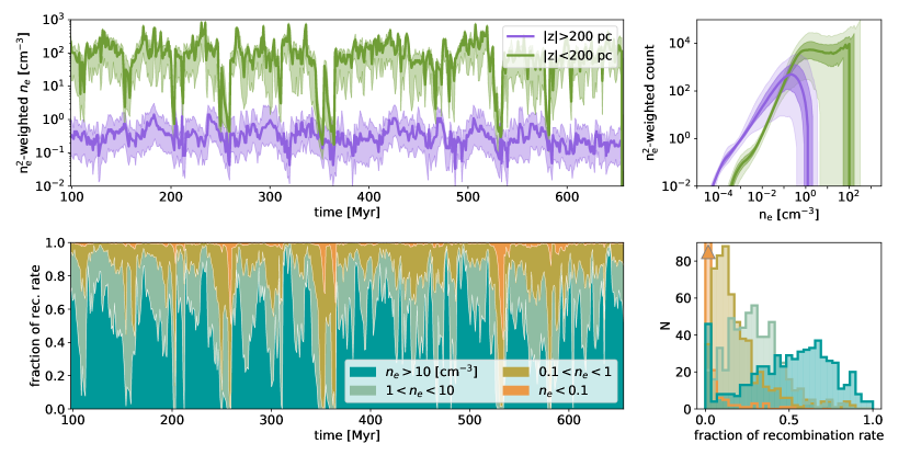
Figure 10: Top left: time evolution of the electron density weighted by $n_{\rm e}^{2}$ for gas at $|z|<200\,{\rm pc}{}$ (green) and $|z|>200\,{\rm pc}{}$ (purple). The dark curve shows the median value of the $n_{\rm e}$ distribution, while the shaded regions show the 25^th and 75^th percentiles. Top right: the time-averaged median distribution of recombination rate-weighted $n_{\rm e}$ distribution. The shaded regions show the 25^th to 75^th percentile and 5^th to 95^th percentile regions. Bottom left: time evolution of the fraction of the ${\rm H}\alpha$ recombination rate contributed by gas of a given electron density slice (see legend). Bottom right: the distribution over time of the recombination rate fractions shown at left. Again, the colors indicate slices in $n_{\rm e}$. The lowest density bin contributes $<3.4\%$ of the total recombination rate for $>90\%$ of the timesteps (N=523). For visual clarity, the figure is truncated at N=90; the orange triangle indicates that the lowest density bin extends to N=523.

To explore what fraction of ${\rm H}\alpha$ emission originates from low- versus high-density gas, we calculate the density distribution of warm ionized gas weighted by $n_{\rm e}^{2}$, which we take as a proxy for the local ${\rm H}\alpha$ emission rate. In Figure 10, the top-left panel shows the time evolution of the median and 25^th and 75^th percentiles in the distributions at height $|z|<200\,{\rm pc}$ (green) and at $|z|>200\,{\rm pc}$ (purple); the bottom-left panel shows the fraction of total recombination that originates from gas at different density slices. Right panels show the distributions over all time of $n_{e}$ (top) and the contribution to the recombination rate (bottom).

As expected, the total emission is dominated by low-altitude gas. Although the contribution of relatively dense gas ($n_{\rm e}>10\,{\rm cm}^{-3}$) dominates the total recombination rate budget, the moderate-density ionized gas with $1\,{\rm cm}^{-3}<n_{\rm e}<10\,{\rm cm}^{-3}$ also contributes significantly to the total. At $|z|<200\,\,{\rm pc}$, each logarithmic density interval above $n_{\rm e}\gtrsim 1\,{\rm cm}^{-3}$ contributes approximately equally to the ${\rm H}\alpha$ emission. At $|z|>200\,{\rm pc}$, most of ${\rm H}\alpha$ emission comes from gas with $0.1\,{\rm cm}^{-3}<n_{\rm e}<1\,{\rm cm}^{-3}$, but it accounts for, on average, only $\sim\!14\%$ of the total emission. The typical density of ${\rm H}\alpha$ emitting gas at high $|z|$ is roughly consistent with the observational estimate of the WIM density in the Solar neighborhood (e.g., Berkhuijsen & Müller, 2008).

3.6 Distribution of EM

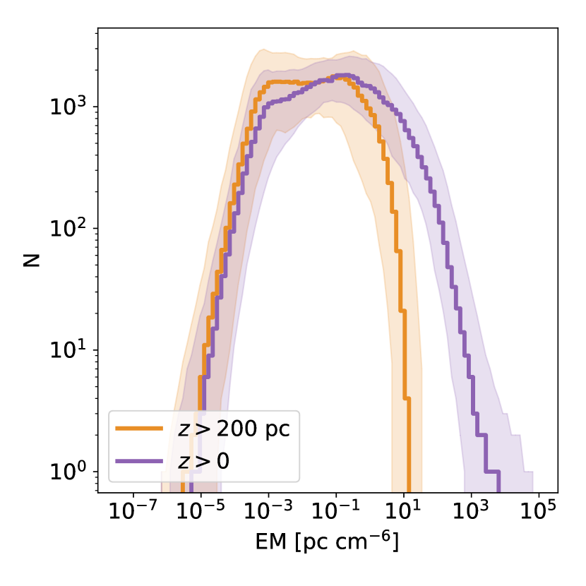
Figure 11: The distribution over time of EM ($=\int n_{\rm e}^{2}{}dz$) integrated over the plane of the disk, for an observer looking perpendicular to the plane of the disk and away from the midplane. The median distribution for an observer embedded in the midplane ($z>0$, purple) and an observer $200\,{\rm pc}$ away from the midplane ($z>200$ pc, orange) are shown by the thick stepped curves. The shaded regions show the 25^th and 75^th percentiles for both cases. The high-EM tail of the midplane observer (purple) is indicative of dense, high EM regions near the midplane; these are analogous to classical H II regions.

In Figure 11, we show the time-averaged (median) EM distribution integrated outward along the $z$-axis from $z=0$ (purple) and $z=200\,{\rm pc}$ (orange). In both cases, we take the (square) beam size to be the same as the grid resolution $\Delta x=4\,{\rm pc}$. The two distributions are similar at low EM ($\lesssim 1\,{\rm pc}\,{\rm cm}^{-6}$). At high EM, however, the two distributions sharply diverge, with the observer at the midplane seeing significantly more high EM instances than its counterpart at $200\,{\rm pc}$. This is a result of the contribution of dense gas near the midplane (see also Figure 10). The high-EM extension is equivalent to the contribution from classical H II regions, though we do not presently resolve such regions or model them self-consistently with dynamics. Because of the sensitivity of the EM distribution to the presence of dense material near the midplane, we note that it is crucial to fully exclude gas near the midplane in order to properly sample extraplanar warm ionized gas.

We now consider whether the width of the distribution of our EM measurements can be used to gauge the agreement with our results and measurements taken of the EM distribution of the WIM in the Milky Way. Hill et al. (2008) found that the distributions of the vertical component of EM from the WHAM survey is well characterized by a lognormal distribution with mean $\langle\log_{10}{\rm EM}_{\perp}({\rm pc}\,{\rm cm}^{-6})^{-1}\rangle=0.146$ and width $\sigma_{\log_{10}{\rm EM}_{\perp}}=0.19$. When considered with an effective beam size of $4\,{\rm pc}$, the width of our EM distribution does not match that of EM distributions for the solar neighborhood (Hill et al., 2008). However, this apparent width is degenerate with the physical size of the beam in question. As shown in Figure 12, increasing the number of cells that are considered in the measurement of the EM for a given line of sight decreases the width of the resulting EM distribution, as the beam averages over a larger area (see also Berkhuijsen & Fletcher, 2015). Because the beam size of the WHAM observation is an on-sky beam size rather than physical beam size, we cannot use the width of the EM distribution to test consistency of our models with the Milky Way.

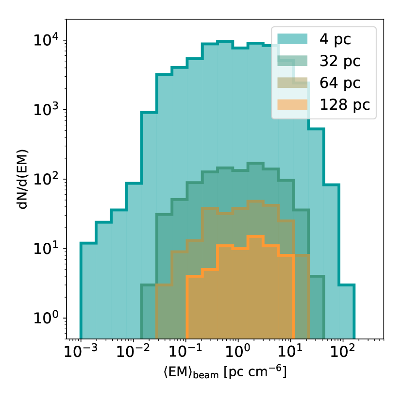
Figure 12: For a representative snapshot ($t=192\,{\rm Myr}$), the effect of increasing the effective physical beam size from between the fiducial resolution ($4\,{\rm pc}$) to $128\,{\rm pc}$. As the beam size increases, the width of the EM distribution shrinks while the mean value remains unchanged. This effect complicates comparison to the observed width of the (WHAM) EM distribution, as there is no single physical scale that corresponds to the angular beam size in observation.

3.7 The ${\rm H}\alpha$ line profile

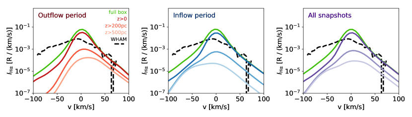
Figure 13: Time-averaged, horizontally averaged mean synthetic ${\rm H}\alpha$ line profiles for snapshots with bulk outflows at $z=1$ kpc (left, red), snapshots with bulk inflows at $z=1$ kpc (middle, blue), and all snapshots (right, purple). In each panel, the average WHAM line profile at $85\arcdeg<b<90\arcdeg$ is shown by the dashed black curve. All profiles are given as specific photon intensities in Rayleigh per $\,{\rm km}\,{\rm s}^{-1}$ (${\rm R}=10^{6}/(4\pi)\,{\rm photons}\,{\rm cm}^{-2}\,{\rm s}^{-1}{\rm sr}^{-1}$). The green curve shows the line profile as integrated across the full TIGRESS box; note that the presence of an outflow or inflow is determined by the top half of the box ($z>0$), and therefore does not necessarily correspond to an outflow or inflow in the bottom half of the box. The colored curves show, in order of increasing lightness, ${\rm H}\alpha$ line profiles as integrated from $z=0$, $z=200$ pc, and $z=500\,{\rm pc}{}$ to the top of the box.

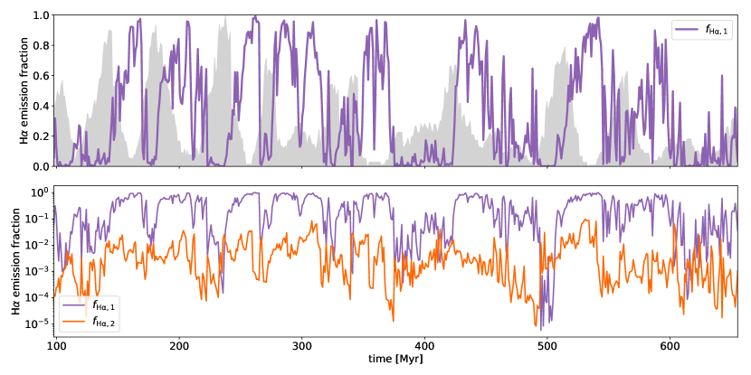
Figure 14: Top: The fraction of the high velocity ($v_{z}>50\,{\rm km}\,{\rm s}^{-1}$) ${\rm H}\alpha$ wing that is emitted from gas at $z>200\,{\rm pc}$ is shown in purple (Equation 9). For reference, the 10 Myr-averaged SFR is shown in grey. The apparent anticorrelation between the two suggests that the importance of high altitude ${\rm H}\alpha$ emission peaks approximately 20 Myr after the peak of star formation. Bottom: the fraction of high velocity ${\rm H}\alpha$ emission that originates from high altitudes is again shown in purple, as at top. The fraction of the total ${\rm H}\alpha$ emission that originates from high velocity gas is shown in orange (Equation 9).

Observations of high velocity gas have often been used to detect and quantitatively characterize the properties of galactic outflows (see, e.g. Hill et al., 2008; Wood et al., 2015; Cicone et al., 2016; Rodríguez del Pino et al., 2019). The integrated ${\rm H}\alpha$ line profiles constructed from TIGRESS thus both act as a benchmark for the simulation as compared to ${\rm H}\alpha$ surveys of the Solar neighborhood, and provide insight into the physical origin of high velocity gas seen in integrated line profiles of external galaxies.

To construct line-of-sight integrated profiles, we first compute the ${\rm H}\alpha$ photon emissivity of each cell as $j_{{\rm H}\alpha}(v)=(4\pi)^{-1}\alpha_{\rm eff,{\rm H}\alpha}n_{\rm e}^{2}\phi(v)$, where $\alpha_{\rm eff,H\alpha}=1.17\times 10^{-13}T_{4}^{-0.942-0.030\ln{T_{4}}}\,{\rm cm}^{3}\,{\rm s}^{-1}$ and the normalized line profile $\phi(v)$ is a Gaussian with thermal width $\sim\!\!9.1\,{\rm km}\,{\rm s}^{-1}{}$ (for a pure hydrogen gas at $T=10^{4}\,{\rm K}$) centered at the vertical velocity $v_{z}$ (Draine, 2011b). The line profile is obtained by integrating $j_{{\rm H}\alpha}(v)$ along the line of sight perpendicular to the midplane

$$I_{\rm H\alpha}(v)=\int_{z_{\rm min}}^{z_{\rm max}}j_{\rm H\alpha}(v)dz\,.$$ (8)

The effects of absorption and scattering by dust are ignored.

First, we consider mock “observations” made of the Milky Way DIG by constructing ${\rm H}\alpha$ line profiles integrated from a given $z_{\rm min}$ to the top of the box ($z_{\rm max}=+L_{z}/2$). For this exercise, we construct the line profiles using the top half of the box only (i.e. an observer looking perpendicular to the plane of the disk away from the midplane), and consider $z_{\rm min}=0,200\,{\rm pc}$, and $500\,{\rm pc}$ to separate contributions from dense and diffuse ionized gas. We also include the profile as integrated across the full box ($z_{\rm min}=-L_{z}/2$). In Figure 13, we show the time-averaged and horizontally-averaged mean line profiles for outflow states, inflow states and for all snapshots. The line intensity is given in units of Rayleigh per ${\rm km}\,{\rm s}^{-1}$ (${\rm R}=10^{6}/(4\pi)\,{\rm photons}\,{\rm cm}^{-2}\,{\rm s}^{-1}{\rm sr}^{-1}$). We follow Kim & Ostriker (2018) in defining outflow states as snapshots in which $\langle\dot{\Sigma}(1\,{\rm kpc})\rangle>10^{-3}\,M_{\odot}\,{\rm kpc}^{-2}\,{\rm yr}^{-1}$, and inflow states as snapshots in which $\langle\dot{\Sigma}(1\,{\rm kpc})\rangle<-10^{-3}\,M_{\odot}\,{\rm kpc}^{-2}\,{\rm yr}^{-1}$, where $\langle\dot{\Sigma}(1\,{\rm kpc})\rangle$ is the area-averaged mass flux through the $x$-$y$ plane at $z=1\,{\rm kpc}$. In all panels, the mean WHAM ${\rm H}\alpha$ profile at $85\arcdeg<b<90\arcdeg$ is shown by dashed black curves.

Though there is not a clear equivalent to the volume probed by WHAM, the peak line intensity $I_{\rm H\alpha}\sim 10^{-2}{\rm R}/({\rm km}\,{\rm s}^{-1})$ seen in WHAM falls between the line profile integrated from the midplane and the line profile integrated from $z_{\rm min}=200\,{\rm pc}$. This indicates that the high-intensity, low velocity component seen in the mock line profile is mostly from dense ionized gas, which is excluded in the WHAM survey.

For both inflow-dominated and outflow-dominated periods, the positive-velocity wing at $v>20\,{\rm km}\,{\rm s}^{-1}$ in the synthetic line profile is quite similar to that from WHAM, indicating that the velocity distribution of outflowing gas in our simulations is consistent with the local Milky Way. The high-velocity wing of the ${\rm H}\alpha$ profile has an exponential shape, consistent with the exponential mass distribution previously identified by Kim & Ostriker (2018) for high-altitude, high-velocity gas in TIGRESS. Notably, much of the high-velocity wing originates at high $z$ during outflow periods, but this is not the case during inflow periods.

The overall simulated line shapes that most resemble the mean WHAM profile are from the inflow period at $z>200\,{\rm pc}$. However, even for this period, the observed average ${\rm H}\alpha$ profile is systematically wider than the time-averaged simulated line profiles at negative velocities. The deficit in negative-velocity emission in simulations compared to the WHAM profile offers intriguing support for the idea that the observed ionized gas with large negative velocities ($v\lesssim-50\,{\rm km}\,{\rm s}^{-1}$) has extragalactic origin, which is not incorporated in our simulation.

3.7.1 The physical origin of high velocity gas

It is of observational interest to study (1) the possible link between the ${\rm H}\alpha$ emission from high-altitude outflowing gas and recent star formation activity and (2) how well the high-velocity wing of the ${\rm H}\alpha$ line profile traces such outflowing gas. To address these questions, we compute the fractional contribution of material at $z>200\,{\rm pc}$ to the high velocity wing emission

$$f_{\rm H\alpha,1}=\dfrac{\int^{\infty}_{v_{\rm min}}I_{{\rm H}\alpha}(v;z_{\rm min}=200\,{\rm pc})dv}{\int^{\infty}_{v_{\rm min}}I_{{\rm H}\alpha}(v;z_{\rm min}=0)dv}$$ (9)

and the contribution of the wing to the total emission

$$f_{\rm H\alpha,2}=\dfrac{\int^{\infty}_{v_{\rm min}}I_{{\rm H}\alpha}(v;z_{\rm min}=0)dv}{\int^{\infty}_{-\infty}I_{{\rm H}\alpha}(v;z_{\rm min}=0)dv}$$ (10)

where we take $v_{\rm min}=50\,{\rm km}\,{\rm s}^{-1}$, following Kim & Ostriker (2018).

The top panel of Figure 14 shows the time evolution of $f_{\rm H\alpha,1}$, which suggests that peak of $f_{\rm H\alpha,1}$ lags the SFR averaged over $10\,{\rm Myr}$ (gray shades). This is expected if star formation drives high velocity gas from the midplane, as there is a several-Myr delay between star formation and supernova activity, and since a travel time of at least $\sim 10\,{\rm Myr}$ is needed for gas to escape the midplane regions of the disk.

The bottom panel of Figure 14 shows both $f_{\rm H\alpha,1}$ and $f_{\rm H\alpha,2}$ in purple and orange, respectively. While the high-velocity wing is always a small fraction of the total ${\rm H}\alpha$, we find that the presence of a wing that accounts for 2% of the total emission ($f_{\rm H\alpha,2}>0.02$) indicates that more than 50% of the high-velocity gas is likely to be extraplanar ($f_{\rm H\alpha,1}>0.5$). However, the converse is not true, and strong wing emission occurs in only a small number of snapshots. Still, it is notable from the history of $f_{\rm H\alpha,1}$ shown in Figure 14 that at most times, more than half of the high-velocity emission originates in the extraplanar region.

4 Discussion

4.1 Comparison with other numerical models

Similar to our work, several studies (Wood et al., 2010; Barnes et al., 2014, 2015; Vandenbroucke et al., 2018) investigated the formation of DIG by post-processing the density grids taken from (M)HD simulations of supernova-driven turbulent, multiphase ISM in a vertically-stratified box (with simulation inputs from Joung & Mac Low, 2006; Joung et al., 2009; Hill et al., 2012; Girichidis et al., 2016). These studies have shown that turbulence and superbubbles naturally produce low-density channels through which ionizing photons can travel large distances and photoionize an extended layer of warm neutral gas at high altitudes, which itself is produced by supernovae-driven outflows. However, among these and our own study there are important differences in modeling stellar feedback (in the MHD simulation) and ionizing source properties (in the post-processing), which may lead to consequential differences in density structure and the WIM distribution.

The simulations by Joung & Mac Low (2006); Joung et al. (2009); Hill et al. (2012) incorporated both distributed (Type Ia and “field” Type II) and clustered supernovae (also including early wind energy input). However, these simulations did not have self-gravity and star formation was not directly modeled, so the rate of SNe was imposed at a fixed value and the locations of single and clustered supernova explosions were chosen randomly (horizontally), uncorrelated with gas density. As a consequence, the SN explosions were not as effective as they should have been in disrupting and blowing out dense structures in the midplane region. The resulting vertical density structure in these MHD simulations was therefore more centrally peaked around the midplane and had lower density at high altitudes than observations suggest (e.g., Fig. 3 of Joung & Mac Low 2006 and Fig. 1 of Barnes et al. 2014). These vertical structure discrepancies then affect predictions for $n_{e}$ profiles and EM ($\propto n_{e}^{2}$) distributions (e.g. Figs. 4, 6 of Wood et al. 2010).

Recent controlled numerical experiments have shown that the details of supernova feedback have a direct impact on the thermal phase balance, spatial distribution and relative volume filling factors of gas phases in the disk, and launching of outflows (e.g., Walch et al., 2015; Li et al., 2017; Hill et al., 2018). For example, the outflow properties of warm fountains sensitively depends on the vertical scale height of SNe (relative to the gas scale height), as the fraction of SNe that interact with dense gas varies with the SNe scale height (e.g. Li et al. 2017; see also appendix of Kim & Ostriker 2018). The volume filling factor of hot gas vs. warm gas is also quite sensitive to the correlations of supernovae relative to the gas density (Walch et al., 2015). In addition, the mass and volume fractions of warm gas varies with the input FUV heating rate (Hill et al., 2018), but the previous (M)HD simulations adopted a temporally constant FUV heating rate (as well as SN rate).

In contrast to simulations previously used for modeling the DIG, the vertical density distribution in our simulation is in much better agreement with observations (see Section 4.2), presumably because the self-gravity and self-consistent treatment of star formation and SN+FUV feedback in TIGRESS leads to a more realistic space-time correlation between gas density and the stellar energy sources responsible for the thermal, turbulent, and magnetic pressure in the ISM (Kim & Ostriker, 2017, 2018).

The Monte-Carlo photoionization post-processing simulations by Wood et al. (2010); Barnes et al. (2014, 2015); Vandenbroucke et al. (2018) set the number of ionizing sources per area to $24\,{\rm kpc}^{-2}$, to be consistent with observational constraints (e.g., Garmany et al., 1982); the positions of ionizing sources were distributed randomly horizontally, but followed a Gaussian distribution with a scale height of $63\,{\rm pc}$ in the vertical direction (Maíz-Apellániz, 2001). Rather than setting a photon input rate consistent with the adopted supernova rate in the underlying (M)HD simulation, in these models the ionizing photon rate per source ($Q_{\rm i,sp}$) was varied as a free parameter, ranging from $\sim 10^{47}\,{\rm s}^{-1}$ to $10^{50}\,{\rm s}^{-1}$. The high end would correspond to $\Sigma_{\rm SFR}\sim 2\times 10^{-2}\,M_{\odot}\,{\rm pc}^{-2}\,{\rm Myr}^{-1}$, while lower values correspond to lower SFRs and/or a small fraction of photons leaking from H II regions.

In these studies, the input ionizing photon rate was shown to be the most important factor determining the structure and extent of the WIM (e.g., Wood et al., 2010; Barnes et al., 2014). While the moderate value ($Q_{\rm i,sp}\sim$ a few $\times 10^{49}\,{\rm s}^{-1}$) maintained both a neutral disk and an extended DIG, a $Q_{\rm i,sp}$ that was too high (low) resulted in an overabundance (underabundance) of ionized gas. Most of these studies found that for realistic $Q_{\rm i,sp}$, the WIM density is lower and ${\rm H}\alpha$ scale height is smaller than the observational constraints. The exception is the model of Vandenbroucke et al. (2018), in which the extended DIG is produced by cosmic ray feedback (Girichidis et al., 2016). For $Q_{\rm i,sp}=4.26\times 10^{49}\,{\rm s}^{-1}$, they found the exponential scale height of the WIM $h(n_{\rm e})\sim 1.4\,{\rm kpc}$ and $h(n_{\rm e}^{2})\sim 0.7\,{\rm kpc}$ at $|z|>500\,{\rm pc}$ and $\langle n_{\rm e}\rangle\sim 0.02\,{\rm cm}^{-3}$ at $|z|=1\,{\rm kpc}$, which is in agreement with the observed Reynolds layer (see Equation 12).

In the post-processing radiation treatment adopted for the present study, neither the locations nor the luminosities of ionizing radiation sources are set arbitrarily. Instead, photon sources are the young cluster particles that form as a result of self-gravitating collapse. The ionizing sources therefore have realistic placement relative to the distribution of cold and warm clouds that can absorb ionizing photons, and relative to the hot gas channels created by supernovae that allow ionizing photons to travel long distances. The luminosities of individual sources are set by the clusters’ masses and ages.

Finally, it is of interest to compare our result to Peters et al. (2017), who conducted radiation hydrodynamic simulations of a star-forming galactic disk in which the dynamical effect of radiation feedback was self-consistently included by the adaptive ray tracing method. Compared to the TIGRESS simulation, their simulations lack galactic shear and magnetic fields, but include complex thermochemistry coupled with radiative transfer. They also model the massive star population in each sink particle by directly sampling from the IMF, which captures stochastic effects. It is important to note, however, that the simulation of Peters et al. (2017) spans a total time of 70 Myr (and only 38 Myr after the first star formation), so it is not guaranteed that the simulation has reached a quasi-steady state.

Peters et al. (2017) find that the inclusion of radiation feedback does not significantly affect the star formation rate surface density (as compared to their model with SNe and stellar winds). This conclusion is in line with Kannan et al. (2020), who find that radiation pressure has a negligible impact on the SFR surface density compared to a model with SNe and photoheating. They also find that after an initial transient, including photoheating (both non-ionizing and ionizing) has only a modest effect compared to a simulation with only SN feedback. Overall, in solar neighborhood models, ionizing radiation feedback does not appear to be dynamically important. This suggests that our results would not have been significantly altered if we had included time-dependent radiation feedback in the original TIGRESS solar-neighborhood simulation. We remark, however, that in denser galactic environments than the solar neighborhood, ionizing radiation and other “early feedback” might be more dynamically consequential, because more rapid dynamical contraction of clouds and efficient star formation could occur before the onset of SNe to disperse gas.

The results of Peters et al. (2017) on SFRs, ionizing photon production, and ionized gas content are similar to our own. Near the end of their simulation, they find $\Sigma_{\rm SFR}\sim 10^{-3}M_{\odot}$ yr^-1 kpc^-2, within a factor of a few of the median values found in this work. They find a median ionizing luminosity surface density of $\sim 4\times 10^{-4}$ erg s^-1 cm^-2, which somewhat smaller than our median ionizing luminosity surface density ($1.2\times 10^{-3}$ erg s^-1 cm^-2) and comparable to our 25^th percentile value ($5.5\times 10^{-4}$ erg s^-1 cm^-2). As in this work, they also find that the ${\rm H}\alpha$ emission is dominated by recombinations in photoionized gas, with significant temporal fluctuations on a timescale of a few Myr. The mass fraction of ionized gas ($\sim 4$–$10\%$) is also in good agreement with our result.

Peters et al. (2017) also report volume filling fractions within 100 pc of the midplane for their simulations. To make a comparison to their results, we recompute the volume filling factor over the same temperature ranges as they adopt, denoted by the subscript label “${\rm-P}$” (these temperature ranges different from our definitions). Below, superscript labels indicate model name, where FRWSN is their run with radiation feedback included, and FWSN is their run without radiation feedback. We find a median [25^th, 75^th percentile] value of $f_{\rm V,warm-P}$ of 0.55 [0.45, 0.64], in excellent agreement with the simulation with radiation feedback included $f_{\rm V,warm-P}^{\rm FRWSN}=0.6$ at $t>50$ Myr. We find similarly good agreement for volume filling factors of other phases that Peters et al. (2017) considered when radiation feedback is included. In runs without radiation feedback (i.e. only collisionally-ionized gas), Peters et al. (2017) found a much lower median volume filling factor, $f_{\rm V,warm-P}^{\rm FWSN}=0.3$.

4.2 Comparison with observations: the Dickey-Lockman and Reynolds Layers

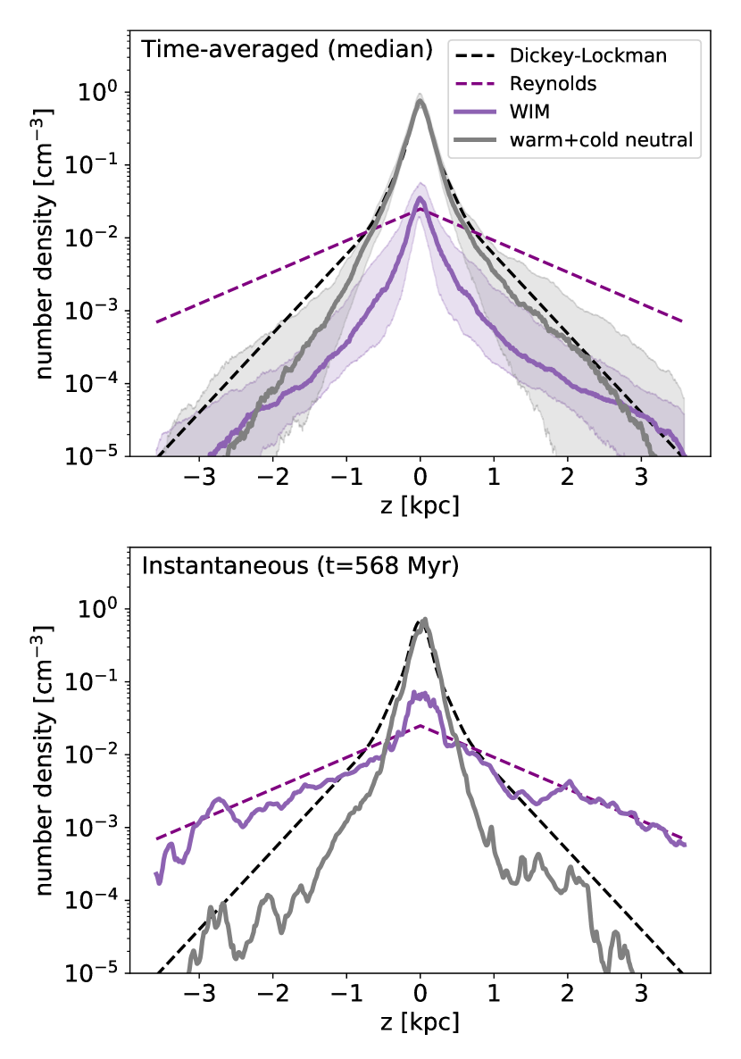
Figure 15: Comparison of vertical profiles of $n_{\rm H^{0}}$ (grey) and $n_{\rm e}$ (purple) from the simulation with Milky Way observations. The dashed lines show observed estimates of the Dickey-Lockman layer for the neutral hydrogen (see Equation 11) and the Reynolds layer for free electrons (see Equation 12). The solid curves show the mean (top) and instantaneous (bottom, at $t=568\,{\rm Myr}$) TIGRESS $n_{\rm e}$ and $n_{\rm H^{0}}{}$ vertical profiles. Shaded regions in the top panel indicate 25^thand 75^thpercentile range.

Based on various surveys of $21\,{\rm cm}$ emission from neutral atomic hydrogen, McKee et al. (2015) estimated that the vertical distribution of H I in the solar neighborhood follows

$$\dfrac{\langle n_{\rm H^{0}}\rangle_{\rm D\mbox{-}L}}{{\rm cm}^{-3}} =0.47e^{-\tfrac{1}{2}\left(\tfrac{z}{90\,{\rm pc}}\right)^{2}}+0.13e^{-\tfrac{1}{2}\left(\tfrac{z}{225\,{\rm pc}}\right)^{2}}$$

$$\mathrel{\phantom{=}}{}+0.077e^{-\left(\tfrac{|z|}{403\,{\rm pc}}\right)}\,,$$ (11)

where the two Gaussian components represent warm-cold H I in the main disk and the exponential component accounts for an extended layer at high altitudes. This “Dickey-Lockman” profile is shown as black dashed lines in Figure 15.

The DM of pulsars with known distances provides a direct measure of the WIM content in the Milky Way. The ratio between DM and the pulsar distance indicates the line-of-sight average electron densities of $\sim 0.01$–$0.1\,{\rm cm}^{-3}$ for pulsars with $|z|\lesssim 1\,{\rm kpc}$, with the vertical component of DM saturating at ${\rm DM}_{\perp}\sim 25\,{\rm pc}\,{\rm cm}^{-3}$ for pulsars at $|z|>1\,{\rm kpc}$ (e.g., Reynolds, 1991a; Gaensler et al., 2008; Schnitzeler, 2012; Deller et al., 2019). A number of studies found that an exponential disk with (extrapolated) midplane density $\langle n_{\rm e,0}\rangle\sim 0.01$–$0.03\,{\rm cm}^{-3}$ and scale height $h(n_{e})\sim 1\,{\rm kpc}$ reasonably accords with observations. The dashed purple lines in Figure 15 show the widely adopted form

$$\langle n_{\rm e}\rangle_{\rm R}=0.025\exp(-|z|/1\,{\rm kpc})\,{\rm cm}^{-3}$$ (12)

for the Reynolds layer. Note that based on current observed estimates, the WIM begins to dominate over H I for $|z|\gtrsim 700\,{\rm pc}$.

The top panel of Figure 15 shows that that the time-averaged TIGRESS profile (solid grey curve) matches the observed Dickey-Lockman profile for neutral gas quite well out to $|z|=3\,{\rm kpc}$ (i.e. the observed profile lies within the 25^th-75^th percentile range of the TIGRESS profile). As shown for example in the lower panel of Figure 15, individual instantaneous snapshots also agree quite well with the observed Dickey-Lockman profile within $|z|<500\,{\rm pc}$ (median of the logarithmic residual $\log_{10}(\langle n_{\rm H^{0}}\rangle/\langle n_{\rm H^{0}}\rangle_{\rm D\mbox{-}L})$ is $0.11$). At larger $|z|$, there is more variation in time, as indicated by the grey shaded region in the top panel.

In the top panel of Figure 15, the time-averaged median profile of the WIM from our simulation is shown by the solid purple curve (the shaded region again shows the 25^th-75^th percentile region). Clearly, the normalization of our mean WIM profile at large $|z|$ is well below the observational estimate of the Reynolds layer (dashed purple line), although the slope of our WIM profile at heights $|z|\gtrsim 1\,{\rm kpc}$ becomes shallower than that of the total warm gas, which is in agreement with observations. In order for the vertical profile of warm ionized gas to be significantly shallower than that of the total warm gas, the ionization fraction of warm gas must rise as a function of distance from the midplane – indeed, this is shown in panel (e) of Figure 7.

Though the properties of the observed Reynolds layer are not reproduced by the time-averaged WIM profile in our simulation, we note that profiles quite similar to Equation 12 are recovered in a minority of snapshots. An example is shown in the lower panel of Figure 15.

4.2.1 Potential Explanations for Discrepancies with Observations

One can think of two possible reasons that can explain the discrepancy between our median WIM profile and the observational estimate: (1) lack of ionizing photons and (2) lack of high-altitude gas to be ionized. Regarding the first possibility, massive stars in the TIGRESS simulation produce enough photons to maintain the ionization of the Reynolds layer. For a clumpy WIM disk with an exponential scale height $h$ and a constant volume filling fraction $f_{V,{\rm WIM}}$, the minimum ionizing photon rate per unit area required to balance the total recombination is $\Phi_{\rm i,min}=\alpha_{\rm B}\langle n_{\rm e,0}\rangle^{2}h/f_{V,{\rm WIM}}$, where $\langle n_{\rm e,0}\rangle$ is the area-averaged electron number density at $z=0$. Adopting $f_{V,{\rm WIM}}=0.1$ (e.g., Berkhuijsen & Müller, 2008) and $\langle n_{\rm e,0}\rangle=0.025\,{\rm cm}^{-3}$ (Equation 12), the ionization of the Reynolds layer requires $\Phi_{\rm i,min,R}=4.8\times 10^{49}\,{\rm s}^{-1}\,{\rm kpc}^{-2}$. This adopted value of $f_{V,\rm WIM}$ yields (obtained by integrating Equation 12) ${\rm EM}=n_{\rm e,0}^{2}h/(2f_{V,\rm WIM})=3.12\,{\rm pc}{}\,{\rm cm}^{-6}$. This is within a factor of two of the measurement of Hill et al. (2008), who find an emission measure of $1.406\pm 0.004\,{\rm pc}{}\,{\rm cm}^{-6}$. Row (a) in Figure 4 shows that most (90%) of the TIGRESS snapshots have sufficient ionizing photon production rate to ionize the Reynolds layer. In fact, a large fraction of snapshots (56%) have $\Phi_{\rm i}$ that is high enough to fully ionize even the smooth Dickey-Lockman layer, $\Phi_{\rm i,min,D\mbox{-}L}=3.4\times 10^{50}\,{\rm s}^{-1}\,{\rm kpc}^{-2}$.

Since the real gas distribution is clumpy and dense gas is highly correlated with ionizing sources, however, the majority of ionizing photons are absorbed by gas and dust near ionizing sources and the number of ionizing photons escaping into the diffuse ISM is greatly reduced. For example, we find that the mean value of ionizing photon flux passing through the planes $z=\pm 200\,{\rm pc}$ ($\Phi_{\rm i,|z|=200\,{\rm pc}}$) is only $2.3\times 10^{49}\,{\rm s}^{-1}\,{\rm kpc}^{-2}$, which is only 6% of time-averaged median $\Phi_{\rm i}$. Only 22% of snapshots satisfy $\Phi_{\rm i,|z|=200\,{\rm pc}}>3.2\times 10^{49}\,{\rm s}^{-1}\,{\rm kpc}^{-2}$, which would be the minimum required to maintain the ionization profile described by Equation 12 at $|z|>200\,{\rm pc}$.

H II region dynamics (not included in the current simulations) are likely to aid the escape of radiation from star-forming clouds, so that a larger proportion of $\Phi_{\rm i}$ would emerge from the midplane than we have found. Recent numerical simulations of individual molecular clouds have shown that radiation feedback from massive stars plays a key role in driving gas dispersal on the scale of tens of parsecs (e.g., Walch et al., 2012; Dale et al., 2012, 2013; Kim et al., 2018; Haid et al., 2019; He et al., 2019; Kimm et al., 2019; González-Samaniego & Vazquez-Semadeni, 2020). In particular, Kim et al. (2019) showed that a significant fraction of ionizing photons escape on a short timescale ($\lesssim 3\,{\rm Myr}$) through low-density channels created by stellar feedback and turbulence, which can boost the photon budget to ionize DIG.

In addition to a lack of photons, and perhaps more importantly, we believe that the discrepancy between our median WIM profile and the observational estimate is caused by the fact that there is simply not enough material to be ionized at large $|z|$: the mean profile of $\langle n_{\rm H}\rangle$ from our simulation is lower than the observational constraints by a factor $3$–$5$ at $1$–$2\,{\rm kpc}$. One possible reason for this discrepancy is that the TIGRESS simulation underestimates outflows, potentially because effects of cosmic rays have not been included. A second possibility is that inflowing extragalactic gas, not captured in TIGRESS, is responsible for most of the extended WIM. In Section 3.7, we previously noted that the deficit of blueshifted ${\rm H}\alpha$  in our synthetic profile (compared to WHAM) could potentially be due to missing extragalactic inflow.

It is also possible that the present state of the DIG in the local Milky Way is atypical. Indeed, although the ionized gas content is insufficient to match the observations for the majority of snapshots, we find that a small fraction of snapshots have vertical profiles that are in good agreement with observational constraints. For example, snapshots at $t\sim 550$–$570\,{\rm Myr}$ have substantial amounts of warm fountain gas at high altitudes lifted up by SN feedback from previous generation of star formation. The ongoing star formation produces sufficient photons, and channels are available for their escape, such that an extended DIG layer comparable to the observed Reynolds layer is present. Profiles from a snapshot at time $t=568\,{\rm Myr}$ shown in the bottom panel of Figure 15 is an example of such case. (see also Figure 3).

Lastly, it has long been suggested that runaway OB stars may act as effective ionization source of DIG (e.g. Heiles & Kulkarni, 1987; Rand, 1993). Runaways stars are flung at high speeds from their birthplace by dynamical encounters in dense stellar systems (e.g., Poveda et al., 1967; Fujii & Portegies Zwart, 2011) or by explosion of a companion star in a binary system (e.g., Blaauw, 1961; Portegies Zwart, 2000)). Once they move to high-altitude, low-density regions, ionizing photons emitted by these runaways would more easily escape the galaxy and ionize warm neutral gas along the way (e.g., Conroy & Kratter, 2012).

We find that runaways that represent binary companions have a negligible impact on the ionization state, as shown in Appendix A. However, we caution that the ionizing photon rate that we used is likely an underestimate because all of runaways modeled in our simulation are secondaries in binary systems, which are mostly B-type (or late O-type) stars. Dynamically ejected runaways are likely to be younger and more massive than binary runaways and produce more ionizing photons. We also note that our approach to calculating the rate of ionizing photons from runaways is not internally consistent because the SN rate as well as the mass-luminosity relation are taken from stellar evolution and population synthesis models containing only single stars (Leitherer et al., 1999; Bruzual & Charlot, 2003). If the effects of binary interaction is included, the ionizing photon rate at late stage of stellar evolution could be boosted by several orders of magnitude (e.g., Götberg et al., 2019).

4.3 Comparison with Observations: the WIM scale height

We measure a time-averaged mean scale height of the warm ionized gas $H_{\rm w,i}=556\pm 186\,{\rm pc}$. This mean value is in good agreement with some observed measurements of the Milky Way WIM, allowing for typical uncertainties of $\sim 100$–$200$ pc (Nordgren et al. 1992 measure a scale height of 670 pc, while Peterson & Webber 2002 find a scale height of 830 pc). However, many empirical estimates of the average WIM scale height are larger: Taylor & Cordes 1993, Savage et al. 1990, Reynolds 1991b, and Berkhuijsen & Müller 2008 give a scale height of $\sim 900$ pc, while Gómez et al. 2001 measures a scale height of $\sim 1100$ pc, and Gaensler et al. 2008 measures a scale height of $\sim 1800$ pc. The possible reasons given above for our discrepancy with the overall “Reynolds” profile could potentially also explain why our measured WIM scale height is smaller than most empirical estimates.

Under the simplistic assumption that a sample of Milky Way-like galaxies should be similar to the ensemble obtained via evolution of the TIGRESS box, our results on the distribution of ${\rm H}\alpha$ scale height (as presented in Figure 9) can be compared to scale height measurements in nearby disk galaxies. The scale height of the DIG in an external galaxy is measured significantly differently from internal scale height measurements of the Milky Way, both due to constraints on the nature of data collected (via ${\rm H}\alpha$ in integral field unit spectroscopy or narrowband imaging) and due to technical constraints (e.g., the influence of the point spread function on the observed scale height). To account for this, we also compute scale heights wherein an exponential profile is fit to the $n_{\rm e}^{2}$ vertical profile at $|z|>1\,{\rm kpc}$ (see Section 3.4).

We find that our distribution of ${\rm H}\alpha$ scale heights is generally similar to observed distributions, but because we have not attempted to simulate the effects of the point spread function (PSF, which often have extended low surface brightness wings), because our simulation aims to reproduce only Solar Neighborhood conditions and because samples of ${\rm H}\alpha$ scale heights remain relatively small, we cannot make a strict statement of (in)consistency from this comparison.

We find a median exponential-fit $n_{\rm e}^{2}$ scale height of $0.44^{+0.33}_{-0.15}\,{\rm kpc}$, here reporting the inner 68% of the distribution in order to compare to literature observations. The distribution of measured ${\rm H}\alpha$ scale heights for a sample of edge-on disk galaxies presented in Levy et al. (2019) find a median scale height of $0.8^{+0.7}_{-0.4}\,{\rm kpc}$, with the maximum likelihood scale height at $\sim 0.5\,{\rm kpc}$ and an extended tail towards scale heights of larger than $1\,{\rm kpc}$, much like our distribution of exponential-fit scale heights in Figure 9. Bizyaev et al. (2017) find a somewhat higher median ${\rm H}\alpha$ scale height of $1.2\pm 0.5\,{\rm kpc}$ for a sample of 67 edge-on galaxies observed by MaNGA. Finally, Jo et al. (2018) observes a mean ${\rm H}\alpha$ scale of $430\pm 50\,{\rm pc}$ for a sample of edge-on galaxies at $d_{L}\lesssim 25$ Mpc, comparable to the mean of the distribution of our exponential-fit scale heights ($535.4\pm 10.\,{\rm pc}$).

As previously shown in Section 3.4, we find no strong temporal correlation between the global SFR density of the simulation and the exponential-fit $n_{\rm e}^{2}$ scale height. In the literature, a positive correlation has been reported between ${\rm H}\alpha$ luminosity and ${\rm H}\alpha$ scale height (Bizyaev et al., 2017), while a weak anticorrelation has been reported between the extraplanar midplane EM and the ${\rm H}\alpha$ scale height (Miller & Veilleux, 2003). We again however emphasize that our simulations are initialized with Solar neighborhood-like conditions, and cannot be interpreted as direct analogs to external galaxy samples which may have a wider range of conditions than presented by the time-varying state in our single TIGRESS simulation.

4.4 The Clumping Correction Factor

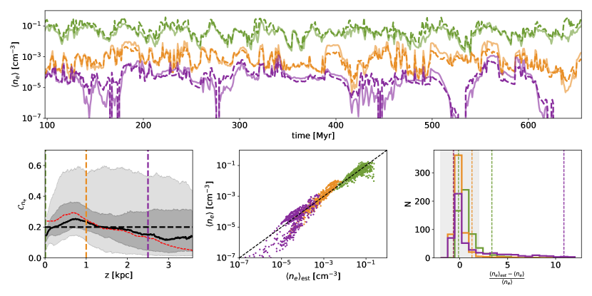
Figure 16: Top: the time evolution of the average $n_{\rm e}$ at the midplane (green), $1\,{\rm kpc}$ above the midplane (orange), and $2.5\,{\rm kpc}$ above the midplane (purple). For each, the solid curves show the true values of $\langle n_{\rm e}\rangle$ and the dashed curves show the estimated average $\langle n_{\rm e}\rangle_{\rm est}$ using the observable $\langle n_{e}^{2}\rangle$ and the height-averaged, time-averaged median clumping correction factor, $C_{n_{\rm e}}^{50}=0.2$. Bottom Left: the clumping correction factor as a function of height, $C_{n_{\rm e}}(z)$ (as given by Equation 15). The solid black curve shows the time-averaged median value of the clumping correction factor, while the dashed horizontal line shows the time-averaged, height-averaged median value of the clumping correction factor. The grey shaded regions show the 25^th to 75^th and 5^th to 95^th percentile regions. The colored dashed lines show the heights that correspond to the time evolution plot at top. We also show the median profile of the square root of the warm ionized volume filling factor, $f_{V,\rm WIM}^{1/2}$, with a red dashed curve. In the idealized case of constant $n_{\rm e}$ within fully-ionized portions of the volume, $C_{n_{\rm e}{}}=f_{V,\rm WIM}^{1/2}$. Bottom Middle: the relation between estimated electron density ($\langle n_{\rm e}\rangle_{\rm est}$) and the true $\langle n_{\rm e}\rangle$, colored by height. Bottom Right: the distribution of fractional error incurred by estimating $\langle n_{\rm e}\rangle$ using the time-averaged, height-averaged median value of the clumping correction factor. The grey shaded region is bounded by [-2,2]. The histograms show the fractional error distribution at the midplane (green), $1\,{\rm kpc}$ (orange), and $2.5\,{\rm kpc}$ (purple). The dashed vertical lines show the 5^th and 95^th percentiles of the distribution for each of the heights above.

${\rm H}\alpha$ observations of edge-on disk galaxies have been used to infer the physical properties of the DIG such as electron density and total mass/column density (e.g., Dettmar, 1990; Rossa & Dettmar, 2000; Boettcher et al., 2019). Because the ${\rm H}\alpha$ surface brightness (or EM) is proportional to the integral of squared electron density along the line of sight, however, deriving these quantities from the EM requires a knowledge of the spatial distribution of ionized gas as well as the effective path length through the galaxy. Simulations allow us to directly measure the “clumping correction factor” needed to convert EM into electron density. In addition to providing a calibration, simulations also allow us to gauge the uncertainties incurred by assuming a constant value of the clumping correction factor in a dynamic and varying system.

Here, we compute the clumping correction factor of DIG as a function of $z$, and use this as a multiplicative factor to determine the value of the (line-of-sight averaged) electron density from an observed EM. We also provide a simple analytic expression for the effective path length in terms of disk scale length and local radius. These results are intended to aid in obtaining estimates and expected errors for the content of the DIG based on observations of external galaxies.

We define the clumping correction factor at height $z$ as

$$\mathcal{C}_{n_{\rm e}} \equiv\sqrt{\dfrac{(\int n_{\rm e}\Theta_{\rm w}dA/A)^{2}}{\int n_{\rm e}^{2}\Theta_{\rm w}dA/A}}$$ (13)

$$=\sqrt{\frac{{\langle{n_{\rm e}}\rangle}^{2}}{{\langle{n_{\rm e}^{2}}\rangle}}}\,,$$ (14)

where the brackets $\langle\rangle$ denote the $x$-$y$ area average and $\Theta_{\rm w}{}$ is a top hat function that filters warm gas with $5\times 10^{3}\,{\rm K}<T<2\times 10^{4}\,{\rm K}$. In the idealized case where all WIM clouds are fully ionized and have the same electron density, the clumping correction factor and volume filling factor at a given height are related: $\mathcal{C}_{n_{\rm e}}=f_{V,{\rm WIM}}^{1/2}$, where $f_{V,{\rm WIM}}=\int x_{\rm i}\Theta_{\rm w}dA/A$.

From our simulations, we compute statistics of the clumping correction factor ${\mathcal{C}}_{n_{\rm e}}$ as a function of height off the midplane ($z$) and time. ${\mathcal{C}}_{n_{\rm e}}$ may then be used with a known value of $\langle n_{\rm e}^{2}\rangle$ to predict the area-averaged mean electron density at $z$. Let us define the instantaneous average of EM over the local radial direction ($x$) in the plane of the sky at height $z$ as ${\langle{{\rm EM(z)}}\rangle_{x}}\equiv\int n_{\rm e}^{2}dxdy/L_{x}=\langle n_{\rm e}^{2}\rangle L_{y}$. Then, from Equation 14 we have

$$\langle n_{\rm e}\rangle_{\rm est}(z)=\mathcal{C}_{n_{\rm e}}(z)\sqrt{\dfrac{{\langle{\rm EM(z)}\rangle_{x}}}{L_{y}}}\,.$$ (15)

The bottom-left panel of Figure 16 shows the time-averaged median of $\mathcal{C}_{n_{\rm e}}(z)$ from our simulation, as well as the 25^th to 75^th and 5^th to 95^th percentiles. Evidently, $\mathcal{C}_{n_{\rm e}}(z)$ is largely constant as a function of $z$, with an overall (time-averaged, height-averaged) median value of $C_{n_{\rm e}{}}^{50}=0.2$ (and a 25^th and 75^th percentile value of $C_{n_{\rm e}}^{25}=0.11$ and $C_{n_{\rm e}}^{75}=0.31$). We also find that the clumping correction factor does not vary significantly with electron density or total gas density. We show the application of this clumping correction factor as a function of time for gas at the midplane (green), $1\,{\rm kpc}$ (orange), and $2.5\,{\rm kpc}$ (purple) in the top panel of Figure 16. Here, the solid curves show the true value of $\langle n_{\rm e}\rangle$ and the dashed curves show the estimated value $\langle n_{\rm e}\rangle_{\rm est}$ using the constant calibration factor of $\mathcal{C}_{n_{\rm e}}^{50}=0.2$.

Using this median value in Equation 15, the bottom-middle panel of Figure 16 compares the actual $\langle n_{\rm e}\rangle$ with the estimated value for all snapshots at $z=0,1,2.5\,{\rm kpc}$, colored by height. The distribution of fractional error is then shown in the bottom-right panel of Figure 16. This shows that using a time-averaged, height-averaged median value of $\mathcal{C}_{n_{\rm e}}=0.2$ we can successfully convert from $\langle n_{\rm e}^{2}\rangle$ to $\langle n_{\rm e}\rangle$ within a factor of 2 for 95% of snapshots at $|z|\sim 1\,{\rm kpc}$.

For application to observed galaxies, we suppose that an observer wants to make an estimate of the local electron density of DIG along the line of sight in an edge-on galaxy, such that the plane of the sky is the $x$-$z$ plane ($x$ is the local radial direction). To apply Equation 15, the known $L_{y}$ in the simulation must be replaced with ${\cal\ell}_{y}$, an effective path length along the line of sight.

To illustrate the idea, let us assume that the electron density $\tilde{n}_{\rm e}$, averaged over a small volume (but sufficiently representative of the local condition), is an exponential function of the galactocentric radius $\tilde{n}_{\rm e}(R,z)=\tilde{n}_{\rm e,0}(z)e^{-R/R_{d}}$, where $R_{d}$ is the radial scale length. If the clumping correction factor $\mathcal{C}_{n_{\rm e}}$ does not vary with $R$, the EM at some (projected) galactocentric radius $R$ and at some height $z$ can be written as

$${\rm EM}(R,z) =\int_{-\infty}^{\infty}\mathcal{C}_{n_{\rm e}}^{-2}\tilde{n}_{\rm e,0}^{2}(z)e^{-\frac{2}{R_{d}}\sqrt{R^{2}+y^{2}}}dy$$ (16)

$$\equiv\mathcal{C}_{n_{\rm e}}^{-2}\tilde{n}_{\rm e}^{2}(R,z)\ell_{y}$$ (17)

where the effective path length $\ell_{y}=2R\int_{0}^{\infty}e^{-q\sqrt{1+s^{2}}}ds$ with $q=2R/R_{d}$. The integral can be approximated as

$$\int_{0}^{\infty}e^{-q\sqrt{1+s^{2}}}ds\approx\frac{e^{-q}(1+q)}{q(1+0.2q)}\,,$$ (18)

which is accurate to within $\sim 10\%$ for $q<10$. The estimate of electron density is then

$$\tilde{n}_{\rm e}(R,z)\approx\mathcal{C}_{n_{\rm e}}\left(\frac{{\rm EM}(R,z)}{R_{d}}\right)^{\frac{1}{2}}\left(\frac{1+0.4\frac{R}{R_{d}}}{1+\frac{2R}{R_{d}}}\right)^{\frac{1}{2}}e^{R/R_{d}}$$ (19)

for the adopted value of $\mathcal{C}_{n_{\rm e}{}}$. In practice, $R_{d}$ can be estimated from the ${\rm H}\alpha$ scale length of the disk, i.e., $R_{d}=2R_{{\rm H}\alpha}$. While the measured EM (or ${\rm H}\alpha$ surface brightness) would be a weighted average of ${\rm EM}(R,z)$ over a finite area due to PSF effects, for spatially resolved edge-on galaxies Equation 19 would provide a reasonably good estimate of the density of DIG.

Berkhuijsen & Müller (2008) estimated a volume filling factor of the WIM $f_{V,{\rm WIM}}\sim 0.1$, based on EM and DM to pulsars with distances known within $50\%$ and assuming uniform $n_{e}$. The implied clumping correction factor would then be $\mathcal{C}_{n_{\rm e}}=0.3$, slightly larger than the value obtained from our simulation. Finally, we note that although $\mathcal{C}_{n_{\rm e}}$ is identically equal to $(f_{V,{\rm WIM}})^{1/2}$ only in the case of constant $n_{\rm e}$ in fully-ionized regions, we find that these quantities are in fact quite close to each other. In Figure 7(b), we presented the median WIM volume filling factor; in the lower-left panel of Figure 16 we now overplot the square root of this in red.

5 Summary

In this study, we have applied radiation-transfer post-processing to TIGRESS MHD simulation outputs in order to study the properties of the WIM. The sources of ionizing (and FUV) photons for the radiative transfer are star particles that have formed as a result of self-gravitating collapse. To our knowledge, this is the first such radiative transfer model in which star formation, SN rates and locations, the (global) FUV heating rate, and the properties of ionizing sources are self-consistently determined. With a self-consistent spatio-temporal correlation of SNe and ISM gas, the overall vertical distribution of warm gas and the network of porous (hot ISM) channels that allow photons to propagate over kpc scales are more realistic than in previous work, and the photon input rate is set by the time-varying star formation rate rather than being a free parameter.

The TIGRESS model that we consider represents a galactic environment similar to the local Milky Way. The median ionizing photon production rate is $\Phi_{\rm i}=4.0\times 10^{50}\,{\rm s}^{-1}\,{\rm kpc}^{-2}$, although this varies significantly as only $\sim 3$ sources account for 90% of the ionizing photons at any one time (see Figure 5). The mean escape fraction of ionizing photons from the galaxy is only $1.1\%$; A much larger fraction ($\sim 22\%$) of non-ionizing photons escape from the galaxy (Figure 4c).

Most of the ionizing photons are absorbed by dense gas ($n_{\rm H}>1\,{\rm cm}^{-3}$) near the midplane. Overall, approximately half of ionizing photons are absorbed by neutral hydrogen and half by dust (Figure 4d); absorption by neutral hydrogen is completely dominant at high $|z|$ where the ionization parameter is low ($U=10^{-5}-10^{-3}$, see Figure 6).

Nevertheless, diffuse warm ionized gas is abundant far from the midplane, with $40\%$ of the ionized gas mass found at $|z|>200\,{\rm pc}$, and a peak in the WIM volume filling factor at $|z|\sim 0.5-0.8\,{\rm kpc}$ (Figure 7 (c) and (b), respectively). The proportion of warm gas that is ionized increases with $|z|$ (Figure 7(f)). There is a positive correlation between volume filling factor of ionized gas and SFR (Figure 8).

To make a quantitative comparison to observations, we fit the high-$|z|$ ($>1\,{\rm kpc}$) EM to an exponential. Our simulation shows large temporal variability in this exponential-fit scale height, with a typical value of $h(n_{\rm e}^{2})\sim 400\,{\rm pc}$ and a tail that extends up to $\sim 2$ kpc (Figure 9). This is comparable to estimates of the DIG scale height in both the Milky Way and external edge-on galaxies, though small observational sample sizes and the applicability of Solar Neighborhood conditions to those samples make a direct comparison uncertain.

Our simulations also allow us to assess the “clumping” of ionized gas. At $|z|>200\,{\rm pc}$, most of the ${\rm H}\alpha$ emission is from ionized gas clouds with local density $0.1$-$1\,{\rm cm}^{-3}$ (Figure 10), although the horizontal average $\langle n_{\rm e}\rangle$ and the “typical” $n_{e}=\langle n_{\rm e}\rangle/f_{V,{\rm WIM}}$ are much lower (panels (c) and (d), respectively, of Figure 7).

We find that the mean (volume-averaged) electron density in the DIG is related to the mean value of the square of the electron density by $\langle n_{\rm e}\rangle=\mathcal{C}_{n_{\rm e}}\sqrt{\langle n_{\rm e}^{2}\rangle}$ for $\mathcal{C}_{n_{\rm e}}\sim 0.2$ (see Section 4.4). In our simulations, this clumping calibration factor is remarkably independent of time and of height above the midplane. The numerical calibration of clumping should be useful in converting EM from observations of ${\rm H}\alpha$ surface brightness (or other WIM tracers) in edge-on galaxies to mean density of the DIG. For the case of disk with density declining exponentially with radius, we give an approximate prescription for obtaining $n_{\rm e}{}(R,z)$ from $EM(R,z)$, the exponential scale length $R_{d}$, and the distance $R$ from the center of the galaxy (Equation 19).

When observed “face-on” (along the z-axis), the EM distribution of the WIM in the disk is centered on $\sim 0.1\,{\rm pc}\,{\rm cm}^{-3}$ (see Figure 11), though the breadth of the distribution increases for smaller effective beam size (Figure 12). Overall, even though nearly half of ionized gas in our simulations comes from high-altitude regions ($|z|>200\,{\rm pc}$), only $\sim 5\%$ of the ${\rm H}\alpha$ emission is produced there, due to the low gas density.

In comparing our synthetic line profiles to WHAM observations, we find that the shape and normalization of the time-averaged redshifted (outflowing) side matches well, but that the simulation does not produce sufficient ${\rm H}\alpha$ emission at blueshifted velocities (inflowing, see Figure 13). We also find that the mean electron density inferred from DM of pulsars at high $|z|\sim\,{\rm kpc}{}$ significantly exceeds the level in our simulations (Figure 15). Taken together, this raises the intriguing possibility that much of the Reynolds layer is an ionized extragalactic inflow. An alternative possibility, of course, is that the TIGRESS simulations have significantly underestimated the mass involved in fountain flows, and at the current time the fountain is mostly in an inflow episode. However, our mean profiles of neutral gas match the Dickey-Lockman profile inferred from 21 cm out to $\sim 3\,{\rm kpc}$ (Figure 15). We also note that for some individual epochs in our simulation, the instantaneous $n_{e}(z)$ profile matches that inferred from pulsar DM very well (as discussed in Section 4.2).

The high-velocity portions of our synthetic ${\rm H}\alpha$ profiles are exponential (Figure 13), consistent with the underlying exponential distribution of mass with velocity in extraplanar “fountain” gas. At most times in our models, more than half of the high-velocity (defined as $|v|>50\,{\rm km}\,{\rm s}^{-1}$) ionized gas is located at high altitudes (Figure 14). In cases where the ${\rm H}\alpha$ wing emission at $v>50\,{\rm km}\,{\rm s}^{-1}$ exceeds $\sim$2% of the total ${\rm H}\alpha$ emission, the majority of the wing emission originates from high-altitude gas. Periods of stronger wing emission correspond to strong outflows, and are time-delayed relative to strong bursts of star formation.

Finally, we remark that while the present study offers a significant advance over previous work, it is not without limitations. In particular, the ionization state is computed via post-processing, where for each snapshot, we evolve until ionization equilibrium is reached. In reality, for low-density, high-altitude regions, the radiation field (or source visibility) may change more rapidly than the recombination rate, so that the true ionization level may be higher than we estimate. For simplicity, we have adopted a constant temperature for the ionized gas, but to make more comparisons with multi-line observations heating and cooling of ionized gas must be included self-consistently. Inclusion of cosmic rays that dynamically interact with the gas could potentially enhance the mass of gas in the extraplanar region. As mentioned in Section 4.2.1, resolving cloud-scale feedback processes before the first SNe could increase the fraction of ionizing photons escaping into the diffuse ISM. In the future, it will be valuable to include time-dependent radiative transfer and adaptive mesh refinement as part of the MHD simulation.

The present study deals only with Solar neighborhood-like conditions. It is also of interest for the future to extend the same kind of analysis to other galactic environments; simulations with conditions representative of galactic centers and disk outskirts will allow for fuller predictions of the state of DIG in disk galaxies.

Appendix A Effect of Runaways

Binary runaway OB stars ejected from stellar clusters after a supernova can, in principle, act as sources of ionizing radiation at large distances from the disk (see Figure 2, leftmost panel). Because TIGRESS tracks such runaways, we can examine whether such stars make a significant contribution to the DIG. The main sequence lifetime of each runaway is chosen to be consistent with the specific SNe rate (bottom panel, Figure 1) – a full description of the prescription for this assignment is given in Kim & Ostriker (2017). The ionizing photon luminosity of a runaway is then computed from its main sequence lifetime using the main sequence lifetime-mass and mass-luminosity relations given in Parravano et al. (2003). Since the EUV luminosity drops to relatively negligible levels at $t>10\,{\rm Myr}$, we consider a maximum of 20 brightest runaways as sources of ionizing radiation simultaneously. For most of snapshots, this accounts for more than 90% of the total ionizing photon rate of all runaways.

In Figure 17, we show diagnostics of the effect of runaways on the ionizing photon rate in the simulation box and structure of the WIM. In the left panel, the grey curve show the ionizing photon rate per unit area when runaways are not considered as ionizing sources, while the red curve show the results when runaways are included as sources of ionizing radiation. The right panel shows the ionizing photon rate for clusters versus that from runaways for each snapshot. The median ionizing photon rate from runaways is 1.7% that of clusters – though the rate of ionizing photons from runaways is as high as that from clusters in 3% of snapshots, the overall contribution of runaways to the ionizing photon rate is smaller than that of clusters by several orders of magnitude.

The effect of runaways is small relative to the variation in time, and does not induce a significant systematic change in the structure of the DIG. We find that the inclusion of runaways induces a change in the area-averaged WIM electron density that is small compared to the fluctuations we observe due to time evolution, as shown in the left panel of Figure 17. Thus, we choose to exclude runaways as sources of ionizing radiation for this work.

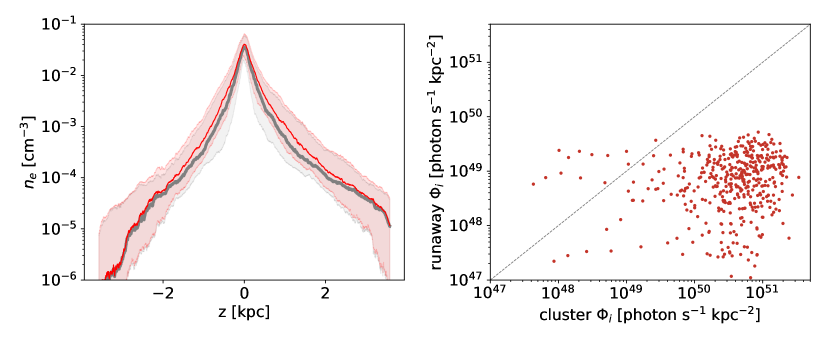
Figure 17: Left: Time-averaged $n_{\rm e}{}$ vertical profiles when the contribution of runaways is included (red) and when runaways are neglected (grey). As in Figure 7, the solid curves show the median profile, while the shaded regions show the 25^th and 75^th percentiles. Right: the specific ionizing photon rate $\Phi_{\rm i}$ of clusters versus $\Phi_{\rm i}$ from runaways. For most snapshots, runaways contribute about 1% as many ionizing photons as clusters.

References

- jon (2001) 2001, SciPy: Open source scientific tools for Python, ,
- Abbott (1982) Abbott, D. C. 1982, ApJ, 263, 723
- Altay & Theuns (2013) Altay, G., & Theuns, T. 2013, MNRAS, 434, 748
- Astropy Collaboration et al. (2013) Astropy Collaboration, Robitaille, T. P., Tollerud, E. J., et al. 2013, A&A, 558, A33
- Barnes et al. (2014) Barnes, J. E., Wood, K., Hill, A. S., & Haffner, L. M. 2014, MNRAS, 440, 3027
- Barnes et al. (2015) —. 2015, MNRAS, 447, 559
- Berkhuijsen & Fletcher (2015) Berkhuijsen, E. M., & Fletcher, A. 2015, MNRAS, 448, 2469
- Berkhuijsen et al. (2006) Berkhuijsen, E. M., Mitra, D., & Mueller, P. 2006, Astronomische Nachrichten, 327, 82