Characterizing Quantum Networks: Insights from Coherence Theory

Abstract

Networks based on entangled quantum systems enable interesting applications in quantum information processing and the understanding of the resulting quantum correlations is essential for advancing the technology. We show that the theory of quantum coherence provides powerful tools for analyzing this problem. For that, we demonstrate that a recently proposed approach to network correlations based on covariance matrices can be improved and analytically evaluated for the most important cases.

Introduction.— Quantum networks Kimble (2008); Sangouard et al. (2011); Simon (2017); Wehner et al. (2018) have recently attracted much interest as they have been identified as a promising platform for quantum information processing, such as long-distance quantum communication Cirac et al. (1998); Gisin et al. (2002). In an abstract sense, a quantum network consists of several sources, which distribute entangled quantum states to spatially separated nodes, then the quantum information is processed locally in these nodes. This may be seen as a generalization of a classical causal model Spirtes et al. (2000); Pearl (2009), where the shared classical information between the nodes is replaced by quantum states. Clearly, it is important to understand the quantum correlations that arise in such a quantum network. Recent developments have shown that the network structure and topology leads to novel notions of nonlocality Renou et al. (2019a); Gisin et al. (2020), as well as new concepts of entanglement and separability Navascues et al. (2020); Kraft et al. (2020); Luo (2020), which differ from the traditional concepts and definitions Acín et al. (2001); Gühne and Tóth (2009). Dealing with these new concepts requires theoretical tools for their analysis. So far, examples of entanglement criteria for the network scenario have been derived using the mutual information Navascues et al. (2020); Kraft et al. (2020), the fidelity with pure states Kraft et al. (2020); Luo (2020), or covariance matrices build from measurement probabilities Kela et al. (2020); Åberg et al. (2020), but these ideas work either only for specific examples, or require numerical optimizations for their evaluation.

In this paper we demonstrate that the theory of quantum coherence provides powerful tools for analyzing correlations in quantum networks. In recent years, quantum coherence was under intense research, it was demonstrated that coherence is essential in quantum information applications and entanglement generation Aberg (2006); Baumgratz et al. (2014); Killoran et al. (2016); Regula et al. (2018) and a resource theory of it has been developed Streltsov et al. (2017a); Chitambar and Gour (2019); Winter and Yang (2016); Chitambar and Hsieh (2016); Streltsov et al. (2017b). We provide a direct link between the theory of multisubspace coherence Ringbauer et al. (2018); Kraft and Piani (2019) and the approach to quantum networks using covariance matrices established in Refs. Kela et al. (2020); Åberg et al. (2020). This allows to solve analytically the criteria developed there for important cases; furthermore, some conjectures can be proved and, besides that, our methods can be applied to large networks for which tools based on numerical optimization are infeasible. We note that, since the covariance matrix approach is essentially a tool coming from classical causal models Kela et al. (2020), our results demonstrate that results from the theory of quantum coherence are useful beyond the level of quantum states for the analysis of classical networks.

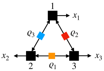
(a)

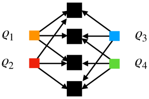
(b)

$\displaystyle\Gamma(\mathbf{v})=\matrixquantity(\color[rgb]{0,1,1}\blacksquare&\color[rgb]{0,1,1}\blacksquare&\phantom{\blacksquare}\\ \color[rgb]{0,1,1}\blacksquare&\color[rgb]{0,1,1}\blacksquare&\\ &&)_{3}+\matrixquantity(\color[rgb]{1,0,0}\blacksquare&\phantom{\blacksquare}&\color[rgb]{1,0,0}\blacksquare\\ &&\\ \color[rgb]{1,0,0}\blacksquare&&\color[rgb]{1,0,0}\blacksquare)_{2}+\matrixquantity(\phantom{\blacksquare}&&\\ &\color[rgb]{1,.5,0}\blacksquare&\color[rgb]{1,.5,0}\blacksquare\\ &\color[rgb]{1,.5,0}\blacksquare&\color[rgb]{1,.5,0}\blacksquare)_{1}$

(c)

Figure 1: (a) In its simplest scenario, the triangle network consists of three nodes that produce measurement outcomes $x_{1},\dots,x_{3}$ and three sources that distribute bipartite entanglement that is shared amongst the nodes. (b) A network consisting of four nodes that is 3-complete, i.e., it features four sources that distribute tripartite entanglement. (c) The covariance matrix of the triangle network has a $3\times 3$ block structure and consists of three terms, where $\quantity(\square)_{i}$ denotes those blocks that are contributed by the source $i$.

Quantum networks.— The simplest non-trivial network is the triangle network, where three nodes are mutually connected by three sources that prepare bipartite quantum states that are then subsequently shared with the nodes, see also Fig. 1a. More generally, one has $M$ sources, labelled by $m=1,2,\dots,M$ that independently produce quantum states $\varrho_{m}$, which are then distributed to $N$ nodes, labelled by $n=1,2,\dots,N$. For every source $m$ we denote by $\mathcal{C}_{m}$ the set of all connected nodes that have access to the state $\varrho_{m}$. The topology of the network captures the fact that not all vertices are connected to a single source, thus limiting the influence that each source can have on the different nodes.

In the simplest case, at each node a measurement is performed that is described by a POVM $\mathbf{A}^{(n)}=\{A_{x}^{(n)}\}_{x}$. The observed probability distribution over the outcomes reads

$$p(x_{1}\dots x_{N})=\tr[(A_{x_{1}}^{(1)}\otimes\cdots\otimes A_{x_{N}}^{(N)})\varrho_{1}\otimes\cdots\otimes\varrho_{M}].$$ (1)

The central question is whether a given probability distribution may originate from a network with a given topology. We note that the set of probability distributions that are compatible with a given network topology is non-convex and thus, in general, hard to characterize. One way to overcome this problem was put forward in Ref. (Åberg et al., 2020). The idea is to map the set of probability distributions compatible with the network to the space of covariance matrices, and then consider a convex relaxation of the problem.

For this purpose, a so-called feature map is defined that maps the outcomes $x_{n}$ at each vertex $n$ to a vector $\mathbf{v}_{x_{n}}^{(n)}\in\mathcal{V}_{n}$, where the $\mathcal{V}_{n}$ are some orthogonal vector spaces. Combining all the feature maps, one obtains a random vector $\mathbf{v}$ with components $\mathbf{v}_{x_{1}\dots,x_{N}}=\mathbf{v}_{x_{1}}^{(1)}+\cdots+\mathbf{v}_{x_{N}}^{(N)}$. The covariance matrix is then defined as

$$\Gamma(\mathbf{v})=E(\mathbf{v}\mathbf{v}^{\dagger})-E(\mathbf{v})E(\mathbf{v})^{\dagger}$$ (2)

with $E(\mathbf{v}\mathbf{v}^{\dagger})=\sum_{x_{1},\dots,x_{N}}\mathbf{v}_{x_{1},\dots,x_{N}}\mathbf{v}^{\dagger}_{x_{1},\dots,x_{N}}P(x_{1},\dots,x_{N})$ and $E(\mathbf{v})=\sum_{x_{1},\dots,x_{N}}\mathbf{v}_{x_{1},\dots,x_{N}}P(x_{1},\dots,x_{N})$. Due to the structure of $\mathbf{v}$, the covariance matrix has a natural block structure: $\Gamma$ is an $N\times N$ block matrix with blocks $\Gamma_{\alpha\beta}$, and each block is a $r\times r$ matrix, with $r$ being the dimension of $\mathcal{V}_{n}$. The standard covariance matrix formalism from mean values is a special instance of this notion, where one assigns to the outcomes $x_{n}$ just real numbers and hence takes the $\mathcal{V}_{n}$ to be one-dimensional. Here, however, we will assume that the feature map simply maps the outcome $x_{n}$ to $\ket{x_{n}}$, as for measurements with more than two outcomes the mean value contains less information in comparison with the probability distribution.

Covariance matrices and coherence.— The topology of the network imposes strong constraints on the structure of the covariance matrix. More precisely, the covariance matrix can be decomposed in a sum of positive matrices that have a certain block structure, corresponding to the sources Åberg et al. (2020); Kela et al. (2020). The verification of this structure is then an instance of a semidefinite program (SDP) (Boyd and Vandenberghe, 2004; Gärtner and Matoušek, 2012). For simplicity, we will restrict our attention in the following to $k$-complete networks. This means that all sources distribute their states to $k<N$ parties and all possible $k$-partite sources are being used, so we have $M={N\choose k}$ (see also Fig. 1b). Our results can be extended to more complicated network topologies.

The criterion from Refs. Åberg et al. (2020); Kela et al. (2020) states that one has to find a decomposition of $\Gamma(\mathbf{v})$ into blocks $Y_{m}$ according to

find: $$Y_{m}\geq 0$$ (3)

subject to: $$Y_{m}=\Pi_{m}Y_{m}\Pi_{m}\mbox{ and }\Gamma(\mathbf{v})=\sum_{m=1}^{M}Y_{m},$$ (4)

where $\Pi_{m}=\sum_{i\in\mathcal{C}_{m}}P_{i}$, with $P_{n}$ being the projector onto $\mathcal{V}_{n}$; so $\Pi_{m}$ is effectively a projector onto all spaces affected by the source $m$. To give an example, we depict this decomposition for the case of the triangle network in Fig. 1c. Note that the formulation in Eqs. (3, 4) is different from (but clearly equivalent to) the formulation in Ref. Åberg et al. (2020). The advantage of our reformulation is that it allows to establish a link to the theory of quantum coherence.

When characterizing quantum coherence, one starts with a fixed basis $\{\ket{\phi_{i}}\}$ of the Hilbert space. The coherence of a quantum state is then given by the amount of off-diagonal elements of its density matrix, if expressed in this basis Baumgratz et al. (2014); Streltsov et al. (2017a). A given pure state $\ket{\psi}$ is said to have coherence rank $k$, if it can be expressed using $k$ elements of the basis $\{\ket{\phi_{i}}\}$, and a mixed state has coherence number $k$, if it can be written as a mixture of pure states with coherence rank $k$ Killoran et al. (2016); Streltsov et al. (2017a); Regula et al. (2018); Johnston et al. (2018); Ringbauer et al. (2018). This can be extended to the notion of block coherence Kraft and Piani (2019). There, one takes a set of orthogonal projectors $\quantity{P_{i}}$ such that any vector $\ket{\psi}$ can be decomposed as $|\psi\rangle=\sum_{i}|\psi_{i}\rangle$, where $|\psi_{i}\rangle=P_{i}|\psi\rangle$. The vector $\ket{\psi}$ is said to have block coherence rank $k$ if exactly $k$ terms in the decomposition do not vanish. The convex hull of rank one operators $\outerproduct{\psi}{\psi}$ with block coherence rank $k$ we denote as $\mathcal{BC}_{k}$. Then, an operator $X$ has block coherence number $k+1$ if it is in $\mathcal{BC}_{k+1}$ but not in $\mathcal{BC}_{k}$. In general we have the inclusion $\mathcal{BC}_{1}\subset\mathcal{BC}_{2}\subset\cdots\subset\mathcal{BC}_{N}$. Note that the notions of coherence rank and coherence number are well studied and several criteria and properties are known Streltsov et al. (2017a).

Having this in mind, it is clear that Eqs. (3, 4) are nothing but a reformulation of the notion of multisubspace coherence for the covariance matrix and we arrive at the first main result of this paper:

Observation 1.

If a covariance matrix $\Gamma(\mathbf{v})$ has block coherence number $k+1$, then it cannot have originated from a $k$-complete network.

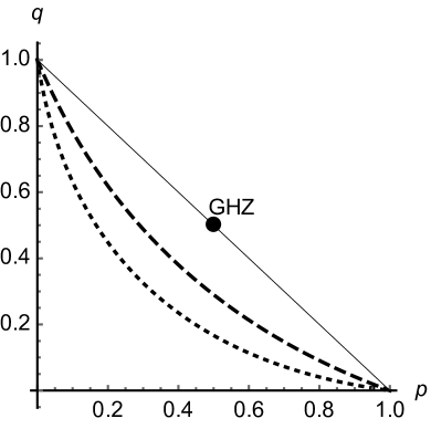
(a)

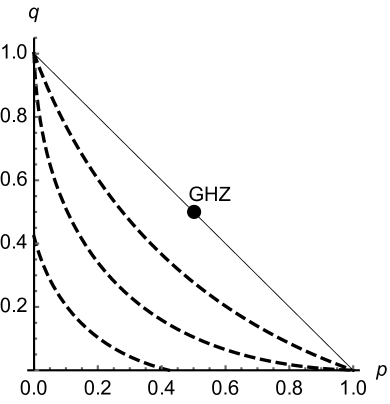
(b)

Figure 2: (a) For the triangle network we compare the criterion in Eq. (9) (dotted line) to the monogamy criterion in Eq. (14) (dashed line). (b) Results of the GHZ-type distribution in Eq. (7) using Eq. (11) for $N=5$ and $k=4,3,2$. Everything above the lines is detected to be incompatible with the respective network structure. $GHZ$ denotes the distribution that is obtained from measuring $\sigma_{z}$ on $\ket{GHZ}$.

Networks with dichotomic measurements.— For dichotomic measurements, that is, measurements with two outcomes, one can expect from our discussion after Eq. (2) that the covariance matrix can be simplified. Indeed, with our feature map the blocks of the covariance matrix are always of the form $(\Gamma_{\alpha\beta})_{ij}=(p_{ij}-q_{i}r_{j})$, where $p_{ij}$ is a probability distribution, and $q_{i}=\sum_{j}p_{ij}$ and $r_{j}=\sum_{i}p_{ij}$ are its marginals. These blocks have vanishing row and column sums, so $(1,\dots,1)^{T}$ is a (left and right) eigenvector to the eigenvalue zero. For the dichotomic case, the blocks are $2\times 2$ matrices, so only one nonzero eigenvalue remains, and we must have $\Gamma_{\alpha\beta}\propto(\mathds{1}-\sigma_{x})$. So we have:

Observation 2.

Consider a network of $N$ vertices, where each node performs a dichotomic measurement. Then the covariance matrix $\Gamma(\mathbf{v})$ is of the form

$$\Gamma(\mathbf{v})=C\otimes(\mathds{1}-\sigma_{x}),$$ (5)

where $C$ is an $N\times N$ matrix.

So, for evaluating the criterion for $k$-completeness in the case of dichotomic measurements, one just has to check the $k$-level coherence of the matrix $C$. While this is, in general, still hard, the solution can directly be written down for the simplest non-trivial case of $k=2$ Ringbauer et al. (2018). Namely, it is known that a matrix $X$ has coherence number less than or equal to two if and only if the so-called comparison matrix $M(X)$ defined by

$$(M[X])_{ij}=\left\{\begin{array}[]{ll}\left|X_{ii}\right|&\text{ if }i=j\\ -\left|X_{ij}\right|&\text{ if }i\neq j\end{array}\right.$$ (6)

is positive semidefinite. Thus, we have:

Observation 3.

If the comparison matrix $M(C)$ coming from the covariance matrix has a negative eigenvalue, then the observed probability distribution is incompatible with a network of bipartite sources.

Example of a GHZ-type distribution.— Consider the family of distributions that have previously been studied in Refs. Renou et al. (2019b); Åberg et al. (2020)

$$P (x_{1},\dots,x_{N})=$$ (7)

$$p \delta_{0}^{(N)}+q\delta_{1}^{(N)}+(1-p-q)\frac{1-\delta_{0}^{(N)}-\delta_{1}^{(N)}}{2^{N}-2},$$

where $\delta_{i}^{(N)}=\prod_{j=1}^{N}\delta_{ix_{j}}$. For $p=q=\frac{1}{2}$ this corresponds to measuring locally $\sigma_{z}$ on an $N$-particle Greenberger-Horne-Zeilinger (GHZ) state $\ket{GHZ}=(\ket{00\dots 0}+\ket{11\dots 1})/\sqrt{2}$. The covariance matrix for this distribution reads

$$C=\Delta\mathds{1}+\chi\outerproduct{\mathbf{1}}{\mathbf{1}},$$ (8)

where $\Delta=2^{N-2}(1-p-q)/(2^{N}-2)$, $\chi=\tfrac{1}{4}[1-(p-q)^{2}]-\Delta$ and $|\mathbf{1}\rangle=\sum_{n=1}^{N}|n\rangle$. From Eq. (6) we can conclude that $C$ has coherence number less or equal two if and only if the matrix $M(C)=(\Delta+2\chi)\mathds{1}-\chi\outerproduct{\mathbf{1}}{\mathbf{1}}$ is positive semidefinite. This matrix has eigenvalues $\lambda_{1}=\Delta+2\chi$ and $\lambda_{2}=\Delta-(N-2)\chi$. It follows that $C$ is incompatible with a $2$-complete network if

$$q>p+\kappa-\sqrt{4\kappa p+(\kappa-1)^{2}},$$ (9)

where $\kappa=[(N-1)2^{N-2}]/[(N-2)(2^{N-1}-1)]$. This analytically recovers the numerical results from Ref. Åberg et al. (2020) and proves that the witness conjectured in this reference is indeed optimal for arbitrary $N$.

Multilevel coherence witnesses.— Due to the simple structure of the matrix $C$ in Eq. (8) we can completely characterize its multilevel coherence properties and so the underlying distributions according to their network topologies for arbitrary $N$. For this purpose we need the concept of coherence witnesses. Consider an arbitrary pure state $\ket{\psi}=\sum_{i=1}^{M}c_{i}\ket{i}$. A $(k+1)$-level coherence witness is given by Ringbauer et al. (2018)

$$W_{k}=\mathds{1}-\frac{1}{\sum_{i=1}^{k}|c_{i}^{\downarrow}|^{2}}\outerproduct{\psi}{\psi},$$ (10)

where $c_{i}^{\downarrow}$ denote the coefficients $c_{i}$ reordered decreasingly according to their absolute values. This means that $\tr[W_{k}\varrho]\geq 0$, if $\varrho$ has coherence number $k$ or less. For the maximally coherent state $\ket{\psi^{+}}=(\sum_{i=1}^{N}\ket{i})/{\sqrt{N}}$ this witness is of the form $W_{k}=\mathds{1}-\outerproduct{\mathbf{1}}{\mathbf{1}}/k$. This witness can easily be proven to be optimal for the family of states $\varrho(\mu)=\mu\outerproduct{\psi^{+}}{\psi^{+}}+(1-\mu)\frac{\mathds{1}}{N}$, which is, up to normalisation and suitable choice of the parameter $\mu$, equivalent to $C$. Thus we obtain $\tr[W_{k}C]=(1-1/k)\Delta+(1-N/k)\chi$. From this, it directly follows that $C$ is incompatible with a $k$-complete network, if

$$q>p+\eta-\sqrt{4\eta p+(\eta-1)^{2}},$$ (11)

with $\eta=(N-1)2^{N-2}/[(N-k)(2^{N-1}-1)]$. The results are shown for the case $N=5$ and $k=4,3,2$ in Fig. 2b. Furthermore, we note that this technique can be applied to large networks where an approach based on SDPs would become infeasible, due to the rapidly growing number of terms in Eqs. (3, 4), which grows as $N\choose k$.

Networks beyond dichotomic measurements.— In the case of more than two outcomes per measurement, the block coherence number of the covariance matrix needs to be tested. For the case of networks involving only bipartite sources we have the following:

Observation 4.

Let $\Gamma(\mathbf{v})\in\mathcal{BC}_{2}$ be a covariance matrix with block coherence number two. Then, whenever the signs of some off-diagonal blocks are flipped such that the matrix remains symmetric, the resulting matrix will also remain positive semidefinite.

To see this, note that any matrix with block coherence number two can be written as a convex combination of pure states with coherence rank two, i.e., $\ket{\psi}=P_{i}\ket{\psi}+P_{j}\ket{\psi}$. For any such state, adding a minus sign in the density operator corresponds to the transformation $P_{i}\ket{\psi}+P_{j}\ket{\psi}\mapsto P_{i}\ket{\psi}-P_{j}\ket{\psi}$, under which the density operator remains positive semidefinite.

To demonstrate the power of this Observation, let us consider again the GHZ-type distribution, but now with three outcomes per measurement,

$$P(x_{1},x_{2},x_{3})= p \delta_{0}^{(3)}+q\delta_{1}^{(3)}+r\delta_{2}^{(3)}$$

$$+ (1-p-q-r)\frac{1-\delta_{0}^{(3)}-\delta_{1}^{(3)}-\delta_{2}^{(3)}}{3^{3}-3}.$$

A straightforward calculation provides a regime where this is incompatible with the triangle network, see Fig. 3.

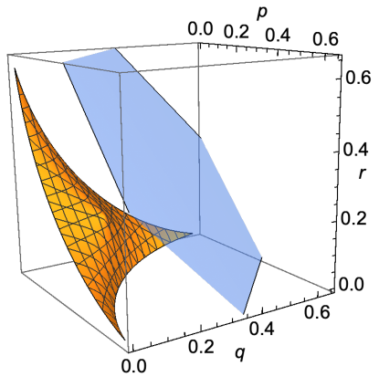
Figure 3: Analysis of the GHZ-type distribution with three outcomes per measurement in Eq. (Characterizing Quantum Networks: Insights from Coherence Theory) using Observation 4. Everything above the orange surface is detected to be incompatible with the triangle network. The blue surface represents the normalization constraint.

Characterizing networks with monogamy relations.— Another possibility to characterize networks is to evaluate monogamy relations for the coherence between different subspaces Kraft and Piani (2019). The idea is that the amount of coherence that can be shared between one subspace and all other subspaces is limited if a certain block coherence number is imposed. To be more precise, for a trace one positive semidefinite block matrix $X=\quantity[X_{\alpha\beta}]_{\alpha,\beta=0}^{N}$ with block coherence number $k$ it holds that

$$\sum_{\beta=1}^{N}\left\|X_{0\beta}\right\|_{\rm tr}\leq\sqrt{k-1}\sqrt{\tr[X_{00}](1-\tr[X_{00}])}.$$ (13)

If we consider the normalized matrix matrix $\tilde{C}=C/\tr[C]$, evaluating such a monogamy relation provides a necessary criterion for $C$ to have coherence number $k$. For the matrix in Eq. (8) this gives

$$\Delta-(\frac{\sqrt{N-1}}{\sqrt{k-1}}-1)\chi\geq 0.$$ (14)

Hence, if this inequality is violated then the observed correlations are not compatible with a $k$-complete network. This is also shown in Fig. 2a for the triangle network. Although this test is in this case not as powerful as the analytical solution, it is easy to evaluate especially for large networks, since it requires only computing traces of smaller block matrices.

Further remarks.— So far, we provided criteria to show that correlations are incompatible with a $k$-complete network. It would be interesting to derive also sufficient criteria for being compatible with a given network structure. In the framework of Ref. Åberg et al. (2020) this is not directly possible, as the criterion in Eqs. (3, 4) is a convex relaxation of the original problem. Still, coherence theory allows to identify scenarios where the covariance matrix can be certified to have a small block coherence number $k$, so the covariance matrix approach must fail to prove incompatibility with a $k$-complete network.

Here we can make two small observations in this direction: (i) The following results from Ref. Ringbauer et al. (2018) can directly applied to networks with dichotomic outcomes. Namely, if we have for the normalized matrix $\tilde{C}\geq\frac{N-k}{N-1}\Lambda(\tilde{C})$, where $\Lambda$ is the fully decohering map, mapping any matrix to its diagonal part, then $\tilde{C}\in\mathcal{BC}_{k}$, implying that the test in Eqs. (3, 4) for $(k+1)$-complete networks will fail. Furthermore we have that if $\tr[\tilde{C}^{2}]/\tr[\tilde{C}]^{2}\leq 1/(N-1)$, then $\tilde{C}$ is two-level coherent. (ii) In the general case, if $M_{b}(\Gamma)\geq 0$, where $M_{b}(\Gamma)$ is the block comparison matrix defined by

$$(M_{b}[\Gamma])_{\alpha\beta}=\begin{cases}(\norm*{\Gamma_{\alpha\alpha}^{-1}})^{-1}&\text{for $\alpha=\beta$}\\ -\norm{\Gamma_{\alpha\beta}}&\text{for $\alpha\neq\beta$,}\end{cases}$$ (15)

with $\norm{X}$ denoting the largest singular value of the block $X$, then $\Gamma\in\mathcal{BC}_{2}$. A detailed discussion is given in the Appendix.

Conclusion.— In this work we have established a connection between the theory of multilevel coherence and the characterization of quantum networks. To be precise, we showed that a recent approach based on covariance matrices leads to a well studied problem in coherence theory; consequently, many results from the latter field can be transfered to the former. This provides a useful application of the resource theory of multilevel coherence outside of the usual realm of quantum states.

There are several interesting problems remaining for future work. First, it would be highly desirable to extend the covariance approach to the case where each node of the network can perform more than one measurement. This will probably lead to significantly refined tests for network topologies. Second, it seems to be promising to study the coherence in networks on the level of the resulting quantum state, and not the covariance matrix. This may shed light on the question which types of network correlations are useful for applications in quantum information processing.

Appendix A Appendix: Sufficient conditions for block coherence number two

Let the block matrix $X=\quantity[X_{\alpha\beta}]>0$, with $X_{\alpha\beta}\in\mathds{C}^{d\times d}$, be partitioned as follows

$$X=\left[\begin{array}[]{cccc}X_{11}&X_{12}&\cdots&X_{1K}\\ X_{21}&X_{22}&\cdots&X_{2K}\\ \vdots&\vdots&\ddots&\vdots\\ X_{K1}&X_{K2}&\cdots&X_{KK}\end{array}\right].$$ (16)

Definition 5 (from Ref. Feingold and Varga (1962)).

Let $X$ be partitioned as in Eq. (16). If the matrices $X_{\alpha\alpha}$ on the diagonal are non-singular, and if

$$(\norm*{X_{\alpha\alpha}^{-1}})^{-1}\geq\sum_{\begin{subarray}{c}\beta=1\\ \beta\neq\alpha\end{subarray}}^{K}\norm{X_{\alpha\beta}},$$ (17)

then $X$ is called block diagonally dominant. Here, $\norm{Y}$ denotes the largest singular value, so for the positive $X_{\alpha\alpha}$ the expression $\norm{X_{\alpha\alpha}^{-1}}^{-1}$ is the smallest eigenvalue of $X_{\alpha\alpha}$.

Observation 6.

If $X$ is positive and block diagonally dominant, then the block coherence number is smaller or equal to two, $bcn(X)\leq 2$.

Proof.

Suppose $X$ satisfies the hypothesis. Define $2\times 2$ block matrices

$$G^{\alpha\beta}=\matrixquantity[\absolutevalue{X_{\alpha\beta}}&&X_{\alpha\beta}\\ X_{\alpha\beta}^{\dagger}&&\absolutevalue{X_{\alpha\beta}^{\dagger}}],$$ (18)

where $\absolutevalue{X_{\alpha\beta}}=\sqrt{X_{\alpha\beta}^{\dagger}X_{\alpha\beta}}$ and the support of $G^{\alpha\beta}$ is the subspace $\alpha,\beta$. Clearly, the $G^{\alpha\beta}$ are positive semidefinite and have block coherence number two. Next, consider the matrix $D=X-\sum_{\alpha=1}^{K}\sum_{\beta>\alpha}G^{\alpha\beta}$. Since $X>0$ it is also hermitian, and thus, $X_{\beta\alpha}=X_{\alpha\beta}^{\dagger}$, precisely as for $G^{\alpha\beta}$. From this we can conclude that the off-diagonal blocks of $D$ vanish and the diagonal blocks are given by $D_{\alpha\alpha}=X_{\alpha\alpha}-\sum_{\begin{subarray}{c}\beta=1,\beta\neq\alpha\end{subarray}}^{K}\absolutevalue{X_{\alpha\beta}}$. Furthermore, observe that $\lambda_{\text{min}}(X_{\alpha\alpha})\geq\sum_{\begin{subarray}{c}\beta=1,\beta\neq\alpha\end{subarray}}^{K}\lambda_{\text{max}}(X_{\alpha\beta})\geq\lambda_{\text{max}}(\sum_{\begin{subarray}{c}\beta=1,\beta\neq\alpha\end{subarray}}^{K}X_{\alpha\beta})$, where the first inequality is due to Eq. (17) and the second inequality is straightforward. This proves that, besides being block diagonal, $D$ is also positive semidefinite. Thus $X$ can be written as a positive sum of a block incoherent matrix $D$ and matrices $G^{\alpha\beta}$ of block coherence number two, from which the statement follows. ∎

The next concept that is needed is the so-called comparison matrix, which is defined as follows.

Definition 7 (from Ref. Polman (1987)).

Let $X$ be partitioned as in Eq. (16) and $X_{\alpha\alpha}$ non-singular. Then the block comparison matrix $M_{b}[X]$ is defined by

$$(M_{b}[X])_{\alpha\beta}=\begin{cases}(\norm*{X_{\alpha\alpha}^{-1}})^{-1}&\text{for $\alpha=\beta$}\\ -\norm{X_{\alpha\beta}}&\text{for $\alpha\neq\beta$.}\end{cases}$$ (19)

From this definition it is evident that if the comparison matrix $M_{b}[X]$ exists and is (strictly) diagonally dominant, then $X$ itself is (strictly) block diagonally dominant.

Definition 8 (M-matrix).

Let the matrix $A=(a_{ij})$ be a real matrix such that $a_{ij}\leq 0$ for $i\neq j$. Then $A$ is called a nonsingular M-matrix if and only if every real eigenvalue of $A$ is positive.

Definition 9 (Def. 3.2. in Ref. Polman (1987)).

If there exist nonsingular block diagonal matrices $D$ and $E$ such that $M_{b}[DXE]$ is a nonsingular M-matrix, then $X$ is said to be a nonsingular block H-matrix.

Lemma 10 (Lemma 4. in Ref. Polman (1987)).

If $X$ is a nonsingular block H-matrix then there exist nonsingular block diagonal matrices $D$ and $E$ such that $DXE$ is strictly block diagonally dominant.

Theorem 11.

Let $X$ be partitioned as in Eq. (16) and positive semidefinite (but not necessarily strictly positive). If $M_{b}(X)\geq 0$, then $X$ has $bcn(X)\leq 2$.

Proof.

The proof follows the idea of Ref. Ringbauer et al. (2018). First, define the operator $X_{\epsilon}=X+\epsilon\mathds{1}$, for $\epsilon\geq 0$. Then, for $\epsilon>0$ we have that $M_{b}[X_{\epsilon}]=M[X]+\epsilon\mathds{1}>0$. Evidently, since $M_{b}[X_{\epsilon}]$ is a real matrix with non-positive off-diagonal entries and furthermore has only strictly positive eigenvalues it is a nonsingular M-matrix, according to Def. 8. Then, according to Def. 9 $X_{\epsilon}$ is a nonsingular block H-matrix. From the proof of Lemma 10 in Ref. Polman (1987) we can conclude that there exists a block diagonal matrix $D>0$ such that $D_{\epsilon}X_{\epsilon}D_{\epsilon}$ is strictly block diagonally dominant. Then it follows from Observation 6 that strictly block diagonally dominant matrices can have at most block coherence number two. We find that $bcn(X_{\epsilon})=bcn(D_{\epsilon}X_{\epsilon}D_{\epsilon})\leq 2$, and since the block coherence number is lower semi-continuous we have $bcn(X)=bcn(\lim_{\epsilon\rightarrow 0^{+}}X_{\epsilon})\leq\lim_{\epsilon\rightarrow 0^{+}}bcn(X_{\epsilon})\leq 2$. ∎

References

- Kimble (2008) H. J. Kimble, Nature 453, 1023 (2008).
- Sangouard et al. (2011) N. Sangouard, C. Simon, H. de Riedmatten, and N. Gisin, Rev. Mod. Phys. 83, 33 (2011).
- Simon (2017) C. Simon, Nat. Phot. 11, 678 (2017).
- Wehner et al. (2018) S. Wehner, D. Elkouss, and R. Hanson, Science 362 (2018).
- Cirac et al. (1998) J. I. Cirac, S. J. van Enk, P. Zoller, H. J. Kimble, and H. Mabuchi, Physica Scripta T76, 223 (1998).
- Gisin et al. (2002) N. Gisin, G. Ribordy, W. Tittel, and H. Zbinden, Rev. Mod. Phys. 74, 145 (2002).
- Spirtes et al. (2000) P. Spirtes, C. Glymour, and R. Scheines, Causation, Prediction, and Search (MIT press, 2000).
- Pearl (2009) J. Pearl, Causality (Cambridge University Press, 2009).
- Renou et al. (2019a) M.-O. Renou, E. Bäumer, S. Boreiri, N. Brunner, N. Gisin, and S. Beigi, Phys. Rev. Lett. 123, 140401 (2019a).
- Gisin et al. (2020) N. Gisin, J.-D. Bancal, Y. Cai, P. Remy, A. Tavakoli, E. Zambrini Cruzeiro, S. Popescu, and N. Brunner, Nat. Commun. 11, 2378 (2020).
- Navascues et al. (2020) M. Navascues, E. Wolfe, D. Rosset, and A. Pozas-Kerstjens, (2020), arXiv:2002.02773 [quant-ph] .
- Kraft et al. (2020) T. Kraft, S. Designolle, C. Ritz, N. Brunner, O. Gühne, and M. Huber, (2020), arXiv:2002.03970 [quant-ph] .
- Luo (2020) M.-X. Luo, (2020), arXiv:2003.07153 [quant-ph] .
- Acín et al. (2001) A. Acín, D. Bruß, M. Lewenstein, and A. Sanpera, Phys. Rev. Lett. 87, 040401 (2001).
- Gühne and Tóth (2009) O. Gühne and G. Tóth, Phys. Rep. 474, 1–75 (2009).
- Kela et al. (2020) A. Kela, K. Von Prillwitz, J. Åberg, R. Chaves, and D. Gross, IEEE Trans. Inf. Theory 66, 339 (2020).
- Åberg et al. (2020) J. Åberg, R. Nery, C. Duarte, and R. Chaves, (2020), arXiv:2002.05801 [quant-ph] .
- Aberg (2006) J. Aberg, (2006), arXiv:quant-ph/0612146 [quant-ph] .
- Baumgratz et al. (2014) T. Baumgratz, M. Cramer, and M. B. Plenio, Phys. Rev. Lett. 113, 140401 (2014).
- Killoran et al. (2016) N. Killoran, F. E. S. Steinhoff, and M. B. Plenio, Phys. Rev. Lett. 116, 080402 (2016).
- Regula et al. (2018) B. Regula, M. Piani, M. Cianciaruso, T. R. Bromley, A. Streltsov, and G. Adesso, New J. Phys. 20, 033012 (2018).
- Streltsov et al. (2017a) A. Streltsov, G. Adesso, and M. B. Plenio, Rev. Mod. Phys. 89, 041003 (2017a).
- Chitambar and Gour (2019) E. Chitambar and G. Gour, Rev. Mod. Phys. 91, 025001 (2019).
- Winter and Yang (2016) A. Winter and D. Yang, Phys. Rev. Lett. 116, 120404 (2016).
- Chitambar and Hsieh (2016) E. Chitambar and M.-H. Hsieh, Phys. Rev. Lett. 117, 020402 (2016).
- Streltsov et al. (2017b) A. Streltsov, S. Rana, M. N. Bera, and M. Lewenstein, Phys. Rev. X 7, 011024 (2017b).
- Ringbauer et al. (2018) M. Ringbauer, T. R. Bromley, M. Cianciaruso, L. Lami, W. Y. S. Lau, G. Adesso, A. G. White, A. Fedrizzi, and M. Piani, Phys. Rev. X 8, 041007 (2018).
- Kraft and Piani (2019) T. Kraft and M. Piani, (2019), arXiv:1911.10026 [quant-ph] .
- Boyd and Vandenberghe (2004) S. Boyd and L. Vandenberghe, Convex Optimization (Cambridge University Press, Cambridge, 2004).
- Gärtner and Matoušek (2012) B. Gärtner and J. Matoušek, Approximation Algorithms and Semidefinite Programming (Springer Verlag, Berlin, Heidelberg, 2012).
- Johnston et al. (2018) N. Johnston, C.-K. Li, S. Plosker, Y.-T. Poon, and B. Regula, Phys. Rev. A 98, 022328 (2018).
- Renou et al. (2019b) M.-O. Renou, Y. Wang, S. Boreiri, S. Beigi, N. Gisin, and N. Brunner, Phys. Rev. Lett. 123, 070403 (2019b).
- Feingold and Varga (1962) D. G. Feingold and R. S. Varga, Pacific J. Math. 12, 1241 (1962).
- Polman (1987) B. Polman, Linear Algebra Its Appl. 90, 119 (1987).