SPISEA: A Python-Based Simple Stellar Population Synthesis Code for Star Clusters

Abstract

We present SPISEA (Stellar Population Interface for Stellar Evolution and Atmospheres), an open-source Python package that simulates simple stellar populations. The strength of SPISEA is its modular interface which offers the user control of 13 input properties including (but not limited to) the Initial Mass Function, stellar multiplicity, extinction law, and the metallicity-dependent stellar evolution and atmosphere model grids used. The user also has control over the Initial-Final Mass Relation in order to produce compact stellar remnants (black holes, neutron stars, and white dwarfs). We demonstrate several outputs produced by the code, including color-magnitude diagrams, HR-diagrams, luminosity functions, and mass functions. SPISEA is object-oriented and extensible, and we welcome contributions from the community. The code and documentation are available on GitHub and ReadtheDocs, respectively.

1 Introduction

The ability to simulate stellar populations is an essential tool for interpreting observations of star clusters. Many star clusters can be modeled as simple stellar populations (SSPs), which are characterized by a single age and metallicity. The need for fast SSP generation has become increasingly important as the importance of stochasticity in interpreting observed populations has been more widely recognized (e.g. Cerviño, 2013; Krumholz et al., 2015). Furthermore, forward modeling analysis techniques require codes that can quickly produce SSPs within likelihood functions (e.g. Lu et al., 2013; Hosek et al., 2019b).

A range of codes that simulate stellar populations are available in the literature, each offering different advantages. Examples such as Starburst99 (Leitherer et al., 1999; Vázquez & Leitherer, 2005), PEGASE (Fioc & Rocca-Volmerange, 1997, 2019), GALAXEV (Bruzual & Charlot, 2003), GALICS (Hatton et al., 2003), the evolutionary population synthesis models from Maraston (1998, 2005); Maraston et al. (2020), PopStar (Mollá et al., 2009), Flexible Stellar Population Synthesis (FSPS; Conroy et al., 2009; Conroy & Gunn, 2010), CIGALE (Noll et al., 2009) and Stochastically Lighting Up Galaxies (SLUG; da Silva et al., 2012; Krumholz et al., 2015) can be used to model SSPs and composite stellar populations (i.e., those with multiple ages and/or metallicities). These codes are commonly used to model unresolved galaxy populations, typically offering features such as models for dust attenuation, calculation of the photoionization and resulting nebular emission from the interstellar medium, and prescriptions for the chemical yields of supernovae and the resulting chemical evolution of the region. Other codes such as Binary Population and Spectral Synthesis (BPASS; Eldridge et al., 2017; Stanway & Eldridge, 2018) and SYCLIST (Georgy et al., 2014) specialize in SSPs, offering advanced treatment of binary stellar evolution and stellar rotation, respectively. BPASS also offers nebular emission calculations for HII regions with their model populations (Xiao et al., 2018) as well as a convenient Python interface (Hoki; Stevance et al., 2020).

However, a limitation of these codes is that they often force the user to choose between a fixed set of options when choosing the “ingredients” to construct the stellar populations, such as the initial mass function (IMF), extinction law, stellar multiplicity properties, and/or the initial-final mass relation (IFMR). This can be a necessary restriction due to the complexity of the underlying calculations (e.g., calculating nebular emission via radiative transfer or modeling binary stellar evolution), but it hinders the ability to forward model these properties in observed populations.

To address this, we present SPISEA (Stellar Population Interface for Stellar Evolution and Atmospheres), an open-source Python package that generates resolved and unresolved SSPs. SPISEA serves as a modular interface to existing stellar evolution and stellar atmosphere grids, allowing the user to create star clusters with control over a range of input parameters. These span from basic properties represented by a single input value (age, metallicity, distance, extinction, differential extinction and initial cluster mass) to more complex properties which are represented as code objects (IMF, extinction law, multiplicity properties, photometric filters, and IFMR). The stellar evolution and atmosphere grids are also presented as code objects that the user can select from. This structure provides significant flexibility as the code objects are straight forward to manipulate, and the user can create new sub-classes in order to implement new models and/or functionalities that be integrated with the rest of the code.

The usefulness of SPISEA has been demonstrated in several published studies: modeling the IMF of star clusters (Lu et al., 2013; Hosek et al., 2019b), measuring the extinction law in highly reddened regions (Hosek et al., 2018), predicting black hole microlensing rates (Lam et al., 2020), and calculating photometric transformations at high extinction and with a non-standard extinction law (Krishna Gautam et al., 2019; Chen et al., 2019). SPISEA can be downloaded via GitHub with documentation provided through ReadtheDocs. A permanent Digital Object Identifier (DOI) has been created to document this release of the code.

A top-level overview of the code is presented in $\mathsection$2. A description of how cluster isochrones and populations are generated is provided in $\mathsection$3 and $\mathsection$4, respectively, and code examples are shown in $\mathsection$5. In $\mathsection$6 we discuss the current limitations of SPISEA along with future directions for development, in $\mathsection$7 we discuss how to contribute to the code, and then in $\mathsection$8 we present our conclusions.

2 SPISEA Overview

SPISEA has the following capabilities:

• Build a theoretical cluster isochrone at a given age, distance, extinction, and metallicity. Each star is assigned intrinsic properties using metallicity-dependent stellar evolution and atmosphere grids. Synthetic photometry is calculated for a set of photometric filters defined by the user, if desired ($\mathsection$3).

• Simulate a star cluster given an isochrone at the chosen age and metallicity, initial mass, IMF, and multiplicity. Differential extinction can be added if desired. The output can either be resolved, which produces tables of physical properties and synthetic photometry for the individual star systems, or unresolved, which produces the composite spectrum of the stellar population ($\mathsection$4).

• Calculate the population of compact stellar remnants produced by a cluster at any age using an IFMR. The type and mass of each compact object is returned ($\mathsection$4.3).

A top-level diagram of the workflow of the code is shown in Figure 1. Tables with the pre-loaded set of stellar evolution and atmosphere models, extinction laws, and photometric filters are provided in Appendix A.

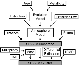
Figure 1: Diagram of the SPISEA code. The open boxes represent inputs specified by the user. The primary outputs are the Isochrone ($\mathsection$3.5) and Cluster ($\mathsection$4.5) objects, which are represented by shaded boxes.

3 Building a Theoretical Cluster Isochrone

SPISEA builds a theoretical cluster isochrone using existing stellar evolution and stellar atmosphere model grids. The stellar evolution model provides basic stellar properties (e.g. current stellar mass, effective temperature T_eff, surface gravity log $g$, and luminosity $L$) at a given age as a function of initial stellar mass. The stellar atmosphere model then uses this information to assign a spectrum to each stellar mass. The primary inputs provided by the user are the isochrone age, distance, extinction, and metallicity, as well as what evolution and atmosphere model grids to use. Table 3 describes the range of ages and metallicities available for the different evolution model grids in addition to the range of T_eff, log $g$, and metallicies available for the different atmosphere model grids.

3.1 Stellar Evolution Models

Stellar evolution models are defined as sub-classes off the main evolution.StellarEvolution object. The user selects which model grid to use by selecting the appropriate sub-class. Several popular evolution model grids such as MIST (Choi et al., 2016), Geneva (Ekström et al., 2012), and Parsec (Bressan et al., 2012) come pre-packaged with SPISEA and already have sub-classes defined (Appendix A). In addition, there are several hybrid grids that combine models across different regions of parameter space to take advantage of their individual strengths (e.g. old vs. young populations, pre-main sequence vs. main sequence stars, etc.). These hybrid grids are discussed in Appendix B. The user can also implement a new evolution model grid by defining their own evolution.StellarEvolution sub-class and pointing it to a directory containing the grid of isochrones produced by that model.

3.2 Stellar Atmosphere Models

Stellar atmosphere model grids are accessed via the get_atmosphere functions defined in atmospheres.py. Each atmosphere model has its own get_atmosphere function, with grids such as ATLAS9 (Castelli & Kurucz, 2004), PHOENIX (Husser et al., 2013), and BTSettl (Allard et al., 2012b, a; Baraffe et al., 2015) already defined (Appendix A). Similar to the evolution models, a hybrid atmosphere model function has been defined which uses different atmosphere grids depending on the effective temperature range requested (Appendix B). In addition, the user can define their own get_atmosphere functions to create a mix of the provided model atmosphere grids or implement a new grid entirely.

Stellar spectra are assigned from the atmosphere grid to each star in the evolution model using Space Telescope Science Institute’s pysynphot framework (STScI Development Team, 2013). For each star, pysynphot searches the grid to find the best-matching atmosphere in T_eff, log $g$, and metallicity ([Z]), interpolating between models where necessary. The spectra are originally in surface flux units (ergs cm^-2 s^-1 Å^-1), and are multiplied by a factor of (R / D)², where R is the stellar radius (taken from the evolution model) and D is the given distance (specified by the user) to produce the unreddened flux of the star at Earth.

The stellar atmosphere models have default wavelength range of 0.3 $\mu$m – 5.2 $\mu$m, though the user can extend this to up to 0.1 $\mu$m – 10 $\mu$m if desired. However, before extending the wavelength range, the user should confirm that their chosen atmosphere models cover the desired range (see Table 3). By default, the spectral resolution of the atmospheres have been reduced to match the ATLAS9 grid (Castelli & Kurucz, 2004), which corresponds to R $\sim$ 250. This is generally sufficient for the purposes of synthetic photometry. Versions of the atmosphere models at their original resolution (also in Table 3) are available for download with SPISEA, but calculating synthetic photometry at these high resolutions is significantly slower.

3.3 Extinction

Extinction is applied to the synthetic stellar spectra using the total extinction and an extinction law. The total extinction is parameterized as A_K, the total magnitudes of extinction at K-band, and the extinction law is defined as A_λ / A_K. The total extinction at a given wavelength is thus:

$$A_{\lambda}=A_{K}*(A_{\lambda}/A_{K})$$ (1)

and the reddened flux F_r at $\lambda$ is:

$$F_{r}(\lambda)=F_{i}*10^{-0.4*A_{\lambda}}$$ (2)

where F_i is the unreddened flux of the star.

SPISEA again uses the pysynphot framework for this calculation, and the extinction law is defined as sub-class of the pysynphot.reddening.CustomRedLaw object. The set of pre-defined extinction laws include those from Cardelli et al. (1989), Nishiyama et al. (2009), and Schlafly et al. (2016). The user can also define a power-law extinction law with an arbitrary exponent using the RedLawPowerLaw sub-class.

3.4 Synthetic Photometry

The user can calculate synthetic photometry for the stars in the isochrone object. Filter transmission functions are defined as pysynphot.ArrayBandpass objects, which are convolved with the source spectrum to calculate the flux in a given filter. In this first release of SPISEA, the source spectra are defined between 0.25 $\mu$m – 5.2 $\mu$m.

Stellar magnitudes are calculated in the Vega system:

$$m_{s}=-2.5*log(F_{s}/F_{Vega})+M_{Vega}$$ (3)

where $F_{s}$ is the integrated flux of the source star in the filter, $F_{Vega}$ are the integrated flux of the Vega star model in the filter, and $M_{Vega}$ = 0.03 mag is the magnitude of Vega in the filter. We adopt a Kurucz atmosphere with T_eff = 9550 K, log $g$ = 3.95, and [Z] = -0.5 as a model for Vega (Castelli & Kurucz, 1994), and assume $(R/d)^{2}$ = 6.247x10^-17, where $R$ is the stellar radius and $d$ is the distance of Vega (Girardi et al., 2002).

Additional photometric calibrations (such as AB magnitudes) are not yet supported by SPISEA. If this functionality is desired, the user can request it via the Github issues page ($\mathsection$7).

3.5 Isochrone Output

A SPISEA isochrone is defined as a synthetic.Isochrone object. If synthetic photometry is desired, then the synthetic.IsochronePhot sub-class should be used. All synthetic.Isochrone objects contain an array with the reddened spectra for each star, while the synthetic.IsochronePhot sub-class contains an additional Astropy table (Astropy Collaboration et al., 2013, 2018) with the stellar parameters and synthetic photometry in a specified set of filters. A description of the columns in the output table is provided in Table 1.

The table from synthetic.IsochronePhot is saved in FITS table format with a standard file name in a directory specified by the user. When synthetic.IsochronePhot is called, it will first search the specified directory to see if the file already exists. If it does, it will simply read the file rather than redoing the full isochrone calculation. Thus, generating a grid of synthetic.IsochronePhot isochrones can save considerable time when analyzing an observed stellar population.

Table 1: Isochrone Table Output

Column	Description	Units
L	Luminosity	W
Teff	Effective Temperature	K
R	Radius	m
mass	Initial Mass	M⊙
logg	Surface Gravity	cgs
isWR	Is star a Wolf-Rayet?	boolean
mass_current	Current Mass	M⊙
phase	Evolution Phase
m_*	Magnitude in filters	Vega Mag

4 Making A cluster

Once an isochrone has been created, the user can create a synthetic cluster by specifying the stellar multiplicity, IMF, IFMR, differential extinction, and initial cluster mass. Various aspects of generating a synthetic cluster have been described in sections of Lu et al. (2013), Hosek et al. (2019b), and Lam et al. (2020), but we collate and summarize the process here.

4.1 Multiplicity

Surveys of nearby stellar populations reveal that the fraction of multiple systems is high, rising from roughly 20% for M $\sim$ 0.1 M_⊙ stars to nearly 100% for M $\gtrsim$ 5 M_⊙ stars (e.g. Sana et al., 2012; Duchêne & Kraus, 2013). Further, the properties of these systems have been shown to vary as a function of primary mass (Moe & Di Stefano, 2017). In SPISEA, one can construct a Multiplicity object (multiplicity.MultiplicityUnresolved) that defines the multiplicity fraction ($MF$), companion star frequency ($CSF$), and mass ratio ($q$) of synthetic cluster.

Following Reipurth & Zinnecker (1993), the $MF$ describes the fraction of stars that host multiple systems:

$$MF=\frac{B+T+Q+...}{S+B+T+Q+...}$$ (4)

where $S$ is the number of single stars, $B$ is the number of binary stars, $T$ is the number of triple stars, $Q$ is the number of quadruple systems, and so forth. The $CSF$ describes the expected number of companions in a given multiple system:

$$CSF=\frac{B+2T+3Q+...}{S+B+T+Q+...}.$$ (5)

Finally, the mass ratio $q$ defines the ratio between the primary star mass and the companion star mass.

For each star drawn from the IMF ($\mathsection$ 4.2), its multiplicity properties are drawn from the $MF$, $CSF$, and $q$ distributions and companion stars assigned accordingly. All multiple systems are assumed to be unresolved, and the individuals fluxes of the stars are added together to produce the final synthetic photometry of the system. Note that SPISEA does not yet include the orbital properties of the multiple systems, such as binary separation or eccentricity. In addition, the impact of multiplicity on stellar evolution is also ignored. The implementation of orbital properties and binary stellar evolution models is left for future versions of SPISEA ($\mathsection$6).

The default parameters for
multiplicity.MultiplicityUnresolved are defined in Lu et al. (2013), who define empirical functions for $MF$, $CSF$, and $q$ based on observations of young clusters ($<$10 Myr). The $MF$ and $CSF$ are defined as power laws as a function of the stellar mass:

$$MF(m)=A*m^{\alpha}$$ (6)

$$CSF(m)=B*m^{\beta}$$ (7)

where $A$ = 0.44, $\alpha$ = 0.51, $B$ = 0.50, $\beta$ = 0.45, and $m$ is the stellar mass in units of solar masses. The $MF$ is defined over a range from [0,1] and the $CSF$ is defined from [0, 3]. If a given stellar mass is large enough that the $MF$ of $CSF$ would be larger than their maximum values, they are simply set to the maximum value itself.

Finally, the probability distribution for $q$ is defined as a single power law with no mass dependence:

$$P(q)=\left(\frac{1+\gamma}{1-q_{lo}^{1+\gamma}}\right)*q^{\gamma}$$ (8)

where $\gamma$ = -0.4 and $q_{lo}$, which represents the lowest allowed mass ratio, is 0.01.

The user can change the values for $A$, $B$, $\alpha$, $\beta$, $\gamma$, max $CSF$, and $q_{lo}$ in multiplicity.MultiplicityUnresolved by adjusting the appropriate keyword arguments.

4.2 Initial Mass Function

The IMF describes the initial distribution of stellar masses in a star cluster. While the true functional form(s) of the IMF is unknown, it is often described a log-normal or broken power-law distribution (e.g. Bastian et al., 2010). SPISEA defines the IMF as an imf.IMF object, and currently supports a broken power-law functional form as defined by the sub-class imf.IMF_broken_powerlaw. The user has control over the number of power-law segments, the power-law slope for each segment, the break masses between segments, and stellar mass range the IMF is defined over. The Multiplicity object is an additional input for the IMF object that describes the multiplicity properties of the population ($\mathsection$ 4.1).

Several standard broken power-law IMFs are included such as from Salpeter (1955), Miller & Scalo (1979), Kroupa (2001), and Weidner & Kroupa (2004). Functional forms other than broken power-laws may be added as additional sub-classes of the imf.IMF object, but this is beyond the scope of the initial code release ($\mathsection$6).

SPISEA uses the algorithm described by Pflamm-Altenburg & Kroupa (2006) to stochastically draw stars from the IMF until the initial cluster mass is reached. First, a rough estimate of the total number of stars in the cluster is made (the initial cluster mass divided by the average stellar mass in the IMF). Then stars are drawn from the IMF in batches equal to 10% of the total number of stars and are assigned companions according to the input multiplicity model. This continues until the cumulative mass of all stars (including companions) is closest to the initial cluster mass. This process is most similar to the STOP_NEAREST stochastic sampling technique defined in SLUG (Krumholz et al., 2015).

Note that no age information is used at this point and all sampling is done on the initial stellar mass and the initial cluster mass, not the present-day masses. Once these initial masses are drawn, we use the stellar evolution model for the input population age and metallicity to determine the current properties of the stars, as discussed in section $\mathsection$3.1.

4.3 Initial-Final Mass Relation

The IFMR maps a star’s initial mass, also called the zero-age main sequence (ZAMS) mass, to the type and mass of the compact object it will form (e.g. Portinari et al., 1998; Kalirai et al., 2008; Sukhbold et al., 2016; Raithel et al., 2018). It is an active area of study, in particular at high stellar masses where the IFMR is not well constrained. In SPISEA, the user can define an IFMR object (ifmr.IFMR) to simulate the compact objects produced by a stellar population.

The default SPISEA IFMR object is a combination of two IFMRs in the literature: one for white dwarfs (WD), and another for neutron stars (NS) and black holes (BH). The WD IFMR comes from Kalirai et al. (2008), and is derived from observations of open clusters. The NS/BH IFMR comes from Raithel et al. (2018), which is derived from the 1-D neutrino-driven supernova simulations of Sukhbold et al. (2016) coupled with the distribution of observed NS and BH masses. For a mathematical description of the default IFMR, see Lam et al. (2020).

The WD IFMR from Kalirai et al. (2008) is relatively straightforward, as the final WD mass only depends on the ZAMS mass. The NS/BH IFMR is more complicated as stellar metallicity, rotation, and core structure of the pre-supernova star have been found to play important roles in determining the type and mass of remnant formed (Heger et al., 2003; Sukhbold et al., 2018). As a result, Raithel et al. (2018) derive a probabilistic IFMR, where each ZAMS mass is assigned a probability of being a NS or BH. In SPISEA, each star of sufficient ZAMS mass are designated as NS or BH according to these probabilities. It should be noted that the IFMR of Raithel et al. (2018) is for single and solar metallicity stars. However, there are models with different metallicities and a binary IFMR that will be published in the near future (T. Sukhbold, private communication) that will be implemented in future versions of SPISEA. In addition, the user may define their own IFMR objects as they see fit.

All compact objects produced from the IFMR are assumed to be dark (e.g. zero luminosity) since we do not have the necessary evolution or atmosphere models to describe them. Although real WDs, NSs, and accreting BHs have non-zero luminosities, these objects are typically much fainter at optical/near-infrared wavelengths than the majority of the of the surrounding stellar population (e.g. Kalirai et al., 2008). Thus, this assumption has negligible impact on the cluster population photometry in most cases. However, improved treatment of these sources is an avenue of future code development.

The exception to this is the MISTv1 evolution models, which produce model parameters for a subset of the WD population. These models include stars down to the white dwarf cooling phase until $\Gamma=20$, where $\Gamma$ is the Coulomb coupling parameter (Choi et al., 2016). For these objects, a WD model atmosphere can be assigned (e.g. Koester, 2010) and synthetic photometry computed. However, objects with $\Gamma>20$, which are extremely cooled or crystallized, are not included in the MISTv1 models. In SPISEA, these objects will will be picked up by the Kalirai et al. (2008) IFMR to produce the aforementioned dark WDs.

4.4 Differential Extinction

Differential extinction is a phenomenon by which the stars within a cluster exhibit a distribution of extinction values rather than a constant value. This could occur due to variations in the density of foreground gas and dust along the line-of-sight to a cluster, and has been observed observed in several Milky Way clusters (e.g. Burki, 1975; Schödel et al., 2010; Habibi et al., 2013; Hosek et al., 2015; Andersen et al., 2017; Rui et al., 2019). The user can control the differential extinction through the $\sigma_{A_{K}}$ parameter. For each star, SPISEA will perturb the total extinction A_K (the magnitudes of extinction in K-band) by an amount $\delta A_{K}$ drawn from a Gaussian distribution with mean $\mu$ = 0 and standard deviation $\sigma$ = $\sigma_{A_{K}}$.

To derive the reddening vector of each photometric filter, the Vega model atmosphere is extinguished at both A_K and A_K + $\sigma_{A_{K}}$ and the resulting change in magnitude $\delta_{m}$ is calculated. The reddening vector is then $\delta_{m}$ / $\sigma_{A_{K}}$. This reddening vector is then used to calculate the change in magnitude caused by the value of $\delta A_{K}$ drawn for each star. For multiple star systems, all stars within the system are assigned the same $\delta A_{K}$ value.

Since the reddening vector is only calculated using a single stellar spectrum, variations in the vector as a function of stellar mass is ignored. Calculating reddening vectors at each stellar mass significantly increases the computational time to create differentially reddened clusters, and its impact is quite small. In an extreme example, such as a cluster with A_K = 2 mag and $\delta A_{K}$ = 1 mag (and assuming a Cardelli et al., 1989, extinction law), the difference in $\delta_{m}$ for a T_eff = 10,000 K and a T_eff = 3,500 K star is $<$ 1% in standard near-infrared filters (JHK). However, the effect is larger at shorter wavelengths, reaching 6-8% in the V and R filters. For use cases where the mass-dependent extinction vector must be accounted for, we recommend generating multiple synthetic.IsochronePhot objects at different extinctions to directly calculate the reddening vector at each stellar mass.

4.5 Cluster Output

4.5.1 Resolved Clusters

Resolved clusters are defined via the synthetic.ResolvedCluster object, which takes an Isochrone object, IMF object and the associated Multiplicity object, initial cluster mass, and IFMR object as inputs. If a differential extinction is desired, then the synthetic.ResolvedClusterDiffRedden sub-class should be used, which takes $\sigma_{A_{K}}$ as an additional input. ResolvedCluster objects take the Isochrone object and calculates a linear interpolation of all isochrone properties (e.g. T_eff, log $g$, $L$, and synthetic photometry) as a function of stellar mass. It then draws individual stellar masses from the IMF and multiplicity inputs and assigns properties to the stars using the interpolation functions.

The output that is produced depends on whether multiplicity is invoked. If no multiplicity is defined (e.g., no multiple systems), then ResolvedCluster will contain one Astropy table that contains the physical properties and synthetic photometry of the individual stars in the cluster. If multiplicity is defined, then the ResolvedCluster object will contain two Astropy tables: the first containing the physical properties of the primary star, the total mass of the system, and the composite synthetic photometry of the system, and the second with the physical properties and synthetic photometry of the individual companion stars. A description of the table columns is provided in Table 2.

It is worth noting that the population of stars returned in the ResolvedCluster output tables have slightly different interpretations depending on whether or not an IFMR is defined. If no IFMR is defined, then the stars in the output tables are only those in the stellar evolution model, which typically exclude compact stellar remnants (MISTv1 is an exception to this, containing a subset of the white dwarf population, e.g. $\mathsection$4.3). Thus, tables contain stars that have not evolved into compact stellar remnants at the given population age. Alternatively, if an IFMR is defined, then objects that have evolved into compact stellar remnants are assigned properties according to that IFMR. These are included in the output tables.

4.5.2 Unresolved Clusters

The user can also produce an unresolved cluster with the synthetic.UnresolvedCluster object. The synthetic.UnresolvedCluster object takes the same inputs as the ResolvedCluster object. UnresolvedCluster produces a spectrum that is comprised of the spectra of all the stars in the cluster. Spectra are assigned to each star based on the closest model in the stellar isochrone by mass.

Table 2: ResolvedCluster Table Output

Primary Star Table
Column	Description	Units
mass	Initial Mass	M⊙
isMultiple	Is Multiple System?	boolean
systemMass	Total System Initial Mass	M⊙
Teff	Effective Temperature	K
L	Luminosity	W
logg	Surface Gravity	cgs
isWR	Is star a Wolf-Rayet?	boolean
mass_current	Current Mass	M⊙
phase	Evolution Phase	–
m_*	System magnitude in filters	Vega Mag
N_companions	Number of Companions	–
AKs_f	Stellar Extinction	mag (in Ks)
	Companion Star Table
system_idx	Index of system in Primary Star Table	–
mass	Initial Mass	M⊙
Teff	Effective Temperature	K
L	Luminosity	W
logg	Surface Gravity	cgs
isWR	Is star a Wolf-Rayet?	boolean
mass_current	Current Mass	M⊙
phase	Evolution Phase	–
m_*	System magnitude in filters	Vega Mag

Note. — The companion star table is only created if multiplicity is used.

Note. — For clusters with no multiplicity, the systemMass and m_* columns contain the single-star results, and the N_companions column is not created. The AKs_f column is only returned if ResolvedClusterDiffRedden object is used.

5 Examples

Here we provide example code for how to generate a theoretical isochrone and star cluster using SPISEA, as well as several plots demonstrating the outputs. In addition, the documentation contains several jupyter notebooks to help new users, including a quick-start guide and code to reproduce the plots presented below.

5.1 SPISEA Isochrones

The code required to produce a theoretical cluster isochrone is shown in Listing 1. As discussed in $\mathsection$3, the user has significant control when creating an isochrone, with the ability to change the evolution models, atmosphere models, and extinction law. These parameters are defined as python objects and thus can be interchanged easily. For example, one can change stellar evolution models to examine the impact of the different physics and assumptions used in those models (e.g. Figure 2). This flexibility aids the assessment of systematic uncertainties introduced by these different models when interpreting observations.

Figure 2 also shows how changing the extinction law at a constant total extinction impacts the isochrone. While the extinction law is often an assumed quantity, its behavior across different sightlines, wavelength ranges, and total extinction is still an open question (e.g. Wang & Jiang, 2014; Nataf et al., 2016; Schlafly et al., 2016; Hosek et al., 2018; Wang & Chen, 2019; Nogueras-Lara et al., 2019). Thus, the extinction law may be an important source of systematic error, and can be easily investigated with SPISEA. Additionally, since full filter integration is used for the synthetic photometry, subtle effects such as the curvature in a reddening vector at high extinction (e.g., due to the change in effective wavelength between two filters; Kim et al., 2005) can be captured (Hosek et al., 2018).

Listing 1: Making a Theoretical Cluster Isochrone

⬇

1# Import necessary packages

2from spisea import synthetic, evolution

3from spisea import atmospheres, reddening

4import numpy as np

5

6# Define isochrone parameters

7logAge = np.log10(5*10**6.) # Age in log(years)

8AKs = 0.8 # extinction in Ks-band mags

9dist = 4000 # distance in parsec

10metallicity = 0 # Metallicity in [M/H]

11

12# Define evolution/atmosphere models and extinction law

13evo_model = evolution.MISTv1()

14atm_func = atmospheres.get_merged_atmosphere

15red_law = reddening.RedLawHosek18b()

16

17# Specify filters for synthetic photometry. Here we

18# use the HST WFC3-IR F127M, F139M, and F153M filters

19filt_list = [’wfc3,ir,f127m’, ’wfc3,ir,f139m’,

20’wfc3,ir,f153m’]

21

22# Make Isochrone object. We will use the IsochronePhot

23# object since we want synthetic photometry.

24#

25# Note that is calculation will take a few minutes to run,

26# unless this isochrone has been generated previously.

27my_iso = synthetic.IsochronePhot(logAge, AKs, dist,

28 metallicity=0,

29 evo_model=evo_model,

30 atm_func=atm_func,

31 red_law=red_law,

32 filters=filt_list)

33

34# Access the astropy table containing the individual

35# points in the isochrone. The columns described in

36# Table 1

37iso_tab = my_iso.points

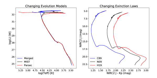
Figure 2: Left: The HR-diagram for a 5 Myr cluster isochrone at solar metallicity using the MergedBaraffePisaEkstromPargisec (blue), MISTv1 (black), and Parsec (red) evolution models. SPISEA allows the user to change evolution models to examine the impact they have on cluster output. Right: The color-magnitude diagram (Keck/NIRC2 J+Kp filters) of a cluster with an extinction of A_Ks = 1.0 mag and distance of 4000 pc, using the Cardelli et al. (1989) law (R_v = 3.1; blue), Nishiyama et al. (2009) law (black), and Hosek et al. (2019b) law (red). The choice of extinction law has a significant impact on the star colors.

The user can select what filters are used for synthetic photometry. A suite of filters comes pre-loaded (Appendix A), and new filters can be added by the user in a relatively straightforward way. The pre-loaded filters span from $\sim$0.3 $\mu$m – 5 $\mu$m and cover a range of telescopes/filter systems (Figure 3).

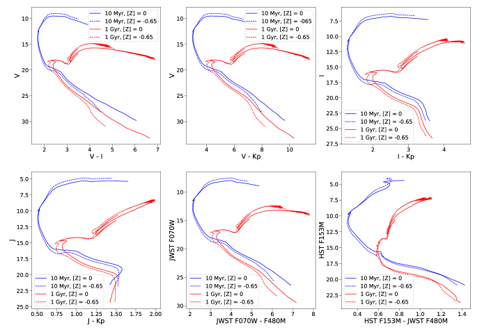
Figure 3: CMDs of a young (10 Myr; blue) and old (1 Gyr; red) cluster isochrone across a range of filters at optical/near-infrared wavelengths. Two metallicities for each age are shown: [Z] = 0 (solar; solid line) and [Z] = -0.65 (dotted line). The isochrones have A_K = 0.5 mag (extinction law from Cardelli et al., 1989) and a distance of 4000 pc. The filters represented are Johnson-Cousins V+I, Keck/NIRC2 J+Kp, HST F153M, and JWST F070W+F480M. The full set of pre-loaded filters can be found in Appendix A, and more can be added by the user.

5.2 SPISEA Clusters

The code required to generate a synthetic cluster is shown in Listing 2. Since SPISEA clusters requires an isochrone object as an input, the user has access to all of the customization options available to the isochrone object in addition to the ability to set the initial mass, IMF, multiplicity, differential extinction, and IFMR.

Listing 2: Making a Synthetic Cluster

⬇

1# Note: the code below assumes that the isochrone

2# has already been created as in Listing 1

3

4# Import necessary packages

5from spisea import synthetic, ifmr

6from spisea.imf import imf, multiplicity

7import numpy as np

8

9# Define stellar multiplicity properties. Here we

10# use the default multiplicity object.

11# If no multiplicity desired, set this variable

12# to None

13imf_multi = multiplicity.MultiplicityUnresolved()

14

15# Define the IFMR. Here we use the default

16# IFMR object.

17# If no IFMR is desired, set this variable

18# to None

19my_ifmr = ifmr.IFMR()

20

21# Define the IMF. Here we’ll use a broken

22# power-law with the parameters from

23# Kroupa et al. (2001, MNRAS, 322, 231),

24# and the multiplicity we defined.

25

26# NOTE: when defining the power law slope

27# for each segment of the IMF, we define

28# the entire exponent, including the negative sign.

29# For example, if dN/dm \propto m^-alpha,

30# then you would use the value -2.3 to specify

31# an IMF with alpha = 2.3.

32

33massLimits = np.array([0.15, 0.5, 1, 120]) # mass segments

34powers = np.array([-1.3, -2.3, -2.3]) # power-law exponents

35my_imf = imf.IMF_broken_powerlaw(massLimits, powers,

36imf_multi)

37

38# Define the initial cluster mass

39mass = 10**5 # Units: solar masses

40

41# Make the cluster object

42cluster = synthetic.ResolvedCluster(my_iso, my_imf, mass,

43ifmr=my_ifmr)

44

45# Access the astropy tables with the properties of

46# the star systems and the individual

47# companion stars.

48# The columns of the table are

49# described in Table 2

50star_systems = cluster.star_systems

51companion_stars = cluster.companions

Figure 4 shows the impact that multiplicity and differential extinction has on the CMD of a star cluster. Both broaden the observed cluster sequence, albeit in different ways. The presence of unresolved multiples makes individual star systems appear brighter and/or redder than their single star counterparts, while differential extinction shifts stars both to the blue and red sides of the average cluster sequence. The unique way that multiplicity broadens the CMD can be used to statistically constrain the multiplicity properties of star clusters, though the impact of differential extinction, photometric errors, and stellar crowding must be considered (e.g. Hu et al., 2010; de Grijs et al., 2013).

The ability to generate clusters with different IMFs has made SPISEA a key component of IMF studies of the Young Nuclear Cluster (Lu et al., 2013) and the Arches Cluster (Hosek et al., 2019b). Figure 5 shows the Kp luminosity function for two identical clusters with different IMFs, one with a “standard” IMF of Kroupa (2001) and the other with a top-heavy IMF (e.g, a relative overabundance of high-mass stars) similar to Hosek et al. (2019b). With SPISEA, one can examine how the stellar population and compact remnants are expected to change with the IMF. Figure 5 also includes the black hole mass function for both IMFs, as defined by the default IFMR object.

One can also assess the impact of different evolution and atmosphere models on a simulated star cluster by changing the isochrone that is used. For example, the number ratio of massive Wolf-Rayet (WR) stars to other types of stars is a useful age indicator for a population (e.g. Meynet et al., 1994), though it can be affected by metallicity, stellar rotation, and binary star evolution (e.g. Ekström et al., 2012; Georgy et al., 2012; Dorn-Wallenstein & Levesque, 2018). SPISEA allows the user to examine how differences between evolution models impacts these predictions (Figure 6). Note that SPISEA does not yet distinguish between different sub-classes of WR stars, such as WC and WN stars.

In addition, SPISEA has the ability to sum the spectra of the individual stars to make a composite spectrum of the stellar population (Figure 7). This can be used to analyze unresolved stellar populations. However, note that there is no treatment of nebular emission, which can have a significant impact on observations of very young clusters which remain enshrouded in leftover gas and dust leftover from formation (e.g. Mollá et al., 2009; Reines et al., 2010). In addition, SPISEA uses stellar atmospheres that assume local thermodynamic equilibrium (LTE), an assumption that breaks down for the most massive stars, which can dominate a composite spectrum. Implementing non-LTE atmospheres is a priority in future code development ($\mathsection$6), though the user can implement additional atmospheres of their choosing with the current release.

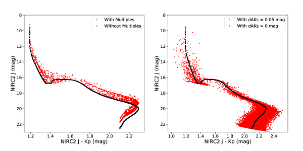
Figure 4: Left: A SPISEA cluster generated with (red) and without (black) the multiplicity as described by Lu et al. (2013). The presence of multiples generally makes star systems appear brighter and redder than single stars. Right: A SPISEA cluster with differential extinction applied (dA_Ks = 0.05 mag; red) versus one without (black). No multiple systems are included in order to isolate the impact of differential extinction on the CMD. For all isochrones, the MISTv1 evolution models are used with the get_merged_atmospheres atmosphere models.

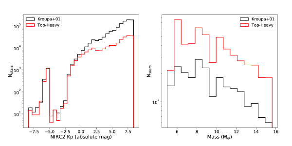
Figure 5: Left: NIRC2 Kp luminosity function of two clusters (10⁶ M_⊙, 100 Myr, [Z] = 0), one from Kroupa (2001, black) and the other with the top-heavy IMF from Hosek et al. (2019b, red). For a given total mass, the top-heavy IMF has a larger fraction of high-mass stars to low-mass stars relative to the Kroupa IMF. Right: The black hole mass function for the two clusters, with the Kroupa IMF in black and top-heavy IMF in red. The top-heavy IMF produces more black holes than the Kroupa IMF, especially at higher masses.

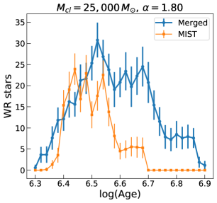
Figure 6: Number of WR stars in synthetic clusters over different ages generated by SPISEA with MergedBaraffePisaEkstromParsec and MISTv1 evolution models, given the cluster mass ($M_{cl}=25,000M_{\odot}$) and IMF slope ($\alpha$ = 1.80).

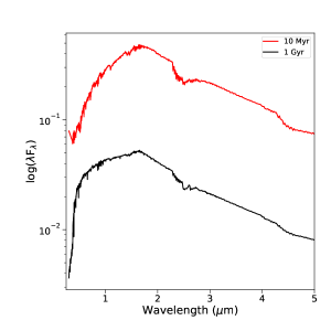
Figure 7: Unresolved near-infrared spectra of a young (10 Myr, red) and old (1 Gyr, black) cluster. The young cluster is generated with an initial mass of 5x10³ M_⊙, while the old cluster has an initial mass of 5x10⁴ M_⊙. The differences in the composite spectra are driven by the differences in the stellar populations, in particular the presence of high-mass stars in the young population.

5.3 Comparing to Observations

Hosek et al. (2019b) use SPISEA to compare the observed CMD of the Arches Cluster to synthetic color-magnitude diagrams of model clusters with different input properties. As an additional demonstration, Figure 8 compares the observed 2MASS CMD of the Praesepe Cluster (M44) to a SPISEA cluster with the best-fit properties from the literature. The observed data contain cluster candidates with M $\gtrsim$ 0.3 M_⊙ identified via kinematic and photometric properties by Wang et al. (2014). We adopt the following properties for the synthetic cluster: age = 590 Myr (Gossage et al., 2018), A_K = 0 mag (Taylor, 2006, measure A_v = 0.08 mag, which is negligible at K-band), distance = 179 pc (Gáspár et al., 2009), [Z] = 0 (Boesgaard et al., 2013, obtain a slightly super-solar metallicity for M44, but solar metallicity is the closest in the grid of MIST models currently available in SPISEA), and a standard Kroupa IMF (Boudreault et al., 2012). We adopt the default MultiplicityUnresolved object ($\mathsection$4.1) for the multiplicity properties of the cluster, and use the MIST stellar evolution models and get_merged_atmosphere atmosphere models to generate the synthetic stars. We simulate photometric errors by perturbing the synthetic photometry of each star by a random amount drawn from the typical photometric uncertainty of the observations (0.02 mags). We see that the SPISEA CMD is a generally good match to the observations, though a detailed analysis is beyond the scope of this paper.

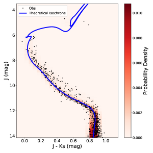
Figure 8: A comparison of the observed 2MASS CMD of M44 (Wang et al., 2014) to a SPISEA cluster generated using the best-fit values from the literature. The observed cluster candidates are represented by the black points (typical uncertainty: 0.02 mags) and the theoretical isochrone by the blue line. The CMD is shaded according to the probability density distribution of the stars in the synthetic cluster. The SPISEA cluster provides a generally good match to the observed data.

5.4 Code Performance

When simulating a cluster with SPISEA, the majority of the computation time is spent calculating synthetic photometry in the isochrone. On an 3 GHz Intel Xenon processor, the time required to compute an isochrone from scratch is $\sim$1 – 5 mins, depending on the age of the cluster, the evolution/atmosphere models used and number of photometric filters chosen. However, once the isochrone is generated, the process of building the cluster is fast: one can make a ResolvedCluster object with an initial mass of 10⁴ M_⊙ in $\sim$1 s. Thus, after pre-generating a grid of isochrones, one can quickly build many clusters with different properties within likelihood functions for forward modeling purposes.

Building an UnresolvedCluster object is more time intensive, since the process of assigning spectra to each star in the cluster is relatively slow. One can make an unresolved cluster with an initial mass of 10⁴ M_⊙ cluster with a Kroupa (2001) IMF in $\sim$15 s.

6 SPISEA Limitations and Future Development

The first release of the SPISEA code has several limitations that present opportunities for future code development. Some of these limitations require relatively straightforward adjustments to the current code, and will be addressed in future code releases:

• Very Hot Star Models: All of the stellar atmosphere models that are pre-loaded into SPISEA assume LTE, an assumption that breaks down for the most massive stars. This is especially true for Wolf-Rayet stars, which have extreme stellar winds that must be accounted for (e.g. Hillier & Miller, 1998; Gräfener et al., 2002). While the user has the flexibility to add their own hot star atmospheres in the short term, we plan to implement them among the pre-loaded atmospheres in the long term.

• Very Cool Star Models: The pre-loaded SPISEA evolution models stretch to the brown-dwarf limit at 0.08 M_⊙ (via the models from Baraffe et al., 2015), but do not extend into the brown dwarf regime. In addition, the lowest temperature atmospheres only extend to 1200 K. Similar to the very hot star models, very cool star models can be implemented individually by the user, but ideally they would be included in the base package in the future.

• Additional Metallicity Support: Currently, the only non-solar stellar evolution models that comes with SPISEA is from MIST (Choi et al., 2016). However, other non-solar metallicity models exist, for example from the Geneva group for main sequence/post-main sequence stars (e.g. Georgy et al., 2013) and the Pisa group for pre-main sequence stars (Tognelli et al., 2011). These can be implemented by the user for now, and will be pre-loaded in future code releases.

• Additional IMF Functional Forms: SPISEA offers the user full control in defining an IMF with a broken power-law functional form ($\mathsection$4.2). However, a log-normal functional form has been proposed for M $\lesssim$ 1 M_⊙, with a power-law for M $\gtrsim$ 1 M_⊙ (e.g. Chabrier, 2003). While the true functional form of the IMF is not yet clear, improved observational facilities will allow for IMF measurements at the low masses necessary to distinguish between these two functional forms (e.g. El-Badry et al., 2017; Hosek et al., 2019a). Thus, implementation of the log-normal form of the IMF will be very useful for future analyses. This will be included in future code releases, but can be implemented by the user in the meantime.

• Complex Star Formation Histories: Currently, SPISEA only produces SSPs and is not equipped to produce a composite stellar population with a distribution of ages or metallicities. While most star clusters are assumed to be SSPs, recent work shows this assumption may not be valid for globular clusters (e.g. Piotto et al., 2015), and certainly more complex star formation histories are required to model galaxy-wide stellar populations. While it straightforward to approximate a composite population by combining a series of individual SSPs (e.g. Bruzual & Charlot, 2003; Lam et al., 2020), implementing a star formation history module within the code itself is an avenue for future work.

In addition, future releases of SPISEA will also have new and updated stellar evolution and atmosphere models, IFMRs, and multiplicity properties pre-loaded as they become available.

Addressing other limitations will require more substantial code development:

• Binary Star Evolution: While SPISEA has a treatment for unresolved stellar multiplicity ($\mathsection$4.1), only single star stellar evolution models are available in the pre-loaded set. However, it has been found that interactions between binary stars can have a significant impact on stellar evolution, particularly for high-mass stars (e.g. Hurley et al., 2002; Eldridge et al., 2017; Dorn-Wallenstein & Levesque, 2018). SPISEA does not yet produce orbital properties of multiple systems (e.g. orbital periods and eccentricities), and so interactions cannot be modeled. In addition, modeling binary interactions is computationally intensive, and so a major expansion of the current code or an interface with an existing binary evolution codes would be required.

• Theoretical Dust Extinction and Nebular Emission: SPISEA does not include any radiative transfer or photoionization calculations, and so theoretical dust extinction curves and nebular emission cannot be calculated within the code. Instead, the user is required to do such calculations outside of SPISEA and implement their own extinction law objects as desired. Designing an interface between SPISEA and existing radiative transfer codes such as cloudy (Ferland et al., 2013) would be a significant undertaking, but can be explored if there is interest.

7 User Contributions

We encourage community input and contributions to SPISEA through the GitHub page given in $\mathsection$1. Any bugs, questions, or feature requests should be reported via the issue tracker. If the user wishes to add features themselves, we ask that they fork or branch off of the current development repository, make their changes, and then submit merge and pull requests. The contributions will be added (and attribution given) in future releases of the code.

8 Conclusions

We introduce SPISEA, an open-source Python code to generate SSPs. The modular interface of SPISEA offers unparalleled flexibility in defining the IMF, IFMR, extinction law, stellar multiplicity properties, and the stellar evolution and atmosphere model grids used to generate synthetic star clusters. Example code outputs include cluster color-magnitude diagrams in a multitude of filters (also defined by the user), HR-diagrams, stellar mass functions, and compact object populations. SPISEA is available on GitHub and ReadtheDocs. We encourage input and contributions from the community.

Appendix A Pre-Loaded SPISEA Options

Here we describe the set of pre-loaded models in the initial release of SPISEA. The set of evolution and and atmosphere model grids is shown in Table 3, extinction laws in Table 4, and photometric filters in Table 5. Additional models can be added by the user.

Table 3: Evolution and Atmosphere Models

Evolution Models
Model Name	Mass Range	log(Age) Range	Metallicity Range			Ref
	M⊙	Years	[Fe/H]
MIST v1.2	0.1 – 300	6.0 – 10.01	-4.0 – 0.5			Choi et al. (2016)
MergedBaraffePisaEkstromParsec	0.08 – 120	6.0 – 10.09	0			see Appendix B
Parsec	0.1 – 65	6.6 – 10.12	0			Bressan et al. (2012)
Baraffe15	0.07 – 1.4	5.7 – 10.0	0			Baraffe et al. (2015)
Ekstrom12	0.8 – 300	6.0 – 8.0	0			Ekström et al. (2012)
Pisa	0.2 – 7	6.0 – 8.0	0			Tognelli et al. (2011)
Atmosphere Models
Model Name	Teff Range	log $g$ Range	Metallicity Range	$\lambda$ Range	Resolution	Ref
	K	cgs	[Fe/H]	$\mu$m	$\lambda$ / $\Delta\lambda$
get_merged_atmosphere	3200 – 50000	b	b	b	b	see Appendix B
get_castelli_atmosphere	3500 – 50000	0 – 5.0	-2.5 – 0.2	0.1 – 10	$\sim$250	Castelli & Kurucz (2004)
get_phoenixv16_atmosphere	2300 – 12000	0.0 – 6.0	-4.0 – +1.0	0.05 – 5.5	100,000 – 500,000	Husser et al. (2013)
get_BTSettl_2015_atmosphere	1200 – 7000	2.5 – 5.5	0	0.01 – 30	2000 – 700,000	Baraffe et al. (2015)
get_BTSettl_atmosphere	2600 – 7000	4.5 – 5.5	-2.5 – 0.5	0.1 – 6.9	20,000 – 250,000	Allard et al. (2012b, a)
get_kurucz_atmosphere	3000 — 50000	0 – 5.0	-5.0 – 1.0	0.1 – 10	$\sim$250	c
get_phoenix_atmosphere	2100 – 69000		-4.0 – 0.5	0.001 – 995	$\sim$280	Allard et al. (2003, 2007)
get_wd_atmosphere	–	–	–	0.1 – 3.0	200 – 500,000	Koester (2010)

Table 4: Extinction Laws

Name	$\lambda_{0}$	$\lambda$ Range	User Inputs	Ref
	$\mu$m	$\mu$m
RedLawReikeLebofsky	2.12	0.365 - 13.0		Rieke & Lebofsky (1985)
RedLawCardelli	2.174	0.3 – 3.0	R(V)	Cardelli et al. (1989)
RedLawRomanZuniga07	2.134	1.24 – 7.76		Román-Zúñiga et al. (2007)
RedLawFitzpatrick09	2.14	0.7 – 3.0	$\alpha$, R(V)	Fitzpatrick & Massa (2009)
RedLawNishiyama09	2.14	0.5 – 8.0		Nishiyama et al. (2008, 2009)
RedLawFritz11	2.14	1.0 – 19.0		Fritz et al. (2011)
RedLawDamineli16	2.159	0.44 – 4.48		Damineli et al. (2016)
RedLawSchlafly16	2.14	0.5 – 4.8	AH / AKs, x	Schlafly et al. (2016)
RedLawHosek18	2.14	0.7 – 3.545		Hosek et al. (2018)
RedLawHosek18b	2.14	0.7 – 3.545		Hosek et al. (2019b)
RedLawNoguerasLara18	2.15	0.8 – 2.8		Nogueras-Lara et al. (2018)
RedLawPowerLaw	—	—	$\alpha$, $\lambda_{0}$	—

Table 5: Photometric Filters

Telescope/System	Filters	Ref
2MASS	J, H, Ks	Cohen et al. (2003)
CTIO/OSIRIS	H, K	1
DeCam	u, g, r, i, z, Y	Abbott et al. (2018)
Gaia	G, Gbp, Grp	Evans et al. (2018)
Hubble Space Telescope	see pysynphot documentation	–
Johnson-Cousins	U, B, V, R, I	Johnson et al. (1966)
Johnson-Glass	J, H, K	Bessell & Brett (1988)
James Webb Space Telescope/NIRCAM	see website	2
Keck/NIRC	H, K	3
Keck/NIRC2	J, H, Hcont, K, Kp, Ks, Kcont,
	Lp, Ms, Brgamma, FeII	4
NACO	J, H, K	5
PanStarrs 1	g, r, i, z, y	Tonry et al. (2012)
UKIRT	J, H, K	Hewett et al. (2006)
VISTA	Z, Y, J, H, K	6

Appendix B Description of Merged Evolution and Atmosphere Models

SPISEA comes with one set of merged stellar evolution models and one set of merged stellar atmosphere models. These are created in order to take advantage of the strengths of different model sets in different parameter spaces, such as different stellar masses, temperatures, population ages, evolutionary stage, etc. These merged grids are currently only available at solar metallicities.

The merged stellar evolution object is evolution.MergedBaraffePisaEkstromParsec. It is comprised of 4 recent stellar evolution models: Baraffe15 (Baraffe et al., 2015), Pisa (Tognelli et al., 2011), Ekstrom/Geneva (both with and without rotation; Ekström et al., 2012), and Parsec v1.2 (Bressan et al., 2012). Which models are used depends on the population age. If logAge $<$ 7.4, then Baraffe15 is used for 0.08 M_⊙ – 0.4 M_⊙, Pisa is used from 0.5 M_⊙ to the highest mass available (typically between 5 – 7 M_⊙), and the Ekstrom/Geneva models are used from the highest mass in the Pisa models to 120 M_⊙. In the transition region between 0.4 M_⊙ – 0.5 M${\odot}$, a linear interpolation between the Baraffe15 and Pisa models is used. If logAge $>$ 7.4, Parsec v1.2 is used for the full mass range.

This merged method was chosen to emphasize the strengths of the different models. For example, the Ekstrom/Geneva grid offers coverage of young main sequence and post-main sequence stars, but does not include the pre-main sequence. Meanwhile, the combination of the Pisa and Baraffe15 grids offer coverage of young pre-main sequence stars down to the hydrogen burning limit. Additionally, Parsec is well suited for old star populations, where the Ekstrom/Geneva grid only covers ages up to 100 Myr.

The merged stellar atmosphere grid is defined by the atmospheres.get_merged_atmospheres object. It contains a mix of ATLAS9 (Castelli & Kurucz, 2004), PHOENIX v16 (Husser et al., 2013), BTSettl (Baraffe et al., 2015), and Koester10 (Koester, 2010) atmospheres. It is described in $\mathsection$2.2 of Lam et al. (2020). Briefly, which atmosphere grid is used depends on the stellar temperature and evolutionary state. For stars, the ATLAS9 grid is used for stars with T_eff $>$ 5500 K, the PHOENIX grid is used for 5000 K $<$ T_eff $<$ 3800 K, and the BTSettl grid is used for 3200 K $<$ T_eff $<$ 1200 K. For temperatures at transition temperatures between grids (e.g. 5000 K – 5500 K), an average atmosphere between the two model grids is used. For white dwarfs with known physical properties (i.e., those included in the MISTv1 evolution models), the Koester10 atmospheres are used. If the white dwarf properties lie outside the Koester10 model grid, then a blackbody curve is used instead.

References

- Abbott et al. (2018) Abbott, T. M. C., Abdalla, F. B., Allam, S., et al. 2018, ApJS, 239, 18
- Allard et al. (2007) Allard, F., Allard, N. F., Homeier, D., et al. 2007, A&A, 474, L21
- Allard et al. (2003) Allard, F., Guillot, T., Ludwig, H.-G., et al. 2003, in IAU Symposium, Vol. 211, Brown Dwarfs, ed. E. Martín, 325
- Allard et al. (2012a) Allard, F., Homeier, D., & Freytag, B. 2012a, Philosophical Transactions of the Royal Society of London Series A, 370, 2765
- Allard et al. (2012b) Allard, F., Homeier, D., Freytag, B., & Sharp, C. M. 2012b, in EAS Publications Series, Vol. 57, EAS Publications Series, ed. C. Reylé, C. Charbonnel, & M. Schultheis, 3–43
- Andersen et al. (2017) Andersen, M., Gennaro, M., Brandner, W., et al. 2017, A&A, 602, A22
- Astropy Collaboration et al. (2013) Astropy Collaboration, Robitaille, T. P., Tollerud, E. J., et al. 2013, A&A, 558, A33
- Astropy Collaboration et al. (2018) Astropy Collaboration, Price-Whelan, A. M., Sipőcz, B. M., et al. 2018, AJ, 156, 123
- Baraffe et al. (2015) Baraffe, I., Homeier, D., Allard, F., & Chabrier, G. 2015, A&A, 577, A42
- Bastian et al. (2010) Bastian, N., Covey, K. R., & Meyer, M. R. 2010, ARA&A, 48, 339
- Bessell & Brett (1988) Bessell, M. S., & Brett, J. M. 1988, PASP, 100, 1134
- Boesgaard et al. (2013) Boesgaard, A. M., Roper, B. W., & Lum, M. G. 2013, ApJ, 775, 58
- Boudreault et al. (2012) Boudreault, S., Lodieu, N., Deacon, N. R., & Hambly, N. C. 2012, MNRAS, 426, 3419
- Bressan et al. (2012) Bressan, A., Marigo, P., Girardi, L., et al. 2012, MNRAS, 427, 127
- Bruzual & Charlot (2003) Bruzual, G., & Charlot, S. 2003, MNRAS, 344, 1000
- Burki (1975) Burki, G. 1975, A&A, 43, 37
- Cardelli et al. (1989) Cardelli, J. A., Clayton, G. C., & Mathis, J. S. 1989, ApJ, 345, 245
- Castelli & Kurucz (1994) Castelli, F., & Kurucz, R. L. 1994, A&A, 281, 817
- Castelli & Kurucz (2004) —. 2004, ArXiv Astrophysics e-prints, astro-ph/0405087
- Cerviño (2013) Cerviño, M. 2013, New A Rev., 57, 123
- Chabrier (2003) Chabrier, G. 2003, PASP, 115, 763
- Chen et al. (2019) Chen, Z., Gallego-Cano, E., Do, T., et al. 2019, ApJ, 882, L28
- Choi et al. (2016) Choi, J., Dotter, A., Conroy, C., et al. 2016, ApJ, 823, 102
- Cohen et al. (2003) Cohen, M., Wheaton, W. A., & Megeath, S. T. 2003, AJ, 126, 1090
- Conroy & Gunn (2010) Conroy, C., & Gunn, J. E. 2010, FSPS: Flexible Stellar Population Synthesis, Astrophysics Source Code Library, , , ascl:1010.043
- Conroy et al. (2009) Conroy, C., Gunn, J. E., & White, M. 2009, ApJ, 699, 486
- da Silva et al. (2012) da Silva, R. L., Fumagalli, M., & Krumholz, M. 2012, ApJ, 745, 145
- Damineli et al. (2016) Damineli, A., Almeida, L. A., Blum, R. D., et al. 2016, MNRAS, 463, 2653
- de Grijs et al. (2013) de Grijs, R., Li, C., Zheng, Y., et al. 2013, ApJ, 765, 4
- Dorn-Wallenstein & Levesque (2018) Dorn-Wallenstein, T. Z., & Levesque, E. M. 2018, ApJ, 867, 125
- Duchêne & Kraus (2013) Duchêne, G., & Kraus, A. 2013, ARA&A, 51, 269
- Ekström et al. (2012) Ekström, S., Georgy, C., Eggenberger, P., et al. 2012, A&A, 537, A146
- El-Badry et al. (2017) El-Badry, K., Weisz, D. R., & Quataert, E. 2017, MNRAS, 468, 319
- Eldridge et al. (2017) Eldridge, J. J., Stanway, E. R., Xiao, L., et al. 2017, PASA, 34, e058
- Evans et al. (2018) Evans, D. W., Riello, M., De Angeli, F., et al. 2018, A&A, 616, A4
- Ferland et al. (2013) Ferland, G. J., Porter, R. L., van Hoof, P. A. M., et al. 2013, Rev. Mexicana Astron. Astrofis., 49, 137
- Fioc & Rocca-Volmerange (1997) Fioc, M., & Rocca-Volmerange, B. 1997, A&A, 500, 507
- Fioc & Rocca-Volmerange (2019) —. 2019, A&A, 623, A143
- Fitzpatrick & Massa (2009) Fitzpatrick, E. L., & Massa, D. 2009, ApJ, 699, 1209
- Fritz et al. (2011) Fritz, T. K., Gillessen, S., Dodds-Eden, K., et al. 2011, ApJ, 737, 73
- Gáspár et al. (2009) Gáspár, A., Rieke, G. H., Su, K. Y. L., et al. 2009, ApJ, 697, 1578
- Georgy et al. (2013) Georgy, C., Ekström, S., Granada, A., et al. 2013, A&A, 553, A24
- Georgy et al. (2012) Georgy, C., Ekström, S., Meynet, G., et al. 2012, A&A, 542, A29
- Georgy et al. (2014) Georgy, C., Granada, A., Ekström, S., et al. 2014, A&A, 566, A21
- Girardi et al. (2002) Girardi, L., Bertelli, G., Bressan, A., et al. 2002, A&A, 391, 195
- Gossage et al. (2018) Gossage, S., Conroy, C., Dotter, A., et al. 2018, ApJ, 863, 67
- Gräfener et al. (2002) Gräfener, G., Koesterke, L., & Hamann, W.-R. 2002, A&A, 387, 244
- Habibi et al. (2013) Habibi, M., Stolte, A., Brandner, W., Hußmann, B., & Motohara, K. 2013, A&A, 556, A26
- Hatton et al. (2003) Hatton, S., Devriendt, J. E. G., Ninin, S., et al. 2003, MNRAS, 343, 75
- Heger et al. (2003) Heger, A., Fryer, C. L., Woosley, S. E., Langer, N., & Hartmann, D. H. 2003, ApJ, 591, 288
- Hewett et al. (2006) Hewett, P. C., Warren, S. J., Leggett, S. K., & Hodgkin, S. T. 2006, MNRAS, 367, 454
- Hillier & Miller (1998) Hillier, D. J., & Miller, D. L. 1998, ApJ, 496, 407
- Hosek et al. (2019a) Hosek, M., Lu, J. R., Andersen, M., et al. 2019a, in BAAS, Vol. 51, Bulletin of the American Astronomical Society, 439
- Hosek et al. (2015) Hosek, Jr., M. W., Lu, J. R., Anderson, J., et al. 2015, ApJ, 813, 27
- Hosek et al. (2019b) —. 2019b, ApJ, 870, 44
- Hosek et al. (2018) —. 2018, ApJ, 855, 13
- Hu et al. (2010) Hu, Y., Deng, L., de Grijs, R., Liu, Q., & Goodwin, S. P. 2010, ApJ, 724, 649
- Hurley et al. (2002) Hurley, J. R., Tout, C. A., & Pols, O. R. 2002, MNRAS, 329, 897
- Husser et al. (2013) Husser, T.-O., Wende-von Berg, S., Dreizler, S., et al. 2013, A&A, 553, A6
- Johnson et al. (1966) Johnson, H. L., Mitchell, R. I., Iriarte, B., & Wisniewski, W. Z. 1966, Communications of the Lunar and Planetary Laboratory, 4, 99
- Kalirai et al. (2008) Kalirai, J. S., Hansen, B. M. S., Kelson, D. D., et al. 2008, ApJ, 676, 594
- Kim et al. (2005) Kim, S. S., Figer, D. F., Lee, M. G., & Oh, S. 2005, PASP, 117, 445
- Koester (2010) Koester, D. 2010, Mem. Soc. Astron. Italiana, 81, 921
- Krishna Gautam et al. (2019) Krishna Gautam, A., Do, T., Ghez, A. M., et al. 2019, ApJ, 871, 103
- Kroupa (2001) Kroupa, P. 2001, MNRAS, 322, 231
- Krumholz et al. (2015) Krumholz, M. R., Fumagalli, M., da Silva, R. L., Rendahl, T., & Parra, J. 2015, MNRAS, 452, 1447
- Lam et al. (2020) Lam, C. Y., Lu, J. R., Hosek, Matthew W., J., Dawson, W. A., & Golovich, N. R. 2020, ApJ, 889, 31
- Leitherer et al. (1999) Leitherer, C., Schaerer, D., Goldader, J. D., et al. 1999, ApJS, 123, 3
- Lu et al. (2013) Lu, J. R., Do, T., Ghez, A. M., et al. 2013, ApJ, 764, 155
- Maraston (1998) Maraston, C. 1998, MNRAS, 300, 872
- Maraston (2005) —. 2005, MNRAS, 362, 799
- Maraston et al. (2020) Maraston, C., Hill, L., Thomas, D., et al. 2020, MNRAS, arXiv:1911.05748
- Meynet et al. (1994) Meynet, G., Maeder, A., Schaller, G., Schaerer, D., & Charbonnel, C. 1994, A&AS, 103, 97
- Miller & Scalo (1979) Miller, G. E., & Scalo, J. M. 1979, ApJS, 41, 513
- Moe & Di Stefano (2017) Moe, M., & Di Stefano, R. 2017, ApJS, 230, 15
- Mollá et al. (2009) Mollá, M., García-Vargas, M. L., & Bressan, A. 2009, MNRAS, 398, 451
- Nataf et al. (2016) Nataf, D. M., Gonzalez, O. A., Casagrande, L., et al. 2016, MNRAS, 456, 2692
- Nishiyama et al. (2008) Nishiyama, S., Nagata, T., Tamura, M., et al. 2008, ApJ, 680, 1174
- Nishiyama et al. (2009) Nishiyama, S., Tamura, M., Hatano, H., et al. 2009, ApJ, 696, 1407
- Nogueras-Lara et al. (2019) Nogueras-Lara, F., Schödel, R., Najarro, F., et al. 2019, arXiv e-prints, arXiv:1909.02494
- Nogueras-Lara et al. (2018) Nogueras-Lara, F., Gallego-Calvente, A. T., Dong, H., et al. 2018, A&A, 610, A83
- Noll et al. (2009) Noll, S., Burgarella, D., Giovannoli, E., et al. 2009, A&A, 507, 1793
- Pflamm-Altenburg & Kroupa (2006) Pflamm-Altenburg, J., & Kroupa, P. 2006, MNRAS, 373, 295
- Piotto et al. (2015) Piotto, G., Milone, A. P., Bedin, L. R., et al. 2015, AJ, 149, 91
- Portinari et al. (1998) Portinari, L., Chiosi, C., & Bressan, A. 1998, A&A, 334, 505
- Raithel et al. (2018) Raithel, C. A., Sukhbold, T., & Özel, F. 2018, ApJ, 856, 35
- Reines et al. (2010) Reines, A. E., Nidever, D. L., Whelan, D. G., & Johnson, K. E. 2010, ApJ, 708, 26
- Reipurth & Zinnecker (1993) Reipurth, B., & Zinnecker, H. 1993, A&A, 278, 81
- Rieke & Lebofsky (1985) Rieke, G. H., & Lebofsky, M. J. 1985, ApJ, 288, 618
- Román-Zúñiga et al. (2007) Román-Zúñiga, C. G., Lada, C. J., Muench, A., & Alves, J. F. 2007, ApJ, 664, 357
- Rui et al. (2019) Rui, N. Z., Hosek, Matthew W., J., Lu, J. R., et al. 2019, ApJ, 877, 37
- Salpeter (1955) Salpeter, E. E. 1955, ApJ, 121, 161
- Sana et al. (2012) Sana, H., de Mink, S. E., de Koter, A., et al. 2012, Science, 337, 444
- Schlafly et al. (2016) Schlafly, E. F., Meisner, A. M., Stutz, A. M., et al. 2016, ApJ, 821, 78
- Schödel et al. (2010) Schödel, R., Najarro, F., Muzic, K., & Eckart, A. 2010, A&A, 511, A18
- Stanway & Eldridge (2018) Stanway, E. R., & Eldridge, J. J. 2018, MNRAS, 479, 75
- Stevance et al. (2020) Stevance, H., Eldridge, J., & Stanway, E. 2020, The Journal of Open Source Software, 5, 1987
- STScI Development Team (2013) STScI Development Team. 2013, pysynphot: Synthetic photometry software package, Astrophysics Source Code Library, , , ascl:1303.023
- Sukhbold et al. (2016) Sukhbold, T., Ertl, T., Woosley, S. E., Brown, J. M., & Janka, H. T. 2016, ApJ, 821, 38
- Sukhbold et al. (2018) Sukhbold, T., Woosley, S. E., & Heger, A. 2018, ApJ, 860, 93
- Taylor (2006) Taylor, B. J. 2006, AJ, 132, 2453
- Tognelli et al. (2011) Tognelli, E., Prada Moroni, P. G., & Degl’Innocenti, S. 2011, A&A, 533, A109
- Tonry et al. (2012) Tonry, J. L., Stubbs, C. W., Lykke, K. R., et al. 2012, ApJ, 750, 99
- Vázquez & Leitherer (2005) Vázquez, G. A., & Leitherer, C. 2005, ApJ, 621, 695
- Wang et al. (2014) Wang, P. F., Chen, W. P., Lin, C. C., et al. 2014, ApJ, 784, 57
- Wang & Chen (2019) Wang, S., & Chen, X. 2019, ApJ, 877, 116
- Wang & Jiang (2014) Wang, S., & Jiang, B. W. 2014, ApJ, 788, L12
- Weidner & Kroupa (2004) Weidner, C., & Kroupa, P. 2004, MNRAS, 348, 187
- Xiao et al. (2018) Xiao, L., Stanway, E. R., & Eldridge, J. J. 2018, MNRAS, 477, 904