STRATIFY: a comprehensive and versatile MATLAB code for a multilayered sphere

Abstract

We present a computer code for calculating near- and far-field electromagnetic properties of multilayered spheres. STRATIFY is one-of-a-kind open-source package which allows for the efficient calculation of electromagnetic near-field, energy density, total electromagnetic energy, radiative and non-radiative decay rates of a dipole emitter located in any (non-absorbing) shell (including a host medium), and fundamental cross-sections of a multilayered sphere, all within a single program. The developed software is typically more than $50$ times faster than freely available packages based on boundary-element-method. Because of its speed and broad applicability, our package is a valuable tool for analysis of numerous light scattering problems, including, but not limited to fluorescence enhancement, upconversion, downconversion, second harmonic generation, surface enhanced Raman spectroscopy. The software is available for download from GitLab https://gitlab.com/iliarasskazov/stratify.

1 Introduction

Multilayered spherical nanoparticles are fundamental building blocks for many vital applications in physics and chemistry: tailored scattering  [1, 2, 3, 4, 5, 6, 7] and nonlinear optics [1, 2, 8, 9], photonic crystals [10, 11, 12, 13, 14], sensing [15, 16, 17], photothermal cancer treatment [18, 19, 20, 21], solar energy harvesting [22, 23], photovoltaics [24], fluorescence [25, 26, 27, 28, 29, 30], photoluminescence [31] and upconversion [32, 33, 34, 35, 36, 37, 38, 39, 40] enhancement, surface-enhanced Raman scattering (SERS) [25, 41, 42], surface plasmon amplification by stimulated emission of radiation (spaser) [43, 44, 45, 46, 47, 48], and cloaking [49, 50, 51, 52]. To date, such matryoshkas with various combinations of dielectric and metal shells have well-established protocols for the efficient and controllable synthesis [6, 53, 54, 55, 56, 57], greatly improved on initial synthesis attempts [3, 4, 5]. Theoretical and numerical studies in these fields are inevitable for a thoughtful design of experiment and reliable interpretation of measured data. The theory of electromagnetic light scattering from multilayered spheres has a long history since the pioneering work of Aden and Kerker for two concentric spheres [58]. An impressive number of closed-form solutions and discussions on coated [59, 60] and general multilayered [61] spheres have been reported. There is a thorough understanding of scattering [62] and absorption [63] of light from multilayered spheres, including aspects for various types of illuminations [64, 65, 66, 67], spontaneous decay rates of a dipole emitter in a presence of a multilayered sphere [68, 69], electromagnetic energy [70] and near-field [71] distribution within and near the multilayered spheres, and the respective strategies for numerical implementation of the developed theories [72, 73, 74, 75].

For a single shell, a number of features can be qualitatively understood from the quasi-static analysis [2], a full, quantitative understanding of the mechanisms underlying the applications of multilayered spheres is usually quite involved, requiring sophisticated and complex theoretical and numerical studies. The latter are often handled with commercial brute-force finite-difference time-domain (FDTD), finite-element-method (FEM) or boundary-element-method (BEM) solvers, which provide accurate results at relatively high computational price. However, spherical multilayered particles are computationally feasible per se due to the existence of the closed-form analytical solutions inherently convenient for computational implementation. Nonetheless, there are few freely available, user-friendly and comprehensive codes for light scattering from a general multilayered spheres based on these solutions [76]. In most of the cases, a very limited number of properties are calculated within a single freely available package. Fundamental cross-sections (i.e. scattering, absorption and extinction) and/or near fields are the usual choice implemented in freely available codes [77, 78], and in a number of so-called “online Mie calculators”, which commonly handle only homogeneous spheres with a rare exceptions for core-shells and even more rarely for general multilayered spheres. Computation of the orientation-averaged electric or magnetic field intensities (i.e. averaged over a spherical surface of a given fixed radius $r$), spontaneous decay rates and other quantities are almost unavailable, yet generally very useful. Here we present free MATLAB code based on compact and easy-to-implement transfer-matrix formalism, which can be conveniently used to handle most of the problems of light scattering from multilayered spheres by using appropriate combinations and manipulations of transfer-matrices. The use of closed-form solutions significantly enhances the performance of the code compared with brute-force solvers without sacrificing the accuracy.

Our recursive transfer-matrix method (RTMM) has been inspired by the success of such a RTMM for planar stratified media developed by Abelès [79, 80, 81], summarized in Born & Wolf classical textbook [82, Sec.1.6], and can be seen as its analogue for spherical interfaces. From a historical perspective, the RTMM presented here had been developed as early as in 1998 and implemented in the F77 sphere.f code [76]. It was first applied to a number of different theoretical settings with external plane wave source [10, 12, 14], and successfully tested against experiment [13, 6]. Later it was extended to incorporate a dipole source [68, 69], energy calculations [70], and has enabled exhaustive optimization of plasmon-enhanced fluorescence [30].

The paper is organized as follows. In Sec. 2, we provide an overview of the RTMM for multilayered spheres and formulate the fundamental properties of spheres. In Sec. 3, we describe the developed code and benchmark it with robust BEM [83] implemented in freely available “MNPBEM” MATLAB package [84, 85, 86, 87]. In Sec. 4, we discuss possible application of the code in SERS, plasmon-enhanced fluorescence, upconversion, and end with conclusive remarks and propose further developments of the package. Gaussian units are used throughout the paper.

2 Theory

2.1 Recursive Transfer-Matrix method

Consider a multilayered sphere with $N$ concentric shells as shown in Fig. 1.

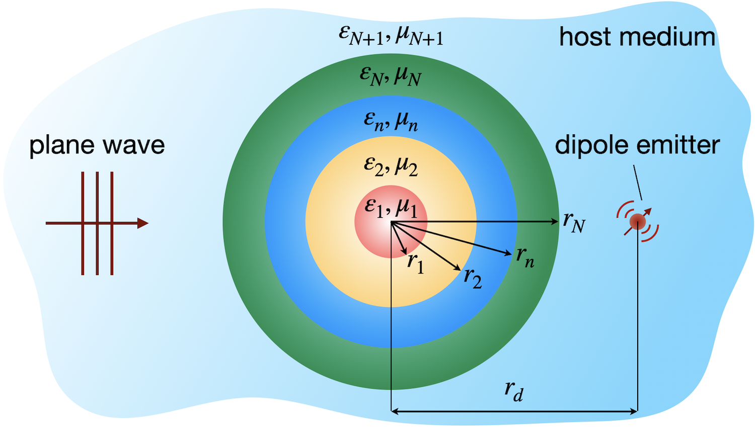
Figure 1: A sketch of the multilayered sphere in a homogeneous isotropic host medium with permittivity $\varepsilon_{h}=\varepsilon_{N+1}$ and permeability $\mu_{h}=\mu_{N+1}$. Center of the sphere is located at the origin of the reference system.

The sphere core counts as a shell with number $n=1$ and the host medium is the $n=N+1$ shell. Occasionally, the host medium will be denoted as $n=h$. Each shell has the outer radius $r_{n}$ and is assumed to be homogeneous and isotropic with scalar permittivity $\varepsilon_{n}$ and permeability $\mu_{n}$. Respective refractive indices are $\eta_{n}=\sqrt{\varepsilon_{n}\mu_{n}}$. We assume that the multilayered sphere is illuminated with a harmonic electromagnetic wave (either a plane wave or a dipole source) having vacuum wavelength $\lambda$. Corresponding wave vector in the $n$-th shell is $k_{n}=\eta_{n}\omega/c=2\pi\eta_{n}/\lambda$, where $c$ is the speed of light in vacuum, and $\omega$ is frequency. Electromagnetic fields in any shell are described by the stationary macroscopic Maxwell’s equations (with time dependence $e^{-i\omega t}$ assumed and suppressed throughout the paper):

$${\bf E}=\frac{ic}{\omega\varepsilon}\,\left(\mbox{\boldmath$\nabla$}\times{\bf H}\right)\ ,\qquad{\bf H}=-\frac{ic}{\omega\mu}\,\left(\mbox{\boldmath$\nabla$}\times{\bf E}\right)\ ,$$ (1)

where the permittivity $\varepsilon$ and permeability $\mu$ are scalars. Following the notation of [68], the basis of normalized (the normalization here refers to angular integration) transverse vector multipole fields $\mbox{\boldmath$\nabla$}\cdot{\bf F}_{pL}\equiv 0$ that satisfy the vector Helmholtz equation

$$\mbox{\boldmath$\nabla$}\times\left[\mbox{\boldmath$\nabla$}\times{\bf F}_{pL}(k,{\bf r})\right]=k^{2}{\bf F}_{pL}(k,{\bf r})$$ (2)

for $n$-th shell, $1\leq n\leq N+1$, can be formed as:

$$\begin{split}{\bf F}&{}_{ML}(k_{n},{\bf r})=f_{ML}(k_{n}r){\bf Y}^{(m)}_{L}({\bf r})\ ,\\ {\bf F}&{}_{EL}(k_{n},{\bf r})=\frac{1}{k_{n}r}\left\{\sqrt{\ell(\ell+1)}f_{EL}(k_{n}r){\bf Y}^{(o)}_{L}({\bf r})+\dfrac{\rm d}{{\rm d}r}\left[rf_{EL}(k_{n}r)\right]{\bf Y}^{(e)}_{L}({\bf r})\right\}\ ,\end{split}$$ (3)

where

$$\tilde{\bf F}_{EL}(k_{n},{\bf r})=\frac{1}{k_{n}}\mbox{\boldmath$\nabla$}\times{\bf F}_{ML}(k_{n},{\bf r})\ ,\quad\tilde{\bf F}_{ML}(k_{n},{\bf r})=\frac{1}{k_{n}}\mbox{\boldmath$\nabla$}\times{\bf F}_{EL}(k_{n},{\bf r})\ ,$$ (4)

with $\tilde{f}_{EL}=f_{ML}$ and $\tilde{f}_{ML}=f_{EL}$. Here $L=\ell,m$ is a composite angular momentum index and $f_{pL}$ is a suitable linear combination of spherical Bessel functions. Provided that the multipole fields in (3) represent ${\bf E}$, the respective subscripts $p=M$ and $p=E$ denote the magnetic, or transverse electric (TE), and electric, or transverse magnetic (TM), polarizations [88]. The so-called magnetic, ${\bf Y}^{(m)}_{L}$, longitudinal, ${\bf Y}^{(o)}_{L}$, and electric, ${\bf Y}^{(e)}_{L}$, vector spherical harmonics of degree $\ell$ and order $m$, are defined in spherical $(\varphi,\vartheta,r)$ coordinates as [89, 77, 88, 90]

$$\begin{split}{\bf Y}^{(m)}_{L}&=i\sqrt{\frac{(\ell-m)!}{(\ell+m)!}}\sqrt{\frac{2\ell+1}{4\pi\ell(\ell+1)}}\left[\hat{\bf e}_{\vartheta}\frac{imP_{\ell}^{m}(\cos\vartheta)}{\sin\vartheta}-\hat{\bf e}_{\varphi}\frac{{\rm d}P_{\ell}^{m}(\cos\vartheta)}{{\rm d}\vartheta}\right]\exp\left(im\varphi\right)\ ,\\ {\bf Y}^{(o)}_{L}&=i\sqrt{\frac{(\ell-m)!}{(\ell+m)!}}\sqrt{\frac{2\ell+1}{4\pi}}P_{\ell}^{m}(\cos\vartheta)\exp\left(im\varphi\right)\hat{\bf e}_{r}\ ,\\ {\bf Y}^{(e)}_{L}&=i\sqrt{\frac{(\ell-m)!}{(\ell+m)!}}\sqrt{\frac{2\ell+1}{4\pi\ell(\ell+1)}}\left[\hat{\bf e}_{\vartheta}\frac{{\rm d}P_{\ell}^{m}(\cos\vartheta)}{{\rm d}\vartheta}+\hat{\bf e}_{\varphi}\frac{imP_{\ell}^{m}(\cos\vartheta)}{\sin\vartheta}\right]\exp\left(im\varphi\right)\ ,\end{split}$$ (5)

where $\hat{\bf e}_{\varphi}$, $\hat{\bf e}_{\vartheta}$, and $\hat{\bf e}_{r}$ are corresponding unit vectors, and $P^{m}_{\ell}(x)$ are the associated Legendre functions of the first kind [91] of degree $\ell$ and order $m$:

$$P^{m}_{\ell}(x)=\frac{(-1)^{m}}{2^{\ell}\ell!}(1-x^{2})^{m/2}\frac{{\rm d}^{\ell+m}}{{\rm d}x^{\ell+m}}(x^{2}-1)^{\ell}\ .$$

General solution for the electric field in the $n$-th shell, $1\leq n\leq N+1$, is [68, Eq. (8)]:

$${\bf E}_{p}({\bf r})=\sum_{L}{\bf F}_{pL}(k_{n},{\bf r})=\sum_{L}\left[A_{pL}(n)\,{\bf J}_{pL}(k_{n},{\bf r})+B_{pL}(n)\,{\bf H}_{pL}(k_{n},{\bf r})\right]\ .$$ (6)

In order to emphasize and for the sake of tracking the Bessel function dependence, the multipoles ${\bf F}_{pL}$ in Eq. (6) are denoted as ${\bf J}_{pL}$ and ${\bf H}_{pL}$ for the respective cases that $f_{p\ell}=j_{\ell}$ and $f_{p\ell}=h_{\ell}^{(1)}$, where $j_{\ell}$ and $h_{\ell}^{(1)}$ being the spherical Bessel functions of the first and third kind, correspondingly.

Given the general solution (6), the corresponding expansion of magnetic field ${\bf H}$ follows from that of the electric field ${\bf E}$ by the stationary macroscopic Maxwell’s equations (1) on using relations (4) [68, Eqs. (9)-(10)]:

$$\begin{split}{\bf H}_{E}({\bf r})&=-i\dfrac{\varepsilon_{n}}{\mu_{n}}\sum_{L}\left[A_{EL}(n)\,{\bf J}_{ML}(k_{n},{\bf r})+B_{EL}(n)\,{\bf H}_{ML}(k_{n},{\bf r})\right]\ ,\\ {\bf H}_{M}({\bf r})&=-i\dfrac{\varepsilon_{n}}{\mu_{n}}\sum_{L}\left[A_{ML}(n)\,{\bf J}_{EL}(k_{n},{\bf r})+B_{ML}(n)\,{\bf H}_{EL}(k_{n},{\bf r})\right]\ .\end{split}$$ (7)

The ${\bf H}_{pL}$’s in Eqs. (6)-(7) with angular-momentum index $L$ refer to a basis multipole which distinguishes them from the magnetic field ${\bf H}_{p}$.

Very much as in the case of planar stratified media [79, 80, 81, 82], our RTMM for spherical interfaces exploits to the maximum the property that once the coefficients $A_{pL}(n+1)$ and $B_{pL}(n+1)$ on one side of a $n$-th shell interface are known, the coefficients $A_{pL}(n)$ and $B_{pL}(n)$ on the other side of the shell interface can be unambiguously determined, and vice versa. Schematically,

$$\begin{pmatrix}A_{pL}(n+1)\\ B_{pL}(n+1)\end{pmatrix}=T_{p\ell}^{+}(n)\begin{pmatrix}A_{pL}(n)\\ B_{pL}(n)\end{pmatrix}\ ,\qquad\begin{pmatrix}A_{pL}(n)\\ B_{pL}(n)\end{pmatrix}=T_{p\ell}^{-}(n)\begin{pmatrix}A_{pL}(n+1)\\ B_{pL}(n+1)\end{pmatrix}\ ,$$ (8)

where $T_{p\ell}^{\pm}(n)$ are $2\times 2$ transfer matrices [68]. The matrices, which are the fundamental quantities of our approach, can be viewed as a kind of raising and lowering ladder operators of quantum mechanics. In the present case, they lower and raise the argument $n$ of expansion coefficients $A_{pL}(n)$ and $B_{pL}(n)$. The transfer matrices are interrelated by

$$\left[T_{p\ell}^{+}(n)\right]^{-1}=T_{p\ell}^{-}(n)\ ,\qquad\left[T_{p\ell}^{-}(n)\right]^{-1}=T_{p\ell}^{+}(n)\ ,$$ (9)

and are unambiguously determined by matching fields across the $n$-th shell interface, i.e. requiring that the tangential components of ${\bf E}$ and ${\bf H}$ are continuous. One finds [68]:

$$T^{-}_{M\ell}(n)=-i\begin{pmatrix}\tilde{\eta}\zeta_{\ell}^{\prime}(x)\psi_{\ell}(\tilde{x})-\tilde{\mu}\zeta_{\ell}(x)\psi_{\ell}^{\prime}(\tilde{x})&\tilde{\eta}\zeta_{\ell}^{\prime}(x)\zeta_{\ell}(\tilde{x})-\tilde{\mu}\zeta_{\ell}(x)\zeta_{\ell}^{\prime}(\tilde{x})\\ -\tilde{\eta}\psi_{\ell}^{\prime}(x)\psi_{\ell}(\tilde{x})+\tilde{\mu}\psi_{\ell}(x)\psi_{\ell}^{\prime}(\tilde{x})&-\tilde{\eta}\psi_{\ell}^{\prime}(x)\zeta_{\ell}(\tilde{x})+\tilde{\mu}\psi_{\ell}(x)\zeta_{\ell}^{\prime}(\tilde{x})\end{pmatrix}\ ,$$ (10)

$$T^{-}_{E\ell}(n)=-i\begin{pmatrix}\tilde{\mu}\zeta_{\ell}^{\prime}(x)\psi_{\ell}(\tilde{x})-\tilde{\eta}\zeta_{\ell}(x)\psi_{\ell}^{\prime}(\tilde{x})&\tilde{\mu}\zeta_{\ell}^{\prime}(x)\zeta_{\ell}(\tilde{x})-\tilde{\eta}\zeta_{\ell}(x)\zeta_{\ell}^{\prime}(\tilde{x})\\ -\tilde{\mu}\psi_{\ell}^{\prime}(x)\psi_{\ell}(\tilde{x})+\tilde{\eta}\psi_{\ell}(x)\psi_{\ell}^{\prime}(\tilde{x})&-\tilde{\mu}\psi_{\ell}^{\prime}(x)\zeta_{\ell}(\tilde{x})+\tilde{\eta}\psi_{\ell}(x)\zeta_{\ell}^{\prime}(\tilde{x})\end{pmatrix}\ ,$$ (11)

$$T^{+}_{M\ell}(n)=-i\begin{pmatrix}\zeta_{\ell}^{\prime}(\tilde{x})\psi_{\ell}(x)/\tilde{\eta}-\zeta_{\ell}(\tilde{x})\psi_{\ell}^{\prime}(x)/\tilde{\mu}&\zeta_{\ell}^{\prime}(\tilde{x})\zeta_{\ell}(x)/\tilde{\eta}-\zeta_{\ell}(\tilde{x})\zeta_{\ell}^{\prime}(x)/\tilde{\mu}\\ -\psi_{\ell}^{\prime}(\tilde{x})\psi_{\ell}(x)/\tilde{\eta}+\psi_{\ell}(\tilde{x})\psi_{\ell}^{\prime}(x)/\tilde{\mu}&-\psi_{\ell}^{\prime}(\tilde{x})\zeta_{\ell}(x)/\tilde{\eta}+\psi_{\ell}(\tilde{x})\zeta_{\ell}^{\prime}(x)/\tilde{\mu}\end{pmatrix}\ ,$$ (12)

$$T^{+}_{E\ell}(n)=-i\begin{pmatrix}\zeta_{\ell}^{\prime}(\tilde{x})\psi_{\ell}(x)/\tilde{\mu}-\zeta_{\ell}(\tilde{x})\psi_{\ell}^{\prime}(x)/\tilde{\eta}&\zeta_{\ell}^{\prime}(\tilde{x})\zeta_{\ell}(x)/\tilde{\mu}-\zeta_{\ell}(\tilde{x})\zeta_{\ell}^{\prime}(x)/\tilde{\eta}\\ -\psi_{\ell}^{\prime}(\tilde{x})\psi_{\ell}(x)/\tilde{\mu}+\psi_{\ell}(\tilde{x})\psi_{\ell}^{\prime}(x)/\tilde{\eta}&-\psi_{\ell}^{\prime}(\tilde{x})\zeta_{\ell}(x)/\tilde{\mu}+\psi_{\ell}(\tilde{x})\zeta_{\ell}^{\prime}(x)/\tilde{\eta}\end{pmatrix}\ ,$$ (13)

where $\psi_{\ell}(x)=xj_{\ell}(x)$ and $\zeta_{\ell}(x)=xh^{(1)}_{\ell}(x)$ are the Riccati-Bessel functions, prime denotes the derivative with respect to the argument in parentheses, $x_{n}=k_{n}r_{n}$ and $\tilde{x}_{n}=x_{n}/\tilde{\eta}_{n}=k_{n+1}r_{n}$ are the internal and external dimensionless size parameters, $\tilde{\eta}_{n}=\eta_{n}/\eta_{n+1}$ and $\tilde{\mu}_{n}=\mu_{n}/\mu_{n+1}$ are relative refractive indices and permeabilities. For the sake of clarity, the $n$-subscript has been suppressed on the rhs of Eqs. (10) – (13). The above expressions for $T^{\pm}_{p\ell}(n)$ are general, independent on the incident field, and valid for any homogeneous and isotropic medium, including gain ($\Im(\varepsilon_{n})<0$) or magnetic materials ($\mu_{n}\neq 1$).

The formalism becomes compact upon the use of the composite transfer matrices ${\cal T}_{p\ell}(n)$ and ${\cal M}_{p\ell}(n)$ defined as ordered (from the left to the right) products of the constituent raising and lowering $2\times 2$ matrices from Eqs. (10)-(13):

$${\cal T}_{p\ell}(n)=\prod_{j=n-1}^{1}T_{p\ell}^{+}(j)\ ,\qquad{\cal M}_{p\ell}(n)=\prod_{j=n}^{N}T_{p\ell}^{-}(j)\ .$$ (14)

Composite matrices ${\cal T}_{p\ell}(n)$ and ${\cal M}_{p\ell}(n)$ transfer expansion coefficients to the $n$-th shell from the sphere core or from the surrounding medium, respectively. Note that ${\cal T}_{p\ell}(n)$ are defined for $2\leq n\leq N+1$, while ${\cal M}_{p\ell}(n)$ are defined for $1\leq n\leq N$. They are used in our formalism to chiefly relate the expansion coefficients in the core to those in a source region. For example, ${\cal T}_{p\ell}(N+1)$ enables one to obviate all the intermediary shell interfaces and to relate the expansion coefficients in the core directly to those in the surrounding host medium,

$$\begin{pmatrix}A_{pL}(N+1)\\ B_{pL}(N+1)\end{pmatrix}={\cal T}_{p\ell}(N+1)\begin{pmatrix}A_{pL}(1)\\ B_{pL}(1)\end{pmatrix}\ .$$ (15)

The latter formally reduces the problem of a multilayered sphere with a source in the host medium to that of a homogeneous sphere. Analogously to (9):

$$\left[{\cal T}_{p\ell}(N+1)\right]^{-1}={\cal M}_{p\ell}(1)\ ,\qquad\left[{\cal M}_{p\ell}(1)\right]^{-1}={\cal T}_{p\ell}(N+1)\ .$$ (16)

The reader familiar with the RTMM for planar stratified media (e.g. multilayer coatings and interference filters) will recognize in the relations (8), (9), (14), (15), (16) familiar properties of the constituent and composite transfer matrices for planar interfaces [79, 80, 81, 82].

In order to unambiguously determine the expansion coefficients $A_{pL}(n)$ and $B_{pL}(n)$ in each shell, one has to impose two boundary conditions, which is the subject of the following section.

2.2 Boundary conditions

The total number of different sets of expansion coefficients comprising all $j$’s from the interval $1\leq j\leq N+1$ is larger by two than the number of corresponding equations. Therefore, boundary conditions have to be imposed to unambiguously determine the expansion coefficients at any shell. They are

1. The regularity condition of the solution at the sphere origin, which eliminates $h_{\ell}^{(1)}(0)\to\infty$ for $f_{p\ell}$ in Eq. (3):

   $$B_{EL}(1)=B_{ML}(1)\equiv 0\ .$$ (17)

2. For a source located outside a sphere, the $A_{pL}(N+1)$ coefficients at any given frequency $\omega$ are equal to the expansion coefficients of an incident electromagnetic field in spherical coordinates.

The regularity condition (17) alone suffices to unambiguously determine the $m$-independent (due to spherical symmetry of a problem) ratio [88]:

$${\cal T}_{21;p\ell}(N+1)/{\cal T}_{11;p\ell}(N+1)=\mathbb{T}_{p\ell},$$ (18)

which defines the familiar T-matrix of scattering theory, $\mathbb{T}_{p\ell}$, where $i,j$ in ${\cal T}_{ij;p\ell}(n)$ label the $(i,j)$-th element of the $2\times 2$ matrix ${\cal T}_{p\ell}(n)$. Note that $\mathbb{T}_{p\ell}$ are nothing but familiar expansion coefficients $a_{\ell}$ and $b_{\ell}$ in Bohren and Huffman’s representation [77, Eqs. (4.56),(4.57)], but with the opposite sign: $\mathbb{T}_{E\ell}=-a_{\ell}$ and $\mathbb{T}_{M\ell}=-b_{\ell}$.

Corresponding closed-form analytic expressions for applying the second boundary condition are presented in (i) Refs. [90],[70, Eq. (10)] for the plane electromagnetic wave, and in (ii) Ref. [68, Eqs. (44),(50)] for the electric dipole source. In the case of an elementary dipole radiating inside a sphere, there is no source outside a sphere, and the second boundary condition reduces to $A_{pL}(N+1)=0$ [68].

2.3 Far-field properties

Fundamental cross sections $\sigma$ (scattering, absorption and extinction) are determined as an infinite sum over polarizations ($p=E,M$) and all partial $\ell$-waves:

$$\begin{split}\sigma_{\rm sca}=\sum_{p,\ell}\sigma_{{\rm sca};p\ell}&=\dfrac{\pi}{k_{h}^{2}}\sum_{p,\ell}\left(2\ell+1\right)\left|\mathbb{T}_{p\ell}\right|^{2}\ ,\\ \sigma_{\rm abs}=\sum_{p,\ell}\sigma_{{\rm abs};p\ell}&=\dfrac{\pi}{2k_{h}^{2}}\sum_{p,\ell}\left(2\ell+1\right)\left(1-\left|1+2\mathbb{T}_{p\ell}\right|^{2}\right)\ ,\\ \sigma_{\rm ext}=\sum_{p,\ell}\sigma_{{\rm ext};p\ell}&=-\dfrac{2\pi}{k_{h}^{2}}\sum_{p,\ell}\left(2\ell+1\right)\Re\left(\mathbb{T}_{p\ell}\right)\ ,\end{split}$$ (19)

where $\Re$ takes the real part, and $\mathbb{T}_{p\ell}$ is found from Eq. (18).

On using polarized scattering waves parallel and perpendicular to the scattering plane,

$$\begin{split}S_{\parallel}(\vartheta)&=-\sum_{\ell}\dfrac{2\ell+1}{\ell(\ell+1)}\left[\mathbb{T}_{E\ell}\frac{{\rm d}P_{\ell}^{1}(\cos\vartheta)}{{\rm d}\vartheta}+\mathbb{T}_{M\ell}\frac{P_{\ell}^{1}(\cos\vartheta)}{\sin\vartheta}\right]\ ,\\ S_{\perp}(\vartheta)&=-\sum_{\ell}\dfrac{2\ell+1}{\ell(\ell+1)}\left[\mathbb{T}_{M\ell}\frac{{\rm d}P_{\ell}^{1}(\cos\vartheta)}{{\rm d}\vartheta}+\mathbb{T}_{E\ell}\frac{P_{\ell}^{1}(\cos\vartheta)}{\sin\vartheta}\right]\ ,\end{split}$$ (20)

one can easily build up scattering matrix, find Stokes parameters [77, Eq. (4.77)], and obtain angle-resolved scattering pattern.

2.4 Near-field properties

For a given illumination, and, thus, known expansion coefficients $A_{pL}(n)$ and $B_{pL}(n)$, the electromagnetic field can be unambiguously defined by Eqs. (6) and (7). Below we consider more sophisticated near-field properties.

2.4.1 Electromagnetic energy

Total electromagnetic energy $W$ stored within a multilayered sphere is a sum of energies, $W_{n}$, stored within any given $n$-th shell, which in turn is an integral of an electromagnetic energy density $w_{n}(r)$ over the $n$-th shell:

$$W=\sum_{n=1}^{N}W_{n}=\sum_{n=1}^{N}\int_{r_{n-1}}^{r_{n}}w_{n}(r)r^{2}{\rm d}r\ ,\quad w_{n}(r)=\dfrac{1}{4}\oint\left[G_{e}(\varepsilon_{n})\left|{\bf E}({\bf r})\right|^{2}+G_{m}(\mu_{n})\left|{\bf H}({\bf r})\right|^{2}\right]{\rm d}\Omega\ ,$$ (21)

where $r_{0}=0$, i.e. the core “inner radius”. Here we limit the discussion to a plane wave excitation. For non-dispersive (usually dielectric) shells [92], electric and magnetic coefficients in (21) are

$$G_{e}(\varepsilon_{n})=\Re(\varepsilon_{n})\ ,\qquad G_{m}(\mu_{n})=\Re(\mu_{n})\ ,$$ (22)

while for the dispersive and absorbing shells [93]:

$$G_{e}(\varepsilon_{n},\omega)=\Re(\varepsilon_{n})+\dfrac{2\omega}{\gamma_{D}}\Im(\varepsilon_{n})\ ,$$ (23)

where $\gamma_{D}$ is the free electron damping constant in the Drude formula, and $\Im$ takes the imaginary part. In our code, we use Drude fit parameters from either Blaber et al. [94] or Ordal et al. [95].

Electric and magnetic components from Eq. (21) are nothing but the orientation-averaged electric and magnetic field intensities:

$$\begin{split}\oint\left|{\bf E}\right|^{2}\,{\rm d}\Omega&=2\pi|E_{0}|^{2}\sum_{\ell=1}^{\infty}\left[(2\ell+1)\,|\bar{f}_{M\ell}|^{2}+(\ell+1)\,|\bar{f}_{E,\ell-1}|^{2}+\ell\,|\bar{f}_{E,\ell+1}|^{2}\right]\ ,\\ \oint\left|{\bf H}\right|^{2}\,{\rm d}\Omega&=2\pi|E_{0}|^{2}\frac{|\varepsilon_{n}|}{|\mu_{n}|}\sum_{\ell=1}^{\infty}\left[(2\ell+1)\,|\bar{f}_{E\ell}|^{2}+(\ell+1)\,|\bar{f}_{M,\ell-1}|^{2}+\ell\,|\bar{f}_{M,\ell+1}|^{2}\right]\ .\end{split}$$ (24)

Here $\bar{f}_{p\ell,\ell\pm 1}=\bar{A}_{p\ell}(n)j_{\ell,\ell\pm 1}(k_{n}r)+\bar{B}_{p\ell}(n)h^{(1)}_{\ell,\ell\pm 1}(k_{n}r)$. Note that in all cases the spherical Bessel functions of either $\ell$ and $\ell\pm 1$ orders are multiplied by the expansions coefficients $\bar{A}_{p\ell}$ and $\bar{B}_{p\ell}$ with the index $\ell$. These expansion coefficients are determined via raising ${\cal T}_{p\ell}(n)$ and lowering ${\cal M}_{p\ell}(n)$ composite transfer matrices as

$$\bar{A}_{p\ell}(n)=\begin{cases}1/{\cal T}_{11;p\ell}(N+1)\ ,&n=1\ ,\\ {\cal M}_{11;p\ell}(n)+{\cal M}_{12;p\ell}(n)\dfrac{{\cal T}_{21;p\ell}(N+1)}{{\cal T}_{11;p\ell}(N+1)}\ ,&1<n<N+1\ ,\\ 1\ ,&n=N+1\ ,\end{cases}$$ (25)

$$\bar{B}_{p\ell}(n)=\begin{cases}0\ ,&n=1\ ,\\ {\cal M}_{21;p\ell}(n)+{\cal M}_{22;p\ell}(n)\dfrac{{\cal T}_{21;p\ell}(N+1)}{{\cal T}_{11;p\ell}(N+1)}\ ,&1<n<N+1\ ,\\ \dfrac{{\cal T}_{21;p\ell}(N+1)}{{\cal T}_{11;p\ell}(N+1)}\ ,&n=N+1\ .\end{cases}$$ (26)

Because the surface integrals of electric and magnetic field intensities are performed analytically [70], the calculation of average intensity costs the same computational time as determining intensity at a single given point.

The radial integrations in (21) are performed by using Lommel’s integration formulas [70]:

$$\begin{split}\int_{r_{n-1}}^{r_{n}}r^{2}{\rm d}r&\oint\left|{\bf E}\right|^{2}{\rm d}\Omega=\\ &2\pi|E_{0}|^{2}\frac{r^{3}}{x^{2}-x^{*2}}\left.\sum_{\ell=1}^{\infty}\left[(2\ell+1)\bar{F}_{M\ell}+(\ell+1)\bar{F}_{E,\ell-1}+\ell\bar{F}_{E,\ell+1}\right]\right|_{r=r_{n-1}}^{r=r_{n}}\ ,\\ \int_{r_{n-1}}^{r_{n}}r^{2}{\rm d}r&\oint\left|{\bf H}\right|^{2}{\rm d}\Omega=\\ &2\pi|E_{0}|^{2}\frac{r^{3}}{x^{2}-x^{*2}}\frac{|\varepsilon_{n}|}{|\mu_{n}|}\left.\sum_{\ell=1}^{\infty}\left[(2\ell+1)\bar{F}_{E\ell}+(\ell+1)\bar{F}_{M,\ell-1}+\ell\bar{F}_{M,\ell+1}\right]\right|_{r=r_{n-1}}^{r=r_{n}}\ .\end{split}$$ (27)

Here $x=k_{n}r$, and purely imaginary functions $\bar{F}_{p\ell}=2i\Im\left(x\bar{f}_{p\ell+1}(x)\bar{f}^{*}_{p\ell}(x)\right)$ are cancelled by purely imaginary $x^{2}-x^{*2}=4i\Re(x)\Im(x)$ in the denominator, which results in purely real integrals in (27). For a special case of lossless shells, the denominator $x^{2}-x^{*2}$ vanishes. It can be eliminated by using l’Hôpital’s rule [70] to get the following amendments in Eq. (27): $x^{2}-x^{*2}\to 2x$ and $\bar{F}_{p\ell}\ \to x\left(|\bar{f}_{p\ell}(x)|^{2}+|\bar{f}_{p\ell+1}(x)|^{2}\right)-(2\ell+1)\Re\left(\bar{f}_{p\ell}(x)\bar{f}^{*}_{p\ell+1}(x)\right)$.

Substitution of (24) and (27) into (21) yields in explicit expressions for the total electromagnetic energy $W_{n}$ stored within each shell of the multilayered sphere and for the electromagnetic energy density $w_{n}(r)$. These relations are general and valid for any shell, including the $(N+1)$-th shell being a surrounding medium. For the comprehensive derivation of the equations above, we refer the Reader to the Ref. [70], which generalizes the pioneering work by Bott and Zdunkowski on homogeneous spheres [92] and subsequent follow-ups for magnetic spheres [96] and core-shells [97].

2.4.2 Spontaneous decay rates

Radiative and nonradiative decay rates (normalized with respect to $\Gamma_{\rm rad;0}$, the intrinsic radiative decay rate in the absence of a multilayered sphere) for a dipole emitter located in $n_{d}$-th shell at $r_{d}$ distance from a center of a sphere (see Fig. 1) are given by [68]:

$$\begin{split}\dfrac{\Gamma^{\perp}_{\rm rad}}{\Gamma_{\rm rad;0}}&=\dfrac{3}{2x_{d}^{4}}{\cal N}_{\rm rad}\sum_{\ell=1}^{\infty}\ell(\ell+1)(2\ell+1)\left|{\cal F}_{E\ell}(x_{d})\right|^{2}\ ,\\ \dfrac{\Gamma^{\parallel}_{\rm rad}}{\Gamma_{\rm rad;0}}&=\dfrac{3}{4x_{d}^{2}}{\cal N}_{\rm rad}\sum_{\ell=1}^{\infty}(2\ell+1)\left[\left|{\cal F}_{M\ell}(x_{d})\right|^{2}+\left|{\cal F}^{\;\prime}_{E\ell}(x_{d})\right|^{2}\right]\ ,\\ \dfrac{\Gamma^{\perp}_{\rm nrad}}{\Gamma_{\rm rad;0}}&=\dfrac{3k^{3}_{d}}{2x_{d}^{4}}{\cal N}_{\rm nrad}\sum_{\Im(\varepsilon_{a})>0}\Im(\varepsilon_{a})\sum_{\ell=1}^{\infty}\ell(\ell+1)(2\ell+1)I_{E\ell;a}\left|{\cal D}_{E\ell;a}(x_{d})\right|^{2}\ ,\\ \dfrac{\Gamma^{\parallel}_{\rm nrad}}{\Gamma_{\rm rad;0}}&=\dfrac{3k^{3}_{d}}{4x_{d}^{2}}{\cal N}_{\rm nrad}\sum_{\Im(\varepsilon_{a})>0}\Im(\varepsilon_{a})\sum_{\ell=1}^{\infty}(2\ell+1)\left[I_{M\ell;a}\left|{\cal D}_{M\ell;a}(x_{d})\right|^{2}+I_{E\ell;a}\left|{\cal D}^{\prime}_{E\ell;a}(x_{d})\right|^{2}\right]\ ,\end{split}$$ (28)

where $x_{d}=k_{d}r_{d}$ and $k_{d}=2\pi\eta_{d}/\lambda$. Coefficients ${\cal N}_{\rm rad}$ and ${\cal N}_{\rm nrad}$ depend on whether the decay rates were normalized with respect to the radiative decay rates in infinite homogeneous medium having the refractive index of (i) the host or (ii) having the refractive index of the shell where the dipole emitter is located:

$${\cal N}^{\rm host}_{\rm rad}=\dfrac{\eta_{d}^{3}}{\varepsilon_{d}}\dfrac{\varepsilon_{h}}{\eta^{3}_{h}}\ ,\quad{\cal N}^{\rm shell}_{\rm rad}=\left(\dfrac{\eta_{d}}{\eta_{h}}\right)^{6}\left(\dfrac{\varepsilon_{h}}{\varepsilon_{d}}\right)^{2}\ ,\qquad{\cal N}^{\rm host}_{\rm nrad}=\dfrac{\eta_{d}^{3}}{\eta^{3}_{h}}\dfrac{\varepsilon_{h}}{\varepsilon_{d}^{2}}\ ,\quad{\cal N}^{\rm shell}_{\rm nrad}=\dfrac{1}{\varepsilon_{d}}\cdot$$ (29)

Functions ${\cal F}_{p\ell}(x_{d})$ and ${\cal D}_{p\ell;a}(x_{d})$ depend on the relative position of the emitter with respect to the sphere, and to a $n_{a}$-th absorbing shell:

$${\cal F}_{p\ell}(x_{d})=\begin{cases}\dfrac{\psi_{\ell}(x_{d})}{{\cal M}_{21;p\ell}(1)}\ ,&n_{d}=1\ ,\\[10.0pt] \dfrac{{\cal T}_{11;p\ell}(n_{d})\psi_{\ell}(x_{d})+{\cal T}_{21;p\ell}(n_{d})\zeta_{\ell}(x_{d})}{{\cal T}_{11;p\ell}(n_{d}){\cal M}_{22;p\ell}(n_{d})-{\cal T}_{21;p\ell}(n_{d}){\cal M}_{12;p\ell}(n_{d})}\ ,&1<n_{d}\leq N\ ,\\[10.0pt] \psi_{\ell}(x_{d})+\dfrac{{\cal T}_{21;p\ell}(N+1)}{{\cal T}_{11;p\ell}(N+1)}\zeta_{\ell}(x_{d})\ ,&n_{d}=N+1\ ,\end{cases}$$ (30)

$${\cal D}_{p\ell;a}(x_{d})=\begin{cases}\dfrac{\psi_{\ell}(x_{d})}{{\cal M}_{21;p\ell}(1)}\ ,&n_{d}=1\ ,\\[10.0pt] \dfrac{{\cal T}_{11;p\ell}(n_{d})\psi_{\ell}(x_{d})+{\cal T}_{21;p\ell}(n_{d})\zeta_{\ell}(x_{d})}{{\cal T}_{11;p\ell}(n_{d}){\cal M}_{22;p\ell}(n_{d})-{\cal T}_{21;p\ell}(n_{d}){\cal M}_{12;p\ell}(n_{d})}\ ,&1<n_{d}<n_{a}\ ,\\[10.0pt] \dfrac{{\cal M}_{22;p\ell}(n_{d})\psi_{\ell}(x_{d})+{\cal M}_{12;p\ell}(n_{d})\zeta_{\ell}(x_{d})}{{\cal T}_{11;p\ell}(n_{d}){\cal M}_{22;p\ell}(n_{d})-{\cal T}_{21;p\ell}(n_{d}){\cal M}_{12;p\ell}(n_{d})}\ ,&n_{a}<n_{d}\leq N\ ,\\[10.0pt] \zeta_{\ell}\left(x_{d}\right)\ ,&n_{d}=N+1\ .\end{cases}$$ (31)

The summation over nonradiative decay channels in Eqs. (28) includes each absorbing shell, i.e. shell with $\Im(\varepsilon_{a})>0$. Respective volume integrals $I_{E\ell;a}$ and $I_{M\ell;a}$ are

$$\begin{split}I_{M\ell;a}=&\dfrac{1}{|k_{a}|^{2}}\int_{a}\left|{\cal A}_{M\ell;a}\psi_{\ell}(k_{a}r)+{\cal B}_{M\ell;a}\zeta_{\ell}(k_{a}r)\right|^{2}{\rm d}r\ ,\\ I_{E\ell;a}=&\dfrac{\ell(\ell+1)}{|k_{a}|^{4}}\int_{a}\left|{\cal A}_{E\ell;a}\psi_{\ell}(k_{a}r)+{\cal B}_{E\ell;a}\zeta_{\ell}(k_{a}r)\right|^{2}\dfrac{{\rm d}r}{r^{2}}+\\ &\dfrac{1}{|k_{a}|^{2}}\int_{a}\left|{\cal A}_{E\ell;a}\psi^{\prime}_{\ell}(k_{a}r)+{\cal B}_{E\ell;a}\zeta^{\prime}_{\ell}(k_{a}r)\right|^{2}{\rm d}r\ .\end{split}$$ (32)

Here $k_{a}=2\pi\eta_{a}/\lambda$ is the wavevector in the absorbing shell, and coefficients ${\cal A}_{p\ell;a}$ and ${\cal B}_{p\ell;a}$ are

$${\cal A}_{p\ell;a}=\begin{cases}1\ ,&n_{a}=1\;\text{and}\;n_{d}<N+1\ ,\\[10.0pt] {\cal T}_{11;p\ell}(n_{a})\ ,&1<n_{a}<n_{d}<N+1\ ,\\[10.0pt] {\cal M}_{12;p\ell}(n_{a})\ ,&n_{d}<n_{a}\ ,\\[10.0pt] {\cal M}_{11;p\ell}(n_{a})+{\cal M}_{12;p\ell}(n_{a})\dfrac{{\cal T}_{21;p\ell}(N+1)}{{\cal T}_{11;p\ell}(N+1)}\ ,&n_{d}=N+1\ ,\end{cases}$$ (33)

$${\cal B}_{p\ell;a}=\begin{cases}0\ ,&n_{a}=1\ ,\\[10.0pt] {\cal T}_{21;p\ell}(n_{a})\ ,&1<n_{a}<n_{d}<N+1\ ,\\[10.0pt] {\cal M}_{22;p\ell}(n_{a})\ ,&n_{d}<n_{a}\ ,\\[10.0pt] {\cal M}_{21;p\ell}(n_{a})+{\cal M}_{22;p\ell}(n_{a})\dfrac{{\cal T}_{21;p\ell}(N+1)}{{\cal T}_{11;p\ell}(N+1)}\ ,&n_{a}\neq 1\;\text{and}\;n_{d}=N+1\ .\end{cases}$$ (34)

Note that ${\cal A}_{p\ell;a}$ and ${\cal B}_{p\ell;a}$ depend only on the relative position of the dipole with respect to the absorbing shell. We make use of this property to optimize calculations, namely, we get $I_{E\ell;a}$ and $I_{M\ell;a}$ once for a set of $r_{d}$, considering only the relative position of the dipole emitter.

For the detailed discussion of the spontaneous decay rates of a dipole emitter in a presence of a general multilayered sphere, we refer the reader to Ref. [68].

2.5 Convergence criteria

Numerical implementation of equations above, which involve infinite summation over $\ell$, requires truncation at some finite number $\ell_{\rm max}$. For far-field properties, Eqs. (19) and (20), the classic choice is the Wiscombe criterion [98]:

$$\ell_{\rm max}=\begin{cases}x_{N}+4x_{N}^{1/3}+1\ ,\qquad 0.02\leq x_{N}\leq 8\ ,\\ x_{N}+4.05x_{N}^{1/3}+2\ ,\qquad 8<x_{N}\ ,\end{cases}$$ (35)

where $x_{N}=k_{h}r_{N}$ is the usual size parameter. Keeping in mind plasmonics and nanophotonics applications as intended for our package, and recalling finite precision of the MATLAB, we limit the discussion for multilayered spheres with $x_{N}<50$ requiring $\ell_{\rm max}\lesssim 70$, which is more than sufficient.

For the near-field, Eqs. (6), (7), and for the electromagnetic energy, Eqs. (21), (24), (27), slightly different cut-off is recommended [99]:

$$\ell_{\rm max}=x_{N}+11x_{N}^{1/3}+1\ .$$ (36)

For the dipole source implied in Eq. (28), especially when considering non-radiative decay rates [68, 100], the accuracy has to be set instead of $\ell_{\rm max}$, since there are no general guidelines for choosing the latter in this case.

2.6 Electron free path correction

For thin metallic shell with thickness $(r_{n}-r_{n-1})$ less than a free electron path, the bulk permittivity $\varepsilon_{n,{\rm bulk}}$ has to be corrected to take into account electron scattering from the shell surface [101]:

$$\varepsilon_{n}\to\varepsilon_{n,{\rm bulk}}+\dfrac{\omega^{2}_{p}}{\omega^{2}+i\gamma_{D}\omega}-\dfrac{\omega^{2}_{p}}{\omega^{2}+i\gamma\omega}\ ,\quad\gamma=\gamma_{D}+\dfrac{\upsilon_{F}}{L_{\rm eff}}\ ,\quad L_{\rm eff}=\dfrac{4}{3}\dfrac{r_{n}^{3}-r_{n-1}^{3}}{r_{n}^{2}+r_{n-1}^{2}}\ ,$$ (37)

where $\upsilon_{F}$ is the Fermi velocity and $\omega_{p}$ is plasma frequency. This modification of thin metallic shells permittivity may have crucial consequences for their electromagnetic properties [102, 103, 20, 21, 104].

3 Computer code

3.1 Overview

Fundamental properties are calculated with the following functions:

• t_mat.m calculates transfer matrices with Eqs. (10) – (13) and returns their ordered products (14). Any other function which returns electromagnetic properties (decay rates, electromagnetic energy and fields, far-field properties and etc) makes use of pre-calculated ordered products of transfer matrices for a better performance;

• decay.m returns decay rates calculated with Eqs. (28). Decay rates are normalized (see Eqs. (29)) with respect to radiative decay rates of a dipole in a homogeneous medium (without a multilayered sphere) with the refractive index of a shell where the dipole is embedded, $\eta_{d}$, or with the refractive index of a host, $\eta_{h}$;

• nrg_dens.m returns normalized by the factor $\pi|E_{0}|^{2}\varepsilon_{h}$ [70, Sec.3E] electric and magnetic components of electromagnetic energy density, $w_{n}(r)$, given by Eq. (21), and orientation-averaged intensities of electric and magnetic fields given by Eq. (24);

• nrg_tot.m returns normalized by the factor $(2/3)\pi|E_{0}|^{2}(r_{n}-r_{n-1}^{3})\varepsilon_{h}$ [70, Sec.3E] electric and magnetic components of total electromagnetic energy $W_{n}$ stored within $n$-th shell given by Eq. (21);

• near_fld.m returns electric, ${\bf E}({\bf r})={\bf E}_{E}({\bf r})+{\bf E}_{M}({\bf r})$, and magnetic, ${\bf H}({\bf r})={\bf H}_{E}({\bf r})+{\bf H}_{M}({\bf r})$ near-field distributions given by Eqs. (6) and (7). We take the advantage of the spherical symmetry of the problem and pre-calculate computationally expensive ${\bf r}$-dependent Bessel functions and $\cos\theta$-dependent associated Legendre polynomials only for unique values of ${\bf r}$ and $\cos\theta$. Usually, the amount of these unique ${\bf r}$ and $\cos\theta$ is significantly smaller than the respective total number of points in the rectangular mesh, which results in faster execution;

• far_fld.m returns polarized scattering waves from Eq. (20);

• crs_sec.m returns fundamental cross sections from Eq. (19);

• el_fr_pth.m returns corrected permittivity according to Eq. (37).

Suitable combinations or minor post-processing of these fundamental characteristics may be used for almost every known application of multilayered spheres briefly discussed in Sec. 4 below.

3.2 Verification and performance

We have compared STRATIFY with freely available exact BEM-based [83] solver MNPBEM [84, 85, 86, 87]. The latter package has been chosen for a benchmark since it is a freely available comprehensive MATLAB code capable of calculating most of the quantities considered in our code. For testing purposes, we have considered fundamental cross-sections, electric near-field distribution, and spontaneous decay rates of dipole emitter in the presence of matryoshkas composed of different combinations of Au and SiO₂ layers. It can be easily seen from Fig. 2 that our code produces the same results as the exact BEM method, but for sufficiently lower computational price.

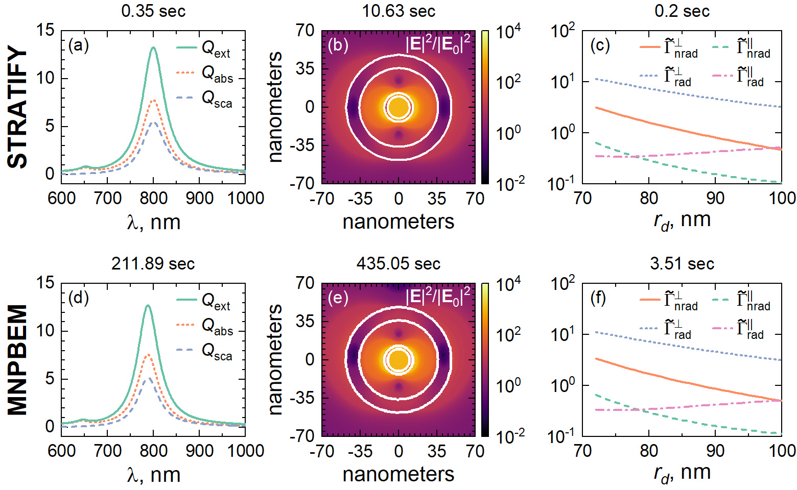
Figure 2: Comparison between our code (top, STRATIFY) and freely available BEM-based package (bottom, MNPBEM). (a),(d) Normalized fundamental cross-section ($Q=\sigma/\pi r_{2}^{2}$) of SiO₂@Au core-shell sphere with $\{r_{1},r_{2}\}=\{50,55\}$nm, in air host; (b),(e) intensity of the electric field for SiO₂@Au@SiO₂@Au matryoshka with $\{r_{1},r_{2},r_{3},r_{4}\}=\{10,13,36,48\}$ nm, in water host, at $\lambda=690$ nm [105, cf. Fig.3b]; (c),(f) normalized spontaneous decay rates ($\tilde{\Gamma}=\Gamma/\Gamma_{\rm rad;0}$) for the dipole emitter located at $r_{d}$ distance from the center of Au@SiO₂ core-shell sphere with $\{r_{1},r_{2}\}=\{50,70\}$ nm, in water host, at $\lambda=614$ nm. Run times of codes on a laptop with 2.6 GHz 6-Core Intel Core i7 processor are shown on top of each plot. For a fair comparison, the same number of points for $\lambda$ (801) in (a),(c), same $700\times 700$ mesh in (b),(e), and same number of points for $r_{d}$ (29) in (c),(f) are used. Note typically more than $50$ times faster speed of our package compared to the freely available BEM-based package.

4 Discussion and Conclusions

The developed package is ready to be applied in a number of well-established applications of multilayered spheres in optics and photonics. Below we discuss the most common examples. Due to enormous electric field enhancement in multilayered metal-dielectric nanospheres, they are considered as good candidates for a number of applications. Squared electric field intensities from Eq. (24) or Eq. (27) are measure for performance of nanostructures in SERS [25, 106, 107, 41, 108, 42] and second harmonic generation [8, 9]. For fluorescence or upconversion enhancement, where the spontaneous decay rates of the dipole emitters are modified, the generic enhancement factor is nothing but a product of excitation rate enhancement (at excitation wavelength, $\lambda_{\rm exc}$) and quantum yield (at emission wavelength, $\lambda_{\rm ems}$):

$$F=\dfrac{\gamma_{\rm exc}}{\gamma_{\rm exc;0}}\dfrac{q_{\rm ems}}{q_{\rm ems;0}}\ ,\qquad q_{\rm ems}=\dfrac{\Gamma_{\rm rad}/\Gamma_{{\rm rad};0}}{\Gamma_{\rm rad}/\Gamma_{{\rm rad};0}+\Gamma_{\rm nrad}/\Gamma_{{\rm rad};0}+(1-q_{\rm ems;0})/q_{\rm ems;0}}\cdot$$ (38)

Here $\gamma_{\rm exc}/\gamma_{\rm exc;0}\propto|{\bf E}|^{2\mathcal{P}}/|{\bf E}_{0}|^{2\mathcal{P}}$, $\mathcal{P}$ is the number of photons involved in the excitation process ($\mathcal{P}=1$ for fluorescence enhancement, $\mathcal{P}=2$ for the upconversion), $q_{\rm ems;0}$ is the intrinsic quantum yield of the emitter, and $\Gamma_{\rm rad,nrad}=(2\Gamma^{\parallel}_{\rm rad,nrad}+\Gamma^{\perp}_{\rm rad,nrad})/3$ is an orientationally averaged decay rate determined at a fixed dipole radial position by averaging over all possible orientations of a dipole emitter. Orientationnaly averaged fields in $\gamma_{\rm exc}$, and orientationally averaged decay rates, $\Gamma_{\rm rad,nrad}$, are reasonable choice for reliable estimates, unless, of course, the emitter is positioned with a controllable orientation of its electric dipole moment at a particular (e.g. a hot spot) location.

Cloaking, Kerker effect [109], super- or optimally tuned scattering [110, 111, 112, 113, 51, 114, 115] and absorption [116, 113, 117, 118, 20, 51, 115], embedded photonic eigenvalues [119], spasing [120, 44, 47, 121] and other intriguing phenomena [122] are easily understood from fundamental cross sections (19) and scattering patterns (20).

We have summarized a self-consistent and comprehensive RTMM theory reported earlier in our [68, 70] for electromagnetic light scattering from general multilayered spheres composed of isotropic shells. Within the framework of RTMM, we have developed an efficient multi-purpose MATLAB package for calculating fundamental properties of multilayered spheres. Our package is one-of-a-kind freely available software which allows for a simultaneous calculation of a wide range of electromagnetic properties and is ready to be used for a broad number of applications in chemistry, optics and photonics, including optimization problems and machine-learning studies. We hope that the generalization presented here and corresponding MATLAB code will serve as a useful tool for photonics, physics, chemistry and other scientific communities and will boost the researches involving various kinds of multilayered spheres.

Extensions of our code for ultra-thin metallic shell characterized by nonlocal dielectric functions [123, 124, 125, 126, 127, 128, 129, 130, 131, 132], an optically active shells [133, 134, 135, 136, 137, 138, 139, 140], or including perfectly conducting boundary conditions at the sphere core are, following the theory developed in Ref. [68], rather straightforward. Further generalization of the package may include illumination with focused, Gaussian, or other beams [141, 66, 64, 142]. An incorporation of magnetic dipole emitters [143, 144, 145] or modeling the effect of a multilayered sphere on the far-field radiation directivity of a dipole antenna should follow soon.

References

- [1] A. E. Neeves and M. H. Birnboim, “Composite structures for the enhancement of nonlinear optical materials,” \JournalTitleOptics Letters 13, 1087–1089 (1988).
- [2] A. E. Neeves and M. H. Birnboim, “Composite structures for the enhancement of nonlinear-optical susceptibility,” \JournalTitleJournal of the Optical Society of America B 6, 787–796 (1989).
- [3] H. S. Zhou, I. Honma, H. Komiyama, and J. W. Haus, “Controlled synthesis and quantum-size effect in gold-coated nanoparticles,” \JournalTitlePhysical Review B 50, 12052–12056 (1994).
- [4] R. D. Averitt, D. Sarkar, and N. J. Halas, “Plasmon resonance shifts of Au-coated Au2S nanoshells: Insight into multicomponent nanoparticle growth,” \JournalTitlePhysical Review Letters 78, 4217–4220 (1997).
- [5] S. Oldenburg, R. Averitt, S. Westcott, and N. Halas, “Nanoengineering of optical resonances,” \JournalTitleChemical Physics Letters 288, 243–247 (1998).
- [6] C. Graf and A. van Blaaderen, “Metallodielectric colloidal core-shell particles for photonic applications,” \JournalTitleLangmuir 18, 524–534 (2002).
- [7] K. Hasegawa, C. Rohde, and M. Deutsch, “Enhanced surface-plasmon resonance absorption in metal-dielectric-metal layered microspheres,” \JournalTitleOptics Letters 31, 1136–1138 (2006).
- [8] Y. Pu, R. Grange, C.-L. Hsieh, and D. Psaltis, “Nonlinear optical properties of core-shell nanocavities for enhanced second-harmonic generation,” \JournalTitlePhysical Review Letters 104, 207402 (2010).
- [9] S. A. Scherbak and A. A. Lipovskii, “Understanding the second-harmonic generation enhancement and behavior in metal core-dielectric shell nanoparticles,” \JournalTitleJournal of Physical Chemistry C 122, 15635–15645 (2018).
- [10] A. Moroz and C. Sommers, “Photonic band gaps of three-dimensional face-centred cubic lattices,” \JournalTitleJ. Phys.: Condens. Mat. 11, 997–1008 (1999).
- [11] W. Y. Zhang, X. Y. Lei, Z. L. Wang, D. G. Zheng, W. Y. Tam, C. T. Chan, and P. Sheng, “Robust photonic band gap from tunable scatterers,” \JournalTitlePhysical Review Letters 84, 2853–2856 (2000).
- [12] A. Moroz, “Photonic crystals of coated metallic spheres,” \JournalTitleEurophysics Letters (EPL) 50, 466–472 (2000).
- [13] K. P. Velikov, A. Moroz, and A. Van Blaaderen, “Photonic crystals of core-shell colloidal particles,” \JournalTitleApplied Physics Letters 80, 49–51 (2002).
- [14] A. Moroz, “Metallo-dielectric diamond and zinc-blende photonic crystals,” \JournalTitlePhysical Review B 66, 115109 (2002).
- [15] G. Raschke, S. Brogl, A. S. Susha, A. L. Rogach, T. A. Klar, J. Feldmann, B. Fieres, N. Petkov, T. Bein, A. Nichtl, and K. Kürzinger, “Gold nanoshells improve single nanoparticle molecular sensors,” \JournalTitleNano Letters 4, 1853–1857 (2004).
- [16] P. K. Jain and M. A. El-Sayed, “Surface plasmon resonance sensitivity of metal nanostructures: Physical basis and universal scaling in metal nanoshells,” \JournalTitleJournal of Physical Chemistry C 111, 17451–17454 (2007).
- [17] M. A. Ochsenkühn, P. R. T. Jess, H. Stoquert, K. Dholakia, and C. J. Campbell, “Nanoshells for surface-enhanced Raman spectroscopy in Eukaryotic cells: Cellular response and sensor development,” \JournalTitleACS Nano 3, 3613–3621 (2009).
- [18] L. R. Hirsch, R. J. Stafford, J. A. Bankson, S. R. Sershen, B. Rivera, R. E. Price, J. D. Hazle, N. J. Halas, and J. L. West, “Nanoshell-mediated near-infrared thermal therapy of tumors under magnetic resonance guidance,” \JournalTitleProceedings of the National Academy of Sciences 100, 13549–13554 (2003).
- [19] C. Ayala-Orozco, C. Urban, M. W. Knight, A. S. Urban, O. Neumann, S. W. Bishnoi, S. Mukherjee, A. M. Goodman, H. Charron, T. Mitchell, M. Shea, R. Roy, S. Nanda, R. Schiff, N. J. Halas, and A. Joshi, “Au nanomatryoshkas as efficient near-infrared photothermal transducers for cancer treatment: benchmarking against nanoshells,” \JournalTitleACS Nano 8, 6372–6381 (2014).
- [20] V. I. Zakomirnyi, I. L. Rasskazov, S. V. Karpov, and S. P. Polyutov, “New ideally absorbing Au plasmonic nanostructures for biomedical applications,” \JournalTitleJournal of Quantitative Spectroscopy and Radiative Transfer 187, 54–61 (2017).
- [21] A. S. Kostyukov, A. E. Ershov, V. S. Gerasimov, S. A. Filimonov, I. L. Rasskazov, and S. V. Karpov, “Super-efficient laser hyperthermia of malignant cells with core-shell nanoparticles based on alternative plasmonic materials,” \JournalTitleJournal of Quantitative Spectroscopy and Radiative Transfer 236, 106599 (2019).
- [22] A. D. Phan, N. B. Le, N. T. H. Lien, and K. Wakabayashi, “Multilayered plasmonic nanostructures for solar energy harvesting,” \JournalTitleJournal of Physical Chemistry C 122, 19801–19806 (2018).
- [23] Z. Wang, X. Quan, Z. Zhang, and P. Cheng, “Optical absorption of carbon-gold core-shell nanoparticles,” \JournalTitleJournal of Quantitative Spectroscopy and Radiative Transfer 205, 291–298 (2018).
- [24] X. Xu, A. Dutta, J. Khurgin, A. Wei, V. M. Shalaev, and A. Boltasseva, “TiN@TiO2 core-shell nanoparticles as plasmon-enhanced photosensitizers: The role of hot electron injection,” \JournalTitleLaser & Photonics Reviews 14, 1900376 (2020).
- [25] H. Chew, P. J. McNulty, and M. Kerker, “Model for Raman and fluorescent scattering by molecules embedded in small particles,” \JournalTitlePhysical Review A 13, 396–404 (1976).
- [26] O. G. Tovmachenko, C. Graf, D. J. van den Heuvel, A. van Blaaderen, and H. C. Gerritsen, “Fluorescence enhancement by metal-core/silica-shell nanoparticles,” \JournalTitleAdvanced Materials 18, 91–95 (2006).
- [27] J. Zhang, I. Gryczynski, Z. Gryczynski, and J. R. Lakowicz, “Dye-labeled silver nanoshell-bright particle,” \JournalTitleJournal of Physical Chemistry B 110, 8986–8991 (2006).
- [28] C. Ayala-Orozco, J. G. Liu, M. W. Knight, Y. Wang, J. K. Day, P. Nordlander, and N. J. Halas, “Fluorescence enhancement of molecules inside a gold nanomatryoshka,” \JournalTitleNano Letters 14, 2926–2933 (2014).
- [29] N. Sakamoto, T. Onodera, T. Dezawa, Y. Shibata, and H. Oikawa, “Highly enhanced emission of visible light from core-dual-shell-type hybridized nanoparticles,” \JournalTitleParticle & Particle Systems Characterization 34, 1700258 (2017).
- [30] S. Sun, I. L. Rasskazov, P. S. Carney, T. Zhang, and A. Moroz, “Critical role of shell in enhanced fluorescence of metal-dielectric core-shell nanoparticles,” \JournalTitleJournal of Physical Chemistry C p. acs.jpcc.0c03415 (2020).
- [31] H. Naiki, H. Oikawa, and S. Masuo, “Modification of emission photon statistics from single quantum dots using metal/SiO2 core/shell nanostructures,” \JournalTitlePhotochemical & Photobiological Sciences 16, 489–498 (2017).
- [32] F. Zhang, G. B. Braun, Y. Shi, Y. Zhang, X. Sun, N. O. Reich, D. Zhao, and G. Stucky, “Fabrication of Ag@SiO2@Y2O3:Er nanostructures for bioimaging: Tuning of the upconversion fluorescence with silver nanoparticles,” \JournalTitleJournal of the American Chemical Society 132, 2850–2851 (2010).
- [33] A. Priyam, N. M. Idris, and Y. Zhang, “Gold nanoshell coated NaYF4nanoparticles for simultaneously enhanced upconversion fluorescence and darkfield imaging,” \JournalTitleJ. Mater. Chem. 22, 960–965 (2012).
- [34] P. Yuan, Y. H. Lee, M. K. Gnanasammandhan, Z. Guan, Y. Zhang, and Q.-H. Xu, “Plasmon enhanced upconversion luminescence of NaYF4:Yb,Er@SiO2@Ag core-shell nanocomposites for cell imaging,” \JournalTitleNanoscale 4, 5132–5137 (2012).
- [35] P. Kannan, F. A. Rahim, X. Teng, R. Chen, H. Sun, L. Huang, and D.-H. Kim, “Enhanced emission of NaYF4:Yb,Er/Tm nanoparticles by selective growth of Au and Ag nanoshells,” \JournalTitleRSC Advances 3, 7718 (2013).
- [36] Y. Ding, X. Zhang, H. Gao, S. Xu, C. Wei, and Y. Zhao, “Plasmonic enhanced upconversion luminescence of -NaYF4:Yb3+/Er3+ with Ag@SiO2 core-shell nanoparticles,” \JournalTitleJournal of Luminescence 147, 72–76 (2014).
- [37] W. Xu, X. Min, X. Chen, Y. Zhu, P. Zhou, S. Cui, S. Xu, L. Tao, and H. Song, “Ag-SiO2-Er2O3 nanocomposites: Highly effective upconversion luminescence at high power excitation and high temperature,” \JournalTitleScientific Reports 4, 5087 (2014).
- [38] Y. Qin, Z. Dong, D. Zhou, Y. Yang, X. Xu, and J. Qiu, “Modification on populating paths of -NaYF_4:Nd/Yb/Ho@SiO_2@Ag core/double-shell nanocomposites with plasmon enhanced upconversion emission,” \JournalTitleOptical Materials Express 6, 1942 (2016).
- [39] Z. Wang, W. Gao, R. Wang, J. Shao, Q. Han, C. Wang, J. Zhang, T. Zhang, J. Dong, and H. Zheng, “Influence of SiO2 layer on the plasmon quenched upconversion luminescence emission of core-shell NaYF4:Yb,Er@SiO2@Ag nanocomposites,” \JournalTitleMaterials Research Bulletin 83, 515–521 (2016).
- [40] I. L. Rasskazov, L. Wang, C. J. Murphy, R. Bhargava, and P. S. Carney, “Plasmon-enhanced upconversion: engineering enhancement and quenching at nano and macro scales,” \JournalTitleOptical Materials Express 8, 3787–3804 (2018).
- [41] D.-K. Lim, K.-S. Jeon, J.-H. Hwang, H. Kim, S. Kwon, Y. D. Suh, and J.-M. Nam, “Highly uniform and reproducible surface-enhanced Raman scattering from DNA-tailorable nanoparticles with 1-nm interior gap,” \JournalTitleNature Nanotechnology 6, 452–460 (2011).
- [42] J.-F. Li, Y.-J. Zhang, S.-Y. Ding, R. Panneerselvam, and Z.-Q. Tian, “Core-shell nanoparticle-enhanced Raman spectroscopy,” \JournalTitleChemical Reviews 117, 5002–5069 (2017).
- [43] M. A. Noginov, G. Zhu, A. M. Belgrave, R. Bakker, V. M. Shalaev, E. E. Narimanov, S. Stout, E. Herz, T. Suteewong, and U. Wiesner, “Demonstration of a spaser-based nanolaser,” \JournalTitleNature 460, 1110–1112 (2009).
- [44] N. Calander, D. Jin, and E. M. Goldys, “Taking plasmonic core-shell nanoparticles toward laser threshold,” \JournalTitleJournal of Physical Chemistry C 116, 7546–7551 (2012).
- [45] D. G. Baranov, E. Andrianov, A. P. Vinogradov, and A. A. Lisyansky, “Exactly solvable toy model for surface plasmon amplification by stimulated emission of radiation,” \JournalTitleOptics Express 21, 10779–10791 (2013).
- [46] N. Arnold, C. Hrelescu, and T. A. Klar, “Minimal spaser threshold within electrodynamic framework: Shape, size and modes,” \JournalTitleAnnalen der Physik 528, 295–306 (2016).
- [47] N. Passarelli, R. A. Bustos-Marún, and E. A. Coronado, “Spaser and optical amplification conditions in gold-coated active nanoparticles,” \JournalTitleJournal of Physical Chemistry C 120, 24941–24949 (2016).
- [48] E. I. Galanzha, R. Weingold, D. A. Nedosekin, M. Sarimollaoglu, J. Nolan, W. Harrington, A. S. Kuchyanov, R. G. Parkhomenko, F. Watanabe, Z. Nima, A. S. Biris, A. I. Plekhanov, M. I. Stockman, and V. P. Zharov, “Spaser as a biological probe,” \JournalTitleNature Communications 8, 15528 (2017).
- [49] A. Alù and N. Engheta, “Multifrequency optical invisibility cloak with layered plasmonic shells,” \JournalTitlePhysical Review Letters 100, 113901 (2008).
- [50] F. Monticone, C. Argyropoulos, and A. Alù, “Multilayered plasmonic covers for comblike scattering response and optical tagging,” \JournalTitlePhysical Review Letters 110, 113901 (2013).
- [51] A. Sheverdin and C. Valagiannopoulos, “Core-shell nanospheres under visible light: Optimal absorption, scattering, and cloaking,” \JournalTitlePhysical Review B 99, 075305 (2019).
- [52] K. L. Tsakmakidis, O. Reshef, E. Almpanis, G. P. Zouros, E. Mohammadi, D. Saadat, F. Sohrabi, N. Fahimi-Kashani, D. Etezadi, R. W. Boyd, and H. Altug, “Ultrabroadband 3D invisibility with fast-light cloaks,” \JournalTitleNature Communications 10, 4859 (2019).
- [53] L. R. Hirsch, A. M. Gobin, A. R. Lowery, F. Tam, R. A. Drezek, N. J. Halas, and J. L. West, “Metal nanoshells,” \JournalTitleAnnals of Biomedical Engineering 34, 15–22 (2006).
- [54] B. Jankiewicz, D. Jamiola, J. Choma, and M. Jaroniec, “Silica-metal core-shell nanostructures,” \JournalTitleAdvances in Colloid and Interface Science 170, 28–47 (2012).
- [55] J. L. Montaño-Priede, O. Peña-Rodríguez, and U. Pal, “Near-electric-field tuned plasmonic Au@SiO2 and Ag@SiO2 nanoparticles for efficient utilization in luminescence enhancement and surface-enhanced spectroscopy,” \JournalTitleJournal of Physical Chemistry C 121, 23062–23071 (2017).
- [56] J. L. Montaño-Priede, J. P. Coelho, A. Guerrero-Martínez, O. Peña-Rodríguez, and U. Pal, “Fabrication of monodispersed Au@SiO2 nanoparticles with highly stable silica layers by ultrasound-assisted Stöber method,” \JournalTitleJournal of Physical Chemistry C 121, 9543–9551 (2017).
- [57] P. Wang, A. V. Krasavin, F. N. Viscomi, A. M. Adawi, J.-S. G. Bouillard, L. Zhang, D. J. Roth, L. Tong, and A. V. Zayats, “Metaparticles: dressing nano-objects with a hyperbolic coating,” \JournalTitleLaser & Photonics Reviews 12, 1800179 (2018).
- [58] A. L. Aden and M. Kerker, “Scattering of electromagnetic waves from two concentric spheres,” \JournalTitleJournal of Applied Physics 22, 1242–1246 (1951).
- [59] T. Kaiser, S. Lange, and G. Schweiger, “Structural resonances in a coated sphere: investigation of the volume-averaged source function and resonance positions,” \JournalTitleApplied Optics 33, 7789 (1994).
- [60] J. A. Lock, J. M. Jamison, and C.-Y. Lin, “Rainbow scattering by a coated sphere,” \JournalTitleApplied Optics 33, 4677 (1994).
- [61] J. Sinzig and M. Quinten, “Scattering and absorption by spherical multilayer particles,” \JournalTitleApplied Physics A Solids and Surfaces 58, 157–162 (1994).
- [62] R. Bhandari, “Scattering coefficients for a multilayered sphere: analytic expressions and algorithms,” \JournalTitleApplied Optics 24, 1960–1967 (1985).
- [63] D. W. Mackowski, R. A. Altenkirch, and M. P. Menguc, “Internal absorption cross sections in a stratified sphere,” \JournalTitleApplied Optics 29, 1551–1559 (1990).
- [64] R. Li, X. Han, L. Shi, K. F. Ren, and H. Jiang, “Debye series for Gaussian beam scattering by a multilayered sphere,” \JournalTitleApplied Optics 46, 4804–4812 (2007).
- [65] J. J. Wang, G. Gouesbet, G. Gréhan, Y. P. Han, and S. Saengkaew, “Morphology-dependent resonances in an eccentrically layered sphere illuminated by a tightly focused off-axis Gaussian beam: parallel and perpendicular beam incidence,” \JournalTitleJournal of the Optical Society of America A 28, 1849–1859 (2011).
- [66] F. Onofri, G. Gréhan, and G. Gouesbet, “Electromagnetic scattering from a multilayered sphere located in an arbitrary beam,” \JournalTitleApplied Optics 34, 7113–7124 (1995).
- [67] Z. S. Wu, L. X. Guo, K. F. Ren, G. Gouesbet, and G. Gréhan, “Improved algorithm for electromagnetic scattering of plane waves and shaped beams by multilayered spheres,” \JournalTitleApplied Optics 36, 5188–5198 (1997).
- [68] A. Moroz, “A recursive transfer-matrix solution for a dipole radiating inside and outside a stratified sphere,” \JournalTitleAnn. Phys. (NY) 315, 352–418 (2005).
- [69] A. Moroz, “Spectroscopic properties of a two-level atom interacting with a complex spherical nanoshell,” \JournalTitleChemical Physics 317, 1–15 (2005).
- [70] I. L. Rasskazov, A. Moroz, and P. S. Carney, “Electromagnetic energy in multilayered spherical particles,” \JournalTitleJournal of the Optical Society of America A 36, 1591–1601 (2019).
- [71] S. Schelm and G. B. Smith, “Internal electric field densities of metal nanoshells,” \JournalTitleJournal of Physical Chemistry B 109, 1689–1694 (2005).
- [72] O. B. Toon and T. P. Ackerman, “Algorithms for the calculation of scattering by stratified spheres,” \JournalTitleApplied Optics 20, 3657–3660 (1981).
- [73] Z. S. Wu and Y. P. Wang, “Electromagnetic scattering for multilayered sphere: recursive algorithms,” \JournalTitleRadio Science 26, 1393–1401 (1991).
- [74] W. Yang, “Improved recursive algorithm for light scattering by a multilayered sphere,” \JournalTitleApplied Optics 42, 1710–1720 (2003).
- [75] M. Majic and E. C. Le Ru, “Numerically stable formulation of Mie theory for an emitter close to a sphere,” \JournalTitleApplied Optics 59, 1293–1300 (2020).
- [76] A. Moroz, “http://wave-scattering.com/codes.html,” .
- [77] C. F. Bohren and D. R. Huffman, Absorption and scattering of light by small particles (Wiley-VCH Verlag GmbH, Weinheim, Germany, 1998).
- [78] K. Ladutenko, U. Pal, A. Rivera, and O. Peña-Rodríguez, “Mie calculation of electromagnetic near-field for a multilayered sphere,” \JournalTitleComputer Physics Communications 214, 225–230 (2017).
- [79] F. Abelès, “Sur la propagation des ondes électromagnétiques dans les milieux sratifiés,” \JournalTitleAnnales de Physique 12, 504–520 (1948).
- [80] F. Abelès, “Recherches sur la propagation des ondes électromagnétiques sinusoïdales dans les milieux stratifiés,” \JournalTitleAnnales de Physique 12, 596–640 (1950).
- [81] F. Abelès, “Recherches sur la propagation des ondes électromagnétiques sinusoïdales dans les milieux stratifiés,” \JournalTitleAnnales de Physique 12, 706–782 (1950).
- [82] M. Born and E. Wolf, Principles of optics: Electromagnetic theory of propagation, interference and diffraction of light (Elsevier, 2013), 6th ed.
- [83] F. J. García de Abajo and A. Howie, “Retarded field calculation of electron energy loss in inhomogeneous dielectrics,” \JournalTitlePhysical Review B 65, 115418 (2002).
- [84] U. Hohenester and A. Trügler, “MNPBEM - A Matlab toolbox for the simulation of plasmonic nanoparticles,” \JournalTitleComputer Physics Communications 183, 370–381 (2012).
- [85] U. Hohenester, “Simulating electron energy loss spectroscopy with the MNPBEM toolbox,” \JournalTitleComputer Physics Communications 185, 1177–1187 (2014).
- [86] J. Waxenegger, A. Trügler, and U. Hohenester, “Plasmonics simulations with the MNPBEM toolbox: Consideration of substrates and layer structures,” \JournalTitleComputer Physics Communications 193, 138–150 (2015).
- [87] U. Hohenester, “Making simulations with the MNPBEM toolbox big: Hierarchical matrices and iterative solvers,” \JournalTitleComputer Physics Communications 222, 209–228 (2018).
- [88] J. D. Jackson, Classical electrodynamics (John Wiley & Sons, Inc., 1999), 3rd ed.
- [89] M. Kerker, D.-S. Wang, and H. Chew, “Surface enhanced Raman scattering (SERS) by molecules adsorbed at spherical particles,” \JournalTitleApplied Optics 19, 3373–3388 (1980).
- [90] M. I. Mishchenko, L. D. Travis, and A. A. Lacis, Scattering, Absorption, and Emission of Light by Small Particles (Cambridge University Press, Cambridge, UK, 2002).
- [91] M. Abramowitz and I. A. Stegun, Handbook of Mathematical Functions (Dover Publications, New York, 1973).
- [92] A. Bott and W. Zdunkowski, “Electromagnetic energy within dielectric spheres,” \JournalTitleJournal of the Optical Society of America A 4, 1361–1365 (1987).
- [93] R. Loudon, “The propagation of electromagnetic energy through an absorbing dielectric,” \JournalTitleJournal of Physics A: General Physics 3, 233–245 (1970).
- [94] M. G. Blaber, M. D. Arnold, and M. J. Ford, “Search for the ideal plasmonic nanoshell: the effects of surface scattering and alternatives to gold and silver,” \JournalTitleJournal of Physical Chemistry C 113, 3041–3045 (2009).
- [95] M. A. Ordal, R. J. Bell, R. W. Alexander, L. L. Long, and M. R. Querry, “Optical properties of fourteen metals in the infrared and far infrared: Al, Co, Cu, Au, Fe, Pb, Mo, Ni, Pd, Pt, Ag, Ti, V, and W,” \JournalTitleApplied Optics 24, 4493–4499 (1985).
- [96] T. J. Arruda and A. S. Martinez, “Electromagnetic energy within magnetic spheres,” \JournalTitleJournal of the Optical Society of America A 27, 992–1001 (2010).
- [97] T. J. Arruda, F. A. Pinheiro, and A. S. Martinez, “Electromagnetic energy within coated spheres containing dispersive metamaterials,” \JournalTitleJournal of Optics 14, 065101 (2012).
- [98] W. J. Wiscombe, “Improved Mie scattering algorithms,” \JournalTitleApplied Optics 19, 1505–1509 (1980).
- [99] J. R. Allardice and E. C. Le Ru, “Convergence of Mie theory series: criteria for far-field and near-field properties,” \JournalTitleApplied Optics 53, 7224–7229 (2014).
- [100] A. Moroz, “Non-radiative decay of a dipole emitter close to a metallic nanoparticle: Importance of higher-order multipole contributions,” \JournalTitleOptics Communications 283, 2277–2287 (2010).
- [101] A. Moroz, “Electron mean free path in a spherical shell geometry,” \JournalTitleJournal of Physical Chemistry C 112, 10641–10652 (2008).
- [102] R. D. Averitt, S. L. Westcott, and N. J. Halas, “Linear optical properties of gold nanoshells,” \JournalTitleJournal of the Optical Society of America B 16, 1824–1832 (1999).
- [103] R. Ruppin, “Nanoshells with a gain layer: the effects of surface scattering,” \JournalTitleJournal of Optics 17, 125004 (2015).
- [104] V. I. Zakomirnyi, I. L. Rasskazov, L. K. Sørensen, P. S. Carney, Z. Rinkevicius, and H. Ågren, “Plasmonic nano-shells: atomistic discrete interaction versus classic electrodynamics models,” \JournalTitlePhysical Chemistry Chemical Physics (2020).
- [105] L. Meng, R. Yu, M. Qiu, and F. J. García de Abajo, “Plasmonic nano-oven by concatenation of multishell photothermal enhancement,” \JournalTitleACS Nano 11, 7915–7924 (2017).
- [106] A. K. Kodali, M. V. Schulmerich, R. Palekar, X. Llora, and R. Bhargava, “Optimized nanospherical layered alternating metal-dielectric probes for optical sensing,” \JournalTitleOptics Express 18, 23302 (2010).
- [107] A. K. Kodali, X. Llora, and R. Bhargava, “Optimally designed nanolayered metal-dielectric particles as probes for massively multiplexed and ultrasensitive molecular assays,” \JournalTitleProceedings of the National Academy of Sciences 107, 13620–13625 (2010).
- [108] N. G. Khlebtsov and B. N. Khlebtsov, “Optimal design of gold nanomatryoshkas with embedded Raman reporters,” \JournalTitleJournal of Quantitative Spectroscopy and Radiative Transfer 190, 89–102 (2017).
- [109] J. Y. Lee, A. E. Miroshnichenko, and R.-K. Lee, “Simultaneously nearly zero forward and nearly zero backward scattering objects,” \JournalTitleOptics Express 26, 30393–30399 (2018).
- [110] Z. Ruan and S. Fan, “Superscattering of light from subwavelength nanostructures,” \JournalTitlePhysical Review Letters 105, 013901 (2010).
- [111] Z. Ruan and S. Fan, “Design of subwavelength superscattering nanospheres,” \JournalTitleApplied Physics Letters 98, 043101 (2011).
- [112] C. Argyropoulos, F. Monticone, G. D’Aguanno, and A. Alù, “Plasmonic nanoparticles and metasurfaces to realize Fano spectra at ultraviolet wavelengths,” \JournalTitleApplied Physics Letters 103, 143113 (2013).
- [113] R. Fleury, J. Soric, and A. Alù, “Physical bounds on absorption and scattering for cloaked sensors,” \JournalTitlePhysical Review B 89, 045122 (2014).
- [114] S. Lepeshov, A. Krasnok, and A. Alù, “Nonscattering-to-superscattering switch with phase-change materials,” \JournalTitleACS Photonics 6, 2126–2132 (2019).
- [115] T. Yezekyan, K. V. Nerkararyan, and S. I. Bozhevolnyi, “Maximizing absorption and scattering by spherical nanoparticles,” \JournalTitleOptics Letters 45, 1531–1534 (2020).
- [116] P. Tuersun and X. Han, “Optical absorption analysis and optimization of gold nanoshells,” \JournalTitleApplied Optics 52, 1325 (2013).
- [117] K. Ladutenko, P. Belov, O. Peña-Rodríguez, A. Mirzaei, A. E. Miroshnichenko, and I. V. Shadrivov, “Superabsorption of light by nanoparticles,” \JournalTitleNanoscale 7, 18897–18901 (2015).
- [118] X. Xue, V. Sukhotskiy, and E. P. Furlani, “Optimization of optical absorption of colloids of SiO2@Au and Fe3O4@Au nanoparticles with constraints,” \JournalTitleScientific Reports 6, 35911 (2016).
- [119] F. Monticone and A. Alù, “Embedded photonic eigenvalues in 3D nanostructures,” \JournalTitlePhysical Review Letters 112, 213903 (2014).
- [120] J. A. Gordon and R. W. Ziolkowski, “The design and simulated performance of a coated nano-particle laser,” \JournalTitleOptics Express 15, 2622–2653 (2007).
- [121] L. Pezzi, M. A. Iatì, R. Saija, A. De Luca, and O. M. Maragò, “Resonant coupling and gain singularities in metal/dielectric multishells: Quasi-static versus T-matrix calculations,” \JournalTitleJournal of Physical Chemistry C 123, 29291–29297 (2019).
- [122] A. E. Miroshnichenko, “Off-resonance field enhancement by spherical nanoshells,” \JournalTitlePhysical Review A 81, 053818 (2010).
- [123] A. R. Melnyk and M. J. Harrison, “Theory of optical excitation of plasmons in metals,” \JournalTitlePhysical Review B 2, 835–850 (1970).
- [124] M. Anderegg, B. Feuerbacher, and B. Fitton, “Optically excited longitudinal plasmons in potassium,” \JournalTitlePhysical Review Letters 27, 1565–1568 (1971).
- [125] R. Ruppin, “Optical properties of small metal spheres,” \JournalTitlePhysical Review B 11, 2871–2876 (1975).
- [126] P. T. Leung, “Decay of molecules at spherical surfaces: Nonlocal effects,” \JournalTitlePhysical Review B 42, 7622–7625 (1990).
- [127] R. Rojas, F. Claro, and R. Fuchs, “Nonlocal response of a small coated sphere,” \JournalTitlePhysical Review B 37, 6799–6807 (1988).
- [128] C. David and F. J. García de Abajo, “Spatial nonlocality in the optical response of metal nanoparticles,” \JournalTitleJournal of Physical Chemistry C 115, 19470–19475 (2011).
- [129] Y. Huang and L. Gao, “Superscattering of light from core-shell nonlocal plasmonic nanoparticles,” \JournalTitleJournal of Physical Chemistry C 118, 30170–30178 (2014).
- [130] N. A. Mortensen, S. Raza, M. Wubs, T. Søndergaard, and S. I. Bozhevolnyi, “A generalized non-local optical response theory for plasmonic nanostructures,” \JournalTitleNature Communications 5, 3809 (2014).
- [131] T. Dong, Y. Shi, H. Liu, F. Chen, X. Ma, and R. Mittra, “Investigation on plasmonic responses in multilayered nanospheres including asymmetry and spatial nonlocal effects,” \JournalTitleJournal of Physics D: Applied Physics 50, 495302 (2017).
- [132] Y. Eremin, A. Doicu, and T. Wriedt, “Extension of the discrete sources method to investigate the non-local effect influence on non-spherical core-shell particles,” \JournalTitleJournal of Quantitative Spectroscopy and Radiative Transfer 235, 300–308 (2019).
- [133] C. F. Bohren, “Light scattering by an optically active sphere,” \JournalTitleChemical Physics Letters 29, 458–462 (1974).
- [134] C. F. Bohren, “Scattering of electromagnetic waves by an optically active spherical shell,” \JournalTitleJournal of Chemical Physics 62, 1566–1571 (1975).
- [135] A. Lakhtakia, V. K. Varadan, and V. V. Varadan, “Scattering and absorption characteristics of lossy dielectric, chiral, nonspherical objects,” \JournalTitleApplied Optics 24, 4146–4154 (1985).
- [136] N. Engheta and M. W. Kowarz, “Antenna radiation in the presence of a chiral sphere,” \JournalTitleJournal of Applied Physics 67, 639–647 (1990).
- [137] M. Yokota, S. He, and T. Takenaka, “Scattering of a Hermite-Gaussian beam field by a chiral sphere,” \JournalTitleJournal of the Optical Society of America A 18, 1681–1689 (2001).
- [138] D. V. Guzatov and V. V. Klimov, “The influence of chiral spherical particles on the radiation of optically active molecules,” \JournalTitleNew Journal of Physics 14, 123009 (2012).
- [139] V. V. Klimov, D. V. Guzatov, and M. Ducloy, “Engineering of radiation of optically active molecules with chiral nano-meta-particles,” \JournalTitleEPL 97, 47004 (2012).
- [140] T. J. Arruda, F. A. Pinheiro, and A. S. Martinez, “Electromagnetic energy within single-resonance chiral metamaterial spheres,” \JournalTitleJournal of the Optical Society of America A 30, 1205–1212 (2013).
- [141] G. Gouesbet, B. Maheu, and G. Gréhan, “Light scattering from a sphere arbitrarily located in a Gaussian beam, using a Bromwich formulation,” \JournalTitleJournal of the Optical Society of America A 5, 1427–1443 (1988).
- [142] N. M. Mojarad, G. Zumofen, V. Sandoghdar, and M. Agio, “Metal nanoparticles in strongly confined beams: transmission, reflection and absorption,” \JournalTitleJournal of the European Optical Society: Rapid Publications 4, 09014 (2009).
- [143] M. J. A. de Dood, L. H. Slooff, A. Polman, A. Moroz, and A. van Blaaderen, “Modified spontaneous emission in erbium-doped SiO2 spherical colloids,” \JournalTitleApplied Physics Letters 79, 3585–3587 (2001).
- [144] M. J. A. de Dood, L. H. Slooff, A. Polman, A. Moroz, and A. van Blaaderen, “Local optical density of states in SiO2 spherical microcavities: Theory and experiment,” \JournalTitlePhysical Review A 64, 033807 (2001).
- [145] P. R. Wiecha, A. Arbouet, A. Cuche, V. Paillard, and C. Girard, “Decay rate of magnetic dipoles near nonmagnetic nanostructures,” \JournalTitlePhysical Review B 97, 085411 (2018).