Symmetry assisted preparation of entangled many-body states on a quantum computer

Abstract

Starting from the Quantum-Phase-Estimate (QPE) algorithm, a method is proposed to construct entangled states that describe correlated many-body systems on quantum computers. Using operators for which the discrete set of eigenvalues is known, the QPE approach is followed by measurements that serve as projectors on the entangled states. These states can then be used as inputs for further quantum or hybrid quantum-classical processing. When the operator is associated to a symmetry of the Hamiltonian, the approach can be seen as a quantum–computer formulation of symmetry breaking followed by symmetry restoration. The method, called Discrete Spectra Assisted (DSA), is applied to superfluid systems. By using the blocking technique adapted to qubits, the full spectra of a pairing Hamiltonian is obtained.

The development of quantum devices with increasing numbers of qubits is nowadays experiencing rapid and exciting progress. This opens new perspectives to solve complex problems that are out of reach of classical computers Nie02 ; Hid19 . The simulation of complex quantum systems, such as many-body interacting fermions, appears as one of the perfect playground where quantum computing can lead to a significant boost. Quite naturally, an increasing number of innovative methods are now proposed to describe this problem on an ensemble of qubits. In recent years, the number of applications, sometimes on real quantum devices, is increasing rapidly not only in quantum chemistry Mcc17 ; Fan19 ; Cao19 ; McA20 ; Bau20 ; Lan10 ; Bab15 ; OMa16 ; Col18 ; Hem18 but also in condensed matter Mac18 , nuclear physics Dum18 ; Lu19 ; Rog19 ; Du20 , and in quantum field theories Klc18 ; Klc19 ; Ale19 ; Lam19 .

The use of quantum computers requires often to reinvent techniques that are standardly used in classical devices. Among the standard techniques widely used in mesoscopic systems, the possibility to use symmetry breaking (SB) trial wave-functions followed by proper symmetry restorations (SR) allows for including correlations beyond the perturbative regime. The SB-SR strategy is for example a pillar in the treatment of the nuclear many-body problem where the number of constituents varies from very few to several hundreds Rin80 ; Bla86 ; Ben03 ; Rob18 . While the first step (SB) can be seen as a simplification to grasp correlations, the second step (SR) is much more demanding. In nuclear physics, the use of trial wave-packets after projection in a variational principle (Variation After Projection) is at the forefront of current capabilities of classical computers, especially if several symmetries like particle number, angular momentum, … are simultaneously broken Ben03 ; Rob18 . The many-body state-vectors after projection correspond to highly entangled state. Entangled states are building blocks of many algorithms used in quantum computing Nie02 ; Hid19 and it is quite natural to investigate if these states can be accurately obtained/manipulated with a quantum computer. I propose here a methodology to prepare strongly entangled states based on the SB-SR strategy using the Quantum-Phase-Estimate (QPE) method.

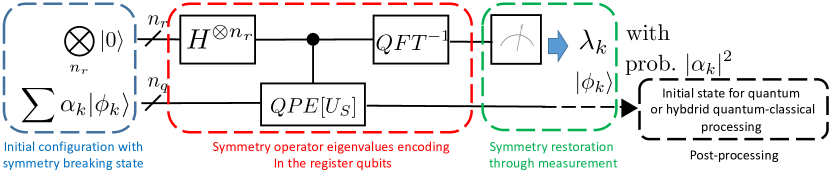
Figure 1: Illustration of the protocol proposed here to prepare a strongly entangled state in a quantum computer using the DSA method. The starting configuration (blue box) is a state $\sum_{k}\alpha_{k}|\phi_{k}\rangle$ and a set of register qubits. The QPE is applied using an operator $U_{S}$ with known discrete spectra (red box). The measurement of register qubits acts as a projector on a set of entangled states that are eigenvectors of the operator $U_{S}$ (green box). The state can then be used for post-processing (black box).

The QPE approach that is based on the Quantum Fourier Transform (QFT) Nie02 ; Hid19 is a practical way to obtain on a quantum computer estimates of the eigenvalues of a unitary operator $U$ acting on $n_{q}$ qubits. This approach makes use of a set of $n_{r}$ register qubits that couple to the working qubits through a repeated applications of controlled-$U$ gates. Denoting by $e^{i{2\pi}\theta_{k}}$ a given eigenvalue of $U$, the QPE approach returns an approximation of the phase, $\tilde{\theta}_{k}$, written as a truncated binary fraction whose precision to describe $\theta_{k}$ depends on $n_{r}$. The QPE is well documented Nie02 , and I only give in Fig. 1 a schematic view of the QPE quantum circuits (additional discussions on QPE can be found in Fan19 ; Ovr03 ; Ovr07 ). I assume that the initial state $|\psi\rangle$ is written in the $n_{q}$ qubits and decomposes as $|\psi\rangle=\sum_{k}\alpha_{k}|\phi_{k}\rangle$ where $|\phi_{k}\rangle$ are eigenvectors associated to the set of phases $\theta_{k}$. After the inverse QFT, the state denoted by $|\psi_{f}\rangle$ becomes:

$$|\psi_{f}\rangle = \sum_{k}\alpha_{k}|\theta_{k}2^{n_{r}}\rangle\otimes|\phi_{k}\rangle.$$ (1)

Here, $|\theta_{k}2^{n_{r}}\rangle$ should be understood as a binary string of $0$ and $1$ that corresponds to the binary fraction of $\theta_{k}$ truncated at the $1/2^{n_{r}}$ term. The eigenvalue estimates are obtained through repeated measurements of the registered qubits. In first approximation, the binary number $\{\theta_{k}2^{n_{r}}\}$ is obtained with a probability $|\alpha_{k}|^{2}$. After the measurement, the state is projected on one of the channels $|\theta_{k}2^{n_{r}}\rangle\otimes|\phi_{k}\rangle$.

In the present work, I propose to use the QPE approach for operators with already known eigenvalues in order to obtain strongly entangled states that are difficult to construct on a classical computer. A hermitian operator $S$ acting on the $n_{q}$ qubits is considered. This operator has a finite discrete set of eigenvalues written in ascending order as $\{\lambda_{0}\leq\cdots\leq\lambda_{M}\}$. I illustrate first the approach to a specific situation where the set of eigenvalues can be connected to a set of integers $\{m_{0}\leq\cdots\leq m_{M}\}$ through a linear relation $\lambda_{k}=am_{k}$, where $a$ is a constant. This example is particularly important because it includes operators that are linked to symmetries such as parity, particle number or angular momentum operators. The generalization to a more general class of operators is discussed below. For the restricted class of operator, I define the unitary operator $U_{S}$ as:

$$U_{S} = \displaystyle\exp\left\{2\pi i\left[\frac{S-\lambda_{0}}{a2^{n_{0}}}\right]\right\}.$$ (2)

The phase associated to each eigenvalue of $U_{S}$ is given by $\theta_{k}=(m_{k}-m_{0})/2^{n_{0}}$. Imposing $\theta_{k}<1$ for all eigenvalues leads to the condition $n_{0}>\ln(m_{k}-m_{0})/\ln 2$. $\theta_{k}$ is then automatically exactly written as a binary fraction truncated at the $n_{0}$ term. When applying the QPE approach for $S$, an optimal choice for the number of register qubits is $n_{r}=n_{0}$ with:

$$n_{r}-1\leq\ln(m_{k}-m_{0})/\ln 2<n_{r}.$$ (3)

In the following applications, the lowest (optimal) value of $n_{r}$ for which the conditions are verified is used as well as $n_{r}=n_{0}$. Taking higher values of $n_{r}$ will lead to useless register qubits. Lower values are a priori possible but this will degrade the selectivity of the states after the measurement. With this optimal choice, the binary strings entering in the registered components of Eq. (1) are directly those corresponding to the $(m_{k}-m_{0})$ values.

The specific choice of $U_{S}$ given by Eq. (1) with the optimal value of $n_{r}$ is particularly suitable for selecting the component $|\phi_{k}\rangle$ associated to the eigenvalue $m_{k}$. Indeed, since the phases $\theta_{k}=(m_{k}-m_{0})/2^{n_{r}}$ exactly write as truncated binary fractions, there is no pollution from other contributions in an ideal quantum device. The ultimate goal of the approach is to obtain after measurements the set of states $|\phi_{k}\rangle$. These states might have highly nontrivial properties depending on the choice of the operator $S$. They can then be used in a second step for further quantum and/or hybrid processing like in the Variational Quantum Eigenvalue (VQE) method Per14 ; McC16 . Since the present approach is based on the use of known discretized spectra for specific operators, I call it Discrete Spectra Assisted (DSA) approach in the following. I illustrate below that symmetry restoration can be achieved using this technology. Interesting discussions on symmetry restoration within quantum computers can be found in Ref. Whi13 ; Tsu20 ; Rya18 ; Yen19 ; Mol16 ; Gar19 . The full protocol proposed here is illustrated in Fig. 1. An initial state with some broken symmetry is prepared on the working qubits. An operator $S$ associated to the symmetry we aim to restore is then chosen and the QPE is applied to $U_{S}$. The register qubits repeated measurements lead to a set of states that respect the symmetry. The last step replaces the symmetry restoration process.

The methodology is illustrated here for the $U(1)$ symmetry associated to particle number. This symmetry breaking, used in the BCS or Hartree-Fock Bogolyubov (HFB) theories, is particularly powerful to account for superfluidity but a precise description of finite systems can only be achieved once the symmetry is restored Bla86 ; Von01 ; Zel03 ; Duk04 ; Bri05 . The goal here is to describe many-body systems, it is then convenient to introduce a single-particle basis associated to creation/annihilation operators $(a^{\dagger}_{j},a_{j})$. The mapping between single-particle states to qubits is made by using the Jordan-Wigner Transformation (JWT) Jor28 ; Lie61 ; Som02 ; See12 ; Dum18 ; Fan19 with the convention:

$$a^{\dagger}_{j} \longrightarrow Q^{+}_{j}\otimes Z^{<}_{j-1},$$ (4)

where $Q^{+}_{j}=\frac{1}{2}\left(X_{j}-iY_{j}\right)$ and $Z^{<}_{j-1}=\bigotimes_{k=1}^{j-1}(-Z_{k})$. $(X_{j}$, $Y_{j}$, $Z_{j})$ together with the identity $I_{j}$ are the standard unary gates applied to the qubit $j$. A natural choice for $S$ for the $U(1)$ symmetry is to take the equivalent to the particle number operator $\hat{N}=\sum_{i}a^{\dagger}_{i}a_{i}$. This operator, counts the number of occupied qubits in the $n_{q}$ basis. With the convention (4), it is given by $\hat{N}=\sum_{j}Q^{+}_{j}Q_{j}=\frac{1}{2}\sum_{j}(I_{j}-Z_{j})$. The operator defined in Eq. (2) is denoted simply as $U_{N}$ below. It can be decomposed as a product of operators acting on each qubit $U_{N}=\prod_{j}U_{j}$ where $U_{j}$ acts on the qubit $j$ and is given by $U_{i}=|0_{i}\rangle\langle 0_{i}|+\exp(i\pi/2^{n_{0}-1})|1_{i}\rangle\langle 1_{i}|$.

The application of the methodology with $U_{N}$ gives access to the probability distribution of the number of occupied qubits in the initial state $|\psi\rangle$, the so-called counting statistics in many-body systems (see for instance Lac20 and ref. therein). For qubits, I call this distribution qubit counting statistics (QCS). Note that the components of the registered qubits prior to he inverse QFT (see Fig. 1) give access to the generating function of the QCS Lac20 .

As a first illustration, some QCS obtained numerically with the IBM Qiskit toolkit Abr19 using the protocol of Fig. 1 are shown in Fig. 2. In these examples, the initial states are obtained from a coherent $Y$-rotation of all working qubits with $|\psi\rangle=\bigotimes_{n_{q}}R^{j}_{Y}(\varphi)|0_{j}\rangle$, where $R^{j}_{Y}(\varphi)=e^{-i\varphi Y_{j}/2}$. In these ideal calculation, I numerically obtained that the QCS probability $P(A)$ to have $A$ occupied qubits in the $n_{q}$ qubits properly identifies with $P(A)=C^{A}_{n_{q}}p^{A}(1-p)^{n_{q}-A}$ where $p=\sin^{2}(\varphi/2)$.

In panels (b)-(c) of Fig. 2, results of the DSA method obtained with a real 5-qubit quantum device are also shown in blackand compared to the ideal case. Deviations from the ideal quantum emulator case sign the effect of noise. Nevertheless, the fact that the trends in the QCS are globally reproduced is rather encouraging for the future use of the approach in the NISQ (Noisy Intermediate-Scale Quantum) context. Note that, I also performed tests on the 15-qubit device provided in IBM Q and the results were essentially compatible with a white noise.

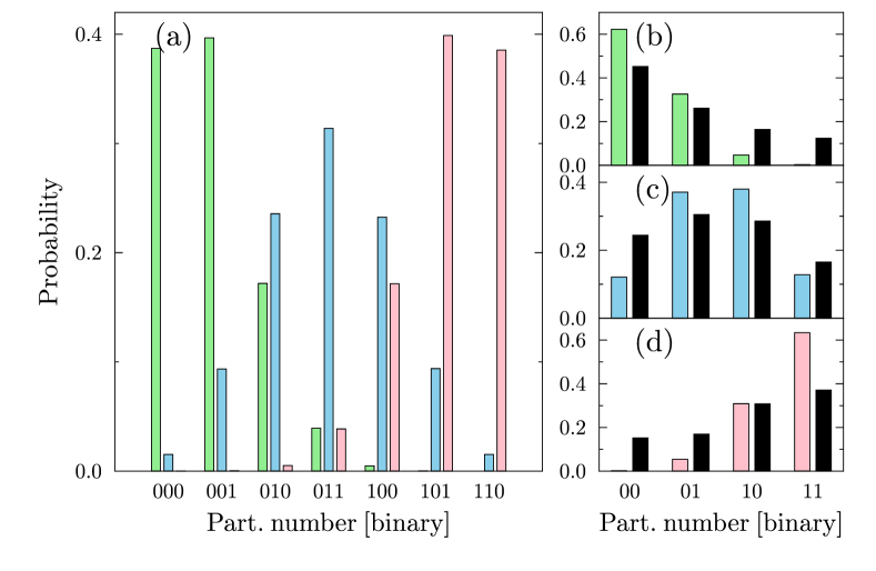
Figure 2: (a) Illustration of the QCS obtained using the DSA approach with the $U_{N}$ operator for the state $|\psi\rangle=\bigotimes_{n_{q}}R^{j}_{Y}(\varphi)|0_{j}\rangle$ for $n_{q}=6$ and with $\varphi=\pi/4$ (green), $\varphi=\pi/2$ (blue) and $\varphi=3\pi/4$ (pink). The $x$-axis corresponds to the binary fraction $A/2^{n_{r}}$ where $A$ is the particle number. In this illustration, $n_{r}=3$ and for instance $A=6$ particles give $6/8=1/2+1/4+0/8\equiv[110]$. In panels (b), (c) and (d) the results of the DSA method obtained with the Qiskit software are shown for $n_{q}=3$ and $n_{r}=2$ for $\varphi=\pi/4$, $\varphi=\pi/2$ and $\varphi=3\pi/4$, respectively. In these panels, the results obtained using the IBM Q 5-qubits ’ibmq_vigo’ real device with 2048 events are systematically shown in black.

With the aim of (i) validating the full method including the post-processing after measurement and (ii) illustrating the powerfulness of the approach, I apply the technique to describe a set of $n_{q}$ fermions interacting through the pairing Hamiltonian Von01 ; Zel03 ; Duk04 ; Bri05 :

$$H_{\rm P} = \sum_{i>0}\varepsilon_{i}(a^{\dagger}_{i}a_{i}+a^{\dagger}_{\bar{i}}a_{\bar{i}})-g\sum_{i,j>0}a^{\dagger}_{i}a^{\dagger}_{\bar{i}}a_{\bar{j}}a_{j}.$$ (5)

$(i,{\bar{i}})$ denotes a pair of time-reversed states, and $i>0$ means that summations are made on pair labels. Note that here $(i,\bar{i})$ labels pair of states in the Fermion Fock space. The Hamiltonian is highly non-local since each pair interacts with all other pairs. It was already considered in Ref. Ovr07 for quantum computation using the standard QPE technique. The Hilbert space is mapped to a set of qubits $n=1,\cdots,n_{q}$ using the JWT technique. By convention, it is assumed here that if $i$ is described by the qubit $n$, then its time-reversed state ${\bar{i}}$ is described by the qubit $n+1$, such that $a^{\dagger}_{i}a^{\dagger}_{\bar{i}}\rightarrow Q^{+}_{n}Q^{+}_{n+1}$.

I consider below the degenerate case $({\varepsilon_{i}}={\varepsilon}=0)$ for which the energy of the eigenstates with $A$ particles is known analytically and is given by Bri05 :

$$E/g=-\frac{1}{4}(A-\nu)(2n_{q}-A-\nu-2).$$ (6)

This equation holds for odd or even particle numbers. $\nu$ denotes the number of broken pairs $(i,\bar{i})$ in the eigenstates, that is the so-called seniority (for more details on the seniority see for instance Rin81 ; Bri05 ). Increasing the values of $\nu$ gives access to the different excited-state energies for a fixed $A$.

.

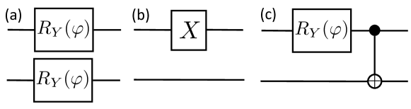
Figure 3: Illustration of the 3 circuits used in the text to prepare a pair of time-reversed states.

We first need to specify a convenient initial state $|\psi\rangle$. Guided by the BCS/HFB approach Bla86 , a Gaussian state breaking the $U(1)$ symmetry is considered:

$$|\psi\rangle = \prod_{n>0}e^{i\varphi\left(X_{n}Y_{n+1}+Y_{n}X_{n+1}\right)/2}|-\rangle,$$ (7)

where $|-\rangle=|0,\cdots,0\rangle_{n_{q}}$. A general quantum circuit to obtain this state is given in Jia18 (see also Ver09 ). A simpler circuit is used here noting that:

$$|\psi\rangle=\prod_{n}\left[\cos\left(\frac{\varphi}{2}\right)I_{n}\otimes I_{n+1}+\sin\left(\frac{\varphi}{2}\right)Q^{+}_{n}Q^{+}_{n+1}\right]|-\rangle,$$ (8)

where the product is made on even $n$ only. For a given pair, the state $[\cos\left(\varphi/2\right)|00\rangle+\sin\left(\varphi/2\right)|11\rangle]$ is produced. This state, interpreted as a generalized Bell state, is obtained by applying the simple circuit shown in Fig. 3-(c) to all $(n,n+1)$ pairs.

The DSA approach is applied to the state (8) using $U_{N}$ as a filter. For each measurement, labeled by $(\lambda)$, a specific string of $0$ or $1$ is measured for the register qubits. The measured binary string equals $A^{(\lambda)}/2^{n_{r}}$ where $A^{(\lambda)}$ is the particle number of the event. After the measurement, a set of states $|\psi^{(\lambda)}_{f}\rangle$ is obtained in the working qubit basis, each of them having exactly the particle number $A^{(\lambda)}$. A hybrid calculation is then performed by computing on a classical computer the energy $E^{(\lambda)}=\langle\psi^{(\lambda)}_{f}|H_{P}|\psi^{(\lambda)}_{f}\rangle$. The statistical ensemble of energies obtained in a single run is displayed in Fig. 4. The ground-state (GS) energies of all even particle numbers as given by Eq. (6) with $\nu=0$ are recovered in this run illustrating the advantage of quantum parallelism.

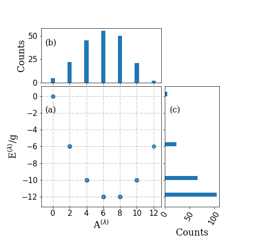
Figure 4: Panel (a): Correlation between the energies $E^{(\lambda)}$ and particle number $A^{(\lambda)}$ obtained with the IBM Qiskit emulator Abr19 for $200$ events using the DSA method for $n_{q}=12$ Qubits ($6$ pairs) with 3 register qubits and $\varphi=\pi/2$. The distribution of counts for the particle number and energies are shown respectively in panels (b) and (c).

For the degenerate case, unless the specific situation $\varphi=k\pi$ is considered, all eigenvalues are obtained from a single-value of $\varphi$ and only the probability distributions displayed in panels (b) and (c) of Fig. 4 depend on $\varphi$. This method can be generalized to treat a more complex pairing Hamiltonian by allowing $Y$-rotation with different angles $\varphi_{n}$ for different pairs. The set of $\{\varphi_{n}\}$ can then be used as variational parameters to construct highly entangled states that can be used for instance in a VQE algorithm.

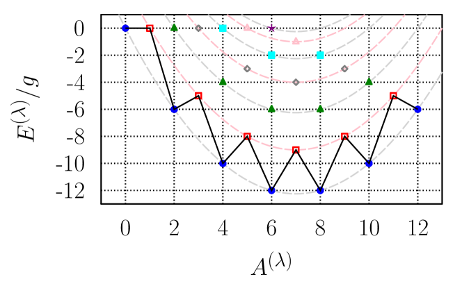
Figure 5: Energies obtained for $n_{q}=12$ by replacing the circuits (c) displayed in Fig. 3 by the circuit (b) for an increasing number of pairs. The number of replacements then corresponds to the seniority value. Results have been obtained using the IBM Qiskit simulator Abr19 with $200$ events and $n_{q}=12$ working qubits. For even particle numbers, $\nu=0$ (blue filled circles), $2$ (green filled triangles), $4$ (cyan filled squares), $6$ (purple star) are shown. For odd particle numbers, $\nu=1$ (open red squares), $3$ (open gray diamond), $5$ (open pink triangle) are shown. The dashed lines correspond to the analytical result (6) with different seniority values. Even (resp. odd) seniorities are shown with gray (resp. pink) dashed lines. The black line connects the results obtained by replacing for one pair the circuit (c) by the circuit (a).

I finally show in Fig. 5 that the blocking technique sometimes used in superfluid systems Rin80 can easily be transposed to qubit systems to access excited states in odd or even systems. One or several pairs can be broken by replacing the circuits (c) displayed in Fig. 3 by the circuit (b). The correlations between the $A^{(\lambda)}$ and $E^{(\lambda)}$ obtained by breaking from $1$ to $n_{q}/2$ pairs is shown in Fig. 5. Imposing one broken pair gives the GS energy of odd systems while breaking two pairs gives the first excited state in even system. Breaking more and more pairs finally gives the full odd-even spectra. There exists a large flexibility to be explored to access selected parts of the spectra with various particle numbers. I show in Fig. 5 that the GS energy of both odd and even systems can be simultaneously obtained by replacing simply for one pair the circuit (c) by the circuit (a) of Fig. 3.

In summary, an approach to obtain strongly entangled states that might be useful to describe interacting systems on a quantum computer is presented here. Starting from an operator having a known discrete spectra, the QPE approach is used to obtain an ensemble of entangled states. When the operator is related to a symmetry of the Hamiltonian, the protocol proposed here can be interpreted as a quantum computer equivalent to the SB-SR approach that is a powerful tool to describe static and dynamical properties of interacting mesoscopic systems Bla86 ; Rin81 ; Hen14 ; Qiu19 ; Gam12 ; Reg19 ; Kha20 . The DSA method can be applied even if the linear condition $\lambda_{k}=am_{k}$ is relaxed by introducing the operator $U_{S}=\displaystyle\exp\left\{2\pi i(S-\lambda_{0})/\Delta\right\}$ with $\Delta=\lambda_{M}-\lambda_{0}+\varepsilon$. $\varepsilon$ is a small number insuring that the eigenvalues of $U_{S}$, given by $e^{i2\pi\theta_{k}}$, verify $\theta_{k}=(\lambda_{k}-\lambda_{0})/\Delta<1$. Since in general the $\{\theta_{k}\}$ will not be written exactly as a truncated binary fraction, the application of the DSA approach is anticipated to require more register qubits in order to discriminate all channels. One can introduce the quantity $\theta_{d}=d/\Delta$ and its binary fraction $\theta_{d}=0.x_{1}x_{2}\cdots$, where $d=\min_{0\leq k<M}(\lambda_{k+1}-\lambda_{k})$. Assuming that $x_{m}$ is the first non-zero value in the binary fraction expansion, a minimal condition is then $n_{r}>m$. Multiple projections of commuting operators can also be made at the price of increasing the number of register qubits. The restoration of broken symmetries is a pillar in the treatment of complex interacting systems beyond the perturbative regime. The state-of-the-art is to use it in the Variation-After-Projection (VAP) version Rin81 ; Ben03 ; Rob19 or used to propose novel many-body techniques Hen14 ; Rip17 ; Rip18 . In the VAP and in these new techniques, the projection becomes intractable especially when several symmetries are simultaneously restored as it may happen for example in nuclei. The possibility to perform multiple projections on a quantum computers open perspectives in this context.

References

- (1) M. A. Nielsen and I. L. Chuang. Quantum information and quantum computation., Cambridge University Press (2000) vol. 2, no 8, p. 23.
- (2) J. D. Hidary, Quantum Computing: An Applied Approach, Springer International Publishing, (2019).
- (3) Jarrod R McClean et al, OpenFermion: the electronic structure package for quantum computers, Quantum Sci. Technol. 5, 034014 (2020). McClean, Jarrod R., et al., OpenFermion: the electronic structure package for quantum computers, arXiv:1710.07629 (2017).
- (4) Guido Fano, S. M. Blinder, Mathematical Physics in Theoretical Chemistry, 377 (2019).
- (5) Yudong Cao et al, Quantum Chemistry in the Age of Quantum Computing, Chem. Rev. 119, 19, 10856 (2019).
- (6) Sam McArdle, Suguru Endo, Alán Aspuru-Guzik, Simon C. Benjamin, and Xiao Yuan Rev. Mod. Phys. 92, 015003 (2020).
- (7) Bela Bauer, Sergey Bravyi, Mario Motta, Garnet Kin-Lic Chan, arXiv:2001.03685.
- (8) B. P. Lanyon, J. D. Whitfield, G. G. Gillett, M. E. Goggin, M. P. Almeida, I. Kassal, J. D. Biamonte, M. Mohseni, B. J. Powell, M. Barbieri, et al., Nature chemistry 2, 106 (2010).
- (9) R. Babbush, J. McClean, D. Wecker, A. Aspuru-Guzik, N. Wiebe, Phys. Rev. A 91, 022311 (2015).
- (10) P. J. O’Malley et al., Phys. Rev. X 6, 031007 (2016).
- (11) J. I. Colless, V. V. Ramasesh, D. Dahlen, M. S. Blok, M. E. Kimchi-Schwartz, J. R. McClean, J. Carter, W. A de Jong, and I. Siddiqi, Phys. Rev. X 8, 011021 (2018).
- (12) Cornelius Hempel, Christine Maier, Jonathan Romero, Jarrod McClean, Thomas Monz, Heng Shen, Petar Jurcevic, Ben P. Lanyon, Peter Love, Ryan Babbush, Alán Aspuru-Guzik, Rainer Blatt, and Christian F. Roos Phys. Rev. X 8, 031022 (2018).
- (13) A. Macridin, P. Spentzouris, J. Amundson, R. Harnik, Phys. Rev. Lett. 121, 110504 (2018).
- (14) E.F. Dumitrescu, A.J. McCaskey, G. Hagen, G. R. Jansen, T.D. Morris, T. Papenbrock, R.C. Pooser, D.J. Dean, and P. Lougovski, Phys. Rev. Lett. 120, 210501 (2018).
- (15) Hsuan-Hao Lu, Natalie Klco, Joseph M. Lukens, Titus D. Morris, Aaina Bansal, Andreas Ekström, Gaute Hagen, Thomas Papenbrock, Andrew M. Weiner, Martin J. Savage, and Pavel Lougovski Phys. Rev. A 100, 012320 (2019)
- (16) A. Roggero and J. Carlson, Phys. Rev. C 100, 034610 (2019)
- (17) Weijie Du, James P. Vary, Xingbo Zhao, Wei Zuo, arXiv:2006.01369.
- (18) N. Klco et al., Phys. Rev. A 98, no. 3, 032331 (2018)
- (19) N. Klco and M. J. Savage, Phys. Rev. A 99, 052335 (2019)
- (20) A. Alexandru et al. , Phys. Rev. Lett. 123, 090501 (2019)
- (21) H. Lamm et al., Phys. Rev. D 100, 034518 (2019)
- (22) P. Ring and P. Schuck, The Nuclear Many-Body Problem (Springer-Verlag, New-York, 1980).
- (23) J. P. Blaizot and G. Ripka, Quantum Theory of Finite Systems (MIT Press, Cambridge, 1986).
- (24) L. M. Robledo, , T. R. Rodríguez, and R. R. Rodríguez-Guzmán, Journal of Physics G: Nuclear and Particle Physics 46, 013001 (2018).
- (25) M. Bender, P.-H. Heenen, and P.-G. Reinhard, Rev. Mod. Phys. 75, 121 (2003).
- (26) E. Ovrum. Quantum computing and many-body physics. Master’s thesis, University of Oslo, (2003).
- (27) Ovrum E, Hjorth-Jensen M. Quantum computation algorithm for many-body studies, arXiv:0705.1928v1.
- (28) Alberto Peruzzo, Jarrod McClean, Peter Shadbolt, Man-Hong Yung, Xiao-Qi Zhou, Peter J. Love, Alán Aspuru-Guzik and Jeremy L. O’Brien, Nature Communications 5, 4213 (2014).
- (29) Jarrod R McClean, Jonathan Romero, Ryan Babbush and Alán Aspuru-Guzik, New J. of Phys. 18, 023023 (2016).
- (30) James Daniel Whitfield, J. Chem. Phys. 139, 021105 (2013).
- (31) Takashi Tsuchimochi and Yuto Mori, arXiv:2004.12024.
- (32) Ilya G. Ryabinkin and Scott N. Genin, arxiv:1812.09812v1
- (33) Tzu-Ching Yen, Robert A. Lang, and Artur F. Izmaylov, arXiv:1905.08109v2
- (34) N. Moll, A. Fuhrer, P. Staar, and I. Tavernelli, J. Phys. A: Math. Theor. 49, 295301 (2016).
- (35) Bryan T. Gard, Linghua Zhu, George S. Barron, Nicholas J. Mayhall, Sophia E. Economou, and Edwin Barnes, arXiv:1904.10910v3
- (36) J. von Delft and D. C. Ralf, Phys. Rep. 345, 61 (2001).
- (37) V. Zelevinsky and A. Volya, Phys. of Atomic Nuclei 66, 1781 (2003).
- (38) J. Dukelsky, S. Pittel, and G. Sierra, Rev. Mod. Phys. 76, 643 (2004).
- (39) D. M. Brink and R. A. Broglia, Nuclear Superfluidity: Pairing in Finite Systems (Cambridge University Press, 2005).
- (40) P. Jordan and E. Wigner, Zeitschrift für Physik 47, 631 (1928).
- (41) Elliott Lieb, Theodore Schultz, Daniel Mattis, Ann. of Phys. 16, 407 (1961).
- (42) R. Somma, G. Ortiz, J. E. Gubernatis, E. Knill, and R. Laflamme Phys. Rev. A 65, 042323 (2002).
- (43) J. T. Seeley, M. J. Richard, and P. J. Love, J. Chem. Phys. 137, 224109 (2012).
- (44) Denis Lacroix and Sakir Ayik, Phys. Rev. C 101, 014310 (2020).
- (45) Héctor Abraham et al [Qiskit collaboration], Qiskit: An Open-source Framework for Quantum Computing, https://qiskit.org/ (2019), DOI: 10.5281/zenodo.2562110
- (46) P. Ring and P. Schuck, The Nuclear Many-Body Problem (Springer-Verlag, Berlin, 2000).
- (47) Zhang Jiang, Kevin J. Sung, Kostyantyn Kechedzhi, Vadim N. Smelyanskiy, and Sergio Boixo Phys. Rev. Applied 9, 044036 (2018).
- (48) F. Verstraete, J. I. Cirac, and J. I. Latorre, Phys. Rev. A 79, 032316 (2009).
- (49) Thomas M. Henderson, Gustavo E. Scuseria, Jorge Dukelsky, Angelo Signoracci, and Thomas Duguet Phys. Rev. C 89, 054305 (2014) .
- (50) Y. Qiu, T. M. Henderson, T. Duguet, and G. E. Scuseria Phys. Rev. C 99, 044301 (2019).
- (51) Armin Khamoshi, Thomas Henderson, Gustavo Scuseria, arXiv:1909.06345.
- (52) Danilo Gambacurta and Denis Lacroix, Phys. Rev. C 85, 044321 (2012).
- (53) David Regnier and Denis Lacroix, Phys. Rev. C 99, 064615 (2019).
- (54) L. M. Robledo, T. R. Rodríguez, R. R. Rodríguez-Guzmán, J. Phys. G 46, 013001 (2019).
- (55) J. Ripoche, D. Lacroix, D. Gambacurta, J.-P. Ebran, and T. Duguet, Phys. Rev. C 95, 014326 (2017)
- (56) J. Ripoche, T. Duguet, J.-P. Ebran, and D. Lacroix, Phys. Rev. C 97, 064316 (2018).