The SOFIA Massive (SOMA) Star Formation Survey. III.
From Intermediate- to High-Mass Protostars

Abstract

We present $\sim 10-40\,\mu$m SOFIA-FORCAST images of 14 intermediate-mass protostar candidates as part of the SOFIA Massive (SOMA) Star Formation Survey. We build spectral energy distributions (SEDs), also utilizing archival Spitzer, Herschel and IRAS data. We then fit the SEDs with radiative transfer (RT) models of Zhang & Tan (2018), based on Turbulent Core Accretion theory, to estimate key protostellar properties. With the addition of these intermediate-mass sources, SOMA protostars span luminosities from $\sim 10^{2}-10^{6}\>L_{\odot}$, current protostellar masses from $\sim 0.5-30\>M_{\odot}$ and ambient clump mass surface densities, $\Sigma_{\rm cl}$ from $0.1-3\>{\rm{g\>cm}^{-2}}$. A wide range of evolutionary states of the individual protostars and of the protocluster environments are also probed. We have also considered about 50 protostars identified in Infrared Dark Clouds and expected to be at the earliest stages of their evolution. With this global sample, most of the evolutionary stages of high- and intermediate-mass protostars are probed. From the best fitting models, there is no evidence of a threshold value of protocluster clump mass surface density being needed to form protostars up to $\sim 25\>M_{\odot}$. However, to form more massive protostars, there is tentative evidence that $\Sigma_{\rm{cl}}$ needs to be $\gtrsim 1\>{\rm{g\,cm}}^{-2}$. We discuss how this is consistent with expectations from core accretion models that include internal feedback from the forming massive star.

cont#1 (cont.)#2#3

1 Introduction

Table 1: SOFIA FORCAST Observations: Observation Dates & Exposure Times (seconds)

Source	R.A.(J2000)	Decl.(J2000)	$d$ (kpc)	Obs. Date	7.7$\>{\rm\mu m}$	19.7$\>{\rm\mu m}$	31.5$\>{\rm\mu m}$	37.1$\>{\rm\mu m}$
S235	05h40m52$\fs$4	$+$35$\arcdeg$41$\arcmin$30$\arcsec$	1.8	2016 Sep 20	404	779	642	1504
IRAS 22198+6336	22h21m26$\fs$68	$+$63$\arcdeg$51$\arcmin$38$\farcs$2	0.764	2015 Jun 05	278	701	482	743
NGC 2071	05h47m04$\fs$741	$+$00$\arcdeg$21$\arcmin$42$\farcs$96	0.39	2018 Sep 08	492	1319	825	2020
Cepheus E	23h03m12$\fs$8	$+$61$\arcdeg$42$\arcmin$26$\arcsec$	0.73	2015 Nov 04	281	899	818	281
L1206	22h28m51$\fs$41	$+$64$\arcdeg$13$\arcmin$41$\farcs$1	0.776	2015 Nov 20	116	308	162	630
IRAS 22172+5549	22h19m09$\fs$478	$+$56$\arcdeg$05$\arcmin$00$\farcs$370	2.4	2015 Jun 03	337	664	386	466
IRAS 21391+5802	21h40m41$\fs$90	$+$58$\arcdeg$16$\arcmin$12$\farcs$3	0.75	2015 Nov 06	334	806	488	1512

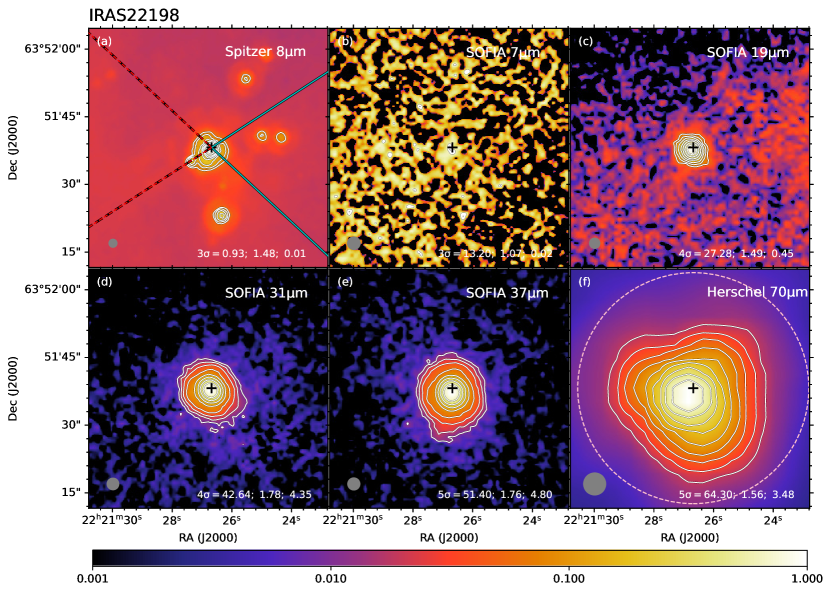
Figure 2: Multi-wavelength images of IRAS 22198+6336, following the format of Figure 1. The black cross in all panels denotes the position of the 3.6 cm source in Sánchez-Monge et al. (2008) at R.A.(J2000) = 22^h21^m26$\fs$68, Decl.(J2000) = $+$63$\arcdeg$51$\arcmin$38$\farcs$2. The lines in panel (a) show the orientation of outflow axes, with the solid spans tracing blue-shifted direction and the dashed spans red-shifted direction. The outflow axis angles are from the CO(1-0) outflow emission of Sánchez-Monge et al. (2010).

Note. — The source positions listed here are the same as the positions of the black crosses denoting the radio continuum peak (mm continuum peak in Cep E and L1206 A, and MIR peak in IRAS22172 MIR2) in each source in Figures 1-7. Source distances are from the literature, as discussed below.

Intermediate-mass (IM) protostars are important as representatives of the transition between the extremes of low- (i.e., $\lesssim 2\>M_{\odot}$) and high- (i.e., $\gtrsim 8\>M_{\odot}$) mass star formation. These objects are relatively rare compared to their low-mass counterparts and tend to be located at greater distances. They are precursors of Herbig Ae and Be stars. The immediate environments of IM protostars can appear quite complex, with extended emission often resolved into multiple sources when observed at high resolution (e.g., G173.58+2.45, Shepherd & Watson 2002). However, there are also examples with relatively simpler, more isolated morphologies (e.g., Cep E, Moro-Martín et al. 2001). Observations of IM protostars indicate that they share some similar physical properties as low-mass protostars, such as circumstellar disks (e.g., Zapata et al. 2007; Sánchez-Monge et al. 2010; van Kempen et al. 2012; Takahashi et al. 2012) and collimated molecular outflows (e.g., Gueth et al. 2001; Beltrán et al. 2008, 2009; Palau et al. 2010; Velusamy et al. 2011), but with the latter being more powerful when driven from IM protostars. Furthermore, IM protostars also share many characteristics with their higher-mass counterparts, such as correlations between the outflow kinematics and the properties of their driving sources (e.g., Cabrit & Bertout 1992; Bontemps et al. 1996; Wu et al. 2004; Hatchell et al. 2007; Beltrán et al. 2008), and hot core chemistry (e.g., Fuente et al. 2005; Neri et al. 2007; Sánchez-Monge et al. 2010). Thus, the observational evidence suggests that intermediate-mass protostars form in a similar way as low-mass protostars, and that this formation mechanism is also shared with at least early B-type or late O-type protostars (Beltrán 2015).

In this paper, we study a sample of 14 IM protostars selected from the SOFIA Massive (SOMA) Star Formation Survey (PI: Tan), which aims to characterize a sample of $\gtrsim$ 50 high- and intermediate-mass protostars over a range of evolutionary stages and environments with their $\sim$ 10 to 40 $\mu$m images observed with the SOFIA-Faint Object infraRed CAmera for the SOFIA Telescope (FORCAST) instrument. In Paper I of the survey (De Buizer et al. 2017), the first eight sources were presented, which were mostly massive protostars. In Paper II (Liu et al. 2019), seven especially luminous sources were presented, corresponding to some of the most massive protostars in the survey. Thus the IM sample presented here, which consists of 7 new target regions from which 12 protostars have been studied plus 2 more protostars extracted as secondary sources from Papers I and II target regions, serves to extend the luminosity and mass range of the survey sample down to lower values.

Our approach is to follow the same methods developed in Papers I and II to build the spectral energy distributions (SEDs) of the sources. As before, we then fit these SEDs with the Zhang & Tan (2018, hereafter ZT18) protostellar radiative transfer (RT) models to estimate intrinsic source properties. In this way, all the protostars are analyzed in an uniform way. Finally, we search for trends in source properties among the overall SOMA sample of 29 sources that have been so far analyzed in Papers I, II and III.

The observations and data utilized in this paper are described in §2. The analysis methods are summarized in §3. We present the MIR imaging and SED fitting results in §4 and discuss these results and their implications in §5. A summary is given in §6.

2 Observations

The following seven target regions were observed by SOFIA (Young et al. 2012) with the FORCAST instrument (Herter et al. 2013) (see Table 1): S235, IRAS 22198+6336, NGC 2071, Cep E, L1206 (A and B), IRAS22172+5549 (MIR 1, MIR 2, and MIR 3), IRAS 21391+5802 (BIMA 2, BIMA 3, and MIR 48). The angular resolutions of the SOFIA-FORCAST images are 2.7″ at 7 $\rm\mu m$, 2.9″ at 11 $\rm\mu m$, 3.3″ at 19 $\rm\mu m$, 3.4″ at 31 $\rm\mu m$, and 3.5″ at 37 $\rm\mu m$. We also fit the SEDs of two more sources G305.20+0.21 A (hereafter, G305 A) and IRAS 16562-3959 N (hereafter, IRAS 16562 N), which are secondary sources near primary targets of Paper II. Thus a total of 14 protostars will be analyzed here for the first time as SOMA Survey sources.

In addition to SOFIA observations, for all objects, we also retrieve publicly-available images of Spitzer/IRAC (Fazio et al. 2004) at 3.6, 4.5, 5.8 and 8.0 $\mu$m from the Spitzer Heritage Archive, Herschel/PACS and SPIRE (Griffin et al. 2010) at 70, 160, 250, 350 and 500 $\mu$m from the Herschel Science Archive, and Higher Resolution IRAS Images (HIRES) (Neugebauer et al. 1984) at 60, 100 $\mu$m from the NASA/IPAC Infrared Science Archive.

The calibration and astrometry methods are the same as those of Paper II, except that for Cep E and IRAS 21391 we use the SOFIA 19 $\mu$m image instead of 7 $\mu$m to calibrate the other SOFIA images and the Herschel images given the high noise level in their 7 $\mu$m images. For SOFIA observations the calibration error is estimated to be in the range $\sim$ 3% - 7%. The astrometric precision is about 0.1″ for the SOFIA 7 $\mu$m image, 0.4″ for longer wavelength SOFIA images, and 1$\arcsec$ for Herschel images. Note that we use HIRES results of the IRAS data to achieve a resolution $\sim$ 1′. The astrometric precision is about 20 - 30″. Fluxes measured from HIRES agree with those of the Point Source Catalog (PSC2) to within 20% and ringing (a ring of lower level flux may appear around a point source) can contribute up to another 10% uncertainty in the measurement of the background subtracted flux of the source. Thus the total uncertainty, summing in quadrature, is 23%. Near-Infrared (NIR) images from the Wide Field Camera (WFC)/ UKIRT InfraRed Deep Sky Survey (UKIDSS) (Lawrence et al. 2007) surveys and the Two Micron All Sky Survey (2MASS) Atlas images (Skrutskie et al. 2006) are also used to investigate the environments of the protostellar sources and look for association with the MIR counterparts.

3 Methods

We follow the methods described in Papers I and II to construct the SEDs (see §3 of Papers I and II for more detailed discussion). In summary, fixed circular aperture, background-subtracted photometry is estimated from MIR to FIR wavelengths for the sources. The aperture radius is chosen with reference to the 70 $\rm\mu m$ Herschel-PACS source morphology, when available (else the 37 $\rm\mu m$ SOFIA-FORCAST source morphology), with the goal of enclosing the majority of the flux, while avoiding contamination from surrounding sources.

We also follow the methods of Papers I and II to fit the SEDs with ZT18 protostellar radiative transfer models. For IRAS 22198, NGC 2071, Cep E, G305 A, IRAS 16562 N, which have Herschel data, we do not use IRAS data for the SED fitting. For L1206, our SOFIA images show that L1206 A is much brighter than L1206 B at long wavelengths: e.g., at 37 $\mu$m L1206 A contributes 96% of the total flux. Thus we assume L1206 A is the main source at wavelengths longer than 37 $\mu$m and use the IRAS flux densities at 60 $\mu$m and 100 $\mu$m as a normal data point for the SED fitting of L1206 A and upper limits for the SED fitting of L1206 B. For the other sources, IRAS data are used as upper limits given its resolution and aperture size.

There are a few special cases for the SED fitting. For G305 A, at wavelengths shorter than 8 $\mu$m there is hardly any emission and the local noise leads to a negative flux measurement at 7 $\mu$m. Thus we use the non-background subtracted fluxes as upper limits at 3.6, 4.5, 5.8 and 8.0 $\mu$m. In the IRAS 16562 region, the flux densities at wavelengths longer than 250 $\mu$m are dominated by the main source in Paper II, thus the background subtracted flux for IRAS 16562 N is negative at these wavelengths because of the contamination of the main source. Thus we use the non-background subtracted fluxes as upper limits at 250, 350 and 500 $\mu$m.

4 Results

Table 2 lists the types of multi-wavelength data available for each source, the flux densities derived, and the aperture sizes adopted. $F_{\lambda,\rm fix}$ is the flux density derived with a fixed aperture size and $F_{\lambda,\rm var}$ is the flux density derived with a variable aperture size. The value of flux density listed in the upper row of each source is derived with background subtraction, while that derived without background subtraction is listed in parentheses in the lower row. The SOFIA images for each source are presented in §4.1. General results of the SOFIA imaging are summarized in §4.2. The SEDs and fitting results are presented in §4.3.

Table 2: Integrated Flux Densities

Facility	$\lambda$	Fλ,fix	Fλ,var	Rap	Fλ,fix	Fλ,var	Rap	Fλ,fix	Fλ,var	Rap	Fλ,fix	Fλ,var	Rap	Fλ,fix	Fλ,var	Rap	Fλ,fix	Fλ,var	Rap
	($\mu$m)	(Jy)	(Jy)	($\arcsec$)	(Jy)	(Jy)	($\arcsec$)	(Jy)	(Jy)	($\arcsec$)	(Jy)	(Jy)	($\arcsec$)	(Jy)	(Jy)	($\arcsec$)	(Jy)	(Jy)	($\arcsec$)
		S235			IRAS 22198			NGC2071			Cep E			L1206 A			L1206 B
Spitzer/IRAC	3.6	0.50	0.48	9.0	0.05	0.01	6.6	0.34	0.12	3.6	0.05	0.06	28.0	0.11	0.13	12.0	…	…	…
		(0.54)	(0.51)		(0.08)	(0.01)		(0.38)	(0.14)		(0.06)	(0.08)		(0.12)	(0.15)
Spitzer/IRAC	4.5	0.46	0.44	9.0	0.13	0.03	4.8	1.24	0.54	3.6	0.17	0.24	28.0	0.25	0.30	12.0	…	…	…
		(0.51)	(0.47)		(0.15)	(0.04)		(1.32)	(0.63)		(0.18)	(0.25)		(0.27)	(0.33)
Spitzer/IRAC	5.8	1.99	1.90	9.0	0.20	0.08	5.4	2.54	1.59	3.6	0.23	0.27	28.0	0.28	0.33	12.0	2.10	2.10	10.0
		(2.24)	(2.06)		(0.43)	(0.10)		(2.78)	(1.71)		(0.31)	(0.38)		(0.33)	(0.41)		(2.19)	(2.19)
SOFIA/FORCAST	7.7	6.39	6.22	9.0	0.85	0.20	5.4	5.58	4.04	3.8	0.17	0.23	6.0	0.12	0.30	4.6	2.21	1.53	5.0
		(6.24)	(6.13)		(1.41)	(0.29)		(5.53)	(4.32)		(0.19)	(0.20)		(0.19)	(0.27)		(2.04)	(1.65)
Spitzer/IRAC	8.0	6.12	5.83	9.0	0.23	0.15	6.6	6.08	4.09	3.8	0.31	0.34	28.0	0.21	0.24	12.0	3.45	3.45	10.0
		(6.76)	(6.25)		(0.84)	(0.20)		(6.48)	(4.34)		(0.56)	(0.70)		(0.29)	(0.37)		(3.59)	(3.59)
SOFIA/FORCAST	19.7	33.66	32.64	9.0	10.35	5.40	7.0	86.65	63.79	3.8	1.41	1.69	6.0	2.11	1.82	6.2	4.70	4.32	8.0
		(34.25)	(33.28)		(15.13)	(6.17)		(86.97)	(66.50)		(1.43)	(1.56)		(2.42)	(2.09)		(4.08)	(4.05)
SOFIA/FORCAST	31.5	70.87	70.87	12.0	91.08	77.83	9.2	310	169	3.8	20.50	16.73	7.7	65.17	63.01	7.7	5.50	5.50	10.0
		(72.92)	(72.92)		(90.51)	(80.47)		(318)	(190)		(21.61)	(17.47)		(67.06)	(65.13)		(3.37)	(3.37)
SOFIA/FORCAST	37.1	84.95	84.95	12.0	132	111	9.2	375	176	3.8	25.89	23.56	7.7	116	116	9.0	7.20	7.20	10.0
		(88.39)	(88.39)		(130)	(115)		(382)	(205)		(25.40)	(24.02)		(117)	(117)		(5.09)	(5.09)
IRAS	60.0	…	2281	186.6	…	224	109.2	…	1146	200.0	…	66.13	141.0	…	432	125.2	…	432	125.2
		…	(2386)		…	(235)		…	(1213)		…	(63.58)		…	(445)		…	(445)
Herschel/PACS	70.0	…	…	…	449	449	25.6	694	694	9.6	99	99	23.0	…	…	…	…	…	…
					(471)	(471)		(753)	(753)		(103)	(103)
IRAS	100.0	…	2897	244.5	…	525	180.0	…	2559	205.1	…	152	177.5	…	880	215.7	…	880	215.7
		…	(3255)		…	(666)		…	(2879)		…	(137)		…	(947)		…	(947)
Herschel/PACS	160.0	…	…	…	360	360	25.6	421	421	9.6	127	127	23.0	…	…	…	…	…	…
					(401)	(401)		(572)	(572)		(143)	(143)
Herschel/SPIRE	250.0	…	…	…	190	190	25.6	…	…	…	71.43	71.43	23.0	…	…	…	…	…	…
					(217)	(217)					(87.60)	(87.60)
Herschel/SPIRE	350.0	…	…	…	93	93	25.6	…	…	…	29.35	29.35	23.0	…	…	…	…	…	…
					(107)	(107)					(38.37)	(38.37)
Herschel/SPIRE	500.0	…	…	…	35.06	35.06	25.6	…	…	…	7.61	7.61	23.0	…	…	…	…	…	…
					(40.65)	(40.65)					(12.45)	(12.45)

Note. — The value of flux density in the upper row is derived with background subtraction. The value in parentheses in the lower line is the flux density derived without background subtraction.

The center of the aperture used for photometry of the IRAS images is not the same as those used at other wavelengths, but is determined based on the emission of the image alone. See more details in Papers I & II.

Table 2: Integrated Flux Densities (continued)

Facility	$\lambda$	Fλ,fix	Fλ,var	Rap	Fλ,fix	Fλ,var	Rap	Fλ,fix	Fλ,var	Rap	Fλ,fix	Fλ,var	Rap	Fλ,fix	Fλ,var	Rap	Fλ,fix	Fλ,var	Rap	Fλ,fix	Fλ,var	Rap	Fλ,fix	Fλ,var	Rap
	($\mu$m)	(Jy)	(Jy)	($\arcsec$)	(Jy)	(Jy)	($\arcsec$)	(Jy)	(Jy)	($\arcsec$)	(Jy)	(Jy)	($\arcsec$)	(Jy)	(Jy)	($\arcsec$)	(Jy)	(Jy)	($\arcsec$)	(Jy)	(Jy)	($\arcsec$)	(Jy)	(Jy)	($\arcsec$)
		IRAS22172 MIR2			IRAS22172 MIR1			IRAS22172 MIR3			IRAS21391 BIMA2			IRAS21391 BIMA3			IRAS21391 MIR48			IRAS16562 N			G305 A
Spitzer/IRAC	3.6	0.15	0.09	2.4	0.07	0.07	3.6	0.02	0.02	3.6	0.01	0.01	4.6	0.02	0.01	3.6	0.05	0.04	3.6	0.06	0.04	6.0	…	…	12.0
		(0.17)	(0.11)		(0.09)	(0.08)		(0.03)	(0.03)		(0.02)	(0.01)		(0.03)	(0.02)		(0.05)	(0.04)		(0.13)	(0.09)		(0.16)	(0.16)
Spitzer/IRAC	4.5	0.43	0.29	2.4	0.07	0.05	2.4	0.02	0.01	2.4	0.07	0.05	4.6	0.06	0.05	4.5	0.09	0.08	4.5	0.08	0.06	6.0	…	…	12.0
		(0.46)	(0.31)		(0.09)	(0.06)		(0.03)	(0.01)		(0.09)	(0.06)		(0.08)	(0.06)		(0.09)	(0.09)		(0.16)	(0.11)		(0.19)	(0.19)
Spitzer/IRAC	5.8	0.71	0.43	2.4	0.17	0.07	2.4	0.16	0.12	3.6	0.11	0.10	4.6	0.10	0.09	4.5	0.15	0.14	5.4	0.20	0.07	4.5	…	…	12.0
		(0.77)	(0.50)		(0.25)	(0.12)		(0.20)	(0.15)		(0.17)	(0.12)		(0.15)	(0.11)		(0.18)	(0.16)		(0.75)	(0.30)		(1.13)	(1.13)
SOFIA/FORCAST	7.7	0.95	0.69	2.7	0.43	0.58	5.4	0.54	0.54	4.6	0.29	0.13	4.6	0.17	0.10	6.4	0.21	0.26	6.4	0.73	0.16	4.5	…	…	…
		(1.10)	(0.85)		(0.71)	(0.88)		(0.70)	(0.70)		(0.39)	(0.22)		(0.37)	(0.24)		(0.27)	(0.27)		(1.80)	(0.73)
Spitzer/IRAC	8.0	1.03	0.66	2.7	0.38	0.40	4.8	0.40	0.42	4.8	0.12	0.11	4.6	0.10	0.11	6.4	0.21	0.21	7.2	0.52	0.27	6.0	…	…	12.0
		(1.18)	(0.83)		(0.60)	(0.63)		(0.53)	(0.55)		(0.21)	(0.14)		(0.20)	(0.16)		(0.26)	(0.25)		(1.77)	(1.16)		(2.71)	(2.71)
SOFIA/FORCAST	19.7	3.64	3.49	3.6	0.64	0.26	2.3	0.85	0.49	2.3	0.45	0.46	5.4	0.28	0.49	5.4	0.93	0.92	7.6	3.83	3.83	7.7	1.60	1.58	4.6
		(3.83)	(3.70)		(0.72)	(0.38)		(0.92)	(0.59)		(0.52)	(0.49)		(0.20)	(0.38)		(0.92)	(0.90)		(3.94)	(3.94)		(0.02)	(1.20)
SOFIA/FORCAST	31.5	4.99	4.99	3.8	1.96	1.63	3.8	3.30	3.30	4.6	6.81	6.26	6.2	8.30	8.26	8.1	3.32	3.34	7.6	11.06	11.06	7.7	91	87	7.7
		(5.76)	(5.76)		(2.47)	(2.08)		(3.77)	(3.77)		(7.09)	(6.63)		(8.77)	(8.69)		(3.07)	(3.10)		(14.82)	(14.82)		(104)	(92)
SOFIA/FORCAST	37.1	6.15	6.15	3.8	3.18	3.18	4.6	4.22	4.22	4.6	11.27	11.27	7.7	12.94	12.94	8.5	4.66	4.66	8.0	13.68	13.68	7.7	153	149	9.2
		(7.10)	(7.10)		(4.25)	(4.25)		(4.66)	(4.66)		(11.83)	(11.83)		(13.76)	(13.76)		(3.91)	(3.91)		(20.70)	(20.70)		(172)	(158)
IRAS	60.0	…	134	94.7	…	134	94.7	…	134	94.7	…	163	77.0	…	163	77.0	…	163	77.0	…	…	…	…	…	…
		…	(220)		…	(220)		…	(220)		…	(178)		…	(178)		…	(178)
Herschel/PACS	70.0	…	…	…	…	…	…	…	…	…	…	…	…	…	…	…	…	…	…	…	…	…	968	968	12.0
																							(1287)	(1287)
IRAS	100.0	…	501	180.9	…	501	180.9	…	501	180.9	…	363	100.0	…	363	100.0	…	363	100.0	…	…	…	…	…	…
		…	(937)		…	(937)		…	(937)		…	(430)		…	(430)		…	(430)
Herschel/PACS	160.0	…	…	…	…	…	…	…	…	…	…	…	…	…	…	…	…	…	…	…	…	…	668	668	12.0
																							(1160)	(1160)
Herschel/SPIRE	250.0	…	…	…	…	…	…	…	…	…	…	…	…	…	…	…	…	…	…	…	…	7.7	…	…	…
																				(73.55)	(73.55)
Herschel/SPIRE	350.0	…	…	…	…	…	…	…	…	…	…	…	…	…	…	…	…	…	…	…	…	7.7	74	74	12.0
																				(29.09)	(29.09)		(187)	(187)
Herschel/SPIRE	500.0	…	…	…	…	…	…	…	…	…	…	…	…	…	…	…	…	…	…	…	…	7.7	9.65	9.65	12.0
																				(8.59)	(8.59)		(44.62)	(44.62)

Note. — The background subtracted flux density of IRAS16562 N at 250, 350, 500 $\mu$m is negative due to contamination of the IRAS 16562 main source presented in Paper II.

So we use the non-background subtracted flux density at these wavelengths as upper limits for the SED fitting of IRAS16562 N.

There is no emission at wavelengths shorter than 8 $\mu$m from G305 A. So we use the non-background subtracted flux density at these wavelengths as upper limits for the SED fitting of G305 A.

4.1 Description of Individual Sources

4.1.1 S235

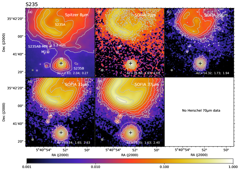
Figure 1: Multi-wavelength images of S235 with facility and wavelength given in the upper right corner of each panel. Contour level information is given in the lower right: lowest contour level in number of $\sigma$ above the background noise and corresponding value in mJy per square arcsec; then step size between each contour in log₁₀ mJy per square arcsec, then peak flux in Jy per square arcsec. The color map indicates the relative flux intensity compared to that of the peak flux in each image panel. The pink dashed circle shown in (e) denotes the aperture used for the fiducial photometry. Gray circles in the lower left show the resolution of each image. The black cross in all panels denotes the position of the radio source VLA-2 of Felli et al. (2006) at R.A.(J2000) = 05^h40^m52$\fs$40, Decl.(J2000) = $+$35$\arcdeg$41$\arcmin$30$\arcsec$. The triangle sign marks the position of the 1.2 mm core. The small white cross marks the position of S235AB-MIR. The $\times$ sign marks the position of the NIR K-band source M1 as well as VLA-1.

Estimates of the distance to the S235 A-B region vary from 1.6 - 2.5 kpc (e.g., Israel & Felli 1978; Burns et al. 2015). We adopt 1.8 kpc, following Evans & Blair (1981), Dewangan et al. (2016) and Shimoikura et al. (2016). High-resolution mm line and continuum and radio continuum observations towards S235 A-B were reported by Felli et al. (2004, 2006). Shimoikura et al. (2016) carried out observations of C¹⁸O emission toward S235 A-B and revealed that the clump has an elliptical shape, with a mass of $\sim 1000\>M_{\odot}$ and an average radius of $\sim 0.5\>$pc. Two compact HII regions, called S235 A and S235 B (e.g., Felli et al. 1997; Klein et al. 2005; Saito et al. 2007) are located in this clump, along with a mm continuum core with HCO⁺(1-0) outflows in-between, which is thought to be an embedded, earlier-stage YSO (Felli et al. 2004). The mm core has a MIR counterpart S235 AB-MIR and several water masers and methanol masers nearby (Kurtz et al. 2004). From their estimate of a luminosity of $\sim 10^{3}L_{\odot}$ of the source, Felli et al. (2004) suggested that S235 AB-MIR is an intermediate-mass YSO driving the molecular outflows and supplying the energy for the -60 km s^-1 water maser nearby. On the other hand, Dewangan & Anandarao (2011) concluded from SED fitting that S235 AB-MIR is the most massive protostar in the region with $m_{*}\sim 11\>M_{\odot}$ and still actively accreting and so not yet able to excite an HII region. However, they were cautious about the reliability of these results due to the limited number of data points (three in the MIR from IRAC bands and two in the sub-mm-continuum from Felli et al. 2004).

Another NIR K-band source with the largest infrared excess, M1, is reported to be associated with the radio source VLA-1 by Felli et al. (2006) and they suggested that it could be a B2-B3 star with an UCHII region, while Dewangan & Anandarao et al. (2011) suggested that it is a low-mass star, relatively young in its evolution. Both S235 AB-MIR (counterpart of the 1.2mm core) and M1 can be seen in our SOFIA images in Figure 1. However, due to their weak MIR emission, we do not focus on them in this paper.

Our analysis is focussed on the MIR source S235 B, which is associated with the radio source VLA-2 (Felli et al. 2006). S235 B is the brightest object in the S235 A-B cluster in all broad-bands from U to K, and thus may be a massive YSO (Boley et al. 2009). Krassner et al. (1982) detected hydrogen recombination lines and polycyclic aromatic hydrocarbon (PAH) emission features at 3.3, 8.7 and 11.3 $\mu$m. However, no 3.3 mm or 1.2 mm continuum or molecular lines are detected associated with S235 B (Felli et al. 2004). While there is large-scale ¹²CO, ¹³CO and C¹⁸O emission in the whole S235 region (Shimoikura et al. 2016; Dewangan & Ojha 2017), smaller-scale outflows specifically associated with S235 B have not yet been reported. For example, even in the high-resolution HCO⁺(1-0) map of Felli et al. (2004), whose field of view covers S235 B, there is no sign of HCO⁺(1-0) outflows emerging from S235 B. Boley et al. (2009) classified the central star of S235 B as an early-type (B1V) Herbig Be star surrounded by an accretion disk based on its spectrum from 3800-7200 Å, its location in a region of active star formation, the presence of the nearby nebulosity, the Balmer emission lines in the stellar spectrum, and the large H-K excess. Furthermore, its spectrum shows that the S235 B nebulosity is reflective in nature, with the central YSO in S235 B as the illuminating source. Given the mass inferred from the spectral type ($>10M_{\odot}$), Boley et al. suggested S235 B is likely to already be on the main sequence.

In our SOFIA images as shown in Figure 1, S235 B is much brighter than S235 AB-MIR and M1. The weak second component to the north of the radio source in the Spitzer 8 $\mu$m image is likely to be produced by a ghosting effect of the primary source, since it is not seen in the other IRAC images, the SOFIA images or the UKIDSS JHK band images.

4.1.2 IRAS 22198+6336

IRAS 22198+6336 was previously considered to be a massive YSO (Palla et al. 1991; Molinari et al. 1996; Sánchez-Monge et al. 2008) until an accurate distance of 764 $\pm$ 27 pc was derived from the parallax measurements of 22 GHz associated water masers (Hirota et al. 2008). These authors, after reanalyzing the protostellar SED, then proposed IRAS 22198+6336 is an intermediate-mass deeply embedded YSO with spectral type of late-B, equivalent to a Class 0 object in low-mass star formation. Sánchez-Monge et al. (2010) detected a compact source at 3.5, 2.7, and 1.3 mm coincident with the centimeter source reported by Sánchez-Monge et al. (2008) and surrounded by a faint structure extended toward the southwest. The high rotational temperature (100-150 K) derived from CH₃CN and CH₃OH, together with the chemically rich spectrum, is clear evidence that IRAS 22198 is an intermediate-mass hot core. The CO(1-0) emission in Sánchez-Monge et al. (2010) reveals an outflow with a quadrupolar morphology clearly centered on the position of the main dust condensation. Observations of the high-velocity emission of different outflow tracers HCO⁺(1-0), HCN(1-0) and SiO(2-1) seem to favor the superposition of two bipolar outflows. Higher angular resolution observations at 1.3 mm by Palau et al. (2013) reveal a counterpart of the cm source (MM2 in their nomenclature) and a faint extension to its south (MM2-S). Palau et al. suggest that MM2 is likely driving the southwest-northeast outflow, while an unresolved close companion of MM2 or MM2-S, which is only detected at 3.6$\mu$m, could be the driving source of the northwest-southeast outflow. Periodic flares of the 6.7-GHz methanol maser have been detected in IRAS 22198 and their characteristics can be explained by a colliding-wind binary model (Fujisawa et al. 2014).

Our SOFIA images reveal the MIR counterpart of the centimeter/millimeter source. Extended emission is seen towards the blue-shifted outflow in the southwest at 19 and 31 $\mu$m. In contrast, the extended emission at $\mu$m directly points to the south. Faint extended emission is also seen along the axes of the two outflows at 70 $\mu$m.

4.1.3 NGC 2071

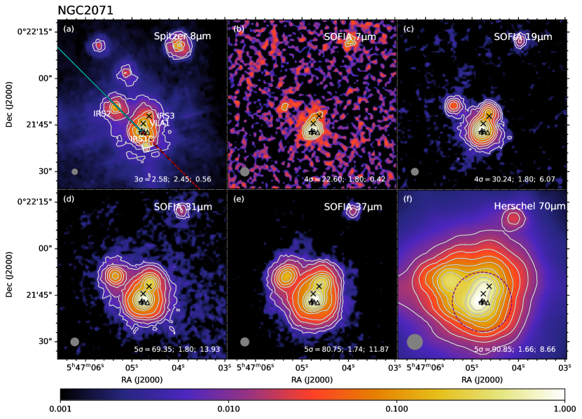
Figure 3: Multi-wavelength images of NGC 2071. The black cross in all panels denotes the position of the 1.3 cm source IRS 1C in Trinidad et al. (2009) at R.A.(J2000) = 05^h47^m04$\fs$741, Decl.(J2000) = $+$00$\arcdeg$21$\arcmin$42$\farcs$96. The $\times$ signs from north to south mark the positions of the 1.3 cm sources IRS3 and VLA1, respectively. The triangle signs from east to west mark the positions of the 1.3 cm sources IRS1E, IRS1W, and IRS1Wb, respectively. The lines in panel (a) show the orientation of the outflow axis (flow I), with the solid span tracing the blue-shifted direction and the dashed span the red-shifted direction. The outflow axis angle is from the high-velocity CO(1-0) main outflow emission of Stojimirović et al. (2008). Note that the center of the outflow has an uncertainty of $\sim$5″ and is not necessarily at IRS1C.

NGC 2071 is a reflection nebula located at a distance of 390 pc in the L1630 molecular cloud of Orion B (Anthony-Twarog 1982). The three brightest members of the infrared cluster at 10 $\mu$m, IRS1, IRS2 and IRS3, are each associated with compact radio sources at 5 GHz (Snell & Bally 1986). The radio continuum emission of IRS1 and IRS3 and the water masers associated with them suggest that both sources are associated with thermal jets (Smith & Beck 1994; Torrelles et al. 1998; Seth et al. 2002). Higher resolution VLA observations (Trinidad et al. 2009) break IRS1 into three continuum peaks (IRS1E, 1C and 1W), aligned in the east-west direction. Both the morphology and spectral index suggest that IRS1C is a thermal radio jet, while IRS1E and IRS1W could be condensations ejected by IRS1C. An energetic bipolar CO outflow has been observed toward NGC 2071, extending in the northeast-southwest direction and reaching $\sim$15’ in length (Bally 1982). In addition, shock-excited molecular hydrogen emission at 2.12 $\mu$m has also been reported showing a spatial extent similar to that of the CO outflow and revealing several H₂ outflows in the field, including one (flow II) perpendicular to the main outflow (flow I) (Eislöffel 2000). Stojimirović et al. (2008) also detected CO(1-0) emission in the direction of flow II. Trinidad et al. (2009) tried to identify individual driving sources for each outflow based on the observations of Eislöffel (2000) and the elongation of the IRS3 jet. However, we note that higher resolution observations of the outflows are needed to better distinguish the driving sources in this region.

Based on radio continuum emission indicating presence of thermal jets and water masers that are tracing disk-YSO-outflow systems, it has been proposed that IRS1 and IRS3 are intermediate- and low-mass YSOs, respectively (Smith & Beck 1994; Torrelles et al. 1998; Seth et al. 2002, Trinidad et al. 2009). In our SOFIA images, the three sources IRS1, IRS2 and IRS3 are revealed at all wavelengths (see Fig. 3). Here, we will focus on the SED of the IRS1 source, but the aperture we adopt also includes IRS3.

4.1.4 Cepheus E

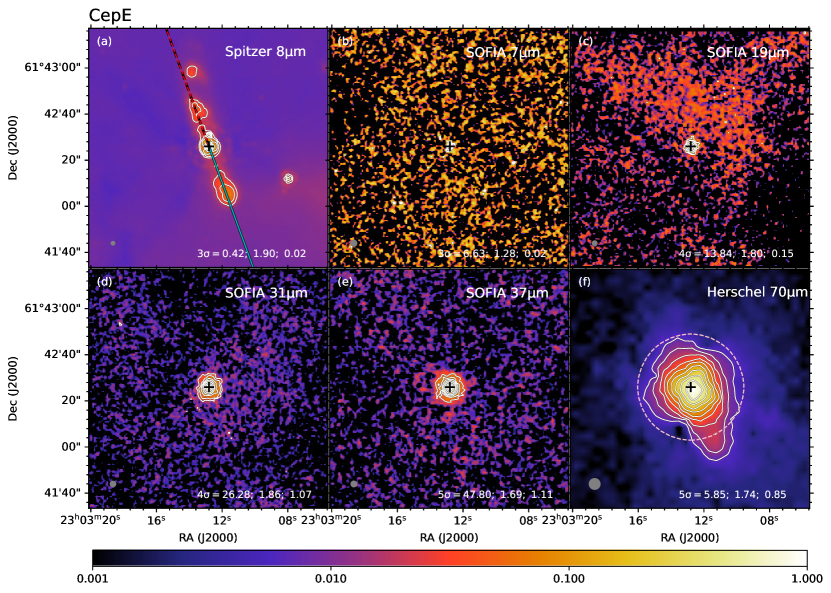
Figure 4: Multiwavelength images of Cep E. The black cross in all panels denotes the position of the 1.3 mm source CepE-A in Ospina-Zamudio et al. (2018) at R.A.(J2000) = 23^h03^m12$\fs$8, Decl.(J2000) = $+$61$\arcdeg$42$\arcmin$26$\arcsec$. The lines in panel (a) show the orientation of the outflow axis, with the solid span tracing the blue-shifted direction and the dashed span the red-shifted direction. The outflow axis angle is defined by the CO(2-1) outflow emission of Lefloch et al. (2015).

The Cepheus E (Cep E) molecular cloud is located at a distance of 730 pc (Sargent 1977). Since its early discovery by Wouterloot & Walmsley (1986) and Palla et al. (1993), subsequent studies have confirmed the central source Cep E-mm to be an isolated intermediate-mass protostar in the Class 0 stage (Lefloch et al. 1996; Moro-Martín et al. 2001). The source drives a very luminous molecular outflow and jet (Lefloch et al. 2011, 2015), terminated by the bright Herbig-Haro object HH377 in the south (Ayala et al. 2000). The 21″-long jet, the HH 377 terminal bow-shock, and the outflow cavity are clearly revealed in multiple CO transitions and the [OI] 63 $\mu$m line (Gusdorf et al. 2017). The observations are interpreted by means of time-dependent magneto-hydrodynamics (MHD) shock models by (Lefloch et al. 2015). Ospina-Zamudio et al. (2018) reveal Cep E-mm as a binary protostellar system with NOEMA observations. They identified two components from a two-component fit to the visibilities, Cep E-A and Cep E-B, which are separated by $\sim$ 1.7″. Ospina-Zamudio et al. argued Cep E-A dominates the core continuum emission and powers the well-known, high-velocity jet associated with HH 377, while the lower flux source Cep E-B powers another high-velocity molecular jet revealed in SiO(5-4) propagating in a direction close to perpendicular with respect to the Cep E-A jet. The spectra of molecular lines observed by NOEMA show bright emission of O- and N-bearing complex organic molecules (COMs) around Cep E-A and no COM emission towards Cep E-B.

From our SOFIA images (Fig. 4), we are not able to resolve the potential binary system, so our modeling will be an approximation of the properties of Cep E-A, assuming it dominates the system. The IR emission along the main jet is clearly seen in the Spitzer 8 $\mu$m image and also in the Herschel 70 $\mu$m image, since these space-based observations are more sensitive to fainter emission features.

4.1.5 L1206

Figure 5: Multi-wavelength images of L1206. The black crosses in all panels from east to west denote the position of the 8$\mu$m peak of L1206 B at R.A.(J2000) = 22^h28^m57$\fs$626, Decl.(J2000) = $+$64$\arcdeg$13$\arcmin$37$\farcs$348 and the position of L1206 A coincident with that of the 2.7 mm source OVRO 2 in Beltrán et al. (2006) at R.A.(J2000) = 22^h28^m51$\fs$41, Decl.(J2000) = $+$64$\arcdeg$13$\arcmin$41$\farcs$1, respectively. The lines in panel (a) show the orientation of the outflow axis from L1206 A, with the solid span tracing blue-shifted direction and the dashed span red-shifted direction. The outflow axis angle is given by the CO(1-0) outflow emission of Beltrán et al. (2006).

L1206, also known as IRAS 22272+6358, is located at a distance of 776 pc from the trigonometric parallaxes of 6.7 GHz methanol masers (Rygl et al. 2010). There are two MIR sources presented in our field of view. The western source IRAS 22272+6358 A (hereafter referred to as L1206 A) has no optical counterpart, and at near-infrared wavelengths, it has only been seen in scattered light (Ressler & Shure 1991). Given its extremely low 60/100 $\mu$m color temperature, L1206 A is believed to be very embedded, cold and young (Ressler & Shure 1991, Beltrán et al. 2006). It has been detected at 2.7 and 2 mm, but not at 2 or 6 cm (Wilking et al. 1989; McCutcheon et al. 1991; Sugitani et al. 2000; Beltrán et al. 2006). The 2.7 mm continuum observations by Beltrán et al. (2006) revealed four sources, OVRO 1, OVRO 2, OVRO 3, and OVRO 4, in a 12″ vicinity of L1206 A. The strongest millimeter source OVRO 2 is most likely the YSO associated with L1206 A, and is probably the driving source of the CO molecular outflow detected in the region. The dust emission morphology and properties of OVRO 2 suggest that this intermediate-mass protostar is probably in transition between Class 0 and I.

The K, L, L’ and M filter images of L1206 A reveal clearly lobes in a bipolar system (Ressler & Shure 1991). There is a distinct 3-4″ gap between the two lobes at the K, L, L’ bands. Since the proposed illuminating source lies within this gap, it is suggested by Ressler & Shure (1991) that this gap is produced by the extreme extinction of a thick, circumstellar disk. We also see such a gap in the 3.6, 4.5, and 5.8 $\mu$m images. The CO(1-0) observations of Beltrán et al. (2006) reveal a very collimated outflow driven by OVRO 2 with a very weak southeastern red lobe and a much stronger northwestern blue lobe. The relative brightness of the red lobe also decreases monotonically at K, L, L’ bands (Ressler & Shure 1991). Beltrán et al. (2006) suggested a scenario in which photodissociation produced by the ionization front coming from the bright-rimmed diffuse H II region in the south could be responsible for the weakness of the redshifted lobe and its overall morphology.

The elongation along the outflow direction of L1206 A is clearly revealed at 8 $mu$m. We see a slight extension along the outflow direction in our SOFIA images, especially at 31$\mu$m and 37 $\mu$m (see Fig. 5).

IRAS 22272 + 6358 B (hereafter referred to as L1206 B) is a bluer but less luminous object, which lies approximately 40″ to the east of L1206 A. Since L1206 B is directly visible at NIR and is likely to be a less obscured young stellar object, Ressler & Shure (1991) suggested that L1206 B is most likely a late Class I object or perhaps an early Class II object, whose photospheric spectrum is heavily extinguished by the parent cloud and is also affected by emission from a circumstellar disk.

From our SOFIA images, it can be seen that the emission of L1206 B becomes weaker as one goes to longer wavelengths, which also indicates that L1206 B may be more evolved than L1206 A.

4.1.6 IRAS 22172+5549

Figure 6: Multi-wavelength images of IRAS 22172. The black crosses in all panels from north to south denote the positions of the MIR peaks at 37$\mu$m MIR1 at R.A.(J2000) = 22^h19^m08$\fs$328, Decl.(J2000) = $+$56$\arcdeg$05$\arcmin$10$\farcs$522, MIR2 at R.A.(J2000) = 22^h19^m09$\fs$478, Decl.(J2000) = $+$56$\arcdeg$05$\arcmin$00$\farcs$370, and MIR3 at R.A.(J2000) = 22^h19^m09$\fs$430, Decl.(J2000) = $+$56$\arcdeg$04$\arcmin$45$\farcs$581, respectively. The white crosses from north to south mark the positions of the 1.3 mm sources MM1, MM4, MM2, MM3 in Palau et al. (2013) and the 3.4 mm source in Molinari et al. (2002) (also the mm core I22172-C in Fontani et al. 2004), respectively. The lines in panel (a) show the orientation of the outflow axis from MIR2, with the solid span tracing blue-shifted direction and the dashed span red-shifted direction. The outflow axis angle is from the CO(1-0) outflow emission of Fontani et al. (2004).

IRAS 22172+5549 is located at a kinematic distance of 2.4 kpc (Molinari et al. 2002). As a luminous IRAS source in the survey of Molinari et al. (2002), IRAS 22172 shows the presence of a compact dusty core without centimeter continuum emission, with prominent wings in the HCO⁺(1-0) line. Fontani et al. (2004) studied the 3 mm continuum and CO(1-0) emission in this region, finding a CO bipolar outflow centered at MIR2 (IRS1 in their nomenclature), which is offset by $\sim$ 7.5″ from the 3.4 mm peak. They suggested that the dusty core might host a source in a very early evolutionary stage prior to the formation of an outflow. From the outflow parameters, they proposed that MIR2, as the driving source, must be relatively massive. Palau et al. (2013) carried out higher angular resolution 1.3 mm and CO(2-1) observations. They detected more mm sources, including one confirmed protostar with no infrared emission that is driving a small outflow (MM2), two protostellar candidates detected only in the millimeter range (MM3 and MM4), and one protostellar object detected in the mm and infrared, with no outflow (MM1). MIR2 is still detected only in the infrared and is driving the larger CO(1-0) outflow. No mm emission or molecular outflows are detected towards MIR1 or MIR3. It is clear that IRAS 22172 harbors a rich variety of YSOs at different evolutionary stages.

Our SOFIA images (see Fig. 6) reveal extended emission along the blue-shifted outflow from MIR2, which could come from the outflow cavity.

4.1.7 IRAS 21391+5802

Figure 7: Multi-wavelength images of IRAS 21391. The black crosses in all panels from north to south denote the positions of the MIR source MIR-48 at R.A.(J2000) = 21^h40^m41$\fs$43, Decl.(J2000) = $+$58$\arcdeg$16$\arcmin$37$\farcs$8 in Choudhury et al. (2010) and 3.6 cm sources VLA2 at R.A.(J2000) = 21^h40^m41$\fs$90, Decl.(J2000) = $+$58$\arcdeg$16$\arcmin$12$\farcs$3 and VLA3 at R.A.(J2000) = 21^h40^m42$\fs$77, Decl.(J2000) = $+$58$\arcdeg$16$\arcmin$01$\farcs$3 in Beltrán et al. (2002). The white cross sign marks the position of the 3.6 cm source VLA1. The $\times$ signs from east to west mark the positions of the 3.1 mm sources BIMA3, BIMA2 and BIMA1, respectively. The lines in panel (a) show the orientation of the outflow axis from VLA2/BIMA2, with the solid span tracing blue-shifted direction and the dashed span red-shifted direction. The outflow axis angle is given by the high-velocity CO(1-0) main outflow emission of Beltrán et al. (2002).

IRAS 21391+5802 is deeply embedded in the bright-rimmed globule IC 1396N located at a distance of 750 pc (Matthews 1979). This region exhibits all of the signposts of an extremely young object, such as strong sub-mm and mm dust continuum emission (Wilking et al. 1993; Sugitani et al. 2000; Codella et al. 2001), line emission from high-density gas tracers (Serabyn et al. 1993; Cesaroni et al. 1999; Codella et al. 2001), and water maser emission (Felli et al. 1992; Tofani et al. 1995; Patel et al. 2000; Valdettaro et al. 2005). Sugitani et al. (1989) discovered an extended CO bipolar outflow, which was also mapped later by Codella et al. (2001). NIR images of the region have revealed a collimated 2.12$\mu$m H₂ jet driven by IRAS 21391 (Nisini et al. 2001, Beltrán et al. 2009). Based on mm observations, Beltrán et al. (2002) resolved IRAS 21391 into an intermediate-mass source named BIMA 2, surrounded by two less massive and smaller objects, BIMA 1 and BIMA 3. Choudhury et al. (2010) identified MIR-50 and 54 as the mid-infrared counterparts of BIMA 2 and BIMA 3 and did not detect any source associated with BIMA 1. The source located $\sim$ 25″ to the north of BIMA 2 was identified as MIR-48. BIMA 1, BIMA 2 and BIMA 3 are all associated with 3.6 cm continuum emission (Beltrán et al. 2002). Figure 7 shows the region as seen by Spitzer at 8 $\rm\mu m$ and by SOFIA-FORCAST. Our analysis focusses on the MIR-48, BIMA 2 and BIMA3 sources.

A strong CO(1-0) outflow along the east-west direction is centered at the position of BIMA 2, and another collimated, weaker, and smaller bipolar outflows elongated along the north-south direction are associated with BIMA 1, which is only detected at low velocities (see Figure 4 in Beltrán et al. 2002). At the position of MIR-48, we see weak, overlapping blue- and red-shifted CO(1-0) emission, which is also only detected at low velocities. There is no molecular emission detected towards BIMA 3. The east-west outflow driven by BIMA 2 is highly collimated, and the collimation remains even at low outflow velocities. Beltrán et al. (2002) interpreted the complex morphology of the outflows as being the result of the interaction of the high velocity gas with dense clumps surrounding the protostar. They also suggested that BIMA 2 fits very well correlations between source and outflow properties for low-mass Class 0 objects given by Bontemps et al. (1996).

Neri et al. (2007) used still higher angular resolution millimeter interferometric observations to reveal that BIMA 2 is a cluster of multiple compact sources with the primary source named IRAM 2A. The detection of warm CH₃CN in IRAM 2A implies that this is the most massive protostar and could be the driving source of this energetic outflow. This interpretation is also supported by the morphology of the 1.2 mm and 3.1 mm continuum emission, which are extended along the outflow axis tracing the warm walls of the biconical cavity (Fuente et al. 2009). The CH₃CN abundance towards IRAM 2A is similar to that found in low-mass hot corinos and lower than that expected towards IM and high mass hot cores. Based on the low CH₃CN abundance, Fuente et al. (2009) suggested that IRAM 2A is a low-mass or a Herbig Ae star instead of the precursor of a massive Be star, or alternatively, IRAM 2A is a Class 0/I transition object that has already formed a small photodissociation region (PDR).

For BIMA 1 and BIMA 3, Beltrán et al. (2002) suggested they are more evolved low-mass objects given their small dust emissivity index and the more compact appearance of their dust emission.

While extended morphologies of the three sources are revealed in our SOFIA images (see Fig. 7), the extension of BIMA 2 does not follow the northeast-southwest direction of the major outflow or the north-south direction of the weak, low-velocity outflow.

4.2 General Results from the SOFIA Imaging

Most of the sources presented in this paper are associated with outflows. In a few cases, such as IRAS 22198, L1206 A and IRAS 22172 MIR2, the SOFIA 20 to 40 $\mu$m images show modest extensions in the directions of the outflow axes, which was a common feature of the high-mass protostars in Papers I and II. However, the appearance of most of the IM protostars in the SOFIA images is quite compact, i.e., only a few beams across, and relatively round. In some of these cases, such as IRAS 22198, Cep E and IRAS 21391 (BIMA 2) Spitzer $8\>{\rm\mu m}$ images, which are sensitive to lower levels of diffuse emission, do reveal outflow axis elongation, which the SOFIA images are not able to detect. One contributing factor here is likely to be that the IM protostars are intrinsically less luminous than high-mass protostars and so produce less extended MIR emission. Another factor may be that the mass surface densities of their clump environments are lower than those of high-mass protostars (this is revealed in the derived values of $\Sigma_{\rm cl}$ from the SED fitting; see Section 4.3.2) and thus their MIR to FIR emission can appear more compact and more apparently symmetric. Three-color images of all the sources are presented together in Figure 8.

We notice that three of our sources are resolved into at least two components by higher angular resolution mm observations (within $\sim$ 0.01pc) including IRAS 22198, Cep E, IRAS 21391 BIMA2. A few mm sources are detected close to the main MIR source in IRAS 22172 located 3″- 8″(0.03 - 0.09 pc) away and a few mm sources are detected close to L1206 A located $\sim$ 12″(0.04 pc) away. Several jet-like condensations are revealed by radio observations in NGC 2071 IRS1 (within $\sim$ 0.01pc). This indicates that at least some of the protostars in our sample may have nearby companions.

From Figure 9, we see that three of the sources have high-resolution UKIDSS NIR imaging: S235, IRAS 22172 and IRAS 21391. These images show the presence of a number of NIR sources in the vicinities of the protostars, especially for S235 and IRAS 22172, which may be associated clusters of YSOs. On the other hand, IRAS 22198, NGC 2071, Cep E and L1206 appear more isolated in their NIR images, although is must be noted that these images have lower resolution and higher noise levels. We also note that S235 B is located (in projection) near the center of its cluster, while IRAS22172 MIR2 is closer to the eastern edge of its cluster.

Figure 8: Gallery of RGB images of the seven new regions analyzed in this paper, as labeled. The color intensity scales are stretched as arcsinh and show a dynamic range of 100 from the peak emission at each wavelength. The legend shows the wavelengths used and the beam sizes at these wavelengths. SOFIA-FORCAST 37 $\mu$m is shown in red. SOFIA-FORCAST 19 $\mu$m is shown in green. Spitzer 8 $\mu$m is shown in blue.

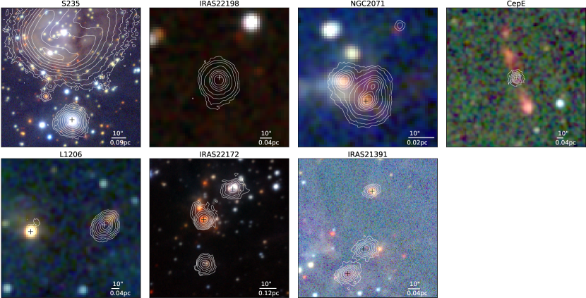
Figure 9: NIR RGB images of the seven new regions analyzed in this paper, as labeled. The data of S235, IRAS 22172 and IRAS 21391 are from the UKIDSS survey (Lawrence et al. 2007). The data of IRAS 22198, NGC 2071, Cep E and L1206 are from the 2MASS survey (Skrutskie et al. 2006). K band data are shown in red, H band data in green and J band data in blue. The white contours are the SOFIA 37$\mu$m emission, with the same levels as displayed in the previous individual figures for each source. The crosses in each panel are the same as those in the previous individual figures. The scale bar is shown in the right corner of each panel.

4.3 Results of SED Model Fitting

4.3.1 The SEDs

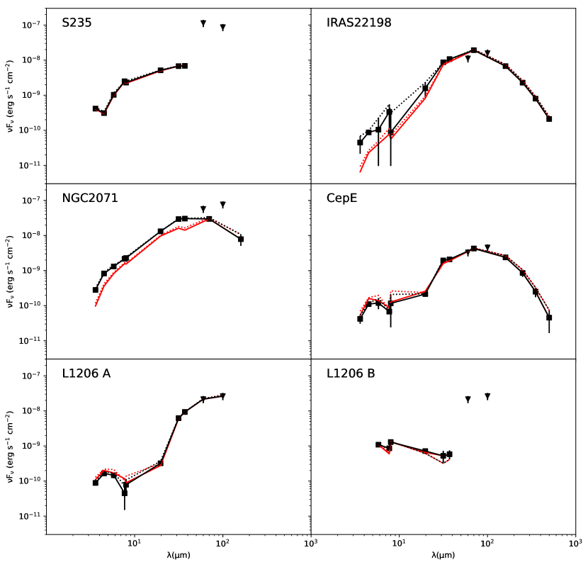
Figure 10: SEDs of the 14 presented sources. Total fluxes with no background subtraction applied are shown with dotted lines. The fixed aperture case is black dotted; the variable aperture (at $<70\>{\rm\mu m}$) case is red dotted. The background subtracted SEDs are shown with solid lines: black for fixed aperture (the fiducial case); red for variable aperture. Black solid squares indicate the actual measured values that sample the fiducial SED. Black triangles denote the flux densities measured with IRAS. The down arrows in G305 A and IRAS16562 N denote that those data points are fluxes with no background subtraction and are treated as upper limits.

Figure 10: (cont.)

Figure 10 shows the SEDs of the 14 sources presented in this paper. There are 10 sources that lack Herschel 70 and 160 $\mu$m observations, which makes it difficult to determine the location of the peak of their SEDs. For the remaining 4 sources, NGC 2071 has a SED that peaks between 37 and 70 $\mu$m, while IRAS 22198, Cep E and G305 A have their peaks around 70 $\mu$m. It is noticeable that L1206 B, IRAS22172 MIR2, IRAS22172 MIR1, IRAS21391 MIR48 and IRAS16562 N have very flat MIR SEDs, especially L1206 B even shows decreasing flux densities as the wavelength increases.

4.3.2 ZT Model Fitting Results

We now consider the results of fitting the ZT protostellar radiative transfer models to the SEDs. Note that a general comparison of differences in results when using the Robitaille et al. (2007) radiative transfer models was carried out in Paper I, with some of the main results being that the Robitaille et al. models often give solutions with very low accretion rates, which are not allowed in the context of the ZT models. As discussed in Paper I, our preference is to use the ZT models for analysis of the SOMA sources, since these models have been developed specifically for massive star formation under a physically self-consistent scenario, including full protostellar evolution, and with relatively few free parameters. Figure 11 shows the results of fitting the ZT protostellar radiative transfer models to the fixed aperture, background-subtracted SEDs, which is the fiducial analysis method presented in Papers I and II. In general, reasonable fits can be found to the observed SEDs, i.e., with relatively low values of reduced $\chi^{2}$.

A summary of fitted parameter results in the $\Sigma_{\rm cl}$ - $M_{c}$ - $m_{*}$ parameter space is shown for each source in Figure 12. Note that the clump environment mass surface density, $\Sigma_{\rm cl}$ (ranging from 0.1 to 3 $\rm g\>cm^{-2}$), and initial core mass, $M_{c}$ (ranging from 10 to 480 $M_{\odot}$), are the primary physical parameters of the initial conditions of the ZT models, while the current protostellar mass, $m_{*}$ (ranging from 0.5 $M_{\odot}$ up to about 50% of $M_{c}$, with this efficiency set by disk wind driven outflow feedback), describes the evolutionary state of stars forming from such cores. The two other independent parameters of the models are the angle of the line of sight to the outflow axis, $\theta_{\rm view}$, and the amount of foreground extinction, $A_{V}$, with all other model parameters being completely specified by $\Sigma_{\rm cl}$, $M_{c}$, and $m_{*}$. Note that $L_{\rm bol,iso}$ represents the isotropic bolometric luminosity, i.e., without correction for the inclination, and $L_{\rm bol}$ represents the intrinsic bolometric luminosity. The best five model fits for each source are listed in Table 4. Note that $\chi^{2}$ listed in this table is the reduced $\chi^{2}$, i.e., already normalized by the number of data points used in the fitting. Note, also that Table 4 of Paper II listed, incorrectly, this as quantity as $\chi^{2}/N$, rather than as $\chi^{2}$ used here and in Paper I.

The best-fit models indicate that S235 and G305 A are more likely to be high-mass protostars, with most of the models (except the best model for S235) returning protostellar masses $m_{*}\geq 12\>M_{\odot}$, accretion rates $\dot{m}_{*}\sim 10^{-5}-\rm a\ few\ \times 10^{-4}\>M_{\odot}\>{\rm yr}^{-1}$, initial core masses $M_{c}\sim 50-400\>M_{\odot}$, clump mass surface densities $\Sigma_{\rm cl}\sim 0.1-1\>\rm g\ cm^{-2}$, and isotropic luminosities $L_{\rm bol,iso}\sim 10^{3}-\rm a\ few\ \times 10^{4}\>L_{\odot}$.

We find that IRAS 22198, NGC 2071, L1206 A, L1206 B, IRAS22172 MIR2, IRAS22172 MIR3, IRAS21391 MIR48, and IRAS16562 N are likely to currently be intermediate-mass protostars, with most models returning protostellar masses $m_{*}\sim 2-8\ M_{\odot}$, accretion rates $\dot{m}_{*}\sim 10^{-5}-10^{-4}\>M_{\odot}\>{\rm yr}^{-1}$, initial core masses $M_{c}$ ranging from 10 to 480 $M_{\odot}$, clump mass surface densities $\Sigma_{\rm cl}$ ranging from 0.1 to 3.2 g cm^-2, and isotropic luminosities $L_{\rm bol,iso}\sim 10-\rm a\ few\ \times 10^{2}\>L_{\odot}$. However, given the estimated remaining envelope masses around these protostars, for many models the final outcome would be a massive star, since star formation efficiencies are typically $\sim 50\%$ in the models (see also Tanaka et al. 2017; Staff et al. 2019).

Considering the remaining sources, we see that Cep E, IRAS22172 MIR1, IRAS21391 BIMA2, IRAS21391 BIMA3 are likely to currently be low-mass protostars, with most models returning protostellar masses $m_{*}\sim 0.5-2\ M_{\odot}$, accretion rates $\dot{m}_{*}\sim 10^{-5}-10^{-4}\>M_{\odot}\>{\rm yr}^{-1}$, initial core masses $M_{c}$ ranging from 10 to 160 $M_{\odot}$, the clump mass surface densities $\Sigma_{\rm cl}$ ranging from 0.1 to 0.3 g cm^-2, and isotropic luminosities $L_{\rm bol,iso}\sim 10^{2}\>L_{\odot}$. Given that the models used for the fitting all have initial core masses of $10\>M_{\odot}$ or greater, then the outcome of the evolution would always be formation of at least intermediate-mass stars. However, within the degeneracies of the model fits, there are some solutions that would imply we are catching a massive star in the very earliest stages of its formation.

Below, we describe the fitting results of each individual source and compare then with previous estimates from the literature.

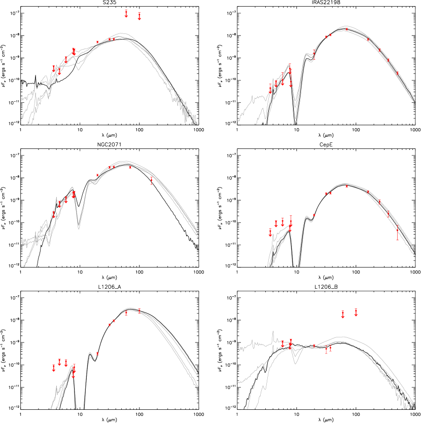
Figure 11: Protostar model fitting to the fixed aperture, background-subtracted SED data using the ZT model grid. For each source, the best fit model is shown with a solid black line and the next four best models are shown with solid gray lines. Flux values are those from Table 2. Note that the data at $\lesssim 8\>{\rm\mu m}$ are treated as upper limits (see text). The resulting model parameter results are listed in Table 4.

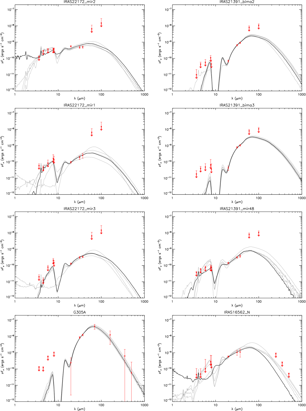
Figure 11: (cont.)

S235: From the best five model fits, this source has an estimated isotropic bolometric luminosity of $\sim 1$ to $2\times 10^{3}\>L_{\odot}$. However, the intrinsic bolometric luminosity of these models spans a much wider range from $3\times 10^{3}$ to $2\times 10^{5}\>L_{\odot}$. We note that for this source there are effectively only three measurements of the SED, all from the SOFIA FORCAST data, with observations at other wavelengths being used as upper limits. The large intrinsic luminosities for this source are possible because of the “flashlight effect”, i.e., most of the flux is not directed towards us due to high local extinction in the core. This range of intrinsic luminosities means that there is a wide range of protostellar properties that are consistent with the observed SED, i.e., there are significant degeneracies in the derived protostellar parameters (see Fig. 12). In particular, while the best fit model has a low initial core mass ($10\>M_{\odot}$) and current protostellar mass ($2\>M_{\odot}$) forming from a high $\Sigma_{\rm cl}$ environment ($3\>{\rm g\>cm}^{-2}$) that is viewed at a relatively small angle to the outflow axis, the next four best models are all with larger core and protostellar masses in lower density environments viewed at angles nearly orthogonal to the outflow axis, i.e., close to the equatorial plane where there would be the most line of sight extinction.

Among previous studies of S235, Felli et al. (2006) used JHK band images and MSX fluxes and derived a luminosity of $410L_{\odot}$, which they claimed must be considered to be a lower limit because the FIR part of the spectrum is not taken into account in their calculation. Dewangan & Anandarao (2011) used JHK band images and 2MASS and IRAC fluxes to do SED fitting with models from Robitaille et al. (2006, 2007). They derived $m_{*}\sim 6.5M_{\odot}$, $L_{\rm bol}\sim 575L_{\odot}$ and $M_{\rm env}\sim 9M_{\odot}$. The stellar source itself has been classified as a B1V star by Boley et al. (2009), with emission-line profiles indicative of an accretion disk. Based on the intensity of the reflected component, it was concluded that the accretion disk must be viewed nearly edge-on, which agrees with four of our best models and explains the discrepancy between $L_{\rm bol,iso}$ and $L_{\rm bol}$. Boley et al. (2009) estimated a mass accretion rate of $2-6\times 10^{-6}M_{\odot}\rm yr^{-1}$ for a B1V star with a mass of 13 $M_{\odot}$ using the Br$\gamma$ luminosity, which is comparable with the mass-loss rate of $4\times 10^{-6}M_{\odot}\rm yr^{-1}$ derived by Felli et al. (2006) from the radio flux density. However, our best models have disk accretion rates more than ten times higher. It should be noted that the accretion rate is not a free parameter in the ZT models and that the range of accretion rates is generally relatively high, being set by the properties of the initial cores and the mass surface density of their clump environments.

IRAS 22198: The best models are those with a protostar with current mass of 2 - 4 $M_{\odot}$, forming in a low mass surface density clump (0.1 - 0.3 $\rm g\ cm^{-2}$). Our estimate of the isotropic luminosity is about 600 $L_{\odot}$, with the intrinsic luminosity being about $800\>L_{\odot}$. Sánchez-Monge et al. (2010) fit the SED of IRAS 22198 from NIR to centimeter wavelengths with a modified blackbody plus a thermal ionized wind and derived a bolometric luminosity of $\sim$370 $L_{\odot}$ and an envelope mass of $\sim$5 $M_{\odot}$, remarking that the SED of IRAS 22198 resembles that of Class 0 objects (Andre et al. 1993). Our derived isotropic luminosity is slightly higher, while our envelope mass is much higher, $\sim 50\>M_{\odot}$, than their results. However, their $M_{\rm env}$ was derived from interferometric flux measurements and thus should be treated as a lower limit. The single-dish measurement at mm wavelengths of the dense core mass is 17 $M_{\odot}$ within a radius of 2,650 au (3.5″) (Palau et al. 2013). Thus the reason for our larger mass estimate is likely due to our analysis applying to a much larger scale, i.e., within a radius of 0.089 pc (26″).

NGC 2071: The best models suggest a currently intermediate-mass protostar with a mass of 2 - 4 $M_{\odot}$ forming within a core with initial mass of 10 - 60 $M_{\odot}$. Trinidad et al. (2009) estimated a central mass of $\sim 5\pm 3M_{\odot}$ for IRS1 and $\sim 1.2\pm 0.4M_{\odot}$ for IRS3 based on the observed velocity gradient of the water masers, which is consistent with our estimate. The single-dish measurement at mm wavelength of the dense core mass is 39 $M_{\odot}$ within a radius of 4,700 AU (11″) (Palau et al. 2013), which is similar to the $M_{\rm env}$ returned by most of our best fit models inside 10″.

Cep E: The best 5 models all return a $\Sigma_{\rm cl}$ of 0.1 $\rm g\ cm^{-2}$ and most models have $m_{*}$ as low as 1 - 2 $M_{\odot}$. Crimier et al. (2010) modeled the MIR to mm SED with the 1D radiative transfer code DUSTY and derived a luminosity of $\sim$100 $L_{\odot}$ and an envelope mass of 35 $M_{\odot}$, which are similar to our results.

L1206: The best models of L1206 A involve a protostar forming inside a relatively massive initial core (40 - 480 $M_{\odot}$) with low clump mass surface density (0.1 - 0.3 $\rm g\ cm^{-2}$). All the best 5 models give a value of $m_{*}=4\>M_{\odot}$. Ressler & Shure (1991) found a total luminosity of 1100 $L_{\odot}$ by fitting four IRAS fluxes plus the 2.7 mm data of Wilking et al. (1989) with a single-temperature dust spectrum at 1 kpc, which is similar to our result. Beltrán et al. (2006) estimated the core mass of OVRO 2 to be 14.2 $M_{\odot}$ from the 2.7 mm dust continuum emission at a distance of 910 pc. This core mass estimate is derived from interferometric observations that may be missing flux, and indeed three of our best-fit models give a much higher value of $M_{\rm env}$. Ressler & Shure (1991) suggested that L1206 A is seen only in scattered light because of heavy obscuration by an almost edge-on circumstellar disk. Four of the best five models return a nearly edge-on line of sight.

L1206 B has a very flat and slightly decreasing SED at short wavelengths. A circumstellar disk could explain the infrared excess, as suggested by Ressler & Shure (1991), and the protostar may have already cleared a significant portion of its envelope, thus explaining the decreasing spectrum between 10 and 30 $\mu$m. The favored ZT models have a wide range of stellar mass $m_{*}\sim 0.5-12\ M_{\odot}$, but low initial core mass $M_{\rm c}\sim 10-40\ M_{\odot}$, low current envelope mass of 1 to 9 $M_{\odot}$ and low mass surface density $\Sigma_{\rm cl}\sim 0.1-0.3\>\rm g\ cm^{-2}$ of the clump environment.

IRAS 22172: The models for the three MIR sources all involve protostars with masses $\sim$ 1 - 4 $M_{\odot}$ forming in relatively low-mass initial cores of 10 - 40 $M_{\odot}$. Fontani et al. (2004) divided the SED between the NIR cluster and the cold 3.4 mm core (their I22172-C) and performed two grey-body fits to the SED. The grey-body fit to the MSX and IRAS data with $\lambda\leqslant 25\mu$m, which represent the emission due to the cluster of stars surrounding the mm core I22172-C, yields a luminosity of $2.2\times 10^{2}\>L_{\odot}$. Based on the beam size and the MSX 21$\mu$m emission, their photometry should cover the whole field, i.e., all the three MIR sources. However, in our analysis we derive a much higher combined luminosity from the region, with contributions from the three MIR sources analyzed. The single-dish measurement at mm wavelengths of the dense core mass of MIR2 is 150 $M_{\odot}$ (Palau et al. 2013), much higher than the $M_{\rm env}$ given by our models. However, their core radius, represented by the deconvolved FWHM/2, is about 10″, while our mass estimate is based on an aperture radius of 4″.

IRAS 21391: Previous SED fitting with low-resolution data estimated the bolometric luminosity of IRAS 21391 to range from 235 $L_{\odot}$ (Saraceno et al. 1996) to 440 $L_{\odot}$ (Sugitani et al. 2000). Our fitting results for the three sources BIMA 2, BIMA 3 and MIR 48 all return isotropic luminosities $\lesssim$ 100 $L_{\odot}$. By using the relationship between the momentum rate and the bolometric luminosity (Cabrit & Bertout 1992), Beltrán et al. (2002) inferred a bolometric luminosity of 150 $L_{\odot}$ for BIMA 2.

Choudhury et al. (2010) fit the 1 - 24 $\mu$m SED derived from optical BVRI, Spitzer IRAC and MIPS observations with Robitaille et al. (2007) models and derived a luminosity of 197 $L_{\odot}$ and a stellar mass of 6 $M_{\odot}$ for BIMA 2 (their MIR-50), which are both higher than our results. As indicated by Figure 17, ZT models with $m_{*}$ higher than 5 $M_{\odot}$ have a very large $\chi^{2}$. The envelope mass of Choudhury et al. (2010) of 41 $M_{\odot}$ is also slightly higher than the $M_{c}$ and $M_{\rm env}$ in our first 3 best models. However, their disk accretion rate is about 1000 times lower than that in our best models, which is a known issue when comparing Robitaille et al. (2007) and ZT models (see discussion in De Buizer et al. 2017). Beltrán et al. (2002) estimated the circumstellar mass to be 5.1 $M_{\odot}$ based on BIMA 3.1 mm continuum observations, which should be treated as a lower limit of $M_{\rm env}$ given that it is an interferometric measurement subject to missing flux. Beltrán et al. (2002) suggested that the axis of the outflow should be close to the plane of the sky, given the morphology of the CO(1-0) outflows at low velocities with blue-shifted and redshifted gas in both lobes. However, in our best 5 models, only the third model has a more edge-on inclination.

Our best models for IRAS 21391 BIMA3 involve a protostar with a current stellar mass of 0.5 $M_{\odot}$ with a bolometric luminosity $\sim$ 100 $L_{\odot}$. The best-fit model in Choudhury et al. (2010) for BIMA 3 (their MIR-54) yields a luminosity of 33.4 $L_{\odot}$ and a stellar mass of 1.5 $M_{\odot}$. Beltrán et al. (2002) derived a circumstellar mass of 0.07 $M_{\odot}$ for BIMA 3, which is much lower than the predicted $M_{\rm env}$ by our best models.

Our best models for IRAS 21391 MIR48 involve a protostar with a mass ranging from 1 to 12 $M_{\odot}$. The best-fit model in Choudhury et al. (2010) for MIR-48 yields a luminosity of 280 $L_{\odot}$ and a stellar mass of 5 $M_{\odot}$, which is similar to the isotropic luminosity and the stellar mass in our best two models.

Table 4: Parameters of the Best Five Fitted Models

Source	$\chi^{2}$	$M_{\rm c}$	$\Sigma_{\rm cl}$	$R_{\rm core}$	$m_{*}$	$\theta_{\rm view}$	$A_{V}$	$M_{\rm env}$	$\theta_{w,\rm esc}$	$\dot{M}_{\rm disk}$	$L_{\rm bol,iso}$	$L_{\rm bol}$
		($M_{\odot}$)	(g $\rm cm^{-2}$)	(pc) ($\arcsec$)	($M_{\odot}$)	(°)	(mag)	($M_{\odot}$)	(deg)	($M_{\odot}$/yr)	($L_{\odot}$)	($L_{\odot}$)
S235	1.26	10	3.2	0.013 ( 2 )	2.0	39	0.0	6	35	1.8$\times 10^{-4}$	1.4$\times 10^{3}$	2.6$\times 10^{3}$
$d$ = 1.8 kpc	2.55	60	1.0	0.057 ( 7 )	24.0	89	11.1	5	71	1.9$\times 10^{-4}$	2.1$\times 10^{3}$	9.3$\times 10^{4}$
$R_{ap}$ = 12 ″	2.74	50	0.1	0.165 ( 19 )	12.0	89	4.0	15	59	3.4$\times 10^{-5}$	1.4$\times 10^{3}$	1.4$\times 10^{4}$
= 0.10 pc	3.00	80	1.0	0.066 ( 8 )	32.0	89	15.2	3	79	1.4$\times 10^{-4}$	1.6$\times 10^{3}$	1.6$\times 10^{5}$
	3.02	50	0.3	0.093 ( 11 )	16.0	80	0.0	8	68	7.1$\times 10^{-5}$	1.4$\times 10^{3}$	3.1$\times 10^{4}$
IRAS22198	0.18	80	0.1	0.208 ( 56 )	4.0	89	29.3	71	18	3.7$\times 10^{-5}$	6.0$\times 10^{2}$	8.5$\times 10^{2}$
$d$ = 0.8 kpc	0.27	60	0.1	0.180 ( 49 )	4.0	62	41.4	51	21	3.4$\times 10^{-5}$	6.1$\times 10^{2}$	8.9$\times 10^{2}$
$R_{ap}$ = 26 ″	1.08	100	0.1	0.233 ( 63 )	4.0	89	35.4	91	15	4.0$\times 10^{-5}$	6.5$\times 10^{2}$	8.8$\times 10^{2}$
= 0.09 pc	1.47	40	0.3	0.083 ( 22 )	2.0	22	9.1	35	17	5.3$\times 10^{-5}$	6.5$\times 10^{2}$	7.5$\times 10^{2}$
	1.78	50	0.1	0.165 ( 44 )	4.0	62	25.3	41	24	3.2$\times 10^{-5}$	5.1$\times 10^{2}$	7.9$\times 10^{2}$
NGC2071	3.14	10	3.2	0.013 ( 7 )	4.0	58	57.6	2	56	1.9$\times 10^{-4}$	5.0$\times 10^{2}$	1.9$\times 10^{3}$
$d$ = 0.4 kpc	3.59	30	0.1	0.127 ( 67 )	4.0	65	12.1	21	33	2.7$\times 10^{-5}$	3.6$\times 10^{2}$	7.7$\times 10^{2}$
$R_{ap}$ = 10 ″	5.79	40	0.1	0.147 ( 78 )	4.0	62	11.1	30	27	3.0$\times 10^{-5}$	4.4$\times 10^{2}$	7.5$\times 10^{2}$
= 0.02 pc	7.06	60	0.1	0.180 ( 95 )	2.0	29	0.0	55	15	2.5$\times 10^{-5}$	3.2$\times 10^{2}$	3.5$\times 10^{2}$
	7.57	50	0.1	0.165 ( 87 )	2.0	29	0.0	46	16	2.4$\times 10^{-5}$	2.8$\times 10^{2}$	3.1$\times 10^{2}$
CepE	0.63	30	0.1	0.127 ( 36 )	1.0	83	29.3	27	15	1.5$\times 10^{-5}$	1.3$\times 10^{2}$	1.7$\times 10^{2}$
$d$ = 0.7 kpc	0.70	30	0.1	0.127 ( 36 )	2.0	65	60.6	25	23	2.0$\times 10^{-5}$	1.5$\times 10^{2}$	2.4$\times 10^{2}$
$R_{ap}$ = 23 ″	0.80	40	0.1	0.147 ( 42 )	1.0	89	21.2	38	12	1.6$\times 10^{-5}$	1.3$\times 10^{2}$	1.7$\times 10^{2}$
= 0.08 pc	1.40	50	0.1	0.165 ( 46 )	1.0	89	19.2	48	11	1.7$\times 10^{-5}$	1.4$\times 10^{2}$	1.7$\times 10^{2}$
	1.67	20	0.1	0.104 ( 29 )	4.0	71	100.0	10	43	2.1$\times 10^{-5}$	1.9$\times 10^{2}$	6.8$\times 10^{2}$
L1206 A	0.08	480	0.1	0.510 ( 136 )	4.0	89	45.5	474	6	6.1$\times 10^{-5}$	9.2$\times 10^{2}$	1.0$\times 10^{3}$
$d$ = 0.8 kpc	0.09	400	0.1	0.465 ( 124 )	4.0	83	56.6	390	7	5.8$\times 10^{-5}$	9.4$\times 10^{2}$	1.0$\times 10^{3}$
$R_{ap}$ = 9 ″	0.17	50	0.3	0.093 ( 25 )	4.0	55	41.4	41	22	7.7$\times 10^{-5}$	8.8$\times 10^{2}$	1.4$\times 10^{3}$
= 0.03 pc	0.21	40	0.3	0.083 ( 22 )	4.0	89	28.3	31	25	7.2$\times 10^{-5}$	7.3$\times 10^{2}$	1.4$\times 10^{3}$
	0.23	240	0.1	0.360 ( 96 )	4.0	89	74.7	229	9	5.1$\times 10^{-5}$	9.0$\times 10^{2}$	1.0$\times 10^{3}$
L1206 B	0.13	40	0.1	0.147 ( 39 )	12.0	89	8.1	2	82	9.5$\times 10^{-6}$	5.7$\times 10^{1}$	1.1$\times 10^{4}$
$d$ = 0.8 kpc	0.45	30	0.3	0.072 ( 19 )	12.0	89	30.3	1	81	2.2$\times 10^{-5}$	7.0$\times 10^{1}$	1.2$\times 10^{4}$
$R_{ap}$ = 10 ″	0.55	10	0.3	0.041 ( 11 )	4.0	77	0.0	1	68	2.4$\times 10^{-5}$	4.9$\times 10^{1}$	6.7$\times 10^{2}$
= 0.04 pc	0.71	10	0.1	0.074 ( 20 )	2.0	51	0.0	4	50	1.1$\times 10^{-5}$	8.1$\times 10^{1}$	1.3$\times 10^{2}$
	2.26	10	0.1	0.074 ( 20 )	0.5	22	34.3	9	20	7.8$\times 10^{-6}$	1.5$\times 10^{2}$	7.5$\times 10^{1}$
IRAS22172 MIR2	1.67	40	0.1	0.147 ( 13 )	2.0	22	0.0	36	19	2.2$\times 10^{-5}$	3.9$\times 10^{2}$	2.7$\times 10^{2}$
$d$ = 2.4 kpc	2.27	30	0.1	0.127 ( 11 )	2.0	22	32.3	25	23	2.0$\times 10^{-5}$	8.0$\times 10^{2}$	2.4$\times 10^{2}$
$R_{ap}$ = 4 ″	2.39	20	0.1	0.104 ( 9 )	4.0	48	6.1	10	43	2.1$\times 10^{-5}$	3.4$\times 10^{2}$	6.8$\times 10^{2}$
= 0.04 pc	2.51	30	0.1	0.127 ( 11 )	1.0	13	37.4	27	15	1.5$\times 10^{-5}$	8.7$\times 10^{2}$	1.7$\times 10^{2}$
	2.81	10	1.0	0.023 ( 2 )	2.0	39	50.5	5	39	7.5$\times 10^{-5}$	1.0$\times 10^{3}$	7.6$\times 10^{2}$
IRAS22172 MIR1	0.04	20	0.1	0.104 ( 9 )	2.0	34	25.3	15	30	1.7$\times 10^{-5}$	1.4$\times 10^{2}$	1.9$\times 10^{2}$
$d$ = 2.4 kpc	0.04	20	0.1	0.104 ( 9 )	1.0	22	50.5	17	20	1.3$\times 10^{-5}$	2.7$\times 10^{2}$	1.5$\times 10^{2}$
$R_{ap}$ = 5 ″	0.20	10	3.2	0.013 ( 1 )	4.0	71	0.0	2	56	1.9$\times 10^{-4}$	1.9$\times 10^{2}$	1.9$\times 10^{3}$
= 0.05 pc	0.23	10	0.1	0.074 ( 6 )	1.0	34	1.0	7	31	1.0$\times 10^{-5}$	8.1$\times 10^{1}$	1.1$\times 10^{2}$
	0.40	30	0.1	0.127 ( 11 )	1.0	22	16.2	27	15	1.5$\times 10^{-5}$	1.7$\times 10^{2}$	1.7$\times 10^{2}$
IRAS22172 MIR3	0.19	30	0.1	0.127 ( 11 )	1.0	22	0.0	27	15	1.5$\times 10^{-5}$	1.7$\times 10^{2}$	1.7$\times 10^{2}$
$d$ = 2.4 kpc	0.39	30	0.1	0.127 ( 11 )	2.0	34	13.1	25	23	2.0$\times 10^{-5}$	1.9$\times 10^{2}$	2.4$\times 10^{2}$
$R_{ap}$ = 5 ″	0.45	10	3.2	0.013 ( 1 )	4.0	68	0.0	2	56	1.9$\times 10^{-4}$	2.1$\times 10^{2}$	1.9$\times 10^{3}$
= 0.05 pc	0.61	10	1.0	0.023 ( 2 )	4.0	68	0.0	1	59	7.7$\times 10^{-5}$	1.5$\times 10^{2}$	1.1$\times 10^{3}$
	0.97	20	0.1	0.104 ( 9 )	1.0	29	0.0	17	20	1.3$\times 10^{-5}$	1.2$\times 10^{2}$	1.5$\times 10^{2}$
IRAS21391 BIMA2	0.04	20	0.1	0.104 ( 29 )	0.5	34	74.7	19	13	9.6$\times 10^{-6}$	8.0$\times 10^{1}$	9.0$\times 10^{1}$
$d$ = 0.8 kpc	0.07	30	0.1	0.127 ( 35 )	0.5	22	74.7	29	10	1.1$\times 10^{-5}$	8.8$\times 10^{1}$	9.0$\times 10^{1}$
$R_{ap}$ = 8 ″	0.08	10	0.3	0.041 ( 11 )	2.0	71	19.2	5	43	3.0$\times 10^{-5}$	6.2$\times 10^{1}$	2.8$\times 10^{2}$
= 0.03 pc	0.14	40	0.1	0.147 ( 40 )	0.5	22	59.6	39	8	1.1$\times 10^{-5}$	8.7$\times 10^{1}$	8.8$\times 10^{1}$
	0.18	50	0.1	0.165 ( 45 )	0.5	22	48.5	49	7	1.2$\times 10^{-5}$	8.7$\times 10^{1}$	8.7$\times 10^{1}$
IRAS21391 BIMA3	0.18	80	0.1	0.208 ( 57 )	0.5	86	2.0	79	5	1.4$\times 10^{-5}$	8.6$\times 10^{1}$	9.2$\times 10^{1}$
$d$ = 0.8 kpc	0.20	100	0.1	0.233 ( 64 )	0.5	55	0.0	99	4	1.5$\times 10^{-5}$	8.9$\times 10^{1}$	9.1$\times 10^{1}$
$R_{ap}$ = 8 ″	0.23	60	0.1	0.180 ( 50 )	0.5	83	9.1	59	6	1.3$\times 10^{-5}$	8.0$\times 10^{1}$	8.7$\times 10^{1}$
= 0.03 pc	0.24	120	0.1	0.255 ( 70 )	0.5	22	0.0	118	4	1.5$\times 10^{-5}$	9.0$\times 10^{1}$	8.8$\times 10^{1}$
	0.26	160	0.1	0.294 ( 81 )	0.5	22	0.0	158	3	1.6$\times 10^{-5}$	1.0$\times 10^{2}$	9.8$\times 10^{1}$
IRAS21391 MIR48	0.33	10	0.3	0.041 ( 11 )	4.0	89	43.4	1	68	2.4$\times 10^{-5}$	2.9$\times 10^{1}$	6.7$\times 10^{2}$
$d$ = 0.8 kpc	0.58	10	0.1	0.074 ( 20 )	2.0	68	13.1	4	50	1.1$\times 10^{-5}$	2.5$\times 10^{1}$	1.3$\times 10^{2}$
$R_{ap}$ = 8 ″	2.70	40	0.1	0.147 ( 40 )	12.0	89	98.0	2	82	9.5$\times 10^{-6}$	5.7$\times 10^{1}$	1.1$\times 10^{4}$
= 0.03 pc	3.75	30	0.3	0.072 ( 20 )	12.0	89	100.0	1	81	2.2$\times 10^{-5}$	7.0$\times 10^{1}$	1.2$\times 10^{4}$
	5.51	10	0.1	0.074 ( 20 )	1.0	39	92.9	7	31	1.0$\times 10^{-5}$	6.4$\times 10^{1}$	1.1$\times 10^{2}$
G305 A	0.16	240	0.3	0.203 ( 10 )	12.0	83	85.9	216	15	2.0$\times 10^{-4}$	3.1$\times 10^{4}$	4.1$\times 10^{4}$
$d$ = 4.1 kpc	0.17	320	0.3	0.234 ( 12 )	12.0	71	79.8	293	13	2.2$\times 10^{-4}$	3.3$\times 10^{4}$	4.0$\times 10^{4}$
$R_{ap}$ = 12 ″	0.19	200	0.3	0.185 ( 9 )	12.0	80	81.8	173	17	1.9$\times 10^{-4}$	2.8$\times 10^{4}$	4.0$\times 10^{4}$
= 0.24 pc	0.20	200	0.3	0.185 ( 9 )	16.0	83	97.0	162	22	2.2$\times 10^{-4}$	3.0$\times 10^{4}$	5.3$\times 10^{4}$
	0.20	400	0.3	0.262 ( 13 )	12.0	22	90.9	373	11	2.3$\times 10^{-4}$	3.7$\times 10^{4}$	4.0$\times 10^{4}$
IRAS16562 N	0.05	10	3.2	0.013 ( 2 )	4.0	62	0.0	2	56	1.9$\times 10^{-4}$	2.9$\times 10^{2}$	1.9$\times 10^{3}$
$d$ = 1.7 kpc	0.14	50	0.1	0.165 ( 20 )	2.0	22	0.0	46	16	2.4$\times 10^{-5}$	3.1$\times 10^{2}$	3.1$\times 10^{2}$
$R_{ap}$ = 8 ″	0.28	10	1.0	0.023 ( 3 )	1.0	29	17.2	8	25	6.0$\times 10^{-5}$	5.6$\times 10^{2}$	7.7$\times 10^{2}$
= 0.06 pc	0.37	60	0.1	0.180 ( 22 )	2.0	22	0.0	55	15	2.5$\times 10^{-5}$	3.5$\times 10^{2}$	3.5$\times 10^{2}$
	0.38	30	0.1	0.127 ( 15 )	4.0	62	7.1	21	33	2.7$\times 10^{-5}$	3.8$\times 10^{2}$	7.7$\times 10^{2}$

G305 A: The best models are those with a high-mass protostar with a current mass of 12 - 16 $M_{\odot}$ forming from a core with initial mass of 200 - 400 $M_{\odot}$ and initial clump mass surface density of 0.3 g cm^-2. In Paper II we mentioned G305A is likely to be much younger and more embedded than G305B and in a hot core phase, prior to the onset of an UC H II region.

IRAS16562 N: The best models involve a low-mass protostar with current mass of 1 - 4 $M_{\odot}$ forming from a core with initial mass of 10 - 60 $M_{\odot}$. $\Sigma_{\rm cl}$ is not well constrained, varying from 0.1 to 3.2 g cm^-2.

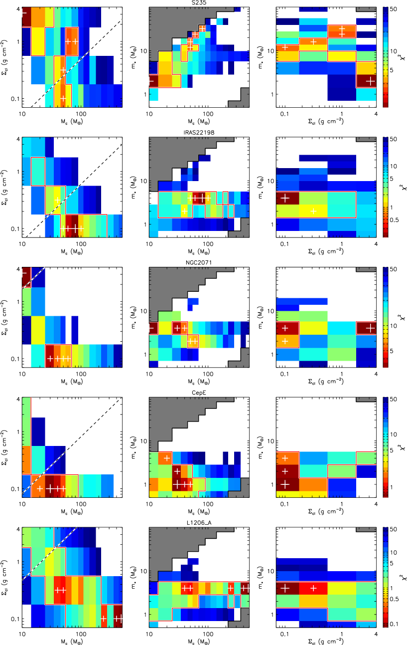
Figure 12: Diagrams of $\chi^{2}$ distribution in $\Sigma_{\rm cl}$ - $M_{c}$ space, $m_{*}$ - $M_{\rm c}$ space and $m_{*}$ - $\Sigma_{\rm cl}$ space. The white crosses mark the locations of the five best models, and the large cross is the best model. The grey regions are not covered by the model grid, and the white regions are where the $\chi^{2}$ is larger than 50. The red contours are at the level of $\chi^{2}$ = $\chi^{2}_{min}$ + 5. The dashed line denotes when $R_{c}=R_{\rm ap}$.

Figure 12: (cont.)

Figure 12: (cont.)

Figure 12 shows the $\chi^{2}$ distribution in $\Sigma_{\rm cl}$ - $M_{c}$ space, $m_{*}$ - $M_{c}$ space and $m_{*}$ - $\Sigma_{\rm cl}$ space for the 14 sources. As also discussed in Paper II, these diagrams illustrate the full constraints in the primary parameter space derived by fitting the SED data, and the possible degeneracies. In general, all the three parameters span a larger range compared with the sources of Papers I and II.

Follow-up observations and analysis of SOMA sources can be helpful in breaking degeneracies that arise from simple SED fitting. One example of such follow-up work is that of Rosero et al. (2019), who examined cm radio continuum data of the SOMA sources presented in Paper I. Radio free-free emission from photoionized gas, first expected to be present in the outflow cavity, is particularly useful for contraining the mass of the protostar once it reaches $\gtrsim 10\>M_{\odot}$ and begins to contract to the zero age main sequence. However, at lower masses most of the ionization associated with the source is expected to be due to shock ionization, e.g., due to internal shocks in the outflow (see also Fedriani et al. 2019). Quantitative models for the amount of shock ionization and associated radio emission have not yet been developed for the ZT protostellar models. For the mainly intermediate-mass sources presented in this paper, we anticipate that cm radio emission will main be due to shock ionization, so such observations may be more challenging to interpret to help break SED fit degeneracies. On the other hand, measurements of protostellar outflow properties, including cavity opening angle and mass and momentum fluxes may provide more diagnostic power.

In contrast with the high-mass protostars in Papers I and II, the best models ($\chi^{2}-\chi^{2}_{\rm min}<5$, within the red contours shown in Figure 12) of the intermediate-mass protostars also occupy the region with lower $M_{c}$ at lower $\Sigma_{\rm cl}$. Another striking feature is that most sources have best models with a core size larger than the aperture size, i.e., they appear below the dashed line denoting when $R_{c}=R_{\rm ap}$ in Figure 12. To examine this matter further, we analyzed the image profiles of the best 5 models of the sources and found that the flux density at 37 $\mu$m usually decays to $10^{-3}$ of the peak flux density within 5″ from the center and the flux density at 70 $\mu$m usually decays to $10^{-3}$ of the peak flux density within 15″ from the center. The typical aperture radius is $\sim$ 10″ (except for the three sources in IRAS 22172 where it is $\sim$ 5″, but their best models have the flux density decaying to $10^{-3}$ of the peak within 2″ and 5″ at 37 and 70 $\mu$m, respectively). This indicates that when the models have a core size larger than the aperture used for measuring the SED, only a small amount of the total flux from the model is being missed (however, the proportion of missed flux would be larger at longer wavelengths). Nevertheless, to better illustrate the importance of this effect, in the following discussion we present two cases, i.e., with and without the constraint on the model core size needing to be within a factor of two of the aperture size.

5 Discussion

We now discuss results of the global sample of 29 protostars that have been derived from an uniform SED fitting analysis that always includes SOFIA-FORCAST data, as presented in Papers I, II and III.

In general, we select the best five or fewer models that satisfy $\chi^{2}<\chi^{2}_{\rm min}+5$, where $\chi^{2}_{\rm min}$ is the value of $\chi^{2}$ of the best model, and then present averages of model properties. However, for G45.12+0.13, which was discussed in Paper II as not being especially well fit by the ZT models because of its high luminosity (it is likely to be multiple sources), there is only one model with $\chi^{2}<\chi^{2}_{\rm min}+5$. Thus for this source we average all the best 5 models. The model properties are averaged in log space, i.e., geometric averages, except for $A_{V}$, $\theta_{\rm view}$ and $\theta_{\rm w,esc}$, which are evaluated as arithmetic means.

Then, as explained at the end of the last section, we also consider two cases, i.e., without and with the constraint of “best-fit” models having core sizes that are within a factor of two of the aperture size. Without the core size constraint, the best five models of all sources automatically satisfy $\chi^{2}<\chi^{2}_{\rm min}+5$, except for G45.12+0.13. With the core size constraint (which we regard as our best, fiducial method), there can be cases, especially of intermediate-mass sources from Paper III (i.e., this work), where there are fewer than five models with $\chi^{2}<\chi^{2}_{\rm min}+5$. Still, G45.12+0.13 is kept as a special case, as above. Key average source properties are listed in Table 5.

5.1 The SOMA Sample Space

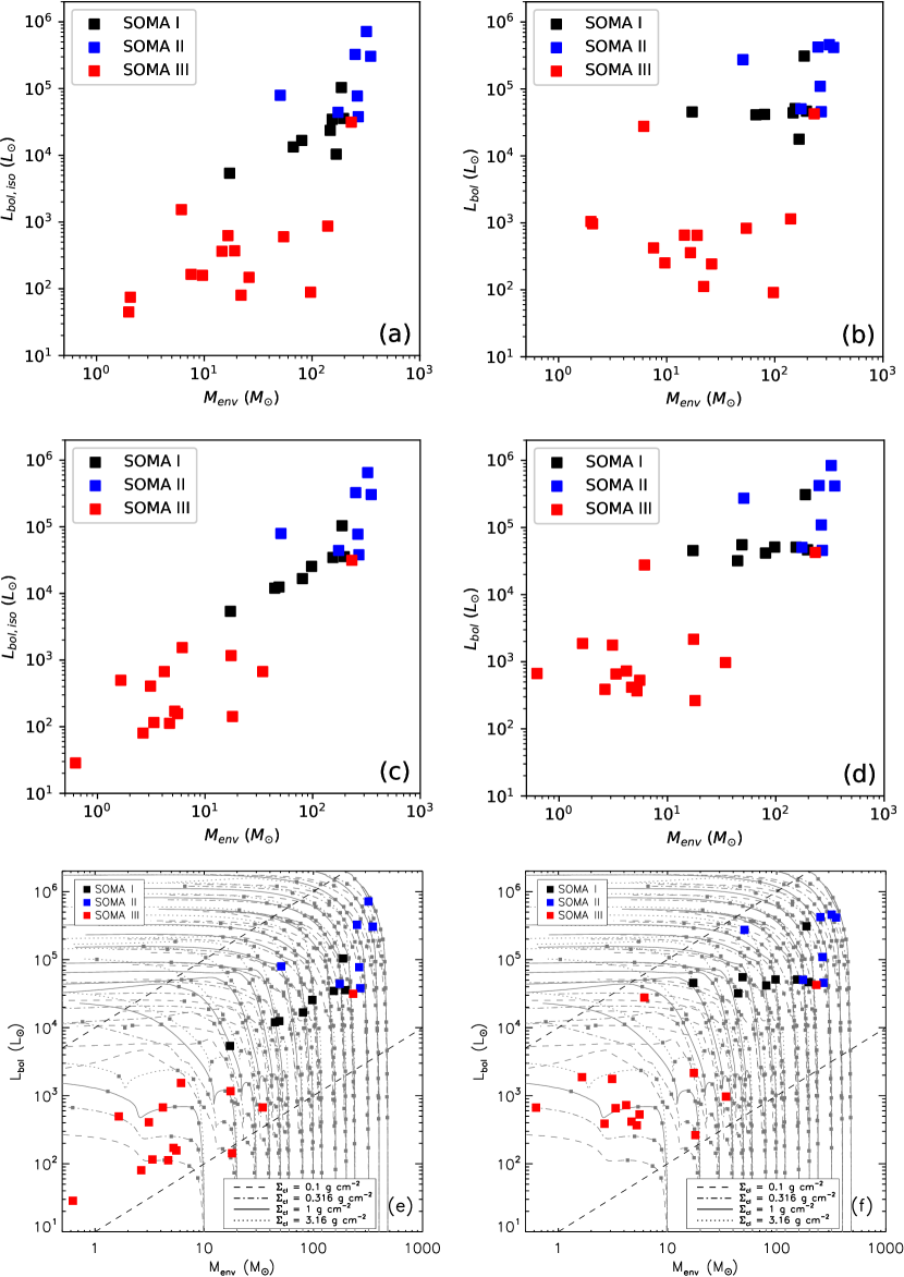
Figure 13: (a) Average (geometric mean) isotropic bolometric luminosity versus envelope mass returned by the best five (see text) ZT models for each SOMA source from Papers I, II and III (this work), as labelled. (b) Same as (a), but now with true bolometric luminosities plotted versus envelope mass. (c) Same as (a), but now using the average of the best five or fewer models with $R_{c}\lesssim 2R_{\rm ap}$ and $\chi^{2}<\chi^{2}_{\rm min}+5$. (d) Same as (c), but now with true bolometric luminosities plotted versus envelope mass. (e) Same as (c), but now also showing the ZT18 protostar models (grey squares), which are a collection of different evolutionary tracks (grey lines) for different initial core masses and clump mass surface densities (see legend). The two dashed black lines indicate $L_{\rm bol}/M_{\rm env}=10$ and $10^{4}\ L_{\odot}/M_{\odot}$, respectively. (f) Same as (e), but now with true bolometric luminosities plotted versus envelope mass.

Figure 13a shows $L_{\rm bol,iso}$ versus $M_{\rm env}$ for the SOMA protostar sample from Papers I, II and this work, i.e., Paper III. Figure 13b shows $L_{\rm bol}$ versus $M_{\rm env}$ of the same sample. This is the more fundamental property of the protstar, since $L_{\rm bol,iso}$ is affected by the orientation of protostellar geometry to our line of sight and the flashlight effect. Compared with the sources presented in Papers I and II, which were exclusively high-mass protostars, $L_{\rm bol,iso}$, $L_{\rm bol}$ and $M_{\rm env}$ all extend down to lower values. When we apply the constraint on model core sizes, i.e., radii of the models need to be no larger than twice the radius of the aperture used to define the SED, then we see from Figures 13c and d that there is an apparent tightening of the correlations between $L_{\rm bol,iso}$ or $L_{\rm bol}$ with $M_{\rm env}$. Note that the highest-mass, highest-luminosity YSOs usually have best models with $R_{c}\lesssim R_{\rm ap}$ and are thus less influenced by this constraint.

Figures 13e and f show the sample distribution in the context of the whole ZT model grid, where lines indicate evolutionary tracks, i.e., from low luminosity and high envelope mass to high luminosity and low envelope mass, for different clump environment mass surface densities, $\Sigma_{\rm cl}$.

The SOMA sample spans a relatively broad range of evolutionary stages with $L_{\rm bol}/M_{\rm env}$ extending from $\sim$ 10 $L_{\odot}/M_{\odot}$ up to almost $10^{4}\>L_{\odot}/M_{\odot}$, indicated by the dashed lines in Figure 13f. As a result of this broad range and given the even wider range that is expected from the theoretical models, we do not fit the observed $L_{\rm bol}$ versus $M_{\rm env}$ distribution with a power law relation (c.f., Molinari et al. 2008; Urquart et al. 2018). Rather, we simply note that the sources that have so far been analyzed in the SOMA sample span this wide range of evolutionary stages, but the expected very late stages and very early stages are not especially well represented.

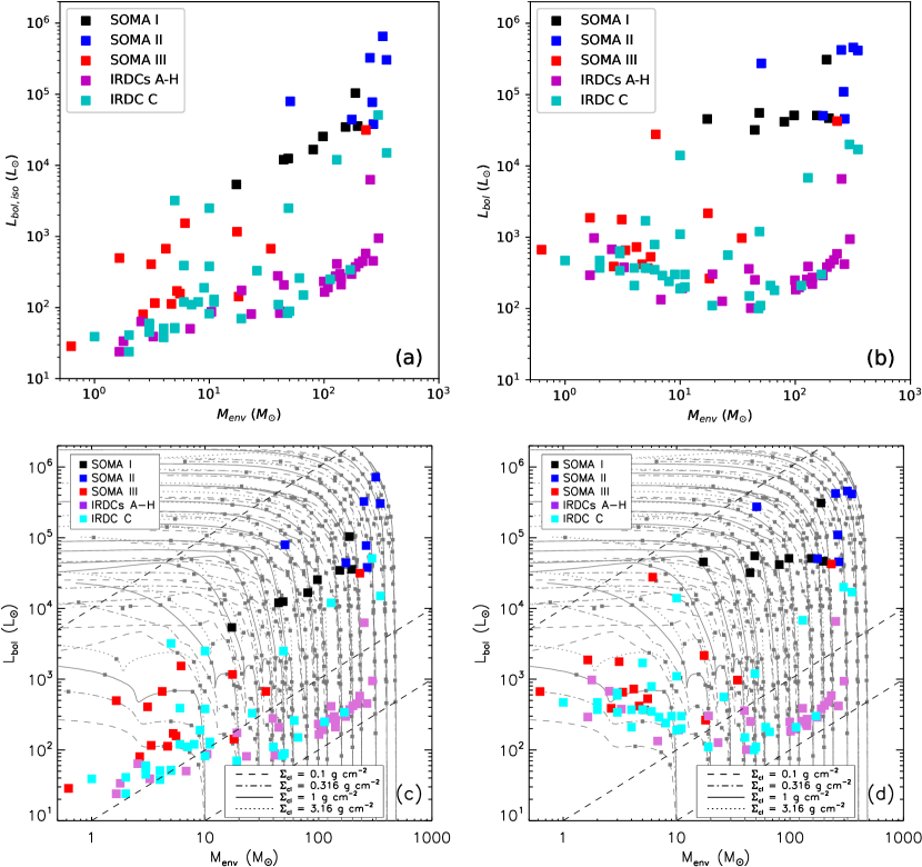
Figure 14: Protostellar evolutionary stages probed by the SOMA sample and IRDC protostar samples: “IRDC A-H” (Liu et al. 2018; Liu et al., in prep.); “IRDC C” (Moser et al. 2020). The format of the figures is otherwise the same as Figures 13c, d, e, f, respectively, but with the average (geometric mean) results of the valid models of IRDC sources added. The three dashed black lines in panels c and d indicate $L_{\rm bol}/M_{\rm env}=1,10$ and $10^{4}\ L_{\odot}/M_{\odot}$.

To further explore the evolutionary context of the SOMA protostars, in Figure 14 we show the SOMA sample in the luminosity versus envelope mass plane, together with protostellar sources identified in Infrared Dark Clouds (IRDCs), which are expected to be at earlier stages of evolution. Two samples of protostars selected from IRDC environments are shown, with the source SED construction and ZT model fitting following the same methods as have been used for the SOMA sample. The first, labelled “IRDCs A-H”, is the sample of 28 sources from Liu et al. (2018) and Liu et al., in prep., based on ALMA observations of 32 clumps in IRDCs A to H from the sample of Butler & Tan (2009, 2012). The second, labelled “IRDC C”, is a complete census of the protostellar sources in IRDC C carried out by Moser et al. (2020), based on sources identified in the region by Herschel 70 $\rm\mu m$ emission from the Hi-GAL point source catalog (Molinari et al. 2016). After allowing for a few poorly resolved sources that are treated as a single protostar in the SED modeling, a total of 35 protostars have been analyzed by Moser et al. (2020). The IRDC sources include protostars with intrinsic bolometric luminosities down to about $100\>L_{\odot}$, including within relatively massive core envelopes, so that the sampled values of $L_{\rm bol}/M_{\rm env}$ now extend down to $\sim 1\>L_{\odot}/M_{\odot}$.

Various biases in the input catalog for the SOMA survey likely account for the lack of sources at the final evolutionary stages of high $L_{\rm bol}$ and low $M_{\rm env}$. For example, these sources will have relatively weak MIR to FIR emission, which was used as a consideration to target SOMA protostars. Such sources may also be embedded within ultracompact H II regions, which we have tended to avoid, so far for analysis, even if they are within our fields of view: here the challenge is to isolate emission from any remaining protostellar core from the thermal emission from hot dust in the large scale H II region. Finally, this later phase of evolution may be relatively short, so objects here may be intrinsically rare. Future studies will attempt to identify such sources.

Finally, we note that a future goal is to extend complete surveys of high- and intermediate-mass protostars across their full range of evolutionary stages and across larger regions so that the samples can be used for demographic analyses that will inform about topics such as the duration of formation timescales. Previous work in this area, e.g., Davies et al. (2011), which covered large regions of the Galactic plane, focused only on high-mass protostars and have been relatively restricted in their coverage of earlier evolutionary stages.

5.2 The Shapes of SEDs

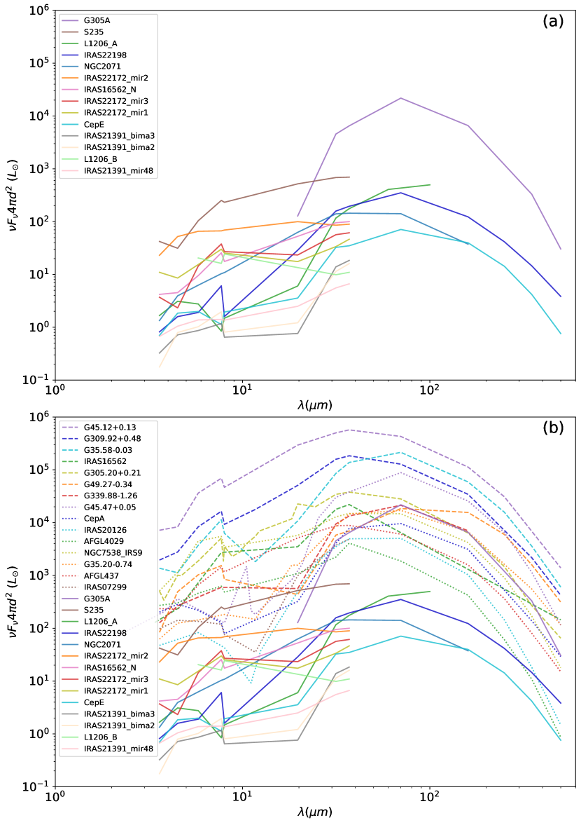
Figure 15: a) Top panel: Bolometric luminosity weighted SEDs of the 14 SOMA protostars analyzed in this paper. The ordering of the legend is from high to low ZT best fit model isotropic luminosity (top to bottom). b) Bottom panel: Same as (a), but now with addition of dashed lines denoting the sample of 15 sources from Papers I and II.

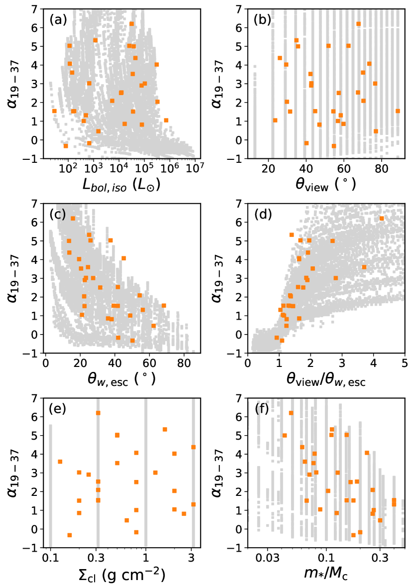
Figure 16: Spectral index, $\alpha_{19-37}$ between 19 $\mu$m and 37 $\mu$m (see text) versus: the geometric mean isotropic luminosity $L_{\rm bol,iso}$ (a: top left); the arithmetic mean inclination of viewing angle $\theta_{\rm view}$ (b: top right); the arithmetic mean opening angle $\theta_{w,\rm esc}$ (c: middle left); arithmetic mean $\theta_{\rm view}/\theta_{w,\rm esc}$ (d: middle right); the geometric mean clump surface density $\Sigma_{\rm cl}$ (e: bottom left); and geometric mean $m_{*}/M_{\rm c}$ (f: bottom right) returned by the best five or fewer models with $R_{c}\lesssim 2R_{\rm ap}$ and $\chi^{2}<\chi^{2}_{\rm min}+5$. The grey squares represents the ZT18 protostar models. Note that the spectral index of the models are calculated without foreground extinction and thus could be different from observations.

In Figure 15 we show the bolometric luminosity spectral energy distributions of the 14 protostars of this paper, together with the sample of 15 generally higher luminosity sources from Papers I and II. Here the $\nu F_{\nu}$ SEDs have been scaled by $4\pi d^{2}$ so that the height of the curves gives an indication of the luminosity of the sources assuming isotropic emission. The ordering of the vertical height of these distributions is largely consistent with the rank ordering of the predicted isotropic luminosity of the protostars from the best-fit ZT models (the legend in Figure 15 lists the sources in order of decreasing ZT best model isotropic luminosity).

We define a 19–37 $\mu$m spectral index via

$$\alpha_{19-37}=\frac{\nu_{37\mu m}F_{\nu,37\mu m}-\nu_{19\mu m}F_{\nu,19\mu m}}{\lambda_{37\mu m}-\lambda_{19\mu m}}.$$ (1)

In general, we expect that this index may vary systematically with protostellar source properties. Figure 16 shows the dependence of $\alpha_{19-37}$ of the SEDs on luminosity, inclination of viewing angle, outflow cavity opening angle, ratio of inclination of viewing angle to outflow cavity opening angle, $\Sigma_{\rm cl}$, and $m_{*}/M_{c}$, respectively. In all these panels, the results have been averaged over those of the best 5 or fewer models with core radii smaller than twice the aperture radius and $\chi^{2}<\chi^{2}_{\rm min}+5$ (except for G45.12+0.13, see above). We see that the outflow cavity opening angle has a strong influence on the 19–37 $\mu$m index, following the expectation that a relatively greater flux of shorter wavelength photons are able to escape from the protostellar core if the outflow cavity opening angle is larger. Also a viewing angle inclination that is relatively small compared to the outflow cavity opening angle will result in a flatter shorter wavelength SED, as also discussed in Paper II.

In Figure 16, we also plot the ZT18 models as grey squares beneath the observations to illustrate the model coverage. Note that the range shown here serves to best show the observations and does not represent the full parameter space of the ZT18 models. We note that while the observed correlations are in general built in the ZT models, the results of Figure 16 show how tight (or loose) the correlations are in practice of the observed SED spectral index in the SOFIA-FORCAST bands with best average protostellar parameters derived from the fitting the entire available MIR to FIR SED. This information gives an idea of how much information can be derived from only an observed value of $\alpha_{19-37}$.

Finally, and along the same lines, another important feature that is revealed by $\alpha_{19-37}$ is the protostellar evolutionary stage, as measured by $m_{*}/M_{c}$ (Figure 16f). Again, this general trend is expected in the context of the ZT models, since the outflow cavity systematically opens up during the course of the evolution and the envelope mass is depleted, resulting in lower overall extinction. There is also generally lower levels of extinction in protostellar cores in lower $\Sigma_{\rm cl}$ environments, but little correlation is seen here between $\alpha_{19-37}$ and $\Sigma_{\rm cl}$ (Figure 16e), indicating other factors have a more important influence.

5.3 Dependence of Massive Star Formation on Environment

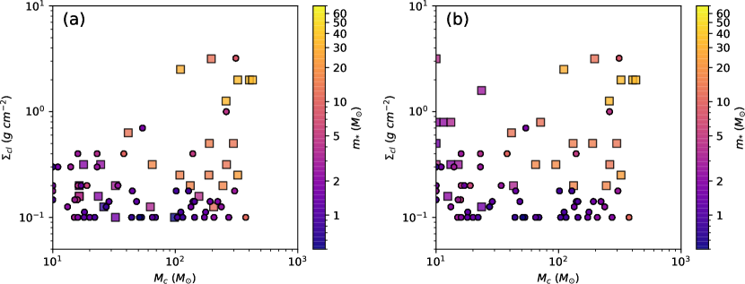
Figure 17: a) Left: Average clump mass surface density, $\Sigma_{\rm cl}$, versus average initial core mass, $M_{c}$, of the SOMA sources (squares) and IRDC sources (circles, Liu et al. 2018; Moser et al. 2020; Liu et al., in prep.), based on ZT model fits: the average is made for the best five selected models. b) Right: Same as (a), but with the average made for the best five or fewer models with $R_{c}\lesssim 2R_{\rm ap}$ and $\chi^{2}<\chi^{2}_{\rm min}+5$.

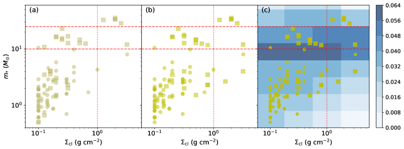
Figure 18: a) Left: Average protostellar mass, $m_{*}$, versus average clump mass surface density, $\Sigma_{\rm cl}$, of SOMA sources (squares) and IRDC sources (circles, Liu et al. 2018; Moser et al. 2020; Liu et al., in prep.), based on ZT model fits: the average is made for the best five selected models. The red dotted and dashed lines indicate fiducial threshold values of $m_{*}$ (10 and 25$\>M_{\odot}$) and $\Sigma_{\rm cl}$ (1$\>{\rm g\>cm}^{-2}$, see text). b) Middle: Same as (a), but with the average made for best five or fewer models with $R_{c}\lesssim 2R_{\rm ap}$ and $\chi^{2}<\chi^{2}_{\rm min}+5$. c) Right: Same as (b), but now also showing the distribution of models in the ZT model grid (shading indicates the density of models).

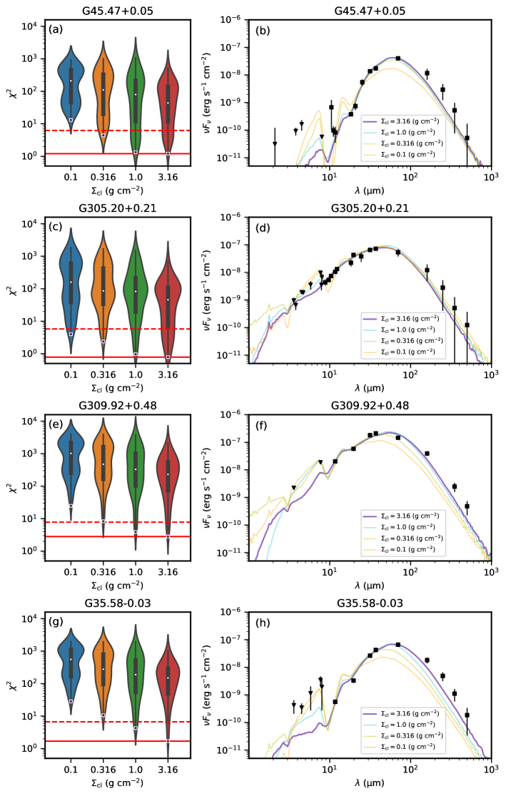
Figure 19: Left column: Violin plots of $\chi^{2}$ versus $\Sigma_{\rm cl}$ of all the models for several of the most massive protostars: G45.47+0.05, G305.20+0.21, G309.92+0.48 and G35.58-0.03. For the violin of each $\Sigma_{\rm cl}$, the white dot denotes the median $\chi^{2}$. The black bar in the center of the violin denotes the interquartile range (IQR). The black lines stretched from the bar denote the lower/upper adjacent values – defined as the furthest observation within 1.5 IQR of the lower/upper end of the bar. The width of the violin represents the probability density of the data value smoothed by a kernel density estimator. The squares at the bottom of each violin denote the smallest $\chi^{2}$ achieved by that $\Sigma_{\rm cl}$. The red solid line denotes $\chi^{2}_{\rm min}$ for the source. The red dashed line denotes $\chi^{2}_{\rm min}+5$. Right column: SEDs of the best model of each $\Sigma_{\rm cl}$ for each source (thickest line is the overall best model). The black triangles and squares with error bars denote the observations.

Figure 20: Star formation efficiency as a function of clump mass surface density, $\Sigma_{\rm cl}$, from model calculations of Tanaka et al. (2017). Models for initial core masses of $M_{c}=30,~{}100$, and $300{\rm\>M_{\odot}}$ are shown, as labelled.

Figure 21: a) Top Left: Average protostellar isotropic bolometric luminosity, $L_{\rm bol,iso}$, versus average clump mass surface density, $\Sigma_{\rm cl}$, of SOMA sources (squares) and IRDC sources (circles, Liu et al. 2018; Moser et al. 2020; Liu et al., in prep.), based on ZT model fits: the average is made for the best five selected models. b) Top Middle: Same as (a), but with the average made for best five or fewer models with $R_{c}\lesssim 2R_{\rm ap}$ and $\chi^{2}<\chi^{2}_{\rm min}+5$. c) Top Right: Same as (b), but now also showing the distribution of models in the ZT model grid (shading indicates the density of models). d) Bottom Left: Same as (a), but now for intrinsic bolometric luminosity, $L_{\rm bol}$. e) Bottom Middle: Same as (b), but now for intrinsic bolometric luminosity, $L_{\rm bol}$. f) Bottom Right: Same as (c), but now for intrinsic bolometric luminosity, $L_{\rm bol}$.

Figure 17 shows the distribution of values of $M_{c}$ (i.e., initial core mass), $\Sigma_{\rm cl}$ and $m_{*}$ of the 29 sources of the SOMA sample to date. With no constraint on the model core size, there appears to be an absence of protostars with low $M_{c}$ in high $\Sigma_{\rm cl}$ environments. However, this feature is not seen after applying the core size constraint, which we regard as the best method. Thus, the SOMA sample appears to contain protostars that have a range of initial core masses that can be present in the full range of protocluster clump mass surface density environments. However, note that these properties of $M_{c}$ and $\Sigma_{\rm cl}$ are not measured directly, but are inferred from the SED fitting.

We next examine if current protostellar properties depend on protocluster clump environment mass surface density. Figure 18 shows $m_{*}$ versus $\Sigma_{\rm cl}$. Figure 18a, similar to the results shown in Figure 17a, appears to show a lack of lower-mass sources in high-$\Sigma_{\rm cl}$ environments. However, this changes once the core size versus SED aperture constraint is applied (Fig. 18b), so we do not consider this to be a real effect. From the data shown in Fig. 18b, one potential trend that we notice is a lack of highest mass ($m_{*}\gtrsim 25\>M_{\odot}$) protostars in lower mass surface density environments ($\Sigma_{\rm cl}\lesssim 1\>{\rm g\>cm}^{-2}$). All of the five protostars with $m_{*}>25\>M_{\odot}$ (G45.47+0.05, G45.12+0.13, G305.20+0.21, G309.92+0.48, G35.58-0.03) are inferred to be in $\Sigma_{\rm cl}>1\>{\rm g\>cm}^{-2}$ environments. In Fig. 18c, we see that this trend is not a direct result of ZT model parameter space sampling, with density of models in the grid shown by the blue shading. High $m_{*}$ protostars forming from cores in low $\Sigma_{\rm cl}$ environments are present among the ZT models. We note that these models include protostellar outflow feedback, which sets star formation efficiencies close to 50%, but do not include radiative feedback, which would reduce the efficiency (see below).

We further examine how low $\Sigma_{\rm cl}$ models fail for high $m_{*}$ sources in Figure 19. Here we exclude G45.12+0.13 because none of the models fit particularly well for this source (see Paper II). We can see that the median $\chi^{2}$ and the smallest $\chi^{2}$ achieved generally decrease with $\Sigma_{\rm cl}$. Compared with high $\Sigma_{\rm cl}$ models, low $\Sigma_{\rm cl}$ models usually have higher fluxes at shorter wavelengths, i.e., $\lesssim 8\mu$m. These can be higher than the observational upper limits, which leads to a significant penalty in the fitting. Low $\Sigma_{\rm cl}$ models also tend to have lower fluxes at longer wavelength, i.e., $\gtrsim 20\mu$m. Therefore, they deviate away from the shape of the observed SEDs. We also tried manually adjusting $A_{V}$ or $L_{\rm bol}$ of the low $\Sigma_{\rm cl}$ models (not shown here), but such changes do not lead to significant improvement in model SED shape in comparison to the data.

Thus, we conclude there is tentative evidence from the SOMA sample analyzed so far that the most massive protostars require their cores to be in $\Sigma_{\rm cl}>1\ {\rm g\>cm}^{-2}$ environments, but larger further testing with a larger number of sources is clearly needed to confirm this.

Krumholz & McKee (2008) proposed that a minimum mass surface density of $1\>{\rm g\>cm}^{-2}$ is needed for massive star formation, based on protostellar heating suppression of fragmentation of massive cores by a population of surrounding lower-mass protostars (these protostars have higher accretion rates and thus luminosities in higher $\Sigma_{\rm cl}$ environments). While our result appears to confirm this prediction, we caution that the Krumholz & McKee model also predicts that $10\>M_{\odot}$ protostars would not be able to form in $\Sigma_{\rm cl}\lesssim 0.3\>{\rm g\>cm}^{-2}$ environments, which is inconsistent with the SOMA data. As an alternative, magnetic suppression of fragmentation to allow the existence of massive, early-stage cores has been discussed by, e.g., Butler & Tan (2012), with evidence of strong, $\sim 1$ mG $B$-fields inferred several cores in the IRDC 18310-4 region (Beuther et al. 2018).

The assembly of the highest mass pre-stellar cores, e.g., via a bottom-up process of merging smaller pre-stellar cores together or by general accumulation of clump gas, is expected to be more efficient in denser regions and this could provide an explanation, in the context of core accretion models, of the trends seen in Figure 18.

Once cores initiate star formation, then their accretion rates would also be higher in high surface density environments and this is expected to allow higher protostellar masses to be formed. Tanaka et al. (2017) assessed the expected star formation efficiency from cores due to both radiative and mechamical (i.e., outflow) feedback as a function of $\Sigma_{\rm cl}$ and found it can decrease by more than a factor of two for a given initial core as $\Sigma_{\rm cl}$ decreases from 3.2 to 0.1 $\rm g\>cm^{-2}$ (see Figure 20). The decrease is greatest for more massive cores, since once they start forming stars with $m_{*}\gtrsim 20\>M_{\odot}$, radiative feedback becomes powerful enough to truncate further accretion. For example, the $\Sigma_{\rm cl}=0.1\>{\rm g\>cm^{-2}}$ models shown in Figure 20 reach $m_{*}\simeq 10\>M_{\odot}$ starting from a $30\>M_{\odot}$ core, $m_{*}\simeq 20\>M_{\odot}$ starting from a $100\>M_{\odot}$ core, and $m_{*}\simeq 45\>M_{\odot}$ starting from a $300\>M_{\odot}$ core. However, the equivalent $\Sigma_{\rm cl}=1\>{\rm g\>cm^{-2}}$ models reach values of $m_{*}\simeq 15,40,$ and $100\>M_{\odot}$, respectively. Thus, in the context of these models, it is much more difficult to produce, e.g., $30\>M_{\odot}$ protostars in low-$\Sigma_{\rm cl}$ environments due to feedback effects, especially since the pre-stellar core mass function is expected to decline rapidly with increasing mass.

For competitive accretion models (Bonnell et al. 2001; Wang et al. 2010), higher mass surface density environments are also expected to lead to higher accretion rates and thus will probably also allow formation of higher-mass stars. However, the equivalent calculations for the effect of feedback have not yet been carried out for these models.

From an observational analysis of three clouds that are forming massive stars compared to several others that are not, Kauffmann et al. (2010) proposed a criterion for massive star formation equivalent to $\Sigma_{\rm cl}\geq 0.054(M_{\rm cl}/1000\>M_{\odot})^{-1/2}\>{\rm g\>cm}^{-2}$, which is relatively low compared to the thresholds discussed above. Also, this is a value smaller than the minimum of the range probed in the ZT18 protostellar model grid of $\Sigma_{\rm cl}=0.1g\>cm^{-2}$. Recently, Retes-Romero et al. (2020) studied 128 IRDCs to investigate if the Kauffmann et al. criterion predicts which of these IRDCs contains massive stars. They found that among the IRDCs satisfying this criterion, only one third of them currently contain massive YSOs. This may indicate that a higher, more localised value of $\Sigma_{\rm cl}$ is needed to form a massive star. For further progress on the general question of massive star formation thresholds, more direct measures of $\Sigma_{\rm cl}$, e.g., from dust continuum emission (in contrast to our indirect methods based on model fitting), on scales immediately surrounding the massive protostars and comparison to protostellar properties, e.g., as derived from SED fitting in the SOMA sample, are needed. However, such an analysis, which we defer to a future study, will inevitably be sensitive to how and where the protostellar core boundary is defined and such sensitivity will also need to be explored.

In summary, our results indicate, tentatively, that to form the most massive, $\gtrsim 25\>M_{\odot}$ protostars requires $\gtrsim 1\>{\rm g\>cm}^{-2}$ protocluster clump environments, although this is based on a relatively small number of (five) of protostellar sources that are in this mass range. We have a larger number (about 10) of protostars with $10\>M_{\odot}\lesssim m_{*}\lesssim 25\>M_{\odot}$ that are best fitted by models with $\Sigma_{\rm cl}\lesssim 0.3\>{\rm g\>cm^{-2}}$, so that there does not appear to be a particular mass surface density threshold, in this range, needed to form $10\>M_{\odot}$ protostars. These environmental dependencies on massive star formation need confirmation with larger numbers of sources. Such trends are consistent with several different theoretical expectations from core accretion models, including that due to decreasing star formation efficiency due to self-feedback for massive protostars in lower mass surface density environments.

Finally, we investigate the dependence of $L_{\rm bol,iso}$ and $L_{\rm bol}$ on $\Sigma_{\rm cl}$ in Figure 21. Once model core size to aperture constraints are applied (panels b and e), there is no strong correlation present in the overall distribution. The highest luminosity sources, which have the highest protostellar masses, are preferentially found in high mass surface density environments. This is not due to the sources having higher current accretion rates, since for these high $m_{*}$ sources, the accretion luminosity is only a relatively minor component of the total luminosity. Thus this trend is simply a reflection of those seen in the mass distribution of the sources.

Table 5: Average Parameters of SOMA Protostars

Source	$M_{\rm c}$	$\Sigma_{\rm cl}$	$m_{*}$	$m_{*}/M_{\rm c}$	$M_{\rm env}$	$L_{\rm bol,iso}$	$L_{\rm bol}$	$\theta_{\rm view}$	$\theta_{w,\rm esc}$	$\theta_{\rm view}/\theta_{w,\rm esc}$	$\alpha_{19-37}$
	($M_{\odot}$)	(g $\rm cm^{-2}$)	($M_{\odot}$)		($M_{\odot}$)	($L_{\odot}$)	($L_{\odot}$)	($\arcdeg$)	($\arcdeg$)
G45.12+0.13	403	2.0	35.5	0.09	319	7.2e+05	4.6e+05	24	21	1.12	1.05
	403	2.0	35.5	0.09	319	7.2e+05	4.6e+05	24	21	1.12	1.05
G309.92+0.48	323	2.0	33.5	0.10	251	3.3e+05	4.2e+05	30	22	1.37	2.04
	323	2.0	33.5	0.10	251	3.3e+05	4.2e+05	30	22	1.37	2.04
G35.58-0.03	427	2.0	33.5	0.08	350	3.1e+05	4.2e+05	29	19	1.63	4.03
	427	2.0	33.5	0.08	350	3.1e+05	4.2e+05	29	19	1.63	4.03
IRAS16562	323	0.3	22.9	0.07	263	7.7e+04	1.1e+05	43	23	1.90	2.91
	323	0.3	22.9	0.07	263	7.7e+04	1.1e+05	43	23	1.90	2.91
G305.20+0.21	110	2.5	28.5	0.26	51	7.9e+04	2.7e+05	47	38	1.24	0.82
	110	2.5	28.5	0.26	51	7.9e+04	2.7e+05	47	38	1.24	0.82
G49.27-0.34	197	3.2	12.0	0.06	174	4.4e+04	5.1e+04	26	14	1.92	4.38
	197	3.2	12.0	0.06	174	4.4e+04	5.1e+04	26	14	1.92	4.38
G339.88-1.26	298	0.5	12.7	0.04	269	3.8e+04	4.6e+04	36	14	2.70	5.00
	298	0.5	12.7	0.04	269	3.8e+04	4.6e+04	36	14	2.70	5.00
G45.47+0.05	260	1.3	32.8	0.13	187	1.0e+05	3.1e+05	77	27	2.80	3.01
	260	1.3	32.8	0.13	187	1.0e+05	3.1e+05	77	27	2.80	3.01
CepA	188	0.3	14.6	0.08	148	2.4e+04	4.4e+04	62	24	3.05	5.03
	132	0.5	14.6	0.11	98	2.6e+04	5.1e+04	52	26	1.96	5.03
IRAS20126	109	0.3	15.5	0.14	67	1.3e+04	4.1e+04	67	35	2.14	2.54
	95	0.3	17.8	0.19	49	1.2e+04	5.5e+04	67	42	1.60	2.54
AFGL4029	65	0.3	16.8	0.26	17	5.4e+03	4.5e+04	70	54	1.35	2.09
	65	0.3	16.8	0.26	17	5.4e+03	4.5e+04	70	54	1.35	2.09
NGC7538_IRS9	245	0.2	16.4	0.07	196	3.6e+04	4.7e+04	31	22	1.44	1.52
	245	0.2	16.4	0.07	196	3.6e+04	4.7e+04	31	22	1.44	1.52
G35.20-0.74	190	0.5	14.6	0.08	154	3.5e+04	5.1e+04	42	20	2.07	3.53
	190	0.5	14.6	0.08	154	3.5e+04	5.1e+04	42	20	2.07	3.53
AFGL437	133	0.2	16.4	0.12	80	1.7e+04	4.2e+04	60	36	1.64	0.86
	133	0.2	16.4	0.12	80	1.7e+04	4.2e+04	60	36	1.64	0.86
IRAS07299	206	0.1	10.8	0.05	168	1.0e+04	1.8e+04	83	21	4.85	2.51
	71	0.8	11.7	0.16	44	1.2e+04	3.2e+04	57	32	1.77	2.51
S235	41	0.6	12.4	0.30	6	1.5e+03	2.8e+04	77	62	1.23	0.46
	41	0.6	12.4	0.30	6	1.5e+03	2.8e+04	77	62	1.23	0.46
IRAS22198	63	0.1	3.5	0.06	55	6.0e+02	8.3e+02	65	19	3.52	3.03
	43	0.2	3.5	0.08	34	6.7e+02	9.7e+02	43	23	1.86	3.03
NGC2071	32	0.2	3.0	0.09	19	3.7e+02	6.5e+02	49	29	1.80	1.32
	10	3.2	4.0	0.40	2	5.0e+02	1.9e+03	58	56	1.04	1.32
CepE	32	0.1	1.5	0.05	26	1.5e+02	2.4e+02	79	21	5.05	3.60
	24	0.1	1.5	0.06	18	1.4e+02	2.6e+02	70	24	3.70	3.60
L1206_A	156	0.2	4.0	0.03	140	8.7e+02	1.1e+03	81	14	8.64	5.33
	24	1.6	2.6	0.11	17	1.2e+03	2.2e+03	35	25	1.40	5.33
L1206_B	16	0.2	3.6	0.22	2	7.5e+01	9.7e+02	66	60	1.09	-0.33
	12	0.2	2.2	0.17	3	8.0e+01	3.9e+02	55	50	1.09	-0.33
IRAS22172_mir2	24	0.2	2.0	0.09	17	6.3e+02	3.6e+02	29	28	1.02	-0.17
	11	0.8	2.3	0.20	4	6.7e+02	7.3e+02	40	42	0.92	-0.17
IRAS22172_mir3	18	0.3	2.0	0.11	8	1.6e+02	4.2e+02	44	35	1.35	1.53
	15	0.3	2.6	0.17	6	1.6e+02	5.3e+02	54	42	1.34	1.53
IRAS22172_mir1	16	0.2	1.5	0.09	10	1.6e+02	2.5e+02	37	31	1.22	1.54
	13	0.3	2.0	0.15	5	1.7e+02	3.7e+02	45	39	1.13	1.54
IRAS21391_bima2	26	0.1	0.7	0.03	22	8.0e+01	1.1e+02	34	16	2.52	4.07
	10	0.8	2.3	0.23	3	1.2e+02	6.6e+02	73	45	1.64	4.07
IRAS21391_bima3	98	0.1	0.5	0.01	97	8.9e+01	9.1e+01	54	5	11.10	5.03
	10	0.5	1.5	0.15	5	1.1e+02	4.2e+02	62	38	1.68	5.03
IRAS21391_mir48	16	0.2	4.1	0.25	2	4.5e+01	1.0e+03	75	63	1.22	1.54
	10	0.3	4.0	0.40	1	2.9e+01	6.7e+02	89	68	1.30	1.54
G305A	262	0.3	12.7	0.05	231	3.1e+04	4.3e+04	68	16	4.26	6.20
	262	0.3	12.7	0.05	231	3.1e+04	4.3e+04	68	16	4.26	6.20
IRAS16562_N	25	0.3	2.3	0.09	15	3.7e+02	6.5e+02	39	29	1.40	1.01
	13	0.8	3.5	0.26	3	4.1e+02	1.8e+03	57	49	1.15	1.01

Note. — The first line of each source shows the average (geometric mean, except for $\theta_{\rm view}$, $\theta_{\rm w,esc}$ and $\theta_{\rm view}/\theta_{w,\rm esc}$ for which arithmetic means are evaluated) of the values of the best five models without any core size versus aperture constraint applied. The second line shows the results of the best five or fewer models with $R_{c}\leq 2R_{\rm ap}$ and $\chi^{2}\leq\chi^{2}_{\rm min}+5$.

6 Conclusions

We have presented the results of MIR and FIR observations carried out towards 14 protostars in the SOMA survey, with most of them being intermediate-mass protostars. Following our standard methods developed in Papers I & II, we have built their SEDs with additional archival Spitzer, Herschel and IRAS data and fit them with Zhang & Tan (2018) RT models of massive star formation via the Turbulent Core Accretion paradigm. We have also supplemented the sample with protostars identified in Infrared Dark Clouds (IRDCs) and expected to be at very early stages in their evolution. By these methods we have extended the range of masses, luminosities and evolutionary stages of protostellar sources that have been analyzed in an uniform manner to test core accretion theory. Our main results and conclusions are:

1. The intermediate-mass protostars presented in this paper appear relatively compact at 20 – 40 $\mu$m, compared to the high-mass protostars in Papers I & II, whose 20 – 40 $\mu$m images more clearly show extension along their outflow axes. The protostars presented here are forming in a variety of protocluster environments, as revealed by NIR images. Higher resolution sub-mm images often reveal presence of secondary dense gas cores within 0.1 pc (in projection).

2. The SEDs of the 14 protostars of this paper are generally fit quite well by the ZT models, but there are significant degeneracies among acceptable models. These degeneracies in key model parameters, i.e., initial core mass, $M_{c}$, clump mass surface density, $\Sigma_{\rm cl}$, and current protostellar mass, $m_{*}$, are typically larger than for the higher mass protostars, but this is often a reflection of the more limited wavelength coverage of the intermediate-mass sources, which are often away from the Galactic plane and thus lacking, e.g., longer wavelength Herschel data. For the sources analyzed here, we find that well-fitting models can often have $R_{\rm c}>R_{\rm ap}$. Thus we have applied a further constraint that model core radii should not exceed the aperture radius used to define the SED by more than a factor of two.

3. The SOMA sources analyzed in this paper and Papers I & II span a range of bolometric luminosities of $\sim 10^{2}\>L_{\odot}$ to $\sim 10^{6}\>L_{\odot}$. The isotropic luminosity can be quite different from the intrinsic luminosity, indicating a significant flashlight effect in the sources.

4. The presented SOMA sample spans a range of light to mass ratios of $L_{\rm bol}/M_{\rm env}$ from $\sim 10\>L_{\odot}/M_{\odot}$ to $\sim 10^{4}\>L_{\odot}/M_{\odot}$. The addition of IRDC protostars extends this range down to $\sim 1\>L_{\odot}/M_{\odot}$, which is expected to be near the very earliest phases of the star formation process. Relatively late stages of evolution are currently missing from the sample.

5. The SED shape, as measured by the spectral index from 19 to 37 microns, shows trends with outflow opening angle, ratio of viewing angle to outflow opening angle, and evolutionary stage, i.e., $m_{*}/M_{c}$. However, such trends are features that are inherent in the ZT18 models and independent confirmation, e.g., from high resolution continuum and line studies of outflows and outflow cavities, is needed.

6. Protostars from low masses up to $\sim 25\>M_{\odot}$ are inferred to be forming at all the clump mass surface densities probed by the models, i.e., from 0.1 to 3 $\rm g\>cm^{-2}$. However, to form protostars with $>25\>M_{\odot}$ appears to require $\Sigma_{\rm cl}\gtrsim 1\>{\rm g\>cm}^{-2}$ clump environments. Larger numbers of sources in this mass range are needed to confirm this result. While this finding is consistent with several possible theoretical expectations, we favor one based on internal feedback in the protostellar core, which becomes less effective for the denser cores that are associated with higher $\Sigma_{\rm cl}$ environments (Tanaka et al. 2017).

References

- Andre et al. (1993) Andre, P., Ward-Thompson, D., & Barsony, M. 1993, ApJ, 406, 122
- Anthony-Twarog (1982) Anthony-Twarog, B. J. 1982, AJ, 87, 1213
- Ayala et al. (2000) Ayala, S., Noriega-Crespo, A., Garnavich, P. M., et al. 2000, AJ, 120, 909
- Bally (1982) Bally, J. 1982, ApJ, 261, 558
- Beltrán et al. (2002) Beltrán, M. T., Girart, J. M., Estalella, R., et al. 2002, ApJ, 573, 246
- Beltrán et al. (2006) Beltrán, M. T., Girart, J. M., & Estalella, R. 2006, A&A, 457, 865
- Beltrán et al. (2008) Beltrán, M. T., Estalella, R., Girart, J. M., et al. 2008, A&A, 481, 93
- Beltrán et al. (2009) Beltrán, M. T., Massi, F., López, R., et al. 2009, A&A, 504, 97
- Beltrán (2015) Beltrán, M. T. 2015, Ap&SS, 355, 283
- Beuther et al. (2018) Beuther, H., Soler, J. D., Vlemmings, W., et al. 2018, A&A, 614, A64
- Boley et al. (2009) Boley, P. A., Sobolev, A. M., Krushinsky, V. V., et al. 2009, MNRAS, 399, 778
- Bonnell et al. (2001) Bonnell, I. A., Bate, M. R., Clarke, C. J., & Pringle, J. E. 2001, MNRAS, 323, 785
- Bontemps et al. (1996) Bontemps, S., Andre, P., Terebey, S., et al. 1996, A&A, 311, 858
- Burns et al. (2015) Burns, R. A., Imai, H., Handa, T., et al. 2015, MNRAS, 453, 3163
- Butler & Tan (2009) Butler, M. J., & Tan, J. C. 2009, ApJ, 696, 484
- Butler, & Tan (2012) Butler, M. J., & Tan, J. C. 2012, ApJ, 754, 5.
- Cabrit & Bertout (1992) Cabrit, S., & Bertout, C. 1992, A&A, 261, 274
- Cesaroni et al. (1999) Cesaroni, R., Felli, M., & Walmsley, C. M. 1999, A&AS, 136, 333
- Choudhury et al. (2010) Choudhury, R., Mookerjea, B., & Bhatt, H. C. 2010, ApJ, 717, 1067
- Codella et al. (2001) Codella, C., Bachiller, R., Nisini, B., et al. 2001, A&A, 376, 271
- Crimier et al. (2010) Crimier, N., Ceccarelli, C., Alonso-Albi, T., et al. 2010, A&A, 516, A102
- Davies et al. (2011) Davies, B., Hoare, M. G., Lumsden, S. L., et al. 2011, MNRAS, 416, 972
- De Buizer et al. (2017) De Buizer, J. M., Liu, M., Tan, J. C., et al. 2017, ApJ, 843, 33
- Dewangan & Anandarao (2011) Dewangan, L. K., & Anandarao, B. G. 2011, MNRAS, 414, 1526
- Dewangan et al. (2016) Dewangan, L. K., Ojha, D. K., Luna, A., et al. 2016, ApJ, 819, 66
- Dewangan & Ojha (2017) Dewangan, L. K., & Ojha, D. K. 2017, ApJ, 849, 65
- Eislöffel (2000) Eislöffel, J. 2000, A&A, 354, 236
- Evans & Blair (1981) Evans, N. J., & Blair, G. N. 1981, ApJ, 246, 394
- Fazio et al. (2004) Fazio, G. G., Hora, J. L., Allen, L. E., et al. 2004, ApJS, 154, 10
- Fedriani et al. (2019) Fedriani, R., Caratti o Garatti, A., Purser, S. J. D., et al. 2019, Nature Communications, 10, 3630
- Felli et al. (1992) Felli, M., Palagi, F., & Tofani, G. 1992, A&A, 255, 293
- Felli et al. (1997) Felli, M., Testi, L., Valdettaro, R., et al. 1997, A&A, 320, 594
- Felli et al. (2004) Felli, M., Massi, F., Navarrini, A., et al. 2004, A&A, 420, 553
- Felli et al. (2006) Felli, M., Massi, F., Robberto, M., et al. 2006, A&A, 453, 911
- Fontani et al. (2004) Fontani, F., Cesaroni, R., Testi, L., et al. 2004, A&A, 424, 179
- Fuente et al. (2005) Fuente, A., Rizzo, J. R., Caselli, P., et al. 2005, A&A, 433, 535
- Fuente et al. (2009) Fuente, A., Castro-Carrizo, A., Alonso-Albi, T., et al. 2009, A&A, 507, 1475
- Fujisawa et al. (2014) Fujisawa, K., Takase, G., Kimura, S., et al. 2014, PASJ, 66, 78
- Griffin et al. (2010) Griffin, M. J., Abergel, A., Abreu, A., et al. 2010, A&A, 518, L3
- Gueth et al. (2001) Gueth, F., Schilke, P., & McCaughrean, M. J. 2001, A&A, 375, 1018
- Gusdorf et al. (2017) Gusdorf, A., Anderl, S., Lefloch, B., et al. 2017, A&A, 602, A8
- Hatchell et al. (2007) Hatchell, J., Fuller, G. A., & Richer, J. S. 2007, A&A, 472, 187
- Herter et al. (2013) Herter, T. L., Vacca, W. D., Adams, J. D., et al. 2013, PASP, 125, 1393
- Hirota et al. (2008) Hirota, T., Ando, K., Bushimata, T., et al. 2008, PASJ, 60, 961
- Israel & Felli (1978) Israel, F. P., & Felli, M. 1978, A&A, 63, 325
- Kauffmann et al. (2010) Kauffmann, J., Pillai, T., Shetty, R., et al. 2010, ApJ, 716, 433
- Klein et al. (2005) Klein, R., Posselt, B., Schreyer, K., et al. 2005, ApJS, 161, 361
- Krassner et al. (1982) Krassner, J., Pipher, J. L., Sharpless, S., et al. 1982, A&A, 109, 223
- Krumholz & McKee (2008) Krumholz, M. R., & McKee, C. F. 2008, Nature, 451, 1082
- Kurtz et al. (2004) Kurtz, S., Hofner, P., & Álvarez, C. V. 2004, ApJS, 155, 149
- Lawrence et al. (2007) Lawrence, A., Warren, S. J., Almaini, O., et al. 2007, MNRAS, 379, 1599.
- Lefloch et al. (1996) Lefloch, B., Eisloeffel, J., & Lazareff, B. 1996, A&A, 313, L17
- Lefloch et al. (2011) Lefloch, B., Cernicharo, J., Pacheco, S., et al. 2011, A&A, 527, L3
- Lefloch et al. (2015) Lefloch, B., Gusdorf, A., Codella, C., et al. 2015, A&A, 581, A4
- Liu et al. (2018) Liu, M., Tan, J. C., Cheng, Y., et al. 2018, ApJ, 862, 105
- Liu et al. (2019) Liu, M., Tan, J. C., De Buizer, J. M., et al. 2019, ApJ, 874, 16
- Matthews (1979) Matthews, H. I. 1979, A&A, 75, 345
- McCutcheon et al. (1991) McCutcheon, W. H., Dewdney, P. E., Purton, C. R., et al. 1991, AJ, 101, 1435
- McKee & Tan (2003) McKee, C. F., & Tan, J. C. 2003, ApJ, 585, 850
- Molinari et al. (1996) Molinari, S., Brand, J., Cesaroni, R., et al. 1996, A&A, 308, 573
- Molinari et al. (2002) Molinari, S., Testi, L., Rodríguez, L. F., et al. 2002, ApJ, 570, 758
- Molinari et al. (2008) Molinari, S., Pezzuto, S., Cesaroni, R., et al. 2008, A&A, 481, 345
- Molinari et al. (2016) Molinari, S., Schisano, E., Elia, D., et al. 2016, A&A, 591, A149
- Moro-Martín et al. (2001) Moro-Martín, A., Noriega-Crespo, A., Molinari, S., et al. 2001, ApJ, 555, 146
- Moser et al. (2020) Moser, E., Liu, M., Tan, J. C., et al. 2019, arXiv e-prints, arXiv:1907.12560, accepted to ApJ.
- Neri et al. (2007) Neri, R., Fuente, A., Ceccarelli, C., et al. 2007, A&A, 468, L33
- Neugebauer et al. (1984) Neugebauer, G., Habing, H. J., van Duinen, R., et al. 1984, ApJ, 278, L1
- Nisini et al. (2001) Nisini, B., Massi, F., Vitali, F., et al. 2001, A&A, 376, 553
- Ospina-Zamudio et al. (2018) Ospina-Zamudio, J., Lefloch, B., Ceccarelli, C., et al. 2018, A&A, 618, A145
- Palau et al. (2010) Palau, A., Sánchez-Monge, Á., Busquet, G., et al. 2010, A&A, 510, A5
- Palau et al. (2013) Palau, A., Fuente, A., Girart, J. M., et al. 2013, ApJ, 762, 120
- Palla & Stahler (1993) Palla, F., & Stahler, S. W. 1993, ApJ, 418, 414
- Palla et al. (1993) Palla, F., Cesaroni, R., Brand, J., et al. 1993, A&A, 280, 599
- Patel et al. (2000) Patel, N. A., Greenhill, L. J., Herrnstein, J., et al. 2000, ApJ, 538, 268
- Ressler & Shure (1991) Ressler, M. E., & Shure, M. 1991, AJ, 102, 1398
- Retes-Romero et al. (2020) Retes-Romero, R., Mayya, Y. D., Luna, A., et al. 2020, ApJ, 897, 53
- Robitaille et al. (2006) Robitaille, T. P., Whitney, B. A., Indebetouw, R., et al. 2006, ApJS, 167, 256
- Robitaille et al. (2007) Robitaille, T. P., Whitney, B. A., Indebetouw, R., et al. 2007, The Astrophysical Journal Supplement Series, 169, 328.
- Rosero et al. (2019) Rosero, V., Tanaka, K. E. I., Tan, J. C., et al. 2019, ApJ, 873, 20
- Rygl et al. (2010) Rygl, K. L. J., Brunthaler, A., Reid, M. J., et al. 2010, A&A, 511, A2
- Saito et al. (2007) Saito, H., Saito, M., Sunada, K., et al. 2007, ApJ, 659, 459
- Sánchez-Monge et al. (2008) Sánchez-Monge, Á., Palau, A., Estalella, R., et al. 2008, A&A, 485, 497
- Sánchez-Monge et al. (2010) Sánchez-Monge, Á., Palau, A., Estalella, R., et al. 2010, ApJ, 721, L107
- Saraceno et al. (1996) Saraceno, P., Ceccarelli, C., Clegg, P., et al. 1996, A&A, 315, L293
- Sargent (1977) Sargent, A. I. 1977, ApJ, 218, 736
- Serabyn et al. (1993) Serabyn, E., Guesten, R., & Mundy, L. 1993, ApJ, 404, 247
- Seth et al. (2002) Seth, A. C., Greenhill, L. J., & Holder, B. P. 2002, ApJ, 581, 325
- Shepherd & Watson (2002) Shepherd, D. S., & Watson, A. M. 2002, ApJ, 566, 966
- Shimoikura et al. (2016) Shimoikura, T., Dobashi, K., Matsumoto, T., et al. 2016, ApJ, 832, 205
- Skrutskie et al. (2006) Skrutskie, M. F., Cutri, R. M., Stiening, R., et al. 2006, AJ, 131, 1163
- Smith & Beck (1994) Smith, H. A., & Beck, S. C. 1994, ApJ, 420, 643
- Snell & Bally (1986) Snell, R. L., & Bally, J. 1986, ApJ, 303, 683
- Staff et al. (2019) Staff, J. E., Tanaka, K. E. I., & Tan, J. C. 2019, ApJ, 882, 123
- Stojimirović et al. (2008) Stojimirović, I., Snell, R. L., & Narayanan, G. 2008, ApJ, 679, 557
- Sugitani et al. (1989) Sugitani, K., Fukui, Y., Mizuni, A., et al. 1989, ApJ, 342, L87
- Sugitani et al. (2000) Sugitani, K., Matsuo, H., Nakano, M., et al. 2000, AJ, 119, 323
- Takahashi et al. (2012) Takahashi, S., Saigo, K., Ho, P. T. P., et al. 2012, ApJ, 752, 10
- Tanaka et al. (2017) Tanaka, K. E. I., Tan, J. C., & Zhang, Y. 2017, ApJ, 835, 32
- Tofani et al. (1995) Tofani, G., Felli, M., Taylor, G. B., et al. 1995, A&AS, 112, 299
- Torrelles et al. (1998) Torrelles, J. M., Gómez, J. F., Rodríguez, L. F., et al. 1998, ApJ, 505, 756
- Trinidad et al. (2009) Trinidad, M. A., Rodríguez, T., & Rodríguez, L. F. 2009, ApJ, 706, 244
- Urquhart et al. (2018) Urquhart, J. S., König, C., Giannetti, A., et al. 2018, MNRAS, 473, 1059
- Valdettaro et al. (2005) Valdettaro, R., Palla, F., Brand, J., et al. 2005, A&A, 443, 535
- van Kempen et al. (2012) van Kempen, T. A., Longmore, S. N., Johnstone, D., et al. 2012, ApJ, 751, 137
- Velusamy et al. (2011) Velusamy, T., Langer, W. D., Kumar, M. S. N., et al. 2011, ApJ, 741, 60
- Wang et al. (2010) Wang, P., Li, Z.-Y., Abel, T., & Nakamura, F. 2010, ApJ, 709, 27
- Wilking et al. (1989) Wilking, B. A., Mundy, L. G., Blackwell, J. H., et al. 1989, ApJ, 345, 257
- Wilking et al. (1993) Wilking, B., Mundy, L., McMullin, J., et al. 1993, AJ, 106, 250
- Wouterloot & Walmsley (1986) Wouterloot, J. G. A., & Walmsley, C. M. 1986, A&A, 168, 237
- Wu et al. (2004) Wu, Y., Wei, Y., Zhao, M., et al. 2004, A&A, 426, 503
- Young et al. (2012) Young, E. T., Herter, T. L., Güsten, R., et al. 2012, Proc. SPIE, 8444, 844410
- Zapata et al. (2007) Zapata, L. A., Ho, P. T. P., Rodríguez, L. F., et al. 2007, A&A, 471, L59
- Zhang, & Tan (2018) Zhang, Y., & Tan, J. C. 2018, ApJ, 853, 18