Revisiting Explicit Regularization in Neural Networks for Well-Calibrated Predictive Uncertainty

Abstract

From the statistical learning perspective, complexity control via explicit regularization is a necessity for improving the generalization of over-parameterized models. However, the impressive generalization performance of neural networks with only implicit regularization may be at odds with this conventional wisdom. In this work, we revisit the importance of explicit regularization for obtaining well-calibrated predictive uncertainty. Specifically, we introduce a probabilistic measure of calibration performance, which is lower bounded by the log-likelihood. We then explore explicit regularization techniques for improving the log-likelihood on unseen samples, which provides well-calibrated predictive uncertainty. Our findings present a new direction to improve the predictive probability quality of deterministic neural networks, which can be an efficient and scalable alternative to Bayesian neural networks and ensemble methods.

1 Introduction

As deep learning models have become pervasive in real-world decision-making systems, the importance of calibrated predictive uncertainty is increasing. The calibrated performance refers to the ability to match its predictive probability of an event to the long-term frequency of the event occurrence (Dawid, 1982). Well-calibrated predictive uncertainty is of interest in the machine learning community because it benefits many downstream tasks such as anomaly detection (Malinin & Gales, 2019), classification with rejection (Lakshminarayanan et al., 2017), and exploration in reinforcement learning (Gal & Ghahramani, 2016). Unfortunately, neural networks are prone to provide poorly calibrated predictions.

Bayesian neural networks have innate abilities to represent the model uncertainty. Specifically, they express the probability distribution over parameters, in which uncertainty in the parameter space is determined by the posterior inference (MacKay, 1992; Neal, 1993). Then, we can quantify predictive uncertainty from aggregated predictions from different parameter configurations. From this perspective, deterministic neural networks, which cannot provide such rich information, have been considered as lacking the uncertainty representation ability.

However, recent works (Lakshminarayanan et al., 2017; Müller et al., 2019; Thulasidasan et al., 2019) present a possibility of improving the quality of the predictive probability without changing the deterministic nature of neural networks. Specifically, they show that label smoothing (Szegedy et al., 2016), mixup (Zhang et al., 2018), and adversarial training (Goodfellow et al., 2015) significantly improve the calibration performance of neural networks. This direction is appealing because it can inherit the scalability, computational efficiency, and surprising generalization performance of the deterministic neural networks, for which Bayesian neural networks often struggle (Wu et al., 2019; Osawa et al., 2019; Joo et al., 2020a).

Motivated by these observations, we investigate a general direction from the regularization perspective to mitigate the poorly calibrated prediction problem. Specifically, we introduce a probabilistic measure of calibration performance, which is lower bounded by the log-likelihood. Based on this theoretical insight, we explore several explicit regularization methods for improving the log-likelihood on the test dataset, which leads to well-calibrated predictive uncertainty. Our extensive empirical evaluation shows that explicit regularization significantly improves the calibration performance of deterministic neural networks.

Our contributions can be summarized as follows: 1) our theoretical analysis clearly connects the log-likelihood with calibration performance, which provides a direction to improve the quality of predictive uncertainty. 2) we present a new direction for providing well-calibrated predictive uncertainty, which is readily applicable and computationally efficient; 3) our findings provide a novel view on the role and importance of explicit regularization in deep learning.

2 Background

We consider a classification problem with i.i.d. training samples $\mathcal{D}=\left\{({\bm{x}}^{(i)},y^{(i)})\right\}_{i=1}^{N}$ drawn from unknown distributions $P_{{\mathbf{x}},{\textnormal{y}}}$ whose corresponding tuple of random variables is $({\mathbf{x}},{\textnormal{y}})$. We denote $\mathcal{X}$ as an input space and $\mathcal{Y}$ as a set of class labels $\{1,2,\cdots,K\}$.

We define a classifier by a composition of a neural network and a softmax function; specifically, let $f^{{\bm{W}}}:\mathcal{X}\rightarrow\mathcal{Z}$ be a neural network with parameters ${\bm{W}}$ where $\mathcal{Z}=\mathbb{R}^{K}$ is a logit space. On top of the logit space, the softmax $\sigma:\mathbb{R}^{K}\rightarrow\triangle^{K-1}$ normalizes the exponential of logits:

$$\phi^{{\bm{W}}}_{k}({\bm{x}})=\frac{\exp(f^{{\bm{W}}}_{k}({\bm{x}}))}{\sum_{i}\exp(f^{{\bm{W}}}_{i}({\bm{x}}))}$$ (1)

where we let $\phi^{{\bm{W}}}_{k}({\bm{x}})=\sigma_{k}(f^{{\bm{W}}}({\bm{x}}))$ for brevity.

We often interpret $\phi^{{\bm{W}}}({\bm{x}})$ as the predictive probability that the label of ${\bm{x}}$ belongs to class $k$ (Bridle, 1990). Then, we train a neural network by maximizing the log-likelihood with stochastic gradient descent (SGD) (Robbins & Monro, 1951) or its variants. Here, we note a standard result that the maximum of the log-likelihood is achieved if and only if $\phi^{{\bm{W}}}({\mathbf{x}})$ perfectly matches $p({\textnormal{y}}|{\mathbf{x}})$.

2.1 Calibrated Predictive Uncertainty

A model with well-calibrated predictive uncertainty provides trustworthy predictive probability whose confidence aligns well with its expected accuracy. Formally, a well-calibrated model satisfies the following condition: $\forall{\bm{p}}\in\triangle^{K-1},k\in\{1,2,\cdots,K\},$

$$p({\textnormal{y}}=k|\phi^{{\bm{W}}}({\mathbf{x}})={\bm{p}})={\bm{p}}_{k}.$$ (2)

Here note that the calibrated model does not necessarily be ones achieving zero log-likelihood.

Given a finite dataset $\mathcal{D}$, we cannot evaluate the calibration condition in equation 2. Therefore, in practice, expected calibration error (ECE) (Naeini et al., 2015) is widely used as a calibration performance measure. ECE on $\mathcal{D}$ can be computed by binning predictions into $M$ groups based on their confidences and then averaging their calibration scores by:

$$\sum_{i=1}^{M}\frac{|\mathcal{G}_{i}|}{|\mathcal{D}|}|\text{acc}(\mathcal{G}_{i})-\text{conf}(\mathcal{G}_{i})|$$ (3)

where $\mathcal{G}_{i}=\left\{{\bm{x}}:\frac{i}{M}<\max_{k}\phi_{k}^{{\bm{W}}}({\bm{x}})\leq\frac{i+1}{M},{\bm{x}}\in\mathcal{D}\right\}$; $\text{acc}(\mathcal{G}_{i})$ and $\text{conf}(\mathcal{G}_{i})$ are average accuracy and confidence of predictions in group $\mathcal{G}_{i}$, respectively.

Another common way to evaluate the predictive uncertainty’s quality is based on predictive entropy, which assesses how well the model is aware of its ignorance. For example, predictive entropy is measured on misclassified or out-of-distribution (OOD) samples; that is, compute $-\sum_{k}\phi_{k}^{{\bm{W}}}({\bm{x}}^{\prime})\log\phi_{k}^{{\bm{W}}}({\bm{x}}^{\prime})$ for some ignorant sample ${\bm{x}}^{\prime}$. For a well-calibrated model, we expect the high predictive uncertainty on such samples, i.e., the answer “I don’t know.”

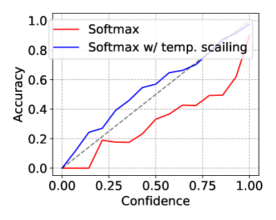
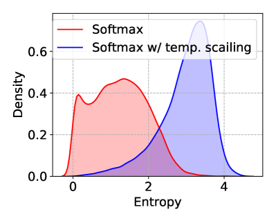
Figure 1: Reliability curve (left) and predictive uncertainty on out-of-distribution samples (right) of ResNet.

Unfortunately, it is widely known that neural networks produce uncalibrated predictive uncertainty. For example, Figure 1 illustrates the uncalibrated predictive behavior of ResNet (He et al., 2016): its confidence tends to higher than its accuracy (Figure 1 (left)); also, it provides low predictive entropy on OOD samples (Figure 1 (right)). Due to this problem, interpretation of $\phi^{{\bm{W}}}({\mathbf{x}})$ as the “predictive probability” is often considered as implausible (Gal & Ghahramani, 2016).

2.2 Temperature Scaling

One simple yet effective solution for improving the predictive probability’s quality is to use post-hoc calibration methods. Among them, temperature scaling (Guo et al., 2017) adjusts the smoothness of the softmax outputs for maximizing the log-likelihood on a holdout dataset $\mathcal{D}^{\prime}$:

$$\max_{\tau}\sum_{({\bm{x}},y)\in\mathcal{D}^{\prime}}\log\frac{\exp(f_{y}^{{\bm{W}}}({\bm{x}})/\tau)}{\sum_{j}\exp(f_{j}^{{\bm{W}}}({\bm{x}})/\tau)}$$ (4)

where ${\bm{W}}$ is a fixed pretrained weight and $\tau$ is a temperature controlling the smoothness of the softmax output.

Figure 1 illustrates the effectiveness of the temperature scaling on providing a better calibrated predictive uncertainty: the confidence closely matches its actual accuracy and the predictive entropy on OOD samples significantly increases. However, the post-hoc calibration methods have some inherent disadvantages: the performance is sensitive to the quality of the holdout dataset; also, they cannot utilize full training data, which could result in lower generalization performance. For these reasons, we explore an alternative approach that does not require the post-hoc calibration.

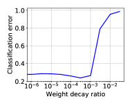
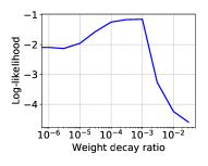
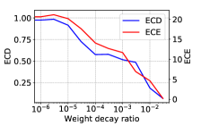
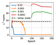
Figure 2: Impacts of the weight decay rate on accuracy (a), log-likelihood (b), calibration performance (c), and and the $L^{2}$ norm (d).

3 Motivation

Motivated by the temperature scaling, we closely analyze how the log-likelihood is related to the calibration performance. To this end, let ${\textnormal{s}}_{{\mathbf{x}}}$ be a binary random variable indicating whether a model correctly classifies a sample ${\mathbf{x}}$; $p(s_{\mathbf{x}})=p({\textnormal{y}}=\operatorname*{arg\,max}_{k}\phi^{{\bm{W}}}_{k}({\mathbf{x}}))$ where y is a true label of ${\mathbf{x}}$. Then, we can derive the following inequality by using the law of total expectation:

$$\begin{split}\mathbb{E}_{{\mathbf{x}},{\textnormal{y}}}[\log\phi^{{\bm{W}}}_{{\textnormal{y}}}({\mathbf{x}})]=\mathbb{E}_{{\mathbf{x}}}\left[\mathbb{E}_{{\textnormal{s}}}\left[\mathbb{E}_{{\textnormal{y}}}[\log\phi^{{\bm{W}}}_{{\textnormal{y}}}({\mathbf{x}})|{\textnormal{s}}_{{\mathbf{x}}},{\mathbf{x}}]|{\mathbf{x}}\right]\right]\\ \leq\mathbb{E}_{{\mathbf{x}}}[p(s_{{\mathbf{x}}})\log\phi^{{\bm{W}}}_{m_{{\mathbf{x}}}}({\mathbf{x}})+p(\neg s_{{\mathbf{x}}})\log(1-\phi^{{\bm{W}}}_{m_{{\mathbf{x}}}}({\mathbf{x}}))]\end{split}$$ (5)

where $m_{{\mathbf{x}}}=\operatorname*{arg\,max}_{k}\phi^{{\bm{W}}}_{k}({\mathbf{x}})$ and the inequality comes from the fact that $\mathbb{E}_{{\textnormal{y}}}\left[\log\phi^{{\bm{W}}}_{{\textnormal{y}}}({\mathbf{x}})|\neg s_{\mathbf{x}},{\mathbf{x}}\right]\leq\max_{k\neq m_{{\mathbf{x}}}}\log\phi^{{\bm{W}}}_{k}({\mathbf{x}})\leq\log\left(1-\phi^{{\bm{W}}}_{m_{{\mathbf{x}}}}({\mathbf{x}})\right)$.

Consider we apply the inequality in equation 5 to the log-likelihood on test samples $\mathcal{D}^{T}$. Suppose we group predictions based on the confidence such that ${\bm{x}},{\bm{x}}^{\prime}\in\mathcal{G}_{k}^{\epsilon}\rightarrow|\log\phi^{\bm{W}}_{m_{\bm{x}}}-\log\phi^{\bm{W}}_{m_{{\bm{x}}^{\prime}}}|<\epsilon$ for arbitrary small $\epsilon$ and some $k$. Then, we can approximate the upper bound by:

$$\hat{\mathbb{E}}_{\mathcal{D}^{T}}\left[p(s_{{\mathbf{x}}})\log\phi^{{\bm{W}}}_{m_{{\mathbf{x}}}}({\mathbf{x}})+p(\neg s_{{\mathbf{x}}})\log(1-\phi^{{\bm{W}}}_{m_{{\mathbf{x}}}}({\mathbf{x}}))\right]\\ \approx-\sum_{i=1}^{M^{\epsilon}}\frac{|\mathcal{G}^{\epsilon}_{i}|}{N^{T}}CE(\text{acc}(\mathcal{G}^{\epsilon}_{i})\parallel\text{conf}(\mathcal{G}^{\epsilon}_{i}))$$ (6)

where $\hat{\mathbb{E}}_{\mathcal{D^{T}}}[\cdot]$ is the empirical mean on $\mathcal{D}^{T}$, $|\mathcal{G}^{\epsilon}_{i}|$ is the number of samples in $\mathcal{G}^{\epsilon}_{i}$, $N^{T}$ is the number of test samples, $M^{\epsilon}$ is a number of groups given $\epsilon$, and $CE(\cdot\parallel\cdot)$ is a cross-entropy.

This upper bound can be thought of as the probabilistic measure of calibration performance, and we refer to its negative value as expected calibration divergence (ECD). Specifically, consider a neural network that produces an answer with probability $\text{conf}(\mathcal{G}^{\epsilon}_{i})$ and refuses to answer otherwise. Then, ECD becomes the expected divergence between the model’s ability to correctly predict the sample and the model’s willingness to answer.

The above analysis suggests that improving the log-likelihood on test samples can lead to a better-calibrated model. This means that we can focus on generalization of the training objective for improving the calibration performance. To achieve this, we explore explicit regularization techniques for improving the log-likelihood on unseen samples. We remark that our approach is fundamentally different from previous regularization research in deep learning concentrating on the effects of regularization on generalization performance, which treats the log-likelihood as a surrogate loss for improving accuracy.

4 Regularization by Strong Weight Decay

Weight decay (Krogh & Hertz, 1992) is one of the most widely used explicit regularization techniques, which is already involved in many benchmark models. However, we conjecture that the decay rate in benchmark training strategies, e.g., 0.0001 in ResNet, is too small to induce a regularization effect. Therefore, we investigate the impacts of a large weight decay rate on log-likelihood and calibration performance.

Figure 2 illustrates the impact of the weight decay rate $\lambda$ on generalization performance (a), log-likelihood (b), and calibration performance (c). Specifically, in the region of $\lambda\leq 0.001$, a stronger weight decay improves the log-likelihood. Also, as in the theoretical analysis in Section 3, the log-likelihood improvement results in better calibration performance in terms of both ECD and ECE. However, these improvements become inversely proportional to the accuracy improvement when $\lambda>0.001$ (which is only 10x larger than a base decay ratio).

To more thoroughly investigate this undesirability, we further analyze the impact of weight decay on the $L^{2}$ function norm of $f^{\bm{W}}$. Here, the $L^{2}$ norm of $f^{\bm{W}}$ is defined as $\parallel f^{{\bm{W}}}\parallel_{2}=\left(\int|f^{{\bm{W}}}({\bm{x}})|^{2}dP_{{\mathbf{x}}}({\bm{x}})\right)^{1/2}$, which we will discuss with more detail in Section 5. In this work, we compute $L^{2}$ norm by the Monte-Carlo approximation since we do not have access to a data-generating distribution $P_{{\mathbf{x}}}({\bm{x}})$.

To set a desired value of $L^{2}$ norm, we first note that temperature scaling modifies only $L^{2}$ norm without affecting the accuracy (cf. equation 4). We also note that moderate changes in $\lambda$ do not greatly impact the generalization error (cf. Figure 2 (a)). Therefore, the calibrated $L^{2}$ norm obtained by applying temperature scaling on the test set $\mathcal{D}^{T}$ can be thought of as the target complexity for maximizing the log-likelihood given certain generalization performance of $f^{{\bm{W}}}$, for which we want to achieve by varying $\lambda$.

In Figure 2 (d), we monitor $\parallel f^{{\bm{W}}}\parallel_{2}$ under all considered weight decay rates, which shows that the SGD with various decay rates finds only a trivial solution or an infeasible solution to the following optimization problem:

$$\max_{{\bm{W}}}\hat{\mathbb{E}}_{\mathcal{D}}\left[\log\phi_{{\textnormal{y}}}^{{\bm{W}}}({\mathbf{x}})\right]\quad$$

$$\text{s.t.}\parallel f^{{\bm{W}}}\parallel_{2}\leq\parallel f^{{{\bm{W}}^{\prime}}}/\tau^{*}\parallel_{2}$$ (7)

where ${\bm{W}}^{\prime}$ is the trained weights with $\lambda=0.0001$, and $\tau^{*}=\operatorname*{arg\,max}_{\tau}\hat{\mathbb{E}}_{\mathcal{D}^{T}}\left[\log\left\{\sigma(f^{{{\bm{W}}^{\prime}}}_{{\textnormal{y}}}({\mathbf{x}})/\tau)\right\}\right]$. Specifically, Figure 2 (d) shows that the $L^{2}$ norm goes to zero under the decay rate $\lambda\geq 0.003$, which means that all weights collapse to zero, i.e., the trivial solution. This happens when the magnitude of the decay rate overwhelms the magnitude of the weight update by the gradient of the log-likelihood, e.g., at approximately the epoch 50 under $\lambda=0.003$ (Figure 2 (d)). In the case of $\lambda\leq 0.001$, SGD with $\lambda$ does not suffer from the weight collapse, but the scale of the $L^{2}$ norm under such rates is significantly higher than $\parallel f^{{{\bm{W}}^{\prime}}}/\tau^{*}\parallel_{2}$, which corresponds to infeasible solutions (Figure 2 (d)).

We may overcome this undesirability by using a dynamic weight decay rate for each parameter that adjusts the decay rate corresponding to its overall gradient scale, which can prevent the weight collapse while reducing the $L^{2}$ norm. However, this approach requires a rule for the decay rate update (or a meta-learning algorithm with additional parameters). Thus, we will explore alternative forms of explicit regularization that directly penalize the function complexity.

5 Direct Regularization of Function Complexity

5.1 Regularization in the Function Space

The first approach regards $f^{{\bm{W}}}$ as an element of $L^{p}(\mathcal{X})$ space. $L^{p}$ space is the space of measurable functions with the norm:

$$\parallel f^{{\bm{W}}}\parallel_{p}=\left(\int_{\mathcal{X}}|f^{{\bm{W}}}({\bm{x}})|^{p}dP_{{\mathbf{x}}}({\bm{x}})\right)^{1/p}<\infty.$$ (8)

As aforementioned, we use Monte-Carlo approximation for computing $L^{p}$ norm, which can be computed as $\parallel f^{{\bm{W}}}\parallel_{p}^{p}\approx\frac{1}{m}\sum_{i,j}|f^{{\bm{W}}}_{j}({\bm{x}}^{(i)})|^{p}$. In this paper, we examine $\parallel f^{{\bm{W}}}\parallel_{1}$ and $\parallel f^{{\bm{W}}}\parallel_{2}^{2}$ regularization losses.

We note that the norm is computed with respect to the input generating distribution $P_{{\mathbf{x}}}$. Therefore, if the function complexity approximated with the training distribution does not reflect its true complexity on $P_{{\mathbf{x}}}$, regularizing the $L^{p}$ norm during training could be meaningless. Fortunately, we observe that function’s properties, which depends only on ${\mathbf{x}}$, evaluated on two different datasets drawn from the identical distribution are very close to each other compared to values that depend on the external randomness ${\textnormal{y}}|{\mathbf{x}}$. For example, the empirical mean of the maximum log-probability $\log\phi^{{\bm{W}}}_{m_{{\mathbf{x}}}}({\mathbf{x}})$ (Figure 3 (left)) and $L^{2}$ norm of $f^{{\bm{W}}}$ (Figure 3 (right)) on training samples are significantly similar to those values on unseen samples compared to the log-likelihood (Figure 3 (left)).

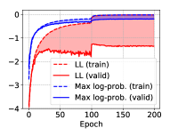
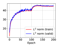
Figure 3: Monitoring changes in the behavior of ResNet during training on CIFAR-100. LL indicates the log-likelihood $\mathbb{E}_{{\mathbf{x}},{\textnormal{y}}}[\log\phi^{{\bm{W}}}_{{\textnormal{y}}}({\mathbf{x}})]$ and max log-prob indicates $\mathbb{E}_{{\mathbf{x}}}[\log\phi^{{\bm{W}}}_{m_{{\mathbf{x}}}}({\mathbf{x}})]$.

Table 1: Experimental results under various regularization methods on ResNet. Arrows on the metrics represent the desirable direction. $\lambda^{*}$ represents the best hyperparameter.

	CIFAR-10					CIFAR-100
method	Acc $\uparrow$	NLL $\downarrow$	ECE $\downarrow$	$\parallel f^{{\bm{W}}}\parallel_{2}$	$\lambda^{*}$	Acc $\uparrow$	NLL $\downarrow$	ECE $\downarrow$	$\parallel f^{{\bm{W}}}\parallel_{2}$	$\lambda^{*}$
ResNet-50	94.17	0.29	4.06	20.12	-	74.64	1.31	13.95	43.81	-
+ $\parallel f^{{\bm{W}}}\parallel_{1}$	94.32	0.25	2.89	6.81	0.01	76.28	1.27	7.77	9.07	0.01
+ $\parallel f^{{\bm{W}}}\parallel_{2}^{2}$	94.38	0.23	3.27	8.19	0.003	75.84	1.07	5.52	10.55	0.01
+ $SW_{1}(\mu^{{\bm{W}}}_{\mathcal{D}^{\prime}},\nu)$	94.46	0.23	2.12	5.4	0.001	76.27	1.1	7.02	9.67	0.01
+ PER	94.30	0.23	2.89	6.94	0.03	76.23	1.15	4.67	7.56	1.0
VGG-16	92.97	0.35	4.96	9.62	-	71.96	1.4	16.9	22.98	-
+ $\parallel f^{{\bm{W}}}\parallel_{1}$	93.07	0.33	4.1	6.62	0.01	72.71	1.44	11.37	9.27	0.03
+ $\parallel f^{{\bm{W}}}\parallel_{2}^{2}$	93.06	0.31	4.58	7.44	0.003	72.68	1.31	10.79	9.28	0.01
+ $SW_{1}(\mu^{{\bm{W}}}_{\mathcal{D}^{\prime}},\nu)$	93.13	0.29	1.9	5.4	0.001	72.26	1.35	12.59	9.72	0.03
+ PER	93.1	0.31	4.79	8.49	0.003	72.89	1.34	6.47	7.37	1.0

5.2 Regularization in the Probability Distribution Space

The second approach regards $f^{{\bm{W}}}({\mathbf{x}})$ as a random variable and then minimizes its distance to the bell-shaped target distribution (e.g., the standard Gaussian). Since the bell-shaped distribution has a peak mass at zero, this regularization encourages logits to have small values, making $\parallel f^{{\bm{W}}}\parallel_{2}$ small. It also has additional regularization effects such as decorrelating logits and producing high predictive entropy.

As a metric in the probability distribution space, we use the sliced Wasserstein distance of order one because of its computational efficiency and ability to measure the distance between probability distributions with different supports, which is useful when dealing with the empirical distribution. We refer to Peyré et al. (2019) for more detailed explanations about this metric.

Given minibatch samples $\mathcal{D}^{\prime}=\{{\bm{x}}^{(i)}\}^{m}_{i=1}$, we denote an empirical measure of logits as $\mu_{\mathcal{D}^{\prime}}({\mathbb{A}}):=\frac{1}{m}\sum_{i}\mathbbm{1}_{{\mathbb{A}}}(f^{{\bm{W}}}({\bm{x}}^{(i)}))$ and the standard Gaussian measure on $\mathcal{Z}$ as $\nu^{\mathcal{Z}}({\mathbb{A}}):=\frac{1}{2\pi^{K/2}}\int_{{\mathbb{A}}}\exp\left(-\frac{1}{2}\parallel{\bm{z}}\parallel^{2}\right)d{\bm{z}}$. Then, the sliced Wasserstein distance between them is given by:

$$SW_{1}(\mu_{\mathcal{D}^{\prime}},\nu^{\mathcal{Z}})=\int_{\mathbb{S}^{K-1}}\int_{\mathbb{R}}\left|F_{\mu_{\mathcal{D}^{\prime}}^{\theta}}(x)-F_{\nu^{\mathbb{R}}}(x)\right|dxd\lambda(\theta)$$ (9)

where ${\bm{z}}^{(i)}=f^{{\bm{W}}}({\bm{x}}^{(i)})$, $\mu_{\mathcal{D}^{\prime}}^{\theta}$ is a measure obtained by projecting $\mu_{\mathcal{D}^{\prime}}$ at angle $\theta$, $F_{\mu}$ is a cumulative distribution function of a probability measure $\mu$, and $\lambda$ is a uniform measure on the unit sphere $\mathbb{S}^{K-1}$. In this work, the integration over $\mathbb{S}^{K-1}$ is evaluated by Monte-Carlo approximation with 256 number of evaluations, following Joo et al. (2020b).

We also consider projected error function regularization (PER) (Joo et al., 2020b) that simplifies the computation of $SW_{1}(\mu_{\mathcal{D}^{\prime}},\nu^{\mathcal{Z}})$ by applying the Minkowski inequality to equation 9. PER can be thought of as computing a robust norm in a randomly projected space induced by $\theta\sim P_{\lambda}$, which combines advantages of both the $L^{1}$ norm and the $L^{2}$ norm as well as captures the dependency between logits of each location by a random projection operation.

6 Experiments

In this section, we examine the effectiveness of the function complexity regularization on improving the calibration performance. Throughout this section, we report mean values (rounded to two decimal places) obtained from five repetitions, and the experiments were performed on a single workstation with 8 GPUs (NVIDIA GeForce RTX 2080 Ti). We also note that all regularization methods do not result in a notable running time difference compared to the vanilla method, so we omit the running time comparison. To support reproducibility, we submit the code and will make it publicly available after the review period.

6.1 Image Classification with ResNet and VGG

We first consider the image-classification task on CIFAR (Krizhevsky et al., 2009). We used the (pre-activation) ResNet (He et al., 2016), which is one of the most prevalent basis architectures in many state-of-the-art architectures (Huang et al., 2017; Xie et al., 2017). We also examined the VGG (Simonyan & Zisserman, 2015) as a representative of models without a residual connection.

Setup. We follow the training strategy presented in He et al. (2016): we trained the model for 200 epochs by SGD with momentum coefficient 0.9, minibatch size of 128, and a weight decay rate 0.0001; weights were initialized as in He et al. (2015); an initial learning rate was 0.1, and decreased by a factor of 10 at 100 and 150 epochs. We also used the augmentation presented in He et al. (2015). In addition to the standard configuration, we used the initial learning rate warm-up, clipped the gradient when its norm exceeds one and made an extra validation set of 10,000 samples split from the training set. For convenience, we re-used this configuration for VGG-training except increasing the weight decay rate to 0.0005 as in Simonyan & Zisserman (2015).

We chose a regularization coefficient based on the validation set accuracy among the following four coefficients for each method: $\{0.1,0.03,0.01,0.003\}$ for $L^{1}$ norm and sliced Wasserstein regularizations; $\{0.03,0.01,0.003,0.001\}$ for $L^{2}$ norm regularization; $\{1.0,0.3,0.1,0.03\}$ for PER (10x lower for CIFAR-10).

We evaluate methods by classification error, negative log-likelihood (NLL), and ECE, which are commonly used in literature (Lakshminarayanan et al., 2017; Guo et al., 2017; Ovadia et al., 2019). We note that we do not use ECD as a performance measure since its role was to derive motivation for improving generalization of the training objective with explicit regularization and it has a strong correlation with ECE (cf. Figure 2 (c)).

Table 2: Experimental results under various regularization methods on BERT. Arrows on the metrics represent the desirable direction. $\lambda^{*}$ represents the best hyperparameter.

	20-Newsgroup					Web of science
method	Acc $\uparrow$	NLL $\downarrow$	ECE $\downarrow$	$\parallel f^{{\bm{W}}}\parallel_{2}$	$\lambda^{*}$	Acc $\uparrow$	NLL $\downarrow$	ECE $\downarrow$	$\parallel f^{{\bm{W}}}\parallel_{2}$	$\lambda^{*}$
BERT	84.51	0.70	6.40	9.71	-	81.28	0.94	8.26	20.13	-
+ $\parallel f^{{\bm{W}}}\parallel_{1}$	84.71	0.61	4.67	6.02	0.1	81.68	0.90	7.02	8.89	0.1
+ $\parallel f^{{\bm{W}}}\parallel_{2}^{2}$	85.04	0.64	3.24	5.11	0.1	81.83	0.94	5.79	7.70	0.1
+ $SW_{1}(\mu^{{\bm{W}}}_{\mathcal{D}^{\prime}},\nu)$	84.76	0.67	3.78	4.98	0.1	81.44	0.89	7.22	11.33	0.1
+ PER	85.02	0.65	4.50	6.21	0.3	81.36	0.87	8.19	13.21	0.3

Results. Table 1 lists the experimental results, in which both regularization in the function space and the Wasserstein probability space successfully reduced the function complexity, e.g., reduced the $L^{2}$ norm of ResNet by at least 34% on CIFAR-10 and 68% on CIFAR-100. We note that regularization methods reduce the function complexity without compromising the generalization performance, unlike weight decay; that is, all regularization methods achieves consistent improvements of test error rates. We also note that the sum of the Frobenius norm of weights often increases compared to the vanilla method and changes only at most 2% when it decreases, which again shows the undesirability of adjusting the weight decay rate for the function complexity regularization.

More importantly, the predictive probability’s quality under explicit regularization is significantly better than the quality under the vanilla method. For instance, the regularization methods reduce the NLL of ResNet by at least 13% CIFAR-10 and 6% on CIFAR-100 and reduce the ECE of ResNet by at least 19% on CIFAR-10 and 41% on CIFAR-100. These improvements are comparable to or better than those of temperature scaling. For instance, temperature scaling gives NLL of 1.15 and ECE of 8.41 on CIFAR-100.

We can also see that all regularization losses improve NLL, ECE, and accuracy of VGG, except $L^{1}$ regularization on CIFAR-100 (Table 1). However, the effectiveness of explicit regularization on VGG tends to be less significant compared to their effects on ResNet. This might be contributed to a small capacity of VGG, which can be inferred from that $\parallel f^{{\bm{W}}}\parallel_{2}$ of VGG that is reduced by almost 50% compared to ResNet.

6.2 Document Classification with BERT

We also perform experiments on the natural language processing domain in order to more thoroughly evaluate the effectiveness of explicit regularization. Inspired by the recent finding (Kong et al., 2020), we perform document classification on 20 newsgroup dataset (Socher et al., 2012) and web of science dataset (Kowsari et al., 2017). We obtain a classifier by adding a linear layer and a softmax to BERT (Devlin et al., 2018).

Setup. Our configuration is based on Kong et al. (2020): we initialize the model by the pretrained BERT, and then the model is trained for 5 epochs by Adam optimizer (Kingma & Ba, 2015) with learning rate 0.00005 ($\beta_{1}=0.9,\beta_{2}=0.999$) and minibatch size of 32.

The search spaces of regularization coefficients were: $\{0.3,0.1,0.003,0.001\}$ for $L^{1}$ norm, $L^{2}$ norm sliced Wasserstein regularizations; $\{1.0,0.3,0.1,0.003\}$ for PER.

Result. As consistent with the findings in the image classification task, all explicit regularization methods improve the reliability of predictive probability with consistent gains in test accuracy (Table 2). We believe the consistent results on two different domains (image classification and document classification) corroborate the significance of our findings, leaving extensive evaluation on more diverse environments as future work.

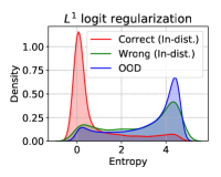
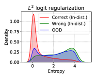
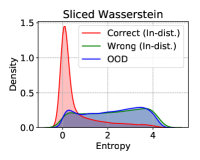
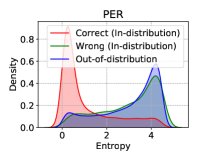
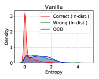
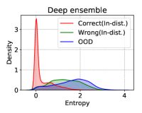
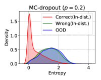
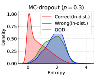
Figure 4: Density of predictive uncertainty on CIFAR-100 (in-distribution) and SVHN (OOD). The upper figures illustrate explicit regularization methods, and the lower figures illustrate the vanilla method, ensemble methods, and Bayesian neural networks.

Table 3: Misclassification detection and OOD detection task performances based on NBAUCC_0.5. Arrows on the metrics represent the desirable direction. We present the result of MC-dropout with probability $0.3$, which performed best among $p\in\{0.2,0.3,0.5\}$.

Task	Vanilla	MC-dropout	Deep Ensemble	$\parallel f^{{\bm{W}}}\parallel_{1}$	$\parallel f^{{\bm{W}}}\parallel_{2}^{2}$	$SW_{1}(\mu^{{\bm{W}}}_{\mathcal{D}^{\prime}},\nu)$	PER
Misclasification detection $\uparrow$	1.55	5.94	0.59	9.53	6.85	5.10	10.24
OOD detection $\uparrow$	15.98	31.28	28.46	55.51	31.47	31.63	49.77

6.3 Predictive Uncertainty on Ignorant Samples

We analyze the predictive uncertainty of ResNet-50 on misclassified samples and OOD samples, expecting it to produce the answer of “I don’t know” for these samples (Figure 4). We can see that the vanilla method provides somewhat low predictive entropy for OOD and misclassified samples, albeit the entropy is slightly higher than the entropy on correctly classified samples. In contrast, explicit regularization successfully gathers a mass of predictive entropy for both OOD samples and misclassified samples around the maximum-entropy region.

We compare predictive uncertainty under explicit regularization to those of Bayesian neural networks and ensemble methods. Specifically, we use the scalable Bayesian neural network, called MC-dropout (Gal & Ghahramani, 2016), because other methods based on variational inference (Graves, 2011; Blundell et al., 2015; Wu et al., 2019) or MCMC (Welling & Teh, 2011; Zhang et al., 2020) require modifications to the baseline including the optimization procedure and the architecture, which deters a fair comparison. We searched a dropout rate over {0.1, 0.2, 0.3, 0.4, 0.5 } and used 100 number of Monte-Carlo samples at test time, i.e., 100x more inference time. We also use the deep ensemble (Lakshminarayanan et al., 2017) with 5 number of ensembles, i.e., 5x more training and inference time.

Figure 4 shows that the regularization-based methods produce significantly better uncertainty representation than the MC-dropout and deep ensemble; even though both deep ensemble and MC-dropout can move mass on less certain regions, the positions are still far from the highest uncertainty region, unlike the regularization-based methods.

For quantitative evaluation of the uncertainty representation ability, we measure misclassification and OOD detection performances. To this end, we use recently proposed normalized bounded area under the calibration curve (NBAUCC) (Kong et al., 2020), which overcomes a disadvantage of classical measures such as AUROC and AUPRC that cannot consider the calibration performance. Specifically, NBAUCC with the upper bound of confidence threshold for misclassified or OOD samples, denoted by $\tau$, is computed by:

$$\text{NBAUCC}_{\tau}=\frac{1}{M}\sum_{i=1}^{M}F_{1}\left(\frac{\tau}{M}i\right)$$ (10)

where $F_{1}(t)$ computes $F_{1}$ score by regarding samples with predictive confidence higher than $\tau$ as correct (resp. in-distribution) samples and incorrect (resp. OOD) samples otherwise; $M$ is a predetermined step size. We present the misclassification and OOD detection performances in Table 3, where all regularization methods significantly improve detection performances based on their better predictive uncertainty representation abilities.

6.4 Comparison to Implicit Regularization

Various forms of implicit regularization in deep learning have shown promising theoretical and empirical results on improving generalization performance (Hardt et al., 2016; Hoffer et al., 2017; Gunasekar et al., 2018; Li et al., 2019). In this regard, we investigate their potential impacts on the calibration performance by magnifying implicit regularization effects of early stopping and SGD in ResNet-50.

Figure 5 shows that the early stopping does not result in dramatic improvements, unlike PER. On CIFAR-10, NLL and ECE are improved compared to the baseline, but these improvements are marginal compared to PER. On the contrary, on CIFAR-100, a longer training slightly benefits NLL and ECE due to increased classification accuracy. Considering that the $L^{2}$ norm achieves a significantly high value at the early stage of training (cf. Figure 3 (right)), this undesirable result may seem natural.

Next, we examine the effects of varying minibatch sizes under the baseline learning rate or linear scaling rule (Goyal et al., 2017), in which a smaller minibatch size increases the noise of the stochastic gradient. In Figure 6, we observe that increasing the noise level by using smaller batch sizes benefits generalization performance. However, it does not benefit and even worsens the predictive distribution quality (NLL and ECE). These observations highlight the importance of explicit regularization for improving the calibration performance of neural networks.

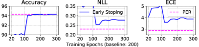
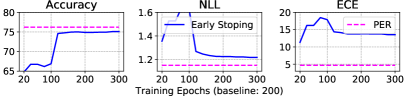
Figure 5: Impacts of early stopping on accuracy, negative log-likelihood, and ECE in CIFAR-10 (upper) and CIFAR-100 (lower). X-axis represents the maximum number of training epochs.

7 Related Work

Recent works show that joint modeling of a generative model $p({\mathbf{x}})$ along with a classifier $p({\textnormal{y}}|{\mathbf{x}})$, or $p({\mathbf{x}},{\textnormal{y}})$ directly, helps to produce calibrated predictive uncertainty (Alemi et al., 2018; Nalisnick et al., 2019; Grathwohl et al., 2020). Specifically, Alemi et al. (2018) argue that modeling stochastic hidden representation through the variational information bottleneck principle (Alemi et al., 2017) allows representing better predictive uncertainty. This can be related to the effectiveness of ensemble methods for well-calibrated predictive uncertainty, which aggregate representations of several models (Lakshminarayanan et al., 2017; Ovadia et al., 2019; Ashukha et al., 2020). In this regard, hybrid modeling and ensemble methods share a similar principle to the Bayesian methods, concerning the stochasticity of the function. However, this paper takes a fundamentally different approach that concentrates on explicit regularization in deterministic neural networks.

Other works concentrate on the structural characteristics of neural networks. Specifically, Hein et al. (2019) identify the cause of the overconfidence problem based on an analysis of the affine compositional function, e.g., ReLU. The basic intuition behind this analysis is that one can always find a multiplier $\lambda$ to an input ${\bm{x}}$, which makes a neural network produce one dominant entry on $\lambda{\bm{x}}$. Verma & Swami (2019) point out that the region of the highest predictive uncertainty under the softmax forms a subspace in the logit space, so the volume of an area representing high predictive uncertainty would be negligible. However, our approach suggests that these structural characteristics’ inherent flaws can be easily cured by adding an explicit regularization term without changing the existing components of neural networks.

From the perspective of the statistical learning theory (Vapnik, 1995), a regularization method minimizing some form of complexity measures, e.g., Rademacher complexity (Bartlett et al., 2005) or VC-dimension (Vapnik & Chervonenkis, 2015), is required to achieve better generalization of overparameterized models by preventing memorization of intricate patterns existing only in training samples. However, the role of capacity control with explicit regularization is challenged by many observations in deep learning. Specifically, overparameterized neural networks achieve impressive generalization performance with only implicit regularizations contained in the optimization procedures (Hardt et al., 2016; Li et al., 2019) or the structural characteristics (Gunasekar et al., 2018; Hanin & Rolnick, 2019; Luo et al., 2019). Moreover, Zhang et al. (2017) show that explicit regularization does not prevent neural networks from fitting random labels that cannot be generalized to unseen examples. Therefore, the importance of explicit regularization in deep learning seems to be questionable. In this work, we reemphasize its importance, presenting a different view on the role of regularization that improves predictive uncertainty representation.

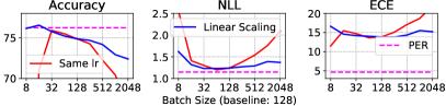
Figure 6: Impacts of varying noise in stochastic gradient computation on accuracy, negative log-likelihood, and ECE in CIFAR-100.

8 Conclusion

In this works, we show the effectiveness of explicit regularization on improving the calibration of predictive uncertainty, which presents a novel view on the role and importance of explicit regularization. Specifically, our extensive experimental results show that explicit regularization methods improve calibration performance, predictive uncertainty representation, misclassification/OOD detection performances, and even test accuracy. The regularization-based approach has better computational efficiency and scalability compared to Bayesian neural networks and ensemble methods. Also, it is not subject to the quality of the holdout dataset, unlike post-hoc calibration methods. However, the regularization methods are limited in that they cannot utilize more sophisticated uncertainty quantification methods due to its deterministic nature, such as mutual information measuring epistemic uncertainty (Smith & Gal, 2018). We leave this limitation as an important future direction of research, which may be solved by using more expressive parameterization in the last layer, e.g., (Wilson et al., 2016; Skafte et al., 2019; Malinin & Gales, 2019; Joo et al., 2020a).

References

- Alemi et al. (2017) Alemi, A. A., Fischer, I., Dillon, J. V., and Murphy, K. Deep variational information bottleneck. In International Conference on Learning Representations, 2017.
- Alemi et al. (2018) Alemi, A. A., Fischer, I., and Dillon, J. V. Uncertainty in the variational information bottleneck. arXiv preprint arXiv:1807.00906, 2018.
- Ashukha et al. (2020) Ashukha, A., Lyzhov, A., Molchanov, D., and Vetrov, D. Pitfalls of in-domain uncertainty estimation and ensembling in deep learning. In International Conference on Learning Representations, 2020.
- Bartlett et al. (2005) Bartlett, P. L., Bousquet, O., Mendelson, S., et al. Local Rademacher complexities. The Annals of Statistics, 33(4):1497–1537, 2005.
- Blundell et al. (2015) Blundell, C., Cornebise, J., Kavukcuoglu, K., and Wierstra, D. Weight uncertainty in neural networks. In International Conference on Machine Learning, 2015.
- Bridle (1990) Bridle, J. S. Probabilistic interpretation of feedforward classification network outputs, with relationships to statistical pattern recognition. In Neurocomputing, pp. 227–236. Springer, 1990.
- Dawid (1982) Dawid, A. P. The well-calibrated Bayesian. Journal of the American Statistical Association, 77(379):605–610, 1982.
- Devlin et al. (2018) Devlin, J., Chang, M.-W., Lee, K., and Toutanova, K. Bert: Pre-training of deep bidirectional transformers for language understanding. arXiv preprint arXiv:1810.04805, 2018.
- Gal & Ghahramani (2016) Gal, Y. and Ghahramani, Z. Dropout as a Bayesian approximation: Representing model uncertainty in deep learning. In International Conference on Machine Learning, 2016.
- Goodfellow et al. (2015) Goodfellow, I. J., Shlens, J., and Szegedy, C. Explaining and harnessing adversarial examples. In International Conference on Learning Representations, 2015.
- Goyal et al. (2017) Goyal, P., Dollár, P., Girshick, R., Noordhuis, P., Wesolowski, L., Kyrola, A., Tulloch, A., Jia, Y., and He, K. Accurate, large minibatch sgd: Training imagenet in 1 hour. arXiv preprint arXiv:1706.02677, 2017.
- Grathwohl et al. (2020) Grathwohl, W., Wang, K.-C., Jacobsen, J.-H., Duvenaud, D., Norouzi, M., and Swersky, K. Your classifier is secretly an energy based model and you should treat it like one. In International Conference on Learning Representations, 2020.
- Graves (2011) Graves, A. Practical variational inference for neural networks. In Advances in Neural Information Processing Systems, 2011.
- Gunasekar et al. (2018) Gunasekar, S., Lee, J. D., Soudry, D., and Srebro, N. Implicit bias of gradient descent on linear convolutional networks. In Advances in Neural Information Processing Systems, 2018.
- Guo et al. (2017) Guo, C., Pleiss, G., Sun, Y., and Weinberger, K. Q. On calibration of modern neural networks. In International Conference on Machine Learning, 2017.
- Hanin & Rolnick (2019) Hanin, B. and Rolnick, D. Deep relu networks have surprisingly few activation patterns. In Advances in Neural Information Processing Systems, 2019.
- Hardt et al. (2016) Hardt, M., Recht, B., and Singer, Y. Train faster, generalize better: Stability of stochastic gradient descent. In International Conference on Machine Learning, 2016.
- He et al. (2015) He, K., Zhang, X., Ren, S., and Sun, J. Delving deep into rectifiers: Surpassing human-level performance on imagenet classification. In IEEE International Conference on Computer Vision, 2015.
- He et al. (2016) He, K., Zhang, X., Ren, S., and Sun, J. Identity mappings in deep residual networks. In European Conference on Computer Vision, pp. 630–645, 2016.
- Hein et al. (2019) Hein, M., Andriushchenko, M., and Bitterwolf, J. Why relu networks yield high-confidence predictions far away from the training data and how to mitigate the problem. In IEEE Conference on Computer Vision and Pattern Recognition, 2019.
- Hoffer et al. (2017) Hoffer, E., Hubara, I., and Soudry, D. Train longer, generalize better: closing the generalization gap in large batch training of neural networks. In Advances in Neural Information Processing Systems, 2017.
- Huang et al. (2017) Huang, G., Liu, Z., Van Der Maaten, L., and Weinberger, K. Q. Densely connected convolutional networks. In IEEE Conference on Computer Vision and Pattern Recognition, 2017.
- Joo et al. (2020a) Joo, T., Chung, U., and Seo, M.-G. Being Bayesian about categorical probability. In International Conference on Machine Learning, 2020a.
- Joo et al. (2020b) Joo, T., Kang, D., and Kim, B. Regularizing activations in neural networks via distribution matching with the Wasserstein metric. In International Conference on Learning Representations, 2020b.
- Kingma & Ba (2015) Kingma, D. P. and Ba, J. Adam: A method for stochastic optimization. In International Conference on Learning Representations, 2015.
- Kong et al. (2020) Kong, L., Jiang, H., Zhuang, Y., Lyu, J., Zhao, T., and Zhang, C. Calibrated language model fine-tuning for in-and out-of-distribution data. In Conference on Empirical Methods in Natural Language Processing, 2020.
- Kowsari et al. (2017) Kowsari, K., Brown, D. E., Heidarysafa, M., Meimandi, K. J., Gerber, M. S., and Barnes, L. E. Hdltex: Hierarchical deep learning for text classification. In IEEE International Conference on Machine Learning and Applications, pp. 364–371. IEEE, 2017.
- Krizhevsky et al. (2009) Krizhevsky, A., Hinton, G., et al. Learning multiple layers of features from tiny images. 2009.
- Krogh & Hertz (1992) Krogh, A. and Hertz, J. A. A simple weight decay can improve generalization. In Advances in Neural Information Processing Systems, 1992.
- Lakshminarayanan et al. (2017) Lakshminarayanan, B., Pritzel, A., and Blundell, C. Simple and scalable predictive uncertainty estimation using deep ensembles. In Advances in Neural Information Processing Systems, 2017.
- Li et al. (2019) Li, Y., Wei, C., and Ma, T. Towards explaining the regularization effect of initial large learning rate in training neural networks. In Advances in Neural Information Processing Systems, 2019.
- Loshchilov & Hutter (2019) Loshchilov, I. and Hutter, F. Decoupled weight decay regularization. In International Conference on Learning Representations, 2019.
- Luo et al. (2019) Luo, P., Wang, X., Shao, W., and Peng, Z. Towards understanding regularization in batch normalization. In International Conference on Learning Representations, 2019.
- MacKay (1992) MacKay, D. J. A practical Bayesian framework for backpropagation networks. Neural Computation, 4(3):448–472, 1992.
- Malinin & Gales (2019) Malinin, A. and Gales, M. Reverse KL-divergence training of prior networks: Improved uncertainty and adversarial robustness. In Advances in Neural Information Processing Systems, 2019.
- Müller et al. (2019) Müller, R., Kornblith, S., and Hinton, G. When does label smoothing help? In Advances in Neural Information Processing Systems, 2019.
- Naeini et al. (2015) Naeini, M. P., Cooper, G., and Hauskrecht, M. Obtaining well calibrated probabilities using Bayesian binning. In AAAI Conference on Artificial Intelligence, 2015.
- Nalisnick et al. (2019) Nalisnick, E., Matsukawa, A., Teh, Y. W., Gorur, D., and Lakshminarayanan, B. Hybrid models with deep and invertible features. In International Conference on Machine Learning, 2019.
- Neal (1993) Neal, R. M. Bayesian learning via stochastic dynamics. In Advances in Neural Information Processing Systems, 1993.
- Osawa et al. (2019) Osawa, K., Swaroop, S., Khan, M. E. E., Jain, A., Eschenhagen, R., Turner, R. E., and Yokota, R. Practical deep learning with Bayesian principles. In Advances in Neural Information Processing Systems, 2019.
- Ovadia et al. (2019) Ovadia, Y., Fertig, E., Ren, J., Nado, Z., Sculley, D., Nowozin, S., Dillon, J., Lakshminarayanan, B., and Snoek, J. Can you trust your model’s uncertainty? evaluating predictive uncertainty under dataset shift. In Advances in Neural Information Processing Systems, 2019.
- Peyré et al. (2019) Peyré, G., Cuturi, M., et al. Computational optimal transport. Foundations and Trends® in Machine Learning, 11(5-6):355–607, 2019.
- Robbins & Monro (1951) Robbins, H. and Monro, S. A stochastic approximation method. The Annals of Mathematical Statistics, pp. 400–407, 1951.
- Simonyan & Zisserman (2015) Simonyan, K. and Zisserman, A. Very deep convolutional networks for large-scale image recognition. In International Conference on Learning Representations, 2015.
- Skafte et al. (2019) Skafte, N., Jørgensen, M., and Hauberg, S. Reliable training and estimation of variance networks. In Advances in Neural Information Processing Systems, 2019.
- Smith & Gal (2018) Smith, L. and Gal, Y. Understanding measures of uncertainty for adversarial example detection. arXiv preprint arXiv:1803.08533, 2018.
- Socher et al. (2012) Socher, R., Bengio, Y., and Manning, C. D. Deep learning for nlp (without magic). In Tutorial Abstracts of ACL 2012, pp. 5–5. 2012.
- Szegedy et al. (2016) Szegedy, C., Vanhoucke, V., Ioffe, S., Shlens, J., and Wojna, Z. Rethinking the inception architecture for computer vision. In IEEE Conference on Computer Vision and Pattern Recognition, 2016.
- Thulasidasan et al. (2019) Thulasidasan, S., Chennupati, G., Bilmes, J. A., Bhattacharya, T., and Michalak, S. On mixup training: Improved calibration and predictive uncertainty for deep neural networks. In Advances in Neural Information Processing Systems, 2019.
- Vapnik (1995) Vapnik, V. The Nature of Statistical Learning Theory. Springer-Verlag, 1995.
- Vapnik & Chervonenkis (2015) Vapnik, V. N. and Chervonenkis, A. Y. On the uniform convergence of relative frequencies of events to their probabilities. In Measures of Complexity, pp. 11–30. Springer, 2015.
- Verma & Swami (2019) Verma, G. and Swami, A. Error correcting output codes improve probability estimation and adversarial robustness of deep neural networks. In Advances in Neural Information Processing Systems, 2019.
- Welling & Teh (2011) Welling, M. and Teh, Y. W. Bayesian learning via stochastic gradient Langevin dynamics. In International Conference on Machine Learning, 2011.
- Wilson et al. (2016) Wilson, A. G., Hu, Z., Salakhutdinov, R. R., and Xing, E. P. Deep kernel learning. In International Conference on Artificial Intelligence and Statistics, 2016.
- Wu et al. (2019) Wu, A., Nowozin, S., Meeds, E., Turner, R. E., Hernández-Lobato, J. M., and Gaunt, A. L. Deterministic variational inference for robust Bayesian neural networks. In International Conference on Learning Representations, 2019.
- Xie et al. (2017) Xie, S., Girshick, R., Dollár, P., Tu, Z., and He, K. Aggregated residual transformations for deep neural networks. In IEEE Conference on Computer Vision and Pattern Recognition, 2017.
- Zhang et al. (2017) Zhang, C., Bengio, S., Hardt, M., Recht, B., and Vinyals, O. Understanding deep learning requires rethinking generalization. In International Conference on Learning Representations, 2017.
- Zhang et al. (2018) Zhang, H., Cisse, M., Dauphin, Y. N., and Lopez-Paz, D. Mixup: Beyond empirical risk minimization. In International Conference on Learning Representations, 2018.
- Zhang et al. (2020) Zhang, R., Li, C., Zhang, J., Chen, C., and Wilson, A. G. Cyclical stochastic gradient MCMC for Bayesian deep learning. In International Conference on Learning Representations, 2020.