The Free Uniform Spanning Forest is disconnected
in some virtually free groups, depending on the generator set

Abstract

We prove the rather counterintuitive result that there exist finite transitive graphs $H$ and integers $k$ such that the Free Uniform Spanning Forest in the direct product of the $k$-regular tree and $H$ has infinitely many trees almost surely.

This shows that the number of trees in the $\mathsf{FUSF}$ is not a quasi-isometry invariant. Moreover, we give two different Cayley graphs of the same virtually free group such that the $\mathsf{FUSF}$ has infinitely many trees in one, but is connected in the other, answering a question of Lyons and Peres [LP16] in the negative.

A version of our argument gives an example of a non-unimodular transitive graph where $\mathsf{WUSF}\not=\mathsf{FUSF}$, but some of the $\mathsf{FUSF}$ trees are light with respect to Haar measure. This disproves a conjecture of Tang [Tan19].

1 Intro

The Free Uniform Spanning Forest $\mathsf{FUSF}$ is one of the most standard random spanning forests of infinite graphs, obtained as the weak limit of the uniform random spanning trees $\mathsf{UST}$ in any exhaustion of the infinite graph by finite subgraphs. In any transitive graph, its law is invariant under the automorphisms of the graph. It may be regarded as the Free $\mathsf{FK}(p,q)$ random cluster model with $q=0$ at its critical point $p=0$, it is a determinantal process, and is especially interesting due to its connections to measurable group theory: in any Cayley graph of a group $\Gamma$, its expected degree is $2+2\beta^{(2)}_{1}(\Gamma)$, where $\beta^{(2)}_{1}(\Gamma)$ is the first $\ell^{2}$-Betti number of the group, the von Neumann dimension of the space of harmonic functions of finite Dirichlet energy. In particular, we have the equality $\mathsf{FUSF}=\mathsf{WUSF}$ with the Wired Uniform Spanning Forest iff $\beta^{(2)}_{1}(\Gamma)=0$. See [BLPS01] and [LP16, Chapter 10] for thorough studies of the $\mathsf{FUSF}$; some more recent papers are [HN17, Tim18, AHNR18, HN19].

We will mostly work in the direct product graph $\mathbb{T}^{k}\times H$, where $\mathbb{T}^{k}$ is the $k$-regular infinite tree with $k\geq 3$, while $H$ is a finite vertex-transitive graph. Typical examples are the product Cayley graphs of the virtually free groups $\mathbb{F}_{r}\times\Gamma$, where $\mathbb{F}_{r}$ is a free group on $r\geq 2$ generators and $\Gamma$ is a finite group. The $\mathsf{FUSF}$ on some tree-like graphs was recently studied, among other topics, in [Tan19]. In particular, Tang proved that, for any $k$, the $\mathsf{FUSF}$ in $\mathbb{T}^{k}\times\mathbb{Z}_{2}$ (where $\mathbb{Z}_{2}$ is the path on 2 vertices, i.e., a single edge) is connected almost surely; this was later generalized in [ABIT20+] for an arbitrary fixed weight on the $H$-edges. Tang made the innocent-looking conjecture that the connectedness holds more generally, for the direct product $\mathbb{T}^{k}\times H$ with any $k\geq 3$ and any finite transitive graph $H$ (no edge weights). See Remark 5.9 in that paper. Here we are disproving this conjecture.

Theorem 1.1 (Disconnected $\mathsf{FUSF}$).

For every $d$ there is $k_{d}$ such that if $\mathbb{T}^{k}$ is the $k$-regular infinite tree with $k\geq k_{d}$, and $H$ is a connected finite $d$-regular transitive graph on more than $k^{5/2}$ vertices, then the $\mathsf{FUSF}$ of $\mathbb{T}^{k}\times H$ is disconnected almost surely. In fact, it has infinitely many components.

One striking corollary of our result is that the number of trees in the $\mathsf{FUSF}$ of Cayley graphs is not a quasi-isometry invariant, as opposed to several similar properties: the number of trees in the $\mathsf{WUSF}$ [LP16, Corollary 10.25], the property $\mathsf{WUSF}\not=\mathsf{FUSF}$ [Soa93, BLPS01], or equivalently, the infinite-endedness of all the $\mathsf{FUSF}$ trees (the equivalence follows from [Mor03] and [HN17, Tim18]). (Note, nevertheless, that without transitivity of the graph the number of components is not a quasi-isometry invariant even when $\mathsf{WUSF}=\mathsf{FUSF}$, as the example in [Ben91] shows.) With some extra work, we prove here that the number of trees is not even the same for different Cayley graphs of a fixed group (even though the expected degree of the $\mathsf{FUSF}$ depends only on the group, because of the connection to $\beta^{(2)}_{1}(\Gamma)$). This answers a question of Lyons and Peres [LP16, Question 10.50] in the negative:

Theorem 1.2 (Dependence on the generating set).

For $k$ large enough, the group $\mathbb{F}_{k}\times\mathbb{Z}_{k^{9}}$ (the direct product of a free group and a cyclic group) has a Cayley graph (the direct product of the tree $\mathbb{T}^{2k}$ and the cycle $C_{k^{9}}$) in which the $\mathsf{FUSF}$ has infinitely many components, and another Cayley graph (the direct product of the tree $\mathbb{T}^{2k}$ and the complete graph $K_{k^{9}}$) in which the $\mathsf{FUSF}$ is connected.

To our knowledge, this is the first instance of a standard statistical physics model that shows such non-universal critical behavior.

Another corollary of Theorem 1.1 is that although the $\mathsf{FUSF}$ might be connected in every quasi-transitive (or more generally, unimodular random) planar graph (see [AHNR18] for a large subclass), this for sure cannot be extended from planar graphs to an arbitrary minor-closed family. This also means that a positive answer to [Tim19+, Question 8], extending treeability and soficity of unimodular random graphs from the planar case to graphs with arbitrary excluded minors, cannot be done via the strategy of [AHNR18], using the $\mathsf{FUSF}$.

It should be mentioned that [LP16, Question 11.37] asks whether the Free Minimal Spanning Forest $\mathsf{FMSF}$ is connected in any graph that is roughly isometric to a tree. A key difference from our situation is that [LPS06, Theorem 1.3] says that the union of $\mathsf{FMSF}$ with an independent $\mathsf{Bernoulli}(\epsilon)$ bond percolation is always connected, for any $\epsilon>0$. This is something that we do not know for the $\mathsf{FUSF}$ in our graphs, which also brings us to our next remark.

A well-known question of Damien Gaboriau [Gab02] is whether the so-called measurable cost of any group $\Gamma$ is equal to $1+\beta^{(2)}_{1}(\Gamma)$. He pointed out (see [LP16, Question 10.12]) that a positive answer would follow if, in every Cayley graph and any $\epsilon>0$ there was a connected invariant bond percolation $\omega$ that contains $\mathsf{FUSF}$, but $\omega\setminus\mathsf{FUSF}$ has density at most $\epsilon$. Interesting examples are the infinite Kazhdan groups: here $\beta^{(2)}_{1}(\Gamma)=0$, hence $\mathsf{WUSF}=\mathsf{FUSF}$, by [BV97]; thus non-amenability together with [BLPS01, Theorem 13.7] imply that adding an independent $\mathsf{Bernoulli}(\epsilon)$ bond percolation does not work; on the other hand, adding some much trickier invariant percolation does work [HP20, Remark 2.2]. In the examples of our Theorem 1.1, we have $\mathsf{WUSF}\not=\mathsf{FUSF}$ (because transitive graphs with infinitely many ends have harmonic functions with finite Dirichlet energy), so it is tempting to speculate that they could provide a negative answer to Gaboriau’s question. However, we have been unable to prove anything in this direction. In particular, it remains open if any two trees in our $\mathsf{FUSF}$ touch each other at finitely many places, similarly to Bernoulli percolation [Tim06] or $\mathsf{WUSF}$ clusters in $\mathbb{Z}^{d}$ with $d\geq 9$ [BKPS04].

Let us note that for any infinite transitive graph $\mathbb{H}$, it has been known for long [BLPS01] that the $\mathsf{FUSF}$ of $\mathbb{T}^{k}\times\mathbb{H}$ has infinitely many components. More generally, in the direct product of any non-amenable transitive graph with any infinite transitive graph, there is no invariant probability measure on the set of subtrees [PP00] (even without the requirement of being spanning trees). However, for any finite transitive graph $H$, a uniform random translate of $\mathbb{T}^{k}$ gives an invariant random subtree, hence a general non-treeability argument could not imply our Theorem 1.1. In fact, all disconnectedness results on the $\mathsf{FUSF}$ that we know of have been obtained so far either by proving that $\mathsf{WUSF}=\mathsf{FUSF}$ and knowing that the $\mathsf{WUSF}$ trees are small (e.g., recurrent, hence one or two-ended [Mor03]); or by noticing that even when $\mathsf{WUSF}\not=\mathsf{FUSF}$, the $\mathsf{FUSF}$ may be similar to the $\mathsf{WUSF}$, as in the free product $\mathbb{Z}^{5}*\mathbb{Z}_{2}$; or by a general non-treeability result, which applies not only to the $\mathsf{FUSF}$ but to any invariant spanning forest. In contrast, our proof is in a treeable group, specific to the $\mathsf{FUSF}$, in a situation where $\mathsf{WUSF}\not=\mathsf{FUSF}$. The reason for having no earlier $\mathsf{FUSF}$-specific results is that this is quite a mysterious object: while the $\mathsf{WUSF}$ can be generated in infinite graphs directly by Wilson’s algorithm rooted at infinity, using loop-erased random walks [Wil96], or by the Interlacement Aldous-Broder algorithm [Hut18], no such method is known for the $\mathsf{FUSF}$. Indeed, we will use Wilson’s algorithm in finite balls of the graph, then take the limit.

As a follow-up to the present paper, the preprint [ABIT20+] studies the $\mathsf{FUSF}$ on direct products $\mathbb{T}^{k}\times H$ with edge weights $c\in(0,\infty)$ for the edges of $H$. It is proved there that for any $\mathbb{T}^{k}\times H$, if $c$ is large enough, then the $\mathsf{FUSF}$ is connected. This would immediately imply the connectedness direction of our Theorem 1.2 if we allowed for weighted generating sets. However, getting a standard unweighted generating set has some value: e.g., for Bernoulli percolation on nonamenable groups, it was proved by [PSN00] that some weighted generating set has $p_{c}<p_{u}$, and it took fifteen years to achieve the same result without weights [Tho15].

A version of our construction gives a counterexample to Conjecture 1.2 of [Tan19], in a strong way. A transitive graph $G$, with full automorphism group $\Gamma$, is called unimodular if, for every pair of neighbors $x,y$, we have $|\Gamma_{x}y|=|\Gamma_{y}x|$, where $\Gamma_{x}=\{\gamma\in\Gamma:\gamma(x)=x\}$ is the stabilizer subgroup, and $\Gamma_{x}y=\{\gamma(y):\gamma\in\Gamma_{x}\}$ is the orbit of $y$. For instance, every Cayley graph is unimodular. See [LP16, Chapter 8] on background on unimodularity and its connections to invariant percolations. For non-unimodular transitive graphs, it is worth looking at an invariant Haar-measure $\mu$ on the locally compact $\Gamma$, which gives finite but non-equal weights to the stabilizers:

$$\frac{\mu(\Gamma_{x})}{\mu(\Gamma_{y})}=\frac{|\Gamma_{x}y|}{|\Gamma_{y}x|},$$

for any $x,y\in V(G)$. A subset $\mathcal{C}\subset V(G)$ is called light if $\sum_{x\in\mathcal{C}}\mu(\Gamma_{x})<\infty$. It was proved in [Tan19, Theorem 1.1] that the trees of $\mathsf{WUSF}$ in any non-unimodular transitive graph (and more generally, whenever there is a closed non-unimodular subgroup of automorphisms that acts transitively on $G$) are light. His Conjecture 1.2 stated that the opposite holds for $\mathsf{FUSF}$, when $\mathsf{WUSF}\not=\mathsf{FUSF}$. Since our examples in Theorem 1.1 do have transitive closed non-unimodular subgroups (the automorphisms fixing an end of the tree), they already give counterexamples to the more general conjecture. Nevertheless, with a bit of more work, we can also give counterexamples where the full automorphism group is non-unimodular. Note here that there is a usual way of producing a non-unimodular transitive graph from a graph with a non-unimodular transitive subgroup of automorphisms by adding some edges in a transitive way, as in the grandmother graph; however, since we have already seen that the number of $\mathsf{FUSF}$ components is not a quasi-isometry invariant, it is unclear what the effect of such a “small” change would be.

Theorem 1.3 (Non-unimodular lightness).

There exists a non-unimodular transitive graph $G$ in which $\mathsf{WUSF}\not=\mathsf{FUSF}$, but $\mathsf{FUSF}$ has some light clusters.

The second part of [Tan19, Conjecture 1.2] was that, for nonunimodular transitive graphs, $\mathsf{WUSF}\not=\mathsf{FUSF}$ implies that all the trees of $\mathsf{FUSF}$ have branching number larger than 1. (True in the unimodular case, because the average degree being strictly larger than 2 implies invariant non-amenability [AL07, Section 8].) Our construction is not a counterexample to this conjecture.

The dis/connectedness results discussed above give rise to a nontrivial graph parameter: for any finite graph $H$ we let

$$\mathsf{disco}(H):=\min\big{\{}k:\mathsf{FUSF}(\mathbb{T}^{k}\times H)\textrm{ is disconnected}\big{\}}\in\{3,4,\dots,\infty\}.$$

The earlier results on the connectedness of $\mathsf{FUSF}$ in $\mathbb{T}^{k}\times P_{2}$ say that $\mathsf{disco}(P_{2})=\infty$. Our Theorem 1.1 implies that if $\ell$ is large enough, then the cycle $C_{\ell}$ of length $\ell$ has $\mathsf{disco}(C_{\ell})<\infty$. Several specific open questions on this graph parameter are discussed in Section 6.

To conclude this introduction, let us say a few words about our proof strategies and the organization of the paper.

The ball of radius $n$ around a fixed root $o\in\mathbb{T}^{k}$ will be denoted by $T_{n}$, while the sphere of radius $n$ will be denoted by $S_{n}$. We will generate the $\mathsf{UST}$ in $T_{n}\times H$ by Wilson’s algorithm [Wil96, LP16], first taking the loop-erased random walk $\mathsf{LERW}$ from ${\mathfrak{a}}=(o,h_{\mathfrak{a}})$ to ${\mathfrak{b}}=(o,h_{\mathfrak{b}})$, where $h_{\mathfrak{a}}\not=h_{\mathfrak{b}}\in H$ are arbitrary. See Section 3 for the definitions. In the setting of Theorem 1.1, we will prove that the $\mathsf{LERW}$ from $\mathfrak{a}$ to $\mathfrak{b}$, with a positive probability that does not depend on the radius $n$, will contain some close-to-the-boundary vertex $(\tilde{z},h_{\tilde{z}})\in S_{n-7}\times H$. This will easily imply the theorem. Finding such a $(\tilde{z},h_{\tilde{z}})$ will go as follows.

We will find that the simple random walk trajectory from ${\mathfrak{a}}$ to ${\mathfrak{b}}$ with uniformly positive probability hits a “bag” $\{z\}\times H$ with $z\in S_{n}$ in such a way that the part of the trajectory before hitting $\{z\}\times H$, denoted by $\pi_{\mathrm{there}}$, and the second part $\pi_{\mathrm{back}}$ after leaving $\{z\}\times H$ intersect each other only outside $T_{n-8}\times H$. Then $\tilde{z}$ will be the ancestor of $z$ in $S_{n-7}$. To find such a $z$, we will have to make sure that there are no intersections in either of the following ways: (1) outside the ray of bags between $\{o\}\times H$ and $\{\tilde{z}\}\times H$; (2) in some bag of this ray.

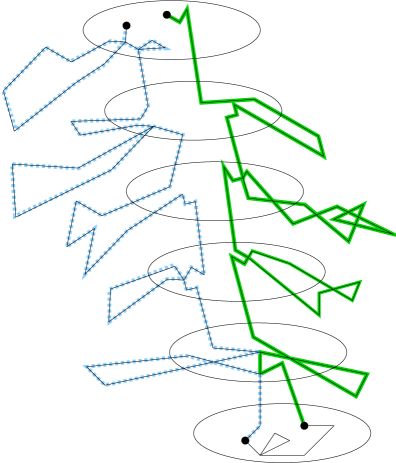
$\mathfrak{a}$ $\mathfrak{b}$ $\{o\}\times H$ $\{\tilde{z}\}\times H$ $\{z\}\times H$ $\pi_{\mathrm{there}}$ $\pi_{\mathrm{back}}$

Figure 1.1: Strategy of proof in $T_{n}\times H$. In this picture, $\pi_{\mathrm{there}}$ and $\pi_{\mathrm{back}}$ do not intersect each other inside $T_{n-2}$, hence we obtain $\tilde{z}\in S_{n-1}$ such that the $\mathsf{LERW}$ path from ${\mathfrak{a}}$ to ${\mathfrak{b}}$ intersects $\{\tilde{z}\}\times H$.

To guarantee (1), and also to help with (2), we will ensure that neither $\pi_{\mathrm{there}}$ nor $\pi_{\mathrm{back}}$ makes any backtracking on the ray of bags from $o$ to $z$, and furthermore, the bags that $\pi_{\mathrm{there}}$ enters outside this ray are different from the bags that $\pi_{\mathrm{back}}$ enters. See Figure 1.1. These requirements concern only the tree-coordinate of the random walk, and it is indeed possible to find $z$ such that they (and hence (1)) are satisfied, as we will prove in Proposition 2.1.

It remains to rule out intersections as in (2). Here the $H$-coordinates will play the main role. The intuition is that the visits in a typical bag $\{v\}\times H$ are not too long (since $k$ is large compared to $d$), and the places where the walker enters $\{v\}\times H$ from the outside are likely to be far from each other, because these entrances tend to be separated by long time intervals (until the walk on the tree returns) and because $H$ is large. To elaborate this argument will require some work, presented in Section 3.

For Theorem 1.2, the idea is to start with a small degree $d$ but large $H$ compared to $k$, so that Theorem 1.1 applies, then change the generating set so that we get the complete graph on $H$. This makes the random walk that generates the $\mathsf{LERW}$ spend a lot of time in each bag $\{v\}\times H$ before moving in the tree-coordinate, making it very likely that the loop-erasure erases every long excursion away from the root bag $\{o\}\times H$. The details are worked out in Section 4.

In Section 5, we prove Theorem 1.3 on lightness in the non-unimodular setting. Here the task is to modify the tree-proof to a well-chosen non-unimodular transitive graph, then argue that there are infinitely many components in the $\mathsf{FUSF}$, which makes at least some of them light.

We conclude the paper with several open problems in Section 6, including the ones on Gaboriau’s question and on our new graph parameter $\mathsf{disco}(H)$ for finite graphs $H$.

2 Born to be alive

A key observation about the tree-coordinate of the random walk will be the following proposition, somewhat interesting in its own right. Consider simple random walk $(Y_{t})_{t\geq 0}$ on $T_{n}$, started at the root $o$, until the first return time $\tau_{o}^{+}:=\min\{t>0:Y_{t}=o\}$.

Proposition 2.1 (Viable rays).

For any $k$ large enough, with a positive probability that may depend only on $k$, there is a $z\in S_{n}$ in $\mathbb{T}^{k}$ such that, denoting the ray from $o$ to $z$ in $T_{n}$ by $\gamma=(o=\gamma_{0},\gamma_{1},\dots,\gamma_{n}=z)$, we have:

• all the edges on the ray $\gamma$ are crossed exactly twice until $\tau_{o}^{+}$ (once on the way from $o$ to $z$, once on the way back);

• on the way from $o$ to $z$, for every $i=1,\dots,n-1$, the number of excursions away from $\gamma_{i}$ before taking the edge $(\gamma_{i},\gamma_{i+1})$ is at most $k/2$;

• denoting by $E_{i}$ and $F_{i}$ the set of edges incident to a vertex $\gamma_{i}$ but not on $\gamma$ that are crossed on the way to $z$, and on the way back from $z$ to $o$, respectively, we have that $E_{i}\cap F_{i}=\emptyset$ for all $i=1,\dots,n-1$.

Such a ray typically has the property that all its vertices have positive but small local times (of order $k$) until $\tau_{0}^{+}$. It is possible that, using the Dynkin isomorphism theorem [Dyn84], such a result could be proved via the Gaussian Free Field on $\mathbb{T}^{k}$; see [DLP12, Lup16, Zha18] for such arguments. However, since we also need the more refined statement on the edges incident to the ray, we have not tried to make this connection precise. Let us emphasize that a typical ray to $S_{n}$, or the first ray along which we reach $S_{n}$, do not satisfy the proposition; we have to work to find such rays.

Proof of Proposition 2.1. Pick a leaf $z\in S_{n}$, denote the ray from $o$ to $z$ by $\gamma=\gamma(z)$, the stopping times $\tau_{z}:=\min\{t:Y_{t}=z\}$ and $\tau^{+}_{o}$ as before, and define the events

$$\begin{aligned} \mathcal{A}_{z}&:=\Big{\{}\textrm{the edge }(\gamma_{i-1},\gamma_{i})\textrm{ is crossed exactly twice by }(Y_{t})_{t=0}^{\tau^{+}_{o}}\textrm{, for all }i=1,2,\dots,n\Big{\}},\\ \mathcal{L}_{z}&:=\Big{\{}\big{|}\big{\{}t\in\{1,\dots,\tau_{z}\}:Y_{t}=\gamma_{i}\big{\}}\big{|}\leq k/2+1\textrm{, for all }i=1,2,\dots,n\Big{\}}.\end{aligned}$$ (2.1)

Furthermore, let $E_{i}$ and $F_{i}$ be the set of edges as defined in Proposition 2.1, and define the event

$$\mathcal{B}_{z}:=\mathcal{A}_{z}\cap\mathcal{L}_{z}\cap\big{\{}E_{i}\cap F_{i}=\emptyset\textrm{ for all }i=1,2,\dots,n-1\big{\}}.$$ (2.2)

Let us calculate ${{\bf P}(\mathcal{B}_{z})}$. The first step has to be ${{\bf P}(Y_{1}=\gamma_{1})}=1/k$, and then, for each $\gamma_{i}$, $i=1,\dots,n-1$, the walk $(Y_{t})$ may take excursions away from $\gamma_{i}$, but it has to choose $\gamma_{i+1}$ before $\gamma_{i-1}$, and the number of excursions has to be at most $k/2$. The probability of this event $\mathsf{There}_{i}$, with the extra condition that there are precisely $j\geq 0$ excursions, is

$${{\bf P}\bigl{(}\mathsf{There}_{i},\textrm{ with }j\textrm{ excursions}\bigr{)}}=\left(1-\frac{2}{k}\right)^{j}\frac{2}{k}\,\frac{1}{2},$$ (2.3)

independently of what happens at other $\gamma_{i}$’s. When we arrive at $Y_{\tau_{z}}=z$, we have already sampled the edge sets $E_{i}$, $i=1,\dots,n-1$. Then, at each $\gamma_{i}$, for $i=n-1,n-2,\dots,1$, we have to choose $\gamma_{i-1}$ before $\gamma_{i+1}$, an event we will denote by $\mathsf{Back}_{i}$; furthermore, the excursions away from $\gamma_{i}$ have to produce an edge set $F_{i}$ that is disjoint from $E_{i}$. The probability of everything together, independently of $i$, is

$$p_{k}:={{\bf P}\bigl{(}\mathsf{There}_{i},\ \mathsf{Back}_{i},\textrm{ and }E_{i}\cap F_{i}=\emptyset\bigr{)}}\geq\sum_{j=0}^{\lfloor k/2\rfloor}\left(1-\frac{2}{k}\right)^{j}\frac{1}{k}\frac{1}{j+2}\asymp\frac{\log k}{k}\,,$$ (2.4)

because if we have $j\leq k/2$ excursions in (2.3), then $|E_{i}|\leq j$, thus the walk on the way back has to avoid at most $j+1$ neighbors before choosing $\gamma_{i-1}$ (the edges of $E_{i}$ plus the edge to $\gamma_{i+1}$), which has success probability $1$ in at most $j+2$ . The asymptotic formula at the end simply follows from the exponential factor being between 1 and $1/e$ for all $0\leq j\leq k/2$; the symbol $\asymp$ means “up to positive universal constant factors”, independently of $k$ or $n$.

The events of (2.4) for different $i$’s are independent from each other, hence we have

$${{\bf P}(\mathcal{B}_{z})}=\frac{1}{k}\,p_{k}^{n-1}.$$ (2.5)

Let $Z_{n}$ be the set of leafs $z\in S_{n}$ that satisfy the event $\mathcal{B}_{z}$. Then we have the first moment

$$\mathbb{E}|Z_{n}|=k(k-1)^{n-1}\,\frac{1}{k}\,p_{k}^{n-1},$$ (2.6)

which goes to infinity as $n\to\infty$ if $k$ is large enough, by (2.4).

To estimate the second moment $\mathbb{E}|Z_{n}|^{2}$, let $z,v\in S_{n}$ be leafs such that their last common ancestor is $w\in S_{m}$, with $m\geq 1$. We claim that

$${{\bf P}\bigl{(}\mathcal{B}_{z}\cap\mathcal{B}_{v}\bigr{)}}\asymp_{k}p_{k}^{2n-m}\,,$$ (2.7)

where $p_{k}$ is defined in (2.4), and $\asymp_{k}$ means “up to constant factors that may depend on $k$, but not on $n$ or $m$”.

Indeed, the first step in $(Y_{t})$ has to be towards $w$; then we have to reach $w$ without ever stepping backwards along the ray from $o$ to $w$; then we have to step towards $z$ or $v$ before stepping backwards towards $o$; then we have to reach the chosen leaf without backward moves; then we have to go back to $w$ without backward moves, and with the $F_{i}$ sets avoiding the $E_{i}$’s; at $w$, we have to step towards the other leaf before stepping towards $o$; if we define $F^{\prime}_{m}$ to be the set of edges emanating from $w$ that are crossed after reaching $w$ after the first leaf, but before the step towards the second leaf, we must have $E_{m}\cap F^{\prime}_{m}=\emptyset$; from $w$ we have to reach the other leaf without ever stepping backwards; then we have to go back to $w$, without backward moves, and with the $F_{i}$ sets avoiding the $E_{i}$’s also along this branch; at $w$, we have to move towards $o$ before moving towards $z$ or $v$ again, and the edge set $F^{\prime\prime}_{m}$ produced by the excursions before that has to be disjoint both from $E_{m}$ and $F^{\prime}_{m}$; then we have to reach $o$ without ever stepping backwards, again with the $F_{i}$ sets avoiding the $E_{i}$’s. We have $m-1+2(n-1-m)=2n-m-3$ of these conditions at vertices other than $w$, each with success probability $p_{k}$, independently from each other. At $w$, the conditions are obviously possible to satisfy if $k\geq 3$ (at the first visit go straight towards $z$, at the second visit go straight towards $w$, at the third visit go straight towards $o$), happening with probability at least $1/k^{3}$ and at most 1. So, the probability altogether is between $p_{k}^{2n-m-3}/k^{3}$ and $p_{k}^{2n-m-3}$, which can be written as (2.7).

By going through all possible last common ancestors $w$, from (2.7) we get

$$\mathbb{E}|Z_{n}|^{2}=\sum_{z,v\in S_{n}}{{\bf P}\bigl{(}\mathcal{B}_{z}\cap\mathcal{B}_{v}\bigr{)}}\asymp_{k}\sum_{m=1}^{n}k(k-1)^{m-1}\,(k-1)^{2(n-m)}\,p_{k}^{2n-m}\asymp_{k}\big{(}(k-1)p_{k}\big{)}^{2n}\,,$$ (2.8)

if $k$ is large enough, since $(k-1)p_{k}\to\infty$ holds by (2.4), hence the $m=1$ term will dominate.

Comparing (2.6) and (2.8), the Cauchy-Schwarz second moment method gives us

$${{\bf P}(|Z_{n}|>0)}\geq\frac{(\mathbb{E}|Z_{n}|)^{2}}{{\mathbb{E}(|Z_{n}|^{2})}}\asymp_{k}1,$$

finishing the proof of Proposition 2.1. ∎

3 Stayin’ alive

In this section, we will first recall how to generate the $\mathsf{FUSF}$ via an exhaustion by finite graphs and the loop-erased random walk $\mathsf{LERW}$ inside each finite graph. Then we will consider the random walk in $\mathbb{T}^{k}\times H$, together with its projection to $\mathbb{T}^{k}$, and show that some of the viable rays found in Section 2 correspond to trajectories in the product graph that survive the loop-erasure, provided that $H$ is large enough (compared to $k$). This way, we get distinct paths in the $\mathsf{FUSF}$ from two neighboring vertices to infinity.

As we briefly explained in the Introduction, the $\mathsf{FUSF}$ of an infinite graph $G$ is defined as the weak limit of the sequence $\mathsf{UST}(G_{n})$, where $(G_{n})_{n\geq 1}$ is any increasing sequence of connected finite subgraphs of $G$ such that $\bigcup_{n\geq 1}G_{n}=G$, and $\mathsf{UST}$ is the uniform measure on all spanning trees of the finite graph. The limit exists and is independent of the sequence $(G_{n})$ by some electric network monotonicity arguments [LP16, Chapter 10]. On a connected finite graph $G$, we can use the loop-erased random walk $\mathsf{LERW}$ to construct $\mathsf{UST}(G)$ with Wilson’s algorithm [Wil96]. Choose two vertices $x_{0},x_{1}$ of $G$, and produce a simple path from $x_{1}$ to $x_{0}$ by running a random walk from $x_{1}$ until hitting $x_{0}$, and erasing all cycles created by the trajectory, in the order of creation. Then pick some $x_{2}$, start a walk from $x_{2}$ until we hit the path between $x_{0}$ and $x_{1}$, take the loop-erasure of it, and so on, always walking from $x_{i}$ until we hit the already existing tree, repeating until all the vertices become part of the tree.

Our infinite graph will be a direct product $G=\mathbb{T}^{k}\times H$, often denoted by $\mathbb{T}^{k}\square H$, where the vertex set is just the set of pairs, and the neighbors of $(t,h)$ are the vertices $(t^{\prime},h)$ with $\{t,t^{\prime}\}\in E(\mathbb{T}^{k})$ and the vertices $(t,h^{\prime})$ with $\{h,h^{\prime}\}\in E(H)$.

Proof of Theorem 1.1. We take the exhaustion $G_{n}=T_{n}\times H$ of $G=\mathbb{T}^{k}\times H$. Our first step in Wilson’s algorithm is to take the loop-erased random walk $\mathsf{LERW}$ from ${\mathfrak{a}}=(o,h_{\mathfrak{a}})$ to ${\mathfrak{b}}=(o,h_{\mathfrak{b}})$, where $h_{\mathfrak{a}}\not=h_{\mathfrak{b}}\in H$ are arbitrary. We will prove that the $\mathsf{LERW}$ from $\mathfrak{a}$ to $\mathfrak{b}$, with a probability greater than a positive number $p$ that does not depend on $n$, will contain some close-to-the-boundary vertex $(\tilde{z},h_{\tilde{z}})\in S_{n-7}\times H$. Then, for any fixed finite subgraph $U$ of $G$, if $n$ is large enough so that $G_{n}$ contains $U$, but $S_{n-7}\times H$ is already disjoint from $U$, and the above event for the $\mathsf{UST}(G_{n})$-path between $\mathfrak{a}$ and $\mathfrak{b}$ occurs, then the intersection of this $\mathsf{UST}(G_{n})$-path with $U$ will not connect $\mathfrak{a}$ and $\mathfrak{b}$. Hence, in the weak limit as $n\to\infty$, the $\mathsf{FUSF}$-component of $\mathfrak{a}$ will be different from the component of $\mathfrak{b}$ with probability at least $p$.

One way to complete the proof from here is that the number of trees in the $\mathsf{FUSF}$ in any unimodular transitive graph was shown in [Tim18] and [HN17] to be either one a.s., or infinite a.s., hence we have to be now in the second case. We will also give a direct proof for our very special product graph, immediately extendable to the non-unimodular graph of Section 5, via Wilson’s algorithm, at the end of this section. And, we will give yet another proof, using the Mass Transport Principle, which again works both for unimodular and non-unimodular transitive graphs that are tree-like in some sense, and in a larger generality than the $\mathsf{FUSF}$, in Proposition 5.3. Some readers might prefer the more specific Wilson’s algorithm proof, some readers might prefer the more general MTP proof, but in any case, not relying on unimodularity will be important for Theorem 1.3.

We now turn to the study of the $\mathsf{LERW}$ from $\mathfrak{a}$ to $\mathfrak{b}$. The random walk on $G_{n}$ from $\mathfrak{a}$ to $\mathfrak{b}$ for which we apply the loop-erasure will be denoted by $(X_{t})_{t\geq 0}$. The first coordinate of $(X_{t})_{t\geq 0}$ is a lazy random walk on $T_{n}$, denoted by $(Y_{t})_{t\geq 0}$. As before, we fix $z\in S_{n}$, and let $\tau_{z}$ and $\tau^{+}_{o}$ denote the hitting times for the projection $(Y_{t})$. Condition on the event $\mathcal{B}_{z}$ of (2.2), but with the local times at $\gamma_{i}$ in the definition of $\mathcal{L}_{z}$ being understood as the number of “essentially different visits”, i.e., with the lazy steps removed from $(Y_{t})$. The last time before $\tau_{z}$ that $(X_{t})$ is in $\gamma_{i}\times H$ is denoted by $\alpha_{i}$, and the first time after $\tau_{z}$ that $(X_{t})$ is in $\gamma_{i}\times H$ is denoted by $\beta_{i}$. (For $i=n$, we mean $\alpha_{n}=\beta_{n}=\tau_{z}$.) Furthermore, the number of actual (non-lazy) steps until $\alpha_{i}$ in the $\mathbb{T}^{k}$ and $H$ coordinates will be denoted by $\alpha^{\mathbb{T}}_{i}$, $\alpha^{H}_{i}$, respectively, and similarly for $\beta_{i}$. The first ingredient in our proof will be that, with a uniformly positive probability, quite a long time passes between entering consecutive bags of $\gamma\times H$ during $\pi_{\mathrm{back}}$.

Lemma 3.1.

Let $\mathcal{F}(\beta_{i})$ be the sigma-algebra generated by $(X_{t})_{t=0}^{\beta_{i}}$. Then, for any $1\leq i\leq n-7$,

$${{\bf P}\bigl{(}\beta^{H}_{i-1}-\beta^{H}_{i}>k^{5}\bigm{|}\mathcal{B}_{z},\mathcal{F}(\beta_{i})\bigr{)}}>b$$

for any large enough $k$, with a constant $b>0$ that does not depend on $i$, $n$, or $k$.

Proof. Since we are conditioning on an event concerning the entire random walk trajectory, $\mathcal{B}_{z}$, we have to be careful what the exact effect of this is. Namely, for any such event $\mathcal{B}$, the original random walk transition probabilities get reweighted by a Bayesian factor:

$${{\bf P}\Bigl{(}X_{t+1}\Bigm{|}(X_{s})_{1\leq s\leq t},\mathcal{B}\Bigr{)}}={{\bf P}\bigl{(}X_{t+1}\bigm{|}(X_{s})_{1\leq s\leq t}\bigr{)}}\frac{{{\bf P}\bigl{(}\mathcal{B}\bigm{|}(X_{s})_{1\leq s\leq t+1}\bigr{)}}}{{{\bf P}\bigl{(}\mathcal{B}\bigm{|}(X_{s})_{1\leq s\leq t}\bigr{)}}}.$$ (3.1)

Now, for the lemma, it is enough to prove that

$${{\bf P}\bigl{(}\beta^{\mathbb{T}}_{i-1}-\beta^{\mathbb{T}}_{i}>2k^{6}\bigm{|}\mathcal{B}_{z},\mathcal{F}(\beta_{i})\bigr{)}}>b^{\prime},$$ (3.2)

with some constant $b^{\prime}>0$, by the following reasoning. Whenever $X_{t}\in\gamma_{i}\times H$ at some time $t\geq\beta_{i}$, the conditioning on $\mathcal{B}_{z}$ forbids the $\mathbb{T}^{k}$-steps through $(\gamma_{i},\gamma_{i+1})$ and $E_{i}$, while the other $\mathbb{T}^{k}$-steps and all the $H$-steps are available. In other words, the Bayesian factor from (3.1), with $\mathcal{B}=\mathcal{B}_{z}$ and also conditioned on $\mathcal{F}(\beta_{i})$, is zero for $X_{t+1}\in\gamma_{i+1}\times H$ and for $(X_{t},X_{t+1})\in E_{i}\times H$, while positive for other possible $X_{t+1}$’s. Namely, for the $H$-steps (i.e., for $X_{t+1}\in\gamma_{i}\times H$), the Bayesian factors are all $1$, since $\mathcal{B}_{z}$ depends only on the $\mathbb{T}^{k}$-coordinate, so its probability is the same starting from any vertex of $\gamma_{i}\times H$. For those $\mathbb{T}^{k}$-steps that are away from $\gamma$ and not excluded by $E_{i}$, the Bayesian factors are again $1$, because we will return to $\gamma_{i}\times H$ before making a step to $\gamma_{i\pm 1}\times H$. Finally, for the $\mathbb{T}^{k}$-step to $\gamma_{i-1}$ the Bayesian factor is at most $k$, by rearranging

$${{\bf P}\bigl{(}\mathcal{B}_{z}\bigm{|}X_{0},\dots,X_{t}=(\gamma_{i},h)\bigr{)}} \geq\frac{1}{d+k}{{\bf P}\bigl{(}\mathcal{B}_{z}\bigm{|}X_{0},\dots,X_{t}=(\gamma_{i},h),X_{t+1}=(\gamma_{i-1},h)\bigr{)}}$$

$$\qquad+\frac{d}{d+k}{{\bf P}\bigl{(}\mathcal{B}_{z}\bigm{|}X_{0},\dots,X_{t}=(\gamma_{i},h),X_{t+1}\in\gamma_{i}\times H)\bigr{)}},$$

which holds for any $t$ and any $h\in H$. Thus, the total weight of $H$-steps is $d$, while the total weight of $\mathbb{T}^{k}$-steps is at most $2k-1$, hence, before each $\mathbb{T}^{k}$-step, the number of $H$-steps stochastically dominates a $\mathsf{Geom}\big{(}(2k-1)/(2k-1+d)\big{)}-1$ variable. The stopping times $\alpha_{i}$ and $\beta_{i}$ are measurable with respect to the $\mathbb{T}^{k}$-coordinate of $(X_{t})$, hence conditioned on all the events of (3.2), i.e., on $\beta^{\mathbb{T}}_{i-1}-\beta^{\mathbb{T}}_{i}>2k^{6}$ and $\mathcal{B}_{z}$ and on $\mathcal{F}(\beta_{i})$, the variable $\beta^{H}_{i-1}-\beta^{H}_{i}$ stochastically dominates a sum of $2k^{6}$ iid variables with mean $d/(2k-1)$ and variance $d(2k-1+d)/(2k-1)^{2}$. Since $d\geq 2$, the expectation of the sum is larger than $2k^{5}$, and if $k$ is large enough, then the variance of the sum is less than $k^{6}$, hence the sum itself is larger than $k^{5}$ with a uniformly positive probability by Chebyshev’s inequality.

For a proof of (3.2), first notice that, given $\mathcal{B}_{z}$ and $\mathcal{F}(\beta_{i})$, the Bayesian factors calculated in the previous paragraph show that with a uniformly positive probability the step $(X_{\beta_{i}},X_{\beta_{i}+1})$ is in the $\mathbb{T}^{k}$-coordinate, away from $o$, into a branch different from $\gamma$ and $E_{i}$. (We are conditioning on the event $\mathcal{L}_{z}$ of (2.1) exactly in order for this uniformity to hold: the total Bayesian weight of these steps is at least $k/2-1$, while the total weight of all other steps is at most $k+d$.) From here, the distance of $(Y_{t})$ from $\gamma_{i}$ is a biased random walk: whenever it changes (the step is in the $\mathbb{T}^{k}$-coordinate), it decreases with probability $1/k$ and increases otherwise. So, it will reach level $S_{n}$ with a uniformly positive probability. After this, whenever the walk is at $S_{n-1}$, it reaches level $S_{i}$ before $S_{n}$ only with probability $\asymp(k-1)^{i-n+1}$, by the usual exponential martingale argument [Dur10, Theorem 5.7.7]. For $i\leq n-7$, this is at most $O(k^{-6})$. That is, the number of steps in the $\mathbb{T}^{k}$-coordinate until returning to $S_{i}$ from $S_{n-1}$ stochastically dominates a geometric random variable with success probability $\asymp k^{-6}$, and this is at least $2k^{6}$ with a uniformly positive probability. This gives (3.2). ∎

The second ingredient will be that, both in $\pi_{\mathrm{there}}$ and $\pi_{\mathrm{back}}$, the amount of time spent in each bag $\gamma_{i}\times H$ is probably not very large. Namely, let $A_{i}$ be the set of times until time $\alpha_{i}$ when $X_{t}$ is in $\gamma_{i}\times H$, and let $B_{i}$ be the analogous set of times from time $\beta_{i}$ until $\tau^{+}_{o}$. We let $H(A_{i})$ and $H(B_{i})$ be the set of vertices in $\gamma_{i}\times H$ visited at these times. Conditioned on $\mathcal{B}_{z}$, the time spent in $\gamma_{i}\times H$, for $1\leq i\leq n-1$, is stochastically dominated by a $\mathsf{Geom}\big{(}1/(k+d-1)\big{)}$ variable on the way to $z$ and by an independent copy on the way back to $o$, since the forward move along $\gamma$ is always available, the backward move is never, and the forward move always has the largest Bayesian factor from (3.1). The time spent in $\gamma_{n}\times H$ is $\mathsf{Geom}\big{(}1/(d+1)\big{)}$. So, letting $\mathcal{G}_{i}$ denote the sigma-algebra generated by all the trajectory pieces outside the subgraph $G_{i}$ spanned by $\gamma_{i}\times H$ and the subgraphs of $G\setminus(\gamma\times H)$ hanging from there, up to time-translations for each piece (so, without the information how many steps within $G_{i}$ are taken), we have that, for any small $\delta>0$, if $D$ is a large enough absolute constant, then, for $i=1,\dots,n$,

$$\begin{aligned} {{\bf P}\Bigl{(}|A_{i}|,|B_{i}|<Dk\Bigm{|}\mathcal{B}_{z},\mathcal{G}_{i}\Bigr{)}}&\geq{{\bf P}\Bigl{(}\mathsf{Geom}\big{(}1/(k+d-1)\big{)}<Dk\Bigr{)}}^{2}\\ &=\left(1-\left(1-\frac{1}{k+d-1}\right)^{Dk}\right)^{2}\\ &>1-\delta\,.\end{aligned}$$ (3.3)

Now, if we have $|A_{i-1}|,|B_{i-1}|<Dk$ and also the event $\{\beta^{H}_{i-1}-\beta^{H}_{i}>k^{5}\}$ of Lemma 3.1, then $t-s>k^{5}$ for all $s\in A_{i-1}$ and $t\in B_{i-1}$, and hence the following lemma will be relevant to achieving $H(A_{i-1})\cap H(B_{i-1})=\emptyset$.

Lemma 3.2.

In any $d$-regular finite graph $H$ on more than $k^{5/2}$ vertices, if $t>k^{5}$, and $x,y\in V(H)$ are arbitrary, then the simple random walk heat kernel satisfies ${{\bf P}(X_{t}=y\mid X_{0}=x)}<C_{d}k^{-5/2}$, with a constant $C_{d}<\infty$ that depends only on $d$.

Proof. This is basically a special case of [Lyo05, Lemma 3.6 in the arXiv version] or [MP05], with a few minor additional remarks.

In both references, the Markov chain is supposed to have a uniform laziness. So, we apply these results to the chain given by two consecutive steps on $H$. Since $H$ is $d$-regular, the probability of staying put in this chain is $1/d$. The stationary distribution is uniform. So, the references imply the on-diagonal bound ${{\bf P}(X_{2t}=x\mid X_{0}=x)}<C_{d}k^{-5/2}$ for all even times $2t>k^{5/2}$. We then get the same off-diagonal bound ${{\bf P}(X_{2t}=y\mid X_{0}=x)}<C_{d}k^{-5/2}$ by a standard Cauchy-Schwarz argument and the uniformity of the stationary distribution. Finally, to get the same bound for $X_{2t+1}$ being at $y$, average the bound over the neighbors of $y$ at time $2t$, before making the last step.

We also remark that to apply [MP05] one has to take $\epsilon=k^{-5/2}|H|$ there, which is not small (as suggested by the notation $\epsilon$), but that is actually not a requirement in that paper. ∎

If the trajectory $(X_{t})_{t=0}^{\tau^{+}_{o}}$ satisfies $\mathcal{B}_{z}$ and the intersection $\bigcap_{i=2}^{n-7}\big{\{}H(A_{i-1})\cap H(B_{i-1})=\emptyset\big{\}}$, then its loop-erasure will intersect $\gamma_{n-7}\times H$, implying the event that we are interested in. We will give an exponentially small lower bound on the probability of this event, with a base that does not depend on $k$.

First of all, let $\mathsf{Good}_{n-7}:=\bigcap_{i=1}^{n-8}\big{\{}|A_{i}|<Dk\big{\}}\in\mathcal{F}(\alpha_{n-8})$, and then iteratively, for $i\leq n-7$,

$$\mathsf{Prep}_{i-1} :=\mathsf{Good}_{i}\cap\big{\{}\beta^{H}_{i-1}-\beta^{H}_{i}>k^{5}\big{\}}\in\mathcal{F}(\beta_{i-1})\,,$$

$$\mathsf{Good}_{i-1} :=\mathsf{Prep}_{i-1}\cap\big{\{}H(A_{i-1})\cap H(B_{i-1})=\emptyset\big{\}}\in\mathcal{F}(\beta_{i-2})\,.$$

By (3.3), we have

$${{\bf P}\bigl{(}\mathsf{Good}_{n-7}\bigm{|}\mathcal{B}_{z}\bigr{)}}>(1-\delta)^{n-8}.$$ (3.4)

We will now give a lower bound on ${{\bf P}\bigl{(}\mathsf{Good}_{i-1}\bigm{|}\mathcal{B}_{z},\,\mathsf{Good}_{i}\bigr{)}}$, for each $2\leq i\leq n-7$.

First, consider $i=n-7$. By Lemma 3.1, we have ${{\bf P}\bigl{(}\mathsf{Prep}_{n-8}\bigm{|}\mathcal{B}_{z},\,\mathcal{F}(\beta_{n-7})\bigr{)}}>b$. Conditioned on $\mathcal{B}_{z}$ and $\mathcal{F}(\beta_{n-8})\cap\mathsf{Prep}_{n-8}$, the bound (3.3) gives that $|B_{n-8}|<Dk$ also holds with probability at least $1-\delta$. Finally, since the actual $H$-steps taken in the walk $(X_{t})_{t\geq 0}$ are independent of the $\mathbb{T}^{k}$-steps and of the number of $H$-steps, Lemma 3.2 gives

$${{\bf P}\Bigl{(}H(A_{n-8})\cap H(B_{n-8})\not=\emptyset\Bigm{|}\mathcal{B}_{z},\,\mathcal{F}(\beta_{n-8}),\,\mathsf{Prep}_{n-8},\,\big{\{}|B_{n-1}|<Dk\big{\}}\Bigr{)}}\\ <(Dk)^{2}C_{d}k^{-5/2}<\delta,$$

for our earlier small $\delta>0$, provided that $k$ is large enough. Altogether, we have

$${{\bf P}\Bigl{(}\mathsf{Good}_{n-8}\Bigm{|}\mathcal{B}_{z},\,\mathcal{F}(\beta_{n-8}),\,\mathsf{Good}_{n-7}\Bigr{)}}>(1-\delta)^{2}b,$$ (3.5)

finishing the first step of the induction. Also, note for future reference that we have proved, for every $i\leq n-8$, that

$${{\bf P}\Bigl{(}\mathsf{Good}_{i}\Bigm{|}\mathcal{B}_{z},\,\mathcal{F}(\beta_{i}),\,\mathsf{Prep}_{i}\Bigr{)}}>(1-\delta)^{2}>1-2\delta.$$ (3.6)

The complication for the general $i\leq n-8$ step to get from $\mathsf{Good}_{i}$ to $\mathsf{Good}_{i-1}$ will be that the event $\big{\{}H(A_{i-1})\cap H(B_{i-1})=\emptyset\big{\}}\supset\mathsf{Good}_{i-1}$ concerns the trajectory from $\beta_{i-1}$ till $\beta_{i-2}$, hence interferes with the “future” event $\big{\{}\beta^{H}_{i-2}-\beta^{H}_{i-1}>k^{5}\big{\}}\supset\mathsf{Prep}_{i-2}$.

Now fix any $i\leq n-8$. We use Lemma 3.1 to get

$${{\bf P}\bigl{(}\mathsf{Prep}_{i-1}\bigm{|}\mathcal{B}_{z},\,\mathcal{F}(\beta_{i}),\,\mathsf{Good}_{i}\bigr{)}} >{{\bf P}\bigl{(}\mathsf{Prep}_{i-1}\bigm{|}\mathcal{B}_{z},\,\mathcal{F}(\beta_{i}),\,\mathsf{Prep}_{i}\bigr{)}}-{{\bf P}\bigl{(}\mathsf{Good}_{i}^{c}\bigm{|}\mathcal{B}_{z},\,\mathcal{F}(\beta_{i}),\,\mathsf{Prep}_{i}\bigr{)}}$$

$$>b-2\delta,$$ (3.7)

where the upper bound $2\delta$ is from (3.6). If we set $\delta:=b/4\leq 1/4$, then this lower bound becomes $b/2>0$, and it makes sense to continue as follows:

$${{\bf P}\bigl{(}\mathsf{Good}_{i-1}\bigm{|}\mathcal{B}_{z},\,\mathcal{F}(\beta_{i}),\,\mathsf{Good}_{i},\,\mathsf{Prep}_{i-1}\bigr{)}}$$

$$\hskip-72.26999pt>{{\bf P}\bigl{(}\mathsf{Good}_{i-1}\bigm{|}\mathcal{B}_{z},\,\mathcal{F}(\beta_{i}),\,\mathsf{Prep}_{i-1}\bigr{)}}-{{\bf P}\bigl{(}\mathsf{Good}_{i}^{c}\bigm{|}\mathcal{B}_{z},\,\mathcal{F}(\beta_{i}),\,\mathsf{Prep}_{i-1}\bigr{)}}$$

$$\hskip-72.26999pt>(1-\delta)^{2}-\frac{{{\bf P}\bigl{(}\mathsf{Good}_{i}^{c}\bigm{|}\mathcal{B}_{z},\,\mathcal{F}(\beta_{i}),\,\mathsf{Prep}_{i}\bigr{)}}}{{{\bf P}\bigl{(}\mathsf{Prep}_{i-1}\bigm{|}\mathcal{B}_{z},\,\mathcal{F}(\beta_{i}),\,\mathsf{Prep}_{i}\bigr{)}}}$$

$$\hskip-72.26999pt\geq(1-\delta)^{2}-\frac{2\delta}{b}\geq\frac{9}{16}-\frac{1}{2}=\frac{1}{16}.$$ (3.8)

The estimates (3.7) and (3.8) together give

$${{\bf P}\bigl{(}\mathsf{Good}_{i-1}\bigm{|}\mathcal{B}_{z},\,\mathcal{F}(\beta_{i}),\,\mathsf{Good}_{i}\bigr{)}}>\frac{b}{32},$$ (3.9)

for $2\leq i\leq n-8$. Telescoping this with (3.4) and (3.5), we get

$${{\bf P}\Bigl{(}\bigcap_{i=2}^{n-7}\big{\{}H(A_{i-1})\cap H(B_{i-1})=\emptyset\big{\}}\Bigm{|}\mathcal{B}_{z}\Bigr{)}}\geq{{\bf P}\Bigl{(}\bigcap_{i=1}^{n-7}\mathsf{Good}_{i}\Bigm{|}\mathcal{B}_{z}\Bigr{)}}\geq\left(\frac{3}{4}\right)^{n-8}\frac{9b}{16}\left(\frac{b}{32}\right)^{n-9}.$$ (3.10)

From this exponentially small lower bound, to find a good $z\in S_{n}$ and hence a good $\tilde{z}\in S_{n-7}$ with a uniformly positive probability, we will again use the second moment method, for which we need a little bit of preparation. Define the events

$$\mathcal{C}_{z} :=\mathcal{B}_{z}\cap\big{\{}H(A_{i})\cap H(B_{i})=\emptyset\textrm{ for all }i=1,\dots,n-8\big{\}},$$

$$\mathcal{C}_{z}(h) :=\mathcal{C}_{z}\cap\{X_{\tau^{+}_{o}}=(o,h)\},\quad h\in H.$$

Then, as (3.10) says,

$${{\bf P}\bigl{(}\mathcal{C}_{z}\bigm{|}\mathcal{B}_{z}\bigr{)}}>\frac{9}{16}\left(\frac{3b}{128}\right)^{n-8}.$$ (3.11)

Furthermore, we claim that

$$\max_{h\in H}{{\bf P}\bigl{(}\mathcal{C}_{z}(h)\bigm{|}\mathcal{B}_{z}\bigr{)}}\leq C\min_{h\in H}{{\bf P}\bigl{(}\mathcal{C}_{z}(h)\bigm{|}\mathcal{B}_{z}\bigr{)}},$$ (3.12)

with a constant $C<\infty$ that may depend on $H$ and $k$, but not on $n$.

In the proof of this claim, we will use a small technical lemma:

Lemma 3.3.

Every finite transitive graph $H$ is 2-vertex-connected: for any vertex $g\in V(H)$, the graph we get from $H$ by deleting $g$ is still connected.

Proof. Assume that there is a cut-vertex $g$, whose removal cuts $H$ into at least two components; denote the largest of these by $H_{g}$ (or one of the largest ones in case of a draw). Take some vertex $h$ not in $\{g\}\cup H_{g}$. By transitivity, $h$ is also a cut-vertex, whose removal results in at least two components, one containing both $g$ and $H_{g}$. But this component will have a size strictly larger than $|H_{g}|$, contradicting transitivity.∎

To prove (3.12), first observe that, if we condition the random walk trajectory $(X_{t})$ to satisfy $\mathcal{C}_{z}$, and let $X_{\alpha_{3}}=(\gamma_{3},h_{\mathrm{out}})$ be the last vertex in $\gamma_{3}\times H$ on the trajectory before $\tau_{z}$, and let $X_{\beta_{3}}=(\gamma_{3},h_{\mathrm{in}})$ be the first one after $\tau_{z}$, then, conditionally on $h_{\mathrm{out}}$ and $h_{\mathrm{in}}$, the part of the trajectory between $h_{\mathrm{out}}$ and $h_{\mathrm{in}}$ is independent of the rest. Therefore, if we prove that there exists some $p>0$, depending only on $H$ and $k$, but not on $n$, such that, for any two vertices $h_{\mathrm{out}}\not=h_{\mathrm{in}}$, and any $h\in H$, the probability that $(X_{t})_{t=0}^{\alpha_{3}}$ and $(X_{t})_{t=\beta_{3}}^{\tau^{+}_{o}}$ satisfy the conditions of $\mathcal{C}_{z}(h)$ relating to $\gamma_{i}\times H$ for $i=0,1,2,3$ is at least $p$, then $C=1/p$ will clearly work in (3.12). For the argument that follows, see Figure 3.1.

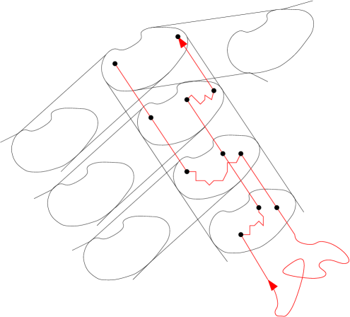
$o=\gamma_{0}$ $\gamma_{1}$ $\gamma_{2}$ $\gamma_{3}$ $h_{\mathfrak{a}}$ $h$ $h^{\prime}$ $h^{\prime}$ $h_{\textrm{in}}$ $h_{\textrm{out}}$ ${\color[rgb]{1,0,0}\pi_{\textrm{in}}}$ ${\color[rgb]{1,0,0}\pi_{\textrm{out}}}$ ${\color[rgb]{1,0,0}\pi_{h}}$

Figure 3.1: Producing a good random walk trajectory in $\mathbb{T}^{k}\times H$.

Pick any vertex $h^{\prime}\in H\setminus\{h_{\mathrm{out}},h_{\mathfrak{a}}\}$. By the 2-connectedness of $H$, we can pick a path $\pi_{\mathrm{in}}$ in $\gamma_{3}\times H$ between $(\gamma_{3},h_{\mathrm{in}})$ and $(\gamma_{3},h^{\prime})$ that avoids $(\gamma_{3},h_{\mathrm{out}})$, a path $\pi_{\mathrm{out}}$ in $\gamma_{2}\times H$ between $(\gamma_{2},h_{\mathrm{out}})$ and $(\gamma_{2},h_{\mathfrak{a}})$ that avoids $(\gamma_{2},h^{\prime})$, and a path $\pi_{h}$ in $\gamma_{1}\times H$ between $(\gamma_{1},h)$ and $(\gamma_{1},h^{\prime})$ that avoids $(\gamma_{1},h_{\mathfrak{a}})$. Then $(X_{t})_{t=0}^{\alpha_{3}}$ can go from $(\gamma_{0},h_{\mathfrak{a}})$ straight to $(\gamma_{2},h_{\mathfrak{a}})$, then to $(\gamma_{2},h_{\mathrm{out}})$ via $\pi_{\mathrm{out}}$, then straight to $(\gamma_{3},h_{\mathrm{out}})$, and $(X_{t})_{t=\beta_{3}}^{\tau^{+}_{o}}$ can go from $(\gamma_{3},h_{\mathrm{in}})$ via $\pi_{\mathrm{in}}$ and $\pi_{h}$ to $(\gamma_{0},h)$. All of this happens with probability at least $(d+k)^{-3|H|-6}$, which proves (3.12). (Note that we needed the extra vertex $h^{\prime}$ and the four layers $\gamma_{0},\dots,\gamma_{3}$ for this construction because it might happen that $h=h_{\mathrm{out}}$; otherwise, taking $h^{\prime}:=h$ and removing the $\gamma_{1}$ layer could have worked.)

We are now ready for the second moment method. Let $W_{n}$ be the set of leaves $z\in S_{n}$ that satisfy $\mathcal{C}_{z}(h_{\mathfrak{b}})$, with the desired endpoint $\mathfrak{b}=(o,h_{\mathfrak{b}})$. We will run a second moment argument, as in Section 2, to show that $W_{n}$ is non-empty with a positive probability, uniformly in $n$.

First note that (3.11) and (3.12) imply

$$q(n):={{\bf P}\bigl{(}\mathcal{C}_{z}(h_{\mathfrak{b}})\bigm{|}\mathcal{B}_{z}\bigr{)}}>c\,\left(\frac{3b}{128}\right)^{n},$$ (3.13)

where $c$ depends on $H$ and $k$, but not on $n$. Together with (2.5), we have

$$\mathbb{E}|W_{n}|\,\asymp_{k,H}\,(k-1)^{n}\,p_{k}^{n}\,q(n).$$ (3.14)

Using (2.4) and (3.13), this tends to infinity as $n\to\infty$ for $k$ large enough.

To estimate the second moment ${\mathbb{E}\bigl{(}|W_{n}|^{2}\bigr{)}}$, let $z,v\in S_{n}$ be leafs such that their last common ancestor is $w\in S_{m}$, with $m\geq 1$. We claim that

$${{\bf P}\bigl{(}\mathcal{C}_{z}(h_{\mathfrak{b}})\cap\mathcal{C}_{v}(h_{\mathfrak{b}})\bigm{|}\mathcal{B}_{z}\cap\mathcal{B}_{v}\bigr{)}}\leq Q\,q(n)\,q(n-m),$$ (3.15)

with some $Q<\infty$ that depends only on $H$ and $k$, but not on $n$.

First note that we may assume that $m\leq n-10$, since otherwise the factor $q(n-m)$ on the right hand side of (3.15) is obviously at least a positive constant that does not depend on $n$, hence a suitable $Q$ does exist.

By symmetry, we may assume $\tau_{z}<\tau_{v}$. We first show that

$${{\bf P}\bigl{(}\mathcal{C}_{z}(h_{\mathfrak{b}})\bigm{|}\mathcal{B}_{z}\cap\mathcal{B}_{v}\cap\{\tau_{z}<\tau_{v}\}\bigr{)}}\leq C_{k,H}\,{{\bf P}\bigl{(}\mathcal{C}_{z}(h_{\mathfrak{b}})\bigm{|}\mathcal{B}_{z}\bigr{)}}.$$ (3.16)

We do this by coupling (with a uniformly positive probability) the trajectory $(X_{t})$ conditioned on $\mathcal{B}_{z}$ to be identical to the trajectory conditioned on $\mathcal{B}_{z}\cap\mathcal{B}_{v}\cap\{\tau_{z}<\tau_{v}\}$, denoted by $(\tilde{X}_{t})$, within the ray $\gamma\times H$ (which leads from $o$ to $z$), except for a bounded neighborhood of $w=\gamma_{m}$. Given $\mathcal{B}_{z}$, we know from (3.9) that $H(A_{m})\cap H(B_{m})=\emptyset$ occurs with a uniformly positive probability, say $c_{1}>0$. Conditioning on $\mathcal{B}_{z}\cap\{H(A_{m})\cap H(B_{m})=\emptyset\}$ gives a certain distribution to the pairs of vertices $\big{(}X_{\alpha_{m-1}},X_{\beta_{m-1}}\big{)}$ and $\big{(}X_{\alpha_{m}},X_{\beta_{m}}\big{)}$, which are basically the places where the trajectory leaves $w\times H$. On the other hand, conditioning on $\mathcal{B}_{z}\cap\mathcal{B}_{v}\cap\{\tau_{z}<\tau_{v}\}$, we get some distribution on $(\tilde{X}_{t})_{t=\alpha_{m-4}}^{\alpha_{m+3}}$ and $(\tilde{X}_{t})_{t=\beta_{m+3}}^{\beta_{m-4}}$. Whenever these pieces of $(\tilde{X}_{t})$-trajectories satisfy $H(A_{i})\cap H(B_{i})=\emptyset$ for $i=m-3,\dots,m+3$ (so that $(\tilde{X}_{t})$ still has a chance to satisfy $\mathcal{C}_{z}(h_{\mathfrak{b}})$), the argument of Figure 3.1 gives that, conditioned on these trajectory pieces, with a probability at least $c_{2}>0$ that depends only on $k$ and $H$, we have that $(X_{t})_{t=\alpha_{m-4}}^{\alpha_{m+3}}$ and $(X_{t})_{t=\beta_{m+3}}^{\beta_{m-4}}$ satisfy $\big{(}X_{\alpha_{m+3}},X_{\beta_{m+3}}\big{)}=\big{(}\tilde{X}_{\alpha_{m+3}},\tilde{X}_{\beta_{m+3}}\big{)}$ and $\big{(}X_{\alpha_{m-4}},X_{\beta_{m-4}}\big{)}=\big{(}\tilde{X}_{\alpha_{m-4}},\tilde{X}_{\beta_{m-4}}\big{)}$. Conditioned on these equalities, we can couple the trajectories $(X_{t})_{t=0}^{\alpha_{m-4}}$, $(X_{t})_{t=\alpha_{m+3}}^{\beta_{m+3}}$, and $(X_{t})_{t=\beta_{m-4}}^{\tau_{o}^{+}}$ to be equal to the tilde versions, hence if $(\tilde{X}_{t})$ satisfies $\mathcal{C}_{z}(h_{\mathfrak{b}})$, so does $(X_{t})$. Altogether, (3.16) follows with $C_{k,H}=1/(c_{1}c_{2})$.

Now let $H(A_{m}),H(B^{\prime}_{m}),H(B^{\prime\prime}_{m})$ be the set of vertices in $w\times H$ visited before $\tau_{z}$, between $\tau_{z}$ and $\tau_{v}$, and after $\tau_{v}$, respectively; thus $H(B^{\prime}_{m})\cup H(B^{\prime\prime}_{m})=H(B_{m})$. Notice that $\mathcal{C}_{z}(h_{\mathfrak{b}})\cap\mathcal{C}_{v}(h_{\mathfrak{b}})$ implies that $H(A_{m}),H(B^{\prime}_{m}),H(B^{\prime\prime}_{m})$ are mutually disjoint, an event we will denote by $\mathcal{M}_{w}$. Condition now, beyond $\mathcal{B}_{z}\cap\mathcal{B}_{v}\cap\{\tau_{z}<\tau_{v}\}$, also on the event $\mathcal{C}_{z}(h_{\mathfrak{b}})\cap\mathcal{M}_{w}$. Let $h^{\prime}$ be the vertex in $H(B^{\prime}_{m})$ last visited before $\tau_{v}$, and let $h^{\prime\prime}$ be the first vertex in $H(B^{\prime\prime}_{m})$ after $\tau_{v}$. Since $H$ is transitive, there is an automorphism taking $h^{\prime}$ to $h_{\mathfrak{a}}$, and $h^{\prime\prime}$ to some $h^{*}$. Now, the events along the ray from $w$ to $v$ that are needed for $\mathcal{C}_{v}(h_{\mathfrak{b}})$ are just the events for some length $n-m$ ray, with the extra condition that the first step from $(w,h_{\mathfrak{a}})$ and the last step to $(w,h^{*})$ are both in the $\mathbb{T}^{k}$-coordinate. Thus, using (3.12), we have

$${{\bf P}\Bigl{(}\mathcal{C}_{v}(h_{\mathfrak{b}})\Bigm{|}\mathcal{C}_{z}(h_{\mathfrak{b}})\cap\mathcal{M}_{w}\cap\mathcal{B}_{z}\cap\mathcal{B}_{v}\cap\{\tau_{z}<\tau_{v}\}\Bigr{)}}<C^{\prime}_{k,H}\,q(n-m).$$ (3.17)

Since $\mathcal{M}_{w}\supset\mathcal{C}_{z}(h_{\mathfrak{b}})\cap\mathcal{C}_{v}(h_{\mathfrak{b}})$, we can combine this with

$${{\bf P}\bigl{(}\mathcal{C}_{z}(h_{\mathfrak{b}})\cap\mathcal{M}_{w}\bigm{|}\mathcal{B}_{z}\cap\mathcal{B}_{v}\cap\{\tau_{z}<\tau_{v}\}\bigr{)}}\leq C_{k,H}\,q(n),$$

which we get from (3.16), and we arrive at (3.15).

From (3.15) and (2.7), similarly to (2.8), we have

$$\mathbb{E}|W_{n}|^{2}\leq Q^{\prime}\sum_{m=1}^{n}k(k-1)^{m-1}\,(k-1)^{2(n-m)}\,p_{k}^{2n-m}\,q(n)\,q(n-m).$$ (3.18)

For the Cauchy-Schwarz second moment method, we want that $\mathbb{E}|W_{n}|^{2}<Q^{\prime\prime}(\mathbb{E}|W_{n}|)^{2}$, for some $Q^{\prime\prime}<\infty$ that does not depend on $n$. Substituting (3.14) and (3.18) into this inequality, then rearranging, we arrive at the following inequality to prove:

$$\sum_{m=1}^{n}\big{(}(k-1)p_{k}\big{)}^{-m}\,q(n-m)\stackrel{{\scriptstyle?}}{{<}}Q^{\prime\prime\prime}\,q(n).$$ (3.19)

The final ingredient is that, writing $y$ for vertex $\gamma_{m}$ on the ray from $o$ to $z$, again only for $m\leq n-10$, and writing $\mathcal{B}_{z}^{y}$ and $\mathcal{C}_{z}^{y}$ for the analogs of the events $\mathcal{B}_{z}=\mathcal{B}_{z}^{o}$ and $\mathcal{C}_{z}=\mathcal{C}_{z}^{o}$ when the root is $y$ instead of $o$,

$$\frac{q(n)}{q(n-m)}=\frac{{{\bf P}(\mathcal{C}_{z}^{o}(h_{\mathfrak{b}})\mid\mathcal{B}_{z}^{o})}}{{{\bf P}(\mathcal{C}_{z}^{y}(h_{\mathfrak{b}})\mid\mathcal{B}_{z}^{y})}} \asymp_{k,H}\frac{{{\bf P}\bigl{(}H(A_{i})\cap H(B_{i})=\emptyset\textrm{ for }i=1,2,\dots,n-8\bigm{|}\mathcal{B}_{z}^{o}\bigr{)}}}{{{\bf P}\bigl{(}H(A_{i})\cap H(B_{i})=\emptyset\textrm{ for }i=m+1,m+2,\dots,n-8\bigm{|}\mathcal{B}_{z}^{y}\bigr{)}}}$$

$$\asymp_{k,H}\frac{{{\bf P}\bigl{(}H(A_{i})\cap H(B_{i})=\emptyset\textrm{ for }i=1,2,\dots,n-8\bigm{|}\mathcal{B}_{z}^{o}\bigr{)}}}{{{\bf P}\bigl{(}H(A_{i})\cap H(B_{i})=\emptyset\textrm{ for }i=m+1,m+2,\dots,n-8\bigm{|}\mathcal{B}_{z}^{o}\bigr{)}}}$$

$$={{\bf P}\bigl{(}\mathcal{C}_{z}^{o}\bigm{|}\mathcal{B}_{z}^{o},\ H(A_{i})\cap H(B_{i})=\emptyset\textrm{ for }i=m+1,m+2,\dots,n-8\bigr{)}}$$

$$>(3b/128)^{m},$$

where the first $\asymp$ is by (3.12); the second $\asymp$ is by a coupling argument similar to the one that gave (3.16), now doing the coupling in $\{\gamma_{m},\dots,\gamma_{m+3}\}\times H$; and the inequality in the last line follows from (3.4) and (3.9), just like in (3.10). Plugging this into (3.19), we arrive at

$$\sum_{m=1}^{n}\big{(}(k-1)p_{k}\big{)}^{-m}(2/bg)^{m}\stackrel{{\scriptstyle?}}{{<}}Q^{\prime\prime\prime\prime},$$

which is true if $k$ is large enough, since (2.4) tells us that $(k-1)p_{k}\to\infty$ as $k\to\infty$. This finishes the proof of the disconnectedness Theorem 1.1. ∎

For the first direct proof of having infinitely many trees almost surely, pick an infinite ray $o_{1},o_{2},\dots$ in $\mathbb{T}^{k}$, pick any $h\in H$, and let $\mathfrak{a}_{i}:=(o_{i},h)$. Our exhaustion $G_{n}=T_{n}\times H$ contains $\mathfrak{a}_{1},\dots,\mathfrak{a}_{n}$. Perform Wilson’s algorithm in $G_{n}$ as follows.

First run a $\mathsf{LERW}$ from $\mathfrak{a}_{2}$ to $\mathfrak{a}_{1}$, denoted by $\ell_{1}$. By a small modification of our previous proof, with a positive probability that depends only on $H$ and $k$, this $\ell_{1}$ will first enter the subtree (times $H$) that starts at $o_{2}$ and does not contain $o_{1}$ or $o_{3}$, then will hit the boundary $S_{n}\times H$, then hits $o_{2}\times H$ at a vertex $\mathfrak{b}_{2}=(o_{2},h_{2})$ different from $\mathfrak{a}_{2}$, then goes straight to $(o_{1},h_{2})$, then hits $\mathfrak{a}_{1}=(o_{1},h)$ without leaving $o_{1}\times H$. Without conditioning on this good event, denoted by $\mathcal{G}_{1}$ hereafter, the $\mathbb{T}^{k}$-coordinate of the random walk that gives $\ell_{1}$, viewed only at the times when it moves on the ray $o_{1},\dots,o_{n}$, performs a simple random walk on this segment until $\tau^{+}_{o}$. The maximum $j$ for which $o_{j}$ is touched by the projection is stochastically dominated by the maximum of a one-dimensional random walk excursion, which is almost surely finite, since the walk is recurrent. The maximum $j$ for which $o_{j}\times H$ is touched by $\ell_{1}$, denoted by $j_{2}$, is even smaller. Let $\mathfrak{b}_{2}=(o_{j_{2}},h_{2})$ be the last vertex in $j_{2}\times H$ touched by $\ell_{1}$. Note that this definition of $\mathfrak{b}_{2}$ extends our previous one that we made under $\mathcal{G}_{1}$.

Next, run a $\mathsf{LERW}$ from $\mathfrak{a}_{j_{2}+1}$ to $\mathfrak{b}_{2}$, denoted by $\ell_{2}$, which, with a positive probability that depends only on $H$ and $k$, will enter the subtree (times $H$) that starts at $o_{j_{2}+1}$ and does not contain $o_{j_{2}}$ or $o_{j_{2}+2}$, then will hit the boundary of $T_{n}\times H$, then hits $o_{j_{2}+1}\times H$ at a vertex $\mathfrak{b}_{3}=(o_{j_{2}+1},h_{3})$ different from $\mathfrak{a}_{j_{2}+1}$, then goes straight to $(o_{j_{2}},h_{3})$, then hits $\mathfrak{b}_{2}$ without leaving $o_{j_{2}}\times H$. Without conditioning on this good event, denoted by $\mathcal{G}_{2}$, the maximum $j$ for which $o_{j}\times H$ is touched by $\ell_{2}$, denoted by $j_{3}$, has the property that $j_{3}-j_{2}$ is stochastically dominated by the maximum of a one-dimensional simple random walk excursion. Let $\mathfrak{b}_{3}=(o_{j_{3}},h_{3})$ be the last vertex in $j_{3}\times H$ touched by $\ell_{2}$, extending the definition that we made under $\mathcal{G}_{2}$.

Iterate this procedure until we have reached $o_{n}\times H$, producing the $\mathsf{LERW}$ paths $\ell_{1},\dots,\ell_{I_{n}}$. Since the distribution of $j_{i+1}-j_{i}$ is always stochastically dominated by the maximum of a one-dimensional simple random walk excursion, the variable $I_{n}$ tends to infinity in probability, as $n\to\infty$. Each $\ell_{i}$, independently of the previous ones, satisfies $\mathcal{G}_{i}$ with a positive probability that depends only on $H$ and $k$. Thus, the number of events $\mathcal{G}_{i}$ satisfied also tends to infinity in probability. This shows that the number of trees in the weak limit is almost surely infinite.

4 You can’t hide from yourself

Proof of Theorem 1.2. The natural free generating set in each coordinate of the product, together with their inverses, gives a tree $\mathbb{T}^{2k}$ in the $\mathbb{F}_{k}$ coordinate and a cycle in the $H=\mathbb{Z}_{k^{9}}$ coordinate (every edge that appears does so in both orientations, so, as usual, we consider them to be unoriented single edges). If $k$ is large enough, then Theorem 1.1 tells us that the $\mathsf{FUSF}$ has infinitely many trees almost surely.

The second Cayley graph will also be a direct product graph: we again take free generators for $\mathbb{F}_{k}$ with their inverses, while all the elements in $H=\mathbb{Z}_{k^{9}}$, except for the identity. This gives the Cayley graph $\mathbb{T}^{2k}\times K_{k^{9}}$, where $K_{n}$ is the complete graph on $n$ vertices with a single unoriented edge between any pair of vertices.

We will show that, for the $\mathsf{LERW}$ from ${\mathfrak{a}}=(o,h_{\mathfrak{a}})$ to ${\mathfrak{b}}=(o,h_{\mathfrak{b}})$, with $h_{\mathfrak{a}}\not=h_{\mathfrak{b}}\in H$, the probability that the $\mathsf{LERW}$ is not contained in $T_{r}\times H$ is exponentially small in $r$, if $k$ is large enough. (As before, $T_{r}$ is the ball of radius $r$ in $\mathbb{T}^{2k}$.) This of course implies the theorem.

Fix any ray $o=\gamma_{0},\gamma_{1},\dots,\gamma_{r}$ in $T_{r}$, and let $\beta_{r}$ be the last time that the simple random walk $(X_{t})_{t=0}^{\tau_{\mathfrak{b}}}$ from ${\mathfrak{a}}$ to ${\mathfrak{b}}$ enters the bag $\{\gamma_{r}\}\times H$ (i.e., the last $\beta$ such that $X_{\beta}\in\{\gamma_{r}\}\times H$ but $X_{\beta-1}\not\in\{\gamma_{r}\}\times H$). If the walk never enters $\{\gamma_{r}\}\times H$, we set $\beta_{r}=\infty$. If $\beta_{r}<\infty$, then we also let $\beta_{i}$, for $i=0,1,\dots,r-1$, be the last time before $\beta_{r}$ that $(X_{t})_{t\geq 0}$ enters the bag $\{\gamma_{i}\}\times H$, and let $\kappa_{i}$ be the first time after $\beta_{i}$ that $(X_{t})_{t\geq 0}$ is not in $\{\gamma_{i}\}\times H$ (in fact, because of $\beta_{r}<\infty$, we have $X_{\kappa_{i}}\in\{\gamma_{i+1}\}\times H$). Furthermore, we let $\mathsf{LERW}_{t}$ denote the loop-erasure of $(X_{s})_{s=0}^{t}$, and, still assuming $\beta_{r}<\infty$, we let $\alpha_{i}$ be the first time $\alpha$ with the property that $X_{\alpha}\in\{\gamma_{i}\}\times H$ and $\mathsf{LERW}_{\alpha}\cap\{X_{s}\}_{s=\alpha}^{\beta_{i}}=\{X_{\alpha}\}$. In other words, $X_{\alpha_{i}}$ is the first vertex along $\mathsf{LERW}_{\beta_{i}}$ that is in $\{\gamma_{i}\}\times H$. See Figure 4.1.

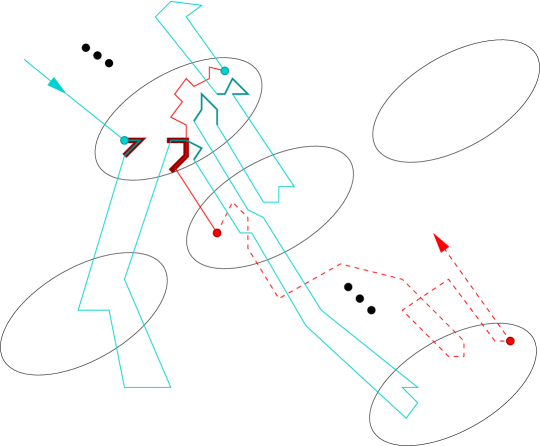
$\{\gamma_{i}\}\times H$ $\{\gamma_{r}\}\times H$ $X_{\alpha_{i}}$ $X_{\beta_{i}}$ $X_{\kappa_{i}}$ $X_{\beta_{r}}$

Figure 4.1: The cyan-colored path is $\mathsf{LERW}_{\beta_{i}}$. Its darker cyan parts are $\mathsf{LERW}_{\beta_{i}}\cap(\{\gamma_{i}\}\times H)$. The solid red path is $(X_{t})_{t=\beta_{i}}^{\kappa_{i}}$, the dashed red path is $(X_{t})_{t\geq\kappa_{i}}$ and the thick dark red pieces form $\mathsf{LERW}_{\kappa_{i}}\cap(\{\gamma_{i}\}\times H)$.

We will show that, with very high probability conditionally on $\beta_{r}<\infty$, for most $i=0,1,\dots,r$ the intersection $\mathsf{LERW}_{\kappa_{i}}\cap(\{\gamma_{i}\}\times H)$ is quite large. This will imply, introducing the notation $\varphi_{i}$ for the first time when the simple random walk from $\beta_{r}$ to $\tau_{\mathfrak{b}}$ enters $\{\gamma_{i}\}\times H$ again, and $\psi_{i}$ for the first time after $\varphi_{i}$ when the simple random walk is in $\{\gamma_{i\pm 1}\}\times H$, that the event

$$\mathsf{Avoid}_{i}:=\{\beta_{r}<\infty\}\cap\left\{\mathsf{LERW}_{\kappa_{i}}\cap(X_{t})_{t=\varphi_{i}}^{\psi_{i}}=\emptyset\right\}$$ (4.1)

is very unlikely to happen; in fact, we will show that

$${{\bf P}\Bigl{(}\bigcap_{i=1}^{r-1}\mathsf{Avoid}_{i}\Bigr{)}}\leq\left(\frac{1}{2k}\right)^{r-1}.$$ (4.2)

This is relevant because any $\mathsf{Avoid}_{i}^{c}$ implies that the $\mathsf{LERW}$ from ${\mathfrak{a}}$ to ${\mathfrak{b}}$ does not intersect $\{\gamma_{r}\}\times H$. Thus, in order for the $\mathsf{LERW}$ from $\mathfrak{a}$ to $\mathfrak{b}$ not to be contained in $T_{r}\times H$, there must exist a ray $\gamma_{0},\gamma_{1},\dots,\gamma_{r}$ so that the event of (4.2) occurs. Since the number of possible such rays is $(2k)(2k-1)^{r-1}$, a union bound using (4.2) gives an exponentially small upper bound $2k\big{(}1-1/(2k)\big{)}^{r-1}$, as desired.

In the proof of (4.2), we will be conditioning on $\beta_{r}<\infty$ from now on (which only raises the probability). As hinted above, the key statement will be that $\mathsf{LERW}_{\kappa_{i}}\cap(\{\gamma_{i}\}\times H)$ is large with high probability, independently of other bags. More precisely, denoting by $\mathcal{F}_{i}$ the sigma-algebra generated by $(X_{t})_{t=0}^{\kappa_{i}}$ (including the value of $\kappa_{i}$), we will prove that

$${{\bf P}\Bigl{(}\big{|}\mathsf{LERW}_{\kappa_{i}}\cap(\{\gamma_{i}\}\times H)\big{|}<k^{3}\Bigm{|}\mathcal{F}_{i-1},\ \beta_{r}<\infty\Bigr{)}}<O(k^{-3}),$$ (4.3)

for any $i\in\{0,1,\dots,r-1\}$. For this, we will need a small Markov chain mixing time lemma that controls the size of the $\mathsf{LERW}$ in a complete graph. For basic definitions, such as the total variation distance $d_{\mathrm{TV}}$, see [LPW17].

Lemma 4.1.

Let $(X_{t})_{t\geq 0}$ be simple random walk on the complete graph $K^{\circ}_{n}$ with loops; that is, each step of the walk is just a new independent vertex distributed as $\mathsf{Unif}\{1,\dots,n\}$. Now let $(L_{t})_{t\geq 0}$ be the Markov chain on $\{1,\dots,n\}$ where $L_{t}$ is the size of the loop-erased version of the path $(X_{s})_{s\geq 0}^{t}$. Then the following are true.

• The transition probabilities for $(L_{t})_{t\geq 0}$ are $p(i,j)=1/n$ for all $j\in\{1,\dots,i\}$, and $p(i,i+1)=(n-i)/n$. The unique stationary distribution of the chain satisfies $\pi(i)\leq i/n$.

• The total variation mixing time of the chain is $O(\sqrt{n})$; in fact, $d_{\mathrm{TV}}(\mu_{t},\pi)<\exp\left(-\frac{t^{2}}{2n}\right)$ for every $t$, where $\mu_{t}$ is the distribution of $L_{t}$ started from any given state.

• If $(X_{t})_{t\geq 0}$ is simple random walk on the complete graph $K_{n}$ without loops, then the stationary distribution for the loop-erased version $L_{t}$ is the same as before, the mixing time is still $O(\sqrt{n})$, and hence $d_{\mathrm{TV}}(\mu_{t},\pi)<\exp\left(-c\frac{t}{\sqrt{n}}\right)$ for some $c>0$, for every $t$ and every starting state.

Proof. (1) At time $t$, if the next step $X_{t+1}$ is to the $j$th vertex on the current loop-erased path, then $L_{t+1}=j$; if $X_{t+1}$ is to a vertex not currently on the path, then $L_{t+1}=L_{t}+1$. The transition probabilities follow. This chain is clearly irreducible and aperiodic, hence it has a unique stationary distribution $\pi$, which satisfies the equation

$$\pi(i+1)=\frac{n-i}{n}\pi(i)+\frac{1}{n}\sum_{k=i+1}^{n}\pi(k)\leq\pi(i)+\frac{1}{n}.$$

The inequality $\pi(i)\leq i/n$ follows by induction on $i$.

(2) We will bound the mixing time by a standard coupling argument: if $(L_{t},\tilde{L}_{t})_{t\geq 0}$ is any coupling of two copies of the Markov chain, one with $L_{0}=i$, the other with $\tilde{L}_{0}=j$, and $\tau_{\mathrm{coupling}}$ is the first time when $L_{t}=\tilde{L}_{t}$, then [LPW17, Corollary 5.5] says that

$$d_{\mathrm{TV}}(\mu_{t},\pi)\leq\max_{i,j\in K^{\circ}_{n}}{{\bf P}\bigl{(}\tau_{\mathrm{coupling}}>t\bigr{)}}.$$ (4.4)

Our coupling will be a monotone one: we assume $i<j$, then will maintain $L_{t}\leq\tilde{L}_{t}$ for all $t\geq 0$. Take i.i.d. random variables $U_{t}\sim\mathsf{Unif}\{1,\dots,n\}$ for $t>0$. Given already $(L_{s},\tilde{L}_{s})_{s=0}^{t}$, we generate $(L_{t+1},\tilde{L}_{t+1})$ as follows. If $U_{t+1}\leq L_{t}$, then let $L_{t+1}:=U_{t+1}$; if $U_{t+1}>L_{t}$, then let $L_{t+1}:=L_{t}+1$. We make exactly the same definitions for $\tilde{L}_{t+1}$, using the same variable $U_{t+1}$ as for $L_{t+1}$. This is clearly a monotone coupling of two copies of the chain, and it has the property that $\tau_{\mathrm{coupling}}=\inf\{t+1:U_{t+1}\leq L_{t}+1\}$. (If $U_{t+1}\leq L_{t}<\tilde{L}_{t}$, then both chains are in the first case of the definition; if $L_{t}+1=U_{t+1}\leq\tilde{L}_{t}$, then $L_{t+1}$ is in the second case, $\tilde{L}_{t+1}$ is in the first case, but nevertheless they have become equal.) Therefore,

$${{\bf P}\bigl{(}\tau_{\mathrm{coupling}}>t\bigr{)}}=\prod_{s=1}^{t}\left(1-\frac{i+s}{n}\right)<\prod_{s=1}^{t}\left(1-\frac{s}{n}\right)<\exp\left(-\sum_{s=1}^{t}\frac{s}{n}\right)<\exp\left(-\frac{t^{2}}{2n}\right).$$

This is true for any pair of starting states $1\leq i<j\leq n$, hence the result follows by (4.4).

(3) The non-laziness of the random walk $(X_{t})$ causes only that the chain $(L_{t})$ can never stay put; the new transition probabilities are the same as if we condition the old chain to actually move. Thus the stationary distribution remains the same.

For the mixing time, first note that the TV-distance between $(L_{t+1}\mid L_{t}=i)$ in the new chain and $(L^{\textrm{old}}_{t+1}\mid L^{\textrm{old}}_{t}=i)$ in the old chain is $1/n$ for any $i$, hence we can couple the new chains $(L_{t})$ and $(\tilde{L}_{t})$ to the old chains $(L_{t}^{\textrm{old}})$ and $(\tilde{L}_{t}^{\textrm{old}})$ such that

$${{\bf P}\bigl{(}L_{t+1}\not=L_{t+1}^{\textrm{old}}\bigm{|}L_{t}=L_{t}^{\textrm{old}}\bigr{)}}\leq\frac{1}{n},$$

and similarly for the tilde versions. We now start the old and new chains at the same places $L_{0}=L_{0}^{\textrm{old}}=i$ and $\tilde{L}_{0}=\tilde{L}_{0}^{\textrm{old}}=j$. Applying our previous coupling between $(L_{t}^{\textrm{old}})$ and $(\tilde{L}_{t}^{\textrm{old}})$ and the bound from part (2), we get that, for $t_{0}:=\lceil 2\sqrt{n}\rceil$,

$${{\bf P}\bigl{(}L_{t_{0}}\not=\tilde{L}_{t_{0}}\bigr{)}} \leq{{\bf P}\bigl{(}L^{\textrm{old}}_{t_{0}}\not=\tilde{L}^{\textrm{old}}_{t_{0}}\bigr{)}}+{{\bf P}\bigl{(}L_{i}\not=L_{i}^{\textrm{old}}\textrm{ or }\tilde{L}_{i}\not=\tilde{L}_{i}^{\textrm{old}}\textrm{ for some }i=1,\dots,t_{0}\bigr{)}}$$

$$\leq\exp(-2)+\frac{2t_{0}}{n}.$$

This is smaller than $1/4$ if $n$ is large enough, hence the mixing time is at most $t_{0}$, and the exponential decay of the TV-distance follows from a standard argument [LPW17, Section 4.5]. ∎

To prove (4.3, we do not only condition on $\mathcal{F}_{i-1}$ and $\beta_{r}<\infty$, but also on $(X_{t})_{t=0}^{\beta_{i}}$, including the value of $\beta_{i}$. Under these conditionings, $(X_{t})_{t=\beta_{i}}^{\kappa_{i}}$ is just simple random walk conditioned to exit $\{\gamma_{i}\}\times H$ towards $\{\gamma_{i+1}\}\times H$. The effect of this conditioning can be understood via the Bayesian factors of (3.1): from any vertex of $\{\gamma_{i}\}\times H$, there is one edge towards the bag $\{\gamma_{i+1}\}\times H$, there are $2k-1$ edges towards other bags (all are forbidden by the conditioning), and $k^{9}-1$ edges inside $\{\gamma_{i}\}\times H$, hence the Bayesian factor of the edge towards $\{\gamma_{i+1}\}\times H$ is $2k$ times the Bayesian factor of each edge inside $\{\gamma_{i}\}\times H$. That is, $(X_{t})_{t=\beta_{i}}^{\kappa_{i}}$ is just a simple random walk in the complete graph $\{\gamma_{i}\}\times H$, exiting after $\kappa_{i}-\beta_{i}\stackrel{{\scriptstyle d}}{{=}}\mathsf{Geom}\big{(}\frac{2k}{k^{9}-1+2k}\big{)}$ steps, independently of the actual steps taken inside $\{\gamma_{i}\}\times H$.

Now note that the process $L_{t}:=\big{|}\mathsf{LERW}_{t}\cap(\{\gamma_{i}\}\times H)\big{|}$ for $t=\beta_{i},\beta_{i}+1,\dots,\kappa_{i}-1$ is equal in distribution to the process of part (3) of Lemma 4.1, started from the value at $t=\beta_{i}$ that is given by the conditioning. No matter what this starting value is, if $\kappa_{i}-\beta_{i}\geq k^{5}$, then the distribution of $L_{\kappa_{i}}$ is very close to the stationary distribution $\pi$:

$${{\bf P}\bigl{(}L_{\kappa_{i}}<k^{3}\bigm{|}\mathcal{F}_{i-1},\ \beta_{r}<\infty\bigr{)}} <{{\bf P}\bigl{(}\kappa_{i}-\beta_{i}<k^{5}\bigr{)}}+\pi(\{1,\dots,k^{3}\})+d_{\mathrm{TV}}(\mu_{k^{5}},\pi)$$

$$<{{\bf P}\Bigl{(}\mathsf{Geom}\big{(}\frac{2k}{k^{9}-1+2k}\big{)}<k^{5}\Bigr{)}}+\frac{k^{6}}{2k^{9}}+\exp(-ck^{5}/k^{4.5})$$

$$<O(k^{-3}),$$

where the second term was bounded using Part (1) of Lemma 4.1. Thus, we have proved (4.3).

Now, conditionally on $\beta_{r}<\infty$, checking the bags $\{\gamma_{i}\}\times H$ one-by-one for $i=0,1,\dots,r-1$, whether they satisfy $\big{|}\mathsf{LERW}_{\kappa_{i}}\cap(\{\gamma_{i}\}\times H)\big{|}\geq k^{3}$, the bound (4.3) tells us that the number of bags that do not satisfy this is stochastically dominated by a $\mathsf{Binom}\big{(}r,Ak^{-3})\big{)}$ variable, for some $A<\infty$. Now, a standard exponential Markov inequality tells us that

$${{\bf P}\Bigl{(}\mathsf{Binom}\big{(}r,Ak^{-3}\big{)}\geq r/2\Bigr{)}}<C\exp\left(-r\,\frac{1}{2}\log k^{3}\right)=Ck^{-\frac{3}{2}r},$$

and therefore, if we call a bag good if $\big{|}\mathsf{LERW}_{\kappa_{i}}\cap(\{\gamma_{i}\}\times H)\big{|}\geq k^{3}$, then

$${{\bf P}\Bigl{(}\textrm{there are more than }r/2\textrm{ good bags }\{\gamma_{i}\}\times H\Bigr{)}}>1-Ck^{-\frac{3}{2}r}.$$ (4.5)

An important point here is that the “bad event” has probability much less than $k^{-r}$.

The second part of the proof of (4.2) is to study what happens from $\beta_{r}$ until $\tau_{\mathfrak{b}}$.

Observe that, for any $i=1,\dots,r-1$, independently of all other bags, the set $(X_{t})_{t=\varphi_{i}}^{\psi_{i}}\cap(\{\gamma_{i}\}\times H)$ stochastically dominates the set of vertices visited by a simple random walk on the complete graph $\{\gamma_{i}\}\times H$, run for $\mathsf{Geom}\big{(}\frac{2}{k^{9}+1}\big{)}$ steps. This is by comparing our set with the vertices visited by a random walk on a truncated graph, where the edges from $\{\gamma_{i}\}\times H$ towards “side-bags”, bags other than $\{\gamma_{i\pm 1}\}\times H$, are simply deleted. The comparison is simply by noting that every time we leave towards a side-bag, we also have to come back to $\{\gamma_{i}\}\times H$, possibly to the same vertex where we left, or to a uniformly random different vertex. And the distribution of steps on the truncated graph can be computed easily from the Bayesian factors (3.1): the conditioning that we have to reach $\{\gamma_{0}\}\times H$ before $\{\gamma_{r}\}\times H$ makes the weight of the step towards $\{\gamma_{i-1}\}\times H$ larger than the weight of the step towards $\{\gamma_{i+1}\}\times H$, but the sum of the two weights is still twice the weight of any of the steps within $\{\gamma_{i}\}\times H$, hence we will leave the bag $\{\gamma_{i}\}\times H$ on the truncated graph after $\mathsf{Geom}\big{(}\frac{2}{k^{9}+1}\big{)}$ steps.

So, every time the walk from $\beta_{r}$ until $\tau_{\mathfrak{b}}$ enters a good bag, the probability of $\mathsf{LERW}_{\kappa_{i}}\cap(X_{t})_{t=\varphi_{i}}^{\psi_{i}}=\emptyset$ is bounded above (independently of what happened before) by the probability that $\mathsf{Geom}\big{(}\frac{2}{k^{9}+1}\big{)}$ independent steps avoid the at least $k^{3}$ vertices of $\mathsf{LERW}_{\kappa_{i}}\cap(\{\gamma_{i}\}\times H)$. This probability is at most $O(k^{-3})$. Therefore, if we denote the event of (4.5) by $\mathsf{Many}$, then

$${{\bf P}\Bigl{(}\bigcap_{i=1}^{r-1}\mathsf{Avoid}_{i}\Bigr{)}} \leq{{\bf P}\bigl{(}\mathsf{Many}^{c}\bigr{)}}+{{\bf P}\Bigl{(}\bigcap_{i=1}^{r-1}\mathsf{Avoid}_{i}\Bigm{|}\mathsf{Many}\Bigr{)}}$$

$$\leq Ck^{-\frac{3}{2}r}+O(k^{-3})^{r/2}=O(k^{-\frac{3}{2}r}).$$

For $k$ large enough, this proves (4.2), and we are done. ∎

5 Disco lights

In place of $\mathbb{T}^{k}$, we will consider a transitive non-unimodular graph which we call the $k$-ary pyramid graph $\mathsf{Py}^{k}$. One pyramid is just a cycle $C_{4}$ with an extra vertex, the apex, connected to every vertex of this cycle. Now we take the tree $\mathbb{T}^{4k+1}$, and orient all of its edges towards a fixed end of the tree. For each vertex, divide the $4k$ incoming edges into 4-tuples, and connect the tails of the edges with a $C_{4}$. The resulting graph is $\mathsf{Py}^{k}$, which can also be considered as glued together from pyramids. See Figure 5.1. Then our example will be $G=\mathsf{Py}^{k}\times H$ for a large enough finite transitive graph $H$. This is obviously a transitive non-unimodular graph: if $\Gamma$ is the full automorphism group of $G$, and $(x,y)$ is an edge of $\mathsf{Py}^{k}$ where $x$ is the apex of a pyramid and $y$ is in the base, then $|\Gamma_{(x,h)}(y,h)|=4k$, while $|\Gamma_{(y,h)}(x,h)|=1$, for any $h\in H$.

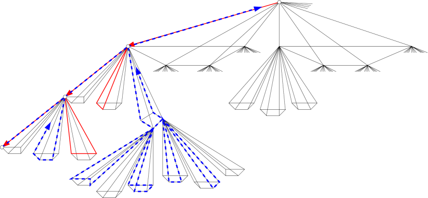
$o=\gamma_{0}$ $\gamma_{1}$ $\gamma_{2}$ $z=\gamma_{3}$ $\Delta_{0,0}$ $\Delta_{0,1}$ $\Delta_{0,2}$

Figure 5.1: A random walk excursion in the pyramid graph $\mathsf{Py}^{3}$ that satisfies the good event $\mathcal{B}_{z}$. The red solid parts are on the way to $z$, the blue dashed ones are on the way back.

Proposition 5.1 (Disconnected nonunimodular $\mathsf{FUSF}$).

For any $d\geq 2$, if $k$ is large enough, and $H$ is a connected finite $d$-regular transitive graph on at least $k^{5/2}$ vertices, then $\mathsf{FUSF}$ on $\mathsf{Py}^{k}\times H$ a.s. has infinitely many components.

Proof. Fix a geodesic ray $\gamma=\gamma(z)=\{o=\gamma_{0},\gamma_{1},\dots,\gamma_{n}=z\}$ from $o$ to $z\in S_{n}$ as before, let $\Delta_{i,0}$ be the pyramid containing both $\gamma_{i}$ and $\gamma_{i+1}$, and let $\Delta_{i,j}$, $j=1,\dots,k-1$, be the other pyramids with their apices at $\gamma_{i}$. Letting $(Y_{t})_{t\geq 0}$ be simple random walk on $\mathsf{Py}^{k}$, started at $o$, the version of the event $\mathcal{B}_{z}$ from (2.2) will be as follows.

$$\begin{aligned} \mathcal{A}_{z}&:=\Big{\{}\textrm{the edge }(\gamma_{i-1},\gamma_{i})\textrm{ is crossed exactly twice by }(Y_{t})_{t=0}^{\tau^{+}_{o}},\\ &\qquad\ \textrm{ and no other edge of }\Delta_{i-1,0}\textrm{ is crossed, for all }i=1,2,\dots,n\Big{\}},\\ \mathcal{L}_{z}&:=\Big{\{}\big{|}\big{\{}t\in\{1,\dots,\tau_{z}\}:Y_{t}=\gamma_{i}\big{\}}\big{|}\leq k/2+1\textrm{, for all }i=1,2,\dots,n\Big{\}}.\end{aligned}$$ (5.1)

Furthermore, let $E_{i}$ and $F_{i}$ be the set of pyramid bases $\Delta_{i,j}\setminus\{\gamma_{i}\}$ visited by $(Y_{t})_{t=0}^{\tau_{z}}$ and by $(Y_{t})_{\tau_{z}}^{\tau^{+}_{o}}$, respectively, among $j=1,\dots,k-1$, and define the event

$$\mathcal{B}_{z}:=\mathcal{A}_{z}\cap\mathcal{L}_{z}\cap\big{\{}E_{i}\cap F_{i}=\emptyset\textrm{ for all }i=1,2,\dots,n\big{\}}.$$ (5.2)

With these definitions, the proofs of Sections 2, 3 go through almost verbatim, with three minor differences. The first one is that all the edges of the pyramids $\Delta_{i,0}$ except for $(\gamma_{i},\gamma_{i+1})$ are forbidden for the random walk, which changes some probabilities by a uniform constant factor, on each level $i$. The second difference is that the graph of pyramids has now the tree structure (and thus, e.g., the self-avoidance condition $E_{i}\cap F_{i}=\emptyset$ is defined via pyramids), but the walk still chooses edges, not pyramids. Again, this can change probabilities only by uniform constant factors. For instance, in place of (2.3) and (2.4), we have

$${{\bf P}\bigl{(}\mathsf{There}_{i},\textrm{ after }j\textrm{ excursions}\bigr{)}}=\left(1-\frac{5}{k}\right)^{j}\frac{1}{4k+1}$$ (5.3)

and

$$p_{k}:={{\bf P}\bigl{(}\mathsf{There}_{i},\ \mathsf{Back}_{i},\textrm{ and }E_{i}\cap F_{i}=\emptyset\bigr{)}}\geq\sum_{j=0}^{\lfloor k/2\rfloor}\left(1-\frac{5}{k}\right)^{j}\frac{1}{4k+1}\frac{1}{4j+2}\asymp\frac{\log k}{k}\,,$$ (5.4)

and everything works just as before.

The last minor difference is in the direct proof of having infinitely many trees almost surely, at the end of Section 3. In the non-unimodular $\mathsf{Py}^{k}$, not all rays $o_{1},o_{2},\dots$ are the same; pick one tending to the distinguished end. Then, it is not obvious that the $\mathsf{Py}^{k}$-coordinate of the simple random walk, viewed only at the times when it moves on this ray, is a one-dimensional symmetric walk. But it is, since the effective conductance between the cutpoints $o_{i}$ and $o_{i+1}$ is obviously equal to the effective conductance between $o_{i}$ and $o_{i-1}$, and hence, by a standard correspondence between hitting probabilities and electric networks [LP16, Chapter 2], we have ${{\bf P}_{o_{i}}(\tau_{o_{i-1}}<\tau_{o_{i+1}})}=1/2$. ∎

Before proving Theorem 1.3, we give our second proof of having infinitely many trees in the $\mathsf{FUSF}$ in the context of tree-like graphs that may also be nonunimodular. The next claim does not include any randomness, and for unimodular transitive graphs it is a tautology.

Proposition 5.2 (Infinite weight sums).

Let $G$ be a transitive graph, $x\in V(G)$ fixed, and $S$ a finite set of vertices such that every component of $G\setminus S$ is infinite. Denote by $\Gamma$ the automorphism group of $G$, and by $\Gamma_{y}$ the stabilizer of a vertex $y$. Then $\sum_{y\in C}\frac{|\Gamma_{y}x|}{|\Gamma_{x}y|}$ is infinite for every component $C$ of $G\setminus S$.

Proof. Let $M>1$ be the maximum of $\frac{|\Gamma_{x}y|}{|\Gamma_{y}x|}$ attained over neighbors $y$ of $x$. For a vertex $v$, let $N_{1}(v)$ be the set of all neighbors $y$ of $v$ with $\frac{|\Gamma_{v}y|}{|\Gamma_{y}v|}=M$. Note that if $y\in N_{1}(v)$ then $\gamma(y)\in N_{1}(\gamma(v))$ for every $\gamma\in\Gamma$. Define recursively $N_{i}(x)=\bigcup_{y\in N_{i-1}(x)}N_{1}(y)$ as $i=2,3,\ldots$. We have $|N_{1}(x)|\geq M$, because $\Gamma_{x}y\subset N_{1}(x)$ and $|\Gamma_{y}x|\geq 1$. We will see next $|N_{i}(x)|\geq M^{i}$.

Choose an arbitrary $y\in N_{i}(x)$. Pick an arbitrary $\gamma\in\Gamma_{x}$, and fix a sequence $x_{j}\in N_{1}(x_{j-1})$ for $j=1,\ldots,i$ with $x_{i}=y$ and $x_{0}:=x$. We will prove by induction that $\gamma(x_{j})\in N_{j}(x)$. For $j=1$ we have seen this. Then, $x_{j}\in N_{1}(x_{j-1})$ implies $\gamma(x_{j})\in N_{1}(\gamma(x_{j-1}))$, and we know $N_{1}(\gamma(x_{j-1}))\subset N_{1}(N_{j-1}(x))=N_{j}(x)$ from the induction hypothesis. This completes the proof of $\Gamma_{x}y\subset N_{i}(x)$. Apply the cocycle identity $\frac{|\Gamma_{u}v|}{|\Gamma_{v}u|}\frac{|\Gamma_{v}w|}{|\Gamma_{w}v|}=\frac{|\Gamma_{u}w|}{|\Gamma_{w}u|}$ to obtain $|N_{i}(x)|\geq|\Gamma_{x}y|={|\Gamma_{y}x|}\frac{|\Gamma_{x_{0}}x_{1}|}{|\Gamma_{x_{1}}x_{0}|}\cdots\frac{|\Gamma_{x_{i-1}}x_{i}|}{|\Gamma_{x_{i}}x_{i-1}|}\geq M^{i}$, as claimed.

For $v\in V(G)$, let $N_{\infty}(v):=\bigcup_{i=1}^{\infty}N_{i}(v)$, and let $m:=\min\Big{\{}\frac{|\Gamma_{s}x|}{|\Gamma_{x}s|}:s\in S\Big{\}}$. If there exists a $v\in C$ such that $\frac{|\Gamma_{v}x|}{|\Gamma_{x}v|}<m$, then $N_{\infty}(v)\cap S=\emptyset$ (using the simple observation that $\frac{|\Gamma_{{v^{\prime}}}x|}{|\Gamma_{x}v^{\prime}|}=\frac{|\Gamma_{v^{\prime}}v|}{|\Gamma_{v}v^{\prime}|}\frac{|\Gamma_{v}x|}{|\Gamma_{x}v|}=M^{-i}\frac{|\Gamma_{v}x|}{|\Gamma_{x}v|}<m$ for every $v^{\prime}\in N_{\infty}(v)$, with some $i\geq 0$), and hence $N_{\infty}(v)\subset C$. Then

$$\sum_{y\in C}\frac{|\Gamma_{y}x|}{|\Gamma_{x}y|}\geq\sum_{y\in N_{\infty}(v)}\frac{|\Gamma_{y}x|}{|\Gamma_{x}y|} =\frac{|\Gamma_{v}x|}{|\Gamma_{x}v|}\sum_{y\in N_{\infty}(v)}\frac{|\Gamma_{y}v|}{|\Gamma_{v}y|}$$

$$=\frac{|\Gamma_{v}x|}{|\Gamma_{x}v|}\sum_{i=1}^{\infty}\sum_{y\in N_{i}(v)}M^{-i}=\frac{|\Gamma_{v}x|}{|\Gamma_{x}v|}\sum_{i=1}^{\infty}|N_{i}(v)|M^{-i}$$

$$\geq\frac{|\Gamma_{v}x|}{|\Gamma_{x}v|}\sum_{i=1}^{\infty}1.$$

If there were no such $v$, then one would have an infinite sum of numbers at least $m$ in $\sum_{y\in C}\frac{|\Gamma_{x}y|}{|\Gamma_{y}x|}$, leading again to the conclusion that the sum is infinite. ∎

Say that $\mathcal{T}$ is a tree-like decomposition of a graph $G$ if $\mathcal{T}$ is a random partition of $V(G)$ into finite connected sets, called bags, together with a tree on the bags such that any edge of $G$ goes between points of adjacent bags or within the same bag. We call a tree-like decomposition invariant if its distribution is preserved by the automorphisms of $G$.

A random spanning forest $\mathcal{F}$ of a graph $G$ was defined to be weak insertion tolerant in [Tim18] if it satisfies the following property. Fix $r>0$ and vertices $x$ and $y$ of $G$ connected by an edge $e$. Let $\mathcal{D}$ be the event that $x$ and $y$ are in different components of $\mathcal{F}$. Then one can map every configuration $\omega\in\mathcal{D}$ to a new configuration $\omega\cup\{e\}\setminus\{f\}$, where $f$ is either the empty set or it is an edge of $\mathcal{F}$ at distance at least $r$ from $x$, and it is determined by $\omega$ in a measurable way. The mapping just defined is measurable, and it takes events of positive probability (contained in $\mathcal{D}$) to events of positive probability (contained in $\mathcal{D}^{c}$). See [Tim18] for a more thorough definition and the proof that the $\mathsf{FUSF}$ and the $\mathsf{FMSF}$ are weak insertion tolerant.

Proposition 5.3 (1 or $\infty$ law).

Let $G$ be an infinite transitive graph that has an invariant random tree-like decomposition. Let $\mathcal{F}$ be an invariant random forest of $G$ with only infinite components, and suppose that it is weak insertion tolerant. Then $\mathcal{F}$ has either 1 or infinitely many components almost surely.

Proof. Proving by contradiction, suppose that $\mathcal{F}$ has $m$ clusters with $1<m<\infty$. Let $\mathcal{T}$ be an invariant random tree-like decomposition of $G$. We claim that with positive probability there exists a bag $B$ and a cluster $\mathcal{C}$ of $\mathcal{F}$ such that $B\cap\mathcal{C}=\emptyset$. To see this, pick a finite $B_{0}\subset G$ such that $B_{0}$ is a bag in $\mathcal{T}$ with positive probability. Condition on this event, and on that some fixed and adjacent $x$ and $y$ in $B_{0}$ are in different $\mathcal{F}$-clusters. (We may assume that $B_{0}$ was chosen so that this event has positive probability.) Let $r>0$ be such that with probability at least $1/2$ any two points of $B_{0}$ that are in the same $\mathcal{F}$-cluster have distance less than $r$ in $\mathcal{F}$. Applying weak insertion tolerance, insert the edge $\{x,y\}$ with the possible removal of an edge at distance at least $r$ from $x$. Repeating this as many times as necessary (at most $|B_{0}|-1$ many times) for some other adjacent pairs in $B_{0}$, we arrive at an event of positive probability where all vertices of $B_{0}$ are in the same $\mathcal{F}$-cluster. But then every other $\mathcal{F}$-cluster has to be fully contained in one of the components of $G\setminus B_{0}$, and hence it cannot intersect the bags in the other components. Thus we have found some $B$ and $\mathcal{C}$ as claimed.

For any $v\in V(G)$, if the bag $B_{v}$ of $v$ does not intersect some $\mathcal{F}$-cluster $\mathcal{C}$, then removing from $\mathcal{T}$ all the bags that intersect $\mathcal{C}$, we get some components, exactly one of which contains $B_{v}$. There is a unique $\mathcal{T}$-edge from a unique bag $B_{v,\mathcal{C}}^{*}$ of this component, to a bag that intersects $\mathcal{C}$. (Possibly $B_{v,\mathcal{C}}^{*}=B_{v}$.) Now, define the following mass transport: for $v,w\in G$,

$$f(v,w,\mathcal{F}):=\sum_{\mathcal{C}}f_{\mathcal{C}}(v,w,\mathcal{F},\mathcal{T}),\qquad f_{\mathcal{C}}(v,w,\mathcal{F},\mathcal{T}):=\begin{cases}{1}/{|B_{v,\mathcal{C}}^{*}|}&\text{if }w\in B_{v,\mathcal{C}}^{*}\text{ for cluster }\mathcal{C}\text{ of }\mathcal{F},\\ 0&\text{otherwise}.\end{cases}$$

We will use the Tilted Mass Transport Principle for invariant percolations on not necessarily unimodular transitive graphs [LP16, Corollary 8.8]: if $\Gamma$ is the automorphism group of $G$, then

$$\sum_{z\in V(G)}\mathbb{E}f(v,z,\mathcal{F},\mathcal{T})=\sum_{y\in V(G)}\mathbb{E}f(y,w,\mathcal{F},\mathcal{T})\,\frac{|\Gamma_{y}w|}{|\Gamma_{w}y|}.$$ (5.5)

The left hand side, which is the expected mass sent out, is clearly at most $m$.

To estimate the right hand side, condition on the event $\mathcal{A}$ that a fixed set $B$ is a bag of $\mathcal{T}$ and it does not intersect some $\mathcal{C}$ but is adjacent to a bag that intersects $\mathcal{C}$. By the first paragraph in the proof, this has a positive probability. Fix a vertex $x$ in $B$. Vertices $y$ in all but one component of $\mathcal{T}\setminus B$ have the property that $B_{y,\mathcal{C}}^{*}=B$, hence they all send mass $1/|B|$ to $x$. Furthermore, every infinite component of $\mathcal{T}\setminus B$ contains an infinite component of $G\setminus B$, hence the right hand side of (5.5) can be bounded from below by $\frac{{\bf P}(\mathcal{A})}{|B|}\mathbb{E}\sum_{y}\frac{|\Gamma_{y}x|}{|\Gamma_{x}y|}$, where $y$ is running over the vertices in some infinite component of $G\setminus B$. (Which infinite component, that may depend on $\mathcal{T}$.) By Proposition 5.2, this sum is always infinite, leading to a contradiction to (5.5). ∎

Once that the $\mathsf{FUSF}$ in $\mathsf{Py}^{k}\times H$ is disconnected with positive probability, Proposition 5.3 gives that it has infinitely many components a.s. by the ergodicity of the $\mathsf{FUSF}$ [LP16, Section 10.4].

Proof of Theorem 1.3. We already know that there are infinitely many trees in the $\mathsf{FUSF}$, and want to show that some of them are light. The fixed end of $\mathsf{Py}^{k}$ yields a natural projection $\pi:\mathsf{Py}^{k}\times H\relbar\joinrel\twoheadrightarrow\mathbb{Z}$, where all the preimages $x\in\pi^{-1}(m)$ for a fixed $m\in\mathbb{Z}$ have the same Haar weight $\mu(\Gamma_{x})=(4k)^{-m}$.

If all the infinitely many clusters $\mathcal{C}_{i}$ in the $\mathsf{FUSF}$ were reaching infinitely high up in Figure 5.1, i.e., if $\inf\pi(\mathcal{C}_{i})=-\infty$, then, for any two $\mathcal{C}_{i},\mathcal{C}_{j}$ there would exist some $\gamma_{m(i,j)}\in\pi^{-1}(m(i,j))$ such that the infinite geodesic ray $\gamma_{m(i,j)},\gamma_{m(i,j)-1},\dots$ in $\mathsf{Py}^{k}$, converging to the fixed end at $-\infty$, has the property that both clusters intersect each $\gamma_{m(i,j)-t}\times H$, for $t=0,1,\dots$. However, if we take enough clusters $\{\mathcal{C}_{i}\}_{i\in I}$ such that ${|I|\choose 2}>|H|$, and let $m:=\min\{m(i,j):i,j\in I\}$, then $\gamma_{m}$ is already defined for each pair, and it is actually the same vertex of $\mathsf{Py}^{k}$, so we would need to have ${|I|\choose 2}$ disjoint clusters intersecting $\gamma_{m}\times H$, a contradiction.

Thus, all but finitely many clusters $\mathcal{C}_{i}$ of $\mathsf{FUSF}$ have a smallest label $\min\pi(\mathcal{C}_{i})>-\infty$. Let $M(\mathcal{C}_{i})\subset G$ be the set of vertices achieving this minimal label; we set $M(\mathcal{C}_{i})=\emptyset$ if $\inf\pi(\mathcal{C}_{i})=-\infty$. Note that $|M(\mathcal{C}_{i})|\leq H$ almost surely. Now, define the following mass transport: for $x,y\in G$,

$$f(x,y,\mathsf{FUSF}):=\begin{cases}1&\text{if }x,y\text{ are in the same component }\mathcal{C}_{i}\text{ of }\mathsf{FUSF},\text{ and }y\in M(\mathcal{C}_{i}),\\ 0&\text{otherwise}.\end{cases}$$

We again use the Tilted Mass Transport Principle from [LP16, Corollary 8.8]:

$$\sum_{y\in V(G)}\mathbb{E}f(x,y,\mathsf{FUSF})=\sum_{y\in V(G)}\mathbb{E}f(y,x,\mathsf{FUSF})\,\frac{\mu(\Gamma_{y})}{\mu(\Gamma_{x})}.$$ (5.6)

The left hand side is at most $|H|$. The right hand side, if $x\in M(\mathcal{C}_{i})$ for some cluster $\mathcal{C}_{i}$, is

$$(4k)^{\min\pi(\mathcal{C}_{i})}\sum_{y\in\mathcal{C}_{i}}\mu(\Gamma_{y}).$$

By (5.6), this is finite, hence, whenever $\min\pi(\mathcal{C}_{i})>-\infty$, the cluster $\mathcal{C}_{i}$ is light.∎

6 Tell me why

The first natural question is how general the phenomena of Theorems 1.1 and 1.2 really are:

Problem 6.1.

If $\Gamma$ is a finitely generated treeable group with $\mathsf{WUSF}\not=\mathsf{FUSF}$, does it always have two generating sets such that the $\mathsf{FUSF}$ is disconnected in the first Cayley graph, while it is connected in the second?

Tom Hutchcroft has suggested that $\mathbb{Z}^{5}*\mathbb{Z}^{5}$ might be a counterexample, where the disconnectedness of the $\mathsf{FUSF}$ cannot be destroyed. However, a proof does not seem to be a trivial matter to us.

An affirmative answer for the connected case would of course imply $\beta^{(2)}_{1}(\Gamma)=\mathsf{cost}(\Gamma)-1$ for treeable groups, which is actually known to hold by Gaboriau’s results [Gab02, Corollaries 3.23 and 3.16].

For our specific Cayley graphs of Theorem 1.1, the following two problems remain open. Of course, a negative answer to Problem 6.2 would be pointing towards a positive answer to Problem 6.3.

Problem 6.2.

Is it true that if the $\mathsf{FUSF}$ in some $\mathbb{T}^{k}\times H$ is disconnected, then any two components touch each other only at finitely many places? Are there at least special choices for $k$ and $H$ for which this happens?

Problem 6.3.

For the $\mathsf{FUSF}$ in any $\mathbb{T}^{k}\times H$, is the union of the $\mathsf{FUSF}$ with an independent $\mathsf{Bernoulli}(\epsilon)$ bond percolation connected, for any $\epsilon>0$? If not, is there any invariant way to make the $\mathsf{FUSF}$ connected by adding an arbitrarily small density edge percolation?

As we already defined in the introduction, for any finite graph $H$ we let

$$\mathsf{disco}(H):=\min\big{\{}k:\mathsf{FUSF}(\mathbb{T}^{k}\times H)\textrm{ is disconnected}\big{\}}\in\{3,4,\dots,\infty\}.$$

We know that $\mathsf{disco}(P_{2})=\infty$ from [Tan19], while Theorem 1.1 implies that if $\ell$ is large enough, then the cycle $C_{\ell}$ of length $\ell$ has $\mathsf{disco}(C_{\ell})<\infty$.

Problem 6.4.

What is the smallest $\ell$ for which $\mathsf{disco}(C_{\ell})<\infty$? In particular, what is $\mathsf{disco}(C_{3})$?

Problem 6.5.

Are there infinitely many finite graphs $H$ with $\mathsf{disco}(H)=\infty$?

The two choices for $H$ in Theorem 1.2 inspire the following question:

Problem 6.6.

If $H$ and $H^{\prime}$ are two finite connected graphs on the same vertex set and $E(H)\subset E(H^{\prime})$, do we always have $\mathsf{disco}(H)\leq\mathsf{disco}(H^{\prime})$?

Far from this monotonicity, but a similar type of result was shown in [ABIT20+]: for any $\mathbb{T}^{k}\times H$, if we increase the weights on the edges of $H$ enough, then the $\mathsf{FUSF}$ becomes connected.

Regarding the generality of Lemma 4.1, we have not found the following question addressed in the literature. One piece of motivation is [PR04].

Problem 6.7.

Is it true on any connected transitive graph on $n$ vertices that the typical size of the stationary loop-erased version of a simple random walk trajectory is $\Omega(\sqrt{n})$?

Now, given how the proof of Theorem 1.1 used Lemma 3.2, and how the proof of Theorem 1.2 used Lemma 4.1, one may guess that if $H$ has better mixing properties, then disconnection becomes easier:

Problem 6.8.

If $H$ and $H^{\prime}$ are two connected transitive $d$-regular finite graphs on the same vertex set, with $H^{\prime}$ having a spectral gap larger than $H$, does it follow that $\mathsf{disco}(H)\geq\mathsf{disco}(H^{\prime})$?

The next natural player appearing on the floor is $\mathsf{disco}^{*}$, a parameter that is dual, in some sense, to $\mathsf{disco}$. Let us fix a natural sequence of finite graphs $\mathcal{H}=(H_{n})_{n\geq 1}$; as the simplest case, think of the cycles $H_{n}=C_{n}$. Then let

$$\mathsf{disco}^{*}_{\mathcal{H}}(k):=\min\big{\{}n:\mathsf{FUSF}(\mathbb{T}^{k}\times H_{n})\textrm{ is disconnected}\big{\}}.$$

Problem 6.9.

Consider the sequence of cycles $\mathcal{C}=(C_{n})_{n\geq 1}$. Is it the case that $\mathsf{disco}^{*}_{\mathcal{C}}(3)<\infty$?

Problem 6.10.

How about monotonicity in $k$? That is, if $\mathsf{FUSF}(\mathbb{T}^{k}\times H)$ is disconnected, then is $\mathsf{FUSF}(\mathbb{T}^{k+1}\times H)$ also disconnected?

One can also define a continuous version of the graph parameter $\mathsf{disco}$. Recall from [AL07] or [Pet20, Chapter 14] what unimodular random rooted graphs are.

$$\widetilde{\mathsf{disco}}(H):=\inf \big{\{}\kappa:\mathsf{FUSF}(\mathcal{T}\times H)\textrm{ is disconnected with positive probability},$$

$$(\mathcal{T},o)\textrm{ is an infinite unimodular random rooted tree with }\mathbb{E}\deg_{\mathcal{T}}(o)=\kappa\big{\}}\in[2,\infty].$$

Problem 6.11.

Find $\widetilde{\mathsf{disco}}(C_{\ell})$.

Problem 6.12.

Is there any finite graph $H$ with $\widetilde{\mathsf{disco}}(H)<\infty=\mathsf{disco}(H)$?

Problem 6.13.

Is there any finite graph $H$ with $\widetilde{\mathsf{disco}}(H)=2$? (Note that if $\mathbb{E}\deg_{\mathcal{T}}(o)=2$, then $\mathcal{T}$ has at most two ends, hence $\mathcal{T}\times H$ is recurrent, hence the $\mathsf{FUSF}$ is connected almost surely. However, this does not exclude the possibility of the infimum being 2.) Or perhaps $\widetilde{\mathsf{disco}}(H)<\infty$ implies $\widetilde{\mathsf{disco}}(H)=2$?

Tributes

We are indebted to Russ Lyons and Pengfei Tang for comments and corrections on the manuscript. We also thank Tom Hutchcroft and Péter Mester for useful remarks, and Damien Gaboriau and Asaf Nachmias for some references. Our work was supported by the ERC Consolidator Grant 772466 “NOISE”. The second author was partially supported by Icelandic Research Fund Grant 185233-051.

Gábor Pete
Alfréd Rényi Institute of Mathematics, Budapest,
and Institute of Mathematics, Budapest University of Technology and Economics
http://www.math.bme.hu/~gabor
gabor.pete [at] renyi.hu

Ádám Timár
Division of Mathematics, The Science Institute, University of Iceland
and Alfréd Rényi Institute of Mathematics
madaramit [at] gmail.com

References

- [AL07] D. Aldous and R. Lyons. Processes on unimodular random networks. Electron. J. Probab. 12 (2007), Paper 54, 1454–1508. http://mypage.iu.edu/~rdlyons/#urn
- [ABIT20+] M. Alexy, M. Borbényi, A. Imolay, and Á. Timár. Connectedness of the Free Uniform Spanning Forest as a function of edge weights. arXiv:2011.12904 [math.PR]
- [AHNR18] O. Angel, T. Hutchcroft, A. Nachmias, and G. Ray. Hyperbolic and parabolic unimodular random maps. Geometric and Functional Analysis 28 (2018), 879–942. arXiv:1612.08693 [math.PR]
- [BV97] B. Bekka and A. Valette. Group cohomology, harmonic functions and the first -Betti number. Potential Analysis 6 (1997), 313–326. https://link.springer.com/article/10.1023/A:1017974406074
- [Ben91] I. Benjamini. Instability of the Liouville property for quasi-isometric graphs and manifolds of polynomial volume growth. J. Theor. Probab., 4 (1991), 632–636. https://link.springer.com/content/pdf/10.1007/BF01210328.pdf
- [BKPS04] I. Benjamini, H. Kesten, Y. Peres and O. Schramm. Geometry of the uniform spanning forest: transitions in dimensions 4, 8, 12, …. Ann. of Math. (2) 160 (2004), 465–491. [arXiv:math.PR/0107140]
- [BLPS01] I. Benjamini, R. Lyons, Y. Peres and O. Schramm. Uniform spanning forests. Ann. Probab. 29 (2001), 1–65. https://www.jstor.org/stable/2652913
- [DLP12] J. Ding, J. Lee, and Y. Peres. Cover times, blanket times, and majorizing measures. Ann. Math. 175 (2012), 1409–1471. arXiv:1004.4371 [math.PR]
- [Dur10] R. Durrett. Probability: Theory and Examples. Fourth edition. Cambridge University Press, 2010. https://services.math.duke.edu/~rtd/PTE/pte.html
- [Dyn84] E. B. Dynkin. Gaussian and non-Gaussian random fields associated with Markov processes. J. Funct. Anal. 55 (1984), 344–376. https://www.sciencedirect.com/science/article/pii/0022123684900041
- [Gab02] D. Gaboriau. Invariants de relations d’équivalence et de groupes. Publ. Math. Inst. Hautes Études Sci. 95 (2002), 93–150. http://www.numdam.org/article/PMIHES_2002__95__93_0.pdf
- [Hut18] T. Hutchcroft. Interlacements and the Wired Uniform Spanning Forest. Ann. Probab. 46 (2018), 1170–1200. arXiv:1512.08509 [math.PR]
- [HN17] T. Hutchcroft and A. Nachmias. Indistinguishability of trees in uniform spanning forests. Probab. Theory Related Fields 168 (2017), 113–152. arXiv:1506.00556 [math.PR]
- [HN19] T. Hutchcroft and A. Nachmias. Uniform spanning forests of planar graphs. Forum of Mathematics, Sigma 7 (2019), e29, pp. 55. arXiv:1603.07320 [math.PR]
- [HP20] T. Hutchcroft and G. Pete. Kazhdan groups have cost 1. Inv. Math. (2020), to appear. arXiv:1810.11015 [math.GR]
- [LPW17] D. A. Levin, Y. Peres and E. L. Wilmer. Markov chains and mixing times. Second edition. With a chapter by J. G. Propp and D. B. Wilson. American Mathematical Society, Providence, RI, 2017. http://pages.uoregon.edu/dlevin/MARKOV/
- [Lup16] T. Lupu. From loop clusters and random interlacement to the free field. Ann. Probab. 44 (2016), 2117–2146. arXiv:1402.0298 [math.PR]
- [Lyo05] R. Lyons. Asymptotic enumeration of spanning trees. Combin. Probab. & Comput. 14 (2005), 491–522. [arXiv:math.CO/0212165]
- [LP16] R. Lyons and Y. Peres. Probability on Trees and Networks. Cambridge University Press, New York, 2016. Available at http://pages.iu.edu/~rdlyons/
- [LPS06] R. Lyons, Y. Peres and O. Schramm. Minimal spanning forests. Ann. Probab. 34 (2006), 1665–1692. [arXiv:math.PR/0412263]
- [Mor03] B. Morris. The components of the wired spanning forest are recurrent. Probab. Theory Related Fields 125 (2003), 259–265. https://link.springer.com/article/10.1007/s00440-002-0236-0
- [MP05] B. Morris and Y. Peres. Evolving sets, mixing and heat kernel bounds. Probab. Theory Related Fields 133 (2005), 245–266. [arXiv:math.PR/0305349]
- [PSN00] I. Pak and T. Smirnova-Nagnibeda. On non-uniqueness of percolation on nonamenable Cayley graphs. Compt. Rendus Acad. Sci. Math. 330 (2000), No. 6, 495–500. http://www.math.ucla.edu/~pak/papers/psn.pdf
- [PP00] R. Pemantle and Y. Peres. Nonamenable products are not treeable. Israel J. Math. 118 (2000), 147–155. [arXiv:math.PR/0404096]
- [PR04] Y. Peres and D. Revelle. Scaling limits of the uniform spanning tree and loop-erased random walk on finite graphs. [arXiv:math/0410430]
- [Pet20] G. Pete. Probability and Geometry on Groups. Book in preparation, http://www.math.bme.hu/~gabor/PGG.pdf
- [Soa93] P. M. Soardi. Rough isometries and Dirichlet finite harmonic functions on graphs. Proc. Amer. Math. Soc. 119 (1993), 1239–1248. https://www.jstor.org/stable/2159987
- [Tan19] P. Tang. Weights of uniform spanning forests on nonunimodular transitive graphs. arXiv:1908.09889 [math.PR]
- [Tho15] A. Thom. A remark about the spectral radius. Intern. Math. Res. Notices 10 (2015), 2856–2864. arXiv:1306.1767 [math.GR]
- [Tim06] Á. Timár. Neighboring clusters in Bernoulli percolation. Ann. Probab. 34 (2006), 2332–2343. [arXiv:math.PR/0702873]
- [Tim18] Á. Timár. Indistinguishability of the components of random spanning forests. Ann. Probab. 46 (2018), 2221–2242. arXiv:1506.01370 [math.PR]
- [Tim19+] Á. Timár. Unimodular random planar graphs are sofic. arXiv:1910.01307 [math.PR]
- [Zha18] A. Zhai. Exponential concentration of cover times. Electron. J. Probab. 23 (2018), no. 32, 1–22. arXiv:1407.7617 [math.PR]
- [Wil96] D. B. Wilson. Generating random spanning trees more quickly than the cover time. Proceedings of the Twenty-Eighth Annual ACM Symposium on the Theory of Computing, pp. 296–303., New York, 1996. https://dl.acm.org/doi/pdf/10.1145/237814.237880