Pointer Graph Networks

Abstract

Graph neural networks (GNNs) are typically applied to static graphs that are assumed to be known upfront. This static input structure is often informed purely by insight of the machine learning practitioner, and might not be optimal for the actual task the GNN is solving. In absence of reliable domain expertise, one might resort to inferring the latent graph structure, which is often difficult due to the vast search space of possible graphs. Here we introduce Pointer Graph Networks (PGNs) which augment sets or graphs with additional inferred edges for improved model generalisation ability. PGNs allow each node to dynamically point to another node, followed by message passing over these pointers. The sparsity of this adaptable graph structure makes learning tractable while still being sufficiently expressive to simulate complex algorithms. Critically, the pointing mechanism is directly supervised to model long-term sequences of operations on classical data structures, incorporating useful structural inductive biases from theoretical computer science. Qualitatively, we demonstrate that PGNs can learn parallelisable variants of pointer-based data structures, namely disjoint set unions and link/cut trees. PGNs generalise out-of-distribution to $5\times$ larger test inputs on dynamic graph connectivity tasks, outperforming unrestricted GNNs and Deep Sets.

1 Introduction

Graph neural networks (GNNs) have seen recent successes in applications such as quantum chemistry [14], social networks [32] and physics simulations [1, 23, 34]. For problems where a graph structure is known (or can be approximated), GNNs thrive. This places a burden upon the practitioner: which graph structure should be used? In many applications, particularly with few nodes, fully connected graphs work well, but on larger problems, sparsely connected graphs are required. As the complexity of the task imposed on the GNN increases and, separately, the number of nodes increases, not allowing the choice of graph structure to be data-driven limits the applicability of GNNs.

Classical algorithms [5] span computations that can be substantially more expressive than typical machine learning subroutines (e.g. matrix multiplications), making them hard to learn, and a good benchmark for GNNs [4, 8]. Prior work has explored learning primitive algorithms (e.g. arithmetic) by RNNs [57, 20, 45], neural approximations to NP-hard problems [50, 25], making GNNs learn (and transfer between) graph algorithms [47, 13], recently recovering a single neural core [55] capable of sorting, path-finding and binary addition. Here, we propose Pointer Graph Networks (PGNs), a framework that further expands the space of general-purpose algorithms that can be neurally executed.

Idealistically, one might imagine the graph structure underlying GNNs should be fully learnt from data, but the number of possible graphs grows super-exponentially in the number of nodes [39], making searching over this space a challenging (and interesting) problem. In addition, applying GNNs further necessitates the learning of the messages passed on top of the learnt structure, making it hard to disambiguate errors from having either the wrong structure or the wrong message. Several approaches have been proposed for searching over the graph structure [27, 16, 23, 21, 52, 9, 36, 19, 28]. Our PGNs take a hybrid approach, assuming that the practitioner may specify part of the graph structure, and then adaptively learn a linear number of pointer edges between nodes (as in [50] for RNNs). The pointers are optimised through direct supervision on classical data structures [5]. We empirically demonstrate that PGNs further increase GNN generalisation beyond those with static graph structures [12], without sacrificing computational cost or sparsity for this added flexibility in graph structure.

Unlike prior work on algorithm learning with GNNs [54, 47, 55, 6, 40], we consider algorithms that do not directly align to dynamic programming (making them inherently non-local [53]) and, crucially, the optimal known algorithms rely upon pointer-based data structures. The pointer connectivity of these structures dynamically changes as the algorithm executes. We learn algorithms that operate on two distinct data structures—disjoint set unions [11] and link/cut trees [38]. We show that baseline GNNs are unable to learn the complicated, data-driven manipulations that they perform and, through PGNs, show that extending GNNs with learnable dynamic pointer links enables such modelling.

Finally, the hallmark of having learnt an algorithm well, and the purpose of an algorithm in general, is that it may be applied to a wide range of input sizes. Thus by learning these algorithms we are able to demonstrate generalisation far beyond the size of training instance included in the training set.

Our PGN work presents three main contributions: we expand neural algorithm execution [54, 47, 55] to handle algorithms relying on complicated data structures; we provide a novel supervised method for sparse and efficient latent graph inference; and we demonstrate that our PGN model can deviate from the structure it is imitating, to produce useful and parallelisable data structures.

2 Problem setup and PGN architecture

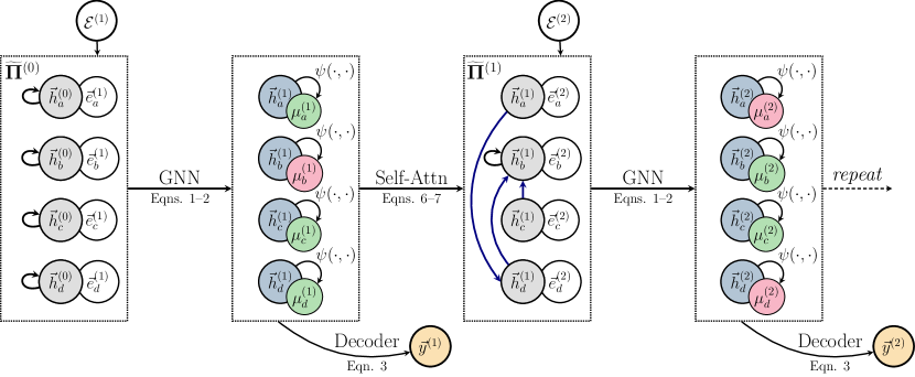
Figure 1: High-level overview of the pointer graph network (PGN) dataflow. Using descriptions of entity operations ($\vec{e}_{i}^{(t)}$), the PGN re-estimates latent features $\vec{h}_{i}^{(t)}$, masks $\mu_{i}^{(t)}$, and (asymmetric) pointers $\widetilde{\mathbf{\Pi}}^{(t)}$. The symmetrised pointers, ${\mathbf{\Pi}}^{(t)}$, are then used as edges for a GNN that computes next-step latents, $\vec{h}_{i}^{(t+1)}$, continuing the process. The latents may be used to provide answers, $\vec{y}^{(t)}$, to queries about the underlying data. We highlight masked out nodes in red, and modified pointers and latents in blue. See Appendix A for a higher-level visualisation, along with PGN’s gradient flow.

Problem setup

We consider the following sequential supervised learning setting: Assume an underlying set of $n$ entities. Given are sequences of inputs $\mathcal{E}^{(1)},\mathcal{E}^{(2)},\ldots$ where $\mathcal{E}^{(t)}=(\vec{e}_{1}^{(t)},\vec{e}_{2}^{(t)},\dots,\vec{e}_{n}^{(t)})$ for $t\geq 1$ is defined by a list of feature vectors $\vec{e}^{(t)}_{i}\in\mathbb{R}^{m}$ for every entity $i\in\{1,\ldots,n\}$. We will suggestively refer to $\vec{e}^{(t)}_{i}$ as an operation on entity $i$ at time $t$. The task consists now in predicting target outputs $\vec{y}^{(t)}\in\mathbb{R}^{l}$ based on operation sequence $\mathcal{E}^{(1)},\ldots,\mathcal{E}^{(t)}$ up to $t$.

A canonical example for this setting is characterising graphs with dynamic connectivity, where inputs $\vec{e}_{i}^{(t)}$ indicate edges being added/removed at time $t$, and target outputs $\vec{y}^{(t)}$ are binary indicators of whether pairs of vertices are connected. We describe this problem in-depth in Section 3.

Pointer Graph Networks

As the above sequential prediction task is defined on the underlying, un-ordered set of entities, any generalising prediction model is required to be invariant under permutations of the entity set [49, 30, 56]. Furthermore, successfully predicting target $\vec{y}^{(t)}$ in general requires the prediction model to maintain a robust data structure to represent the history of operations for all entities throughout their lifetime. In the following we present our proposed prediction model, the Pointer Graph Network (PGN), that combines these desiderata in an efficient way.

At each step $t$, our PGN model computes latent features $\vec{h}_{i}^{(t)}\in\mathbb{R}^{k}$ for each entity $i$. Initially, $\vec{h}_{i}^{(0)}=\vec{0}$. Further, the PGN model determines dynamic pointers—one per entity and time step—which may be summarised in a pointer adjacency matrix ${\mathbf{\Pi}}^{(t)}\in\mathbb{R}^{n\times n}$. Pointers correspond to undirected edges between two entities: indicating that one of them points to the other. ${\mathbf{\Pi}}^{(t)}$ is a binary symmetric matrix, indicating locations of pointers as 1-entries. Initially, we assume each node points to itself: ${\mathbf{\Pi}}^{(0)}={\bf I}_{n}$. A summary of the coming discussion may be found in Figure 1.

The Pointer Graph Network follows closely the encode-process-decode [17] paradigm. The current operation is encoded together with the latents in each entity using an encoder network $f$:

$$\vec{z}_{i}^{(t)}=f\left(\vec{e}_{i}^{(t)},\vec{h}_{i}^{(t-1)}\right)$$ (1)

after which the derived entity representations ${\bf Z}^{(t)}=(\vec{z}_{1}^{(t)},\vec{z}_{2}^{(t)},\dots,\vec{z}_{n}^{(t)})$ are given to a processor network, $P$, which takes into account the current pointer adjacency matrix as relational information:

$${\bf H}^{(t)}=P\left({\bf Z}^{(t)},{\mathbf{\Pi}}^{(t-1)}\right)$$ (2)

yielding next-step latent features, ${\bf H}^{(t)}=(\vec{h}_{1}^{(t)},\vec{h}_{2}^{(t)},\dots,\vec{h}_{n}^{(t)})$; we discuss choices of $P$ below. These latents can be used to answer set-level queries using a decoder network $g$:

$$\vec{y}^{(t)}=g\left(\bigoplus_{i}\vec{z}_{i}^{(t)},\bigoplus_{i}\vec{h}_{i}^{(t)}\right)$$ (3)

where $\bigoplus$ is any permutation-invariant readout aggregator, such as summation or maximisation.

Many efficient data structures only modify a small subset of the entities at once [5]. We can incorporate this inductive bias into PGNs by masking their pointer modifications through a sparse mask $\mu_{i}^{(t)}\in\{0,1\}$ for each node that is generated by a masking network $\psi$:

$$\mathbb{P}\left(\mu_{i}^{(t)}=1\right)=\psi\left(\vec{z}_{i}^{(t)},\vec{h}_{i}^{(t)}\right)$$ (4)

where the output activation function for $\psi$ is the logistic sigmoid function, enforcing the probabilistic interpretation. In practice, we threshold the output of $\psi$ as follows:

$$\mu_{i}^{(t)}=\mathbb{I}_{\psi\left(\vec{z}_{i}^{(t)},\vec{h}_{i}^{(t)}\right)>0.5}$$ (5)

The PGN now re-estimates the pointer adjacency matrix ${\mathbf{\Pi}}^{(t)}$ using $\vec{h}_{i}^{(t)}$. To do this, we leverage self-attention [46], computing all-pairs dot products between queries $\vec{q}_{i}^{(t)}$ and keys $\vec{k}_{i}^{(t)}$:

$$\vec{q}_{i}^{(t)}={\bf W}_{q}\vec{h}_{i}^{(t)}\qquad\vec{k}_{i}^{(t)}={\bf W}_{k}\vec{h}_{i}^{(t)}\qquad\alpha_{ij}^{(t)}=\mathrm{softmax}_{j}\left(\left<\vec{q}_{i}^{(t)},\vec{k}_{j}^{(t)}\right>\right)$$ (6)

where ${\bf W}_{q}$ and ${\bf W}_{k}$ are learnable linear transformations, and $\left<\cdot,\cdot\right>$ is the dot product operator. $\alpha_{ij}^{(t)}$ indicates the relevance of entity $j$ to entity $i$, and we derive the pointer for $i$ by choosing entity $j$ with the maximal $\alpha_{ij}$. To simplify the dataflow, we found it beneficial to symmetrise this matrix:

$$\widetilde{\mathbf{\Pi}}_{ij}^{(t)}=\mu_{i}^{(t)}\widetilde{\mathbf{\Pi}}_{ij}^{(t-1)}+\left(1-\mu_{i}^{(t)}\right)\mathbb{I}_{j=\mathrm{argmax}_{k}\left(\alpha_{ik}^{(t)}\right)}\qquad{\mathbf{\Pi}}_{ij}^{(t)}=\widetilde{\mathbf{\Pi}}_{ij}^{(t)}\vee\widetilde{\mathbf{\Pi}}_{ji}^{(t)}$$ (7)

where $\mathbb{I}$ is the indicator function, $\widetilde{\mathbf{\Pi}}^{(t)}$ denotes the pointers before symmetrisation, $\lor$ denotes logical disjunction between the two operands, and $1-{\mu}_{i}^{(t)}$ corresponds to negating the mask. Nodes $i$ and $j$ will be linked together in ${\mathbf{\Pi}}^{(t)}$ (i.e., ${\mathbf{\Pi}}_{ij}^{(t)}=1$) if $j$ is the most relevant to $i$, or vice-versa.

Unlike prior work which relied on the Gumbel trick [21, 23], we will provide direct supervision with respect to ground-truth pointers, $\hat{\mathbf{\Pi}}^{(t)}$, of a target data structure. Applying $\mu_{i}^{(t)}$ effectively masks out parts of the computation graph for Equation 6, yielding a graph attention network-style update [48].

Further, our data-driven conditional masking is reminiscent of neural execution engines (NEEs) [55]. Therein, masks were used to decide which inputs are participating in the computation at any step; here, instead, masks are used to determine which output state to overwrite, with all nodes participating in the computations at all times. This makes our model’s hidden state end-to-end differentiable through all steps (see Appendix A), which was not the case for NEEs.

While Equation 6 involves computation of $O(n^{2})$ coefficients, this constraint exists only at training time; at test time, computing entries of ${\mathbf{\Pi}}^{(t)}$ reduces to 1-NN queries in key/query space, which can be implemented storage-efficiently [31]. The attention mechanism may also be sparsified, as in [24].

PGN components and optimisation

In our implementation, the encoder, decoder, masking and key/query networks are all linear layers of appropriate dimensionality—placing most of the computational burden on the processor, $P$, which explicitly leverages the computed pointer information.

In practice, $P$ is realised as a graph neural network (GNN), operating over the edges specified by $\mathbf{\Pi}^{(t-1)}$. If an additional input graph between entities is provided upfront, then its edges may be also included, or even serve as a completely separate “head” of GNN computation.

Echoing the results of prior work on algorithmic modelling with GNNs [47], we recovered strongest performance when using message passing neural networks (MPNNs) [14] for $P$, with elementwise maximisation aggregator. Hence, the computation of Equation 2 is realised as follows:

$$\vec{h}_{i}^{(t)}=U\left(\vec{z}_{i}^{(t)},\max_{{\mathbf{\Pi}}^{(t-1)}_{ji}=1}M\left(\vec{z}_{i}^{(t)},\vec{z}_{j}^{(t)}\right)\right)$$ (8)

where $M$ and $U$ are linear layers producing vector messages. Accordingly, we found that elementwise-max was the best readout operation for $\bigoplus$ in Equation 3; while other aggregators (e.g. sum) performed comparably, maximisation had the least variance in the final result. This is in line with its alignment to the algorithmic task, as previously studied [33, 54]. We apply ReLU to the outputs of $M$ and $U$.

Besides the downstream query loss in $\vec{y}^{(t)}$ (Equation 3), PGNs optimise two additional losses, using ground-truth information from the data structure they are imitating: cross-entropy of the attentional coefficients $\alpha_{ij}^{(t)}$ (Equation 6) against the ground-truth pointers, $\hat{\mathbf{\Pi}}^{(t)}$, and binary cross-entropy of the masking network $\psi$ (Equation 4) against the ground-truth entities being modified at time $t$. This provides a mechanism for introducing domain knowledge in the learning process. At training time we readily apply teacher forcing, feeding ground-truth pointers and masks as input whenever appropriate. We allow gradients to flow from these auxiliary losses back in time through the latent states $\vec{h}_{i}^{(t)}$ and $\vec{z}_{i}^{(t)}$ (see Appendix A for a diagram of the backward pass of our model).

PGNs share similarities with and build on prior work on using latent $k$-NN graphs [9, 21, 52], primarily through addition of pointer-based losses against a ground-truth data structure and explicit entity masking—which will prove critical to generalising out-of-distribution in our experiments.

3 Task: Dynamic graph connectivity

We focus on instances of the dynamic graph connectivity setup to illustrate the benefits of PGNs. Even the simplest of structural detection tasks are known to be very challenging for GNNs [4], motivating dynamic connectivity as one example of a task where GNNs are unlikely to perform optimally.

Dynamic connectivity querying is an important subroutine in computer science, e.g. when computing minimum spanning trees—deciding if an edge can be included in the solution without inducing cycles [26], or maximum flow—detecting existence of paths from source to sink with available capacity [7].

Formally, we consider undirected and unweighted graphs of $n$ nodes, with evolving edge sets through time; we denote the graph at time $t$ by $G^{(t)}=(V,E^{(t)})$. Initially, we assume the graphs to be completely disconnected: $E^{(0)}=\emptyset$. At each step, an edge $(u,v)$ may be added to or removed from $E^{(t-1)}$, yielding $E^{(t)}=E^{(t-1)}\ominus\{(u,v)\}$, where $\ominus$ is the symmetric difference operator.

A connectivity query is then defined as follows: for a given pair of vertices $(u,v)$, does there exist a path between them in $G^{(t)}$? This yields binary ground-truth query answers $\hat{y}^{(t)}$ which we can supervise towards. Several classical data structures exist for answering variants of connectivity queries on dynamic graphs, on-line, in sub-linear time [11, 37, 38, 44] of which we will discuss two. All the derived inputs and outputs to be used for training PGNs are summarised in Appendix B.

Incremental graph connectivity with disjoint-set unions

We initially consider incremental graph connectivity: edges can only be added to the graph. Knowing that edges can never get removed, it is sufficient to combine connected components through set union. Therefore, this problem only requires maintaining disjoint sets, supporting an efficient union(u, v) operation that performs a union of the sets containing $u$ and $v$. Querying connectivity then simply requires checking whether $u$ and $v$ are in the same set, requiring an efficient find(u) operation which will retrieve the set containing $u$.

To put emphasis on the data structure modelling, we consider a combined operation on $(u,v)$: first, query whether $u$ and $v$ are connected, then perform a union on them if they are not. Pseudocode for this query-union(u, v) operation is given in Figure 2 (Right). query-union is a key component of important algorithms, such as Kruskal’s algorithm [26] for minimum spanning trees.—which was not modellable by prior work [47].

$\proc{Init}(u)$ $\hat{\pi}_{u}\leftarrow u$ $r_{u}\sim\mathcal{U}(0,1)$ $\proc{Find}(u)$ $\hat{\pi}_{u}\neq u$ $\hat{\pi}_{u}$

$\proc{Union}(u,v)$ $x\leftarrow\proc{Find}(u)$ $y\leftarrow\proc{Find}(v)$ $x\neq y$ $r_{x}<r_{y}$ $\hat{\pi}_{x}\leftarrow y$ $\hat{\pi}_{y}\leftarrow x$

$\proc{Query-Union}(u,v)$ $\proc{Find}(u)=\proc{Find}(v)$ $0$ $\hat{y}^{(t)}=0$ $\proc{Union}(u,v)$ $1$ $\hat{y}^{(t)}=1$

Figure 2: Pseudocode of DSU operations; initialisation and find(u) (Left), union(u, v) (Middle) and query-union(u, v), giving ground-truth values of $\hat{y}^{(t)}$ (Right). All manipulations of ground-truth pointers $\hat{\mathbf{\Pi}}$ ($\hat{\pi}_{u}$ for node $u$) are in blue; the path compression heuristic is highlighted in green.

The tree-based disjoint-set union (DSU) data structure [11] is known to yield optimal complexity [10] for this task. DSU represents sets as rooted trees—each node, $u$, has a parent pointer, $\hat{\pi}_{u}$—and the set identifier will be its root node, $\rho_{u}$, which by convention points to itself ($\hat{\pi}_{\rho_{u}}=\rho_{u}$). Hence, find(u) reduces to recursively calling find(pi[u]) until the root is reached—see Figure 2 (Left). Further, path compression [41] is applied: upon calling find(u), all nodes on the path from $u$ to $\rho_{u}$ will point to $\rho_{u}$. This self-organisation substantially reduces future querying time along the path.

Calling union(u, v) reduces to finding the roots of $u$ and $v$’s sets, then making one of these roots point to the other. To avoid pointer ambiguity, we assign a random priority, $r_{u}\sim\mathcal{U}(0,1)$, to every node at initialisation time, then always preferring the node with higher priority as the new root—see Figure 2 (Middle). This approach of randomised linking-by-index [15] was recently shown to achieve time complexity of $O(\alpha(n))$ per operation in expectancy, which is optimal.

Casting to the framework of Section 2: at each step $t$, we call query-union(u, v), specified by operation descriptions $\vec{e}_{i}^{(t)}=r_{i}\|\mathbb{I}_{i=u\vee i=v}$, containing the nodes’ priorities, along with a binary feature indicating which nodes are $u$ and $v$. The corresponding output $\hat{y}^{(t)}$ indicates the return value of the query-union(u, v). Finally, we provide supervision for the PGN’s (asymmetric) pointers, $\widetilde{\mathbf{\Pi}}^{(t)}$, by making them match the ground-truth DSU’s pointers, $\hat{\pi}_{i}$ (i.e., $\hat{\mathbf{\Pi}}^{(t)}_{ij}=1$ iff $\hat{\pi}_{i}=j$ and $\hat{\mathbf{\Pi}}^{(t)}_{ij}=0$ otherwise.). Ground-truth mask values, $\hat{\mu}_{i}^{(t)}$, are set to $0$ for only the paths from $u$ and $v$ to their respective roots—no other node’s state is changed (i.e., $\hat{\mu}_{i}^{(t)}=1$ for the remaining nodes).

Before moving on, consider how having access to these pointers helps the PGN answer queries, compared to a baseline without them: checking connectivity of $u$ and $v$ boils down to following their pointer links and checking if they meet, which drastically relieves learning pressure on its latent state.

Fully dynamic tree connectivity with link/cut trees

We move on to fully dynamic connectivity—edges may now be removed, and hence set unions are insufficient to model all possible connected component configurations. The problem of fully dynamic tree connectivity—with the restriction that $E^{(t)}$ is acyclic—is solvable in amortised $O(\log n)$ time by link/cut trees (LCTs) [38], elegant data structures that maintain forests of rooted trees, requiring only one pointer per node.

The operations supported by LCTs are: find-root(u) retrieves the root of node $u$; link(u, v) links nodes $u$ and $v$, with the precondition that $u$ is the root of its own tree; cut(v) removes the edge from $v$ to its parent; evert(u) re-roots $u$’s tree, such that $u$ becomes the new root.

LCTs also support efficient path-aggregate queries on the (unique) path from $u$ to $v$, which is very useful for reasoning on dynamic trees. Originally, this speeded up bottleneck computations in network flow algorithms [7]. Nowadays, the LCT has found usage across online versions of many classical graph algorithms, such as minimum spanning forests and shortest paths [42]. Here, however, we focus only on checking connectivity of $u$ and $v$; hence find-root(u) will be sufficient for our queries.

Similarly to our DSU analysis, here we will compress updates and queries into one operation, query-toggle(u, v), which our models will attempt to support. This operation first calls evert(u), then checks if $u$ and $v$ are connected: if they are not, adding the edge between them wouldn’t introduce cycles (and $u$ is now the root of its tree), so link(u, v) is performed. Otherwise, cut(v) is performed—it is guaranteed to succeed, as $v$ is not going to be the root node. Pseudocode of query-toggle(u, v), along with visualising the effects of running it, is provided in Figure 3.

We encode each query-toggle(u, v) as $\vec{e}_{i}^{(t)}=r_{i}\|\mathbb{I}_{i=u\vee i=v}$. Random priorities, $r_{i}$, are again used; this time to determine whether $u$ or $v$ will be the node to call evert on, breaking ambiguity. As for DSU, we supervise the asymmetric pointers, $\widetilde{\mathbf{\Pi}}^{(t)}$, using the ground-truth LCT’s pointers, $\hat{\pi}_{i}$ and ground-truth mask values, $\hat{\mu}_{i}^{(t)}$, are set to $0$ only if $\hat{\pi}_{i}$ is modified in the operation at time $t$. Link/cut trees require elaborate bookkeeping; for brevity, we delegate further descriptions of their operations to Appendix C, and provide our C++ implementation of the LCT in the supplementary material.

$\proc{Query-Toggle}(u,v)$ $r_{u}<r_{v}$ $\proc{Swap}(u,v)$ $\proc{Evert}(u)$ $\proc{Find-Root}(v)\neq u$ $\proc{Link}(u,v)$ 0 $\hat{y}^{(t)}=0$ $\proc{Cut}(v)$ 1 $\hat{y}^{(t)}=1$

 

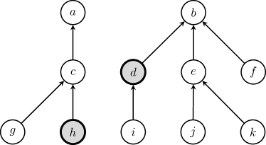
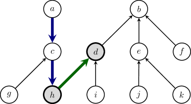
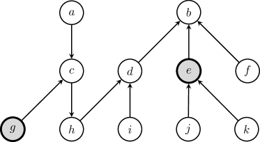
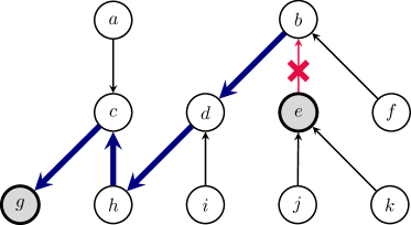
Figure 3: Left: Pseudocode of the query-toggle(u, v) operation, which will be handled by our models; Right: Effect of calling query-toggle(h, d) on a specific forest (Top), followed by calling query-toggle(g, e) (Bottom). Edges affected by evert (blue), link (green), and cut (red) are highlighted. N.B. this figure represents changes to the forest being modelled, and not the underlying LCT pointers; see Appendix C for more information on pointer manipulation.

4 Evaluation and results

Experimental setup

As in [47, 55], we evaluate out-of-distribution generalisation—training on operation sequences for small input sets ($n=20$ entities with $\mathrm{ops}=30$ operations), then testing on up to $5\times$ larger inputs ($n=50,\mathrm{ops}=75$ and $n=100,\mathrm{ops}=150$). In line with [47], we generate 70 sequences for training, and 35 sequences across each test size category for testing. We generate operations $\vec{e}_{i}^{(t)}$ by sampling input node pairs $(u,v)$ uniformly at random at each step $t$; query-union(u, v) or query-toggle(u, v) is then called to generate ground-truths $\hat{y}^{(t)}$, $\hat{\mu}_{i}^{(t)}$ and $\hat{\mathbf{\Pi}}^{(t)}$. This is known to be a good test-bed for spanning many possible DSU/LCT configurations and benchmarking various data structures (see e.g. Section 3.5 in [42]).

All models compute $k=32$ latent features in each layer, and are trained for $5,000$ epochs using Adam [22] with learning rate of $0.005$. We perform early stopping, retrieving the model which achieved the best query F₁ score on a validation set of 35 small sequences ($n=20,\mathrm{ops}=30$). We attempted running the processor (Equation 8) for more than one layer between steps, and using a separate GNN for computing pointers—neither yielding significant improvements.

We evaluate the PGN model of Section 2 against three baseline variants, seeking to illustrate the benefits of its various graph inference components. We describe the baselines in turn.

Deep Sets [56] independently process individual entities, followed by an aggregation layer for resolving queries. This yields an only-self-pointer mechanism, ${\mathbf{\Pi}}^{(t)}={\bf I}_{n}$ for all $t$, within our framework. Deep Sets are popular for set-based summary statistic tasks. Only the query loss is used.

(Unrestricted) GNNs [14, 35, 54] make no prior assumptions on node connectivity, yielding an all-ones adjacency matrix: ${\mathbf{\Pi}}^{(t)}_{ij}=1$ for all $(t,i,j)$. Such models are a popular choice when relational structure is assumed but not known. Only the query loss is used.

PGN without masks (PGN-NM) remove the masking mechanism of Equations 4–7. This repeatedly overwrites all pointers, i.e. $\mu_{i}^{(t)}=0$ for all $(i,t)$. PGN-NM is related to a directly-supervised variant of the prior art in learnable $k$-NN graphs [9, 21, 52]. PGN-NM has no masking loss in its training.

These models are universal approximators on permutation-invariant inputs [54, 56], meaning they are all able to model the DSU and LCT setup perfectly. However, unrestricted GNNs suffer from oversmoothing as graphs grow [58, 3, 51, 29], making it harder to perform robust credit assignment of relevant neighbours. Conversely, Deep Sets must process the entire operation history within their latent state, in a manner that is decomposable after the readout—which is known to be hard [54].

To assess the utility of the data structure learnt by the PGN mechanism, as well as its performance limits, we perform two tests with fixed pointers, supervised only on the query:

PGN-Ptrs: first, a PGN model is learnt on the training data. Then it is applied to derive and fix the pointers ${\mathbf{\Pi}}^{(t)}$ at all steps for all training/validation/test inputs. In the second phase, a new GNN over these inferred pointers is learnt and evaluated, solely on query answering.

Oracle-Ptrs: learn a query-answering GNN over the ground-truth pointers $\hat{\mathbf{\Pi}}^{(t)}$. Note that this setup is, especially for link/cut trees, made substantially easier than PGN: the model no longer needs to imitate the complex sequences of pointer rotations of LCTs.

Results and discussion

Our results, summarised in Table 1, clearly indicate outperformance and generalisation of our PGN model, especially on the larger-scale test sets. Competitive performance of PGN-Ptrs implies that the PGN models a robust data structure that GNNs can readily reuse. While the PGN-NM model is potent in-distribution, its performance rapidly decays once it is tasked to model larger sets of pointers at test time. Further, on the LCT task, baseline models often failed to make very meaningful advances at all—PGNs are capable of surpassing this limitation, with a result that even approaches ground-truth pointers with increasing input sizes.

We corroborate some of these results by evaluating pointer accuracy (w.r.t. ground truth) with the analysis in Table 2. Without masking, the PGNs fail to meaningfully model useful pointers on larger test sets, whereas the masked PGN consistently models the ground-truth to at least $50\%$ accuracy. Mask accuracies remain consistently high, implying that the inductive bias is well-respected.

Table 1: F₁ scores on the dynamic graph connectivity tasks for all models considered, on five random seeds. All models are trained on $n=20,\textrm{ops}=30$ and tested on larger test sets.

Model	Disjoint-set union			Link/cut tree
	$n=20$	$n=50$	$n=100$	$n=20$	$n=50$	$n=100$
	$\mathrm{ops}=30$	$\mathrm{ops}=75$	$\mathrm{ops}=150$	$\mathrm{ops}=30$	$\mathrm{ops}=75$	$\mathrm{ops}=150$
GNN	$0.892{\scriptscriptstyle\pm.007}$	$0.851{\scriptscriptstyle\pm.048}$	$0.733{\scriptscriptstyle\pm.114}$	$0.558{\scriptscriptstyle\pm.044}$	$0.510{\scriptscriptstyle\pm.079}$	$0.401{\scriptscriptstyle\pm.123}$
Deep Sets	$0.870{\scriptscriptstyle\pm.029}$	$0.720{\scriptscriptstyle\pm.132}$	$0.547{\scriptscriptstyle\pm.217}$	$0.515{\scriptscriptstyle\pm.080}$	$0.488{\scriptscriptstyle\pm.074}$	$0.441{\scriptscriptstyle\pm.068}$
PGN-NM	${\bf 0.910}{\scriptscriptstyle\pm.011}$	$0.628{\scriptscriptstyle\pm.071}$	$0.499{\scriptscriptstyle\pm.096}$	$0.524{\scriptscriptstyle\pm.063}$	$0.367{\scriptscriptstyle\pm.018}$	$0.353{\scriptscriptstyle\pm.029}$
PGN	$0.895{\scriptscriptstyle\pm.006}$	${\bf 0.887}{\scriptscriptstyle\pm.008}$	${\bf 0.866}{\scriptscriptstyle\pm.011}$	${\bf 0.651}{\scriptscriptstyle\pm.017}$	${\bf 0.624}{\scriptscriptstyle\pm.016}$	${\bf 0.616}{\scriptscriptstyle\pm.009}$
PGN-Ptrs	$0.902{\scriptscriptstyle\pm.010}$	$0.902{\scriptscriptstyle\pm.008}$	$0.889{\scriptscriptstyle\pm.007}$	$0.630{\scriptscriptstyle\pm.022}$	$0.603{\scriptscriptstyle\pm.036}$	$0.546{\scriptscriptstyle\pm.110}$
Oracle-Ptrs	$0.944{\scriptscriptstyle\pm.006}$	$0.964{\scriptscriptstyle\pm.007}$	$0.968{\scriptscriptstyle\pm.013}$	$0.776{\scriptscriptstyle\pm.011}$	$0.744{\scriptscriptstyle\pm.026}$	$0.636{\scriptscriptstyle\pm.065}$

Table 2: Pointer and mask accuracies of the PGN model w.r.t. ground-truth pointers.

Accuracy of	Disjoint-set union			Link/cut tree
	$n=20$	$n=50$	$n=100$	$n=20$	$n=50$	$n=100$
	$\mathrm{ops}=30$	$\mathrm{ops}=75$	$\mathrm{ops}=150$	$\mathrm{ops}=30$	$\mathrm{ops}=75$	$\mathrm{ops}=150$
Pointers (NM)	${\bf 80.3}{\scriptscriptstyle\pm 2.2\%}$	$32.9{\scriptscriptstyle\pm 2.7\%}$	$20.3{\scriptscriptstyle\pm 3.7\%}$	${\bf 61.3}{\scriptscriptstyle\pm 5.1\%}$	$17.8{\scriptscriptstyle\pm 3.3\%}$	$8.4{\scriptscriptstyle\pm 2.1\%}$
Pointers	$76.9{\scriptscriptstyle\pm 3.3\%}$	${\bf 64.7}{\scriptscriptstyle\pm 6.6\%}$	${\bf 55.0}{\scriptscriptstyle\pm 4.8\%}$	$60.0{\scriptscriptstyle\pm 1.3\%}$	${\bf 54.7}{\scriptscriptstyle\pm 1.9\%}$	${\bf 53.2}{\scriptscriptstyle\pm 2.2\%}$
Masks	$95.0{\scriptscriptstyle\pm 0.9\%}$	$96.4{\scriptscriptstyle\pm 0.6\%}$	$97.3{\scriptscriptstyle\pm 0.4\%}$	$82.8{\scriptscriptstyle\pm 0.9\%}$	$86.8{\scriptscriptstyle\pm 1.1\%}$	$91.1{\scriptscriptstyle\pm 1.0\%}$

Using the max readout in Equation 3 provides an opportunity for a qualitative analysis of the PGN’s credit assignment. DSU and LCT focus on paths from the two nodes operated upon to their roots in the data structure, implying they are highly relevant to queries. As each global embedding dimension is pooled from exactly one node, in Appendix D we visualise how often these relevant nodes appear in the final embedding—revealing that the PGN’s inductive bias amplifies their credit substantially.

Rollout analysis of PGN pointers

Figure 4: Visualisation of a PGN rollout on the DSU setup, for a pathological ground-truth case of repeated union(i, i+1) (Left). The first few pointers in ${\mathbf{\Pi}}^{(t)}$ are visualised (Middle) as well as the final state (Right)—the PGN produced a valid DSU at all times, but $2\times$ shallower than ground-truth.

Tables 1–2 indicate a substantial deviation of PGNs from the ground-truth pointers, $\hat{\mathbf{\Pi}}^{(t)}$, while maintaining strong query performance. These learnt pointers are still meaningful: given our 1-NN-like inductive bias, even minor discrepancies that result in modelling invalid data structures can have negative effects on the performance, if done uninformedly.

We observe the learnt PGN pointers on a pathological DSU example (Figure 4). Repeatedly calling query-union(i, i+1) with nodes ordered by priority yields a linearised DSU. Such graphs (of large diameter) are difficult for message propagation with GNNs. During rollout, the PGN models a correct DSU at all times, but halving its depth—easing GNN usage and GPU parallelisability.

Effectively, the PGN learns to use the query supervision from $y^{(t)}$ to “nudge” its pointers in a direction more amenable to GNNs, discovering parallelisable data structures which may substantially deviate from the ground-truth $\hat{\mathbf{\Pi}}^{(t)}$. Note that this also explains the reduced performance gap of PGNs to Oracle-Ptrs on LCT; as LCTs cannot apply path-compression-like tricks, the ground-truth LCT pointer graphs are expected to be of substantially larger diameters as test set size increases.

Ablation studies

In Table 3, we provide results of several additional models, designed to probe additional hypotheses about the PGNs’ contribution. These models are as follows:

• The contribution of our PGN model is two-fold: introducing inductive biases (such as pointers and masking) and usage of additional supervision (such as intermediate data structure rollouts). To verify that our gains do not arise from supervision alone, we evaluate SupGNN, the GNN model which features masking and pointer losses, but doesn’t actually use this information. The model outperforms the GNN, while still being significantly behind our PGN results—implying our empirical gains are due to inductive biases as well.

• Our model’s direct usage of data structure hints allows it to reason over highly relevant links. To illustrate the benefits of doing so, we also attempt training the pointers using the differentiable graph module (DGM) [21] loss function. DGM treats the model’s downstream performance as a reward function for the chosen pointers. This allows it to outperform the baseline models, but not as substantially as PGN.

• Conversely from our SupGNN experiment, our inductive biases can be strong enough to allow useful behaviour to emerge even in limited supervision scenarios. We were interested in how well the PGN would perform if we only had a sense of which data needs to be changed at each iteration—i.e. supervising on masks only (PGN-MO) and letting the pointers adjust to nearest-neighbours (as done in [52]) without additional guidance. On average, our model outperforms all non-PGN models—demonstrating that even knowing only the mask information can be sufficient for PGNs to achieve state-of-the-art performance on out-of-distribution reasoning tasks.

• Our PGN model uses the symmetrised pointers ${\mathbf{\Pi}}$, where $i$ pointing to $j$ implies we will add both edges $i\rightarrow j$ and $j\rightarrow i$ for the GNN to use. This does not strictly align with the data structure, but we assumed that, empirically, it will allow the model to make mistakes more “gracefully”, without disconnecting critical components of the graph. To this end, we provide results for PGN-Asym, where the pointer matrix remains asymmetric. We recover results that are significantly weaker than the PGN result, but still outperforming all other baselines on average. While this result demonstrates the empirical value of our approach to rectifying mistakes in the pointer mechanism, we acknowledge that better approaches are likely to exist—and we leave their study to future work.

Results are provided on the hardest LCT test set ($n=100,\mathrm{ops}=150$); the results on the remaining test sets mirror these findings. We note that multiple GNN steps may be theoretically required to reconcile our work with teacher forcing the data structure. We found it sufficient to consider one-step in all of our experiments, but as tasks get more complex—especially when compression is no longer applicable—dynamic number of steps (e.g. function of dataset size) is likely to be appropriate.

Lastly, we scaled up the LCT test set to ($n=200,\mathrm{ops}=300$) where the PGN ($0.636{\scriptstyle\pm.009}$) catches up to Oracle-Ptr ($0.619{\scriptstyle\pm.043}$). This illustrates not only the robustness of PGNs to larger test sets, but also provides a quantitative substantiation to our claim about ground-truth LCTs not having favourable diameters.

Table 3: $\mathrm{F}_{1}$ scores on the largest link/cut tree test set ($n=100,\mathrm{ops}=150$) for four ablated models; the results on other datasets mirror these findings. GNN and PGN results reproduced from Table 1.

GNN	SupGNN	DGM	PGN-MO	PGN-Asym	PGN
$0.401{\scriptstyle\pm.123}$	$0.541{\scriptstyle\pm.059}$	$0.524{\scriptstyle\pm.104}$	$0.558{\scriptstyle\pm.022}$	$0.561{\scriptstyle\pm.035}$	${\bf 0.616}{\scriptstyle\pm.009}$

5 Conclusions

We presented pointer graph networks (PGNs), a method for simultaneously learning a latent pointer-based graph and using it to answer challenging algorithmic queries. Introducing step-wise structural supervision from classical data structures, we incorporated useful inductive biases from theoretical computer science, enabling outperformance of standard set-/graph-based models on two dynamic graph connectivity tasks, known to be challenging for GNNs. Out-of-distribution generalisation, as well as interpretable and parallelisable data structures, have been recovered by PGNs.

Broader Impact

Our work evaluates the extent to which existing neural networks are potent reasoning systems, and the minimal ways (e.g. inductive biases / training regimes) to strengthen their reasoning capability. Hence our aim is not to outperform classical algorithms, but make their concepts accessible to neural networks. PGNs enable reasoning over edges not provided in the input, simplifying execution of any algorithm requiring a pointer-based data structure. PGNs can find direct practical usage if, e.g., they are pre-trained on known algorithms and then deployed on tasks which may require similar kinds of reasoning (with encoders/decoders “casting” the new problem into the PGN’s latent space).

It is our opinion that this work does not have a specific immediate and predictable real-world application and hence no specific ethical risks associated. However, PGN offers a natural way to introduce domain knowledge (borrowed from data structures) into the learning of graph neural networks, which has the potential of improving their performance, particularly when dealing with large graphs. Graph neural networks have seen a lot of successes in modelling diverse real world problems, such as social networks, quantum chemistry, computational biomedicine, physics simulations and fake news detection. Therefore, indirectly, through improving GNNs, our work could impact these domains and carry over any ethical risks present within those works.

Appendix A Pointer graph networks gradient computation

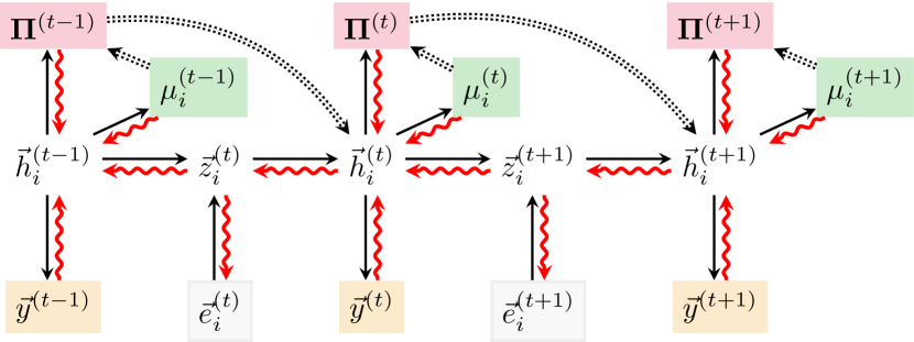
Figure 5: Detailed view of the dataflow within the PGN model, highlighting inputs $\vec{e}_{i}^{(t)}$ (outlined), objects optimised against ground-truths (query answers $\vec{y}^{(t)}$, masks $\mu_{i}^{(t)}$ and pointers ${\mathbf{\Pi}}^{(t)}$) (shaded) and all intermediate latent states ($\vec{z}_{i}^{(t)}$ and $\vec{h}_{i}^{(t)}$). Solid lines indicate differentiable computation with gradient flow in red, while dotted lines indicate non-differentiable opeations (teacher-forced at training time). N.B. This computation graph should also include edges from $\vec{z}_{i}^{(t)}$ into the query answers, masks and pointers (as it gets concatenated with $\vec{h}_{i}^{(t)}$)—we omit these edges for clarity.

To provide a more high-level overview of the PGN model’s dataflow across all relevant variables (and for realising its computational graph and differentiability), we provide the visualisation in Figure 5.

Most operations of the PGN are realised as standard neural network layers and are hence differentiable; the two exceptions are the thresholding operations that decide the final masks $\mu_{i}^{(t)}$ and pointers ${\mathbf{\Pi}}^{(t)}$, based on the soft coefficients computed by the masking network and the self-attention, respectively. This makes no difference to the training algorithm, as the masks and pointers are teacher-forced, and the soft coefficients are directly optimised against ground-truth values of $\hat{\mu}_{i}^{(t)}$ and $\hat{\mathbf{\Pi}}^{(t)}$.

Further, note that our setup allows a clear path to end-to-end backpropagation (through the latent vectors) at all steps, allowing the representation of $\vec{h}_{i}^{(t)}$ to be optimised with respect to all predictions made for steps $t^{\prime}>t$ in the future.

Appendix B Summary of operation descriptions and supervision signals

Table 4: Summary of operation descriptions and supervision signals on the data structures considered.

Data structure	Operation descriptions, $\vec{e}_{i}^{(t)}$	Supervision signals
and operation
Disjoint-set union [11] query-union(u, v)	$r_{i}$: randomly sampled priority of node $i$, $\mathbb{I}_{i=u\vee i=v}$: Is node $i$ being operated on?	$\hat{y}^{(t)}$: are $u$ and $v$ in the same set?,
		$\hat{\mu}_{i}^{(t)}$: is node $i$ visited by find(u)
		or find(v)?,
		$\hat{\mathbf{\Pi}}_{ij}^{(t)}$: is $\hat{\pi}_{i}=j$ after executing?
		(asymmetric pointer)
Link/cut tree [38] query-toggle(u, v)	$r_{i}$: randomly sampled priority of node $i$, $\mathbb{I}_{i=u\vee i=v}$: Is node $i$ being operated on?	$\hat{y}^{(t)}$: are $u$ and $v$ connected?,
		$\hat{\mu}_{i}^{(t)}$: is node $i$ visited during
		query-toggle(u, v)?,
		$\hat{\mathbf{\Pi}}_{ij}^{(t)}$: is $\hat{\pi}_{i}=j$ after executing?
		(asymmetric pointer)

To aid clarity, within Table LABEL:tab:summary, we provide an overview of all the operation descriptions and outputs (supervision signals) for the data structures considered here (disjoint-set unions and link/cut trees).

Note that the manipulation of ground-truth pointers ($\hat{\pi}_{i}$) is not discussed for LCTs in the main text for purposes of brevity; for more details, consult Appendix C.

Appendix C Link/cut tree operations

In this section, we provide a detailed overview of the link/cut tree (LCT) data structure [38], as well as the various operations it supports. This appendix is designed to be as self-contained as possible, and we provide the C++ implementation used to generate our dataset within the supplementary material.

Before covering the specifics of LCT operations, it is important to understand how it represents the forest it models; namely, in order to support efficient $O(\log n)$ operations and path queries, the pointers used by the LCT can differ significantly from the edges in the forest being modelled.

Preferred path decomposition

Many design choices in LCTs follow the principle of “most-recent access”: if a node was recently accessed, it is likely to get accessed again soon—hence we should keep it in a location that makes it easily accessible.

The first such design is preferred path decomposition: the modelled forest is partitioned into preferred paths, such that each node may have at most one preferred child: the child most-recently accessed during a node-to-root operation. As we will see soon, any LCT operation on a node $u$ will involve looking up the path to its respective root $\rho_{u}$—hence every LCT operation will be be composed of several node-to-root operations.

One example of a preferred path decomposition is demonstrated in Figure 6 (Left). Note how each node may have at most one preferred child. When a node is not a preferred child, its parent edge is used to jump between paths, and is hence often called a path-parent.

LCT pointers

Each preferred path is represented by LCTs in a way that enables fast access—in a binary search tree (BST) keyed by depth. This implies that the nodes along the path will be stored in a binary tree (each node will potentially have a left and/or right child) which respects the following recursive invariant: for each node, all nodes in its left subtree will be closer to the root, and all nodes in its right subtree will be further from the root.

For now, it is sufficient to recall the invariant above—the specific implementation of binary search trees used in LCTs will be discussed towards the end of this section. It should be apparent that these trees should be balanced: for each node, its left and right subtree should be of (roughly) comparable sizes, recovering an optimal lookup complexity of $O(\log n)$, for a BST of $n$ nodes.

Each of the preferred-path BSTs will specify its own set of pointers. Additionally, we still need to include the path-parents, to allow recombining information across different preferred paths. While we could keep these links unchanged, it is in fact canonical to place the path-parent in the root node of the path’s BST (N.B. this node may be different from the top-of-path node!).

As we will notice, this will enable more elegant operation of the LCT, and further ensures that each LCT node will have exactly one parent pointer (either in-BST parent or path-parent, allowing for jumping between different path BSTs), which aligns perfectly with our PGN model assumptions.

The ground-truth pointers of LCTs, $\hat{\mathbf{\Pi}}^{(t)}$, are then recovered as all the parent pointers contained within these binary search trees, along with all the path-parents. Similarly, ground-truth masks, $\hat{\mu}_{i}^{(t)}$, will be the subset of LCT nodes whose pointers may change during the operation at time $t$. We illustrate how a preferred path decomposition can be represented with LCTs within Figure 6 (Right).

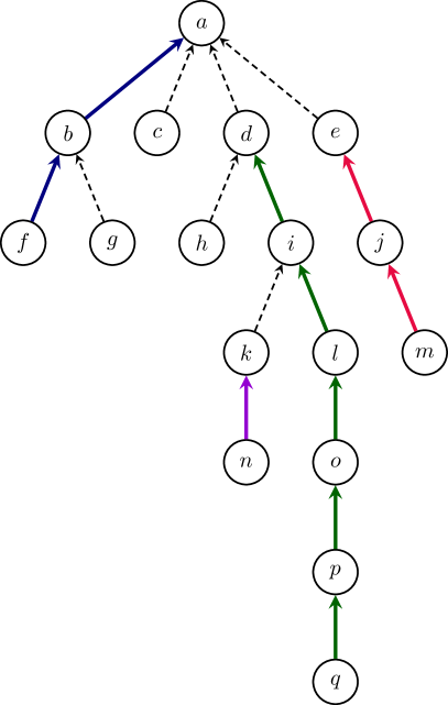
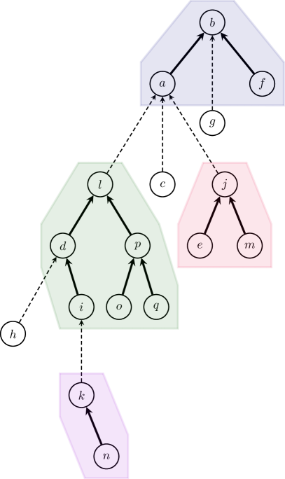
Figure 6: Left: Rooted tree modelled by LCTs, with its four preferred paths indicated by solid lines. The most-recently accessed path is $f\rightarrow b\rightarrow a$. Right: One possible configuration of LCT pointers which models the tree. Each preferred path is stored in a binary search tree (BST) keyed by depth (colour-coded to match the LHS figure), and path-parents (dashed) emanate from the root node of each BST—hence their source node may changed (e.g. $d\twoheadrightarrow a$ is represented as $l\twoheadrightarrow a$).

LCT operations

Now we are ready to cover the specifics of how individual LCT operations (find-root(u), link(u, v), cut(u) and evert(u)) are implemented.

All of these operations rely on an efficient operation which exposes the path from a node $u$ to its root, making it preferred—and making $u$ the root of the entire LCT (i.e. the root node of the top-most BST). We will denote this operation as expose(u), and assume its implementation is provided to us for now. As we will see, all of the interesting LCT operations will necessarily start with calls to expose(u) for nodes we are targeting.

Before discussing each of the LCT operations, note one important invariant after running expose(u): node $u$ is now the root node of the top-most BST (containing the nodes on the path from $u$ to $\rho_{u}$), and it has no right children in this BST—as it is the deepest node in this path.

As in the main document, we will highlight in blue all changes to the ground-truth LCT pointers $\hat{\pi}_{u}$, which will be considered as the union of ground-truth BST parents $\hat{p}_{u}$ and path-parents $\hat{pp}_{u}$. Note that each node $u$ will either have $\hat{p}_{u}$ or $\hat{pp}_{u}$; we will denote unused pointers with nil. By convention, root nodes, $\rho$, of the entire LCT will point to themselves using a BST parent; i.e. $\hat{p}_{\rho}=\rho$, $\hat{pp}_{\rho}=\textsc{nil}$.

• find-root(u) can be implemented as follows: first execute expose(u). This guarantees that $u$ is in the same BST as $\rho_{u}$, the root of the entire tree. Now, since the BST is keyed by depth and $\rho_{u}$ is the shallowest node in the BST’s preferred path, we just follow left children while possible, starting from $u$: $\rho_{u}$ is the node at which this is no longer possible. We conclude with calling expose on $\rho_{u}$, to avoid pathological behaviour of repeatedly querying the root, accumulating excess complexity from following left children. $\proc{Find-Root}(u)$ $\proc{Expose}(u)$ $\rho_{u}\leftarrow u$ $\mathrm{left}_{\rho_{u}}\neq\const{nil}$ While currently considered node has left child $\rho_{u}\leftarrow\mathrm{left}_{\rho_{u}}$ Follow left child links $\proc{Expose}(\rho_{u})$ Re-expose to avoid pathological complexity $\rho_{u}$

• link(u, v) has the precondition that $u$ must be the root node of its respective tree (i.e. $u=\rho_{u}$), and $u$ and $v$ are not in the same tree. We start by running expose(u) and expose(v). Attaching the edge $u\rightarrow v$ extends the preferred path from $v$ to its root, $\rho_{v}$, to incorporate $u$. Given that $u$ can have no left children in its BST (it is a root node, hence shallowest), this can be done simply by making $v$ a left child of $u$ (given $v$ is shallower than $u$ on the path $u\rightarrow v\rightarrow\dots\rightarrow\rho_{v}$). $\proc{Link}(u,v)$ $\proc{Expose}(u)$ $\proc{Expose}(v)$ $\mathrm{left}_{u}\leftarrow v$ $u$ cannot have left-children before this, as it is the root of its tree $\hat{p}_{v}\leftarrow u$ $v$ cannot have parents before this, as it has been exposed

• cut(u), as above, will initially execute expose(u). As a result, $u$ will retain all the nodes that are deeper than it (through path-parents pointed to by $u$), and can just be cut off from all shallower nodes along the preferred path (contained in $u$’s left subtree, if it exists). $\proc{Cut}(u)$ $\proc{Expose}(u)$ $\mathrm{left}_{u}\neq\const{nil}$ $\hat{p}_{\mathrm{left}_{u}}\leftarrow\mathrm{left}_{u}$ Cut off $u$ from left child, making it a root node of its component $\mathrm{left}_{u}\leftarrow\const{nil}$

• evert(u), as visualised in Figure 3, needs to isolate the path from $u$ to $\rho_{u}$, and flip the direction of all edges along it. The first part is already handled by calling expose(u), while the second is implemented by recursively flipping left and right subtrees within the entire BST containing $u$ (this makes shallower nodes in the path become deeper, and vice-versa).

  This is implemented via lazy propagation: each node $u$ stores a flip bit, $\phi_{u}$ (initially set to 0). Calling evert(u) will toggle node $u$’s flip bit. Whenever we process node $u$, we further issue a call to a special operation, release(u), which will perform any necessary flips of $u$’s left and right children, followed by propagating the flip bit onwards. Note that release(u) does not affect parent-pointers $\hat{\pi}_{u}$—but it may affect outcomes of future operations on them. $\proc{Release}(u)$ $u\neq\const{nil}$ and $\phi_{u}=1$ $\proc{Swap}(\mathrm{left}_{u},\mathrm{right}_{u})$ Perform the swap of $u$’s left and right subtrees $\mathrm{left}_{u}\neq\const{nil}$ $\phi_{\mathrm{left}_{u}}\leftarrow\phi_{\mathrm{left}_{u}}\oplus 1$ Propagate flip bit to left subtree $\mathrm{right}_{u}\neq\const{nil}$ $\phi_{\mathrm{right}_{u}}\leftarrow\phi_{\mathrm{right}_{u}}\oplus 1$ Propagate flip bit to right subtree $\phi_{u}=0$ $\proc{Evert}(u)$ $\proc{Expose}(u)$ $\phi_{u}\leftarrow\phi_{u}\oplus 1$ Toggle $u$’s flip bit ($\oplus$ is binary exclusive OR) $\proc{Release}(u)$ Perform lazy propagation of flip bit from $u$

Implementing expose(u)

It only remains to provide an implementation for expose(u), in order to specify the LCT operations fully.

LCTs use splay trees as the particular binary search tree implementation to represent each preferred path. These trees are also designed with “most-recent access” in mind: nodes recently accessed in a splay tree are likely to get accessed again, therefore any accessed node is turned into the root node of the splay tree, using the splay(u) operation. The manner in which splay(u) realises its effect is, in turn, via a sequence of complex tree rotations; such that rotate(u) will perform a rotation that brings $u$ one level higher in the tree.

We describe these three operations in a bottom-up fashion: first, the lowest-level rotate(u), which merely requires carefully updating all the pointer information. Depending on whether $u$ is its parent’s left or right child, a zig or zag rotation is performed—they are entirely symmetrical. Refer to Figure 7 for an example of a zig rotation followed by a zag rotation (often called zig-zag for short).

$\proc{Rotate}(u)$ $v\leftarrow\hat{p}_{u}$ $w\leftarrow\hat{p}_{v}$ $\mathrm{left}_{v}=u$ Zig rotation $\mathrm{left}_{v}\leftarrow\mathrm{right}_{u}$ $\mathrm{right}_{u}\neq\const{nil}$ $\hat{p}_{\mathrm{right}_{u}}\leftarrow v$ $\mathrm{right}_{u}\leftarrow v$ Zag rotation $\mathrm{right}_{v}\leftarrow\mathrm{left}_{u}$ $\mathrm{left}_{u}\neq\const{nil}$ $\hat{p}_{\mathrm{left}_{u}}\leftarrow v$ $\mathrm{left}_{u}\leftarrow v$ $\hat{pp}_{u}\leftarrow\hat{pp}_{v}$ $\hat{p}_{v}\leftarrow u$ $\hat{pp}_{v}\leftarrow\const{nil}$ $w\neq\const{nil}$ Adjust grandparent $\mathrm{left}_{w}=v$ $\mathrm{left}_{w}=u$ $\mathrm{right}_{w}=u$ $\hat{p}_{u}\leftarrow w$

Figure 7: A schematic of a zig-zag rotation: first, node $u$ is rotated around node $v$; then, node $u$ is rotated around node $w$, bringing it two levels higher in the BST without breaking invariants.

Armed with the rotation primitive, we may define splay(u) as a repeated application of zig, zig-zig and zig-zag rotations, until node $u$ becomes the root of its BST. We also repeatedly perform lazy propagation by calling release(u) on any encountered nodes.

$\proc{Splay}(u)$ $\hat{p}_{u}\neq\const{nil}$ Repeat while $u$ is not BST root $v\leftarrow\hat{p}_{u}$ $w\leftarrow\hat{p}_{v}$ $\proc{Release}(w)$ Lazy propagation $\proc{Release}(v)$ $\proc{Release}(u)$ $w=\const{nil}$ zig or zag rotation $\proc{Rotate}(u)$ $(\mathrm{left}_{w}=v)=(\mathrm{left}_{v}=u)$ zig-zig or zag-zag rotation $\proc{Rotate}(v)$ $\proc{Rotate}(u)$ zig-zag or zag-zig rotation $\proc{Rotate}(u)$ $\proc{Rotate}(u)$ $\proc{Release}(u)$ In case $u$ was root node already

Finally, we may define expose(u) as repeatedly interchanging calls to splay(u) (which will render $u$ the root of its preferred-path BST) and appropriately following path-parents, $\hat{pp}_{u}$, to fuse $u$ with the BST above. This concludes the description of the LCT operations.

$\proc{Expose}(u)$ do $\proc{Splay}(u)$ Make $u$ root of its BST $\mathrm{right}_{u}\neq\const{nil}$ Any deeper nodes than $u$ along preferred path are no longer preferred $\hat{p}_{\mathrm{right}_{u}}\leftarrow\const{nil}$ They get cut off into their own BST $\hat{pp}_{\mathrm{right}_{u}}\leftarrow u$ This generates a new path-parent into $u$ $\mathrm{right}_{u}\leftarrow\const{nil}$ $w\leftarrow\hat{pp}_{u}$ $u$ is either LCT root or it has gained a path-parent by splaying $w\neq\const{nil}$ Attach $u$ into $w$’s BST $\proc{Splay}(w)$ First, splay $w$ to simplify operation $\mathrm{right}_{w}\neq\const{nil}$ Any deeper nodes than $w$ are no longer preferred; detach them $\hat{p}_{\mathrm{right}_{w}}\leftarrow\const{nil}$ $\hat{pp}_{\mathrm{right}_{w}}\leftarrow w$ $\mathrm{right}_{w}\leftarrow u$ Convert $u$’s path-parent into a parent $\hat{p}_{u}\leftarrow w$ $\hat{pp}_{u}\leftarrow\const{nil}$ $\hat{p}_{u}\neq u$ Repeat until $u$ is root of its LCT

It is worth reflecting on the overall complexity of individual LCT operations, taking into account the fact they’re propped up on expose(u), which itself requires reasoning about tree rotations, followed by appropriately leveraging preferred path decompositions. This makes the LCT modelling task substantially more challenging than DSU.

Remarks on computational complexity and applications

As can be seen throughout the analysis, the computational complexity of all LCT operations can be reduced to the computational complexity of calling expose(u)—adding only a constant overhead otherwise. splay(u) has a known amortised complexity of $O(\log n)$, for $n$ nodes in the BST; it seems that the ultimate complexity of exposing is this multiplied by the worst-case number of different preferred-paths encountered.

However, detailed complexity analysis can show that splay trees combined with preferred path decomposition yield an amortised time complexity of exactly $O(\log n)$ for all link/cut tree operations. The storage complexity is highly efficient, requiring $O(1)$ additional bookkeeping per node.

Finally, we remark on the utility of LCTs for performing path aggregate queries. When calling expose(u), all nodes from $u$ to the root $\rho_{u}$ become exposed in the same BST, simplifying computations of important path aggregates (such as bottlenecks, lowest-common ancestors, etc). This can be augmented into an arbitrary path(u, v) operation by first calling evert(u) followed by expose(v)—this will expose only the nodes along the unique path from $u$ to $v$ within the same BST.

Appendix D Credit assignment analysis

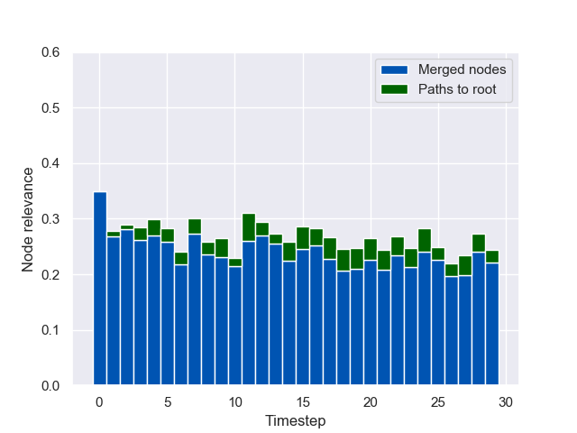
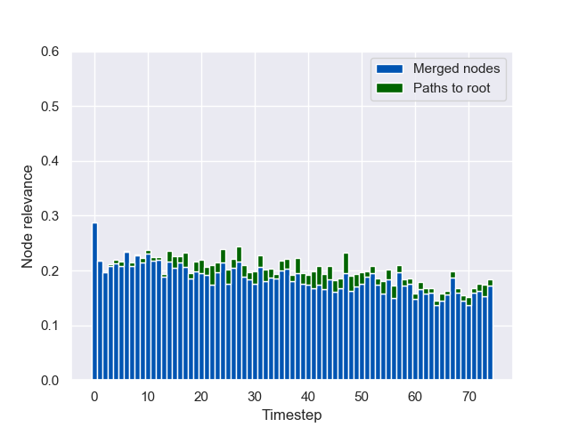
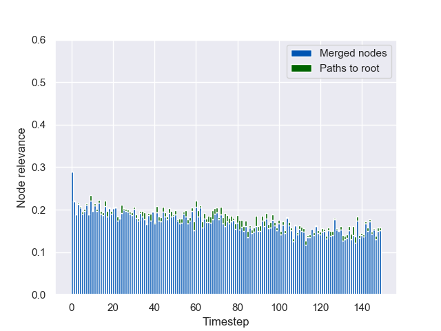
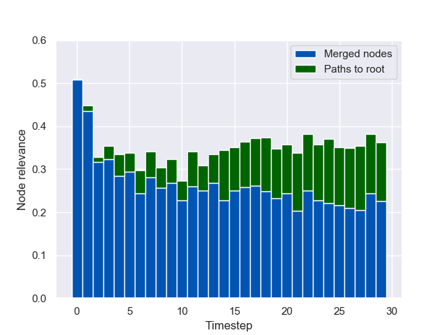
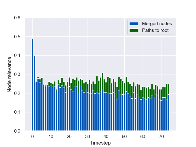
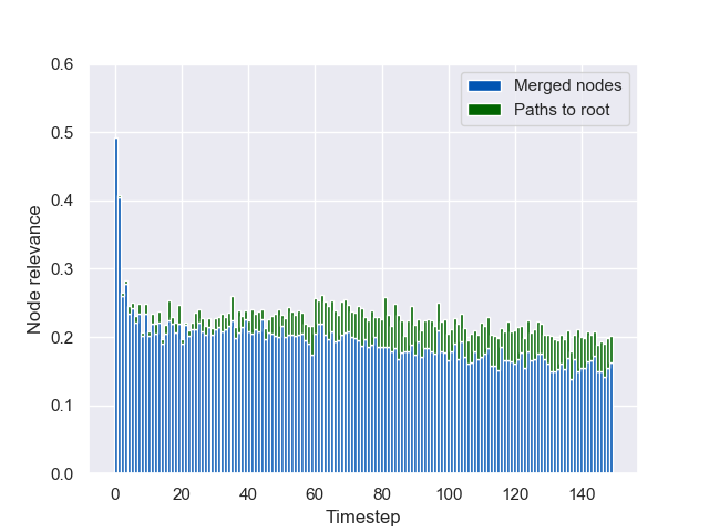
Figure 8: Credit assignment study results for the DSU setup, for the baseline GNN (Top) and the PGN (Bottom), arranged left-to-right by test graph size. PGNs learn to put larger emphasis on both the two nodes being operated on (blue) and the nodes on their respective paths-to-roots (green).

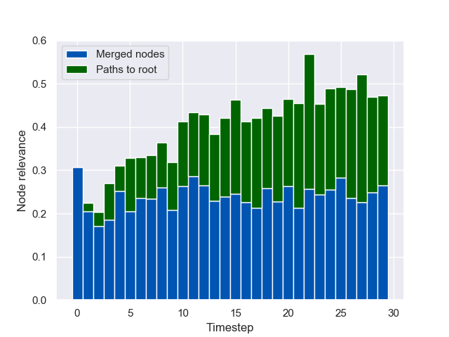
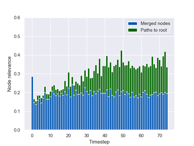
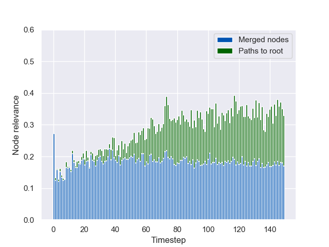
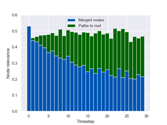
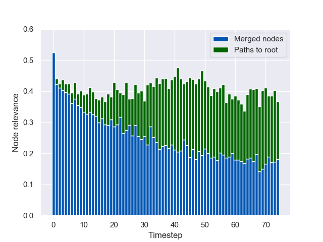
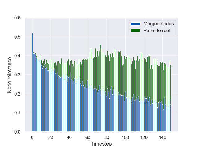
Figure 9: Credit assignment study results for the LCT setup, following same convention as Figure 8.

Firstly, recall how our decoder network, $g$, is applied to the latent state ($\vec{z}_{i}^{(t)}$, $\vec{h}_{i}^{(t)}$), in order to derive predicted query answers, $\vec{y}_{i}^{(t)}$ (Equation 3). Knowing that the elementwise maximisation aggregator performed the best as aggregation function, we can rewrite Equation 3 as follows:

$$\vec{y}^{(t)}=g\left(\max_{i}\vec{z}_{i}^{(t)},\max_{i}\vec{h}_{i}^{(t)}\right)$$ (9)

This form of max-pooling readout has a unique feature: each dimension of the input vectors to $g$ will be contributed to by exactly one node (the one which optimises the corresponding dimension in $\vec{z}_{i}^{(t)}$ or $\vec{h}_{i}^{(t)}$). This provides us with opportunity to perform a credit assignment study: we can verify how often every node has propagated its features into this vector—and hence, obtain a direct estimate of how “useful” this node is for the decision making by any of our considered models.

We know from the direct analysis of disjoint-set union (Section 3) and link/cut tree (Appendix C) operations that only a subset of the nodes are directly involved in decision-making for dynamic connectivity. These are exactly the nodes along the paths from $u$ and $v$, the two nodes being operated on, to their respective roots in the data structure. Equivalently, these nodes directly correspond to the nodes tagged by ground-truth masks (nodes $i$ for which $\hat{\mu}_{i}^{(t)}=0$).

With the above hindsight, we compare a trained baseline GNN model against a PGN model, in terms of how much credit is assigned to these “important” nodes, throughout the rollout. The results of this study are visualised in Figures 8 (for DSU) and 9 (for LCT), visualising separately the credit assigned to the two nodes being operated on (blue) and the remaining nodes along their paths-to-roots (green).

From these plots, we can make several direct observations:

• In all settings, the PGN amplifies the overall credit assigned to these relevant nodes.

• On the DSU setup, the baseline GNN is likely suffering from oversmoothing effects: at larger test set sizes, it seems to hardly distinguish the paths-to-root (which are often very short due to path compression) from the remainder of the neighbourhoods. The PGN explicitly encodes the inductive bias of the structure, and hence more explicitly models such paths.

• As ground-truth LCT pointers are not amenable to path compression, paths-to-root may more significantly grow in lengthwith graph size increase. Hence at this point the oversmoothing effect is less pronounced for baselines; but in this case, LCT operations are highly centered on the node being operated on. The PGN learns to provide additional emphasis to the nodes operated on, $u$ and $v$.

In all cases, it appears that through a careful and targeted constructed graph, the PGN is able to significantly overcome the oversmoothing issues with fully-connected GNNs, providing further encouragement for applying PGNs in problem settings where strong credit assignment is required, one example of which are search problems.

References

- [1] Peter Battaglia, Razvan Pascanu, Matthew Lai, Danilo Jimenez Rezende, et al. Interaction networks for learning about objects, relations and physics. In Advances in neural information processing systems, pages 4502–4510, 2016.
- [2] James Bradbury, Roy Frostig, Peter Hawkins, Matthew James Johnson, Chris Leary, Dougal Maclaurin, and Skye Wanderman-Milne. JAX: composable transformations of Python+NumPy programs, 2018.
- [3] Deli Chen, Yankai Lin, Wei Li, Peng Li, Jie Zhou, and Xu Sun. Measuring and relieving the over-smoothing problem for graph neural networks from the topological view. arXiv preprint arXiv:1909.03211, 2019.
- [4] Zhengdao Chen, Lei Chen, Soledad Villar, and Joan Bruna. Can graph neural networks count substructures? arXiv preprint arXiv:2002.04025, 2020.
- [5] Thomas H Cormen, Charles E Leiserson, Ronald L Rivest, and Clifford Stein. Introduction to algorithms. MIT press, 2009.
- [6] Andreea Deac, Pierre-Luc Bacon, and Jian Tang. Graph neural induction of value iteration. arXiv preprint arXiv:2009.12604, 2020.
- [7] Efim A Dinic. Algorithm for solution of a problem of maximum flow in networks with power estimation. In Soviet Math. Doklady, volume 11, pages 1277–1280, 1970.
- [8] Vijay Prakash Dwivedi, Chaitanya K Joshi, Thomas Laurent, Yoshua Bengio, and Xavier Bresson. Benchmarking graph neural networks. arXiv preprint arXiv:2003.00982, 2020.
- [9] Luca Franceschi, Mathias Niepert, Massimiliano Pontil, and Xiao He. Learning discrete structures for graph neural networks. arXiv preprint arXiv:1903.11960, 2019.
- [10] Michael Fredman and Michael Saks. The cell probe complexity of dynamic data structures. In Proceedings of the twenty-first annual ACM symposium on Theory of computing, pages 345–354, 1989.
- [11] Bernard A Galler and Michael J Fisher. An improved equivalence algorithm. Communications of the ACM, 7(5):301–303, 1964.
- [12] Vikas K Garg, Stefanie Jegelka, and Tommi Jaakkola. Generalization and representational limits of graph neural networks. arXiv preprint arXiv:2002.06157, 2020.
- [13] Dobrik Georgiev and Pietro Lió. Neural bipartite matching. arXiv preprint arXiv:2005.11304, 2020.
- [14] Justin Gilmer, Samuel S Schoenholz, Patrick F Riley, Oriol Vinyals, and George E Dahl. Neural message passing for quantum chemistry. arXiv preprint arXiv:1704.01212, 2017.
- [15] Ashish Goel, Sanjeev Khanna, Daniel H Larkin, and Robert E Tarjan. Disjoint set union with randomized linking. In Proceedings of the twenty-fifth annual ACM-SIAM symposium on Discrete algorithms, pages 1005–1017. SIAM, 2014.
- [16] Aditya Grover, Aaron Zweig, and Stefano Ermon. Graphite: Iterative generative modeling of graphs. arXiv preprint arXiv:1803.10459, 2018.
- [17] Jessica B Hamrick, Kelsey R Allen, Victor Bapst, Tina Zhu, Kevin R McKee, Joshua B Tenenbaum, and Peter W Battaglia. Relational inductive bias for physical construction in humans and machines. arXiv preprint arXiv:1806.01203, 2018.
- [18] Tom Hennigan, Trevor Cai, Tamara Norman, and Igor Babuschkin. Haiku: Sonnet for JAX, 2020.
- [19] Bo Jiang, Ziyan Zhang, Doudou Lin, Jin Tang, and Bin Luo. Semi-supervised learning with graph learning-convolutional networks. In Proceedings of the IEEE Conference on Computer Vision and Pattern Recognition, pages 11313–11320, 2019.
- [20] Łukasz Kaiser and Ilya Sutskever. Neural gpus learn algorithms. arXiv preprint arXiv:1511.08228, 2015.
- [21] Anees Kazi, Luca Cosmo, Nassir Navab, and Michael Bronstein. Differentiable graph module (dgm) graph convolutional networks. arXiv preprint arXiv:2002.04999, 2020.
- [22] Diederik P Kingma and Jimmy Ba. Adam: A method for stochastic optimization. arXiv preprint arXiv:1412.6980, 2014.
- [23] Thomas Kipf, Ethan Fetaya, Kuan-Chieh Wang, Max Welling, and Richard Zemel. Neural relational inference for interacting systems. arXiv preprint arXiv:1802.04687, 2018.
- [24] Nikita Kitaev, Łukasz Kaiser, and Anselm Levskaya. Reformer: The efficient transformer. arXiv preprint arXiv:2001.04451, 2020.
- [25] Wouter Kool, Herke van Hoof, and Max Welling. Attention, learn to solve routing problems! arXiv preprint arXiv:1803.08475, 2018.
- [26] Joseph B Kruskal. On the shortest spanning subtree of a graph and the traveling salesman problem. Proceedings of the American Mathematical society, 7(1):48–50, 1956.
- [27] Yujia Li, Oriol Vinyals, Chris Dyer, Razvan Pascanu, and Peter Battaglia. Learning deep generative models of graphs. arXiv preprint arXiv:1803.03324, 2018.
- [28] Meng Liu, Zhengyang Wang, and Shuiwang Ji. Non-local graph neural networks. arXiv preprint arXiv:2005.14612, 2020.
- [29] Sitao Luan, Mingde Zhao, Xiao-Wen Chang, and Doina Precup. Break the ceiling: Stronger multi-scale deep graph convolutional networks. In Advances in Neural Information Processing Systems, pages 10943–10953, 2019.
- [30] Ryan L Murphy, Balasubramaniam Srinivasan, Vinayak Rao, and Bruno Ribeiro. Janossy pooling: Learning deep permutation-invariant functions for variable-size inputs. arXiv preprint arXiv:1811.01900, 2018.
- [31] Alexander Pritzel, Benigno Uria, Sriram Srinivasan, Adria Puigdomenech Badia, Oriol Vinyals, Demis Hassabis, Daan Wierstra, and Charles Blundell. Neural episodic control. In Proceedings of the 34th International Conference on Machine Learning-Volume 70, pages 2827–2836. JMLR. org, 2017.
- [32] JZ Qiu, Jian Tang, Hao Ma, YX Dong, KS Wang, and J Tang. Deepinf: Modeling influence locality in large social networks. In Proceedings of the 24th ACM SIGKDD International Conference on Knowledge Discovery and Data Mining (KDD’18), 2018.
- [33] Oliver Richter and Roger Wattenhofer. Normalized attention without probability cage. arXiv preprint arXiv:2005.09561, 2020.
- [34] Alvaro Sanchez-Gonzalez, Jonathan Godwin, Tobias Pfaff, Rex Ying, Jure Leskovec, and Peter W Battaglia. Learning to simulate complex physics with graph networks. arXiv preprint arXiv:2002.09405, 2020.
- [35] Adam Santoro, David Raposo, David G Barrett, Mateusz Malinowski, Razvan Pascanu, Peter Battaglia, and Timothy Lillicrap. A simple neural network module for relational reasoning. In Advances in neural information processing systems, pages 4967–4976, 2017.
- [36] Hadar Serviansky, Nimrod Segol, Jonathan Shlomi, Kyle Cranmer, Eilam Gross, Haggai Maron, and Yaron Lipman. Set2graph: Learning graphs from sets. arXiv preprint arXiv:2002.08772, 2020.
- [37] Yossi Shiloach and Shimon Even. An on-line edge-deletion problem. Journal of the ACM (JACM), 28(1):1–4, 1981.
- [38] Daniel D Sleator and Robert Endre Tarjan. A data structure for dynamic trees. Journal of computer and system sciences, 26(3):362–391, 1983.
- [39] Richard P Stanley. Acyclic orientations of graphs. In Classic Papers in Combinatorics, pages 453–460. Springer, 2009.
- [40] Hao Tang, Zhiao Huang, Jiayuan Gu, Baoliang Lu, and Hao Su. Towards Scale-Invariant Graph-related Problem Solving by Iterative Homogeneous GNNs. The 34th Annual Conference on Neural Information Processing Systems (NeurIPS), 2020.
- [41] Robert E Tarjan and Jan Van Leeuwen. Worst-case analysis of set union algorithms. Journal of the ACM (JACM), 31(2):245–281, 1984.
- [42] Robert E Tarjan and Renato F Werneck. Dynamic trees in practice. Journal of Experimental Algorithmics (JEA), 14:4–5, 2010.
- [43] Robert Endre Tarjan. Efficiency of a good but not linear set union algorithm. Journal of the ACM (JACM), 22(2):215–225, 1975.
- [44] Robert Endre Tarjan and Uzi Vishkin. Finding biconnected componemts and computing tree functions in logarithmic parallel time. In 25th Annual Symposium onFoundations of Computer Science, 1984., pages 12–20. IEEE, 1984.
- [45] Andrew Trask, Felix Hill, Scott E Reed, Jack Rae, Chris Dyer, and Phil Blunsom. Neural arithmetic logic units. In Advances in Neural Information Processing Systems, pages 8035–8044, 2018.
- [46] Ashish Vaswani, Noam Shazeer, Niki Parmar, Jakob Uszkoreit, Llion Jones, Aidan N Gomez, Łukasz Kaiser, and Illia Polosukhin. Attention is all you need. In Advances in neural information processing systems, pages 5998–6008, 2017.
- [47] Petar Veličković, Rex Ying, Matilde Padovano, Raia Hadsell, and Charles Blundell. Neural execution of graph algorithms. arXiv preprint arXiv:1910.10593, 2019.
- [48] Petar Veličković, Guillem Cucurull, Arantxa Casanova, Adriana Romero, Pietro Liò, and Yoshua Bengio. Graph attention networks. arXiv preprint arXiv:1710.10903, 1(2), 2017.
- [49] Oriol Vinyals, Samy Bengio, and Manjunath Kudlur. Order matters: Sequence to sequence for sets. arXiv preprint arXiv:1511.06391, 2015.
- [50] Oriol Vinyals, Meire Fortunato, and Navdeep Jaitly. Pointer networks. In Advances in Neural Information Processing Systems, pages 2692–2700, 2015.
- [51] Guangtao Wang, Rex Ying, Jing Huang, and Jure Leskovec. Improving graph attention networks with large margin-based constraints. arXiv preprint arXiv:1910.11945, 2019.
- [52] Yue Wang, Yongbin Sun, Ziwei Liu, Sanjay E Sarma, Michael M Bronstein, and Justin M Solomon. Dynamic graph cnn for learning on point clouds. ACM Transactions on Graphics (TOG), 38(5):1–12, 2019.
- [53] Keyulu Xu, Weihua Hu, Jure Leskovec, and Stefanie Jegelka. How powerful are graph neural networks? arXiv preprint arXiv:1810.00826, 2018.
- [54] Keyulu Xu, Jingling Li, Mozhi Zhang, Simon S Du, Ken-ichi Kawarabayashi, and Stefanie Jegelka. What can neural networks reason about? arXiv preprint arXiv:1905.13211, 2019.
- [55] Yujun Yan, Kevin Swersky, Danai Koutra, Parthasarathy Ranganathan, and Milad Heshemi. Neural execution engines: Learning to execute subroutines. arXiv preprint arXiv:2006.08084, 2020.
- [56] Manzil Zaheer, Satwik Kottur, Siamak Ravanbakhsh, Barnabas Poczos, Russ R Salakhutdinov, and Alexander J Smola. Deep sets. In Advances in neural information processing systems, pages 3391–3401, 2017.
- [57] Wojciech Zaremba and Ilya Sutskever. Learning to execute. arXiv preprint arXiv:1410.4615, 2014.
- [58] Lingxiao Zhao and Leman Akoglu. Pairnorm: Tackling oversmoothing in gnns. arXiv preprint arXiv:1909.12223, 2019.