STL-SGD: Speeding Up Local SGD with Stagewise Communication Period

Abstract

Distributed parallel stochastic gradient descent algorithms are workhorses for large scale machine learning tasks. Among them, local stochastic gradient descent (Local SGD) has attracted significant attention due to its low communication complexity. Previous studies prove that the communication complexity of Local SGD with a fixed or an adaptive communication period is in the order of $O(N^{\frac{3}{2}}T^{\frac{1}{2}})$ and $O(N^{\frac{3}{4}}T^{\frac{3}{4}})$ when the data distributions on clients are identical (IID) or otherwise (Non-IID), where $N$ is the number of clients and $T$ is the number of iterations. In this paper, to accelerate the convergence by reducing the communication complexity, we propose STagewise Local SGD (STL-SGD), which increases the communication period gradually along with decreasing learning rate. We prove that STL-SGD can keep the same convergence rate and linear speedup as mini-batch SGD. In addition, as the benefit of increasing the communication period, when the objective is strongly convex or satisfies the Polyak-Łojasiewicz condition, the communication complexity of STL-SGD is $O(N\log{T})$ and $O(N^{\frac{1}{2}}T^{\frac{1}{2}})$ for the IID case and the Non-IID case respectively, achieving significant improvements over Local SGD. Experiments on both convex and non-convex problems demonstrate the superior performance of STL-SGD.

Introduction

We consider the task of distributed stochastic optimization, which employs $N$ clients to solve the following empirical risk minimization problem:

$$\min_{x\in R^{d}}f(x):=\frac{1}{N}\sum_{i=1}^{N}f_{i}(x),$$ (1)

where $f_{i}(x):=\frac{1}{|\mathcal{D}_{i}|}\sum_{\xi\in\mathcal{D}_{i}}f(x,\xi)$ is the local objective of client $i$. $\mathcal{D}_{i}$’s denote the data distributions among clients, which can be possibly different. Specifically, the scenario where $\mathcal{D}_{i}$’s are identical corresponds to a central problem of traditional distributed optimization. When they are not identical, (1) captures the federated learning setting (McMahan et al. 2017; Kairouz et al. 2019; Lyu, Yu, and Yang 2020), where the local data in each mobile client is independent and private, resulting in high variance of the data distributions.

As representatives of distributed stochastic optimization methods, traditional Synchronous SGD (SyncSGD) (Dekel et al. 2012; Ghadimi and Lan 2013) and Asynchronous SGD (AsyncSGD) (Agarwal and Duchi 2011; Lian et al. 2015) achieve linear speedup theoretically with respect to the number of clients. Nevertheless, for both SyncSGD and AsyncSGD, communication needs to be conducted at each iteration and $O(d)$ parameters are communicated each time, incurring significant communication cost which restricts the performance in terms of time speedup. To address this dilemma, distributed algorithms with low communication cost, either by decreasing the communication frequency (Wang and Joshi 2018b; Stich 2019; Yu, Yang, and Zhu 2019; Shen et al. 2019) or by reducing the communication bits in each round (Alistarh et al. 2017; Stich, Cordonnier, and Jaggi 2018; Tang et al. 2019), become widely applied for large scale training.

Among them, Local SGD (Stich 2019) (also called FedAvg (McMahan et al. 2017)), which conducts communication every $k$ iterations, enjoys excellent theoretical and practical performance (Lin et al. 2018; Stich 2019). In the IID case and the Non-IID case, the communication complexity of Local SGD is respectively proved to be $O(N^{\frac{3}{2}}T^{\frac{1}{2}})$ (Wang and Joshi 2018b; Stich 2019) and $O(N^{\frac{3}{4}}T^{\frac{3}{4}})$ (Yu, Yang, and Zhu 2019; Shen et al. 2019), while the linear speedup is maintained. When the objective satisfies the Polyak-Łojasiewicz condition (Karimi, Nutini, and Schmidt 2016), (Haddadpour et al. 2019a) provides a tighter theoretical analysis which shows that the communication complexity of Local SGD is $O(N^{\frac{1}{3}}T^{\frac{1}{3}})$. In terms of the communication period $k$, most previous studies of Local SGD choose to fix it through the iterations. In contrast, (Wang and Joshi 2018a) suggests using an adaptively decreasing $k$ when the learning rate is fixed, and (Haddadpour et al. 2019a) proposes an adaptively increasing $k$ as the iterations go on. Nevertheless, none of them achieve a communication complexity lower than $O(N^{\frac{1}{3}}T^{\frac{1}{3}})$. For strongly convex objectives, if a fixed learning rate is adopted, Local SGD with fixed communication period is proved to achieve $O(N\log{(NT)})$ (Stich and Karimireddy 2019; Bayoumi, Mishchenko, and Richtarik 2020) communication complexity. However, the fixed learning rate results in suboptimal convergence rate $O(\frac{\log{T}}{NT})$. It remains an open problem as to whether the communication complexity can be further reduced with a varying $k$ when the optimal convergence rate $O(\frac{1}{NT})$ is maintained, to which this paper provides an affirmative solution.

Main Contributions. We propose Stagewise Local SGD (STL-SGD), which adopts a stagewisely increasing communication period , and make the following contributions:

• We first prove that Local SGD achieves $O(\frac{1}{\sqrt{NT}})$ convergence when the objective is general convex. A novel insight is that, the convergence rate $O(\frac{1}{\sqrt{NT}})$ can be attained when setting $k$ to be $O(\frac{1}{\eta N})$ and $O(\frac{1}{\sqrt{\eta N}})$ in the IID case and the Non-IID case respectively, where $\eta$ is the learning rate. This indicates that the communication period is negatively relevant to the learning rate.

• Taking Local SGD as a subalgorithm and tuning its parameters stagewisely, we propose $\text{STL-SGD}^{sc}$ for strongly convex problems, which geometrically increases the communication period along with decreasing learning rate. We prove that $\text{STL-SGD}^{sc}$ achieves $O(\frac{1}{NT})$ convergence rate with communication complexities $O(N\log{T})$ and $O(N^{\frac{1}{2}}T^{\frac{1}{2}})$ for the IID case and the Non-IID case, respectively.

• For non-convex problems, we propose the $\text{STL-SGD}^{nc}$ algorithm, which uses Local SGD to optimize a regularized objective $f_{x_{s}}^{\gamma}(\cdot)$ inexactly at each stage. When the Polyak-Łojasiewicz condition holds, the same communication complexity as in strongly convex problems is achieved. For general non-convex problems, we prove that $\text{STL-SGD}^{nc}$ achieves the linear speedup with communication complexities $O(N^{\frac{3}{2}}T^{\frac{1}{2}})$ and $O(N^{\frac{3}{4}}T^{\frac{3}{4}})$ for the IID case and the Non-IID case, respectively.

Table 1: A comparison of the results in this paper and previous state-of-the-art results of Local SGD and its variants. Regarding orders of convergence rate and communication complexity, we highlight the dependency on $T$ (the number of iterations), $N$ (the number of clients) and $k$ (communication period). Previous results may depend on some extra assumptions, which include: (1) an upper bound for gradient, (2) an upper bound for the gradient variance among clients and (3) an upper bound for the gradient diversity, which are shown in the last column.

Algorithms	Objectives	Convergence Rate	Communication Complexity	Data Distributions	Extra Assumptions
Local SGD (Stich 2019)	Strongly Convex	$O(\frac{1}{NT})$	$O(N^{\frac{1}{2}}T^{\frac{1}{2}})$	IID	(1)
Local SGD (Stich and Karimireddy 2019)	Strongly Convex	$O(\frac{\log{T}}{NT})$	$O(N\log{(NT)})$	IID	No
STL-SGD	Strongly Convex	$O(\frac{1}{NT})$	$O(N\log{T})$	IID	No
Local SGD (Li et al. 2020)	Strongly Convex	$O(\frac{k^{2}}{NT})$	$O(T)$	Non-IID	(1)
Local SGD (Karimireddy et al. 2019)	Strongly Convex	$O(\frac{\log{T}}{NT})$	$O(N^{\frac{1}{2}}T^{\frac{1}{2}})$	Non-IID	No
SCAFFOLD (Karimireddy et al. 2019)	Strongly Convex	$O(\frac{\log{T}}{NT})$	$O(\log{(NT)})$	Non-IID	No
STL-SGD	Strongly Convex	$O(\frac{1}{NT})$	$O(N^{\frac{1}{2}}T^{\frac{1}{2}})$	Non-IID	No
Local SGD (Haddadpour et al. 2019a)	Non-Convex+PL	$O(\frac{1}{NT})$	$O(N^{\frac{1}{3}}T^{\frac{1}{3}})$	IID	No
STL-SGD	Non-Convex+PL	$O(\frac{1}{NT})$	$O(N\log{T})$	IID	No
STL-SGD	Non-Convex+PL	$O(\frac{1}{NT})$	$O(N^{\frac{1}{2}}T^{\frac{1}{2}})$	Non-IID	No
Local SGD (Wang and Joshi 2018b)	Non-Convex	$O(\frac{1}{\sqrt{NT}})$	$O(N^{\frac{3}{2}}T^{\frac{1}{2}})$	IID	(1)
STL-SGD	Non-Convex	$O(\frac{1}{\sqrt{NT}})$	$O(N^{\frac{3}{2}}T^{\frac{1}{2}})$	IID	No
Local SGD (Shen et al. 2019)	Non-Convex	$O(\frac{1}{\sqrt{NT}})$	$O(N^{\frac{3}{4}}T^{\frac{3}{4}})$	Non-IID	(2)
Local SGD (Haddadpour and Mahdavi 2019)	Non-Convex	$O(\frac{1}{\sqrt{NT}})$	$O(N^{\frac{3}{2}}T^{\frac{1}{2}})$	Non-IID	(3)
SCAFFOLD (Karimireddy et al. 2019)	Non-Convex	$O(\frac{1}{\sqrt{NT}})$	$O(N^{\frac{1}{2}}T^{\frac{1}{2}})$	Non-IID	No
STL-SGD	Non-Convex	$O(\frac{1}{\sqrt{NT}})$	$O(N^{\frac{3}{4}}T^{\frac{3}{4}})$	Non-IID	No

Related Works

Local SGD.

When the data distributions on clients are identical, Local SGD is proved to achieve $O(\frac{1}{NT})$ convergence for strongly convex objectives (Stich 2019) and $O(\frac{1}{\sqrt{NT}})$ convergence for non-convex objectives (Wang and Joshi 2018b) when the communication period $k$ satisfies $k\leq O(T^{\frac{1}{2}}/N^{\frac{3}{2}})$. As demonstrated in these results, Local SGD achieves a linear speedup with the communication complexity $O(N^{\frac{3}{2}}T^{\frac{1}{2}})$ for both strongly convex and non-convex objectives in the IID case. In addition, (Haddadpour et al. 2019a) justifies that $O(N^{\frac{1}{3}}T^{\frac{1}{3}})$ rounds of communication are sufficient to achieve $O(\frac{1}{NT})$ convergence for objectives which satisfy the Polyak-Łojasiewicz condition. On the other hand, for the Non-IID case, Local SGD is proved with a $O(1/\sqrt{NT})$ convergence rate under a communication complexity of $O(N^{\frac{3}{4}}T^{\frac{3}{4}})$ for non-convex objectives (Yu, Yang, and Zhu 2019; Shen et al. 2019). Meanwhile, for strongly convex objectives, a suboptimal convergence rate of $O(\frac{k^{2}}{\mu NT})$ (Li et al. 2020) is obtained. Beyond that, when a small fixed learning rate is adopted, (Bayoumi, Mishchenko, and Richtarik 2020) and (Karimireddy et al. 2019) prove that the communication complexity of Local SGD is $O(N\log(NT))$ and $O(N^{\frac{1}{2}}T^{\frac{1}{2}})$ for the IID case and the Non-IID case respectively, at the cost of a suboptimal convergence rate $O(\frac{\log{T}}{NT})$. For general non-convex objectives, (Haddadpour and Mahdavi 2019) proves a lower communication complexity of $O(N^{\frac{3}{2}}T^{\frac{1}{2}})$ for the Non-IID case under the assumption of bounded gradient diversity. From the practical view, (Zhang et al. 2016) suggests to communicate more frequently in the beginning of the training, and (Haddadpour et al. 2019a) verifies that using a geometrically increasing period does not harm the convergence notably.

Stagewise Training.

For training both strongly convex and non-convex objectives, stagewisely decreasing the learning rate is widely adopted. Epoch-SGD (Hazan and Kale 2014) and ASSG (Xu, Lin, and Yang 2017) use SGD as their subalgorithm and geometrically decrease the learning rate stage by stage. They are proved to achieve the optimal $O(1/T)$ convergence for stochastic strongly convex optimization. For training neural networks, stagewisely decreasing the learning rate (Krizhevsky, Sutskever, and Hinton 2012; He et al. 2016) is a very important trick. From a theoretical aspect, stagewise SGD is proved with $O(1/\sqrt{T})$ convergence for both general and composite non-convex objectives (Allen-Zhu 2018; Chen et al. 2019; Davis and Grimmer 2019), by adopting SGD to optimize a regularized objective at each stage and decreasing the learning rate linearly stage by stage. Stagewise training is also verified to achieve better testing error than general SGD (Yuan et al. 2019).

Large Batch SGD (LB-SGD).

SyncSGD with extremely large batch is proved to achieve a linear speedup with respect to the batch size (Stich and Karimireddy 2019). Nevertheless, (Jain et al. 2016) shows that increasing the batch size does not help when the bias dominates the variance. It is also observed from practice that LB-SGD leads to a poor generalization (Keskar et al. 2016; Golmant et al. 2018; Yin et al. 2017). (Yu and Jin 2019) proposes CR-PSGD which increases the batch size geometrically step by step and proves that CR-PSGD achieves a linear speedup with $O(\log{T})$ communication complexity. However, after a large number of iterations, CR-PSGD essentially becomes GD and loses the benefit of SGD.

Local SGD with Variance Reduction.

Recently, several techniques are proposed to reduce the communication complexity of Local SGD in the Non-IID case. (Haddadpour et al. 2019b) shows that using redundant data among clients yields lower communication complexity. One variant of Local SGD called VRL-SGD (Liang et al. 2019) incorporates the variance reduction technique and is proved to achieve a $O(N^{\frac{3}{2}}T^{\frac{1}{2}})$ communication complexity for non-convex objectives. SCAFFOLD (Karimireddy et al. 2019) extends VRL-SGD by involving two separate learning rates, and is proved to achieve $O(\log{(NT)})$ and $O(N^{\frac{1}{2}}T^{\frac{1}{2}})$ communication complexities for strongly convex objectives and non-convex objectives respectively. As SCAFFOLD adopts a small fixed learning rate, its convergence rate for strongly convex objectives is $O(\frac{\log{T}}{NT})$. Nevertheless, these methods are orthogonal to our study. Combining STL-SGD and variance reduction to get better performance for the Non-IID case exceeds the scope of this paper.

Table 1 summarizes the comparison of Local SGD and its state-of-the-art extensions with STL-SGD. For both strongly convex objectives and non-convex objectives which satisfy the PL condition, STL-SGD achieves the state-of-the-art communication complexity while attaining the optimal convergence rate of $O(\frac{1}{NT})$. It is worth mentioning that Local SGD with momentum (Yu, Jin, and Yang 2019) or adaptive learning rate (Reddi et al. 2020) are orthogonal to our study.

Preliminaries

Notations and Definitions

Throughout the paper, we let $\|\cdot\|$ indicate the $\ell_{2}$ norm of a vector and $\langle\cdot,\cdot\rangle$ indicate the inner product of two vectors. The set $\{1,2,\cdots,n\}$ is denoted as $[n]$. We use $x^{*}$ to represent the optimal solution of (1). $\nabla f$ represents the gradient of $f$. $\mathbb{E}$ indicates a full expectation with respect to all the randomness in the algorithm (the stochastic gradients sampled in all iterations and the randomness in return).

The data distributions on different clients may not be identical. To quantify the difference of distributions, we define $\zeta_{f}^{*}:=\frac{1}{N}\sum_{i=1}^{N}\|\nabla f_{i}(x^{*})\|^{2}=\frac{1}{N}\sum_{i=1}^{N}\|\nabla f_{i}(x^{*})-\nabla f(x^{*})\|^{2}$, which represents the variance of gradients among clients at $x^{*}$. Some literatures assume that the variance of gradients among clients is bounded by a constant $\zeta^{2}$ (Shen et al. 2019) or the norm of stochastic gradients is bounded by a constant $G^{2}$ (Yu, Yang, and Zhu 2019; Li et al. 2020). Note that both $\zeta^{2}$ and $G^{2}$ are larger than $\zeta_{f}^{*}$. When the data distributions are identical, we have $\|\nabla f_{i}(x^{*})\|^{2}=0$, thus it holds that $\zeta_{f}^{*}=0$.

All proofs are deffered to the appendix. To state the convergence of algorithms for solving (1), we introduce some commonly used definitions (Chen et al. 2019; Haddadpour et al. 2019a).

Definition 1 ($\rho$-weakly convex).

A non-convex function $f(x)$ is $\rho$-weakly convex ($\rho>0$) if

$$f(x)\geq f(y)+\langle\nabla f(y),x-y\rangle-\frac{\rho}{2}\|x-y\|^{2},\forall x,y\in R^{d}.$$

Definition 2 ($\mu$-Polyak-Łojasiewicz (PL)).

A function $f(x)$ satisfies the $\mu$-PL condition ($\mu>0$) if

$$2\mu(f(x)-f(x^{*}))\leq\|\nabla f(x)\|^{2},\forall x\in R^{d}.$$

Assumptions

Throughout this paper, we make the following assumptions, all of which are commonly used and basic assumptions (Stich 2019; Yu, Yang, and Zhu 2019; Li et al. 2020; Chen et al. 2019; Allen-Zhu 2018).

Assumption 1.

$f_{i}(x)$ is $L$-smooth in terms of $i\in[N]$ for every $x\in R^{d}$:

$$\|\nabla f_{i}(x)-\nabla f_{i}(y)\|\leq L\|x-y\|,\forall x,y\in R^{d},i\in[N].$$

Assumption 2.

There exists a constant $\sigma$ such that

$$\mathbb{E}_{\xi\sim\mathcal{D}_{i}}\|\nabla f(x,\xi)-\nabla f_{i}(x)\|^{2}\leq\sigma^{2},\forall x\in R^{d},\forall i\in[N].$$

Assumption 3.

If the objective function is non-convex, we assume it is $\rho$-weakly convex.

Remark 1.

Note that if $f(x)$ is $L$-smooth, it is $L$-weakly convex. This is because Assumption 1 implies $-\frac{L}{2}\|x-y\|^{2}\leq f(x)-f(y)-\langle\nabla f(y),x-y\rangle\leq\frac{L}{2}\|x-y\|^{2}$ (Nesterov 2018). Therefore, for an $L$-smooth function, we can immediately get that the weakly-convex parameter $\rho$ satisfies $0<\rho\leq L$.

Review: Synchronous SGD with Periodically Averaging (Local SGD)

To alleviate the high communication cost in SyncSGD, the periodically averaging technique is proposed (Stich 2019; Yu, Yang, and Zhu 2019). Instead of averaging models in all clients at every iteration, Local SGD lets clients update their models locally for $k$ iterations, then one communication is conducted to average the local models to make them consistent. Specifically, the update rule of Local SGD is

$$x_{t}^{i}=\begin{cases}\frac{1}{N}\sum_{j=1}^{N}(x_{t-1}^{j}-\eta\nabla f(x_{t-1}^{j},\xi_{t-1}^{j})),&{\textrm{if}~{}t~{}\%~{}k~{}=~{}0},\\ x_{t-1}^{i}-\eta\nabla f(x_{t-1}^{i},\xi_{t-1}^{i}),&{\textrm{else}},\end{cases}$$

where $x_{t}^{i}$ is the local model in client $i$ at iteration $t$. Therefore, when each client conducts $T$ iterations, the total number of communications is $T/k$. The complete procedure of Local SGD is summarized in Algorithm 1. Different from previous studies (McMahan et al. 2017; Stich 2019; Yu, Yang, and Zhu 2019), Algorithm 1 returns $\tilde{x}=\frac{1}{N}\sum_{i=1}^{N}x_{t}^{i}$ for a randomly chosen $t\in\{0,1,\cdots,T-1\}$. In practice, we can determine $t$ at first to avoid redundant iterations.

Algorithm 1 Local-SGD($f$, $x_{0}$, $\eta$, $T$, $k$)

Initialize: $x_{0}^{i}=x_{0},\forall i\in[N].$

1:  for $t=1,...,T$ do

2:     Client $C_{i}$ does:

3:     Uniformly sample a mini-batch $\xi_{t-1}^{i}\in\mathcal{D}_{i}$ and calculate a stochastic gradient $\nabla f_{i}(x_{t-1}^{i},\xi_{t-1}^{i})$.

4:     if $t$ divides $k$ then

5:        Communicate with other clients and update: $x_{t}^{i}=\sum_{j=1}^{N}\frac{1}{N}(x_{t-1}^{j}-\eta\nabla f(x_{t-1}^{j},\xi_{t-1}^{j}))$.

6:     else

7:        Update locally: $x_{t}^{i}=x_{t-1}^{i}-\eta\nabla f_{i}(x_{t-1}^{i},\xi_{t-1}^{i})$.

8:     end if

9:  end for

10:  return $\tilde{x}=\frac{1}{N}\sum_{i=1}^{N}x_{t}^{i}$ for the randomly chosen $t\in\{0,1,\cdots,T-1\}$.

Although several studies have analysed the convergence of Local SGD, they assume that the objective $f(x)$ is $\mu$-strongly convex or non-convex. (Khaled, Mishchenko, and Richtárik 2019) focuses on general convex objectives while they use the full gradient descent. Besides, most of the existing analysis relies on some stronger assumptions, including bounded gradient norm (i.e., $\|\nabla f_{i}(x,\xi)\|^{2}\leq G^{2}$) (Stich 2019; Li et al. 2020) or bounded variance of gradients among clients (Shen et al. 2019). Here, we give a basic convergence result of Local SGD for the general convex objectives without these assumptions.

Theorem 1.

Suppose Assumptions 1 and 2 hold, $f(x)$ is convex and $\eta\leq\frac{1}{6L}$. If we set $k\leq\min\{\frac{1}{6\eta LN},\frac{1}{9\eta L}\}$ and $k\leq\min\{\frac{\sigma}{\sqrt{6\eta LN(\sigma^{2}+4\zeta_{f}^{*})}},\frac{1}{9\eta L}\}$ for the IID case and the Non-IID case respectively, we have

$$\mathbb{E}f(\tilde{x})-f(x^{*})\leq\frac{3\|x_{0}-x^{*}\|^{2}}{4\eta T}+\frac{\eta\sigma^{2}}{N}.$$ (2)

Remark 2.

If we set $\eta=\sqrt{\frac{N}{T}}$, we have $\mathbb{E}f(\tilde{x})-f(x^{*})\leq\frac{\|x_{0}-x^{*}\|^{2}+\sigma^{2}}{\sqrt{NT}}$, which is consistent with the result of mini-batch SGD (Dekel et al. 2012).

Local SGD with Stagewise Communication Period

To further reduce the communication complexity, we propose STagewise Local SGD (STL-SGD) in this section with the following features.

• At the beginning, STL-SGD employs Algorithm 1 as a subalgorithm in each stage.

• Instead of using a small fixed learning rate or a gradually decreasing learning rate (e.g. $\frac{\eta_{1}}{1+\alpha t}$), STL-SGD adopts a stagewisely adaptive scheme. The learning rate is fixed at first, and decreased stage by stage.

• The communication periods are increased stagewisely.

We propose two variants of STL-SGD for strongly convex and non-convex problems, respectively.

STL-SGD for Strongly Convex Problems

Algorithm 2 $\text{STL-SGD}^{sc}$($f$, $x_{1}$, $\eta_{1}$, $T_{1}$, $k_{1}$)

1:  for $s=1,2,...,S$ do

2:     $x_{s+1}$ = Local-SGD($f$, $x_{s}$, $\eta_{s}$, $T_{s}$, $\max\{\lfloor k_{s}\rfloor,1\}$).

3:     Set $\eta_{s+1}=\frac{\eta_{s}}{2}$, $T_{s+1}=2T_{s}$ and

$$k_{s+1}=\begin{cases}\sqrt{2}k_{s},~{}~{}~{}{\rm Non\text{-}IID~{}case},\\ 2k_{s},~{}~{}~{}~{}~{}~{}{\rm IID~{}case}.\end{cases}$$

4:  end for

5:  return $x_{S+1}$.

In this subsection, we propose the STL-SGD algorithm for strongly convex problems, which is denoted as $\text{STL-SGD}^{sc}$ and summarized in Algorithm 2. At each stage, the learning rate is decreased exponentially. In the meantime, the number of iterations and the communication period are increased exponentially. Specifically, at the $s$-th stage, we set $\eta_{s}=\frac{\eta_{s-1}}{2}$ and $T_{s}=2T_{s-1}$. The communication period $k_{s}$ is set as $k_{s}=2k_{s-1}$ and $k_{s}=\sqrt{2}k_{s-1}$ for the IID case and the Non-IID case respectively.

Below, let $x_{s}$ denote the initial point of the $s$-th stage. Theorem 2 establishes the convergence rate of $\text{STL-SGD}^{sc}$.

Theorem 2.

Suppose $f(x)$ is $\mu$-strongly convex. Let $\eta_{1}\leq\frac{1}{6L}$ and $T_{1}\eta_{1}=\frac{6}{\mu}$. We set $k_{1}=\min\{\frac{1}{6\eta_{1}LN},\frac{1}{9\eta_{1}L}\}$ and $k_{1}=\min\{\frac{\sigma}{\sqrt{6\eta_{1}LN(\sigma^{2}+4\zeta_{f})}},\frac{1}{9\eta_{1}L}\}$ for the IID case and the Non-IID case respectively. Under Assumptions 1 and 2, when the number of stages satisfies $S\geq\log(\frac{N(f(x_{0})-f(x^{*}))}{\eta_{1}\sigma^{2}})+2$, we have the following result for Algorithm 2:

$$\mathbb{E}f(x_{S+1})-f(x^{*})\leq\frac{9\eta_{1}\sigma^{2}}{2^{S}N}.$$ (3)

Defining $T:=T_{1}+T_{2}+\cdots+T_{S}$, we have

$$\mathbb{E}f(x_{S+1})-f(x^{*})\leq O\left(\frac{1}{NT}\right).$$ (4)

Remark 3.

Theorem 2 claims the following properties of $\text{STL-SGD}^{sc}$:

• Linear Speedup. To reach a solution $x_{S+1}$ with $\mathbb{E}f(x_{S+1})-f(x^{*})\leq\epsilon$, the number of iterations is $O(\frac{1}{N\epsilon})$, which indicates a linear speedup.

• Communication Complexity for the Non-IID Case. For the Non-IID case, we set $k_{s+1}=\sqrt{2}k_{s}$ for Algorithm 2. Therefore, the total communication complexity is $\frac{T_{1}}{k_{1}}+\cdots+\frac{T_{S}}{k_{S}}=\frac{T_{1}}{k_{1}}(1+2^{\frac{1}{2}}+\cdots+2^{\frac{s-1}{2}})=O(\frac{T_{1}}{k_{1}}\cdot(\frac{T}{T_{1}})^{\frac{1}{2}})=O(N^{\frac{1}{2}}T^{\frac{1}{2}})$, where the last equality holds because $\frac{T_{1}^{\frac{1}{2}}}{k_{1}}=O(\sqrt{T_{1}\eta_{1}N})=O(N^{\frac{1}{2}})$.

• Communication Complexity for the IID Case. If the data distributions on different clients are identical, we set $k_{s+1}=2k_{s}$ for Algorithm 2. Thus, the total communication complexity is $\frac{T_{1}}{k_{1}}+\cdots+\frac{T_{S}}{k_{S}}=S\frac{T_{1}}{k_{1}}=O(N\log{T})$.

STL-SGD for Non-Convex Problems

Algorithm 3 $\text{STL-SGD}^{nc}$($f$, $x_{1}$, $\eta_{1}$, $T_{1}$, $k_{1}$)

1:  for $s=1,2,...,S$ do

2:     Let $f_{x_{s}}^{\gamma}(x)=f(x)+\frac{1}{2\gamma}\|x-x_{s}\|^{2}$.

3:     $x_{s+1}$ = Local-SGD($f_{x_{s}}^{\gamma}$, $x_{s}$, $\eta_{s}$, $T_{s}$, $\max\{\lfloor k_{s}\rfloor,1\}$).

4:     Option 1: Set $\eta_{s+1}=\frac{\eta_{s}}{2}$, $T_{s+1}=2T_{s}$ and

$$k_{s+1}=\begin{cases}\sqrt{2}k_{s},~{}~{}~{}~{}~{}~{}~{}{\rm Non\text{-}IID~{}case},\\ 2k_{s},~{}~{}~{}~{}~{}~{}~{}~{}~{}~{}{\rm IID~{}~{}case}.\end{cases}$$

5:     Option 2: Set $\eta_{s+1}=\frac{\eta_{1}}{s+1}$, $T_{s+1}=(s+1)T_{1}$ and

$$k_{s+1}=\begin{cases}\sqrt{s+1}k_{1},~{}~{}~{}~{}~{}~{}~{}{\rm Non\text{-}IID~{}case},\\ (s+1)k_{1},~{}~{}~{}~{}~{}~{}~{}{\rm IID~{}case}.\end{cases}$$

6:  end for

7:  return $x_{S+1}$.

In this subsection, we proceed to propose the variant of STL-SGD algorithm for non-convex problems ($\text{STL-SGD}^{nc}$). Different from Algorithm 2, which optimizes a fixed objective during all stages, $\text{STL-SGD}^{nc}$ changes the objective once a stage is finished. Specifically, in the $s$-th stage, the objective is a regularized problem $f_{x_{s}}^{\gamma}=f(x)+\frac{1}{2\gamma}\|x-x_{s}\|^{2}$, where $x_{s}$ is the initial point of the $s$-th stage and $\gamma$ is a constant that satisfies $\gamma<\rho^{-1}$. $f_{x_{s}}^{\gamma}(x)$ is guaranteed to be convex due to the $\rho$-weak convexity of $f(x)$. In this way, the theoretical property of Algorithm 1 under convex settings still holds in each stage of $\text{STL-SGD}^{nc}$. Other parameters are set in two different ways (Option 1 and Option 2) for non-convex objectives satisfying the PL condition and otherwise, which are detailed in Algorithm 3.

In Option 1, we set $\eta_{s}$, $T_{s}$ and $k_{s}$ in the same way as in Algorithm 2. Here we analyse the theoretical property of $\text{STL-SGD}^{nc}$ with Option 1 for non-convex objectives that satisfy the PL condition.

Theorem 3.

Assume $f(x)$ satisfies the PL condition defined in Definition 2 with constant $\mu$. Suppose Assumptions 1, 2 and 3 hold and $f(x)$ is weakly convex with constant $\rho\leq\frac{\mu}{16}$. Let $\eta_{1}\leq\frac{1}{12L_{\gamma}}$, $T_{1}\eta_{1}=\frac{6}{\rho}$. Set $k_{1}=\min\{\frac{1}{6\eta_{1}L_{\gamma}N},\frac{1}{9\eta_{1}L_{\gamma}}\}$ and $k_{1}=\min\{\frac{\sigma}{\sqrt{6\eta_{1}L_{\gamma}N(\sigma^{2}+4\zeta_{f})}},\frac{1}{9\eta_{1}L_{\gamma}}\}$ for the IID case and the Non-IID case respectively. When the number of stages satisfies $S\geq\log{\frac{N\left(f(x_{0})-f(x^{*})\right)}{\eta_{1}\sigma^{2}}}+2$, Algorithm 3 with Option 1 returns a solution $x_{S+1}$ such that

$$\mathbb{E}f(x_{S+1})-f(x^{*})\leq O\left(\frac{1}{NT}\right),$$ (5)

where $T=T_{1}+T_{2}+\cdots+T_{S}$.

Remark 4.

As the result of Theorem 3 is the same as that of Theorem 2, properties stated in Remark 3 all hold here.

Option 2 is employed for the non-convex objectives which do not satisfy the PL condition. Instead of increasing the communication period geometrically as in Option 1 of Algorithm 3, we let it increase in a linear manner, i.e., $k_{s}=sk_{1}$. Meanwhile, we increase the stage length linearly, that is $T_{s}=sT_{1}$, while keeping $T_{s}\eta_{s}$ a constant.

Theorem 4.

Suppose Assumptions 1, 2 and 3 hold. Let $\eta_{1}\leq\frac{1}{6L_{\gamma}}$ and $T_{1}\eta_{1}=\frac{3}{\rho}$. Set $k_{1}=\min\{\frac{1}{6\eta_{1}LN},\frac{1}{9\eta_{1}L}\}$ and $k_{1}=\min\{\frac{\sigma}{\sqrt{6\eta_{1}LN(\sigma^{2}+4\zeta_{f})}},\frac{1}{9\eta_{1}L}\}$ for the IID case and the Non-IID case respectively. Algorithm 3 with Option 2 guarantees that

$$\mathbb{E}\|\nabla f(x_{s})\|^{2}\leq O\left(\frac{1}{\sqrt{NT}}\right),$$ (6)

where $s$ is randomly sampled from $\{1,2,\cdots,S\}$ with probability $p_{s}=\frac{s}{1+2+\cdots+S}$.

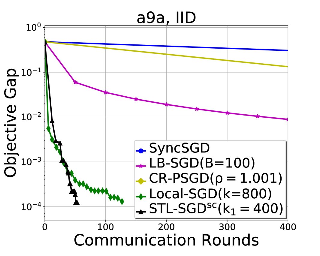
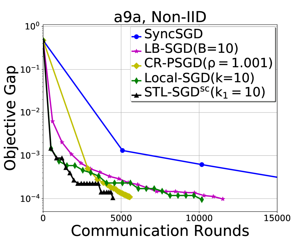
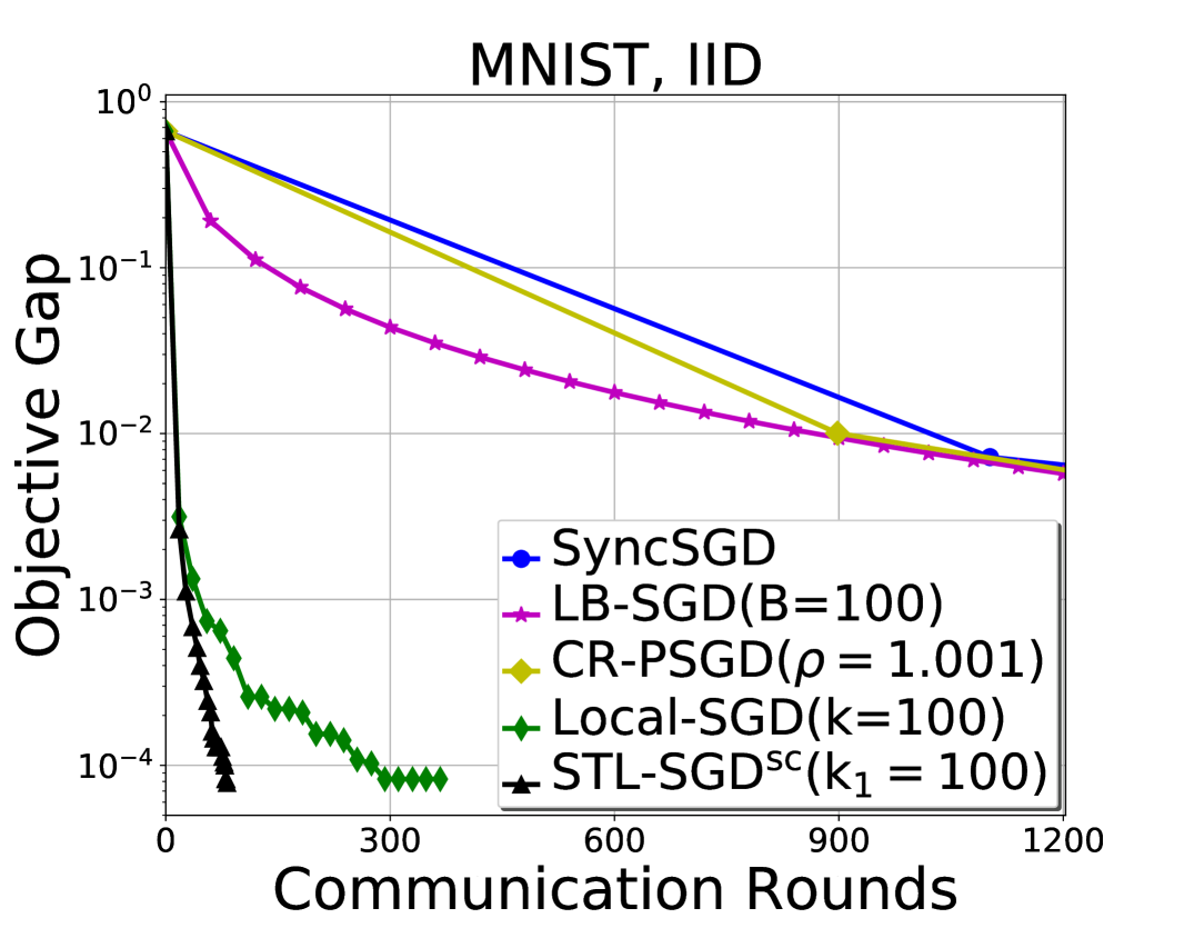
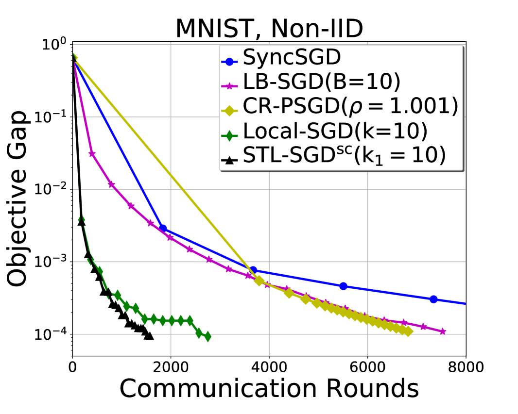
Figure 1: Training objective gap $f(x)-f(x^{*})$ w.r.t the communication rounds for logistic regression on $\mathrm{a9a}$ and $\mathrm{MNIST}$.

Table 2: Communication rounds to reach $10^{-4}$ objective gap in convex problems. We also show the speedup of these algorithms compared with SyncSGD.

Algorithms	a9a (IID)	a9a (Non-IID)	MNIST (IID)	MNIST (Non-IID)
SyncSGD	100683 ($1\times$)	90513 ($1\times$)	32664 ($1\times$)	22021 ($1\times$)
LB-SGD	7620     ($13.2\times$)	12221 ($7.4\times$)	7011   ($4.7\times$)	7740   ($2.8\times$)
CR-PSGD	5434     ($18.5\times$)	5772   ($15.7\times$)	6788   ($4.8\times$)	7029   ($3.1\times$)
Local-SGD	184       ($547.2\times$)	10068 ($9.0\times$)	289     ($113.0\times$)	2642   ($8.3\times$)
$\text{STL-SGD}^{sc}$	61         ($1650.5\times$)	4417   ($20.5\times$)	79       ($413.5\times$)	1518   ($14.5\times$)

Remark 5.

$\text{STL-SGD}^{nc}$ with Option 2 has the following properties:

• Linear Speedup: To achieve $\mathbb{E}\|\nabla f(x_{S})\|^{2}\leq\epsilon$, the total number of iterations when $N$ clients are used is $O(\frac{1}{N\epsilon^{2}})$, which shows a linear speedup.

• Communication Complexity for the Non-IID case: Algorithm 3 with Option 2 sets $k_{s}=\sqrt{s}k_{1}$. Thus, the communication complexity is $\frac{T_{1}}{k_{1}}+\frac{T_{2}}{k_{2}}+\cdots+\frac{T_{S}}{k_{S}}=\frac{T_{1}}{k_{1}}(1+\sqrt{2}+\cdots+\sqrt{S})=O(\frac{T_{1}}{k_{1}}(\frac{T}{T_{1}})^{\frac{3}{4}})=O(N^{\frac{3}{4}}T^{\frac{3}{4}})$.

• Communication Complexity for the IID case: As $k_{s}=sk_{1}$, the communication complexity is $\frac{T_{1}}{k_{1}}+\frac{T_{2}}{k_{2}}+\cdots+\frac{T_{S}}{k_{S}}=\frac{T_{1}}{k_{1}}S=O(\frac{T_{1}}{k_{1}}(\frac{T}{T_{1}})^{\frac{1}{2}})=O\left(N^{\frac{3}{2}}T^{\frac{1}{2}}\right)$.

Experiments

We validate the performance of the proposed STL-SGD algorithm with experiments on both convex and non-convex problems. For each type of problems, we conduct experiments for both the IID case and the Non-IID case. Experiments are conducted on a machine with 8 Nvidia Geforce GTX 1080Ti GPUs and 2 Xeon(R) Platinum 8153 CPUs.

To simulate the Non-IID scenarios, we divide the training data and make the distributions of classes different among clients. Similar to the setting in (Karimireddy et al. 2019), at first, we randomly take $s\%$ i.i.d. data from the training set and divide them equally to each client. For the remaining data, we sort them according to their classes and then assign them to the clients in order. In our experiments, we set $s=50$ for convex problems and $s=0$ for non-convex problems.

We compare STL-SGD with SyncSGD, LB-SGD, CR-PSGD (Yu and Jin 2019) and Local SGD (Stich 2019). We show the comparison of these algorithms in terms of the communication rounds. The investigation regarding convergence is included in the appendix, which validates that STL-SGD can achieve similar convergence rate as SyncSGD.

Convex Problems

We consider the binary classification problem with logistic regression, i.e.,

$$\min_{\theta\in R^{d}}\frac{1}{n}\sum_{i=1}^{n}\log(1+\exp(-y_{i}x_{i}^{T}\theta))+\frac{\lambda}{2}\|\theta\|^{2},$$ (7)

where $(x_{i},y_{i}),i\in[n]$ constitute a set of training examples, and $\lambda$ is the regularization parameter. It is notable that (7) is strongly convex when $\lambda>0$, and we set $\lambda=1/n$. We take two datasets $\mathrm{a9a}$ and $\mathrm{MNIST}$ from the libsvm website. $\mathrm{a9a}$ has $32,561$ examples and $123$ features. For $\mathrm{MNIST}$, we sample a subset with $11,791$ examples and $784$ features from two classes (4 and 9). Experiments are implemented on 32 clients and communication is handled with MPI.

SyncSGD, LB-SGD and Local SGD are implemented with the decreasing learning rate $\eta_{t}=\frac{\eta_{1}}{1+\alpha t}$ as suggested in (Stich 2019; Li et al. 2020) and we tune $\alpha$ in $\{10^{-2},10^{-3},10^{-4}\}$ for the best performance. For $\text{STL-SGD}^{sc}$, we set $\eta_{1}T_{1}=\frac{1}{\lambda}$. The initial learning rate for all algorithms is tuned in $\{N,N/10,N/100\}$. The communication period $k$ and the batch size $B$ for LB-SGD are tuned in $\{100,200,400,800,1600\}$ for the IID case, and $\{10,20,40,80,160\}$ for the Non-IID case. The scaling factor of batch size $\rho$ for CR-PSGD is tuned in $\{1.001,1.01,1.1\}$. We report the largest $k$, $B$ and $\rho$ which do not sacrifice the convergence for all algorithms.

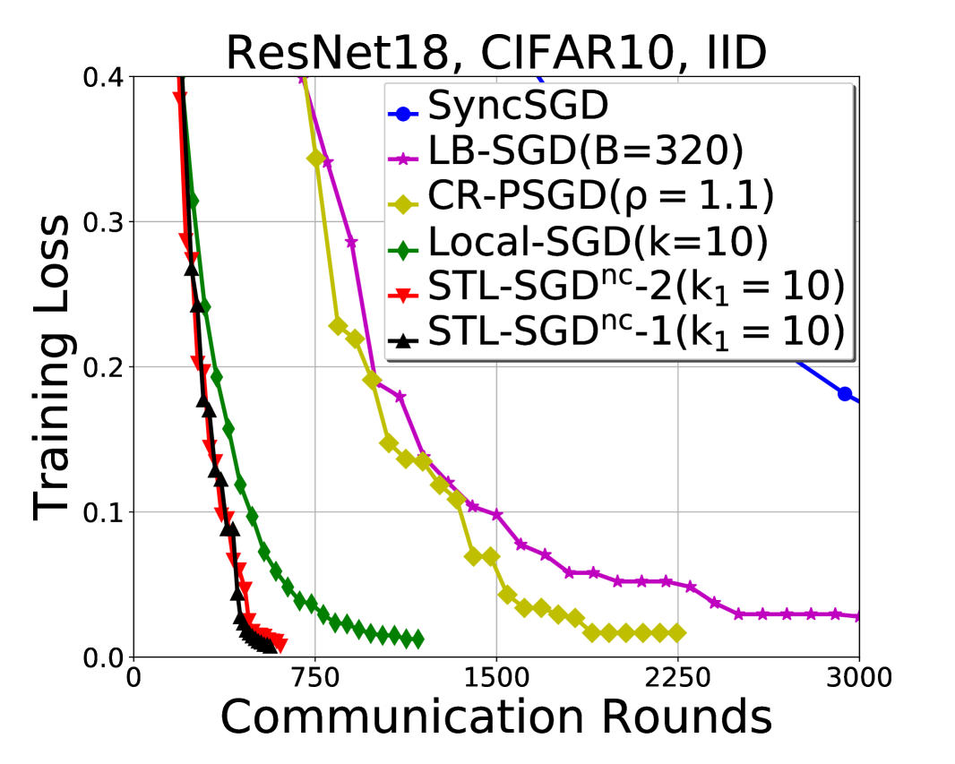
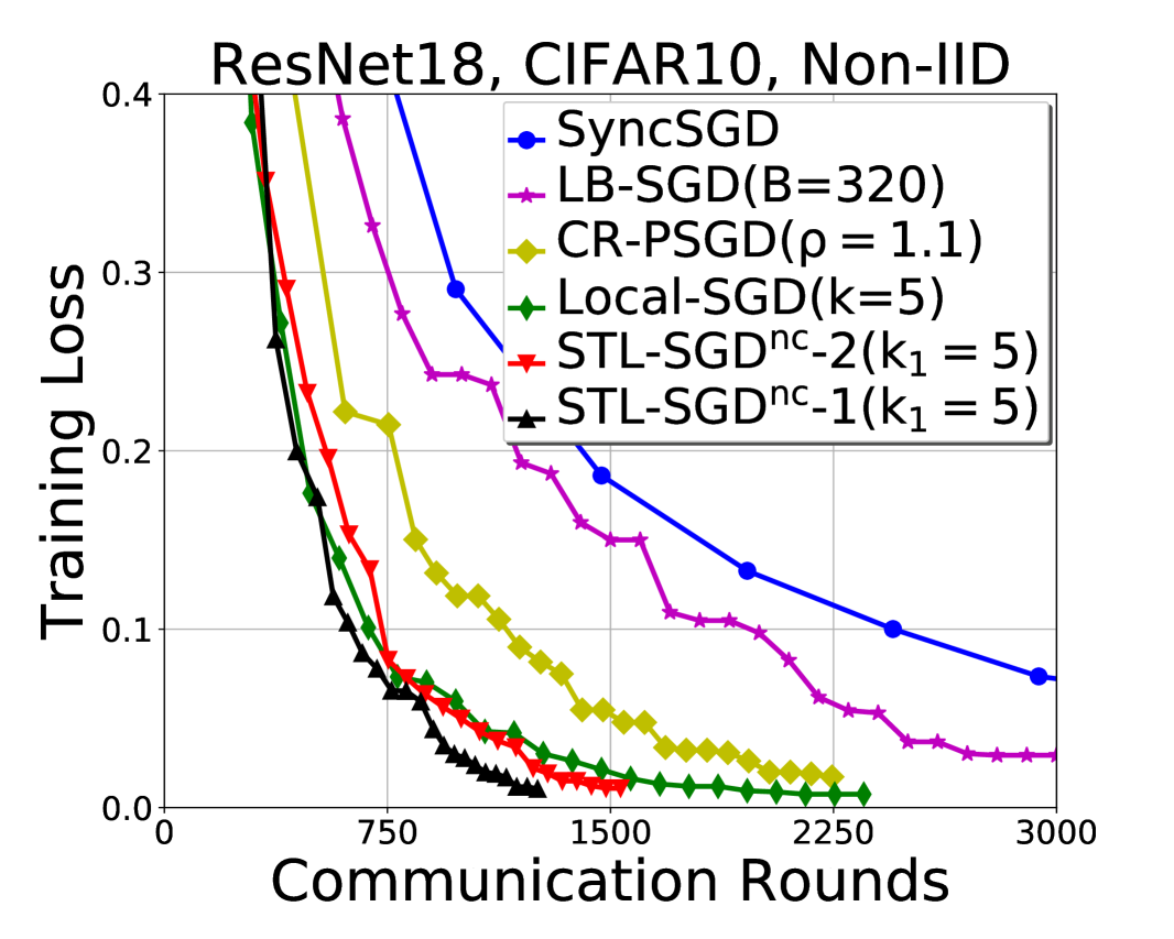
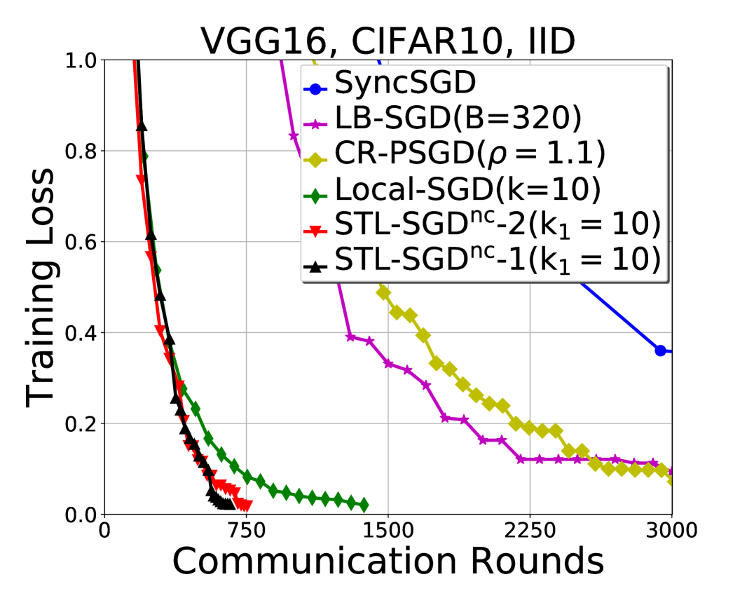
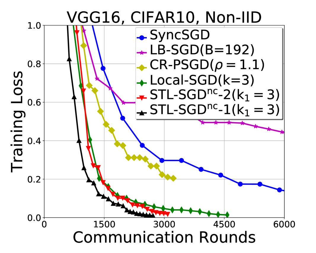
Figure 2: Training loss w.r.t the communication rounds for ResNet18 and VGG16 on CIFAR10.

Table 3: Communication rounds to reach 99% training accuracy in non-convex problems. We run all algorithms for 200 epochs, where an epoch indicates one pass of the dataset. LB-SGD and CR-PSGD can not achieve 99% training accuracy on the VGG16 neural network until the end of training.

Algorithms	ResNet18 (IID)	ResNet18 (Non-IID)	VGG16 (IID)	VGG16 (Non-IID)
SyncSGD	7644 ($1\times$)	5390 ($1\times$)	13622 ($1\times$)	15092 ($1\times$)
LB-SGD	3000 ($2.5\times$)	3180 ($1.7\times$)	$-$        ($-$)	$-$        ($-$)
CR-PSGD	1797 ($4.3\times$)	1937 ($2.8\times$)	$-$        ($-$)	$-$        ($-$)
Local-SGD	755   ($10.1\times$)	1235 ($4.4\times$)	1245   ($10.9\times$)	3986   ($3.8\times$)
$\text{STL-SGD}^{nc}$-2	470   ($16.3\times$)	1158 ($4.7\times$)	696     ($19.6\times$)	2732   ($5.5\times$)
$\text{STL-SGD}^{nc}$-1	434   ($17.6\times$)	954   ($5.6\times$)	602     ($22.6\times$)	2179   ($6.9\times$)

Figure 1 shows the objective gap $f(x)-f(x^{*})$ with regard to the communication rounds. We can observe that $\text{STL-SGD}^{sc}$ converges with the fewest communication rounds for both the IID case and the Non-IID case. Although the initial communication period of $\text{STL-SGD}^{sc}$ may need to be set smaller than Local SGD in the the IID case, the total number of communication rounds of $\text{STL-SGD}^{sc}$ is still significantly lower, which validates that the communication complexity of $\text{STL-SGD}^{sc}$ is much lower than Local SGD. As shown in Table 2, to achieve $10^{-4}$ objective gap, the communication rounds of $\text{STL-SGD}^{sc}$ is almost 1.7-3 times fewer than Local SGD.

Non-Convex Problems

We train ResNet18 (He et al. 2016) and VGG16 (Simonyan and Zisserman 2014) on the $\mathrm{CIFAR10}$ (Krizhevsky, Hinton et al. 2009) dataset, which includes a training set of 50,000 examples from 10 classes. 8 clients are used in total.

For our proposed algorithm, we denote $\text{STL-SGD}^{nc}$ with Option 1 and Option 2 as $\text{STL-SGD}^{nc}$-1 and $\text{STL-SGD}^{nc}$-2 respectively. The learning rates of SyncSGD, LB-SGD, CR-PSGD and Local-SGD are all set fixed as suggested in their convergence theory (Ghadimi and Lan 2013; Yu and Jin 2019; Yu, Yang, and Zhu 2019). The initial learning rate for all algorithms is tuned in $\{N/10,N/100,N/1000\}$. The basic batch size at each client is 64. The first stage length of $\text{STL-SGD}^{nc}$ is tuned in $\{20,40,60\}$ epochs. The parameter $\gamma$ in $\text{STL-SGD}^{nc}$ is tuned in $\{10^{0},10^{2},10^{4}\}$. We tune the communication period $k$ in $\{3,5,10,20\}$ and the batch size $B$ for LB-SGD in $\{192,320,640,1280\}$. For ease of implementation, we increase the batch size in CR-PSGD with $B=\rho B$ once an epoch is finished, and $\rho$ is tuned in $\{1.1,1.2,1.3\}$. $B$ stops growing when it exceeds $512$ as suggested in (Yu and Jin 2019). We show the largest $k$ and $B$ which can maintain the same convergence rate as SyncSGD for all algorithms.

The experimental results of training loss regarding communication rounds are presented in Figure 2 and the communication rounds to achieve 99% training accuracy for all algorithms are shown in Table 3. As can be seen, $\text{STL-SGD}^{nc}$-1 and $\text{STL-SGD}^{nc}$-2 converge with much fewer communications than other algorithms. In spite of the same order of communication complexity as Local SGD, the performance of $\text{STL-SGD}^{nc}$-2 is better as the benefit of the negative relevance between the learning rate and the communication period. $\text{STL-SGD}^{nc}$-1 converges with the fewest number of communications, as it uses a geometrically increasing communication period.

Conclusion

We propose STL-SGD, which adopts a stagewisely increasing communication period to reduce the communication complexity. Two variants of STL-SGD ($\text{STL-SGD}^{sc}$ and $\text{STL-SGD}^{nc}$) are provided for strongly convex objectives and non-convex objectives respectively. Theoretically, we prove that: (i) STL-SGD maintains the convergence rate and linear speedup as SyncSGD; (ii) when the objective is strongly convex or satisfies the PL condition, while attaining the optimal convergence rate $O(\frac{1}{NT})$, STL-SGD achieves the state-of-the-art communication complexity; (iii) when the objective is general non-convex, STL-SGD has the same communication complexity as Local SGD, while being more consistent with practical tricks. Experiments on both convex and non-convex problems demonstrate the effectiveness of the proposed algorithm.

Aknowledgement

This research was supported by the National Natural Science Foundation of China (61673364) and Anhui Provincial Natural Science Foundation (2008085J31). We would like to thank the Information Science Laboratory Center of USTC for the hardware and software services. We also gratefully acknowledge Xianfeng Liang from USTC for his valuable discussion.

Appendix A More About Experiments

Experimental Results for Validating the Convergence Rate

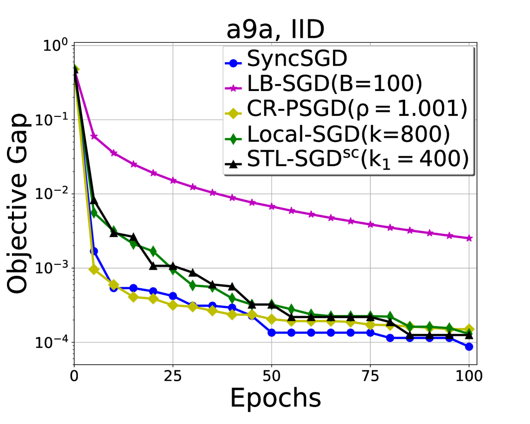
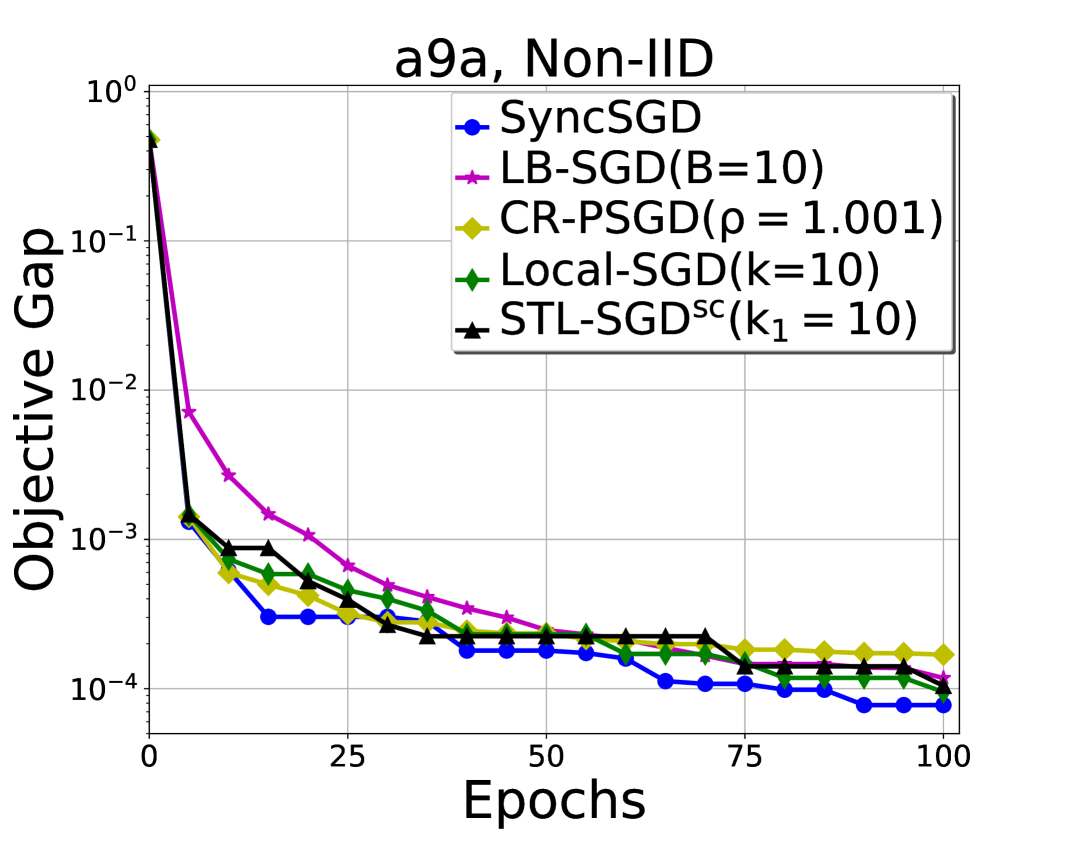
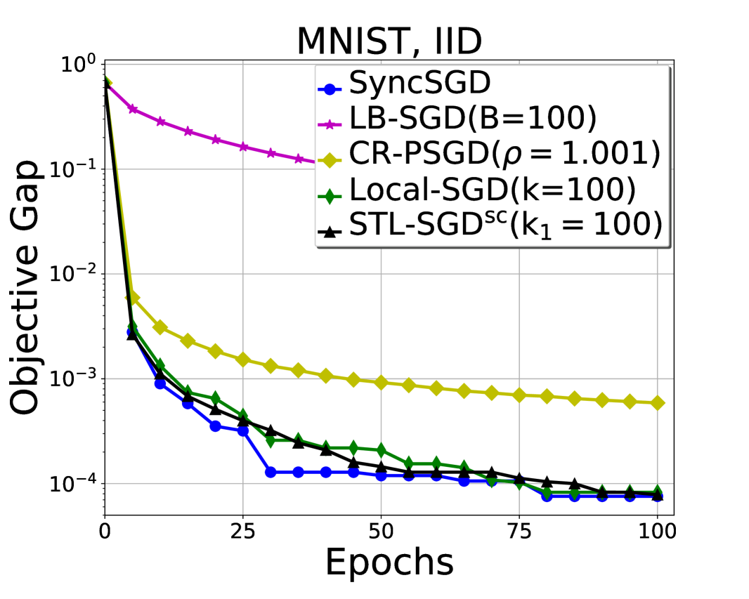
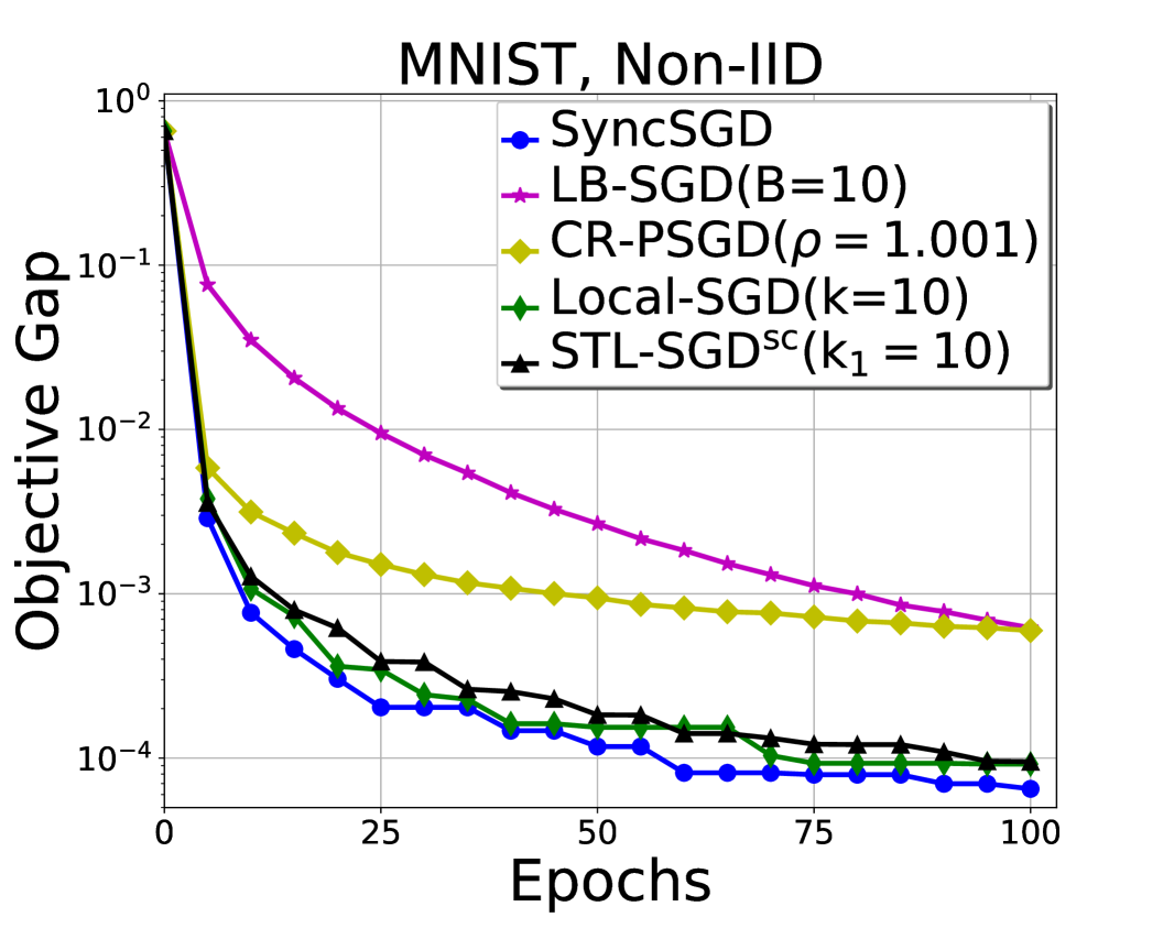
Figure 3: Training objective gap $f(x)-f(x^{*})$ w.r.t epochs for logistic regression on $\mathrm{a9a}$ and MNIST datasets.

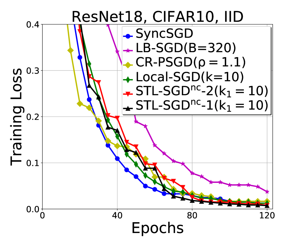
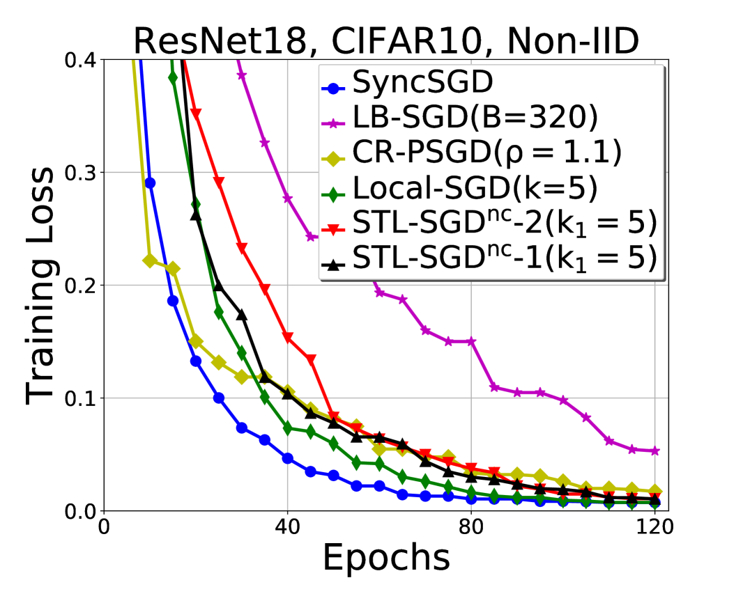
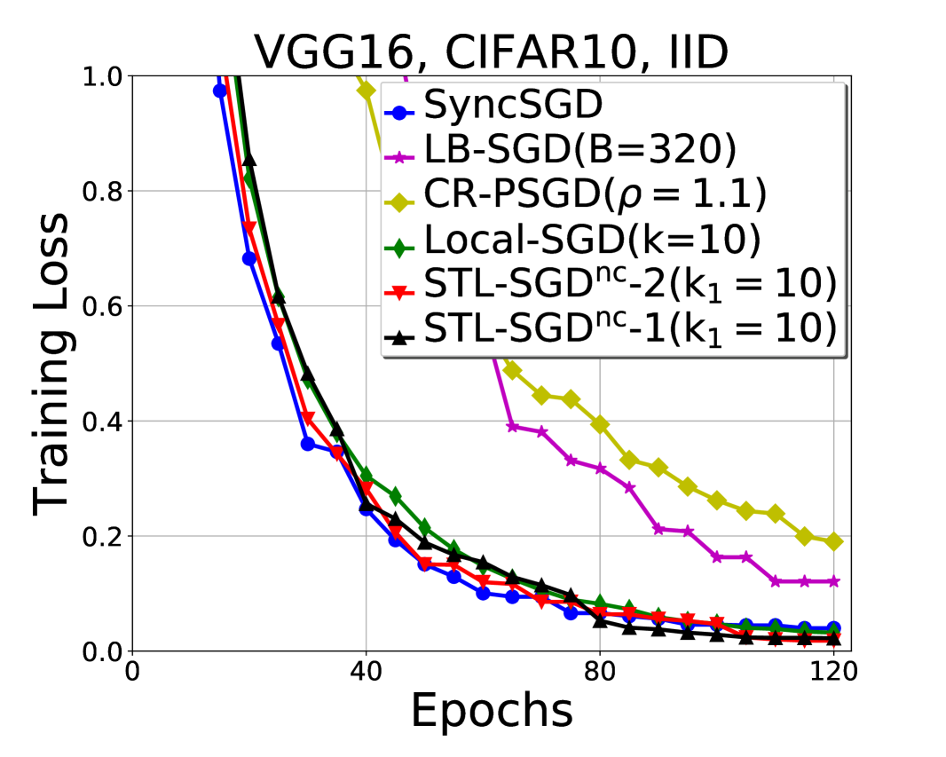
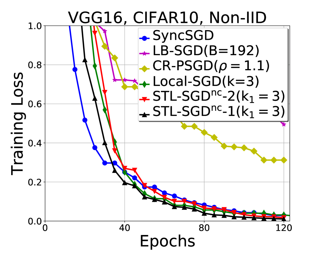
Figure 4: Training loss w.r.t epochs for ResNet18 and VGG16 on CIFAR10 dataset.

In this subsection, we supplement the experimental results not included in the main paper. The rules for turning the hyper-parameters are presented in Subsection Experiments and we turn all hyper-parameters to make all algorithms to achieve the best convergence speed. We present the experimental results of the training loss with regard to the epochs in this subsection. The results for strongly convex objectives and non-convex objectives are shown in Figure 3 and Figure 4 respectively.

From the theoretical perspective, STL-SGD, CR-PSGD and Local SGD can maintain the same convergence rate with SyncSGD: $O(\frac{1}{NT})$ for strongly convex objectives and $O(\frac{1}{\sqrt{NT}})$ for non-convex objectives. As shown in Figure 3 and Figure 4, when the hyper-parameters are set properly, the convergence speed of the above algorithms is similar. STL-SGD and Local SGD may converge slowly in the beginning, but they match SyncSGD when the number of iterations is relatively large, which is consistent with our theory in Theorem 2 and Theorem 3 that the number of stages can not be too small. Although LB-SGD is theoretically justified to achieve a linear speedup with respect to the batch size, it can not maintain the convergence of mini-batch SGD (or SyncSGD) when the batch size $B$ gets large. The reason could be that the bias dominates the variance as discussed in (Jain et al. 2016).

Appendix B Proofs for Results in Section Preliminaries

In this section, we first present some lemmas, then give the proof for Theorem 1.

Some Basic Lemmas

We bound the norm of the difference between gradients with the Bregman divergence $\mathcal{D}_{f}(x,y):=f(x)-f(y)-\langle\nabla f(y),x-y\rangle$ for a smooth and convex function.

Lemma 1.

Suppose $f(x)$ is $L$-smooth and convex. The following inequality holds:

$$\|\nabla f(x)-\nabla f(y)\|^{2}\leq 2L\mathcal{D}_{f}(x,y).$$

Proof.

This Lemma is identical to Theorem 2.1.5 (2.1.10) in (Nesterov 2018), which is a basic property of smooth and convex functions. ∎

For ease of analysis, we define $\hat{x}_{t}$ as the average of the local models, i.e., $\hat{x}_{t}=\frac{1}{N}\sum_{i=1}^{N}x_{t}^{i}$. According to the update rule in Algorithm 1, we have

$$\hat{x}_{t+1}=\frac{1}{N}\sum_{i=1}^{N}x_{t+1}^{i}=\frac{1}{N}\sum_{i=1}^{N}(x_{t}^{i}-\eta\nabla f(x_{t}^{i},\xi_{t}^{i}))=\hat{x}_{t}-\eta\frac{1}{N}\sum_{i=1}^{N}\nabla f(x_{t}^{i},\xi_{t}^{i}).$$

We use $t_{p}$ to denote the last time to communicate, i.e., $t_{p}=\lfloor t/k\rfloor\cdot k$. Then, we get

$$\hat{x}_{t}=\hat{x}_{t_{p}}-\frac{\eta}{N}\sum_{\tau=t_{p}}^{t-1}\sum_{i=1}^{N}\nabla f(x_{\tau}^{i},\xi_{\tau}^{i})~{}~{}~{}~{}~{}~{}{\rm and}~{}~{}~{}~{}~{}x_{t}^{i}=\hat{x}_{t_{p}}-\eta\sum_{\tau=t_{p}}^{t-1}\nabla f(x_{\tau}^{i},\xi_{\tau}^{i}).$$ (8)

As each client updates its model locally and communicates with others periodically, it is important to make sure that the divergence of local models is not very large. We use Lemma 2 to bound the difference between $\hat{x}_{t}$ and $x_{t}^{i}$ to guarantee this.

Lemma 2.

Under Assumptions 1 and 2, for any $x\in R^{d}$, Algorithm 1 ensures that

$$\frac{1}{N}\sum_{i=1}^{N}\sum_{t=0}^{T-1}\mathbb{E}\|\hat{x}_{t}-x_{t}^{i}\|^{2}\leq\frac{k-1}{1-2k^{2}\eta^{2}L^{2}}\left(T\eta^{2}\sigma^{2}+8k\eta^{2}L\sum_{t=0}^{T-1}\mathbb{E}\mathcal{D}_{f}(\hat{x}_{\tau},x)+4Tk\eta^{2}\zeta_{f}^{x}\right).$$ (9)

Proof.

According to (8), we have

$$\|\hat{x}_{t}-x_{t}^{i}\|^{2} = \left\|\hat{x}_{t_{p}}-\frac{\eta}{N}\sum_{\tau=t_{p}}^{t-1}\sum_{j=1}^{N}\nabla f(x_{\tau}^{j},\xi_{\tau}^{j})-\left(\hat{x}_{t_{p}}-\eta\sum_{\tau=t_{p}}^{t-1}\nabla f(x_{\tau}^{i},\xi_{\tau}^{i})\right)\right\|^{2}$$

$$= \eta^{2}\left\|\sum_{\tau=t_{p}}^{t-1}\nabla f(x_{\tau}^{i},\xi_{\tau}^{i})-\frac{1}{N}\sum_{j=1}^{N}\sum_{\tau=t_{p}}^{t-1}\nabla f(x_{\tau}^{j},\xi_{\tau}^{j})\right\|^{2}.$$

Since $\frac{1}{N}\sum_{i=1}^{N}\left\|A_{i}-\frac{1}{N}\sum_{j=1}^{N}A_{j}\right\|^{2}=\frac{1}{N}\sum_{i=1}^{N}\left\|A_{i}\right\|^{2}-\left\|\frac{1}{N}\sum_{i=1}^{N}A_{i}\right\|^{2}$, we have

$$\frac{1}{N}\sum_{i=1}^{N}\mathbb{E}\left\|\hat{x}_{t}-x_{t}^{i}\right\|^{2} = \eta^{2}\left(\frac{1}{N}\sum_{i=1}^{N}\mathbb{E}\left\|\sum_{\tau=t_{p}}^{t-1}\nabla f(x_{\tau}^{i},\xi_{\tau}^{i})\right\|^{2}-\mathbb{E}\left\|\frac{1}{N}\sum_{i=1}^{N}\sum_{\tau=t_{p}}^{t-1}\nabla f(x_{\tau}^{i},\xi_{\tau}^{i})\right\|^{2}\right)$$ (10)

$$\leq \frac{\eta^{2}}{N}\sum_{i=1}^{N}\mathbb{E}\left\|\sum_{\tau=t_{p}}^{t-1}\nabla f(x_{\tau}^{i},\xi_{\tau}^{i})\right\|^{2}.$$

Next, we bound $\mathbb{E}\left\|\sum_{\tau=t_{p}}^{t-1}\nabla f(x_{\tau}^{i},\xi_{\tau}^{i})\right\|^{2}$:

$$\mathbb{E}\left\|\sum_{\tau=t_{p}}^{t-1}\nabla f(x_{\tau}^{i},\xi_{\tau}^{i})\right\|^{2} = \mathbb{E}\left\|\sum_{\tau=t_{p}}^{t-1}\nabla f(x_{\tau}^{i},\xi_{\tau}^{i})-\sum_{\tau=t_{p}}^{t-1}\nabla f_{i}(x_{\tau}^{i})+\sum_{\tau=t_{p}}^{t-1}\nabla f_{i}(x_{\tau}^{i})\right\|^{2}$$ (11)

$$\overset{(a)}{=} \mathbb{E}\left\|\sum_{\tau=t_{p}}^{t-1}\nabla f(x_{\tau}^{i},\xi_{\tau}^{i})-\sum_{\tau=t_{p}}^{t-1}\nabla f_{i}(x_{\tau}^{i})\right\|^{2}+\mathbb{E}\left\|\sum_{\tau=t_{p}}^{t-1}\nabla f_{i}(x_{\tau}^{i})\right\|^{2}$$

$$\overset{(b)}{=} \sum_{\tau=t_{p}}^{t-1}\mathbb{E}\left\|\nabla f(x_{\tau}^{i},\xi_{\tau}^{i})-\nabla f_{i}(x_{\tau}^{i})\right\|^{2}+\mathbb{E}\left\|\sum_{\tau=t_{p}}^{t-1}\nabla f_{i}(x_{\tau}^{i})\right\|^{2}$$

$$\overset{(c)}{\leq} \sum_{\tau=t_{p}}^{t-1}\mathbb{E}\left\|\nabla f(x_{\tau}^{i},\xi_{\tau}^{i})-\nabla f_{i}(x_{\tau}^{i})\right\|^{2}+(t-t_{p})\sum_{\tau=t_{p}}^{t-1}\mathbb{E}\left\|\nabla f_{i}(x_{\tau}^{i})\right\|^{2}$$

$$\overset{(d)}{\leq} (t-t_{p})\sigma^{2}+(t-t_{p})\sum_{\tau=t_{p}}^{t-1}\mathbb{E}\left\|\nabla f_{i}(x_{\tau}^{i})\right\|^{2},$$

where $(a)$ and $(b)$ hold because $\mathbb{E}\nabla f(x_{\tau}^{i},\xi_{\tau}^{i})=\nabla f_{i}(x_{\tau}^{i})$ and $\xi_{\tau}^{i}$’s are independent; $(c)$ follows from Cauchy’s inequality; $(d)$ is due to Assumption 2. We then bound $\mathbb{E}\left\|\nabla f_{i}(x_{\tau}^{i})\right\|^{2}$:

$$\mathbb{E}\left\|\nabla f_{i}(x_{\tau}^{i})\right\|^{2} = \mathbb{E}\left\|\nabla f_{i}(x_{\tau}^{i})-\nabla f_{i}(\hat{x}_{\tau})+\nabla f_{i}(\hat{x}_{\tau})\right\|^{2}$$ (12)

$$\overset{(a)}{\leq} 2\mathbb{E}\|\nabla f_{i}(x_{\tau}^{i})-\nabla f_{i}(\hat{x}_{\tau})\|^{2}+2\mathbb{E}\|\nabla f_{i}(\hat{x}_{\tau})\|^{2}$$

$$\overset{(b)}{\leq} 2L^{2}\mathbb{E}\|x_{\tau}^{i}-\hat{x}_{\tau}\|^{2}+2\mathbb{E}\|\nabla f_{i}(\hat{x}_{\tau})-\nabla f_{i}(x)+\nabla f_{i}(x)\|^{2}$$

$$\overset{(c)}{\leq} 2L^{2}\mathbb{E}\|x_{\tau}^{i}-\hat{x}_{\tau}\|^{2}+4\mathbb{E}\|\nabla f_{i}(\hat{x}_{\tau})-\nabla f_{i}(x)\|^{2}+4\mathbb{E}\|\nabla f_{i}(x)\|^{2}$$

$$\overset{(d)}{\leq} 2L^{2}\mathbb{E}\|x_{\tau}^{i}-\hat{x}_{\tau}\|^{2}+8L\mathbb{E}\mathcal{D}_{f_{i}}(\hat{x}_{\tau},x)+4\mathbb{E}\|\nabla f_{i}(x)\|^{2},$$

where $(a)$ and $(c)$ come from $\|a+b\|^{2}\leq 2\|a\|^{2}+2\|b\|^{2}$, $(b)$ holds because of Assumption 1, $(d)$ follows from Lemma 1. Substituting (12) into (11) and based on $t-t_{p}\leq k-1$, we have

$$\mathbb{E}\left\|\sum_{\tau=t_{p}}^{t-1}\nabla f(x_{\tau}^{i},\xi_{\tau}^{i})\right\|^{2}$$ (13)

$$\leq (k-1)\sigma^{2}+(k-1)\sum_{\tau=t_{p}}^{t-1}\left(2L^{2}\mathbb{E}\|x_{\tau}^{i}-\hat{x}_{\tau}\|^{2}+8L\mathbb{E}\mathcal{D}_{f_{i}}(\hat{x}_{\tau},x)+4\mathbb{E}\|\nabla f_{i}(x)\|^{2}\right).$$

Substituting (13) into (10) and according to the definition of $\zeta_{f}^{x}$, we get

$$\frac{1}{N}\sum_{i=1}^{N}\mathbb{E}\left\|\hat{x}_{t}-x_{t}^{i}\right\|^{2} \leq \eta^{2}(k-1)\sigma^{2}+\frac{2(k-1)\eta^{2}L^{2}}{N}\sum_{i=1}^{N}\sum_{\tau=t_{p}}^{t-1}\mathbb{E}\|x_{\tau}^{i}-\hat{x}_{\tau}\|^{2}$$

$$+8(k-1)\eta^{2}L\sum_{\tau=t_{p}}^{t-1}\mathbb{E}\mathcal{D}_{f}(\hat{x}_{\tau},x)+4(k-1)\eta^{2}\sum_{\tau=t_{p}}^{t-1}\zeta_{f}^{x}.$$

Summing up this inequality from $t=0$ to $T-1$, we have

$$\frac{1}{N}\sum_{i=1}^{N}\sum_{t=0}^{T-1}\mathbb{E}\left\|\hat{x}_{t}-x_{t}^{i}\right\|^{2}$$ (14)

$$\leq (k-1)\Bigg{(}T\eta^{2}\sigma^{2}+\frac{2\eta^{2}L^{2}}{N}\sum_{i=1}^{N}\sum_{t=0}^{T-1}\sum_{\tau=t_{p}}^{t-1}\|x_{\tau}^{i}-\hat{x}_{\tau}\|^{2}$$

$$+8\eta^{2}L\sum_{t=0}^{T-1}\sum_{\tau=t_{p}}^{t-1}\mathbb{E}\mathcal{D}_{f}(\hat{x}_{\tau},x)+4\eta^{2}\sum_{t=0}^{T-1}\sum_{\tau=t_{p}}^{t-1}\zeta_{f}^{x}\Bigg{)}$$

$$\leq (k-1)\left(T\eta^{2}\sigma^{2}+\frac{2k\eta^{2}L^{2}}{N}\sum_{i=1}^{N}\sum_{t=0}^{T-1}\|x_{\tau}^{i}-\hat{x}_{\tau}\|^{2}+8k\eta^{2}L\sum_{t=0}^{T-1}\mathbb{E}\mathcal{D}_{f}(\hat{x}_{\tau},x)+4Tk\eta^{2}\zeta_{f}^{x}\right),~{}~{}~{}~{}~{}~{}~{}$$

where the second inequality comes from a simple counting argument: $\sum_{t=0}^{T}\sum_{\tau=t_{p}}^{t-1}A_{\tau}\leq\sum_{t=0}^{T}\sum_{\tau=t-k}^{t-1}A_{\tau}\leq k\sum_{t=0}^{T}A_{t},A_{t}\geq 0$. Rearranging (14), we get

$$\frac{1}{N}\sum_{i=1}^{N}\sum_{t=0}^{T-1}\mathbb{E}\|\hat{x}_{t}-x_{t}^{i}\|^{2}\leq\frac{k-1}{1-2k^{2}\eta^{2}L^{2}}\left(T\eta^{2}\sigma^{2}+8k\eta^{2}L\sum_{t=0}^{T-1}\mathbb{E}\mathcal{D}_{f}(\hat{x}_{\tau},x)+4Tk\eta^{2}\zeta_{f}^{x}\right).$$

∎

Below, we use Lemma 3 to bound the average of stochastic gradients.

Lemma 3.

Under Assumptions 1 and 2, we have

$$\mathbb{E}\left\|\sum_{i=1}^{N}\frac{1}{N}\nabla f(x_{t}^{i},\xi_{t}^{i})\right\|^{2}\leq\frac{\sigma^{2}}{N}+\frac{3L^{2}}{N}\sum_{i=1}^{N}\mathbb{E}\left\|x_{t}^{i}-\hat{x}_{t}\right\|^{2}+\frac{3}{2}\mathbb{E}\left\|\nabla f(\hat{x}_{t})\right\|^{2}.$$ (15)

Proof.

Since $\xi_{t}^{i}$’s are independent, we have

$$\mathbb{E}\left\|\frac{1}{N}\sum_{i=1}^{N}\nabla f(x_{t}^{i},\xi_{t}^{i})\right\|^{2} = \mathbb{E}\left\|\frac{1}{N}\sum_{i=1}^{N}\nabla f_{i}(x_{t}^{i},\xi_{t}^{i})-\frac{1}{N}\sum_{i=1}^{N}\nabla f_{i}(x_{t}^{i})+\frac{1}{N}\sum_{i=1}^{N}\nabla f_{i}(x_{t}^{i})\right\|^{2}$$ (16)

$$= \frac{1}{N^{2}}\mathbb{E}\left\|\sum_{i=1}^{N}\nabla f(x_{t}^{i},\xi_{t}^{i})-\sum_{i=1}^{N}\nabla f_{i}(x_{t}^{i})\right\|^{2}+\mathbb{E}\left\|\frac{1}{N}\sum_{i=1}^{N}\nabla f_{i}(x_{t}^{i})\right\|^{2}$$

$$= \frac{1}{N^{2}}\sum_{i=1}^{N}\mathbb{E}\left\|\nabla f(x_{t}^{i},\xi_{t}^{i})-\nabla f_{i}(x_{t}^{i})\right\|^{2}+\mathbb{E}\left\|\frac{1}{N}\sum_{i=1}^{N}\nabla f_{i}(x_{t}^{i})\right\|^{2}$$

$$\leq \frac{\sigma^{2}}{N}+\mathbb{E}\left\|\frac{1}{N}\sum_{i=1}^{N}\nabla f_{i}(x_{t}^{i})\right\|^{2},$$

where the last inequality comes from Assumption 2. According to Young’s Inequality and Cauchy’s Inequality, we have

$$\mathbb{E}\left\|\frac{1}{N}\sum_{i=1}^{N}\nabla f_{i}(x_{t}^{i})\right\|^{2} = \mathbb{E}\left\|\frac{1}{N}\sum_{i=1}^{N}\nabla f_{i}(x_{t}^{i})-\frac{1}{N}\sum_{i=1}^{N}\nabla f_{i}(\hat{x}_{t})+\frac{1}{N}\sum_{i=1}^{N}\nabla f_{i}(\hat{x}_{t})\right\|^{2}$$ (17)

$$\leq 3\mathbb{E}\left\|\frac{1}{N}\sum_{i=1}^{N}\left(\nabla f_{i}(x_{t}^{i})-\nabla f_{i}(\hat{x}_{t})\right)\right\|^{2}+\frac{3}{2}\mathbb{E}\left\|\frac{1}{N}\sum_{i=1}^{N}\nabla f_{i}(\hat{x}_{t})\right\|^{2}$$

$$= \frac{3}{N^{2}}\mathbb{E}\left\|\sum_{i=1}^{N}\left(\nabla f_{i}(x_{t}^{i})-\nabla f_{i}(\hat{x}_{t})\right)\right\|^{2}+\frac{3}{2}\mathbb{E}\left\|\nabla f(\hat{x}_{t})\right\|^{2}$$

$$\leq \frac{3}{N}\sum_{i=1}^{N}\mathbb{E}\left\|\nabla f_{i}(x_{t}^{i})-\nabla f_{i}(\hat{x}_{t})\right\|^{2}+\frac{3}{2}\mathbb{E}\left\|\nabla f(\hat{x}_{t})\right\|^{2}$$

$$\leq \frac{3L^{2}}{N}\sum_{i=1}^{N}\mathbb{E}\left\|x_{t}^{i}-\hat{x}_{t}\right\|^{2}+\frac{3}{2}\mathbb{E}\left\|\nabla f(\hat{x}_{t})\right\|^{2},$$

where the last inequality holds since $f_{i}(x)$ is $L$-smooth. Substituting (17) into (16), we complete the proof. ∎

Next, we bounded $f(\hat{x}_{t})-f(x)$ for any $x\in R^{d}$ with Lemma 4.

Lemma 4.

Suppose Assumptions 1 and 2 hold and $f(x)$ is convex. When Algorithm 1 runs with a fixed learning rate $\eta$, for any $x\in R^{d}$, we have

$$2\eta\sum_{t=0}^{T-1}\mathbb{E}\left(f(\hat{x}_{t})-f(x)\right)-\frac{3\eta^{2}}{2}\sum_{t=0}^{T-1}\mathbb{E}\left\|\nabla f(\hat{x}_{t})\right\|^{2}$$ (18)

$$-\frac{(\eta L+3\eta^{2}L^{2})(k-1)}{1-2k^{2}\eta^{2}L^{2}}8k\eta^{2}L\sum_{t=0}^{T-1}\mathbb{E}\mathcal{D}_{f}(\hat{x}_{t},x)$$

$$\leq \|\hat{x}_{0}-x^{*}\|^{2}+\frac{T\eta^{2}\sigma^{2}}{N}+\frac{(\eta L+3\eta^{2}L^{2})(k-1)}{1-2k^{2}\eta^{2}L^{2}}(T\eta^{2}\sigma^{2}+4Tk\eta^{2}\zeta_{f}^{x}).$$

Proof.

Based on the update rule of Algorithm 1, we obtain

$$\mathbb{E}\|\hat{x}_{t+1}-x\|^{2} = \mathbb{E}\|\hat{x}_{t}-x\|^{2}-2\eta\mathbb{E}\langle\hat{x}_{t}-x,\frac{1}{N}\sum_{i=1}^{N}\nabla f(x_{t}^{i},\xi_{t}^{i})\rangle+\eta^{2}\mathbb{E}\left\|\frac{1}{N}\sum_{i=1}^{N}\nabla f(x_{t}^{i},\xi_{t}^{i})\right\|^{2}.$$ (19)

$$= \mathbb{E}\|\hat{x}_{t}-x\|^{2}-2\eta\mathbb{E}\langle\hat{x}_{t}-x,\frac{1}{N}\sum_{i=1}^{N}\nabla f_{i}(x_{t}^{i})\rangle+\eta^{2}\mathbb{E}\left\|\frac{1}{N}\sum_{i=1}^{N}\nabla f(x_{t}^{i},\xi_{t}^{i})\right\|^{2}.$$

Since $f_{i}(x)$ is convex and $L$-smooth, we have

$$-\langle\hat{x}_{t}-x,\frac{1}{N}\sum_{i=1}^{N}\nabla f_{i}(x_{t}^{i})\rangle$$ (20)

$$= \langle x-\hat{x}_{t},\frac{1}{N}\sum_{i=1}^{N}\nabla f_{i}(x_{t}^{i})\rangle$$

$$= \frac{1}{N}\sum_{i=1}^{N}\left(\langle x-x_{t}^{i},\nabla f_{i}(x_{t}^{i})\rangle+\langle x_{t}^{i}-\hat{x}_{t},\nabla f_{i}(x_{t}^{i})\rangle\right)$$

$$\leq \frac{1}{N}\sum_{i=1}^{N}\left(\left(f_{i}(x)-f_{i}(x_{t}^{i})\right)+\left(f_{i}(x_{t}^{i})-f_{i}(\hat{x}_{t})+\frac{L}{2}\|x_{t}^{i}-\hat{x}_{t}\|^{2}\right)\right)$$

$$= \frac{1}{N}\sum_{i=1}^{N}\left(f_{i}(x)-f_{i}(\hat{x}_{t})+\frac{L}{2}\|x_{t}^{i}-\hat{x}_{t}\|^{2}\right).$$

$$= f(x)-f(\hat{x}_{t})+\frac{L}{2N}\sum_{i=1}^{N}\|x_{t}^{i}-\hat{x}_{t}\|^{2}$$

Substituting (20) into (19) yields

$$\mathbb{E}\|\hat{x}_{t+1}-x\|^{2}\leq\mathbb{E}\|\hat{x}_{t}-x\|^{2}+2\eta\left(f(x)-f(\hat{x}_{t})+\frac{L}{2N}\sum_{i=1}^{N}\|x_{t}^{i}-\hat{x}_{t}\|^{2}\right)+\eta^{2}\mathbb{E}\left\|\frac{1}{N}\sum_{i=1}^{N}\nabla f(x_{t}^{i},\xi_{t}^{i})\right\|^{2}.$$ (21)

According to (15) in Lemma 3, we have

$$\mathbb{E}\left\|\frac{1}{N}\sum_{i=1}^{N}\nabla f(x_{t}^{i},\xi_{t}^{i})\right\|^{2}\leq\frac{\sigma^{2}}{N}+\frac{3L^{2}}{N}\sum_{i=1}^{N}\mathbb{E}\left\|x_{t}^{i}-\hat{x}_{t}\right\|^{2}+\frac{3}{2}\mathbb{E}\left\|\nabla f(\hat{x}_{t})\right\|^{2}$$ (22)

Combining (21) and (22), we get

$$\mathbb{E}\|\hat{x}_{t+1}-x\|^{2} \leq \mathbb{E}\|\hat{x}_{t}-x\|^{2}+2\eta\left(f(x)-f(\hat{x}_{t})+\frac{L}{2N}\sum_{i=1}^{N}\|x_{t}^{i}-\hat{x}_{t}\|^{2}\right)$$ (23)

$$+\eta^{2}\left(\frac{\sigma^{2}}{N}+\frac{3L^{2}}{N}\sum_{i=1}^{N}\mathbb{E}\left\|x_{t}^{i}-\hat{x}_{t}\right\|^{2}+\frac{3}{2}\mathbb{E}\left\|\nabla f(\hat{x}_{t})\right\|^{2}\right).$$

$$= \mathbb{E}\|\hat{x}_{t}-x\|^{2}-2\eta\mathbb{E}\left(f(\hat{x}_{t})-f(x)\right)+\frac{3\eta^{2}}{2}\mathbb{E}\left\|\nabla f(\hat{x}_{t})\right\|^{2}$$

$$+\frac{\eta L+3\eta^{2}L^{2}}{N}\sum_{i=1}^{N}\|\hat{x}_{t}-x_{t}^{i}\|^{2}+\frac{\eta^{2}\sigma^{2}}{N}.$$

Summing up this inequality from $t=0$ to $T-1$, we have

$$\mathbb{E}\|\hat{x}_{T}-x\|^{2} \leq \|\hat{x}_{0}-x\|^{2}-2\eta\sum_{t=0}^{T-1}\mathbb{E}\left(f(\hat{x}_{t})-f(x)\right)+\frac{3\eta^{2}}{2}\sum_{t=0}^{T-1}\mathbb{E}\left\|\nabla f(\hat{x}_{t})\right\|^{2}$$ (24)

$$+\frac{\eta L+3\eta^{2}L^{2}}{N}\sum_{i=1}^{N}\sum_{t=0}^{T-1}\|\hat{x}_{t}-x_{t}^{i}\|^{2}+\frac{T\eta^{2}\sigma^{2}}{N}.$$

Substituting (9) in Lemma 2 into (24), it holds that

$$2\eta\sum_{t=0}^{T-1}\mathbb{E}\left(f(\hat{x}_{t})-f(x)\right)$$ (25)

$$\leq \|\hat{x}_{0}-x\|^{2}-\mathbb{E}\|\hat{x}_{T}-x\|^{2}+\frac{3\eta^{2}}{2}\sum_{t=0}^{T-1}\mathbb{E}\left\|\nabla f(\hat{x}_{t})\right\|^{2}$$

$$+\frac{(\eta L+3\eta^{2}L^{2})(k-1)}{1-2k^{2}\eta^{2}L^{2}}\left(T\eta^{2}\sigma^{2}+8k\eta^{2}L\sum_{t=0}^{T-1}\mathbb{E}\mathcal{D}_{f}(\hat{x}_{t},x)+4Tk\eta^{2}\zeta_{f}^{x}\right)+\frac{T\eta^{2}\sigma^{2}}{N}.$$

$$\leq \|\hat{x}_{0}-x\|^{2}+\frac{3\eta^{2}}{2}\sum_{t=0}^{T-1}\mathbb{E}\left\|\nabla f(\hat{x}_{t})\right\|^{2}$$

$$+\frac{(\eta L+3\eta^{2}L^{2})(k-1)}{1-2k^{2}\eta^{2}L^{2}}\left(T\eta^{2}\sigma^{2}+8k\eta^{2}L\sum_{t=0}^{T-1}\mathbb{E}\mathcal{D}_{f}(\hat{x}_{t},x)+4Tk\eta^{2}\zeta_{f}^{x}\right)+\frac{T\eta^{2}\sigma^{2}}{N}.$$

Rearranging (25), we get

$$2\eta\sum_{t=0}^{T-1}\mathbb{E}\left(f(\hat{x}_{t})-f(x)\right)-\frac{3\eta^{2}}{2}\sum_{t=0}^{T-1}\mathbb{E}\left\|\nabla f(\hat{x}_{t})\right\|^{2}$$ (26)

$$-\frac{(\eta L+3\eta^{2}L^{2})(k-1)}{1-2k^{2}\eta^{2}L^{2}}8k\eta^{2}L\sum_{t=0}^{T-1}\mathbb{E}\mathcal{D}_{f}(\hat{x}_{t},x)$$

$$\leq \|\hat{x}_{0}-x\|^{2}+\frac{(\eta L+3\eta^{2}L^{2})(k-1)}{1-2k^{2}\eta^{2}L^{2}}(T\eta^{2}\sigma^{2}+4Tk\eta^{2}\zeta_{f}^{x})+\frac{T\eta^{2}\sigma^{2}}{N}.$$

∎

Proof of Theorem 1

Proof.

Applying (18) in Lemma 4 with $x=x^{*}$, it holds that

$$2\eta\sum_{t=0}^{T-1}\mathbb{E}\left(f(\hat{x}_{t})-f(x^{*})\right)-\frac{3\eta^{2}}{2}\sum_{t=0}^{T-1}\mathbb{E}\left\|\nabla f(\hat{x}_{t})\right\|^{2}$$ (27)

$$-\frac{(\eta L+3\eta^{2}L^{2})(k-1)}{1-2k^{2}\eta^{2}L^{2}}8k\eta^{2}L\sum_{t=0}^{T-1}\mathbb{E}\mathcal{D}_{f}(\hat{x}_{t},x^{*})$$

$$\leq \|\hat{x}_{0}-x^{*}\|^{2}+\frac{(\eta L+3\eta^{2}L^{2})(k-1)}{1-2k^{2}\eta^{2}L^{2}}(T\eta^{2}\sigma^{2}+4Tk\eta^{2}\zeta_{f}^{*})+\frac{T\eta^{2}\sigma^{2}}{N}.$$

As $f_{i}(x),i\in[N]$ are $L$-smooth, it is easy to verify that $f(x)$ is $L$-smooth. According to Lemma 1, we have

$$\|\nabla f(\hat{x}_{t})\|^{2} = \|\nabla f(\hat{x}_{t})-\nabla f(x^{*})\|^{2}$$ (28)

$$\leq 2L\mathcal{D}_{f}(\hat{x}_{t},x^{*})$$

$$= 2L\left(f(\hat{x}_{t})-f(x^{*})\right).$$

Substituting (28) into the left hand side of (27) yields

$$\left(2\eta-3\eta^{2}L-\frac{(\eta L+3\eta^{2}L^{2})(k-1)}{1-2k^{2}\eta^{2}L^{2}}8k\eta^{2}L\right)\sum_{t=0}^{T-1}\mathbb{E}\left(f(\hat{x}_{t})-f(x^{*})\right)$$ (29)

$$\leq \|\hat{x}_{0}-x^{*}\|^{2}+\frac{(\eta L+3\eta^{2}L^{2})(k-1)}{1-2k^{2}\eta^{2}L^{2}}(T\eta^{2}\sigma^{2}+4Tk\eta^{2}\zeta_{f}^{*})+\frac{T\eta^{2}\sigma^{2}}{N}.$$

Setting the learning rate $\eta$ so that $\eta\leq\frac{1}{6L}$ and $\eta k\leq\frac{1}{9L}$, we have

$$\frac{\eta L+3\eta^{2}L^{2}}{1-2k^{2}\eta^{2}L^{2}}\leq\frac{\eta L+\frac{\eta L}{2}}{1-\frac{2}{81}}\leq\frac{7\eta L}{4},$$ (30)

and

$$2\eta-3\eta^{2}L-\frac{(\eta L+3\eta^{2}L^{2})8(k-1)k\eta^{2}L}{1-2k^{2}\eta^{2}L^{2}} \geq 2\eta-3\eta^{2}L-\frac{(\eta L+3\eta^{2}L^{2})8k^{2}\eta^{2}L}{1-2k^{2}\eta^{2}L^{2}}$$ (31)

$$\geq 2\eta-\frac{\eta}{2}-\frac{(\eta+\frac{\eta}{2})8k^{2}\eta^{2}L^{2}}{1-\frac{2}{81}}$$

$$\geq 2\eta-\frac{\eta}{2}-\frac{81}{79}\times\frac{3}{2}\times\frac{8}{81}\eta$$

$$\geq \frac{4}{3}\eta.$$

Substituting (30) and (31) into (29), we get

$$\frac{4\eta}{3}\sum_{t=0}^{T-1}\mathbb{E}\left(f(\hat{x}_{t})-f(x^{*})\right)\leq\|\hat{x}_{0}-x^{*}\|^{2}+\frac{7}{4}T\eta^{3}L(k-1)(\sigma^{2}+4k\zeta_{f}^{*})+\frac{T\eta^{2}\sigma^{2}}{N}.$$

Dividing by $\frac{4\eta T}{3}$ on both sides of the above inequality yields

$$\frac{1}{T}\sum_{t=0}^{T-1}\mathbb{E}\left(f(\hat{x}_{t})-f(x^{*})\right) \leq \frac{3\|\hat{x}_{0}-x^{*}\|^{2}}{4\eta T}+\frac{21}{16}\eta^{2}L(k-1)(\sigma^{2}+4k\zeta_{f}^{*})+\frac{3\eta\sigma^{2}}{4N}.$$

$$\leq \frac{3\|\hat{x}_{0}-x^{*}\|^{2}}{4\eta T}+\frac{3}{2}\eta^{2}L(k-1)(\sigma^{2}+4k\zeta_{f}^{*})+\frac{3\eta\sigma^{2}}{4N}.$$

Recall that we let $\tilde{x}=\hat{x}_{t}$ for randomly chosen $t$ from $\{0,1,\cdots,T-1\}$. Taking the expectation with regard to $t$, we get

$$\mathbb{E}f(\tilde{x})-f(x^{*})\leq\frac{3\|\hat{x}_{0}-x^{*}\|^{2}}{4\eta T}+\frac{3}{2}\eta^{2}L(k-1)(\sigma^{2}+4k\zeta_{f}^{*})+\frac{3\eta\sigma^{2}}{4N}.$$ (32)

Under the result of (32), we set $k$ as

$$k=\begin{cases}\min\{\frac{1}{6\eta LN},\frac{1}{9\eta L}\}~{}~{}~{}~{}~{}~{}~{}~{}~{}~{}~{}~{}~{}~{}~{}~{}~{}~{}~{}~{}~{}\zeta_{f}^{*}=0,\\ \min\{\frac{\sigma}{\sqrt{6\eta LN(\sigma^{2}+4\zeta_{f})}},\frac{1}{9\eta L}\}~{}~{}~{}~{}~{}~{}else.\end{cases}$$ (33)

For the IID case, i.e., $\zeta_{f}^{*}=0$, based on the setting of $k$ in (33), we have

$$\frac{3}{2}\eta^{2}L(k-1)(\sigma^{2}+4k\zeta_{f}^{*}) \leq \frac{3}{2}\eta^{2}Lk\sigma^{2}$$ (34)

$$\leq \frac{3}{2}\eta^{2}L\frac{1}{6\eta LN}\sigma^{2}$$

$$= \frac{\eta\sigma^{2}}{4N}.$$

For the Non-IID case, we get

$$\frac{3}{2}\eta^{2}L(k-1)(\sigma^{2}+4k\zeta_{f}^{*}) \leq \frac{3}{2}\eta^{2}Lk^{2}(\sigma^{2}+4\zeta_{f}^{*})$$ (35)

$$\leq \frac{3}{2}\eta^{2}L\frac{\sigma^{2}}{6\eta LN(\sigma^{2}+4\zeta_{f}^{*})}(\sigma^{2}+4\zeta_{f}^{*})$$

$$= \frac{\eta\sigma^{2}}{4N}.$$

Substituting (34) and (35) into (32) yields

$$\mathbb{E}f(\tilde{x})-f(x^{*})\leq\frac{3\|\hat{x}_{0}-x^{*}\|^{2}}{4\eta T}+\frac{\eta\sigma^{2}}{N},$$ (36)

which completes the proof. ∎

Appendix C Proofs of Results for strongly convex problems

Proof of Theorem 2

Proof.

Based on the parameter settings in Algorithm 2, we have

$$\eta_{s}T_{s}=\frac{\eta_{1}}{2^{s-1}}\cdot 2^{s-1}T_{1}=\eta_{1}T_{1}=\frac{6}{\mu}$$ (37)

and

$$k_{s} = \begin{cases}(\sqrt{2})^{s-1}k_{1}\\ 2^{s-1}k_{1}\end{cases}\leq\begin{cases}(\sqrt{2})^{s-1}\min\{\frac{\sigma}{\sqrt{6\eta_{1}LN(\sigma^{2}+4\zeta_{f})}},\frac{1}{9\eta_{1}L}\}\\ 2^{s-1}\min\{\frac{1}{6\eta_{1}LN},\frac{1}{9\eta_{1}L}\}\end{cases}$$ (38)

$$= \begin{cases}\min\{\frac{\sigma}{\sqrt{6\eta_{s}LN(\sigma^{2}+4\zeta_{f})}},\frac{1}{9(\sqrt{2})^{s-1}\eta_{s}L}\}\\ \min\{\frac{1}{6\eta_{s}LN},\frac{1}{9\eta_{s}L}\}\end{cases}$$

$$\leq \begin{cases}\min\{\frac{\sigma}{\sqrt{6\eta_{s}LN(\sigma^{2}+4\zeta_{f})}},\frac{1}{9\eta_{s}L}\},~{}{\rm Non\text{-}IID~{}case},\\ \min\{\frac{1}{6\eta_{s}LN},\frac{1}{9\eta_{s}L}\},~{}~{}~{}~{}~{}~{}~{}~{}~{}~{}~{}~{}~{}~{}~{}~{}~{}~{}{\rm IID~{}case}.\end{cases}$$

Thus, according to (37), (38) and Theorem 1, we get

$$\mathbb{E}f(x_{s+1})-f(x^{*})\leq\frac{3\mathbb{E}\|x_{s}-x^{*}\|^{2}}{4\eta_{s}T_{s}}+\frac{\eta_{s}\sigma^{2}}{N}=\frac{\mu\mathbb{E}\|x_{s}-x^{*}\|^{2}}{8}+\frac{\eta_{1}\sigma^{2}}{2^{s-1}N}.$$ (39)

Since the objective $f(x)$ is $\mu$-strongly convex, we have

$$\frac{\mu\mathbb{E}\|x_{s}-x^{*}\|^{2}}{8}\leq\frac{\mathbb{E}f(x_{s})-f(x^{*})}{4}.$$ (40)

Substituting (40) into (39) yields

$$\mathbb{E}f(x_{s+1})-f(x^{*})\leq\frac{\mathbb{E}f(x_{s})-f(x^{*})}{4}+\frac{\eta_{1}\sigma^{2}}{2^{s-1}N}.$$ (41)

Subtracting $\frac{\eta_{1}\sigma^{2}}{2^{s-2}}$ on both sides of (41), we get

$$\mathbb{E}f(x_{s+1})-f(x^{*})-\frac{8\eta_{1}\sigma^{2}}{2^{s+1}N}\leq\frac{1}{4}(\mathbb{E}f(x_{s})-f(x^{*})-\frac{8\eta_{1}\sigma^{2}}{2^{s}N}).\\$$

Based on the property of geometric progression, we have

$$\mathbb{E}f(x_{S})-f(x^{*})-\frac{8\eta_{1}\sigma^{2}}{2^{S}N}\leq\frac{1}{4^{S-1}}(\mathbb{E}f(x_{1})-f(x^{*})-\frac{4\eta_{1}\sigma^{2}}{N}).$$ (42)

Setting $S\geq\log(\frac{N(f(x_{1})-f(x^{*}))}{\eta_{1}\sigma^{2}})+2$ gives

$$f(x_{1})-f(x^{*})\leq\frac{2^{S-2}\eta_{1}\sigma^{2}}{N}.$$ (43)

By substituting (43) into (42) and rearranging the result further, we obtain

$$\mathbb{E}f(x_{S})-f(x^{*}) \leq \frac{8\eta_{1}\sigma^{2}}{2^{S}N}+\frac{1}{4^{S-1}}(\mathbb{E}f(x_{1})-f(x^{*})-\frac{4\eta_{1}\sigma^{2}}{N})$$ (44)

$$\leq \frac{8\eta_{1}\sigma^{2}}{2^{S}N}+\frac{\mathbb{E}f(x_{1})-f(x^{*})}{4^{S-1}}$$

$$\leq \frac{8\eta_{1}\sigma^{2}}{2^{S}N}+\frac{\eta_{1}\sigma^{2}}{2^{S}N}$$

$$= \frac{9\eta_{1}\sigma^{2}}{2^{S}N}.$$

Since $T_{s}=2^{s-1}T_{1}$, we have

$$T = T_{1}+T_{2}+\cdots+T_{S}$$

$$= T_{1}(1+2+\cdots+2^{S-1})$$

$$= T_{1}(2^{S}-1).$$

Thus, it holds that

$$S=\log{(\frac{T}{T_{1}}+1)}.$$

Replacing $S$ with $\log(\frac{T}{T_{1}}+1)$ in (44) and combining $\eta_{1}T_{1}=\frac{6}{\mu}$, we have

$$\mathbb{E}f(x_{S})-f(x^{*}) \leq \frac{9\eta_{1}\sigma^{2}}{(\frac{T}{T_{1}}+1)N}$$

$$= \frac{9\eta_{1}T_{1}\sigma^{2}}{(T+T_{1})N}$$

$$= \frac{54\sigma^{2}}{\mu(T+T_{1})N}$$

$$= O\left(\frac{1}{NT}\right).$$

∎

Appendix D Proofs of Results for Non-Convex Problems

Proof of result for $\text{STL-SGD}^{nc}$ with Option 1

We will first analyse the convergence of Local-SGD for a single stage in Lemma 5. Then we extend the result to $S$ stages in Theorem 3.

Lemma 5.

Suppose Assumptions 1, 2 and 3 hold. Let $\gamma^{-1}=2\rho$, $\eta_{s}\leq\frac{1}{12L_{\gamma}}$ and $k_{s}\eta_{s}\leq\frac{1}{9L_{\gamma}}$, where $L_{\gamma}=L+\gamma^{-1}$. We have the following result for stage $s$ of Algorithm 3 with Option 1:

$$\mathbb{E}f(x_{s+1})-f(x^{*})$$ (45)

$$\leq \left(\frac{3}{4\eta_{s}T_{s}}+\frac{1127\rho}{632}\right)\|x_{s}-x^{*}\|^{2}+\frac{3\eta_{s}\sigma^{2}}{4N}+\frac{3}{2}\eta_{s}^{2}L_{\gamma}(k_{s}-1)(\sigma^{2}+4k_{s}\zeta_{f}^{*}).$$

Proof.

We let the objectives in all stages be convex by setting $\gamma^{-1}>\rho$, where $\rho$ is the weakly convex parameter in Assumption 3. Recall that $f(x)$ is $L$-smooth. Denoting $L_{\gamma}=L+\frac{1}{\gamma}$, we have

$$\|\nabla f_{x_{s}}^{\gamma}(x)-\nabla f_{x_{s}}^{\gamma}(y)\| = \left\|\nabla f(x)-\nabla f(y)+\frac{1}{\gamma}(x-y)\right\|$$ (46)

$$\leq \|\nabla f(x)-\nabla f(y)\|+\frac{1}{\gamma}\left\|(x-y)\right\|$$

$$\leq \left(L+\frac{1}{\gamma}\right)\|x-y\|$$

$$= L_{\gamma}\|x-y\|,$$

where the first inequality comes from the Triangle Inequality. Thus, $f_{x_{s}}^{\gamma}(x)$ is $L_{\gamma}$-smooth. Based on Assumption 2, we further have

$$\mathbb{E}_{\xi\sim\mathcal{D}_{i}}\|\nabla f_{x_{s}}^{\gamma}(x,\xi)-\nabla f_{x_{s},i}^{\gamma}(x)\|^{2}=\mathbb{E}_{\xi\sim\mathcal{D}_{i}}\|\nabla f(x,\xi)-\nabla f_{i}(x)\|^{2}\leq\sigma^{2}.$$ (47)

As we set $\gamma^{-1}>\rho$, $f_{x_{s}}^{\gamma}$ is ($\gamma^{-1}-\rho$)-strongly convex, thus we have

$$-\langle\hat{x}_{t}-x,\frac{1}{N}\sum_{i=1}^{N}\nabla f_{x_{s},i}^{\gamma}(x_{t}^{i})\rangle$$ (48)

$$= \langle x-\hat{x}_{t},\frac{1}{N}\sum_{i=1}^{N}\nabla f_{x_{s},i}^{\gamma}(x_{t}^{i})\rangle$$

$$= \frac{1}{N}\sum_{i=1}^{N}\left(\langle x-x_{t}^{i},\nabla f_{x_{s},i}^{\gamma}(x_{t}^{i})\rangle+\langle x_{t}^{i}-\hat{x}_{t},\nabla f_{x_{s},i}^{\gamma}(x_{t}^{i})\rangle\right)$$

$$\leq \frac{1}{N}\sum_{i=1}^{N}\Bigg{(}\left(f_{x_{s},i}^{\gamma}(x)-f_{x_{s},i}^{\gamma}(x_{t}^{i})-\frac{\gamma^{-1}-\rho}{2}\|x_{t}^{i}-x\|^{2}\right)$$

$$+\left(f_{x_{s},i}^{\gamma}(x_{t}^{i})-f_{x_{s},i}^{\gamma}(\hat{x}_{t})+\frac{L}{2}\|x_{t}^{i}-\hat{x}_{t}\|^{2}\right)\Bigg{)}$$

$$= \frac{1}{N}\sum_{i=1}^{N}\left(f_{x_{s},i}^{\gamma}(x)-f_{x_{s},i}^{\gamma}(\hat{x}_{t})+\frac{L}{2}\|x_{t}^{i}-\hat{x}_{t}\|^{2}-\frac{\gamma^{-1}-\rho}{2}\|x_{t}^{i}-x\|^{2}\right).$$

$$\leq f_{x_{s}}^{\gamma}(x)-f_{x_{s}}^{\gamma}(\hat{x}_{t})+\frac{L}{2N}\sum_{i=1}^{N}\|x_{t}^{i}-\hat{x}_{t}\|^{2}-\frac{\gamma^{-1}-\rho}{2}\|\hat{x}_{t}-x\|^{2},$$

where the last inequality holds because the function $g(x)=\|x\|^{2}$ is convex. Respectively replacing (20) with (48), $L$ with $L_{\gamma}$ and $x$ with $x^{*}$, going through the proof process in Lemma 4 again, we get

$$2\eta_{s}\sum_{t=0}^{T_{s}-1}\mathbb{E}\left(f_{x_{s}}^{\gamma}(\hat{x}_{t})-f_{x_{s}}^{\gamma}(x^{*})\right)-\frac{3\eta_{s}^{2}}{2}\sum_{t=0}^{T_{s}-1}\mathbb{E}\left\|\nabla f_{x_{s}}^{\gamma}(\hat{x}_{t})\right\|^{2}$$ (49)

$$-\frac{(\eta_{s}L_{\gamma}+3\eta_{s}^{2}L_{\gamma}^{2})(k_{s}-1)}{1-2k_{s}^{2}\eta_{s}^{2}L_{\gamma}^{2}}8k_{s}\eta_{s}^{2}L_{\gamma}\sum_{t=0}^{T_{s}-1}\mathbb{E}\mathcal{D}_{f_{x_{s}}^{\gamma}}(\hat{x}_{t},x^{*})$$

$$\leq \|\hat{x}_{0}-x^{*}\|^{2}-\eta_{s}(\gamma^{-1}-\rho)\sum_{t=0}^{T_{s}-1}\mathbb{e}\|\hat{x}_{t}-x^{*}\|^{2}$$

$$+\frac{(\eta_{s}L_{\gamma}+3\eta_{s}^{2}L_{\gamma}^{2})(k_{s}-1)}{1-2k_{s}^{2}\eta_{s}^{2}L_{\gamma}^{2}}(T_{s}\eta_{s}^{2}\sigma^{2}+4T_{s}k_{s}\eta_{s}^{2}\zeta_{f_{x_{s}}^{\gamma}}^{*})+\frac{T_{s}\eta_{s}^{2}\sigma^{2}}{N},$$

where $\mathcal{D}_{f_{x_{s}}^{\gamma}}(\hat{x}_{t},x^{*})=f_{x_{s}}^{\gamma}(\hat{x}_{t})-f_{x_{s}}^{\gamma}(x^{*})-\langle\nabla f_{x_{s}}^{\gamma}(x^{*}),\hat{x}_{t}-x^{*}\rangle$ and $\zeta_{f_{x_{s}}^{\gamma}}^{*}=\frac{1}{N}\sum_{i=1}^{N}\|\nabla f_{i}(x^{*})+\frac{x^{*}-x_{s}}{\gamma}\|^{2}$. We bound $\|\nabla f_{x_{s}}^{\gamma}(\hat{x}_{t})\|^{2}$ as

$$\|\nabla f_{x_{s}}^{\gamma}(\hat{x}_{t})\|^{2} = \|\nabla f_{x_{s}}^{\gamma}(\hat{x}_{t})-\nabla f_{x_{s}}^{\gamma}(x^{*})+\nabla f_{x_{s}}^{\gamma}(x^{*})\|^{2}$$ (50)

$$\leq 2\|\nabla f_{x_{s}}^{\gamma}(\hat{x}_{t})-\nabla f_{x_{s}}^{\gamma}(x^{*})\|^{2}+2\|\nabla f_{x_{s}}^{\gamma}(x^{*})\|^{2}$$

$$\leq 4L_{\gamma}\mathcal{D}_{f_{x_{s}}^{\gamma}}(\hat{x}_{t},x^{*})+\frac{2}{\gamma^{2}}\|x^{*}-x_{s}\|^{2},$$

where the last inequality comes from Lemma 1. As $\frac{1}{N}\sum_{i=1}^{N}\nabla f_{i}(x^{*})=\nabla f(x^{*})=0$, we have

$$\zeta_{f_{x_{s}}^{\gamma}}^{*} = \frac{1}{N}\sum_{i=1}^{N}\|\nabla f_{i}(x^{*})+\frac{x^{*}-x_{s}}{\gamma}\|^{2}$$ (51)

$$= \frac{1}{N}\sum_{i=1}^{N}\|\nabla f_{i}(x^{*})\|^{2}+\|\frac{x^{*}-x_{s}}{\gamma}\|^{2}$$

$$= \zeta_{f}^{*}+\frac{1}{\gamma^{2}}\|x^{*}-x_{s}\|^{2}$$

and

$$\mathcal{D}_{f_{x_{s}}^{\gamma}}(\hat{x}_{t},x^{*}) = f_{x_{s}}^{\gamma}(\hat{x}_{t})-f_{x_{s}}^{\gamma}(x^{*})+\frac{1}{\gamma}\langle x^{*}-x_{s},x^{*}-\hat{x}_{t}\rangle$$ (52)

$$\overset{(a)}{=} f_{x_{s}}^{\gamma}(\hat{x}_{t})-f_{x_{s}}^{\gamma}(x^{*})+\frac{1}{2\gamma}\left(\|x^{*}-x_{s}\|^{2}-\|x_{s}-\hat{x}_{t}\|^{2}+\|x^{*}-\hat{x}_{t}\|^{2}\right),$$

where ($a$) is based on the fact that $\langle x-y,x-z\rangle=\frac{1}{2}\|x-y\|^{2}-\frac{1}{2}\|y-z\|^{2}+\frac{1}{2}\|x-z\|^{2}$. Substituting (50), (51), (52) into (49) and taking the expectation regarding $t$, we get

$$T_{s}\left(2\eta_{s}-6\eta_{s}^{2}L_{\gamma}-8A_{\gamma}k_{s}\eta_{s}^{2}L_{\gamma}\right)\left(f_{x_{s}}^{\gamma}(x_{s+1})-f_{x_{s}}^{\gamma}(x^{*})\right)$$ (53)

$$-\left(\frac{3\eta_{s}^{2}T_{s}}{\gamma^{2}}+\frac{3\eta_{s}^{2}L_{\gamma}T_{s}}{\gamma}+\frac{4A_{\gamma}k_{s}\eta_{s}^{2}L_{\gamma}T_{s}}{\gamma}\right)\|x^{*}-x_{s}\|^{2}$$

$$\leq (1+\frac{4A_{\gamma}k_{s}\eta_{s}^{2}T_{s}}{\gamma^{2}})\|x_{s}-x^{*}\|^{2}+\left(\frac{4A_{\gamma}k_{s}\eta_{s}^{2}L_{\gamma}}{\gamma}+\frac{3\eta_{s}^{2}L_{\gamma}}{\gamma}-\eta_{s}(\gamma^{-1}-\rho)\right)\sum_{t=0}^{T_{s}-1}\|\hat{x}_{t}-x^{*}\|^{2}$$

$$+A_{\gamma}T_{s}\eta_{s}^{2}(\sigma^{2}+4k_{s}\zeta_{f}^{*})+\frac{T_{s}\eta_{s}^{2}\sigma^{2}}{N},$$

where $A_{\gamma}=\frac{(\eta_{s}L_{\gamma}+3\eta_{s}^{2}L_{\gamma}^{2})(k_{s}-1)}{1-2k_{s}^{2}\eta_{s}^{2}L_{\gamma}^{2}}$. Setting $\gamma=\frac{1}{2\rho}$, $\eta_{s}\leq\frac{1}{12L_{\gamma}}$ and $\eta_{s}k_{s}\leq\frac{1}{9L_{\gamma}}$, we have

$$A_{\gamma}k_{s}\eta_{s}^{2}=\frac{(\eta_{s}L_{\gamma}+3\eta_{s}^{2}L_{\gamma}^{2})(k_{s}-1)}{1-2k_{s}^{2}\eta_{s}^{2}L_{\gamma}^{2}}k_{s}\eta_{s}^{2}\leq\frac{(\eta_{s}+\frac{\eta_{s}}{4})k_{s}^{2}\eta_{s}^{2}L_{\gamma}^{2}}{(1-\frac{2}{81})L_{\gamma}}\leq\frac{\frac{5\eta_{s}}{4}}{\frac{79}{81}L_{\gamma}}\frac{1}{81}=\frac{5\eta_{s}}{316L_{\gamma}},$$ (54)

$$2\eta_{s}-6\eta_{s}^{2}L_{\gamma}-8A_{\gamma}k_{s}\eta_{s}^{2}L_{\gamma}\geq 2\eta_{s}-\frac{\eta_{s}}{2}-\frac{10}{79}\eta_{s}\geq\frac{4}{3}\eta_{s}$$ (55)

and

$$\frac{4A_{\gamma}k_{s}\eta_{s}^{2}L_{\gamma}}{\gamma}+\frac{3\eta_{s}^{2}L_{\gamma}}{\gamma}-\eta_{s}(\gamma^{-1}-\rho)\leq\frac{10\eta_{s}\rho}{79}+\frac{\eta_{s}\rho}{2}-\eta_{s}\rho\leq 0.$$ (56)

Substituting (54), (55) and (56) into (53) yields

$$\frac{4\eta_{s}T_{s}}{3}\left(f_{x_{s}}^{\gamma}(x_{s+1})-f_{x_{s}}^{\gamma}(x^{*})\right)$$ (57)

$$\leq \left(1+\frac{20T_{s}\eta_{s}\rho^{2}}{79L_{\gamma}}+12\eta_{s}^{2}T_{s}\rho^{2}+6\eta_{s}^{2}L_{\gamma}T_{s}\rho+\frac{10T_{s}\eta_{s}\rho}{79}\right)\|x_{s}-x^{*}\|^{2}$$

$$+\frac{3}{2}T_{s}\eta_{s}^{3}L_{\gamma}(k_{s}-1)(\sigma^{2}+4k_{s}\zeta_{f}^{*})+\frac{T_{s}\eta_{s}^{2}\sigma^{2}}{N}.$$

By the definition of $f_{x_{s}}^{\gamma}(x)$ and $\gamma^{-1}=2\rho$, we have

$$f_{x_{s}}^{\gamma}(x_{s+1})-f_{x_{s}}^{\gamma}(x^{*}) = f(x_{s+1})-f(x^{*})+\rho\|x_{s+1}-x_{s}\|^{2}-\rho\|x^{*}-x_{s}\|^{2}$$ (58)

$$\geq f(x_{s+1})-f(x^{*})-\rho\|x^{*}-x_{s}\|^{2}.$$

Substituting (58) into (57) and rearranging the result further, we get

$$\frac{4\eta_{s}T_{s}}{3}\left(f(x_{s+1})-f(x^{*})\right)$$

$$\leq \left(1+\frac{20T_{s}\eta_{s}\rho^{2}}{79L_{\gamma}}+12\eta_{s}^{2}T_{s}\rho^{2}+6\eta_{s}^{2}L_{\gamma}T_{s}\rho+\frac{10T_{s}\eta_{s}\rho}{79}+\frac{4\eta_{s}T_{s}\rho}{3}\right)\|x_{s}-x^{*}\|^{2}$$

$$+\frac{3}{2}T_{s}\eta_{s}^{3}L_{\gamma}(k_{s}-1)(\sigma^{2}+4k_{s}\zeta_{f}^{*})+\frac{T_{s}\eta_{s}^{2}\sigma^{2}}{N}.$$

Dividing by $\frac{4\eta_{s}T_{s}}{3}$ on both sides of the above inequality yields

$$f(x_{s+1})-f(x^{*}) \leq \left(\frac{3}{4\eta_{s}T_{s}}+\frac{15\rho^{2}}{79L_{\gamma}}+9\eta_{s}\rho^{2}+\frac{9\eta_{s}L_{\gamma}\rho}{2}+\frac{15\rho}{158}+\rho\right)\|x_{s}-x^{*}\|^{2}$$

$$+\frac{3}{2}\eta_{s}^{2}L_{\gamma}(k_{s}-1)(\sigma^{2}+4k_{s}\zeta_{f}^{*})+\frac{3\eta_{s}\sigma^{2}}{4N}.$$

As $L\geq\rho$, we have $L_{\gamma}=L+\frac{1}{\gamma}\geq 3\rho$, $\eta_{s}\leq\frac{1}{12L_{\gamma}}\leq\frac{1}{36\rho}$ and

$$f(x_{s+1})-f(x^{*})\leq\left(\frac{3}{4\eta_{s}T_{s}}+\frac{1127\rho}{632}\right)\|x_{s}-x^{*}\|^{2}+\frac{3}{2}\eta_{s}^{2}L_{\gamma}(k_{s}-1)(\sigma^{2}+4k_{s}\zeta_{f}^{*})+\frac{3\eta_{s}\sigma^{2}}{4N}.$$

∎

Proof of Theorem 3

Proof.

Since $f(x)$ satisfies the PL condition with parameter $\mu$, we have

$$\frac{\mu}{2}\|x-x^{*}\|^{2}\leq f(x)-f(x^{*}).$$ (59)

Combining (59) with the result of Lemma 5, we have

$$f(x_{s+1})-f(x^{*})$$ (60)

$$\leq \left(\frac{3}{4\eta_{s}T_{s}}+\frac{1127\rho}{632}\right)\|x_{s}-x^{*}\|^{2}+\frac{3}{2}\eta_{s}^{2}L_{\gamma}(k_{s}-1)(\sigma^{2}+4k_{s}\zeta_{f}^{*})+\frac{3\eta_{s}\sigma^{2}}{4N}$$

$$\leq \left(\frac{3}{4\eta_{s}T_{s}}+\frac{1127\rho}{632}\right)\frac{2}{\mu}\left(f(x_{s})-f(x^{*})\right)+\frac{3}{2}\eta_{s}^{2}L_{\gamma}(k_{s}-1)(\sigma^{2}+4k_{s}\zeta_{f}^{*})+\frac{3\eta_{s}\sigma^{2}}{4N}.$$

According to the parameter settings in Option 1 of Algorithm 3, we have

$$\eta_{s}T_{s}=\frac{\eta_{1}}{2^{s-1}}\cdot 2^{s-1}T_{1}=\eta_{1}T_{1}=\frac{6}{\rho}$$ (61)

and

$$k_{s} = \begin{cases}(\sqrt{2})^{s-1}k_{1}\\ 2^{s-1}k_{1}\end{cases}\leq\begin{cases}(\sqrt{2})^{s-1}\min\{\frac{\sigma}{\sqrt{6\eta_{1}L_{\gamma}N(\sigma^{2}+4\zeta_{f})}},\frac{1}{9\eta_{1}L_{\gamma}}\}\\ 2^{s-1}\min\{\frac{1}{6\eta_{1}L_{\gamma}N},\frac{1}{9\eta_{1}L_{\gamma}}\}\end{cases}$$ (62)

$$= \begin{cases}\min\{\frac{\sigma}{\sqrt{6\eta_{s}L_{\gamma}N(\sigma^{2}+4\zeta_{f})}},\frac{1}{9(\sqrt{2})^{s-1}\eta_{s}L_{\gamma}}\}\\ \min\{\frac{1}{6\eta_{s}L_{\gamma}N},\frac{1}{9\eta_{s}L_{\gamma}}\}\end{cases}$$

$$\leq \begin{cases}\min\{\frac{\sigma}{\sqrt{6\eta_{s}L_{\gamma}N(\sigma^{2}+4\zeta_{f})}},\frac{1}{9\eta_{s}L_{\gamma}}\},~{}{\rm Non\text{-}IID~{}case},\\ \min\{\frac{1}{6\eta_{s}L_{\gamma}N},\frac{1}{9\eta_{s}L_{\gamma}}\},~{}~{}~{}~{}~{}~{}~{}~{}~{}~{}~{}~{}~{}~{}~{}~{}~{}~{}{\rm IID~{}case}.\end{cases}$$

Similar to the proof of (34) and (35), we have

$$\frac{3}{2}\eta_{s}^{2}L_{\gamma}(k_{s}-1)(\sigma^{2}+4k_{s}\zeta_{f}^{*})\leq\frac{\eta_{s}\sigma^{2}}{4N}.$$ (63)

Substituting (61) and (63) into (60), according to $\mu\geq 16\rho$, we have

$$f(x_{s+1})-f(x^{*}) \leq \left(\frac{3}{4\eta_{s}T_{s}}+\frac{1127\rho}{632}\right)\frac{2}{\mu}\left(f(x_{s})-f(x^{*})\right)+\frac{\eta_{s}\sigma^{2}}{N}.$$ (64)

$$= \left(\frac{\rho}{8}+\frac{1127\rho}{632}\right)\frac{2}{\mu}\left(f(x_{s})-f(x^{*})\right)+\frac{\eta_{1}\sigma^{2}}{2^{s-1}N}$$

$$\leq \frac{1}{4}\left(f(x_{s})-f(x^{*})\right)+\frac{\eta_{1}\sigma^{2}}{2^{s-1}N}.$$

Note that the formula of (64) is the same as (41). Thus, the rest of the proof is a duplicate to that of Theorem 2. ∎

Proof for result of $\text{STL-SGD}^{nc}$ with Option 2

Proof of Theorem 4

Proof.

For convenience of analysis, we let $x_{s}^{*}$ denote the optimal solution of the objective used in the $s$-th stage $f_{x_{s}}^{\gamma}(x)$. According to (46) and (47), we have that $f_{x_{s}}^{\gamma}$ is $L_{\gamma}$-smooth and the variance of its stochastic gradients is bounded by $\sigma^{2}$. We set $\eta_{1}\leq\frac{1}{6L_{\gamma}}$, $k_{1}=\min\{\frac{1}{6\eta_{1}L_{\gamma}N},\frac{1}{9\eta_{1}L_{\gamma}}\}$ when $\zeta_{f}^{*}=0$ and $k_{1}=\min\{\frac{\sigma}{\sqrt{6\eta_{1}L_{\gamma}N(\sigma^{2}+4\zeta_{f}^{*})}},\frac{1}{9\eta_{1}L_{\gamma}}\}$ when $\zeta_{f}^{*}\neq 0$. As $\eta_{s}=\eta_{1}/s$ and $k_{s}=\begin{cases}sk_{1},~{}~{}~{}~{}~{}~{}\textrm{IID case}\\ \sqrt{s}k_{1},~{}~{}~{}\textrm{else}\end{cases}$ , we have

$$\eta_{s}\leq\frac{1}{6L_{\gamma}}$$ (65)

and

$$k_{s}\leq\begin{cases}\min\{\frac{1}{6\eta_{s}L_{\gamma}N},\frac{1}{9\eta_{s}L_{\gamma}}\},~{}~{}~{}~{}~{}~{}~{}~{}~{}~{}~{}~{}~{}~{}~{}~{}~{}~{}~{}~{}\textrm{IID case},\\ \min\{\frac{\sigma}{\sqrt{6\eta_{s}L_{\gamma}N(\sigma^{2}+4\zeta_{f}^{*})}},\frac{1}{9\eta_{s}L_{\gamma}}\},~{}~{}~{}\textrm{else}.\end{cases}$$ (66)

By setting $\gamma^{-1}>\rho$, we can ensure that $f_{x_{s}}^{\gamma}$ is strongly convex. Based on these settings, we apply Theorem 1 in each call of Local-SGD in $\text{STL-SGD}^{nc}$:

$$f_{x_{s}}^{\gamma}(x_{s+1})-f_{x_{s}}^{\gamma}(x_{s}^{*})\leq\frac{3\|x_{s}-x_{s}^{*}\|^{2}}{4\eta_{s}T_{s}}+\frac{\eta_{s}\sigma^{2}}{N}.$$ (67)

Under the definition $f_{x_{s}}^{\gamma}(x_{s+1})=f(x_{s+1})+\frac{1}{2\gamma}\|x_{s+1}-x_{s}\|^{2}$, and the strong convexity $f_{x_{s}}^{\gamma}(x_{s})-f_{x_{s}}^{\gamma}(x_{s}^{*})\geq\frac{\gamma^{-1}-\rho}{2}\|x_{s}-x_{s}^{*}\|^{2}$, we have

$$f(x_{s+1})+\frac{1}{2\gamma}\|x_{s+1}-x_{s}\|^{2}+\frac{\gamma^{-1}-\rho}{2}\|x_{s}-x_{s}^{*}\|^{2}-f(x_{s})\leq\frac{3\|x_{s}-x_{s}^{*}\|^{2}}{4\eta_{s}T_{s}}+\frac{\eta_{s}\sigma^{2}}{N}.$$ (68)

Setting $\gamma^{-1}=2\rho$ and rearranging (68) yields

$$\rho\|x_{s+1}-x_{s}\|^{2}+\frac{\rho}{2}\|x_{s}-x_{s}^{*}\|^{2}\leq f(x_{s})-f(x_{s+1})+\frac{3\|x_{s}-x_{s}^{*}\|^{2}}{4\eta_{s}T_{s}}+\frac{\eta_{s}\sigma^{2}}{N}.$$ (69)

As $\eta_{s}=\eta_{1}/s$, $T_{s}=sT_{1}$ and $\eta_{1}T_{1}=\frac{3}{\rho}$, we have

$$\rho\|x_{s+1}-x_{s}\|^{2}+\frac{\rho}{4}\|x_{s}-x_{s}^{*}\|^{2}\leq f(x_{s})-f(x_{s+1})+\frac{\eta_{1}\sigma^{2}}{sN}.$$ (70)

According to the $L_{\gamma}$-smoothness of $f_{x_{s}}^{\gamma}(x)$, we have

$$\|\nabla f(x_{s})\|^{2}=\|\nabla f_{x_{s}}^{\gamma}(x_{s})\|^{2}=\|\nabla f_{x_{s}}^{\gamma}(x_{s})-\nabla f_{x_{s}}^{\gamma}(x_{s}^{*})\|^{2}\leq L_{\gamma}^{2}\|x_{s}-x_{s}^{*}\|^{2}.$$ (71)

Combining (70) and (71) yields

$$\frac{\rho}{4L_{\gamma}^{2}}\|\nabla f(x_{s})\|^{2}\leq\frac{\rho}{4}\|x_{s}-x_{s}^{*}\|^{2}\leq f(x_{s})-f(x_{s+1})+\frac{\eta_{1}\sigma^{2}}{sN}.$$ (72)

Define $w_{s}=s$ and $\Delta_{s}=f(x_{s})-f(x_{s+1})$. Multiplying both sides by $w_{s}$, we have

$$\frac{\rho w_{s}}{4L_{\gamma}^{2}}\|\nabla f(x_{s})\|^{2}\leq w_{s}\Delta_{s}+\frac{w_{s}\eta_{1}\sigma^{2}}{sN}.$$ (73)

After telescoping (72) for $s=1,2,\cdots,S$, we get

$$\sum_{s=1}^{S}w_{s}\|\nabla f(x_{s})\|^{2}\leq\frac{4L_{\gamma}^{2}}{\rho}\left(\sum_{s=1}^{S}w_{s}\Delta_{s}+\sum_{s=1}^{S}\frac{w_{s}\eta_{1}\sigma^{2}}{sN}\right).$$ (74)

Taking the expectation w.r.t $s\in\{1,2,\cdots,S\}$ with probability $p_{s}=\frac{s}{1+2+\cdots+S}$, we have

$$\mathbb{E}\|\nabla f(x_{s})\|^{2}\leq\frac{4L_{\gamma}^{2}}{\rho}\left(\frac{\sum_{s=1}^{S}w_{s}\Delta_{s}}{\sum_{s=1}^{S}w_{s}}+\frac{\sum_{s=1}^{S}\frac{w_{s}\eta_{1}\sigma^{2}}{sN}}{\sum_{s=1}^{S}w_{s}}\right).$$ (75)

Based on the definition of $w_{s}$ and $\Delta_{s}$, setting $w_{0}=0$, we have

$$\sum_{s=1}^{S}w_{s}\Delta_{s} = \sum_{s=1}^{S}w_{s}\left(f(x_{s})-f(x_{s+1})\right)=\sum_{s=1}^{S}f(x_{s})-Sf(x_{S+1})$$ (76)

$$\leq S(f(\bar{x})-f(x_{S+1}))\leq w_{S}(f(\bar{x})-f(x^{*})),$$

where $\bar{x}=arg\max_{x_{i},i\in[S]}f(x_{i})$. Substituting (76) into (75), we get

$$\mathbb{E}\|\nabla f(x_{s})\|^{2} \leq \frac{4L_{\gamma}^{2}}{\rho}\left(\frac{w_{S}(f(\bar{x})-f(x^{*}))}{\sum_{s=1}^{S}w_{s}}+\frac{\sum_{s=1}^{S}\frac{w_{s}\eta_{1}\sigma^{2}}{sN}}{\sum_{s=1}^{S}w_{s}}\right)$$ (77)

$$= \frac{8L_{\gamma}^{2}}{\rho}\left(\frac{f(\bar{x})-f(x^{*})}{S+1}+\frac{\eta_{1}\sigma^{2}}{(S+1)N}\right).$$

As $T_{s}=sT_{1}$, we have

$$T=T_{1}+T_{2}+\cdots+T_{S}=T_{1}(1+2+\cdots+S)=T_{1}\frac{S(S+1)}{2}\leq T_{1}\frac{(S+1)^{2}}{2}.$$ (78)

Substituting $S+1\geq\sqrt{\frac{2T}{T_{1}}}$ into (77), we get

$$\mathbb{E}\|\nabla f(x_{s})\|^{2} \leq \frac{8L_{\gamma}^{2}}{\rho}\left(\frac{(f(\bar{x})-f(x^{*}))}{\sqrt{\frac{2T}{T_{1}}}}+\frac{\eta_{1}\sigma^{2}}{\sqrt{\frac{2T}{T_{1}}}N}\right)$$ (79)

$$= O\left(\frac{\left(f(\bar{x})-f(x^{*})\right)\sqrt{T_{1}}}{\sqrt{T}}+\frac{\sqrt{T_{1}}\eta_{1}\sigma^{2}}{N\sqrt{T}}\right)$$

$$= O\left(\frac{f(\bar{x})-f(x^{*})}{\sqrt{T\eta_{1}}}+\frac{\sqrt{\eta_{1}}\sigma^{2}}{N\sqrt{T}}\right),$$

where the last equality holds since $\eta_{1}T_{1}=3/\rho$. We use $\eta_{1}^{N}$ to denote the learning rate when using $N$ clients. Setting $\eta_{1}^{N}=N\eta_{1}^{1}$ yields

$$\mathbb{E}\|\nabla f(x_{s})\|^{2}\leq O\left(\frac{1}{\sqrt{NT}}\right),$$ (80)

which completes the proof.

∎

References

- Agarwal and Duchi (2011) Agarwal, A.; and Duchi, J. C. 2011. Distributed delayed stochastic optimization. In Advances in Neural Information Processing Systems, 873–881.
- Alistarh et al. (2017) Alistarh, D.; Grubic, D.; Li, J.; Tomioka, R.; and Vojnovic, M. 2017. QSGD: Communication-efficient SGD via gradient quantization and encoding. In Advances in Neural Information Processing Systems, 1709–1720.
- Allen-Zhu (2018) Allen-Zhu, Z. 2018. How to make the gradients small stochastically: Even faster convex and nonconvex sgd. In Advances in Neural Information Processing Systems, 1157–1167.
- Bayoumi, Mishchenko, and Richtarik (2020) Bayoumi, A. K. R.; Mishchenko, K.; and Richtarik, P. 2020. Tighter Theory for Local SGD on Identical and Heterogeneous Data. In International Conference on Artificial Intelligence and Statistics, 4519–4529.
- Chen et al. (2019) Chen, Z.; Yuan, Z.; Yi, J.; Zhou, B.; Chen, E.; and Yang, T. 2019. Universal Stagewise Learning for Non-Convex Problems with Convergence on Averaged Solutions. In International Conference on Learning Representations. URL https://openreview.net/forum?id=Syx5V2CcFm.
- Davis and Grimmer (2019) Davis, D.; and Grimmer, B. 2019. Proximally guided stochastic subgradient method for nonsmooth, nonconvex problems. SIAM Journal on Optimization 29(3): 1908–1930.
- Dekel et al. (2012) Dekel, O.; Gilad-Bachrach, R.; Shamir, O.; and Xiao, L. 2012. Optimal distributed online prediction using mini-batches. Journal of Machine Learning Research 13(Jan): 165–202.
- Ghadimi and Lan (2013) Ghadimi, S.; and Lan, G. 2013. Stochastic first-and zeroth-order methods for nonconvex stochastic programming. SIAM Journal on Optimization 23(4): 2341–2368.
- Golmant et al. (2018) Golmant, N.; Vemuri, N.; Yao, Z.; Feinberg, V.; Gholami, A.; Rothauge, K.; Mahoney, M. W.; and Gonzalez, J. 2018. On the Computational Inefficiency of Large Batch Sizes for Stochastic Gradient Descent. arXiv preprint arXiv:1811.12941 .
- Haddadpour et al. (2019a) Haddadpour, F.; Kamani, M. M.; Mahdavi, M.; and Cadambe, V. 2019a. Local SGD with periodic averaging: Tighter analysis and adaptive synchronization. In Advances in Neural Information Processing Systems, 11080–11092.
- Haddadpour et al. (2019b) Haddadpour, F.; Kamani, M. M.; Mahdavi, M.; and Cadambe, V. 2019b. Trading Redundancy for Communication: Speeding up Distributed SGD for Non-convex Optimization. In International Conference on Machine Learning, 2545–2554.
- Haddadpour and Mahdavi (2019) Haddadpour, F.; and Mahdavi, M. 2019. On the Convergence of Local Descent Methods in Federated Learning. arXiv preprint arXiv:1910.14425 .
- Hazan and Kale (2014) Hazan, E.; and Kale, S. 2014. Beyond the regret minimization barrier: optimal algorithms for stochastic strongly-convex optimization. The Journal of Machine Learning Research 15(1): 2489–2512.
- He et al. (2016) He, K.; Zhang, X.; Ren, S.; and Sun, J. 2016. Deep residual learning for image recognition. In Proceedings of the IEEE conference on computer vision and pattern recognition, 770–778.
- Jain et al. (2016) Jain, P.; Kakade, S. M.; Kidambi, R.; Netrapalli, P.; and Sidford, A. 2016. Parallelizing Stochastic Gradient Descent for Least Squares Regression: mini-batching, averaging, and model misspecification. arXiv preprint arXiv:1610.03774 .
- Kairouz et al. (2019) Kairouz, P.; McMahan, H. B.; Avent, B.; Bellet, A.; Bennis, M.; Bhagoji, A. N.; Bonawitz, K.; Charles, Z.; Cormode, G.; Cummings, R.; et al. 2019. Advances and Open Problems in Federated Learning. arXiv preprint arXiv:1912.04977 .
- Karimi, Nutini, and Schmidt (2016) Karimi, H.; Nutini, J.; and Schmidt, M. 2016. Linear convergence of gradient and proximal-gradient methods under the polyak-łojasiewicz condition. In Joint European Conference on Machine Learning and Knowledge Discovery in Databases, 795–811. Springer.
- Karimireddy et al. (2019) Karimireddy, S. P.; Kale, S.; Mohri, M.; Reddi, S. J.; Stich, S. U.; and Suresh, A. T. 2019. SCAFFOLD: Stochastic controlled averaging for on-device federated learning. arXiv preprint arXiv:1910.06378 .
- Keskar et al. (2016) Keskar, N. S.; Mudigere, D.; Nocedal, J.; Smelyanskiy, M.; and Tang, P. T. P. 2016. On Large-Batch Training for Deep Learning: Generalization Gap and Sharp Minima. arXiv preprint arXiv:1609.04836 .
- Khaled, Mishchenko, and Richtárik (2019) Khaled, A.; Mishchenko, K.; and Richtárik, P. 2019. First analysis of local gd on heterogeneous data. arXiv preprint arXiv:1909.04715 .
- Krizhevsky, Hinton et al. (2009) Krizhevsky, A.; Hinton, G.; et al. 2009. Learning multiple layers of features from tiny images .
- Krizhevsky, Sutskever, and Hinton (2012) Krizhevsky, A.; Sutskever, I.; and Hinton, G. E. 2012. Imagenet classification with deep convolutional neural networks. In Advances in neural information processing systems, 1097–1105.
- Li et al. (2020) Li, X.; Huang, K.; Yang, W.; Wang, S.; and Zhang, Z. 2020. On the Convergence of FedAvg on Non-{IID} Data. In International Conference on Learning Representations. URL https://openreview.net/forum?id=HJxNAnVtDS.
- Lian et al. (2015) Lian, X.; Huang, Y.; Li, Y.; and Liu, J. 2015. Asynchronous parallel stochastic gradient for nonconvex optimization. In Advances in Neural Information Processing Systems, 2737–2745.
- Liang et al. (2019) Liang, X.; Shen, S.; Liu, J.; Pan, Z.; Chen, E.; and Cheng, Y. 2019. Variance Reduced Local SGD with Lower Communication Complexity. arXiv preprint arXiv:1912.12844 .
- Lin et al. (2018) Lin, T.; Stich, S. U.; Patel, K. K.; and Jaggi, M. 2018. Don’t Use Large Mini-Batches, Use Local SGD. arXiv preprint arXiv:1808.07217 .
- Lyu, Yu, and Yang (2020) Lyu, L.; Yu, H.; and Yang, Q. 2020. Threats to federated learning: A survey. arXiv preprint arXiv:2003.02133 .
- McMahan et al. (2017) McMahan, B.; Moore, E.; Ramage, D.; Hampson, S.; and y Arcas, B. A. 2017. Communication-Efficient Learning of Deep Networks from Decentralized Data. In Artificial Intelligence and Statistics, 1273–1282.
- Nesterov (2018) Nesterov, Y. 2018. Lectures on convex optimization, volume 137. Springer.
- Reddi et al. (2020) Reddi, S.; Charles, Z.; Zaheer, M.; Garrett, Z.; Rush, K.; Konečnỳ, J.; Kumar, S.; and McMahan, H. B. 2020. Adaptive Federated Optimization. arXiv preprint arXiv:2003.00295 .
- Shen et al. (2019) Shen, S.; Xu, L.; Liu, J.; Liang, X.; and Cheng, Y. 2019. Faster distributed deep net training: computation and communication decoupled stochastic gradient descent. In Proceedings of the 28th International Joint Conference on Artificial Intelligence, 4582–4589. AAAI Press.
- Simonyan and Zisserman (2014) Simonyan, K.; and Zisserman, A. 2014. Very deep convolutional networks for large-scale image recognition. arXiv preprint arXiv:1409.1556 .
- Stich (2019) Stich, S. U. 2019. Local SGD Converges Fast and Communicates Little. In International Conference on Learning Representations. URL https://openreview.net/forum?id=S1g2JnRcFX.
- Stich, Cordonnier, and Jaggi (2018) Stich, S. U.; Cordonnier, J.-B.; and Jaggi, M. 2018. Sparsified SGD with memory. In Advances in Neural Information Processing Systems, 4447–4458.
- Stich and Karimireddy (2019) Stich, S. U.; and Karimireddy, S. P. 2019. The Error-Feedback Framework: Better Rates for SGD with Delayed Gradients and Compressed Communication. arXiv preprint arXiv:1909.05350 .
- Tang et al. (2019) Tang, H.; Yu, C.; Lian, X.; Zhang, T.; and Liu, J. 2019. DoubleSqueeze: Parallel Stochastic Gradient Descent with Double-pass Error-Compensated Compression. In International Conference on Machine Learning, 6155–6165.
- Wang and Joshi (2018a) Wang, J.; and Joshi, G. 2018a. Adaptive communication strategies to achieve the best error-runtime trade-off in local-update SGD. arXiv preprint arXiv:1810.08313 .
- Wang and Joshi (2018b) Wang, J.; and Joshi, G. 2018b. Cooperative SGD: A unified framework for the design and analysis of communication-efficient SGD algorithms. arXiv preprint arXiv:1808.07576 .
- Xu, Lin, and Yang (2017) Xu, Y.; Lin, Q.; and Yang, T. 2017. Stochastic convex optimization: Faster local growth implies faster global convergence. In Proceedings of the 34th International Conference on Machine Learning-Volume 70, 3821–3830. JMLR. org.
- Yin et al. (2017) Yin, D.; Pananjady, A.; Lam, M.; Papailiopoulos, D.; Ramchandran, K.; and Bartlett, P. 2017. Gradient Diversity: a Key Ingredient for Scalable Distributed Learning. arXiv preprint arXiv:1706.05699 .
- Yu and Jin (2019) Yu, H.; and Jin, R. 2019. On the Computation and Communication Complexity of Parallel SGD with Dynamic Batch Sizes for Stochastic Non-Convex Optimization. arXiv preprint arXiv:1905.04346 .
- Yu, Jin, and Yang (2019) Yu, H.; Jin, R.; and Yang, S. 2019. On the Linear Speedup Analysis of Communication Efficient Momentum SGD for Distributed Non-Convex Optimization. In International Conference on Machine Learning, 7184–7193.
- Yu, Yang, and Zhu (2019) Yu, H.; Yang, S.; and Zhu, S. 2019. Parallel restarted SGD with faster convergence and less communication: Demystifying why model averaging works for deep learning. In Proceedings of the AAAI Conference on Artificial Intelligence, volume 33, 5693–5700.
- Yuan et al. (2019) Yuan, Z.; Yan, Y.; Jin, R.; and Yang, T. 2019. Stagewise training accelerates convergence of testing error over SGD. In Advances in Neural Information Processing Systems, 2604–2614.
- Zhang et al. (2016) Zhang, J.; De Sa, C.; Mitliagkas, I.; and Ré, C. 2016. Parallel SGD: When does averaging help? arXiv preprint arXiv:1606.07365 .