The Limits to Learning a Diffusion Model

Abstract

This paper provides the first sample complexity lower bounds for the estimation of simple diffusion models, including the Bass model (used in modeling consumer adoption) and the SIR model (used in modeling epidemics). We show that one cannot hope to learn such models until quite late in the diffusion. Specifically, we show that the time required to collect a number of observations that exceeds our sample complexity lower bounds is large. For Bass models with low innovation rates, our results imply that one cannot hope to predict the eventual number of adopting customers until one is at least two-thirds of the way to the time at which the rate of new adopters is at its peak. In a similar vein, our results imply that in the case of an SIR model, one cannot hope to predict the eventual number of infections until one is approximately two-thirds of the way to the time at which the infection rate has peaked. This lower bound in estimation further translates into a lower bound in regret for decision-making in epidemic interventions. Our results formalize the challenge of accurate forecasting and highlight the importance of incorporating additional data sources. To this end, we analyze the benefit of a seroprevalence study in an epidemic, where we characterize the size of the study needed to improve SIR model estimation. Extensive empirical analyses on product adoption and epidemic data support our theoretical findings.

1 Introduction

Diffusion models are simple reduced form models (typically described by a system of differential equations) that seek to explain the diffusion of an epidemic in a network. The Susceptible-Infected-Recovered (SIR) model is a classic example, proposed nearly a century ago (Kermack and McKendrick 1927). The SIR model remains a cornerstone for the forecasting of epidemics. The so-called Bass model (Bass 1969), proposed over fifty years ago, is similarly another example that remains a basic building block in forecasting consumer adoption of new products and services. The durability of these models arises from the fact that they have shown an excellent fit to data, in numerous studies spanning both the epidemiology and marketing literatures. Somewhat paradoxically, using these same models as reliable forecasting tools presents a challenge.

While we are ultimately motivated by the problem of forecasting a diffusion model, this paper asks a more basic question that is surprisingly unanswered: What are the limits to learning a diffusion model? We answer this question by characterizing sample complexity lower bounds for a class of stochastic diffusion models that encompass both the Bass model and the SIR model. We show that the time to collect a number of observations that exceeds these lower bounds is too large to allow for accurate forecasts early in the process. In the context of the Bass model, our results imply that when adoption is driven by imitation, one cannot hope to predict the eventual number of adopting customers until one is at least two-thirds of the way to the time at which the rate of new adopters is at its peak. In a similar vein, our results imply that in the case of an SIR model, one cannot hope to predict the eventual number of infections until one is approximately two-thirds of the way to the time at which the infection rate has peaked. Our analysis is conceptually simple and relies on the Cramer-Rao bound. The core technical difficulty in our analysis rests in characterizing the Fisher information in the observations available due to the fact that they have a non-trivial correlation structure.

Specifically, the SIR and Bass models are each characterized by two parameters that determine the rate of diffusion, as well as a population parameter, denoted by $N$. Our analysis finds that the bottleneck in learning these models is in estimating the parameter $N$. In the Bass model, $N$ represents the eventual total number of adopters, while in the SIR model, $N$ represents the ‘effective population’, which is unknown in scenarios where an unknown fraction of infections are reported (Li et al. 2020, Lau et al. 2021, Pullano et al. 2021) or an unknown fraction of the population is susceptible. An accurate estimation of $N$ is essential, as several important statistics such as the total number of eventual infections scale with $N$ (Weiss 2013).

Our main result shows that an accurate estimation of $N$ requires at least $\Omega(N^{2/3})$ observations of the stochastic diffusion model. The point at which $\Omega(N^{2/3})$ observations are collected corresponds to two-thirds of the time to peak for the SIR model, as well as the Bass model with low innovation rates. We show that the other parameters of the diffusion models, including those related to the ‘rate of imitation’ (in the Bass model) or the ‘reproduction number’ (in the SIR model) are relatively easy to learn.

We then establish a lower bound on the regret of an intervention decision problem. Specifically, we formalize generic decision problem where the decision is whether to impose a ‘drastic intervention’ that is associated with a cost, but will immediately stop all further infections. The difficulty in the estimation of $N$ translates to the difficulty of this decision problem — we show that any policy that makes this decision based on the observations of the diffusion model will incur a regret of $\Omega(N^{2/3})$.

Our results highlight the challenges of using infection trajectories for accurate forecasting and underscore the need to incorporate additional data sources. In the context of an epidemic, an example of such a data source can come from a seroprevalence study (Havers et al. 2020, Bendavid et al. 2021). We investigate the benefit of such a data source by characterizing the necessary size of the seroprevalence test to meaningfully improve the estimation accuracy of $N$. Our results show that one can improve upon the $\Omega(N^{2/3})$ lower bound via a sublinear size of the test: after $\Theta(N^{b})$ samples of the diffusion process, a campaign of size $\omega(N^{1-b})$ will lead to an accurate estimation of $N$.

We conduct extensive simulations to corroborate the theoretical results. We demonstrate that maximum likelihood estimation (MLE) of diffusion models on product adoption datasets (for products on Amazon.com), and epidemic data (COVID-19) illustrate precisely the behavior predicted by our theory. We show that our results are robust to versions of the SIR model that capture heterogeneously mixing subpopulations. Lastly, we describe a heuristic method that was deployed for a real-world COVID-19 forecasting tool for US counties, that used a complex variant of the SIR model that accounted for non-stationarities and rich county-level covariates. We show that, even in this complex variant of the SIR model, the estimation of $N$ remains a first-order issue. We develop a heuristic to construct a biased estimator of $N$ that leverages the plurality of counties, which substantially reduces the forecasting error compared to a naive MLE estimator.

1.1 Related Literature

Diffusion models find broad application in at least two key domains: epidemiology and marketing science. While there is surprisingly little literature that cuts across the two application domains, the dominant themes are quite similar.

1.1.1 SIR Model.

The SIR model (Kermack and McKendrick 1927) is perhaps the best known and most widely analyzed and used diffusion model in the epidemiology literature. For instance, the plurality of COVID-19 modeling efforts are founded on SIR-type models (eg. Calafiore et al. (2020), Gaeta (2020), Giordano et al. (2020), Binti Hamzah et al. (2020), Kucharski et al. (2020), Wu et al. (2020), Anastassopoulou et al. (2020), Biswas et al. (2020), Chikina and Pegden (2020), Massonnaud et al. (2020), Goel and Sharma (2020)). It is common to consider generalizations to the SIR model that add additional states or ‘compartments’ (Giordano et al. (2020) is a nice recent example); not surprisingly, learning gets harder as the number of states increases (Roosa and Chowell 2019).

The identifiability of the stochastic SIR model (Bartlett 1949, Darling et al. 2008) is not well understood in the literature. In fact, even identification of the deterministic model is a non-trivial matter (Evans et al. 2005). Specifically, calibrating a vanilla SIR model to data requires learning the so-called infectious period and basic reproduction rate. Both these parameters are relatively easy to calibrate with limited data; this is supported both by the present paper, but also commonly observed empirically; see for instance Roosa and Chowell (2019). For COVID-19, several empirical works have demonstrated the limitations of using SIR-based models for forecasting (Moein et al. 2021, Castro et al. 2020, Bertozzi et al. 2020). These works cite several possible reasons for these limitations, from behavioral changes, variations in air pollution, to mixing heterogeneities (Moein et al. 2021). Our work raises a fundamental estimation issue that arises even when all of the model assumptions are satisfied, the difficulty in estimating the parameter $N$.

Unknown $N$. While assuming that $N$ is ‘unknown’ is not the default assumption in the SIR model, because under-reporting is a prevalent issue, existing works incorporate this issue in slightly different ways. For example, several papers explicitly split the ‘infection’ compartment in the SIR model into two, which represent observed and unobserved infections, and a new parameter is introduced which denotes the probability of an infection being reported (Giordano et al. 2020, Gaeta 2020, Ivorra et al. 2020, mit 2020). Calafiore et al. (2020) does not explicitly create new compartments, but simply writes $I(t)=\alpha\tilde{I}(t)$ for $\alpha>1$, where $I$ and $\tilde{I}$ represent the true and observed infections respectively. These approaches are mathematically equivalent to assuming that $N$ is unknown. An alternative approach is to fit a model to deaths (ihm 2021), which suffers less from under-reporting bias. From deaths, one can recover infections using the so-called infection-fatality ratio (IFR), the fraction of cases that lead to fatalities. This approach relies on an accurate estimation of the IFR. Overall, while ‘unknown $N$’ is not the default assumption in the SIR model, it represents a prevalent issue that many of the existing epidemic forecasting works have incorporated in slightly different ways.

1.1.2 Bass Model.

The Bass model (Bass 1969) remains the best known and most widely analyzed diffusion model in the marketing science literature. The model has found applications in a staggering variety of industries over the past fifty years. Surveys such as Bass (2004), Mahajan et al. (2000), Hauser et al. (2006) provide a sense of this breadth, showing that the model and its generalizations have found application in tasks ranging from forecasting the adoption of technologies, brands and products to describing information cascades on services such as Twitter (Bakshy et al. 2011). Just as in the case of the SIR model, a number of generalizations of the Bass model have been proposed over the years, including Peterson and Mahajan (1978), Bass et al. (1994), Van den Bulte and Joshi (2007). Similar random processes related to Bass model have also been studied in mathematical immunology (Hawkins et al. 2007, Duffy et al. 2012).

The Bass model has traditionally been estimated using a variety of weighted least squares estimators; Srinivasan and Mason (1986), Jain and Rao (1990) are popularly used examples. The key parameters that must be estimated here are the so-called coefficient of imitation (the analogue of the reproduction number in the SIR model) and the coefficient of innovation (which does not have an analogue in the SIR model). In addition one must estimate the size of the eventual population that will adopt (arguably one of the key quantities one would care to forecast). It has been empirically observed that existing estimation approaches are ‘unstable’ in the sense that estimates of the size of the population that adopts can vary dramatically even half-way through the diffusion model (Van den Bulte and Lilien 1997, Hardie et al. 1998) among other undesirable features. This has been viewed as a limitation of the estimators employed, and has led to corrections to the estimators that purport to address some of these issues (Boswijk and Franses 2005). In contrast, our results imply that this behavior is fundamental; as one example we show that no unbiased estimator of the Bass model can hope to learn the population size until at least two-thirds of the way through the diffusion model.

2 Model

We first define a general deterministic diffusion model using a system of ODEs. Our paper focuses on two parameter regimes of this model, which represent the Bass model (Section 2.2) and the SIR model (Section 2.3). We then describe a stochastic variant of the diffusion model in Section 2.4; our main result in Section 3 describes the limits to learning the parameters of this stochastic model.

2.1 Deterministic Diffusion Model

We define a general diffusion model with three ‘compartments’ over an ‘effective’ population of size $N$ (Meyn and Tweedie 2012). Let $s(t),i(t)$ and $r(t)$ be the size of susceptible, infected, and recovered populations respectively, as observed at time $t$, where $s(t)+i(t)+r(t)=N$ for all $t\geq 0$. The model is defined by the following system of ODEs, specified by the tuple of parameters $(N,\beta,\gamma,p)$:

(1) $$\frac{ds}{dt} =-\beta\frac{s}{N}i-ps, \frac{di}{dt} =\beta\frac{s}{N}i-\gamma i+ps, \frac{dr}{dt} =\gamma i.$$

We assume that all parameters are non-negative, and that $\beta>\gamma$. The parameters here that we may need to estimate include $\beta,\gamma,p$ and $N$.

2.2 Bass Model ($\gamma=0$)

The Bass model is the special case of the diffusion model above where $\gamma=0$ and as already discussed has been variously used to describe the diffusion of a new product, technology, or even information in a population. $i$ and $s$ represent the number of people who have and have not adopted the product respectively by time $t$. Since $\gamma=0$, there is effectively no $r$ compartment. The term $\beta\frac{s}{N}i$ represents the instantaneous growth rate in adoption contributed by individuals ‘imitating’ existing adopters, while $ps$ represents the instantaneous growth rate in adoption contributed by ‘innovators’ who adopt the product without the influence of existing adopters. The parameter $\beta$ is often called the coefficient of imitation , while $p$ is called the coefficient of innovation.

In the Bass model, the eventual number of adopters i.e., $\lim_{t\rightarrow\infty}i(t)=N$, is often an important quantity of interest. As such, $N$ is a key, unknown parameter to estimate in this setting. We define an additional parameter $a\triangleq pN$. Since $s\approx N$ initially, $a$ represents the growth rate of innovators near the beginning of the process.

2.3 SIR Model ($p=0$)

The SIR model is the simplest compartmental model in epidemiology that models how a disease spreads amongst a population, and it can be described by the diffusion model in the case that $p=0$. The parameter $\gamma$ specifies the rate of recovery; $1/\gamma$ is frequently referred to as the infectious period. The parameter $\beta>0$ quantifies the rate of transmission; $\beta/\gamma\triangleq R_{0}$ is also referred to as the basic reproduction number.

In using the SIR model to model an epidemic where only a fraction of all infections are observed (due to, for example, asymptomatic cases and limited testing) the $N$ parameter is effectively the actual population of the region being modeled multiplied by the fraction of observed infections. If the fraction of observed infections is unknown (which it typically is), then $N$ is effectively unknown. Specifically, the following proposition shows that the quantities corresponding to observing a constant fraction of an SIR model also constitutes an SIR model with the same parameters $\beta$ and $\gamma$.

Proposition 2.1.

Let $\{(s^{\prime}(t),i^{\prime}(t),r^{\prime}(t)):t\geq 0\}$ be a solution to (1) for parameters $N=N^{\prime},\beta=\beta^{\prime},\gamma=\gamma^{\prime}$ and initial conditions $i(0)=i^{\prime}(0),s(0)=s^{\prime}(0)$. Then, for any $\eta>0$, $\{(\eta s^{\prime}(t),\eta i^{\prime}(t),\eta r^{\prime}(t)):t\geq 0\}$ is a solution to (1) for parameters $N=\eta N^{\prime},\beta=\beta^{\prime},\gamma=\gamma^{\prime}$ and $i(0)=\eta i^{\prime}(0),s(0)=\eta s^{\prime}(0)$.

In words, suppose a disease spreads according to an SIR model amongst the entire population of (known) size $N^{\prime}$. Suppose we only observe a constant fraction from this process, where this fraction $\eta$ is unknown. The proposition above states that the observed process is also an SIR model with the same parameters $\beta$ and $\gamma$, and an effectively unknown population $N=\eta N^{\prime}$.

It is known that both cumulative and peak infections scale with $N$ (Weiss 2013). As these are often the key quantities of interest, estimating $N$ accurately is a critical task.

2.4 Stochastic Diffusion Model

In the deterministic diffusion model, all parameters are identifiable if $i(t)$ is observable over an infinitesimally small period of time in either of the two regimes. Specifically:

Proposition 2.2.

Suppose either $p=0$ or $\gamma=0$. Let $i(t)$ be observed over some open set in $\mathbb{R}_{+}$. Then the parameters $(N,\beta,\gamma,p)$ are identifiable.

Noise — an essential ingredient of any real-world model — dramatically alters this story. We next describe a natural continuous-time Markov chain variant of the deterministic diffusion model, proposed at least as early as Bartlett (1949). Specifically, the stochastic diffusion model, $\{(S(t),I(t),R(t)):t\geq 0\}$, is a multivariate counting process, with right-continuous-with-left-limits (RCLL) paths, determined by the parameters $(N,\beta,\gamma,p)$. The jumps in this process occur at the rate in (3), and correspond either to a new observed infection or adopter (where $I(t)$ increments by one, and $S(t)$ decrements by one) or to a new observed recovery (where $I(t)$ decrements by one, and $R(t)$ increments by one). Let $C(t)=I(t)+R(t)$ denote the cumulative number of infections or adoptions observed up to time $t$. Denote by $t_{k}$ the time of the $k$th jump, and let $T_{k}$ be the time between the $(k-1)$st and $k$th jumps. Finally, let $I_{k}\triangleq I(t_{k})$, and similarly define $R_{k},S_{k}$ and $C_{k}$. The stochastic diffusion model is then completely specified by:

(2) $$C_{k}-C_{k-1} \sim\text{Bern}\left\{\frac{S_{k-1}(\beta I_{k-1}+pN)}{S_{k-1}(\beta I_{k-1}+pN)+N\gamma I_{k-1}}\right\},$$

(3) $$T_{k} \sim\text{Exp}\left\{\frac{\beta S_{k-1}}{N}I_{k-1}+pS_{k-1}+\gamma I_{k-1}\right\}.$$

It is well known that solutions to the deterministic diffusion model (1) provide a good approximation to sample paths of the diffusion model (described by (2), (3)) in the so-called fluid regime; see Wormald (1995), Darling et al. (2008).

The next section analyzes the rate at which one may hope to learn the unknown parameters $(N,\beta,\gamma,p)$ as a function of $k$; our key result will illustrate that in large systems, $N$ is substantially harder to learn than $\beta$ or $\gamma$. In turn this will allow us to show that we cannot hope to learn the stochastic diffusion model described above until quite late in the diffusion.

3 Limits to Learning

This section characterizes the rate at which one may hope to learn the parameters of the stochastic diffusion model, simply from observing the process.

Observations: Define the stopping time $\tau=\inf\{k:I_{k}=0\text{ or }I_{k}=N\}$; clearly $\tau$ is bounded. For clarity, when $k>\tau$, we define $C_{k}=C_{k-1}$, $I_{k}=I_{k-1}$, and $T_{k}=\infty$. Note that $I_{k}$ and $R_{k}$ are deterministic given $C_{k}$, $I_{0}$, and $R_{0}$. We define the $m$-th information set $O_{m}=(I_{0},R_{0},T_{1},C_{1},\dots,T_{m},C_{m})$ for all $m\geq 1$.

Evaluation Metric: For any parameter $\theta$, suppose $\hat{\theta}_{m}$ is an estimator based on the observations $O_{m}$. We define the relative error of $\hat{\theta}_{m}$ as:

$$\mathrm{RelError}(\hat{\theta}_{m},\theta)\triangleq\frac{(\hat{\theta}_{m}-\theta)^{2}}{\theta^{2}}.$$

A relative error of 1 implies that the absolute error of the estimator is the same size as the true parameter. Therefore, in order to estimate a parameter $\theta$, it is reasonable to require that the relative error be at most 1, and ideally shrinking to 0. Our goal is to find the regime of $m$ relative to $N$ such that $\mathrm{RelError}(\hat{\theta}_{m},\theta)=o(1)$.

Our main theorem lower bounds the relative error of any unbiased estimator of the parameter $N$. We first state the exact assumptions necessary for the two regimes:

Assumption 3.1 (Bass Model).

Assume $\gamma=0$. Consider a sequence of systems of increasing size $N$, and $\beta$ and $a=pN$ are known constants. Assume $I_{0}=1,R_{0}=0$.

Assumption 3.2 (SIR Model).

Assume $p=0$. Consider a sequence of systems of increasing size $N$, and $\beta$ and $\gamma$ are known constants. Assume $I_{0}$ is a sufficiently large constant and $R_{0}=o(N).$

We now state our main result.

Theorem 3.3.

Under 3.1 or 3.2, if $m=o(N)$ and $\hat{N}_{m}$ is any unbiased estimator of $N$ based on the observations $O_{m}$,

(4) $$\mathbb{E}[\mathrm{RelError}(\hat{N}_{m},N)]=\Omega\left(\frac{N^{2}}{m^{3}}\right).$$

Theorem 3.3 is the core result of this work. Observe that to have $\mathbb{E}[\mathrm{RelError}(\hat{N}_{m},N)]=o(1)$, we must have $m=\omega(N^{2/3})$. That is, in order for the error of any unbiased estimator to be smaller than the value of $N$ itself, the number of adopters in a Bass model or the number of infected people in an SIR model needs to surpass $\sim N^{2/3}$ observations. The magnitude of $N^{2/3}$ can be consequential in practice. For example, for $N=10M$, this corresponds to 45k infections. This no-go theorem provides a new insight for understanding the difficulties of estimating diffusion processes in early stages: $N$ plays a key role of driving such difficulties in practical applications (e.g., see real-data experiments in Section 5.2).

The intuition of this no-go result can be best illustrated by Fig. 1, a plot of deterministic diffusion models with (largely) varying $N$ with other parameters fixed. This illustration shows that different diffusion processes share similar increasing curves for a significant amount of time before diverging. Although the differentiation of these processes in theory is easy due to their deterministic nature (see Proposition 2.2), incorporating noise renders this differentiation impossible. Our Theorem 3.3 then quantifies the exact hardness of such differentiation when noise is presented; further, it discovers a precise (yet unexpected) transition point in terms of sample-complexity: $N^{2/3}.$

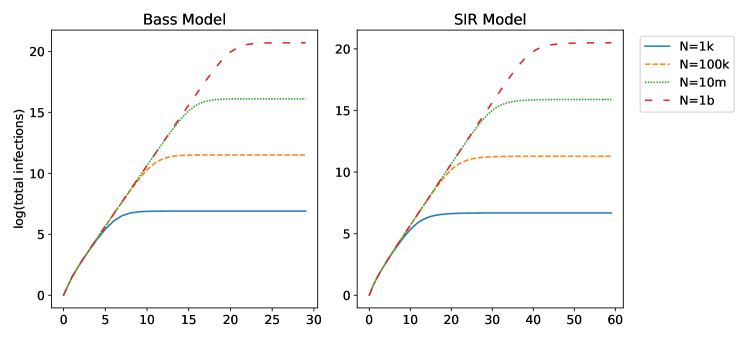
Figure 1: Log of cumulative infections for the deterministic Bass and SIR model with varying $N$. The left figure corresponds Bass models with $\beta=1,p=1/N$. The right figure corresponds to SIR models with $\beta=1,\gamma=0.5$.

The general statement of Theorem 3.3 is a finite-sample result that holds for any initial conditions (see Appendix A.5), which is a direct consequence of applying the Cramer-Rao bound to the following theorem that characterizes the Fisher information of $O_{m}$ relative to $N$.

Theorem 3.4.

Under 3.1 or 3.2, if $m=o(N)$, then the Fisher information of $O_{m}$ relative to $N$ is

(5) $$\mathcal{J}_{O_{m}}(N)=\Theta\left(\frac{m^{3}}{N^{4}}\right).$$

The proof of Theorem 3.4 can be found in Section 4, which involves a non-trivial analysis of the Fisher information of a complex SIR/Bass stochastic process. It is notable that the result above provides a precise rate for the Fisher information as opposed to simply an upper bound. This further allows us to conclude that the relative error rate in Theorem 3.3 is precisely the rate achieved by an efficient unbiased estimator for $N$.

The next section, Section 3.1, analyzes how long it takes to reach $N^{2/3}$ observations. We show that in many parameter regimes, the time it takes to reach $N^{2/3}$ observations is a constant portion (e.g., two thirds) of the time it takes to reach the peak infection rate of the process. In Section 3.2, we analyze the relative error for the other parameters of the model, and we show that these other parameters are much easier to learn than $N$. In Section 3.3, we extend Theorem 3.3 to provide lower bounds for biased estimators.

3.1 Time to Learn

Theorem 3.3 implies that at least $N^{2/3}$ observations are needed before we can learn $N$. Here we characterize how long the diffusion model takes to reach this point relative to the time it takes to reach the point when the rate of new infections is at its peak. In both settings, the peak corresponds to a time in which a constant fraction of the population has been infected.

3.1.1 Bass Model.

One way to characterize the time at which the rate of new adopters in the Bass model peaks is to identify the first epoch at which the expected time until the next adoption increases. That is, defining

$$k^{*}=\inf\{k:\mathbb{E}[T_{k}]\geq\mathbb{E}[T_{k-1}]\ \},$$

$t_{k^{*}}$ corresponds to the (random) time at which this peak in the rate of new adoptions occurs. We denote by $t_{k^{\rm CR}}$ (where $k^{\rm CR}\triangleq\lceil N^{2/3}\rceil$) the earlier time at which we have sufficiently many observations to estimate $N$ accurately per Theorem 3.3. The following result characterizes the ratio ${\mathbb{E}[t_{k^{\rm CR}}]}/{\mathbb{E}[t_{k^{*}}]}$ as $N\rightarrow\infty$:

Proposition 3.5.

Suppose $\gamma=0,I_{0}=1,\frac{p}{\beta}<c$ for some constant $c<1$. Suppose $\frac{p}{\beta}=\Theta(\frac{1}{N^{\alpha}})$ for $\alpha\geq 0$.

$$\lim_{N\rightarrow\infty}\frac{\mathbb{E}[t_{k^{\rm CR}}]}{\mathbb{E}[t_{k^{*}}]}=\begin{cases}0&\alpha\leq\frac{1}{3}\\ \frac{\alpha-\frac{1}{3}}{\alpha}&\frac{1}{3}<\alpha<1\\ \frac{2}{3}&\alpha\geq 1.\end{cases}$$

We see that the fraction of time until peak by which we can hope to learn the Bass model, ${\mathbb{E}[t_{k^{\rm CR}}]}/{\mathbb{E}[t_{k^{*}}]}$, depends on $p/\beta$. This latter quantity provides a measure of the relative contribution of innovators and imitators to the instantaneous rate of overall adoption.

When this quantity is small ($\alpha\geq 1$), we need to wait at least two-thirds of the way until peak to collect enough samples to learn $N$. An interpretation of the regime of $\alpha=1$ is the following. If we treat $\beta$ as a constant, then $p=\Theta(1/N)$. Since the growth of innovators is approximately $pN$ at the start of the process, this regime implies that the number of innovators in the early stages is a constant, which does not depend on $N$. Since $N$ is unknown in the early stages, $\alpha=1$ represents the regime where the rate of innovators at the start of the process does not depend on the (unknown) eventual popularity of the product. There are also many empirical works that estimate the Bass model parameters for consumer products (e.g., air conditioners, TVs, etc.), which establish that adoption is mainly driven by imitation rather than innovation (e.g., Sultan et al. (1990), Mahajan et al. (1995), Lee et al. (2014)).

3.1.2 SIR Model.

For the SIR model, characterizing the random time in which the process hits either the peak infection rate or $N^{2/3}$ observations appears to be a difficult task. Therefore, we analyze the analogs of $t_{k^{\rm CR}}$ and $t_{k^{*}}$ in the deterministic model (1). Specifically, let $t^{d}_{\rm CR}=\inf\left\{t:c(t)\geq N^{2/3}\right\}$ and $t^{d}_{*}=\inf\left\{t:{d^{2}s}/{dt^{2}}>0\right\}$ for the process defined by (1).

Proposition 3.6.

Suppose $p=0$ and $\beta,\gamma$ are fixed. If $c(0)=O(\log(N))$,

$$\liminf_{N\rightarrow\infty}\frac{t^{d}_{\rm CR}}{t^{d}_{*}}\geq\frac{2}{3}.$$

This suggests that the sampling requirements made precise by Theorem 3.3 can only be met at such time where we are close to reaching the peak infection rate. Unlike the Bass model, this ratio is not specific to a parameter regime for the model.

We note that the results of Proposition 3.5 and Proposition 3.6 require $N\to\infty$. While the specific value of ‘two-thirds’ depends on the limit $N\to\infty$, we interpret the significance of this result to be that the time to learning $N$ is a constant fraction of the time to peak (i.e. it is ‘late’), rather than focusing on the precise two-thirds value. In Section 5, we validate this observation on a real-world dataset by demonstrating that the time taken to acquire $N^{2/3}$ observations aligns with the late stages of the diffusion process.

3.2 Estimating Other Parameters

We now turn our attention to learning the other parameters of the model. The high-level message here is that parameters other than the population $N$ are in general easier to learn, and this is best understood through Table 1. Specifically, the second row in that table shows the number of observations needed for a relative error less than one. Our earlier analysis provides lower bounds on this quantity for the estimation of $N$. Here we construct explicit estimators for the remaining parameters yielding upper bounds on the number of observations required to learn those parameters with a relative error less than one.

We immediately see that for the SIR model, we can accomplish this task with a number of observations that does not scale with the population size parameter. In the case of the Bass model the story is more nuanced: it is always easier to learn the coefficient of imitation, $\beta$. On the other hand when the rate of innovation is very low, learning $a:=pN$ is hard, but also not relevant to tasks related to forecasting $N$. We next present formal results that support the quantities in Table 1.

Table 1: Summary of parameter estimation results for the Bass and SIR models. The first row shows the relative error of estimating each parameter with $m$ observations. The second row shows $\operatorname*{\mathrm{argmin}}_{m}\{\mathrm{RelError}(\hat{\theta}_{m},\theta)\leq 1\}$, the number of observations needed so that the relative error is less than 1. For the Bass model, $a=pN$, and $a=\Theta(N^{1-\alpha})$ for $\alpha\geq 0$.

		Bass		SIR
	$N$*	$\beta$	$a$**	$\beta$	$\gamma$
$\mathrm{RelError}(\hat{\theta}_{m},\theta)$	$\Omega\left(\frac{N^{2}}{m^{3}}\right)$	$\tilde{O}\left(\frac{1}{m}+\frac{N^{2(1-\alpha)}}{m^{3}}\right)$	$\tilde{O}\left(\frac{1}{m}+\frac{1}{N^{(1-\alpha)}}\right)$	${O}\left(\frac{\log m}{m}\right)$	${O}\left(\frac{\log m}{m}\right)$
# observations needed	$\Omega\left(N^{2/3}\right)$	$\tilde{O}\left(\max\{1,N^{\frac{2}{3}(1-\alpha)}\}\right)$	$\tilde{O}\left(1\right)$	$O\left(1\right)$	$O\left(1\right)$

*The column for $N$ represents the expected relative error, whereas the other parameters are high-probability results.
**We note that the results for the parameter $a$ hold only for $\alpha<1$.

3.2.1 Bass Model.

For the Bass model, we construct estimators for the parameters $\beta$ and $a:=pN$ (the explicit construction is given in Appendix B):

Theorem 3.7.

Suppose $\gamma=0$ and $I_{0}=1$. Let $a=pN.$ Suppose $m\leq N^{2/3}\log^{1/3}(N)$. We construct estimators $\hat{a}_{m},\hat{\beta}_{m}$ based on the observations $O_{m}$ such that with probability $1-O(\frac{1}{N})$,

$$\mathrm{RelError}(\hat{\beta}_{m},\beta)=O\left(\frac{\log N}{m}+\frac{a^{2}}{\beta^{2}}\frac{\log N}{m^{3}}\right),$$

$$\mathrm{RelError}(\hat{a}_{m},a)=O\left(\frac{\log N}{m}+\frac{\beta}{a}\log N\right).$$

The above result demonstrates that learning the coefficient of imitation, $\beta$, is always easier than estimating $N$. This is also the case for $a$ when $p/\beta=\omega(1/N)$; when $p/\beta=O(1/N)$, the number of innovators who adopt is negligible compared to the number of imitators and it is not possible to estimate $a$.

3.2.2 SIR Model.

For the SIR model we construct estimators for the parameters $\beta$ and $\gamma$ (the explicit construction is given in Section C.1):

Theorem 3.8.

Suppose $p=0$ and $\beta>\gamma$. Let $C_{0},m,N$ satisfy $m(m+C_{0})\leq N$, and $\frac{\beta}{\beta+\gamma}\frac{N-m-C_{0}}{N}>\frac{1}{2}(\frac{\beta}{\beta+\gamma}+\frac{1}{2})$. Then, we can construct estimators $\hat{\beta}_{m}$ and $\hat{\gamma}_{m}$, both functions of $O_{m}$, such that with probability $1-\frac{8}{m}-B_{1}e^{-B_{2}I_{0}}$,

$$\mathrm{RelError}(\hat{\beta}_{m},\beta) \leq M_{1}\left(\frac{\log m}{m}\right),$$

$$\mathrm{RelError}(\hat{\gamma}_{m},\gamma) \leq M_{2}\left(\frac{\beta^{2}}{\gamma^{2}}\frac{\log m}{m}\right),$$

where $M_{1},M_{2}>0$ are absolute constants and $B_{1},B_{2}>0$ depends only on $\beta$ and $\gamma$.

When $\beta$ and $\gamma$ do not scale with the size of the system $N$ (which is the case for epidemics), this result shows that the relative error for both estimators is $O\left({\log m}/{m}\right)$, i.e. independent of $N$. Consequently, to achieve any desired level of accuracy, we simply need the number of observations $m$ to exceed a constant that is independent of the size of the system. This is in stark contrast to Theorem 3.3, in which $m$ needs to scale at least as $\omega(N^{2/3})$ in order to learn $N$.

3.3 Extension to Biased Estimators

Although we focus on unbiased estimators of $N$ in this work, a lower bound for biased estimators of $N$ can also be easily obtained via the generalized Cramer-Rao bound (Cramér et al. 1946), which bounds the variance of biased estimators with given bias and Fisher information. Using the Fisher information from Theorem 3.4, the generalized Cramer-Rao bound implies the following result.

Proposition 3.9.

Under 3.1 or 3.2, if $\hat{N}_{m}$ is a biased estimator of $N$, with bias $b(N)=\mathbb{E}[\hat{N}_{m}]-N$, based on the observations $O_{m}$,

(6) $$\mathbb{E}[\mathrm{RelError}(\hat{N}_{m},N)]=\Omega\left(\frac{N^{2}(1+b^{\prime}(N))^{2}}{m^{3}}+\frac{b(N)^{2}}{N^{2}}\right).$$

When $|1+b^{\prime}(N)|<1$, this bound may be less than the unbiased Cramer-Rao bound in Theorem 3.3. The result can be used to guide the design of estimators for balancing the bias and variance (Eldar 2008).

3.4 Decision Problem

In this section, we formalize a generic decision problem in the context of an epidemic. The decision is whether to impose a ‘drastic intervention’ that is associated with a cost, but will immediately stop all further infections. We establish a lower bound on the regret that any policy will incur for this decision problem.

We assume that there is a cost, $f_{1}>0$, for every infected individual. A drastic intervention will immediately stop any further new infections, but the intervention will incur a fixed cost of $f_{0}>0$. Then, a drastic intervention implemented at step $m$ incurs a cost of $f_{0}+f_{1}C_{m}$, recalling that $C_{m}$ represents the cumulative number of infected individuals up to step $m$. On the other hand, if no intervention is implemented, the cost is solely from the infections, which is $f_{1}C_{\infty}$, where $C_{\infty}$ represents the total number of accumulated infections at the end of the epidemic. We study policies that decide when, if ever, to deploy this drastic intervention.

A problem instance is defined as $\mathcal{M}=(f_{0},f_{1},\beta,\gamma,N)$. We define the optimal cost as ${\rm{cost}}^{*}(\mathcal{M})=\min\{f_{0}+f_{1}C_{0},f_{1}C_{\infty}\}$, which is the cost of the optimal policy that has knowledge of the entire problem instance, $\mathcal{M}$. We consider policies that have knowledge of all parameters except $N$. The policy has access to all of the observations of the diffusion process, and the policy faces a stopping problem regarding whether and when to employ the drastic intervention. The regret of a policy $\pi$ is:

(7) $${\rm{regret}}^{\pi}(\mathcal{M}):=\mathrm{E}[{\rm{cost}}^{\pi}(\mathcal{M})]-{\rm{cost}}^{*}(\mathcal{M}).$$

We prove the following lower bound on the regret.

Proposition 3.10.

There exists a set of problem instances $\mathcal{S}_{N}$ that are parameterized by $N$, for any policy $\pi$,

$$\sup_{\mathcal{M}\in\mathcal{S}_{N}}{\rm{regret}}^{\pi}(\mathcal{M})=\Omega(N^{2/3}).$$

That is, the lower bound on the regret for any policy $\pi$ is $\Omega(N^{2/3}).$

The proof of Proposition 3.10 relies on constructing two instances where the optimal decision is different, but it is difficult to distinguish between these two instances due to the uncertainty in the estimation of $N$. The full proof can be found in Appendix D.5. This result shows that the hardness in estimating $N$ translates directly to the difficulty of a generic decision problem on implementing an intervention.

3.5 Addressing Under-reporting through Seroprevalence Testing

The results so far have demonstrated that the estimation of the parameter $N$ is the bottleneck for forecasting using infection data. In the epidemic setting, and for COVID-19 in particular, one of the main source of uncertainty in $N$ came from under-reporting (Li et al. 2020, Lau et al. 2021, Pullano et al. 2021). To overcome this challenge, one can potentially use other data sources in order to improve the estimation of $N$. For instance, for COVID-19, surveillance tests were often conducted to estimate the prevalence of infections without under-reporting bias (Havers et al. 2020, Bendavid et al. 2021). In this section, we study the value of utilizing such a dataset. Specifically, we assume that a random sample of $K$ people are tested for the infection after $m$ observations of the SIR process. We compute the value of this information via the Fisher information and the Cramer-Rao bound, analogous to our main result of Theorem 3.3.

After $m$ observations of the SIR process, we assume that $K$ people are chosen at random to be tested for infection. Then, the infection rate for a randomly chosen person is:

$$\kappa_{m}=\frac{E[C_{m}]}{N},$$

which is the ratio between the expected cumulative number of observed infections and the (effective) population. Letting $X_{k}\sim\mathrm{Ber}(\kappa_{m})$ be independent Bernoulli random variables that represent the infection outcome of the $k$-th chosen patient, the observation set from the test is:

$$\tilde{O}_{m}=(X_{1},X_{2},\dotsc,X_{K}).$$

Considering this additional information, we establish the following result.

Proposition 3.11.

Under Assumption 2, if $m=o(N)$, then the Fisher information of $O_{m}\cup\tilde{O}_{m}$ relative to $N$ is:

$$J_{{O_{m}\cup\tilde{O}_{m}}}(N)=\Theta\left(\frac{m^{3}}{N^{4}}\right)+\Theta\left(\frac{Km}{N^{3}}\right)$$

where $\Theta\left(\frac{Km}{N^{3}}\right)$ quantifies the exact additional Fisher information provided by $\tilde{O}_{m}$.

The proof can be found in Appendix D.6. Using this, we apply the Cramer-Rao bound for estimating $N$ based on $\tilde{O}_{m}$.

Corollary 3.12.

For any unbiased estimator $\hat{N}_{m}$ of $N$ based on the observations $\tilde{O}_{m}$,

$$\mathbb{E}[\text{RelError}(\hat{N}_{m},N)]=\Omega\left(\frac{N}{Km}\right).$$

Corollary 3.12 provides a lower bound for estimating $N$ using a seroprevalence study, and a naive MLE estimator can be used to achieve the lower bound. In order for $\mathbb{E}[\text{RelError}(\hat{N}_{m},N)]=o(1)$, it is necessary to ensure that $Km=\omega(N)$. This clearly delineates the trade-off in the size of the campaign, $K$, versus the timing of the campaign, $m$. For example, if $m=\Theta(N^{1/3})$ we require $K=\omega(N^{2/3})$. Therefore, with a sufficiently large seroprevalence test, we have the potential to surpass the lower bound barrier of two-thirds in the early stages of the epidemic.

4 Proof of Theorem 3.4

Recall that $O_{m}=(I_{0},R_{0},T_{1},C_{1},\dots,T_{m},C_{m})$. We will take advantage of conditional independence to decompose the Fisher information $\mathcal{J}_{O_{m}}(N)$ into smaller pieces. We first define the conditional Fisher information and state some known properties (Zegers 2015).

Definition 4.1.

Suppose $X,Y$ are random variables defined on the same probability space whose distributions depend on a parameter $\theta$. Let $g_{X|Y}(x,y,\theta)=\frac{\partial}{\partial\theta}\log f_{X|Y;\theta}(x|y)^{2}$ be the square of the score of the conditional distribution of $X$ given $Y=y$ with parameter $\theta$ evaluated at $x$. Then, the conditional Fisher information is defined as $\mathcal{J}_{X|Y}(\theta)=\mathbb{E}_{X,Y}\left[g_{X|Y}(X,Y,\theta)\right]$.

Property 4.2.

$\mathcal{J}_{X_{1},\dots,X_{n}}(\theta)=\mathcal{J}_{X_{1}}(\theta)+\sum_{i=2}^{n}\mathcal{J}_{X_{i}|X_{1},\dots,X_{i-1}}(\theta)$.

Property 4.3.

If $X$ is independent of $Z$ conditioned on $Y$, $\mathcal{J}_{X|Y,Z}(\theta)=\mathcal{J}_{X|Y}(\theta)$.

Property 4.4.

If $X$ is deterministic given $Y=y$, $g_{X|Y}(X,y,\theta)=0$.

Property 4.5.

If $\theta(\eta)$ is a continuously differentiable function of $\eta$, $\mathcal{J}_{X}(\eta)=\mathcal{J}_{X}(\theta(\eta))(\frac{d\theta}{d\eta})^{2}$.

Since $I_{0}$ and $R_{0}$ are known and not random, the Fisher information of $O_{m}$ is equal to the Fisher information of $(T_{1},C_{1},T_{2},C_{2},\dots,T_{m},C_{m})$. Then, Property 4.2 implies

(8) $$\mathcal{J}_{O_{m}}(N) =\mathcal{J}_{T_{1}}(N)+\mathcal{J}_{C_{1}|T_{1}}(N)+\mathcal{J}_{T_{2}|T_{1},C_{1}}(N)+\mathcal{J}_{C_{2}|T_{1},C_{1},T_{2}}(N)+\dots+\mathcal{J}_{C_{M}|T_{1},C_{1},\dots,T_{m}}(N).$$

Bass Model: The above expression simplifies greatly for the Bass model since every event corresponds to a new infection. That is, we know $C_{k}=I_{k}=I_{0}+k$ and $S_{k}=N-k-I_{0}$ deterministically. Therefore, Property 4.4 implies that $\mathcal{J}_{C_{k}|\cdot}(N)=0$ for all $k$. Moreoever, since $T_{k}\sim\exp(\beta\frac{S_{k-1}}{N}I_{k-1}+\frac{a}{N}S_{k-1})$ is independent of $T_{1},C_{1},\dots,C_{k-1}$, $\mathcal{J}_{T_{k}|T_{1},C_{1},\dots,C_{k-1}}(N)=\mathcal{J}_{T_{k}}(N)$. This yields

(9) $$\mathcal{J}_{O_{m}}(N) =\sum_{k=1}^{m}\mathcal{J}_{T_{k}}(N).$$

By letting $\lambda_{k}(N)=\left(\frac{\beta}{N}(k+I_{0})+\frac{a}{N}\right)(N-k-I_{0})$, since $T_{k}\sim\exp(\lambda_{k}(N))$, Property 4.5 says that $\mathcal{J}_{T_{k}}(N)=\mathcal{J}_{T_{k}}(\lambda_{k})\left(\frac{d\lambda_{k}}{dN}\right)^{2}$. Using that the Fisher Information of an exponential distribution with parameter $\lambda$ is $\frac{1}{\lambda^{2}}$, a few lines of algebra yields $\mathcal{J}_{T_{k}}(N)=\frac{(k+I_{0})^{2}}{N^{2}(N-k-I_{0})^{2}}$. Plugging back into (9), we get

(10) $$\mathcal{J}_{O_{m}}(N)=\frac{1}{N^{2}}\sum_{k=1}^{m}\frac{(k+I_{0})^{2}}{(N-k-I_{0})^{2}}.$$

Using $I_{0}=1$ and $m=o(N)$ from 3.1, we get the desired result $\mathcal{J}_{O_{m}}(N)=\Theta\left(\frac{m^{3}}{N^{4}}\right)$.

SIR Model: The analysis for the SIR model is more complicated since $C_{k}$ is not deterministic and the distribution of $T_{k}$ depends on $C_{k-1}$. Moreover, there is a non-zero probability that the process has terminated before the $k$’th jump for any $k$. Define the indicator variable $E_{k}=\mathds{1}\{\tau>k\}$ on the event that the SIR process has not terminated after $k$ jumps. The following lemma states that both $E_{k}$ and $I_{k}$ can be determined from $C_{k}$, $I_{0}$, and $R_{0}$, which will allow us to decouple variables in $O_{m}$ in the analysis of the Fisher information. The result follows from the definitions of $\tau$, $E_{k}$, and $C_{k}$; the details can be found in the Appendix.

Lemma 4.6.

Define $r_{k}\triangleq\frac{I_{0}+k+2R_{0}}{2}$ for all $k\geq 0$. For all $k$, $E_{k}=\mathds{1}\{C_{k}>r_{k}\}$. Moreover, when $E_{k}=1$, $I_{k}=2C_{k}-k-I_{0}-2R_{0}>0$.

The next lemma writes an exact expression for $\mathcal{J}_{O_{m}}(N)$, analogous of (10) for the Bass model:

Lemma 4.7.

The Fisher information of the observations $O_{m}$ with respect to the parameter $N$ is

(11) $$\mathcal{J}_{O_{m}}(N) =\sum_{k=1}^{m}\Pr(E_{k-1}=1)\mathbb{E}\left[\frac{C_{k-1}^{2}}{N^{2}(N-C_{k-1})(N-C_{k-1}+\frac{\gamma}{\beta}N)}\;\bigg{|}\;E_{k-1}=1\right].$$

Proof.

We start from (8). Note that for any $k$, $C_{k}$ and $T_{k}$ only depend on $C_{k-1}$. Indeed, since $C_{k-1}$ determines $E_{k-1}$, if $E_{k-1}=0$ (the stopping time has passed), we have $C_{k}=C_{k-1}$ and $T_{k}=\infty$. When $E_{k-1}=1$, the distributions of $C_{k}$ and $T_{k}$ are given in (2)-(3). Since $\beta,\gamma,I_{0},R_{0}$ are known, $S_{k-1}=P-C_{k-1}$, and $I_{k-1}$ can be determined from $C_{k-1}$ (Lemma 4.6), the distributions of $C_{k}$ and $T_{k}$ are determined by $C_{k-1}$. Therefore, we use Property 4.3 to simplify (8) to

$$\mathcal{J}_{O_{m}}(N) =\sum_{k=1}^{m}(\mathcal{J}_{C_{k}|C_{k-1}}(N)+\mathcal{J}_{T_{k}|C_{k-1}}(N)),$$

where we used $\mathcal{J}_{T_{1}}(N)=\mathcal{J}_{T_{1}|C_{0}}(N)$, $\mathcal{J}_{C_{1}}(N)=\mathcal{J}_{C_{1}|C_{0}}(N)$. Moreover, when $E_{k-1}=0$, $C_{k}$ and $T_{k}$ are deterministic conditioned on $C_{k-1}$, which implies the score in this case is 0 (Property 4.4). Therefore, we can condition on $E_{k-1}=1$ to write

$$\mathcal{J}_{O_{m}}(N) =\sum_{k=1}^{m}\mathbb{E}[g_{C_{k}|C_{k-1}}(C_{k},C_{k-1},N)+g_{T_{k}|C_{k-1}}(T_{k},C_{k-1},N)|E_{k-1}=1]\Pr(E_{k-1}=1).$$

The last step is to evaluate $g_{C_{k}|C_{k-1}}(C_{k},C_{k-1},N)$ and $g_{T_{k}|C_{k-1}}(T_{k},C_{k-1},N)$. When $E_{k-1}=1$, the distributions of $C_{k}$ and $T_{k}$ conditioned on $C_{k-1}$ have a simple form provided in (2)-(3). Property 4.5 allows for straight-forward calculations, resulting in (11). See Section A.3 for details of this last step. $\square$

What remains is to upper and lower bound (11). The upper bound $\mathcal{J}_{O_{m}}(N)=O\left(\frac{m^{3}}{N^{4}}\right)$ follows from upper bounding $\Pr(E_{k-1})$ by 1 and the fact that $C_{k-1}$ is small relative to $N$ (details of this step are in Section A.4). As for the lower bound, we first show a lower bound for $\Pr(E_{k-1}=1)$ using the following lemma:

Lemma 4.8.

Let $p=\frac{1}{2}\left(\frac{\beta}{\beta+\gamma}+\frac{1}{2}\right)>\frac{1}{2}$. There exists a constant $D$ that only depends on $\beta$ and $\gamma$ such that if $\frac{\beta(P-m-C_{0})}{\beta(P-m-C_{0})+P\gamma}>p$ and $I_{0}\geq D$, then $\Pr(E_{m}=1)\geq\frac{1}{2}$.

This result relies on an interesting stochastic dominance argument and can be found in the appendix. Then, similarly to the upper bound, $\mathcal{J}_{O_{m}}(N)=\Omega\left(\frac{m^{3}}{N^{4}}\right)$ follows from using $\Pr(E_{m}=1)\geq\frac{1}{2}$ and the fact that $C_{k}\geq\frac{k+I_{0}+2R_{0}}{2}$ when $E_{k}=1$ (Lemma 4.6).

5 Numerical Results

We run experiments on real-world datasets for both the Bass and SIR models to demonstrate how the theoretical results from Section 3 manifest in practice. We describe three sets of empirical results:

• Section 5.2 mirrors the theory in this paper and makes two points: First, the relative error one sees in real-world datasets on quantities of interest as a function of the number of observations closely hews to that predicted by our results. Second, the time at which predictions of key quantities ‘turn accurate’ is late in the diffusion and again matches our theory.

• In Section 5.3, we conduct a set of semi-synthetic experiments on a variant of the SIR model that captures heterogeneously mixing subpopulations. Since the SIR model assumes that the population mixes uniformly, a practical use of the SIR model needs to be at the right level of granularity. We show that even when we divide the population into smaller subpopulations with different mixing rates, we observe the same phenomenon regarding the estimation of $N$ — the accuracy sharply increases after $N^{2/3}$ observations.

• In Section 5.4, we describe an approach for COVID-19 forecasting of US counties that leverages an informative bias on $N$ to work around the limits of learning. We consider a realistic variant of the SIR model that accounts for non-stationarities and rich county-level covariates, and we employ a heuristic for estimating the parameters that was directly inspired by our main theoretical results. Specifically, this estimation method leverages the plurality of US counties, as well as the heterogeneity in the timing of COVID-19 infections across these counties. We show that the insight of our estimation results can guide the development of forecasting methods which significantly improved the forecasting power, compared to a naive estimation method.

5.1 A Discrete-Time Diffusion Model

First, we describe the standard Euler-Maruyama discretization of our stochastic diffusion model; this discretization better aligns with aggregated (as opposed to event level) data. Real-world data is often stored as arrival counts $\Delta C_{i}[t]$ over a set of discrete time periods $t\in[T]$ and problem instances $i\in\mathcal{I}$. We model these counts as the following Poisson process, obtained by approximately discretizing the exponential arrival process (3). Precisely, we divide the time horizon into $T$ epochs of length $1$, where at each epoch $t\in[T]$ we observe random variables:

(12) $$\Delta C_{i}[t] \sim\mathrm{Poisson}(\lambda_{i,t}(a_{i},\beta_{i},N_{i}))$$

$$\Delta R_{i}[t] \sim\mathrm{Poisson}(\gamma I_{i}[t-1])$$

where $\lambda_{i,t}(a,\beta,N)=(a+\beta I[t-1])\frac{S[t-1]}{N}$, and $\Delta C_{i}[t]$ and $\Delta R_{i}[t]$ are independent. Essentially, we evaluate the arrival rate of (3) at the beginning of each epoch, and assume that it remains constant over the course of the epoch. This arrival process is then split into $\Delta C_{i}[t]$ and $\Delta R_{i}[t]$ according to the probabilities in (2). The state space then evolves according to:

(13) $$S_{i}[t] =S_{i}[t-1]-\Delta C_{i}[t]$$

$$I_{i}[t] =I_{i}[t-1]+\Delta C_{i}[t]-\Delta R_{i}[t]$$

$$R_{i}[t] =R_{i}[t-1]+\Delta R_{i}[t]$$

For the datasets we study, $\gamma$ is known a priori, (i.e. from clinical data for the ILINet flu datasets; for the Bass model $\gamma=0$). We then obtain maximum likelihood estimates $\hat{a}_{i}[t],\hat{\beta}_{i}[t],\hat{N}_{i}[t]$ for the remaining parameters by solving the problem:

(14) $$\max_{\begin{subarray}{c}a,\beta,N\in[0,N_{\max}]\end{subarray}}\quad\sum_{\tau=1}^{t}\log p(\Delta C_{i}[\tau];\lambda_{i,\tau}(a,\beta,N))$$

where $p(x;\lambda)=\frac{\lambda^{x}\exp(-\lambda)}{x!}$ denotes the Poisson PMF with rate parameter $\lambda$, and $N_{\max}$ is an upper bound on $N$ known a priori. This reflects that loose upper bounds on $N$ (e.g., the entire population of a geographic region, for epidemic forecasting) are typically known in real-world problems.

5.2 MLE Performance on Benchmark Datasets

In this section, we fit the Bass and SIR models to real-world datasets and compare the empirical results to the theoretical results from Section 3.

Datasets.

We fit the Bass model to a dataset of Amazon product reviews from Ni et al. (2019), which we take as a proxy for product adoption. Here each instance $i$ is a product, $t$ indexes weeks since the product’s first review, and $I_{i}[t]$ represents cumulative number of reviews for product $i$. For the SIR model, we use the CDC’s ILINet database of patient visits for flu-like illnesses. Here, each instance $i$ is a geographic region, $t$ indexes weeks, and $I_{i}[t]$ represents infected patients. See Appendix E for further details on these datasets.

Comparing actual error to error predicted from theory.

Here we fit diffusion models to products from the Amazon data, as well as individual seasons from the ILINet data, while varying the number of observations used to fit the model. We compare the observed relative error in predicting the effective population size $N$ in each to the error predicted by Theorem 3.3. We find that Theorem 3.3 provides a valuable lower bound despite potential model mis-specification, aggregated data, and the fact that we jointly estimate the $a,\beta$ and $N$ parameters.

Specifically, let $T_{i}$ be the time index of the last observation we have for product $i$. We take $\hat{N}_{i}[T_{i}]$ to be the ground truth parameter for product $i$. Figure 2 is a scatter plot of the mean (over instances $i$ and times $t$) observed relative error $\mathrm{RelError}(\hat{N}_{i}[t],\hat{N}_{i}[T_{i}])$ against the Cramer-Rao lower bound of Theorem 3.3, $M{\hat{N}_{i}[T_{i}]^{2}}/{C_{i}[t]^{3}}$, where $M$ is a lower bound on the constant suppressed in the statement of Theorem 3.3. In addition to providing a lower bound, we find that the slope of the relationship is close to one in both datasets as the error grows small. It is worth re-emphasizing that this is the case despite the fact that the data here is not synthetic, so the Bass and SIR models are almost certainly not a perfect fit to the data.

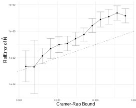
(a) Bass model fit on Amazon product reviews.

(b) SIR model fit on ILINet patient visits.

Figure 2: Each figure shows the mean of $\mathrm{RelError}(\hat{N}_{i}[t],\hat{N}_{i}[T_{i}])$ over instances $i\in\mathcal{I}$ and times $t\in[T]$ (error bars show 95% CIs), vs. the Cramer-Rao bound $\frac{M\hat{N}_{i}[T_{i}]^{2}}{C_{i}[t]^{3}}$, where $M$ is a lower bound on the constant suppressed in the statement of Theorem 3.3. We also show the $y=x$ line (dashed gray) for comparison. As predicted, the Cramer-Rao bound provides a lower bound on $\mathrm{RelError}(\hat{N}_{i}[t],\hat{N}_{i}[T_{i}])$, and the slope of this relationship is close to 1 as the error grows small.

Time to accuracy of peak predictions.

As discussed earlier, predicting the peak of the infection process is a key task in the SIR model (as is predicting the peak in new adoptions in the Bass model). Here we show, through the ILINet data, that the time at which our prediction of the peak number of infections in an epidemic ‘turns accurate’ is close to the peak and matches what our theory suggests. Specifically, let $I^{*}_{i}=\max_{t\in[T_{i}]}I_{i}[t]$ be the maximal number of infections. Given estimates $\hat{\beta},\hat{N}$ of the diffusion parameters, we define a point estimate for the peak number of infections

$$\hat{I}^{*}_{i}(\hat{\beta},\hat{N})=\mathbb{E}\left[\max_{\tau\in[T_{i}]}I_{i}[\tau]\,\big{|}\,\hat{\beta},\hat{N}\right].$$

The solid line in Figure 3 depicts errors for the estimator $I^{*}_{i}(\hat{\beta}_{i}[t],\hat{N}_{i}[t])$, where $\hat{\beta}_{i}[t],\hat{N}_{i}[t]$ are the MLE using data up to time $t$. At 66% of time to peak, around 50% of instances predict peak infections with $>50\%$ error. By the time the peak actually occurs, around 40% of instances still suffer prediction error in this range. Errors then drop off sharply after this point.

For comparison, let $\tilde{\beta}_{i}[t]$ be the solution to the MLE problem (14) fixing $N=\hat{N}_{i}[T_{i}]$; that is, the MLE for $\beta$ if we knew the ground-truth value of $N$ a priori. The dashed line in Figure 3 shows errors for the peak estimate $I^{*}(\tilde{\beta}_{i}[t],\hat{N}_{i}[T_{i}])$. Errors for this estimator drop off much more quickly, with almost $90\%$ of instances achieving $<50\%$ error by $66\%$ of time to peak. This bears out the predictions of Theorem 3.8 that once $N$ is known, the remaining parameters of the SIR process are easy to estimate.

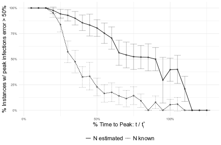
Figure 3: % of instances with with relative prediction error $\left\lvert\hat{I}^{*}_{i}(\hat{\beta},\hat{N})-I^{*}_{i}\right\rvert/I^{*}_{i}>0.5$, vs. % of time to peak on the ILINet dataset. For ‘N estimated’, we evaluate the MLE at time $t$ $\hat{I}^{*}(\hat{\beta}_{i}[t],\hat{N}_{i}[t])$. Errors for this estimator remain unreasonably large until around the peak occurs – after which it drops dramatically. For ‘$N$ known’, we evaluate the estimator $\hat{I}^{*}(\tilde{\beta}_{i}[t],\hat{N}_{i}[T_{i}])$; that is, we assume $N$ known and estimate $\beta$ via MLE. Here, most instances estimate the peak accurately after 66% of time to peak, reflecting the ease of estimating $\beta$ given $N$.

Time to reach a lower bound of $\mathrm{RelError}(\hat{N})=o(1)$.

Finally, to understand the implications of our theory at a practical scale, we consider how long it takes to achieve a sample size large enough for Theorem 3.3 to admit an error of $\mathrm{RelError}(\hat{N})=o(1)$. In other words, how long (in real time) it takes to achieve roughly $N^{2/3}$ samples. We consider here the Amazon dataset under the Bass model. We first estimate $N$ for each product via MLE on all observations; use this estimated $N$ to determine the minimum required number of observations; then determine from the dataset how long it takes to reach that many observations. Figure 4 shows that this time is extremely long in practice: greater than 6 months for about 75% of products; and greater than one year for 50% of products. Notably, this is roughly the same time to sell $N/4$ units — a constant fraction of all the units that will ever be sold.

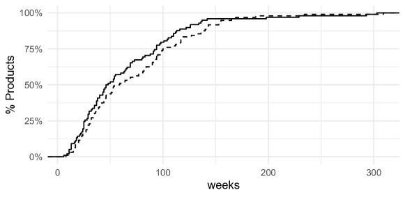
Figure 4: The solid line shows the cumulative distribution of the time needed to achieve a RelError lower bound of $o(1)$ (as given by Theorem 3.3), for products in the Amazon dataset. This is greater than 6 months for about 75% of products; and greater than one year for 50% of products. The dashed line shows the cumulative distribution of the time need to sell $N/4$ products; these distributions are comparable.

5.3 Heterogeneous Mixing Subpopulations

We now consider a variant of the SIR model in which the population is partitioned into groups based on their mixing rates. The goal is to determine whether our main results hold under a more complex SIR variant that better captures real-world population dynamics.

We follow Del Valle et al. (2007), which defines subpopulations as age groups $[0,5),[5,10)\ldots[70,\infty)$. They provide mixing rates within and between age groups based on contact data collected in each of 131 countries. The paper also provides populations per age group per country, and an estimate of the ‘clinical fraction’, i.e., the proportion of each age group which will present with clinically significant symptoms.

For each country, we use this data to construct a semi-synthetic instance with realistic subpopulations and mixing conditions. We assume for simplicity that the clinical fraction represents the ‘true’ infected proportion of each subpopulation. Let $N_{i}$ be the total susceptible population in each subpopulation (i.e., population of the subpopulation, times clinical fraction) and let $N=\sum_{i=1}^{n}N_{i}$ be the total susceptible population across subpopulations. We will further simplify by assuming that the mixing rates $B_{ij}$, recovery rates $\gamma_{i}$ and population ratios $N_{i}/N$ are all known; but the decision maker must still estimate the overall scale $N$. We will show empirically that our results continue to hold in this more realistic setting – even though there remains only one parameter to estimate.

The specific compartmental model we use is a stochastic generalization of Del Valle et al. (2013), following a jump process model analogous to that in our existing results. At each jump $k\in\mathbb{N}$, we observe either an infection or recovery in some subpopulation, as well as the time between events $k-1$ and $k$. Let $B\in\mathbb{R}^{n\times n}$ be the matrix of transmission rates between subpopulations, and let $\gamma\in\mathbb{R}^{n}$ be the recovery rate within each subpopulation. Define the infection and recovery rates for subpopulation $i$ after the $k^{\rm th}$ event as follows:

$$\lambda_{ik}^{I} =\sum_{j\in[n]}B_{ij}\frac{S_{ik}I_{jk}}{N_{j}}$$

$$\lambda_{ik}^{R} =\gamma_{i}I_{ik}$$

Then, let $T_{t}$ denote the duration between events $k-1$ and $k$:

$$T_{k+1} \sim{\rm Exp}\left(\sum_{i=1}^{n}(\lambda_{ik}^{I}+\lambda_{ik}^{R})\right)$$

State dynamics are as follows. There are $2n$ mutually exclusive events possible each epoch: Infection in subpopulation $i$, and Recovery in subpopulation $i$, for each $i\in[n]$. On event Infection $i$, we have $S_{i,k+1}=S_{ik}-1$, and $I_{i,k+1}=I_{ik}+1$. All other state dimensions unchanged. On event Recovery $i$, we have $R_{i,k+1}=R_{i,k+1}+1$ and $I_{i,k+1}=I_{ik}-1$. All other state dimensions unchanged. Conditional on history, these have probabilities

$$P(\text{Infection }i) =\lambda_{ik}^{I}/\sum_{i=1}^{N}(\lambda_{ik}^{I}+\lambda_{ik}^{R})$$

$$P(\text{Recovery }i) =\lambda_{ik}^{R}/\sum_{i=1}^{N}(\lambda_{ik}^{I}+\lambda_{ik}^{R})$$

Figure 5 shows the error in estimating $N$ as a function of $m$, the number of events observed, averaged over all 131 countries. Here we see that, precisely as the theory predicts, the relative error in estimating $N$ is significantly larger than 1 until $m>N^{2/3}$. After this point, the error drops precipitously, and precise estimation of $N$ becomes possible. Figure 6 shows results by country for 20 randomly selected countries, demonstrating that this holds not only in aggregate, but also for each individual problem instance.

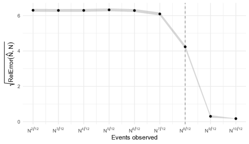
Figure 5: Error in estimating $N$ as a function of $m$, the number of events observed, averaged over all 131 countries. Error bars show standard errors over 50 random seeds.${\rm RelError}(\hat{N},N)$ is significantly above 1 until $m>N^{2/3}$, after which the error drops sharply.

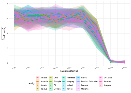
Figure 6: Error in estimating $N$ as a function of $m$, the number of events observed, for 20 randomly chosen countries. Error bars show standard errors over 50 random seeds. In all instances, ${\rm RelError}(\hat{N},N)$ is significantly above 1 until $m>N^{2/3}$, after which the error drops sharply.

5.4 Working Around the Limits to Learning in the COVID-19 Pandemic

One approach to bypass the limits of learning is to rely on an estimator that places an informative prior on the effective population parameter, $N$. Here we briefly describe a heuristic that used this idea, which was used to produce one of the first broadly available county-level forecasts for COVID-19.

As above, we would like to forecast infections for a set of regions $i\in\mathcal{I}$. Recall that the effective population $N_{i}$ for region $i$ is the product of the actual population of the region (which is obviously known) and the fraction of infections that are actually observed (which is not). To arrive at a useful bias for $N_{i}$, we exploit hetereogeneity in the timing of infections in each region and use a ‘two-stage estimation’ method. Specifically, infections start at different times in each region, and we typically have access to some set $Q[t]\subseteq\mathcal{I}$ of regions that have already experienced enough infections to reliably estimate $N_{i}$ for $i\in Q[t]$. At a high level, our strategy will be to identify the set $Q[t]$, estimate $N_{i}$ for $i\in Q[t]$, then extrapolate these estimates (e.g., via matching on region-level covariates) to obtain $N_{i}$ for $i\notin Q[t]$. We describe this methodology briefly in the following section, as well as in detail in Appendix F.

5.4.1 Two-Stage Estimation.

Letting $P_{i}$ be the known population of region $i$, we parameterize the effective population as $N_{i}(\phi,\delta)=\exp(\phi^{\top}Z_{i}+\delta_{i})P_{i}$, where $Z_{i}$ are non-time-varying, region-specific covariates, $P_{i}$ is the population of region $i$, $\phi$ is a vector of fixed effects, and $\delta_{i}\sim\mathcal{N}(0,\sigma^{2}_{\delta})$ are region-specific random effects.

Next, we also incorporate demographic and mobility factors into the model, which influence the reproduction rate. We define $X_{i}[t]$ as a set of time-varying covariates for region $i$, which represent both demographic features of the region as well as dynamic mobility features that represent the amount of movement of people in the county (leveraging anonymized location data). Then, we write $\beta_{i}[t]$ as a mixed effects model incorporating covariates $\beta_{i}[t]=\exp(X_{i}[t]^{\top}\theta)+\epsilon_{i}$, where $\theta$ is a vector of fixed effects, and $\epsilon_{i}\sim\mathcal{N}(0,\sigma^{2}_{\epsilon})$ is a vector of random effects. Lastly, we set $\gamma=1/4$ to be constant.

Given observations up to time $t$, we define the set $Q[t]$ to be the regions that have passed their peak rate of new infections. Then, we estimate the model parameters $(\theta,\phi,\delta,\epsilon)$ in two stages:

1. Estimate the peak parameters $\hat{\phi},\hat{\delta}$ via MLE, for the regions $i\in Q[t]$. Set $\delta_{i}=0$ for all $i\notin Q[t]$.

2. Estimate the remaining parameters over all regions.

Essentially, we use the regions in $Q[t]$ (the regions whose infection rate is passed its peak) in the first stage to learn the parameter $\phi$, which is a shared parameter for all regions that is used to determine $N_{i}$. This estimated value for $\phi$ is used for determining $N_{i}$ for all $i\notin Q[t]$, which represent the regions that are in the earlier stages of the epidemic.

We compare the performance of the above approach to a naive ‘one-stage’ approach (which we call MLE in the next section), which simply estimates all parameters jointly.

5.4.2 Experimental results

We show the results of applying this methodology for forecasting in the COVID-19 pandemic. Our dataset consists of daily cumulative COVID-19 infections $C_{i}[t]$ at the level of sub-state regions $i\in\mathcal{I}$, from March to May 2020. The dataset also includes a rich set of covariates for each region, which we use to extrapolate the fits $N_{i}:i\in P[t]$ to other regions.

We compare the effectiveness of our heuristic (dubbed Two-Stage) to two extremes: MLE simply applies an approximate version of the MLE (the maximum likelihood problem here is substantially harder due to the recovery process being latent) to the data available and Idealized cheats by using a value of $N_{i}$ learned by looking into the future. Figure 7 shows weighted mean absolute percentage error (WMAPE) over regions, with weights proportional to infections on the last day in our dataset (May 21, 2020), for two metrics relevant to decision making: cumulative infections by May 21, 2020 and maximum daily infections, for regions that have peaked by May 21, 2020. Model vintages vary along the x-axis so that moving from left to right models are trained on an increasing amount of data.

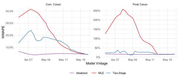
Figure 7: Prediction errors by model vintage, for regions that have peaked by May 21, 2020. Colors denote different approaches to learning $N_{i}$.

At one extreme, Idealized exhibits consistently low error even for early model vintages. This bears out the prediction of Theorem 3.8: given $N$, $\beta$ is easy to learn even early in the infection with few samples. MLE performs poorly until close to the target date of May 21 at which point sufficient data is available to learn $N$. This empirically illustrates the difficulty of learning $N$, as described in Theorem 3.3. Finally, we see that Two-Stage significantly outperforms MLE far away from the test date. Close to the test date the two approaches are comparable. For maximum daily infections, MLE drastically underperforms Two-Stage far from the test date. Our approach to learning from peaked regions significantly mitigates the difficulty of learning $N$. Further details on this study can be found in Appendix F.

6 Conclusion

In this paper, we have shown fundamental limits to learning for the SIR and Bass models, two models that often serve as building blocks for epidemic and product adoption modeling. By establishing sample complexity lower bounds, we have demonstrated the challenge of achieving early accurate forecasting due to the due to the time required to collect a sufficient number of observations. Moreover, our analysis extends to decision-making scenarios involving costly interventions to mitigate further infections, where we establish a lower bound on regret.

These findings highlight the difficulty of accurate forecasting based solely on infection trajectories and emphasize the need to incorporate additional data sources. We illustrate the potential benefits of seroprevalance testing, showing that even a sublinear-sized test, after a sufficient number of diffusion process samples, can significantly improve the estimation of $N$. Additionally, we introduce a heuristic approach employed in COVID-19 forecasting that biases the estimation of $N$ using a prior, leveraging regional infection timing heterogeneity. Going forward, we believe that the development of new methods that can effectively overcome the established lower bounds represent a valuable avenue for future research.

Appendices A, B and C contain the proofs of Theorems 3.4, 3.7 and 3.8 respectively. Appendix D contains the proofs of Propositions 2.1, 2.2, 3.5 and 3.6, each in their own subsections. Appendix E provides details on the datasets used in Section 5, and Appendix F contains a detailed description of the COVID-19 forecasting model from Section 5.4.

Appendix A Proof of Theorem 3.4

We finish the sections of the proof that were not included in the main paper. This includes the proof of Lemma 4.6, Lemma 4.8, calcuations for Lemma 4.7, and details regarding the final step of the proof.

We define $\lambda(N,k-1,C_{k-1})=\left(\frac{\beta(N-C_{k-1})}{N}+\gamma\right)I_{k-1}$ and $\eta(N,C_{k-1})=\frac{\beta(N-C_{k-1})}{\beta(N-C_{k-1})+N\gamma}$. Thus, for $k\leq\tau$, $\lambda(N,k-1,C_{k-1})$ is the mean of the $k$-th inter-arrival time and $\eta(N,C_{k-1})$ is the probability that the arrival in the $k$-th instance is a new infection rather than a recovery.

A.1 Proof of Lemma 4.6

Proof.

Suppose $k<\tau$ i.e $E_{k}=1$. Then, $k$ is equal to total number of jumps that have occurred so far (the number of movements from S to I and from I to R). The number of individuals that have moved from S to I is $C_{k}-I_{0}-R_{0}$, and the number of movements from I to R is $C_{k}-I_{k}-R_{0}$. Therefore, $k=2C_{k}-I_{0}-I_{k}-2R_{0}$. Since $I_{k}>0$, $C_{k}>r_{k}$.

Suppose $k\geq\tau$ i.e $E_{k}=0$. Then, $k$ is greater than or equal to the total number of jumps, which is still equal to $2C_{k}-I_{0}-I_{k}-2R_{0}$. Hence $C_{k}\leq r_{k}$ in this case.

$\square$

A.2 Proof of Lemma 4.8

Proof.

Let $X_{k}\overset{iid}{\sim}\text{Bern}(p)$ for $k=1,2,\dots$. Let $\{A_{k}:k\geq 0\}$ be a stochastic process defined by:

$$A_{k} =\begin{cases}C_{0}&\text{if }k=0\\ C_{0}+X_{1}+\dots+X_{k}&\text{if $A_{i}>r_{i}\;\forall i<k$}\\ A_{k-1}&\text{otherwise.}\\ \end{cases}$$

Let $\tau_{A}=\min\{k:A_{k}\leq r_{k}\}$ be the ‘‘stopping time’’ of this process.

Claim A.1.

$\Pr(\tau\leq m)\leq\Pr(\tau_{A}\leq m)$.

The proof of this claim involves showing the process $\{A_{k}\}$ is stochastically less than $\{C_{k}\}$; the proof can be found in Section A.2.1. We now upper bound $\Pr(\tau_{A}\leq m)$. $\tau_{A}\leq m$ if and only if $A_{k}\leq r_{k}$ for some $k\leq m$. Before this happens, $A_{k}=C_{0}+X_{1}+\dots+X_{k}$. Therefore, if $\tau_{A}\leq m$, it must be that $C_{0}+X_{1}+\dots+X_{k}\leq\frac{k+I_{0}+2R_{0}}{2}$ for some $k\leq m$.

$$\Pr(\tau_{A}\leq m) \leq\sum_{k=1}^{m}\Pr\left(C_{0}+X_{1}+\dots+X_{k}\leq\frac{k+I_{0}+2R_{0}}{2}\right)$$

$$=\sum_{k=1}^{m}\Pr\left(X_{1}+\dots+X_{k}<pk\left(1-\frac{2pk-k+I_{0}}{2pk}\right)\right).$$

Since $\mathbb{E}[X_{1}+\dots+X_{k}]=pk$, using the Chernoff bound (multiplicative form: $\Pr(\sum_{i=1}^{k}X_{i}\leq(1-\delta)\mu)\leq\exp(-\delta^{2}\mu/2)$) gives

$$\Pr(\tau_{A}\leq m) \leq\sum_{k=1}^{m}\exp\left(-\frac{pk}{2}\left(\left(1-\frac{1}{2p}\right)+\frac{I_{0}}{2pk}\right)^{2}\right)$$

$$=\sum_{k=1}^{m}\exp\left(-\frac{pk}{2}\left(1-\frac{1}{2p}\right)^{2}-\frac{I_{0}}{2}\left(1-\frac{1}{2p}\right)-\frac{I_{0}^{2}}{8pk}\right)$$

$$\leq\sum_{k=1}^{m}\exp\left(-\frac{pk}{2}\left(1-\frac{1}{2p}\right)^{2}-\frac{I_{0}}{2}\left(1-\frac{1}{2p}\right)\right)$$

$$\leq\exp\left(-\left(\frac{1}{2}-\frac{1}{4p}\right)I_{0}\right)\sum_{k=1}^{m}\exp\left(-\frac{pk}{2}\left(1-\frac{1}{2p}\right)^{2}\right)$$

(15) $$\leq C_{1}\exp(-C_{2}I_{0}),$$

for constants $C_{1}=\sum_{k=1}^{\infty}\exp\left(-\frac{pk}{2}\left(1-\frac{1}{2p}\right)^{2}\right),C_{2}=\frac{1}{2}-\frac{1}{4p}>0$. ($C_{1}$ is a constant since it is a geometric series with a ratio smaller than 1, since $p>1/2$.) Let $D$ be the solution to $C_{1}\exp(-C_{2}D)=\frac{1}{2}$. Then, if $I_{0}\geq D$, $\Pr(E_{m})=1-\Pr(\tau\leq m)\geq 1-\Pr(\tau_{A}\leq m)\geq\frac{1}{2}$.

$\square$

A.2.1 Proof of Claim A.1.

Definition A.2.

For scalar random variables $X,Y$, we say that $X$ is stochastically less than $Y$ (written $X\leq_{st}Y$) if for all $t\in\mathbb{R}$,

$$\Pr(X>t)\leq\Pr(Y>t).$$

For random vectors $X,Y\in\mathbb{R}^{n}$ we say that $X\leq_{st}Y$ if for all increasing functions $\phi:\mathbb{R}^{n}\rightarrow\mathbb{R}$,

$$\phi(X_{1},\dots,X_{n})\leq_{st}\phi(Y_{1},\dots,Y_{n}).$$

We make use of the following known result for establishing stochastic order for stochastic processes.

Theorem A.3 (Veinott 1965).

Suppose $X_{1},\dots,X_{n}$, $Y_{1},\dots,Y_{n}$ are random variables such that $X_{1}\leq_{st}Y_{1}$ and for any $x\leq y$,

$$(X_{k}|X_{1}=x_{1},\dots,X_{k-1}=x_{k-1})\leq_{st}(Y_{k}|Y_{1}=y_{1},\dots,Y_{k-1}=y_{k-1})$$

for every $2\leq k\leq n$. Then, $(X_{1},\dots,X_{n})\leq_{st}(Y_{1},\dots,Y_{n})$.

Proof of Claim A.1.

Because of the condition $\frac{\beta(N-m-C_{0})}{\beta(N-m-C_{0})+N\gamma}>p$, for $k\leq m$ and $k\leq\tau$, $C_{k}-C_{k-1}\sim\text{Bern}(q)$ for $q>p$. First, we show $(A_{0},A_{1},\dots,A_{m})\leq_{st}(C_{0},C_{1},\dots,C_{m})$ using Theorem A.3. $C_{0}\leq_{st}A_{0}$ since $C_{0}=A_{0}=I_{0}$. We condition on $A_{k-1}=x$ and $C_{k-1}=y$ for $x\leq y$, and we must show $A_{k}\leq_{st}C_{k}$. (We do not need to condition on all past variables since the both processes are Markov.) If $x\leq r_{k-1}$, then $A_{k}=A_{k-1}=x\leq y=C_{k-1}\leq C_{k}$. Otherwise, the process $A_{k}$ has not stopped, and neither has $C_{k}$ since $y\geq x$. Then, $A_{k}\sim x+\text{Bern}(p)$ and $C_{k}\sim y+\text{Bern}(q)$ for some $q\geq p$. Clearly, $A_{k}\leq_{st}C_{k}$ in this case. We apply Theorem A.3, which implies $A_{m}\leq_{st}C_{m}$.

Define the function $u:\mathbb{R}^{m+1}\rightarrow\{0,1\}$, $u(x_{0},x_{1},\dots,x_{m})=\mathds{1}\{\cup_{k=1}^{m}\{x_{k}\leq r_{k}\}\}$. Then, $u(A_{0},A_{1},\dots,A_{m})=1$ if and only if $\tau_{A}\leq m$, and $u(C_{0},C_{1},\dots,C_{m})=1$ if and only if $\tau\leq m$. $u$ is a decreasing function. Therefore, $u(A_{0},A_{1},\dots,A_{m})\geq_{st}u(C_{0},C_{1},\dots,C_{m})$. Then, $\Pr(\tau\leq m)=\Pr(u(C_{0},C_{1},\dots,C_{m})\geq 1)\leq\Pr(u(A_{0},A_{1},\dots,A_{m})\geq 1)=\Pr(\tau_{A}\leq m)$ as desired. $\square$

A.3 Calculations for Lemma 4.7

We define $\lambda(N,k-1,C_{k-1})=\left(\frac{\beta(N-C_{k-1})}{N}+\gamma\right)I_{k-1}$ and $\eta(N,C_{k-1})=\frac{\beta(N-C_{k-1})}{\beta(N-C_{k-1})+N\gamma}$. Thus, for $k\leq\tau$, $\lambda(N,k-1,C_{k-1})$ is the mean of the $k$-th inter-arrival time and $\eta(N,C_{k-1})$ is the probability that the arrival in the $k$-th instance is a new infection rather than a recovery.

Derivation of $\mathbb{E}_{C_{k}}[g_{C_{k}|C_{k-1}}(C_{k},C_{k-1},N)|E_{k-1}=1]$. When $E_{k-1}=1$, we have $C_{k}\sim C_{k-1}+\text{Bern}(\eta(N,C_{k-1}))$. Therefore, $\mathbb{E}_{C_{k}}[g_{C_{k}|C_{k-1}}(C_{k},C_{k-1},N)|E_{k-1}=1]=\mathcal{J}_{C_{k}\sim\text{Bern}(\eta(N,C_{k-1}))}(N)$. We reparameterize to write the Fisher information as:

$$\mathbb{E}_{C_{k}}[g_{C_{k}|C_{k-1}}(C_{k},C_{k-1},N)|E_{k-1}=1] =\mathcal{J}_{C_{k}\sim\text{Bern}(\eta)}(\eta)\left(\frac{\partial}{\partial N}\eta(N,C_{k-1})\right)^{2}$$

$$=\frac{1}{\eta(1-\eta)}\left(\frac{\partial}{\partial N}\eta(N,C_{k-1})\right)^{2}.$$

Use $\eta(N,C_{k-1})=\frac{\beta(N-C_{k-1})}{\beta(N-C_{k-1})+N\gamma}$ to derive

$$\frac{\partial}{\partial N}\eta(N,C_{k-1}) =\frac{\beta(\beta(N-C_{k-1})+\gamma N)-\beta(N-C_{k-1})(\beta+\gamma)}{(\beta(N-C_{k-1})+\gamma N)^{2}}$$

$$=\frac{\beta\gamma C_{k-1}}{(\beta(N-C_{k-1})+\gamma N)^{2}}.$$

Also, $\frac{1}{\eta(1-\eta)}=\frac{(\beta(N-C_{k-1})+N\gamma)^{2}}{(N-C_{k-1})\beta N\gamma}$.

Substituting,

$$\mathbb{E}_{C_{k}}[g_{C_{k}|C_{k-1}}(C_{k},C_{k-1},N)|E_{k-1}=1] =\frac{(\beta(N-C_{k-1})+N\gamma)^{2}}{(N-C_{k-1})\beta N\gamma}\left(\frac{\beta\gamma C_{k-1}}{(\beta(N-C_{k-1})+\gamma N)^{2}}\right)^{2}$$

$$=\frac{\beta\gamma C_{k-1}^{2}}{(N-C_{k-1})N(\beta(N-C_{k-1})+\gamma N)^{2}}$$

Derivation of $\mathbb{E}_{T_{k}}[g_{T_{k}|C_{k-1}}(T_{k},C_{k-1},N)|E_{k-1}=1]$. Similarly, conditioned on $E_{k-1}=1,T_{k}\sim\text{Exp}(\lambda(N,k-1,C_{k-1}))$. Therefore, $\mathbb{E}_{T_{k}}[g_{T_{k}|C_{k-1}}(T_{k},C_{k-1},N)]=\mathcal{J}_{T_{k}\sim\text{Exp}(\lambda(N,k-1,C_{k-1}))}(N)$. We reparameterize to write

$$\mathbb{E}_{T_{k}}[g_{T_{k}|C_{k-1}}(T_{k},C_{k-1},N)] =\mathcal{J}_{T_{k}\sim\text{Exp}(\lambda)}(\lambda)\left(\frac{\partial}{\partial N}\lambda(N,k-1,C_{k-1})\right)^{2}$$

$$=\frac{1}{\lambda^{2}}\left(\frac{\partial}{\partial N}\lambda(N,k-1,C_{k-1})\right)^{2}.$$

Use $\lambda(N,k-1,C_{k-1})=(\frac{\beta(N-C_{k-1})}{N}+\gamma)(2C_{k-1}-(k-1)-I_{0}-2R_{0})$ to derive

$$\frac{\partial}{\partial N}\lambda(N,k-1,C_{k-1}) =\frac{\beta C_{k-1}(2C_{k-1}-(k-1)-I_{0}-2R_{0})}{N^{2}}$$

$$\frac{1}{\lambda(N,k-1,C_{k-1})} =\frac{N}{(\beta(N-C_{k-1})+\gamma N)(2C_{k-1}-(k-1)-I_{0}-2R_{0})}.$$

Substituting,

$$\mathbb{E}_{T_{k}}[g_{T_{k}|C_{k-1}}(T_{k},C_{k-1},N)] =\left(\frac{\beta C_{k-1}}{N(\beta(N-C_{k-1})+\gamma N)}\right)^{2}$$

Derivation of $\mathcal{J}_{O_{m}}(N)$. Using the expressions derived above for $\mathbb{E}_{C_{k}}[g_{C_{k}|C_{k-1}}(C_{k},C_{k-1},N)|E_{k-1}=1]$ and
$\mathbb{E}_{T_{k}}[g_{T_{k}|C_{k-1}}(T_{k},C_{k-1},N)]$, we get

$$\mathbb{E}_{C_{k}}[g_{C_{k}|C_{k-1}}(C_{k},C_{k-1},N)|E_{k-1}=1]+\mathbb{E}_{T_{k}}[g_{T_{k}|C_{k-1}}(T_{k},C_{k-1},N)]$$

$$=\frac{\beta\gamma C_{k-1}^{2}}{(N-C_{k-1})N(\beta(N-C_{k-1})+\gamma N)^{2}}+\left(\frac{\beta C_{k-1}}{N(\beta(N-C_{k-1})+\gamma N)}\right)^{2}$$

$$=\frac{C_{k-1}^{2}}{(N-C_{k-1})N^{2}(N-C_{k-1}+\frac{\gamma}{\beta}N)}$$

Thus,

$$\mathcal{J}_{O_{m}}(N) =\sum_{k=1}^{m}\mathbb{E}[g_{C_{k}|C_{k-1}}(C_{k},C_{k-1},N)+g_{T_{k}|C_{k-1}}(T_{k},C_{k-1},N)|E_{k-1}=1]\Pr(E_{k-1}=1)$$

$$=\sum_{k=1}^{m}\mathbb{E}\left[\frac{C_{k-1}^{2}}{(N-C_{k-1})N^{2}(N-C_{k-1}+\frac{\gamma}{\beta}N)}\;\bigg{|}\;E_{k-1}=1\right]\Pr(E_{k-1}=1).$$

A.4 Details of Final Step of Theorem 3.4

Define $p\triangleq\frac{1}{2}(\frac{\beta}{\beta+\gamma}+\frac{1}{2})>\frac{1}{2}$ as in Lemma 4.8. Assume $N$ is large enough so that $m+C_{0}\leq\frac{N}{2}$ and $\frac{\beta(N-m-C_{0})}{\beta(N-m-C_{0})+P\gamma}>p$ (this is possible since $\frac{\beta}{\beta+\gamma}>p$ and $m=o(N)$).

For the upper bound, we have that $C_{k}\leq k+I_{0}+R_{0}$ by definition. Since $I_{0},R_{0}\leq m$ by assumption, $C_{k}\leq 3m$. Moreover, by assumption, $C_{k}\leq m+C_{0}\leq\frac{N}{2}$. Plugging these into (11) results in

$$\mathcal{J}_{O_{m}}(N) \leq\sum_{k=0}^{m-1}\Pr(E_{k-1}=1)\frac{(3m)^{2}}{N^{2}(N-\frac{1}{2}N)((N-\frac{1}{2}N)+\frac{\gamma}{\beta}N)}\leq H_{1}\frac{m^{3}}{N^{4}},$$

for a constant $H_{1}$.

Then, similarly to the upper bound, $\mathcal{J}_{O_{m}}(N)\geq H_{2}\frac{m^{3}}{N^{4}}$ follows from using $\Pr(E_{m}=1)\geq\frac{1}{2}$ and the fact that $C_{k}\geq\frac{k+I_{0}+2R_{0}}{2}\geq\frac{k}{2}$ when $E_{k}=1$ (Lemma 4.6):

$$\mathcal{J}_{O_{m}}(N) \geq\sum_{k=0}^{m-1}\frac{1}{2}\frac{\left(\frac{k}{2}\right)^{2}}{N^{4}}\geq H_{2}\frac{m^{3}}{N^{4}},$$

Combining the upper and lower bounds finish the proof.

A.5 Generalization of Theorem 3.3: a Finite-sample Result

Note that the proof of Theorem 3.4 provides exact formulas for the Fisher information, where quantities such as $N$ and $m$ are finite. This leads to the following result of which Theorem 3.3 is a special case, and it holds for any initial conditions $I_{0}$ and $R_{0}.$

Theorem A.4.

Consider any observation $(T_{0},I_{0},R_{0},T_{1},I_{1},R_{1},\dotsc,T_{m},I_{m},R_{m})$ from either a Bass model or an SIR model (with any initial $I_{0}$ and $R_{0}$). Suppose $\hat{N}$ is an un-biased estimator for $N$. Let $I_{\max}=\max_{1\leq i\leq m}I_{i}$ with $I_{\max}\leq c(p,\gamma,\beta)N.$ Then

$$\mathbb{E}\left[\frac{(\hat{N}-N)^{2}}{N^{2}}\right]\geq C(p,\gamma,\beta)\frac{N^{2}}{I_{\max}^{3}}$$

where $C(p,\gamma,\beta)$ and $c(p,\gamma,\beta)$ are constants that are explicit functions of $p,\gamma,\beta$.

Appendix B Proof of Theorem 3.7

Proof.

We construct the estimators $\hat{a}$ for $a$ and $\hat{\beta}$ for $\beta$ as the following. To begin, let

$$\hat{A} :=\frac{\sum_{i=1}^{m/2}\min(T_{i},T_{m-i})}{m/2}$$

$$\hat{B} :=\frac{\sum_{i=1}^{m/4}\min(T_{i},T_{m/2-i})}{m/4}.$$

We will show momentarily that $\hat{A}$ approximates $\frac{1}{2a+m\beta}$ and $\hat{B}$ approximates $\frac{1}{2a+(m/2)\beta}$. We then construct $\hat{a}$ and $\hat{\beta}$:

$$\hat{\beta} :=\left(\frac{1}{\hat{A}}-\frac{1}{\hat{B}}\right)\frac{2}{m}$$

$$\hat{a} :=\left(\frac{2}{\hat{B}}-\frac{1}{\hat{A}}\right)\frac{1}{2}.$$

To start the proof, let us analyze $\hat{A}$. Let $A_{i}=\min(T_{i},T_{m-i}),1\leq i\leq\lfloor m/2\rfloor$. By the property of independent exponential random variables, we have $A_{i}\sim\mathrm{Exp}(l_{i})$ where

$$l_{i}:=(2a+\beta m)-(a+i\beta)\frac{i}{N}-(a+(m-i)\beta)\frac{m-i}{N}.$$

Note that when $N\gg m$, we shall have $l_{i}\approx 2a+\beta m$, which is independent from $i$. This inspires us to use $\hat{A}:=\frac{\sum_{i}A_{i}}{m/2}$ as an estimator for $\frac{1}{2a+\beta m}.$

More specifically, Let $\mu=\frac{\sum_{i}E[A_{i}]}{m/2}=\frac{1}{m/2}\sum_{i}\frac{1}{l_{i}}$. Note that

$$\frac{N-m}{N}(2a+\beta m)\leq l_{i}\leq 2a+\beta m.$$

Then, this implies that $\mu$ is close to $\frac{1}{2a+\beta m}$:

(16) $$\frac{1}{2a+m\beta}\leq\mu\leq\frac{N}{N-m}\frac{1}{2a+m\beta}$$

On the other hand, we can invoke the multiplicative Bernstein inequality (Janson (2018)) to obtain, with probability $1-O(1/N^{2})$,

(17) $$(1-\delta)\mu\leq\hat{A}\leq\mu(1+\delta)$$

where $\delta:=O(\sqrt{\log(N)/m}).$ Combining Eq. 16 and Eq. 17, we then have

$$\frac{1}{2a+m\beta}(1-\delta)\leq\hat{A}\leq\frac{N}{N-m}(1+\delta)\frac{1}{2a+m\beta}.$$

This further implies desired bounds for using $\frac{1}{\hat{A}}$ to estimate $2a+m\beta$:

$$\left|\frac{1}{\hat{A}}-(2a+m\beta)\right| \lesssim(\delta+\frac{m}{N})(2a+m\beta)$$

$$\lesssim\sqrt{\frac{\log(N)}{m}}(2a+m\beta)$$

where the last inequality uses $m=O(N^{2/3}\log^{1/3}(N))$ (hence $m/N\lesssim\delta$).

A similar analysis can be conducted for $\hat{B}$, which implies that

$$\left|\frac{1}{\hat{B}}-(2a+(m/2)\beta)\right| \lesssim(\delta+\frac{m}{N})(2a+(m/2)\beta)$$

$$\lesssim\sqrt{\frac{\log(N)}{m}}(2a+(m/2)\beta)$$

Combining the bounds of $\hat{A}$ and $\hat{B}$, we then obtain the bounds for $\hat{a}$ and $\hat{\beta}$, which completes the proof. $\square$

Appendix C Proof of Theorem 3.8

C.1 Construction of Estimators

Our construction of estimators $\hat{\beta}$ for $\beta$ and $\hat{\gamma}$ for $\gamma$ is the following. To begin, let

$$\hat{A}:=\frac{C_{m}-C_{0}}{m}$$

$$\hat{B}:=\frac{\sum_{k=1}^{\min(m,\tau)}I_{k-1}T_{k}}{m}.$$

We will show momentarily that $\hat{A}$ can be viewed as an estimator for $\frac{\beta}{\beta+\gamma}$ and $\hat{B}$ an estimator for $\frac{1}{\beta+\gamma}.$ Then given $\hat{A}$ and $\hat{B}$, we construct

$$\hat{\beta}:=\frac{\hat{A}}{\hat{B}}$$

$$\hat{\gamma}:=\frac{1}{\hat{B}}-\hat{\beta}.$$

This construction leads to the guarantees stated in Theorem 3.8.

The proof is based on a series of lemmas stated below. The first lemma bounds the probability that the epidemic diminishes before $m$ samples, which follows from (15) of the proof of Lemma 4.8.

Lemma C.1.

If $\frac{\beta}{\beta+\gamma}\frac{N-m-C_{0}}{N}>p$, $\Pr(\tau<m)\leq B_{1}e^{-B_{2}I_{0}}$, where $B_{1},B_{2}>0$ are constant that depend only on $\beta$ and $\gamma$.

The next two lemmas give a high probability confidence bound for estimators $\hat{A}$ and $\hat{B}$.

Lemma C.2.

For any $m,I_{0}$ where $\frac{\beta}{\beta+\gamma}\frac{N-m-C_{0}}{N}>\frac{1}{2}$, for any $\delta>0$,

$$\Pr\left(\frac{C_{m}-C_{0}}{m}\notin\left[\frac{\beta}{\beta+\gamma}(1-\delta)\frac{N-m-C_{0}}{N},\frac{\beta}{\beta+\gamma}(1+\delta)\right],\tau\geq m\right)\leq 2\exp(-m\delta^{2}/(4+2\delta)).$$

Lemma C.3.

Let $\tilde{S}_{m}=\sum_{k=1}^{\min(m,\tau)}I_{k-1}T_{k}$. Then

$$\Pr\left(\frac{\tilde{S}_{m}}{m}\notin[\frac{(1-\delta)}{\beta+\gamma},\frac{(1+\delta)}{\beta+\gamma}\frac{N}{N-m-C_{0}}],\tau\geq m\right)\leq 2e^{-m\frac{N-m-C_{0}}{N}(\delta-\ln(1+\delta))}.$$

The next proposition combines the two estimators from the above lemmas and into estimators $\hat{\beta}$ and $\hat{\gamma}$.

Proposition C.4.

Assume $\beta>\gamma>0$. Let $I_{0}\leq m<N$ such that $\frac{\beta}{\beta+\gamma}\frac{N-m-C_{0}}{N}>p$. Let $z=\frac{N-m-C_{0}}{N}$. Then, for any $0<\delta<1$, with probability $1-4e^{-m(\delta-\ln(1+\delta))}-4e^{-m\delta^{2}/(4+2\delta)}-2B_{1}e^{-B_{2}I_{0}}$,

(18) $$\hat{\beta} \in\left[\beta\frac{(1-\delta)z^{2}}{1+\delta},\beta\frac{1+\delta}{1-\delta}\right]$$

(19) $$\hat{\gamma} \in\left[\gamma\frac{z}{1+\delta}+\beta\frac{(1-\delta)z-(1+\delta)^{2}}{(1+\delta)(1-\delta)},\gamma\frac{1}{1-\delta}+\beta\frac{1+\delta-(1-\delta)^{2}z^{2}}{(1-\delta)(1+\delta)}\right],$$

where $B_{1},B_{2}>0$ are constants that depend on $\beta$ and $\gamma$.

We first show Theorem 3.8 using these results. We then prove Lemma C.2, Lemma C.3, and Proposition C.4 in Section C.3.

C.2 Proof of Theorem 3.8

Proof.

Let $\delta=\sqrt{\frac{5\log m}{m}}$. First, we claim that the probability in Proposition C.4 is greater than $1-\frac{8}{m}-2B_{1}e^{-B_{2}I_{0}}$. Note that $\ln(1+\delta)\leq\delta-\frac{\delta^{2}}{2}+\delta^{3}$, implying $\delta-\ln(1+\delta)\geq\delta^{2}(\frac{1}{2}-\delta)$. Since $\delta\leq\frac{1}{4}$,

$$4e^{-m(\delta-\ln(1+\delta)} \leq 4e^{-m\frac{\delta^{2}}{4}}\leq\frac{4}{m}.$$

Using $\delta\leq\frac{1}{4}$ again,

$$4e^{-m\delta^{2}/(4+2\delta)} \leq 4e^{-m\frac{\delta^{2}}{5}}=\frac{4}{m}.$$

Hence, the bound in C.4 holds with probability greater than $1-\frac{8}{m}-2B_{1}e^{-B_{2}I_{0}}$.

Since we assume $m(m+C_{0})\leq N$ and $z=1-\frac{m+C_{0}}{N}$,

(20) $$1-z\leq\frac{1}{m}.$$

From here on, assume the confidence bounds (18)-(19) hold. Note that $\frac{1+\delta}{1-\delta}\leq 1+3\delta$ and $\frac{1-\delta}{1+\delta}\geq 1-3\delta$ for $\delta<\frac{1}{4}$. Then,

$$(\hat{\beta}-\beta)^{2} \leq\beta^{2}\left(1+3\delta-(1-3\delta)z^{2}\right)^{2}$$

$$\leq\beta^{2}\left((1-z)+3\delta(1+z)\right)^{2}$$

$$\leq\beta^{2}\left(\frac{1}{m}+6\sqrt{\frac{5\log m}{m}}\right)^{2}$$

$$\leq\beta^{2}M_{3}\frac{\log m}{m}$$

for an absolute constant $M_{3}>0$. The second last step uses (20) and $1+z\leq 2$. Therefore, $\mathrm{RelError}(\hat{\beta},\beta)\leq M_{1}\frac{\log m}{m}$.

Similarly,

(21) $$(\hat{\gamma}-\gamma)^{2} \leq\left(\gamma\left(\frac{1}{1-\delta}-\frac{z}{1+\delta}\right)+\beta\left(\frac{1+\delta-(1-\delta)^{2}z^{2}}{(1-\delta)(1+\delta)}-\frac{(1-\delta)z-(1+\delta)^{2}}{(1+\delta)(1-\delta)}\right)\right)^{2}.$$

Using the fact that $(1-\delta)(1+\delta)\geq\frac{1}{2}$,

$$\frac{1}{1-\delta}-\frac{z}{1+\delta}\leq 2((1-z)+\delta(1+z))\leq 2\left(\frac{1}{m}+2\sqrt{\frac{5\log m}{m}}\right).$$

$$\frac{1+\delta-(1-\delta)^{2}z^{2}}{(1-\delta)(1+\delta)}-\frac{(1-\delta)z-(1+\delta)^{2}}{(1+\delta)(1-\delta)} =\frac{(1+\delta)-(1-\delta)z+(1+\delta)^{2}-(1-\delta)^{2}z^{2}}{1-\delta^{2}}$$

$$\leq 2(1-z)+4\delta(1+z)+\frac{1+\delta}{1-\delta}-\frac{1-\delta}{1+\delta}z^{2}$$

$$\leq 2(1-z)+8\delta+(1+3\delta)-(1-3\delta)z^{2}$$

$$\leq 2(1-z)+8\delta+(1-z^{2})+6\delta(1+z^{2})$$

$$\leq(1-z)(3+z)+\delta(8+6(1+z^{2}))$$

$$\leq\frac{4}{m}+20\sqrt{\frac{5\log m}{m}}.$$

Substituting back into (21) results in

$$(\hat{\gamma}-\gamma)^{2} \leq\left(\gamma\left(\frac{2}{m}+4\sqrt{\frac{5\log m}{m}}\right)+\beta\left(\frac{4}{m}+20\sqrt{\frac{5\log m}{m}}\right)\right)^{2}$$

$$\leq M_{2}\beta^{2}\frac{\log m}{m},$$

for an absolute constant $M_{2}$, since $\beta>\gamma$. This implies the desired result. $\square$

C.3 Proofs of Intermediate Results

C.3.1 Proof of Lemma C.2.

Proof.

Fix $m$, let $z:=\frac{N-m-C_{0}}{N},p=\frac{\beta}{\beta+\gamma}z$. Then $p>\frac{1}{2}.$ Define three stochastic processes $\{A_{k}:k\geq 0\}$, $\{B_{k}:k\geq 0\}$, $\{\tilde{C}_{k}:k\geq 0\}$:

$$A_{k} =\begin{cases}C_{0}&\text{if }k=0\\ A_{k-1}+\text{Bern}(p)&\text{otherwise}.\\ \end{cases}$$

$$B_{k} =\begin{cases}C_{0}&\text{if }k=0\\ B_{k-1}+\text{Bern}(p/z)&\text{otherwise}.\\ \end{cases}$$

$$\tilde{C}_{k} =\begin{cases}C_{0}&\text{if }k=0\\ \tilde{C}_{k-1}+\text{Bern}\left\{\frac{\beta(N-\tilde{C}_{k-1})}{\beta(N-\tilde{C}_{k-1})+N\gamma}\right\}&\text{otherwise}.\\ \end{cases}$$

Note that $\tilde{C}_{k}$ is a modified version of $C_{k}$ where $\tilde{C}_{k}$ still evolves after the stopping time.

Claim C.5.

$A_{m}$ is stochastically less than $\tilde{C}_{m}$ ($A_{m}\leq_{st}\tilde{C}_{m}$); $\tilde{C}_{m}$ is stochastically less than $B_{m}$ ($\tilde{C}_{m}\leq_{st}B_{m}$); that is, for any $\ell\in\mathbb{R}$,

$$\Pr(B_{m}\leq\ell)\leq\Pr(\tilde{C}_{m}\leq\ell)\leq\Pr(A_{m}\leq\ell).$$

This claim follows from Theorem A.3, using a similar argument to A.1.

Let $A_{k}=C_{0}+X_{1}+X_{2}+\dotsc X_{k}$ where $X_{i}\sim\text{Bern}(p)$ are independent. We provide the left tail bound for $C_{m}$. Note that when $\tau\geq m$, $C_{m}\overset{d}{=}\tilde{C}_{m}.$ Hence,

$$\Pr(C_{m}\leq mp(1-\delta)+C_{0},\tau\geq m) =\Pr(\tilde{C}_{m}\leq mp(1-\delta)+C_{0},\tau\geq m)$$

$$\leq\Pr(\tilde{C}_{m}\leq mp(1-\delta)+C_{0})$$

(22) $$\leq\Pr(A_{m}\leq mp(1-\delta)+C_{0}).$$

Using the Chernoff bound gives,

$$\Pr(A_{m}\leq mp(1-\delta)+C_{0}) =\Pr(C_{0}+X_{1}+\dots+X_{m}\leq pm(1-\delta)+C_{0})$$

$$=\Pr\left(X_{1}+\dots+X_{m}\leq mp\left(1-\delta\right)\right)$$

$$\leq\exp\left(-\frac{mp}{2}\delta^{2}\right).$$

Therefore,

$$\Pr\left(\frac{C_{m}-C_{0}}{m}\leq\frac{p}{z}(1-\delta)z,\tau\geq m\right) =\Pr\left(C_{m}\leq mp(1-\delta)+C_{0},\tau\geq m\right)$$

$$\leq\exp\left(-\frac{mp}{2}\delta^{2}\right)\leq\exp(-m\delta^{2}/4).$$

Let $B_{k}=C_{0}+Y_{1}+\dotsc+Y_{k}$ where $Y_{i}\sim\text{Bern}(p/z)$ are independent. Similarly, for the upper tail bound, we have

$$\Pr\left(\frac{C_{m}-C_{0}}{m}\geq\frac{p}{z}(1+\delta),\tau\geq m\right) =\Pr(C_{m}\geq mp/z(1+\delta)+C_{0},\tau\geq m)$$

$$\leq\Pr(B_{m}\geq mp/z(1+\delta)+C_{0})$$

$$\leq\Pr(C_{0}+Y_{1}+\dots+Y_{m}\geq mp/z(1+\delta)+C_{0})$$

$$\leq\exp(-\frac{mp/z}{2+\delta}\delta^{2})\leq\exp(-m\delta^{2}/(4+2\delta))$$

due to the multiplicative Chernoff bound $\Pr(Z\geq E[Z](1+\delta))\leq e^{-\frac{Z}{2+\delta}\delta^{2}}$ where $Z$ is the sum of i.i.d Bernoulli random variables.

Combine upper and lower tail bounds and note that $p/z=\frac{\beta}{\beta+\gamma}$. Then, we can conclude, for any $\delta>0$,

$$\Pr\left(\frac{C_{m}-C_{0}}{m}\notin[\frac{\beta}{\beta+\gamma}(1-\delta)z,\frac{\beta}{\beta+\gamma}(1+\delta)],\tau\geq m\right)\leq 2\exp(-m\delta^{2}/(4+2\delta)).$$

$\square$

C.3.2 Proof of Lemma C.3.

Proof.

Conditioned on $(I_{0},C_{0},I_{1},C_{1},\dotsc,I_{m-1},C_{m-1})$ with $\tau\geq m$, we have

$$I_{k-1}T_{k}\sim\text{Exp}\left(\beta\frac{N-C_{k-1}}{N}+\gamma\right)$$

are independent exponential random variables.

Theorem 5.1 in Janson (2018) gives us a tail bound for the sum of independent exponential random variables: let $X=\sum_{i=1}^{n}X_{i}$ with $X_{i}\sim\text{Exp}(a_{i})$ independent, then for $\delta>0$,

(23) $$\Pr(X\geq(1+\delta)\mu) \leq\frac{1}{1+\delta}e^{-a_{*}\mu(\delta-\ln(1+\delta))}\leq e^{-a_{*}\mu(\delta-\ln(1+\delta))}$$

(24) $$\Pr(X\leq(1-\delta)\mu) \leq e^{-a_{*}\mu(\delta-\ln(1+\delta))}$$

where $\mu=E[X],a_{*}=\min_{1\leq i\leq n}a_{i}.$

Let $\tilde{S}_{m|\vec{C},\vec{I}}$ be $\tilde{S}_{m}$ conditioned on $(I_{0},C_{0},I_{1},C_{1},\dotsc,I_{m-1},C_{m-1})$ with $\tau\geq m$. Let $\mu=E[\tilde{S}_{m|\vec{C},\vec{I}}]=\sum_{k=1}^{m}\frac{1}{\beta(N-C_{k-1})/N+\gamma}$, $a_{*}=\min_{1\leq k\leq m}\beta(N-C_{k-1})/N+\gamma.$ It is easy to verify the following facts

$$\mu a_{*} \geq\sum_{k=1}^{m}\frac{a_{*}}{(\beta+\gamma)}\geq m\frac{N-m-C_{0}}{N}$$

$$\frac{1}{\beta+\gamma} \leq\frac{\mu}{m}\leq\frac{1}{\beta+\gamma}\frac{N}{N-m-C_{0}}.$$

Combining these with Eqs. 23 and 24, we have

$$\Pr\left(\frac{\tilde{S}_{m|\vec{C},\vec{I}}}{m}\notin\left[\frac{(1-\delta)}{\beta+\gamma},\frac{(1+\delta)}{\beta+\gamma}\frac{N}{N-m-C_{0}}\right]\right) \leq\Pr\left(\frac{\tilde{S}_{m|\vec{C},\vec{I}}}{m}\notin\left[\frac{\mu(1-\delta)}{m},\frac{\mu(1+\delta)}{m}\right]\right)$$

$$\leq 2e^{-m\frac{N-m-C_{0}}{N}(\delta-\ln(1+\delta))}.$$

Therefore,

$$\Pr\left(\frac{\tilde{S}_{m}}{m}\notin I,\tau\geq m\right) =\int_{\vec{C},\vec{I}|\tau\geq m}\Pr\left(\frac{\tilde{S}_{m}}{m}\notin I~{}|~{}\vec{C},\vec{I},\tau\geq m\right)f(\vec{C},\vec{I}|\tau\geq m)\Pr(\tau\geq m)$$

$$\leq 2e^{-m\frac{N-m-C_{0}}{N}(\delta-\ln(1+\delta))}\Pr(\tau\geq m)$$

$$\leq 2e^{-m\frac{N-m-C_{0}}{N}(\delta-\ln(1+\delta))}.$$

$\square$

C.3.3 Proof of Proposition C.4.

Proof.

Let $\hat{\beta}=\frac{C_{m}-C_{0}}{\tilde{S}_{m}},z=\frac{N-C_{0}-m}{N}$. Suppose $x\in\frac{\beta}{\beta+\gamma}[(1-\delta)z,1+\delta],y\in\frac{1}{\beta+\gamma}[1-\delta,(1+\delta)1/z]$. Then,

(25) $$\frac{x}{y}\in\left[\beta\frac{(1-\delta)z^{2}}{1+\delta},\beta\frac{1+\delta}{1-\delta}\right]$$

Similarly, let $\hat{\gamma}=\frac{m}{\tilde{S}_{m}}-\hat{\beta}.$ Suppose $a\in(\beta+\gamma)[\frac{z}{1+\delta},\frac{1}{1-\delta}],b\in\beta[\frac{(1-\delta)z^{2}}{1+\delta},\frac{1+\delta}{1-\delta}]$. Then

(26) $$a-b\in\left[\gamma\frac{z}{1+\delta}+\beta\frac{(1-\delta)z-(1+\delta)^{2}}{(1+\delta)(1-\delta)},\gamma\frac{1}{1-\delta}+\beta\frac{1+\delta-(1-\delta)^{2}z^{2}}{(1-\delta)(1+\delta)}\right].$$

Then, for any sets $U_{1},U_{2}$,

$$\Pr(\hat{\beta}\in U_{1},\hat{\gamma}\in U_{2}) \geq 1-\Pr(\hat{\beta}\notin U_{1})-\Pr(\hat{\gamma}\notin U_{2})$$

$$\geq 1-\Pr(\hat{\beta}\notin U_{1},\tau>m)-\Pr(\hat{\beta}\notin U_{2},\tau>m)-2\Pr(\tau<m)$$

$$\geq 1-4e^{-m(\delta-\ln(1+\delta))}-4e^{-m\delta^{2}/(4+2\delta)}-2B_{1}e^{-B_{2}I_{0}},$$

where the last step uses Lemma C.1, Lemma C.2 and Lemma C.3, using the intervals (25) and (26) for $U_{1}$ and $U_{2}$ respectively.

$\square$

Appendix D Proofs of Propositions

D.1 Proof of Proposition 2.1

Proof.

As in Miller (2017, 2012), the solution $\{(s^{\prime}(t),i^{\prime}(t),r^{\prime}(t)):t\geq 0\}$ can be written as:

$$s^{\prime}(t) =s^{\prime}(0)e^{-\xi^{\prime}(t)}$$

$$i^{\prime}(t) =N^{\prime}-s^{\prime}(t)-r^{\prime}(t)$$

$$r^{\prime}(t) =r(0)+\frac{\gamma^{\prime}N^{\prime}}{\beta^{\prime}}\xi^{\prime}(t)$$

$$\xi^{\prime}(t) =\frac{\beta^{\prime}}{N^{\prime}}\int_{0}^{t}i^{\prime}\left(t^{*}\right)dt^{*}$$

Making the appropriate substitutions yields the following equivalent system:

(27) $$i^{\prime}(t) =N^{\prime}-s^{\prime}(0)\exp\left(-\frac{\beta^{\prime}}{N^{\prime}}\xi(t)\right)-r(0)-\frac{\gamma^{\prime}N^{\prime}}{\beta^{\prime}}\xi^{\prime}(t)$$

(28) $$\xi^{\prime}(t) =\frac{\beta^{\prime}}{N^{\prime}}\int_{0}^{t}i^{\prime}\left(t^{*}\right)dt^{*}.$$

Therefore, it remains to show that for $\eta>0$, $\{(s(t),i(t),r(t)):t\geq 0\}\triangleq\{(\eta s^{\prime}(t),\eta i^{\prime}(t),\eta r^{\prime}(t)):t\geq 0\}$ is a solution for (27) and (28) where $N^{\prime}$ is replaced with $\eta N^{\prime}$. Starting with (27),

$$i^{\prime}(t) =N^{\prime}-s^{\prime}(0)\exp\left(-\xi^{\prime}(t)\right)-r^{\prime}(0)-\frac{\gamma^{\prime}N^{\prime}}{\beta^{\prime}}\xi^{\prime}(t)$$

$$\eta i^{\prime}(t) =\eta\left(N^{\prime}-s^{\prime}(0)\exp\left(-\xi^{\prime}(t)\right)-r^{\prime}(0)-\frac{\gamma^{\prime}N^{\prime}}{\beta^{\prime}}\xi^{\prime}(t)\right)$$

$$=\eta N^{\prime}-\alpha s^{\prime}(0)\exp\left(-\xi(t)\right)-\eta r(0)-\frac{\gamma^{\prime}\eta N^{\prime}}{\beta^{\prime}}\xi(t)$$

where $\xi(t)=\xi^{\prime}(t)=\frac{\beta^{\prime}}{N^{\prime}\eta}\int_{0}^{t}\eta i^{\prime}\left(t^{*}\right)dt^{*}$. Noting that $\xi^{\prime}(t)=\xi(t)$ and substituting $i(t)=\eta i^{\prime}(t)$ yields the equations below, clearly showing that $\{(s(t),i(t),r(t)):t\geq 0\}$ satisfy (27) and (28):

$$i(t) =\eta N^{\prime}-s(0)\exp\left(-\xi(t)\right)-r(0)-\frac{\gamma^{\prime}\eta N^{\prime}}{\beta^{\prime}}\xi(t)$$

$$\xi(t) =\frac{\beta^{\prime}}{N^{\prime}\eta}\int_{0}^{t}i\left(t^{*}\right)dt^{*}.$$

$\square$

D.2 Proof of Proposition 2.2

D.2.1 SIR Model

Proof.

Consider initial conditions $(s(0),i(0),0)$, as in Miller (2017, 2012), the analytical solution is given by

$$s(t) =s(0)e^{-\xi(t)},$$

$$i(t) =N-s(t)-r(t),$$

$$r(t) =\frac{\gamma\;N}{\beta}\xi(t),$$

$$\xi(t) =\frac{\beta}{N}\int_{0}^{t}i(t^{\prime})dt^{\prime}.$$

Consider two SIR models with parameters $(N,\beta,\gamma)$ and $(N^{\prime},\beta^{\prime},\gamma^{\prime})$, and initial conditions $(s_{0},i_{0},0)$ and $(s^{\prime}_{0},i^{\prime}_{0},0)$ respectively. We claim that infection trajectories $i(t)$ and $i^{\prime}(t)$ being identical on an open set $[0,T)$ implies the parameters and initial conditions are identical as well.

Assume $i(t)=i^{\prime}(t)$ for all $t\in[0,T)$; then, given the exact solution above it follows that

$$N-s_{0}e^{-\frac{\beta}{N}x}-\gamma x=N^{\prime}-s^{\prime}_{0}e^{-\frac{\beta^{\prime}}{N^{\prime}}x}-\gamma^{\prime}x, \text{ for all }x\in\Big{[}0,\int_{0}^{T}i(t)dt\Big{]}$$

As functions of $x$, both the RHS and LHS in the equality above are holomorphic, and hence, using the identity theorem, we then have for all $x\in\mathbb{R}$, there is $N-s_{0}e^{-\frac{\beta}{N}x}-\gamma x=N^{\prime}-s^{\prime}_{0}e^{-\frac{\beta^{\prime}}{N^{\prime}}x}-\gamma^{\prime}x$.

Then the following implies $\gamma=\gamma^{\prime}$:

$$-\gamma=\lim_{x\rightarrow+\infty}\frac{N-s_{0}e^{-\frac{\beta}{N}x}-\gamma x}{x}=\lim_{x\rightarrow+\infty}=\frac{N^{\prime}-s^{\prime}_{0}e^{-\frac{\beta^{\prime}}{N^{\prime}}x}-\gamma^{\prime}x}{x}=-\gamma^{\prime}.$$

Hence for all $x\in\mathbb{R}$, $N-s_{0}e^{-\frac{\beta}{N}x}=N^{\prime}-s^{\prime}_{0}e^{-\frac{\beta^{\prime}}{N^{\prime}}x}.$ Again, by taking $x$ to infinity, we can conclude $N=N^{\prime}$ by the following

$$N=\lim_{x\rightarrow+\infty}\left(N-s_{0}e^{-\frac{\beta}{N}x}\right)=\lim_{x\rightarrow+\infty}\left(N^{\prime}-s_{0}^{\prime}e^{-\frac{\beta^{\prime}}{N^{\prime}}x}\right)=N^{\prime}.$$

Furthermore, by taking $x=0$, we can also get $s_{0}=s_{0}^{\prime}$ and then $\beta=\beta^{\prime}$ follows. This completes the proof. $\square$

D.2.2 Bass Model

Proof.

Consider the initial condition $i(0)=0.$ By the analytic solution given by Bass (1969), we have

$$i(t)=N\frac{1-e^{-(p+\beta)t}}{\frac{\beta}{p}e^{-(p+\beta)t}+1}.$$

Consider two bass models with parameters $(N,\beta,p)$ and $(N^{\prime},\beta^{\prime},p^{\prime})$ and initial conditions $i(0)=0,i^{\prime}(0)=0$ respectively. We claim that trajectories $i(t)$ and $i^{\prime}(t)$ being identical on an open set $[0,T)$ implies the parameters are identical as well.

Assume $i(t)=i^{\prime}(t)$ for all $t\in[0,T)$; then, given the exact solution above it follows that

(29) $$N\frac{1-e^{-(p+\beta)t}}{\frac{\beta}{p}e^{-(p+\beta)t}+1}=N^{\prime}\frac{1-e^{-(p^{\prime}+\beta^{\prime})t}}{\frac{\beta^{\prime}}{p^{\prime}}e^{-(p^{\prime}+\beta^{\prime})t}+1}, \text{ for all }t\in[0,T)$$

As functions of $t$, both the RHS and LHS in the equality above are holomorphic, and hence, using the identity theorem, we then have Eq. 29 holds for all $t\in\mathbb{R}.$

By taking $t$ to infinity, we can easily obtain $N=N^{\prime}.$ Furthermore, taking the derivative for $t$ on both sides of Eq. 29, one can obtain

(30) $$\frac{(p+\beta)^{2}}{p}\frac{e^{-(p+\beta)t}}{(\beta/p\cdot e^{-(p+\beta)t}+1)^{2}}=\frac{(p^{\prime}+\beta^{\prime})^{2}}{p^{\prime}}\frac{e^{-(p^{\prime}+\beta^{\prime})t}}{(\beta^{\prime}/p^{\prime}\cdot e^{-(p^{\prime}+\beta^{\prime})t}+1)^{2}}.$$

By taking $t=0$ on both sides of Eq. 30, one can verify that $p=p^{\prime}.$ Furthermore, let $g(t)=\frac{(p+\beta)^{2}}{p}\frac{e^{-(p+\beta)t}}{(\beta/p\cdot e^{-(p+\beta)t}+1)^{2}}$ and $g^{\prime}(t)=\frac{(p^{\prime}+\beta^{\prime})^{2}}{p^{\prime}}\frac{e^{-(p^{\prime}+\beta^{\prime})t}}{(\beta^{\prime}/p^{\prime}\cdot e^{-(p^{\prime}+\beta^{\prime})t}+1)^{2}}.$

Note that

$$-(p+\beta)=\lim_{t\rightarrow+\infty}\frac{\ln(g(t))}{t}=\lim_{t\rightarrow+\infty}\frac{\ln(g^{\prime}(t))}{t}=-(p^{\prime}+\beta^{\prime}).$$

We then can conclude $\beta=\beta^{\prime}$. This completes the proof.

$\square$

D.3 Proof of Proposition 3.5

Proof.

Note that $\mathbb{E}[T_{i}]=\frac{N}{pN(N-i)+\beta i(N-i)}.$ Then

$$\mathbb{E}[t_{k^{\rm CR}}]=\mathbb{E}\left[\sum_{i=1}^{N^{2/3}-1}T_{i}\right]=\sum_{i=1}^{N^{2/3}-1}\frac{N}{pN(N-i)+\beta i(N-i)}.$$

Let $f(x)=\frac{N}{pN(N-x)+\beta x(N-x)}$, we use $f(x)$ as a proxy to bound $\mathbb{E}[t_{k^{\rm CR}}].$ Easy to verify that $f(x)$ is decreasing when $x\in(0,\mathring{r}]$ where $\mathring{r}=(1-p/\beta)N/2.$ Note that $p/\beta<c$ for some constant $c$ since $p/\beta=\Theta(N^{-\alpha})$ for $\alpha>0$. Hence when $N\rightarrow\infty$, we have $\mathring{r}\gg N^{2/3}$ and

$$\sum_{i=1}^{N^{2/3}-1}\frac{N}{pN(N-i)+\beta i(N-i)} \geq\int_{x=1}^{N^{2/3}}f(x)dx$$

$$=\frac{\ln(\beta x+Np)-\ln(N-x)}{p+\beta}\Big{\rvert}_{x=1}^{N^{2/3}}$$

$$=\frac{\ln(\beta N^{2/3}+Np)-\ln(\beta+Np)+\ln(N-1)-\ln(N-N^{2/3})}{p+\beta}$$

$$\geq\frac{\ln(\beta N^{2/3}+Np)-\ln(\beta+Np)}{p+\beta}.$$

Similarly, for $t_{k^{*}}$, we have

$$E[t_{k^{*}}] =\sum_{i=1}^{\mathring{r}-1}\frac{N}{pN(N-i)+\beta i(N-i)}$$

$$\leq f(1)+\int_{x=1}^{\mathring{r}}f(x)dx$$

$$\leq f(1)+\frac{\ln(\beta N+Np)-\ln(pN+\beta)+\ln\frac{1}{1-c}}{p+\beta}$$

$$\leq\frac{\ln(\beta N+Np)-\ln(pN+\beta)+c^{\prime}}{p+\beta}$$

for some absolute constant $c^{\prime}$.

Let $\frac{\beta}{p}=C\cdot N^{\alpha}$ for some constant $C.$ We then have

$$\frac{E[t_{k^{\rm CR}}]}{E[t_{k^{*}}]} \geq\frac{\ln(\beta N^{2/3}+Np)-\ln(\beta+Np)}{\ln(\beta N+pN)-\ln(pN+\beta)+c^{\prime}}$$

$$\geq\frac{\ln\left(\frac{CN^{2/3+\alpha}+N}{CN^{\alpha}+N}\right)}{\ln\left(\frac{CN^{1+\alpha}+N}{CN^{\alpha}+N}\right)+c^{\prime}}=:k_{N}.$$

Then, it is easy to verify that when $\frac{1}{3}<\alpha\leq 1$, $\lim_{N\rightarrow\infty}k_{N}=\frac{\alpha-1/3}{\alpha}.$ When $\alpha>1$, $\lim_{N\rightarrow\infty}k_{N}=\frac{2}{3}.$

Note that we also have $\mathbb{E}[t_{k^{\rm CR}}]\leq f(1)+\int_{x=1}^{N^{2/3}}f(x)dx$ and $\mathbb{E}[t_{k^{*}}]\geq\int_{x=1}^{\mathring{r}}f(x)dx$. Similarly, one can verify that

$$\limsup_{N\rightarrow\infty}\frac{\mathbb{E}[t_{k^{\rm CR}}]}{\mathbb{E}[t_{k^{*}}]}\leq\begin{cases}0&\alpha\leq\frac{1}{3}\\ \frac{\alpha-\frac{1}{3}}{\alpha}&\frac{1}{3}<\alpha\leq 1\\ \frac{2}{3}&\alpha>1\end{cases}.$$

This completes the proof. $\square$

D.4 Proof of Proposition 3.6

Let $t^{d}_{*}=\inf\{t:\beta(s)t/N<\gamma\}$ be the time when the number of infections is at its peak. It is easy to show that $t_{2}^{d}\leq t^{d}_{*}$. We show the analog of Proposition 3.6 with the peak defined instead as $t^{d}_{*}$ — i.e. we show $\liminf_{N\rightarrow\infty}\frac{t^{d}_{\rm CR}}{t^{d}_{*}}\geq\frac{2}{3}$. Then, the desired result follows since $t_{2}^{d}\leq t^{d}_{*}$.

First, we prove $t_{2}^{d}\leq t^{d}_{*}$. We can write $\frac{d^{2}s}{dt^{2}}$ as

$$\frac{d^{2}s}{dt^{2}} =\frac{-\beta}{N}\left(\frac{ds}{dt}i+\frac{di}{dt}s\right)$$

$$=\frac{-\beta}{N}\left(\frac{-\beta s}{N}i^{2}+\left(\frac{\beta s}{N}-\gamma\right)is\right)$$

(31) $$=\frac{\beta^{2}is}{N^{2}}\left(i-s+\frac{\gamma}{\beta}N\right).$$

From (31), we see that $\frac{d^{2}s}{dt^{2}}>0$ if and only if

$$s<\frac{\gamma}{\beta}N+i.$$

By definition, $t^{d}_{*}$ occurs at a time when

$$s<\frac{\gamma}{\beta}N.$$

Since $s$ is decreasing and $i$ is non-negative, clearly $t_{2}^{d}$ occurs before $t^{d}_{*}$.

Next, we prove $\liminf_{N\rightarrow\infty}\frac{t^{d}_{\rm CR}}{t^{d}_{*}}\geq\frac{2}{3}$. The crux of the problem is summarised in two smaller results, bounding $t^{d}_{\rm CR}$ and $t^{d}_{*}$ respectively. Let $\rho_{1}=1-\frac{1}{\log\log N}$ and $\rho_{2}=\frac{\gamma}{\beta}$.

Proposition D.1.

There exists a constant $\nu_{1}$ that only depends on $\gamma,\beta$ such that

$$t^{d}_{\rm CR}\geq\frac{1}{\beta-\gamma}\left(\frac{2}{3}\log\frac{\nu_{1}N}{c(0)^{3/2}}+\log\frac{\nu_{1}^{2/3}}{c(0)}\Big{(}1-\frac{c(0)}{N^{2/3}}\Big{)}\right).$$

Proposition D.2.

There exists a constant $\nu_{2}$ that only depends on $\gamma,\beta$ and a constant $C=O(1)$, such that

$$t^{d}_{*}\leq\frac{1}{\beta\rho_{1}-\gamma}\log\frac{\nu_{2}N}{i(0)}+\frac{C}{1-\rho_{1}}.$$

The argument follows directly by taking the limit of the bounds we provide in Propositions D.1-D.2. Specifically, using that the constants $\nu_{1},\nu_{2}$ do not depend on $N$, we arrive at

$$\limsup_{N\rightarrow\infty}\frac{t^{d}_{*}}{t^{d}_{\rm CR}} \leq\limsup_{N\rightarrow\infty}\frac{\frac{1}{\beta\rho_{1}-\gamma}\log\frac{\nu_{2}N}{i(0)}+\frac{C}{(1-\rho_{1})}}{\frac{1}{\beta-\gamma}\left(\frac{2}{3}\log\frac{\nu_{1}N}{c(0)^{3/2}}+\log\frac{\nu_{1}^{2/3}}{c(0)}\Big{(}1-\frac{c(0)}{N^{2/3}}\Big{)}\right)}$$

$$=\limsup_{N\rightarrow\infty}\frac{\beta-\gamma}{\beta\rho_{1}-\gamma}\cdot\frac{\log N+\log\nu_{2}-\log i(0)}{\frac{2}{3}\log N+\frac{4}{3}\log\nu_{1}-2\log c(0)+\log\Big{(}1-\frac{c(0)}{N^{2/3}}\Big{)}}$$

$$+\limsup_{N\rightarrow\infty}\frac{(\beta-\gamma)C\log\log N}{\frac{2}{3}\log N+\frac{4}{3}\log\nu_{1}-2\log c(0)+\log\Big{(}1-\frac{c(0)}{N^{2/3}}\Big{)}}$$

$\rho_{1}\rightarrow 1$ as $N\rightarrow\infty$, so $\frac{\beta-\gamma}{\beta\rho_{1}-\gamma}\rightarrow 1$. Since $c(0)=O(\log(N))$ by assumption (and $i(0)\leq c(0)$), and $C=O(1)$ by Proposition D.2, the limits of the two summands above are $3/2$ and $0$ respectively, which concludes the proof.

D.4.1 Proof of Proposition D.1.

Proof of Proposition D.1.

Define $\tilde{i}(t)$ such that $\tilde{i}(0)=i(0)$ and $\frac{d\tilde{i}}{dt}=(\beta-\gamma)\tilde{i}$, implying

$$\tilde{i}(t)=i(0)\exp\{(\beta-\gamma)t\}.$$

Since $\frac{d\tilde{i}}{dt}\geq\frac{di}{dt}$ for all $t$, $\tilde{i}(t)\geq i(t)$ for all $t$. Then, for all $t$,

$$\frac{ds}{dt}=-\beta\frac{s}{N}i\geq-\beta i \geq-\beta\tilde{i}.$$

Hence we can write

$$s(t) \geq s(0)+\int_{0}^{t}-\beta\tilde{i}(t^{\prime})dt^{\prime}$$

$$=s(0)-\beta i(0)\int_{0}^{t}\exp\{(\beta-\gamma)t^{\prime}\}dt^{\prime}$$

$$=s(0)-\frac{\beta i(0)}{\beta-\gamma}(\exp\{(\beta-\gamma)t\}-1)$$

Since $s(0)-s(t^{d}_{\rm CR})=N^{2/3}-c(0)$, setting $t=t^{d}_{\rm CR}$ and solving for $t^{d}_{\rm CR}$ in the inequality above results in

$$t^{d}_{\rm CR} \geq\frac{1}{\beta-\gamma}\log\left(\frac{\beta-\gamma}{\beta i(0)}(N^{2/3}-c(0))\right)$$

$$\geq\frac{1}{\beta-\gamma}\log\left(\frac{\beta-\gamma}{\beta c(0)}(N^{2/3}-c(0))\right)$$

$$=\frac{1}{\beta-\gamma}\left(\log\frac{\beta-\gamma}{\beta c(0)}(N^{2/3})+\log\frac{\beta-\gamma}{\beta c(0)}\Big{(}1-\frac{c(0)}{N^{2/3}}\Big{)}\right)$$

$$=\frac{1}{\beta-\gamma}\left(\frac{2}{3}\log\frac{\nu_{1}N}{c(0)^{3/2}}+\log\frac{\nu_{1}^{2/3}}{c(0)}\Big{(}1-\frac{c(0)}{N^{2/3}}\Big{)}\right)$$

for $\nu_{1}=\left(\frac{\beta-\gamma}{\beta}\right)^{3/2}$ as desired. $\square$

D.4.2 Proof of Proposition D.2.

For $\rho\in[0,\frac{\gamma}{\beta}]$, let $t_{\rho}$ be the time $t$ when $\frac{s(t)}{N}=\rho$. $\rho$ will represent the fraction of the total population that is susceptible. Since $\rho\leq\frac{\gamma}{\beta}$, $i$ is increasing for the time period of interest.

Let $\beta>\gamma$, $N$ be fixed. Let $\rho_{1}=1-\frac{1}{\log\log N}$ and $\rho_{2}=\frac{\gamma}{\beta}$. We assume $N$ is large enough that $\rho_{1}>\rho_{2}$, hence $t_{\rho_{1}}<t_{\rho_{2}}$. $t^{d}_{*}=t_{\rho_{2}}$.

Lemma D.3.

For any $\rho\in[0,\frac{\gamma}{\beta}]$, $i(t_{\rho})\geq N(1-\rho)\frac{\beta\rho-\gamma}{\beta\rho}-\frac{c(0)}{2}$.

Proof of Lemma D.3.

Fix $\rho$. At time $t_{\rho}$, the total number of people infected is $c(t_{\rho})=i(t_{\rho})+r(t_{\rho})=N(1-\rho)$, by definition. At any time $t\leq t_{\rho}$, the rate of increase in $i$ is $\frac{\beta\frac{s(t)}{N}-\gamma}{\beta\frac{s(t)}{N}}\geq\frac{\beta\rho-\gamma}{\beta\rho}$ of the rate of increase in $c$. Therefore, $i(t_{\rho})-i(0)\geq\big{(}\frac{\beta\rho-\gamma}{\beta\rho}\big{)}\big{(}c(t_{\rho})-c(0)\big{)}$ and $i(t_{\rho})\geq\big{(}\frac{\beta\rho-\gamma}{\beta\rho}\big{)}N(1-\rho)-\frac{\beta\rho-\gamma}{\beta\rho}c(0)+i(0)$. Using the fact that $i(0)\geq\frac{c(0)}{2}$ and rearranging terms gives the desired result. $\square$

Lemma D.4.

For $t\in[t_{\rho_{1}},t_{\rho_{2}}]$, where $\rho_{2}>\rho_{1}$ for $\rho_{1},\rho_{2}\in[0,\frac{\gamma}{\beta}]$, $t_{\rho_{2}}-t_{\rho_{1}}\leq\frac{N(\rho_{1}-\rho_{2})}{\beta\rho_{2}i(t_{\rho_{1}})}$.

Proof of Lemma D.4.

The difference in $s$ between $t_{\rho_{1}}$ and $t_{\rho_{2}}$ is $s(t_{\rho_{1}})-s(t_{\rho_{2}})=N(\rho_{1}-\rho_{2})$. As a consequence of the mean value theorem, $\frac{s(t_{\rho_{2}})-s(t_{\rho_{1}})}{t_{\rho_{2}}-t_{\rho_{1}}}\leq\max_{t\in[t_{\rho_{1}},t_{\rho_{2}}]}\{\frac{ds}{dt}\}$. Using these two expressions,

$$\frac{N(\rho_{1}-\rho_{2})}{t_{\rho_{2}}-t_{\rho_{1}}} \geq\min\left\{-\frac{ds}{dt}\right\}=\min\left\{\beta\frac{s(t)}{N}i(t):t\in[t_{\rho_{1}},t_{\rho_{2}}]\right\}\geq\beta\rho_{2}i(t_{\rho_{1}})$$

The desired expression follows from rearranging terms. $\square$

Lemma D.5.

For any $\rho\leq\min\{\frac{\gamma}{\beta},1/2\}$, $t_{\rho}\leq\frac{1}{\beta\rho-\gamma}\log\frac{\nu_{2}}{i(0)}N$, for $\nu_{2}=\frac{2(\beta-\gamma)}{\beta}$.

The proof of this lemma follows the exact same procedure as the proof of Proposition D.1.

Proof of Lemma D.5.

We proceed in the same way as the proof of Proposition D.1 except in this case we will lower bound $s(0)-s(t)$. We achieve this by letting $\tilde{i}$ be defined to grow slower than $i$, so it is used as a lower bound. Define $\tilde{i}(t)$ such that $\tilde{i}(0)=i(0)$ and $\frac{d\tilde{i}}{dt}=(\beta\rho-\gamma)\tilde{i}$, implying

$$\tilde{i}(t)=i(0)\exp\{(\beta\rho-\gamma)t\}.$$

Since $\frac{d\tilde{i}}{dt}\leq\frac{di}{dt}$ when , $\tilde{i}(t)\leq i(t)$ for all $t<t_{\rho_{2}}$. In addition, when $t<t_{\rho_{2}}$, $\frac{s}{N}\geq\frac{\gamma}{\beta}\geq\rho$. Then, for $t<t_{\rho_{2}}$,

$$\frac{ds}{dt}=-\beta\frac{s}{N}i \leq-\beta\rho\tilde{i}.$$

Hence we can write

$$s(t) \leq s(0)+\int_{0}^{t}-\beta\rho\tilde{i}(t^{\prime})dt^{\prime}$$

$$=s(0)-\beta\rho i(0)\int_{0}^{t}\exp\{(\beta\rho-\gamma)t^{\prime}\}dt^{\prime}$$

$$=s(0)-\frac{\beta\rho i(0)}{\beta\rho-\gamma}(\exp\{(\beta\rho-\gamma)t\}-1)$$

Since $s(t_{\rho})=\rho N$,

$$\rho N \leq s(0)-\frac{\beta\rho i(0)}{\beta\rho-\gamma}(\exp\{(\beta\rho-\gamma)t_{\rho}\}-1).$$

Solving for $t_{\rho}$ results in

$$t_{\rho}\leq\frac{\log\left(\frac{\beta\rho-\gamma}{\beta\rho i(0)}(s(0)-\rho N)+1\right)}{\beta\rho-\gamma}\leq\frac{1}{\beta\rho-\gamma}\log\Big{(}\frac{\nu_{2}}{i(0)}N\Big{)}$$

where $\nu_{2}=\frac{2(\beta-\gamma)}{\beta}$, using the fact that $\rho\leq 1/2$. $\square$

Proof of Proposition D.2.

Using the results from Lemmas D.3-D.5,

$$t_{\rho_{2}} =t_{\rho_{1}}+(t_{\rho_{2}}-t_{\rho_{1}})$$

$$\leq\frac{1}{\beta\rho_{1}-\gamma}\log\Big{(}\frac{\nu_{2}}{i(0)}N\Big{)}+\frac{N(\rho_{1}-\rho_{2})}{\beta\rho_{2}i(t_{\rho_{1}})}$$

$$\leq\frac{1}{\beta\rho_{1}-\gamma}\log\Big{(}\frac{\nu_{2}}{i(0)}N\Big{)}+\frac{N(\rho_{1}-\rho_{2})}{\frac{\rho_{2}}{\rho_{1}}N(1-\rho_{1})(\beta\rho_{1}-\gamma)-\frac{\beta\rho_{2}}{2}c(0)}$$

$$=\frac{1}{\beta\rho_{1}-\gamma}\log\Big{(}\frac{\nu_{2}}{i(0)}N\Big{)}+\frac{C}{1-\rho_{1}},$$

where $C=\frac{\rho_{1}-\rho_{2}}{\frac{\rho_{2}}{\rho_{1}}(\beta\rho_{1}-\gamma)-\frac{\beta\rho_{2}}{2}\frac{c(0)}{N(1-\rho_{1})}}$. Note that, as required in the statement, $C=O(1)$. Indeed,

$$C=\frac{(\rho_{1}-\rho_{2})}{\frac{\rho_{2}}{\rho_{1}}(\beta\rho_{1}-\gamma)-\frac{\beta\rho_{2}}{2}\frac{c(0)}{N(1-\rho_{1})}}=\frac{1-\rho_{2}-\frac{1}{\log\log N}}{\beta\rho_{2}-\frac{\gamma\rho_{2}}{1-\frac{1}{\log\log N}}-\frac{\beta\rho_{2}}{2}\frac{c(0)\log\log N}{N}},$$

and so, as $N$ grows large, $C$ tends to $(1-\rho_{2})/\rho_{2}(\beta-\gamma)$ (recall that $c(0)=O(\log\log N)$).

$\square$

D.5 Proof of Proposition 3.10

For a given $N$, let $\beta=1,\gamma=1/2,f_{0}=N,f_{1}=c$. We construct the following two instances: $\mathcal{M}_{1}=(f_{0},f_{1},\beta,\gamma,N_{1}),\mathcal{M}_{2}=(f_{0},f_{1},\beta,\gamma,N_{2})$ where $N_{1}=N+N^{2/3},N_{2}=N-N^{2/3}$.

Intuitively, we need at least $m=N^{2/3}$ samples to distinguish between $\mathcal{M}_{1}$ and $\mathcal{M}_{2}$, which is precisely why a lower bound on the regret will be incurred. To be precise, let the policy $\pi_{0}$ be the policy that chooses to implement the drastic intervention at the beginning ($m=0$) since any intervention after $m=0$ will be worse. Then, we have

$$\mathrm{cost}^{\pi_{0}}(\mathcal{M}_{1}):=N,\quad\mathrm{cost}^{\pi_{0}}(\mathcal{M}_{2}):=N.$$

Let the policy $\pi_{1}$ be the policy that does not implement the intervention at all. By our construction, we have

$$\mathrm{cost}^{\pi_{1}}(\mathcal{M}_{1}):=N+N^{2/3},\quad\mathrm{cost}^{\pi_{1}}(\mathcal{M}_{2}):=N-N^{2/3}.$$

The optimal cost for these two problem instances is given by

$$\mathrm{cost}^{*}(\mathcal{M}_{1}) :=N$$

$$\mathrm{cost}^{*}(\mathcal{M}_{2}) :=N-N^{2/3}.$$

On the other hand, for any policy $\pi$, consider the probability of choosing to implement the drastic intervention given $m=N^{2/3}$ observations. Let

$$p_{1}:=\text{Prob}(\pi(O_{m})=\text{using drastic intervention}),\quad O_{m}\sim\mathcal{M}_{1}$$

$$p_{2}:=\text{Prob}(\pi(O_{m})=\text{using drastic intervention}),\quad O_{m}\sim\mathcal{M}_{2}.$$

It is easy to verify that $|p_{1}-p_{2}|\leq D_{\mathrm{TV}}(O_{m}^{1},O_{m}^{2})$, where $O_{m}^{1}:=O_{m}$ with $O_{m}\sim\mathcal{M}_{1}$ and $O_{m}^{2}:=O_{m}$ with $O_{m}\sim\mathcal{M}_{2}$ and $D_{\mathrm{TV}}$ is the total variation distance. By Pinsker’s inequality,

$$D_{\mathrm{TV}}(O_{m}^{1},O_{m}^{2})^{2}\leq\frac{1}{2}D_{\mathrm{KL}}(O_{m}^{1},O_{m}^{2}).$$

Further, by the first-order approximation of KL divergence using Fisher information, we have

$$D_{\mathrm{KL}}(O_{m}^{1},O_{m}^{2})\lesssim(N_{1}-N_{2})^{2}J_{O_{m}}(N)=(N^{2/3})^{2}\frac{m^{3}}{N^{4}}=\left(\frac{1}{N^{1/3}}\right)^{2}.$$

This then implies

$$|p_{1}-p_{2}|=O(1/N^{1/3}).$$

On the other hand, it is clear that in order to make the regret of $\mathcal{M}_{1}$ and $\mathcal{M}_{2}$ both less than $o(N^{2/3})$, $p_{1}$ must be close to $1$ and $p_{2}$ must be close to $0$. However, this contradicts the fact that $|p_{1}-p_{2}|=O(1/N^{1/3})$. Therefore, for any policy $\pi$, we have:

$$\sup_{\mathcal{M}\in\{\mathcal{M}_{1},\mathcal{M}_{2}\}}{\rm{regret}}^{\pi}(\mathcal{M})=\Omega(N^{2/3}).$$

This completes the proof.

D.6 Proof of Proposition 3.11

Note that, conditioned on $N$, $O_{m}$ and $\tilde{O}_{m}$ are independent. Thus,

$$J_{O_{m}\cup\tilde{O}_{m}}(N)=J_{O_{m}}(N)+J_{\tilde{O}_{m}}(N).$$

Note that $J_{O_{m}}(N)=\Theta\left(\frac{m^{3}}{N^{4}}\right)$ has been calculated in the main theorem. It is sufficient to consider $J_{\tilde{O}_{m}}(N)$, which is

$$J_{\tilde{O}_{m}}(N)=KJ_{\mathrm{Ber}(\kappa_{m})}(N)$$

since $X_{k}$ are independent from each other. Note that for any function $\eta(N)$, we have

$$J_{\mathrm{Ber}(\eta)}(\eta(N)) =\frac{1}{\eta(1-\eta)}\left(\frac{d\eta(N)}{dN}\right)^{2}.$$

Using $\eta(N)=E[C_{m}]/N$, we have

$$J_{\mathrm{Ber}(\eta)}(\eta(N)) =\frac{N^{2}}{E[C_{m}](N-E[C_{m}])}\frac{E[C_{m}]^{2}}{N^{4}}$$

$$=\frac{E[C_{m}]}{N^{2}(N-E[C_{m}])}.$$

Note that $E[C_{m}]=\Theta(m)$ and $m=o(N).$ Therefore,

$$J_{\tilde{O}_{m}}(N)=K\cdot J_{\mathrm{Ber}(\kappa_{m})}(N)=\Theta\left(\frac{Km}{N^{3}}\right)$$

which completes the proof.

Appendix E Datasets

Here we provide details on the datasets used in Section 5.

E.1 Amazon product reviews

For the Bass model, we use the Amazon product dataset of Ni et al. (2019), which contains product reviews for Amazon products over more than twenty years. We take these reviews as a proxy for sales. Products in Amazon’s electronics category typically have review trajectories well-approximated by the Bass model, marked by slow initial adoption and a long tail of sales towards the end of the product lifecycle – see Figure 8 for examples of such trajectories. For our experiments, we randomly selected 100 products with over four years of reviews, and over 100 reviews by the fourth year. Review counts are taken at a weekly granularity. Here we use $N_{\max}=1e5$ – an order of magnitude larger than any of the true product sales numbers in the dataset.

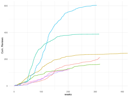
Figure 8: Cumulative weekly product reviews for randomly selected products from our subset of the Amazon dataset.

E.2 CDC ILINet influenza database

For the SIR model, we use the CDC’s ILINet database of patient visits for flu-like illnesses in the United States, broken down by Department of Health and Human Services region. Each instance in the dataset consists of weekly patient visits in a given region, over the course of one year. Each year starts in September, at the low point of the flu season. We use data from 2010 through 2019 for each of 10 regions, for 100 instances total. As the dataset only includes cumulative infections $C_{i}[t]$, rather than observations of infection and recoveries $I_{i}[t],R_{i}[t]$, we simulate these based on the dynamics (13).

Here, we take $\gamma=0.24$ as in Chowell et al. (2008), and $a$ is assumed to be 0. We take $N_{\max}$ to be the total patient population (including for non-flu illnesses) in the dataset.

E.3 COVID-19 Datasets

For observed COVID-19 cases, we use publicly available case data from the ongoing COVID-19 epidemic provided by Dong et al. (2020). We aggregate data into sub-state regions, corresponding broadly to public health service areas. The median state has seven regions. Here we take $\gamma=1/4$.

The dataset contains static demographic covariates and time-varying mobility features that affect the disease transmission rate. The dynamic covariates proxy mobility by estimating the daily fraction of people staying at home relative to a region-specific benchmark of activity in early March before social distancing measures were put in place. We also include a regional binary indicator of the days when the fraction of people staying home exceeds the benchmark by 0.2 or more.

These data are provided by Safegraph, a data company that aggregates anonymized location data from numerous applications in order to provide insights about physical places. To enhance privacy, SafeGraph excludes census block group information if fewer than five devices visited an establishment in a month from a given census block group. Documentation can be found at Saf (2020).

The static covariates capture standard demographic features of a region that influence variation in infection rates. These features fall into several categories:

• Fraction of individuals that live in close proximity or provide personal care to relatives in other generations. These covariates are reported by age group by state from survey responses conducted by UMi (2020).

• Family size from U.S. Census data, aggregated and cleaned by Cla (2020).

• Fraction of the population living in group quarters, including colleges, group homes, military quarters, and nursing homes (U.S. Census via Cla (2020)).

• Population-weighted urban status (US Census via Cla (2020))

• Prevalence of comorbidities, such as cardiovascular disease and hypertension (CDC (2020a))

• Measures of social vulnerability and poverty (U.S. Census via Cla (2020); CDC (2020b))

• Age, race and occupation distributions (U.S. Census via Cla (2020))

Appendix F Detailed description of the COVID-19 model

F.1 Approximating the arrival process with latent state

Recall the stochastic SIR process, ${(S(t),I(t),R(t)):t\geq 0}$, a multi-variate counting process determined by parameters $(N,\beta,\gamma)$. We now allow $\beta$ to be time-varying, yielding a counting process with jumps $C_{k}-C_{k-1}\sim\mathrm{Bern}\left\{\beta S_{k-1}/(\beta_{k}S_{k-1}+\gamma NI(t))\right\}$.

We obtain discrete-time diffusion processes, $\{(S_{i}[t],I_{i}[t],R_{i}[t]):t\in\mathbb{N}\}$ for instances $i\in\mathcal{I}$ by considering the Euler-approximation to the stochastic diffusion process (3) (e.g. Jacod et al. (2005)). Specifically, let $\Delta I[t]=I[t]-I[t-1]$, and define $\Delta S[t]$ and $\Delta R[t]$ analogously. A discrete-time approximation to the SIR process is then given by:

(32) $$\Delta S_{i}[t+1] =-\beta_{i}[t]({S_{i}[t]}/{N_{i}})I_{i}[t]+\nu^{S}_{i,t}$$

$$\Delta I_{i}[t+1] =\beta_{i}[t]({S_{i}[t]}/{N_{i}})I_{i}[t]-\gamma I_{i}[t]+\nu^{I}_{i,t}$$

$$\Delta R_{i}[t+1] =\gamma I_{i}[t]+\nu^{R}_{i,t}$$

where $\{\nu^{S}_{i,t}\},\{\nu^{I}_{i,t}\},\{\nu^{R}_{i,t}\}$ are appropriately defined martingale difference sequences.

In the real world, the SIR model is a latent process – we never directly observe any of the state variables $S_{i}[t],I_{i}[t],R_{i}[t]$. Instead, we observe $C_{i}[t]=I_{i}[t]+R_{i}[t]=N_{i}-S_{i}[t]$. The MLE problem for parameters $(N,\beta)$ is simply $\max_{(\beta,N)}\sum_{i,t}\log\mathbb{P}\left(C_{i}[t]|\beta,N\right)$.

This is a difficult non-linear filtering problem (and an interesting direction for research). We therefore consider an approximation: Denote by $\{(s_{i}[t],i_{i}[t],r_{i}[t]):t\in\mathbb{N}\}$ the deterministic process obtained by ignoring the martingale difference terms in the definition of the discrete time SIR process. We consider the approximation $C_{i}[t]=N_{i}-S_{i}[t]\sim(N_{i}-s_{i}[t])\omega_{i}[t]$, where $\omega_{i}[t]$ is log-normally distributed with mean $1$ and variance $\exp(\sigma^{2})-1$.

Under this approximation, we have the log likelihood function

(33) $$\log p(C_{i}[t]|N,\beta)=\left(\log C_{i}[t]-\log\left(N_{i}-s_{i}[t]\right)\right)^{2}$$

F.2 Two-Stage Estimation of the SIR model

We parameterize our estimates of $N$ as $\hat{N}_{i}(\phi,\delta)=\exp(\phi^{\top}Z_{i}+\delta_{i})P_{i}$, where $Z_{i}$ are non-time-varying, region-specific covariates, $P_{i}$ is the population of region $i$, $\phi$ is a vector of fixed effects, and $\delta_{i}\sim\mathcal{N}(0,\sigma^{2}_{\delta})$ are region-specific random effects.

Demographic and mobility factors also influence the reproduction rate of the disease. To model these effects, we estimate $\beta_{i}[t]$ as a mixed effects model incorporating covariates $\beta_{i}[t]=\exp(X_{i}[t]^{\top}\theta)+\epsilon_{i}$, where $\theta$ is a vector of fixed effects, and $\epsilon_{i}\sim\mathcal{N}(0,\sigma^{2}_{\epsilon})$ is a vector of random effects.

Given observations up to time $T$, we then estimate the model parameters $(\theta,\phi,\delta,\epsilon)$ in two stages:

1. Estimate the peak parameters $\hat{\phi},\hat{\delta}$ via MLE, for the regions $i\in Q[t]$:

   $$\hat{\phi},\hat{\delta}=\arg\max_{\phi,\delta}\left\{\max_{\theta,\epsilon}\left\{\sum_{i\in Q[t]}\sum_{t\in[T]}\log p\left(C_{i}[t]\,\big{|}\,\beta_{i}(\theta,\epsilon),\hat{N}_{i}(\phi,\delta)\right)+\log p(\epsilon,\delta)\right\}\right\}$$

   where $p$ is the likelihood defined in (33). We let $\hat{\delta}_{i}=0$ for $i\notin Q[t]$.

2. Estimate the remaining parameters over all regions $i\in\mathcal{I}$:

   (34) $$\hat{\theta},\hat{\epsilon}=\arg\max_{\theta,\epsilon}\left\{\sum_{i\in\mathcal{I}}\sum_{t\in[T]}\log p\left(C_{i}[t]\,\big{|}\,\beta_{i}(\theta,\epsilon),\hat{N}_{i}(\hat{\phi},\hat{\delta}),\right)+\log p(\epsilon,\delta)\right\}$$

We note that (34) is differentiable with respect to the parameters ($\theta,\epsilon,\phi,\delta$), and we solve it (or a weighted version) using Adam (Kingma and Ba 2014).

To identify the set $Q[t]$ of regions for which the variance of $\hat{N}$ may be small, we simply look for regions that have passed their peak rate of new infections. Concretely, we define $Q[t]$ as:

(35) $$Q[t]=\{i\in\mathcal{I}:C_{i}[t]-C_{i}[t-1]\leq\gamma_{1}\max_{\tau\leq t}\left(C_{i}[\tau]-C_{i}[\tau-1]\right)\},$$

where $\gamma_{1}\in(0,1)$ is a hyperparameter.

F.3 Performance relative to other models

To contextualize the quality of the Two-Stage model, we compare our analyzed models to the widely used IHME model ihm (2020). We note that there exist comparable models that may serve as stronger baselines; we include these results merely to demonstrate that the Two-Stage model yields high-quality predictions, comparable to widely-cited models in the literature.

Figure 9 compares state-level WMAPE for MLE, Two-Stage and IHME models, for vintages stretching back 28 days. The IHME model up to this date is, in effect, an SI model with carefully tuned parameters. We report published IHME forecasts; 10 vintages of that model were reported between April 21 and May 21. Two Stage dominates IHME across all model vintages.

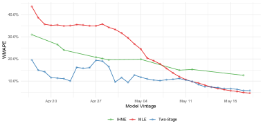
Figure 9: WMAPE for predicting state-level cumulative cases on May 21, 2020, comparing MLE and the Two-Stage approach against IHME.

References

• CDC (2020a) (2020a) CDC Interactive Atlas of Heart Disease and Stroke. https://www.cdc.gov/dhdsp/maps/atlas/index.htm.
• CDC (2020b) (2020b) CDC Social Vulnerability Index. https://svi.cdc.gov/.
• Cla (2020) (2020) Claritas. https://www.claritas.com/.
• ihm (2020) (2020) IHME. http://www.healthdata.org/sites/default/files/files/Projects/COVID/RA_COVID-forecasting-USA-EEA_042120.pdf.
• mit (2020) (2020) MIT Delphi Model. https://www.covidanalytics.io/projections.
• Saf (2020) (2020) Safegraph Social Distancing Metrics. https://docs.safegraph.com/docs/social-distancing-metrics.
• UMi (2020) (2020) University of Michigan Health and Retirement Study. https://hrs.isr.umich.edu/data-products.
• ihm (2021) (2021) Modeling covid-19 scenarios for the united states. Nature medicine 27(1):94–105.
• Anastassopoulou et al. (2020) Anastassopoulou C, Russo L, Tsakris A, Siettos C (2020) Data-based analysis, modelling and forecasting of the covid-19 outbreak. PloS one 15(3):e0230405.
• Bakshy et al. (2011) Bakshy E, Hofman JM, Mason WA, Watts DJ (2011) Everyone’s an influencer: quantifying influence on twitter. Proceedings of the fourth ACM international conference on Web search and data mining, 65–74.
• Bartlett (1949) Bartlett M (1949) Some evolutionary stochastic processes. Journal of the Royal Statistical Society. Series B (Methodological) 11(2):211–229.
• Bass (1969) Bass FM (1969) A new product growth for model consumer durables. Management science 15(5):215–227.
• Bass (2004) Bass FM (2004) Comments on “a new product growth for model consumer durables the bass model”. Management science 50(12_supplement):1833–1840.
• Bass et al. (1994) Bass FM, Krishnan TV, Jain DC (1994) Why the bass model fits without decision variables. Marketing science 13(3):203–223.
• Bendavid et al. (2021) Bendavid E, Mulaney B, Sood N, Shah S, Bromley-Dulfano R, Lai C, Weissberg Z, Saavedra-Walker R, Tedrow J, Bogan A, et al. (2021) Covid-19 antibody seroprevalence in santa clara county, california. International journal of epidemiology 50(2):410–419.
• Bertozzi et al. (2020) Bertozzi AL, Franco E, Mohler G, Short MB, Sledge D (2020) The challenges of modeling and forecasting the spread of covid-19. Proceedings of the National Academy of Sciences 117(29):16732–16738.
• Binti Hamzah et al. (2020) Binti Hamzah F, Lau C, Nazri H, Ligot D, Lee G, Tan C, et al. (2020) Coronatracker: world-wide covid-19 outbreak data analysis and prediction. Bull World Health Organ. E-pub 19.
• Biswas et al. (2020) Biswas K, Khaleque A, Sen P (2020) Covid-19 spread: Reproduction of data and prediction using a sir model on euclidean network. arXiv preprint arXiv:2003.07063 .
• Boswijk and Franses (2005) Boswijk HP, Franses PH (2005) On the econometrics of the bass diffusion model. Journal of Business & Economic Statistics 23(3):255–268.
• Calafiore et al. (2020) Calafiore GC, Novara C, Possieri C (2020) A modified sir model for the covid-19 contagion in italy. 2020 59th IEEE Conference on Decision and Control (CDC), 3889–3894 (IEEE).
• Castro et al. (2020) Castro M, Ares S, Cuesta JA, Manrubia S (2020) The turning point and end of an expanding epidemic cannot be precisely forecast. Proceedings of the National Academy of Sciences 117(42):26190–26196.
• Chikina and Pegden (2020) Chikina M, Pegden W (2020) Modeling strict age-targeted mitigation strategies for covid-19. PloS one 15(7):e0236237.
• Chowell et al. (2008) Chowell G, Miller M, Viboud C (2008) Seasonal influenza in the united states, france, and australia: transmission and prospects for control. Epidemiology & Infection 136(6):852–864.
• Cramér et al. (1946) Cramér H, et al. (1946) Mathematical methods of statistics. Mathematical methods of statistics. .
• Darling et al. (2008) Darling R, Norris JR, et al. (2008) Differential equation approximations for markov chains. Probability surveys 5:37–79.
• Del Valle et al. (2007) Del Valle S, Hyman J, Hethcote H, Eubank S (2007) Mixing patterns between age groups in social networks. Social Networks 29(4):539–554, ISSN 0378-8733, URL http://dx.doi.org/https://doi.org/10.1016/j.socnet.2007.04.005.
• Del Valle et al. (2013) Del Valle SY, Hyman JM, Chitnis N (2013) Mathematical models of contact patterns between age groups for predicting the spread of infectious diseases. Math. Biosci. Eng. 10(5-6):1475–1497.
• Dong et al. (2020) Dong E, Du H, Gardner L (2020) An interactive web-based dashboard to track covid-19 in real time. The Lancet infectious diseases 20(5):533–534.
• Duffy et al. (2012) Duffy KR, Wellard CJ, Markham JF, Zhou JH, Holmberg R, Hawkins ED, Hasbold J, Dowling MR, Hodgkin PD (2012) Activation-induced b cell fates are selected by intracellular stochastic competition. Science 335(6066):338–341.
• Eldar (2008) Eldar YC (2008) Rethinking biased estimation: Improving maximum likelihood and the Cramér-Rao bound (Now Publishers Inc).
• Evans et al. (2005) Evans ND, White LJ, Chapman MJ, Godfrey KR, Chappell MJ (2005) The structural identifiability of the susceptible infected recovered model with seasonal forcing. Mathematical biosciences 194(2):175–197.
• Gaeta (2020) Gaeta G (2020) A simple sir model with a large set of asymptomatic infectives. arXiv preprint arXiv:2003.08720 .
• Giordano et al. (2020) Giordano G, Blanchini F, Bruno R, Colaneri P, Di Filippo A, Di Matteo A, Colaneri M (2020) Modelling the covid-19 epidemic and implementation of population-wide interventions in italy. Nature Medicine 1–6.
• Goel and Sharma (2020) Goel R, Sharma R (2020) Mobility based sir model for pandemics-with case study of covid-19. 2020 IEEE/ACM International Conference on Advances in Social Networks Analysis and Mining (ASONAM), 110–117 (IEEE).
• Hardie et al. (1998) Hardie BG, Fader PS, Wisniewski M (1998) An empirical comparison of new product trial forecasting models. Journal of Forecasting 17(3-4):209–229.
• Hauser et al. (2006) Hauser J, Tellis GJ, Griffin A (2006) Research on innovation: A review and agenda for marketing science. Marketing science 25(6):687–717.
• Havers et al. (2020) Havers FP, Reed C, Lim T, Montgomery JM, Klena JD, Hall AJ, Fry AM, Cannon DL, Chiang CF, Gibbons A, et al. (2020) Seroprevalence of antibodies to sars-cov-2 in 10 sites in the united states, march 23-may 12, 2020. JAMA internal medicine 180(12):1576–1586.
• Hawkins et al. (2007) Hawkins ED, Turner ML, Dowling MR, Van Gend C, Hodgkin PD (2007) A model of immune regulation as a consequence of randomized lymphocyte division and death times. Proceedings of the National Academy of Sciences 104(12):5032–5037.
• Ivorra et al. (2020) Ivorra B, Ferrández MR, Vela-Pérez M, Ramos AM (2020) Mathematical modeling of the spread of the coronavirus disease 2019 (covid-19) taking into account the undetected infections. the case of china. Communications in nonlinear science and numerical simulation 88:105303.
• Jacod et al. (2005) Jacod J, Kurtz TG, Méléard S, Protter P (2005) The approximate euler method for lévy driven stochastic differential equations. Annales de l’IHP Probabilités et statistiques, volume 41, 523–558.
• Jain and Rao (1990) Jain DC, Rao RC (1990) Effect of price on the demand for durables: Modeling, estimation, and findings. Journal of Business & Economic Statistics 8(2):163–170.
• Janson (2018) Janson S (2018) Tail bounds for sums of geometric and exponential variables. Statistics & Probability Letters 135:1–6.
• Kermack and McKendrick (1927) Kermack WO, McKendrick AG (1927) A contribution to the mathematical theory of epidemics. Proceedings of the royal society of london. Series A, Containing papers of a mathematical and physical character 115(772):700–721.
• Kingma and Ba (2014) Kingma DP, Ba J (2014) Adam: A method for stochastic optimization. arXiv preprint arXiv:1412.6980 .
• Kucharski et al. (2020) Kucharski AJ, Russell TW, Diamond C, Liu Y, Edmunds J, Funk S, Eggo RM, Sun F, Jit M, Munday JD, et al. (2020) Early dynamics of transmission and control of covid-19: a mathematical modelling study. The lancet infectious diseases .
• Lau et al. (2021) Lau H, Khosrawipour T, Kocbach P, Ichii H, Bania J, Khosrawipour V (2021) Evaluating the massive underreporting and undertesting of covid-19 cases in multiple global epicenters. Pulmonology 27(2):110–115.
• Lee et al. (2014) Lee H, Kim SG, Park Hw, Kang P (2014) Pre-launch new product demand forecasting using the bass model: A statistical and machine learning-based approach. Technological Forecasting and Social Change 86:49–64.
• Li et al. (2020) Li R, Pei S, Chen B, Song Y, Zhang T, Yang W, Shaman J (2020) Substantial undocumented infection facilitates the rapid dissemination of novel coronavirus (sars-cov-2). Science 368(6490):489–493.
• Mahajan et al. (1995) Mahajan V, Muller E, Bass FM (1995) Diffusion of new products: Empirical generalizations and managerial uses. Marketing science 14(3_supplement):G79–G88.
• Mahajan et al. (2000) Mahajan V, Muller E, Wind Y (2000) New-product diffusion models, volume 11 (Springer Science & Business Media).
• Massonnaud et al. (2020) Massonnaud C, Roux J, Crépey P (2020) Covid-19: Forecasting short term hospital needs in france. medRxiv .
• Meyn and Tweedie (2012) Meyn SP, Tweedie RL (2012) Markov chains and stochastic stability (Springer Science & Business Media).
• Miller (2012) Miller JC (2012) A note on the derivation of epidemic final sizes. Bulletin of mathematical biology 74(9):2125–2141.
• Miller (2017) Miller JC (2017) Mathematical models of sir disease spread with combined non-sexual and sexual transmission routes. Infectious Disease Modelling 2(1):35–55.
• Moein et al. (2021) Moein S, Nickaeen N, Roointan A, Borhani N, Heidary Z, Javanmard SH, Ghaisari J, Gheisari Y (2021) Inefficiency of sir models in forecasting covid-19 epidemic: a case study of isfahan. Scientific reports 11(1):4725.
• Ni et al. (2019) Ni J, Li J, McAuley J (2019) Justifying recommendations using distantly-labeled reviews and fine-grained aspects. Proceedings of the 2019 Conference on Empirical Methods in Natural Language Processing and the 9th International Joint Conference on Natural Language Processing (EMNLP-IJCNLP), 188–197.
• Peterson and Mahajan (1978) Peterson RA, Mahajan V (1978) Multi-product growth models. Research in marketing 1(20):1–23.
• Pullano et al. (2021) Pullano G, Di Domenico L, Sabbatini CE, Valdano E, Turbelin C, Debin M, Guerrisi C, Kengne-Kuetche C, Souty C, Hanslik T, et al. (2021) Underdetection of cases of covid-19 in france threatens epidemic control. Nature 590(7844):134–139.
• Roosa and Chowell (2019) Roosa K, Chowell G (2019) Assessing parameter identifiability in compartmental dynamic models using a computational approach: application to infectious disease transmission models. Theoretical Biology and Medical Modelling 16(1):1.
• Srinivasan and Mason (1986) Srinivasan V, Mason CH (1986) Nonlinear least squares estimation of new product diffusion models. Marketing science 5(2):169–178.
• Sultan et al. (1990) Sultan F, Farley JU, Lehmann DR (1990) A meta-analysis of applications of diffusion models. Journal of marketing research 27(1):70–77.
• Van den Bulte and Joshi (2007) Van den Bulte C, Joshi YV (2007) New product diffusion with influentials and imitators. Marketing science 26(3):400–421.
• Van den Bulte and Lilien (1997) Van den Bulte C, Lilien GL (1997) Bias and systematic change in the parameter estimates of macro-level diffusion models. Marketing Science 16(4):338–353.
• Weiss (2013) Weiss HH (2013) The sir model and the foundations of public health. Materials matematics 0001–17.
• Wormald (1995) Wormald NC (1995) Differential equations for random processes and random graphs. The annals of applied probability 1217–1235.
• Wu et al. (2020) Wu JT, Leung K, Leung GM (2020) Nowcasting and forecasting the potential domestic and international spread of the 2019-ncov outbreak originating in wuhan, china: a modelling study. The Lancet 395(10225):689–697.
• Zegers (2015) Zegers P (2015) Fisher information properties. Entropy 17(7):4918–4939.