Quantum gravitational interaction between two objects induced by external gravitational radiation fields

Abstract

We explore, in the framework of linearized quantum gravity, the induced gravitational interaction between two gravitationally polarizable objects in their ground states in the presence of an external quantized gravitational radiation field. The interaction energy decreases as $r^{-5}$ in the near regime, and oscillates with a decreasing amplitude proportional to $r^{-1}$ in the far regime, where $r$ is the distance between the two objects. The interaction can be either attractive or repulsive depending on the propagation direction, polarization and frequency of the external gravitational field. That is, the induced interaction can be manipulated by varying the relative direction between the orientation of the objects with respect to the propagation direction of the incident gravitational radiation.

I Introduction

It is well known that in a quantum sense, there inevitably exist quantum vacuum fluctuations, which may induce some novel effects. One of the most famous examples is the electromagnetic Casimir-Polder (CP) interaction CP . In general, fluctuating electromagnetic fields in vacuum induce instantaneous electric dipole moments in neutral atoms, which then couple with each other via the exchange of virtual photons to yield an interaction energy. For atoms or molecules in different states, such CP interactions behave differently in terms of distance-dependence PT ; Salam ; Power1993pra ; McLone1965 ; Gomberoff1966 ; Power1993Chem ; Power1995 ; Rizzuto2004 ; Sherkunov2007 ; Preto2013 ; Donaire2015 ; Milonni2015 ; Berman2015 ; Jentschura2017 . For example, the interatomic or intermolecular interaction behaves as $r^{-6}$ and $r^{-7}$ in the near and far regimes respectively when the atoms or molecules are in their ground states CP , while it behaves as $r^{-3}$ and $r^{-1}$ in the near and far regimes respectively when they are prepared in a symmetric/antisymmetric entangled state PT .

Likewise, one may also expect a gravitational CP-like interaction if one accepts that basic quantum principles are also applicable to gravity. Unfortunately, a full theory of quantum gravity is elusive at present. Even though, one may still study quantum gravitational effects at low energies in the framework of linearized quantum gravity yu1999 ; Ford1995 , the basic idea of which is to express the spacetime metric as a sum of the flat background spacetime metric and a linearized perturbation, and quantize the perturbation part in the canonical approach. Based on linearized quantum gravity, the gravitational CP-like interactions between two gravitationally polarizable objects in their ground states, and between one gravitationally polarizable object and a gravitational boundary, have recently been studied in Refs. Ford2016 ; Wu2016 ; Wu2017 ; Holstein2017 ; Hu2017 ; yu2018 . Similar to the electromagnetic case, the behaviors of gravitational CP-like interactions are significantly different when the gravitationally polarizable objects are prepared in different states. For example, the gravitational CP-like potential is found to be proportional to $r^{-10}$ and $r^{-11}$ in the near and far regimes respectively when the two objects are in their ground states Ford2016 ; Wu2016 ; Wu2017 ; Holstein2017 , while it behaves as $r^{-5}$ and $r^{-1}$ in the near and far regimes respectively when the two objects are in a symmetric/antisymmetric entangled state Hu2019 .

Naturally, a question arises as to whether such quantum gravitational effects can be modified or enhanced in certain circumstances. Fortunately, there are similar examples in quantum electrodynamics. For example, the interaction between two ground-state atoms or molecules is found to be modified in the presence of external electromagnetic radiation fields Thirunamachandran1980 ; Milonni1992 ; Milonni1996 ; Salam2006 ; Salam2007 . That is, the externally applied electromagnetic field induces dipole moments in atoms or molecules, which are coupled with each other via the exchange of a single virtual photon, and an interaction is induced. This process is clearly different from the case without external electromagnetic fields, which arises from two-photon exchange. Similarly, in the gravitational case, one may expect that the quantum gravitational quadrupole-quadrupole interactions will also be modified in the presence of an external gravitational radiation field.

In this paper, we explore the quantum gravitational quadrupole-quadrupole interaction between a pair of gravitationally polarizable objects in their ground states, which are subjected to a weak external gravitational radiation field based on the leading-order perturbation theory in the framework of linearized quantum gravity. First, we describe in details the system we deal with. Then, we obtain the general expression for the interaction energy between the two objects. Finally, we discuss our results in specific cases and obtain the corresponding interaction potentials. Throughout this paper, the Einstein summation convention for repeated indices is assumed, and the Latin indices run from $1$ to $3$ while the Greek indices run from $0$ to $3$. Units with $\hbar=c=16\pi G=1$ are applied, where $\hbar$ is the reduced Planck constant, $c$ is the speed of light and $G$ is the Newtonian gravitational constant.

II Basic equations

We consider two gravitationally polarizable objects (labeled as A and B) coupled with a bath of fluctuating gravitational fields in vacuum, which are subjected to a weak external gravitational radiation field. The objects A and B are modeled as two-level systems with two internal energy levels, $\pm\frac{1}{2}\omega_{0}$, associated with the eigenstates $|g\rangle$ and $|e\rangle$, respectively. The total Hamiltonian is

$$H=H_{F}+H_{R}+H_{S}+H_{I},$$ (1)

where $H_{F}$ is the Hamiltonian of the fluctuating vacuum gravitational field, $H_{R}$ the Hamiltonian of the external gravitational radiation field, $H_{S}$ the Hamiltonian of the two-level systems (A and B), and $H_{I}$ the interaction Hamiltonian between the objects and the gravitational fields. Here $H_{I}$ takes the form

$$H_{I}=-\frac{1}{2}Q^{A}_{ij}[\epsilon_{ij}(\vec{x}_{A})+E_{ij}(\vec{x}_{A})]-\frac{1}{2}Q^{B}_{ij}[\epsilon_{ij}(\vec{x}_{B})+E_{ij}(\vec{x}_{B})],$$ (2)

where $Q^{A(B)}_{ij}$ is the induced quadrupole moment of the object A (B), $\epsilon_{ij}$ is the gravitoelectric tensor characterizing the weak external gravitational radiation field, and $E_{ij}$ is the gravitoelectric tensor of the fluctuating vacuum gravitational fields defined as $E_{ij}=C_{0i0j}$ by an analogy between the linearized Einstein field equations and the Maxwell equations WB , where $C_{\mu\nu\alpha\beta}$ is the Weyl tensor. We write the spacetime metric $g_{\mu\nu}$ as a sum of the flat spacetime metric $\eta_{\mu\nu}$ and a linearized perturbation $h_{\mu\nu}$, then the gravitoelectric tensor $E_{ij}$ can be expressed as (in the transverse traceless gauge)

$$E_{ij}=\frac{1}{2}\ddot{h}_{ij}.$$ (3)

Suppose that the linearized perturbation $h_{\mu\nu}$ is quantized, in this regard, we can decompose $h_{\mu\nu}$ into positive and negative frequency parts $h_{\mu\nu}^{+}$ and $h_{\mu\nu}^{-}$, respectively, and define the gravitational vacuum state $|0\rangle$ as

$$h_{\mu\nu}^{+}|0\rangle=0,\quad\langle 0|h_{\mu\nu}^{-}=0.$$ (4)

It follows immediately that $\langle 0|h_{\mu\nu}|0\rangle=0$. In general, however, $\langle 0|(h_{\mu\nu})^{2}|0\rangle\neq 0$, where the expectation value is understood to be suitably renormalized. In the transverse traceless gauge, the quantized gravitational perturbations have only spatial components $h_{ij}$, which takes the standard form

$$h_{ij}=\sum_{\vec{p},\lambda}\sqrt{\frac{1}{2\omega(2\pi)^{3}}}\left[a_{\lambda}(\vec{p})e^{(\lambda)}_{ij}e^{i(\vec{p}\cdot\vec{x}-\omega t)}+\text{H.c.}\right],$$ (5)

where $a_{\lambda}(\vec{p})$ is the annihilation operator of the gravitational vacuum field with wave vector $\vec{p}$ and polarization $\lambda$, $e^{(\lambda)}_{ij}$ are polarization tensors, $\omega=|\vec{p}|=(p_{x}^{2}+p_{y}^{2}+p_{z}^{2})^{1/2}$, and H.c. denotes the Hermitian conjugate. As for the weak external gravitational radiation field, we assume that it can be described as a quantized monochromatic gravitational wave containing $N$ gravitons. Then, the corresponding gravitoelectric tensor $\epsilon_{ij}$ can be given as

$$\epsilon_{ij}=-\frac{1}{2}\sqrt{\frac{\omega_{R}^{3}\rho_{n}}{2N(2\pi)^{3}}}\left[b(\vec{k})e_{ij}^{(\varepsilon)}e^{i(\vec{k}\cdot\vec{x}-\omega_{R}t)}+H.c.\right],$$ (6)

where $\rho_{n}$ is the number density of gravitons, $b(\vec{k})$ and $e_{ij}^{(\varepsilon)}$ are respectively the corresponding annihilation operator and the polarization tensors with $|\vec{k}|=\omega_{R}$, and $\varepsilon$ labels the polarization state.

In the absence of an external gravitational field, the interaction between a pair of ground-state objects coupled with a bath of fluctuating gravitational fields in vacuum is a fourth-order effect Ford2016 ; Wu2016 ; Wu2017 : The gravitational vacuum fluctuations induce quadrupole moments in the two objects, which are correlated and an interaction energy is thus induced. Physically speaking, such an induced interaction originates from vacuum fluctuations and arises through the exchange of a pair of virtual gravitons between the two objects. In the present case, the leading interaction between quadrupole moments induced by the external gravitational radiation field will also be a fourth-order effect. However, the difference is that the quadrupole moments are now induced by the external gravitational field, which are then correlated to each other through gravitational vacuum fluctuations. That is, a real graviton will be scattered by a pair of objects which are coupled via the exchange of a virtual graviton, and an interaction is then induced, which is analogous to the electromagnetic case Thirunamachandran1980 .

We choose the initial state of the system to be

$$|\phi\rangle=|g_{A}g_{B}\rangle|0\rangle|N\rangle,$$ (7)

where $|g_{A}g_{B}\rangle$ is the ground state of the objects, $|0\rangle$ is the vacuum state of the fluctuating gravitational field, and $|N\rangle$ is the number state of the external gravitational radiation field. The initial energy of the whole system is $E_{\phi}=E_{0}+N\omega_{R}$, where $E_{0}$ denotes the ground-state energy of the objects and fluctuating gravitational field in vacuum. The leading contribution to the interaction energy can be obtained from fourth-order perturbation theory, which contains $48$ possible Feynman diagrams in our case, and a typical one is shown in Fig. 1.

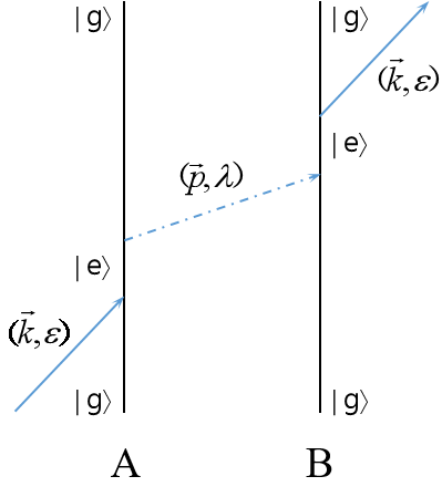
Figure 1: A typical time-ordered diagram for the calculation of inter-object interaction in the existence of an external quantized gravitational field. The blue solid line represents a real graviton, while the dotted one represents a virtual one.

However, the calculations can be greatly simplified by collapsing the two one-graviton interaction vertices in the time-ordered diagrams, which can be described as an effective two-graviton interaction Hamiltonian. To do this, we introduce the gravitational polarizability of the objects, and, for simplicity, assume that the objects are isotropically polarizable. Then, the induced quadrupole can be expressed as

$$Q^{A(B)}_{ij}=\alpha^{(\varepsilon)}_{A(B)}\epsilon_{ij},$$ (8)

where $\alpha^{(\varepsilon)}_{A(B)}$ is the isotropic polarizability of object A(B). In order to calculate the interaction, we only keep the corresponding terms after substituting Eq. (8) into Eq. (2). Then, the effective Hamiltonian takes the form

$$H^{eff}_{I}=-\frac{1}{2}\alpha^{(\varepsilon)}_{A}\epsilon_{ij}(\vec{x}_{A})E_{ij}(\vec{x}_{A})-\frac{1}{2}\alpha^{(\varepsilon)}_{B}\epsilon_{ij}(\vec{x}_{B})E_{ij}(\vec{x}_{B}).$$ (9)

The interaction energy can be calculated based on the second order perturbation theory

$$\Delta E=-\sum_{I}\frac{\langle\phi|H^{eff}_{I}|I\rangle\langle I|H^{eff}_{I}|\phi\rangle}{E_{I}-E_{\phi}},$$ (10)

with only four contributing time-ordered diagrams as shown in Fig. 2.

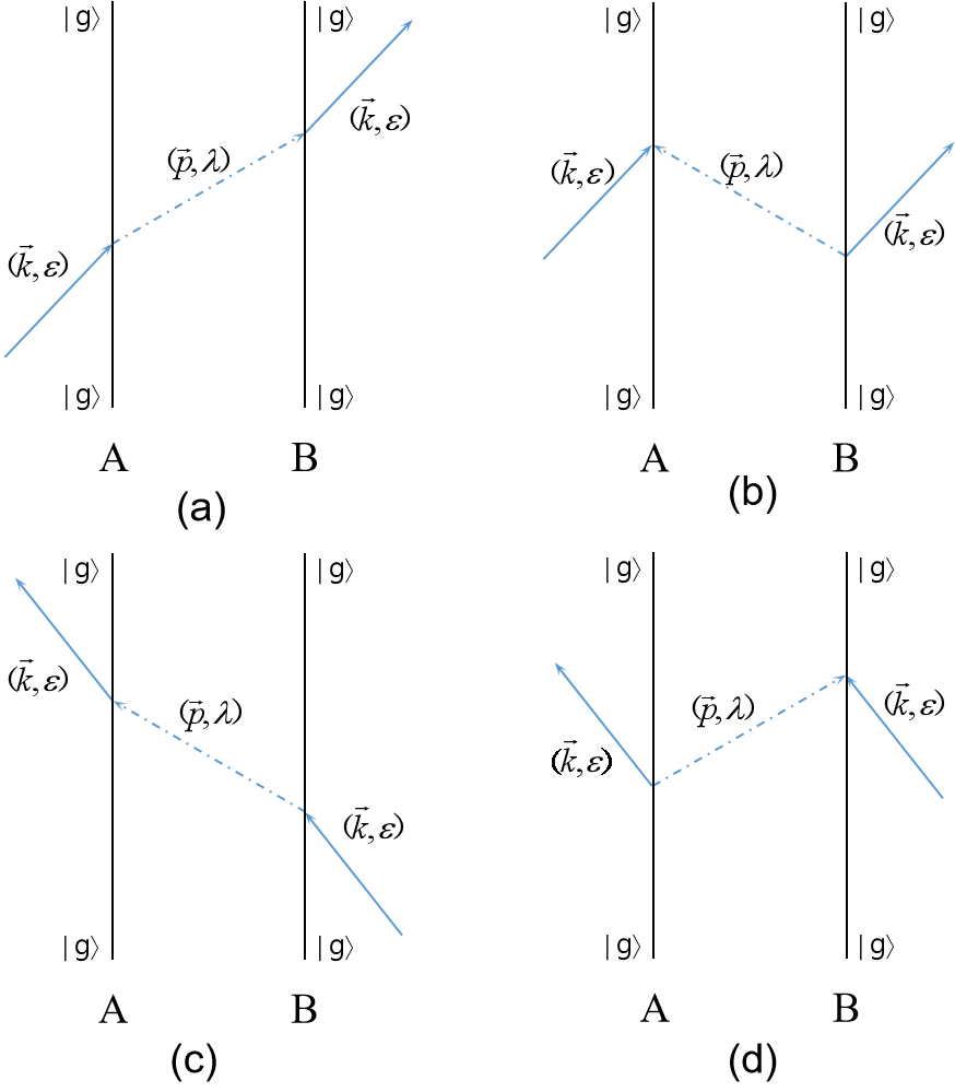
Figure 2: Four time-ordered diagrams represent the four contributing terms in the second order perturbation theory.

Summing up all the contributions, the interaction energy can be expressed as

$$\Delta E_{AB} = -\frac{\omega^{3}_{R}\rho_{n}}{256(2\pi)^{6}}\alpha^{(\varepsilon)}_{A}\alpha^{(\varepsilon)}_{B}e^{(\varepsilon)}_{ij}e^{(\varepsilon)}_{kl}\cos{(\vec{k}\cdot\vec{r})}\int d^{3}\vec{p}\sum_{\lambda}e^{(\lambda)}_{ij}e^{(\lambda)}_{kl}\frac{\omega^{3}}{\omega-\omega_{R}}e^{i\vec{p}\cdot\vec{r}}$$ (11)

$$- \frac{(N+1)\omega^{3}_{R}\rho_{n}}{256N(2\pi)^{6}}\alpha^{(\varepsilon)}_{A}\alpha^{(\varepsilon)}_{B}e^{(\varepsilon)}_{ij}e^{(\varepsilon)}_{kl}\cos{(\vec{k}\cdot\vec{r})}\int d^{3}\vec{p}\sum_{\lambda}e^{(\lambda)}_{ij}e^{(\lambda)}_{kl}\frac{\omega^{3}}{\omega+\omega_{R}}e^{i\vec{p}\cdot\vec{r}},$$

where $\vec{r}=\vec{x}_{A}-\vec{x}_{B}$. Here the summation of polarization tensors in the transverse traceless gauge gives yu1999

$$\sum_{\lambda}e^{(\lambda)}_{ij}e^{(\lambda)}_{kl}=\delta_{ik}\delta_{jl}+\delta_{il}\delta_{jk}-\delta_{ij}\delta_{kl}-\frac{1}{\omega^{2}}H_{ijkl}+\frac{1}{\omega^{4}}P_{ijkl},$$

where

$$H_{ijkl}=\partial_{i}\partial_{j}\delta_{kl}+\partial_{k}\partial_{l}\delta_{ij}-\partial_{i}\partial_{k}\delta_{jl}-\partial_{i}\partial_{l}\delta_{jk}-\partial_{j}\partial_{k}\delta_{il}-\partial_{j}\partial_{l}\delta_{ik},\ P_{ijkl}=\partial_{i}\partial_{j}\partial_{k}\partial_{l}.$$ (12)

For convenience, we define a gravitational radiation intensity $I_{R}$ in analogy to the electromagnetic case Buhmann2019 as

$$I_{R}=\langle N|\epsilon^{2}_{ij}|N\rangle=\frac{\omega^{3}_{R}\rho_{n}}{8N(2\pi)^{3}}(2N+1),$$ (13)

since the intensity of the radiation field should be proportional to the number of gravitons. For a large graviton number $N\gg 1$, we have

$$I_{R}\simeq\frac{\omega^{3}_{R}\rho_{n}}{4(2\pi)^{3}}.$$ (14)

Thus, the interaction energy (11) can be expressed as

$$\Delta E_{AB}=-\frac{I_{R}}{128\pi}\alpha^{(\varepsilon)}_{A}\alpha^{(\varepsilon)}_{B}e^{(\varepsilon)}_{ij}e^{(\varepsilon)}_{kl}\cos{(\vec{k}\cdot\vec{r})}V_{ijkl},$$ (15)

where

$$V_{ijkl}=\left[(\delta_{ik}\delta_{jl}+\delta_{il}\delta_{jk}-\delta_{ij}\delta_{kl})\omega^{4}_{R}-\omega^{2}_{R}H_{ijkl}+P_{ijkl}\right]\frac{\cos{\omega_{R}r}}{r}.$$ (16)

After some algebraic manipulations, the full form of $V_{ijkl}$ is given by

$$V_{ijkl}=\frac{1}{r^{5}}\bigg{[} (\delta_{ik}\delta_{jl}+\delta_{il}\delta_{jk}-\delta_{ij}\delta_{kl}+\hat{r}_{i}\hat{r}_{j}\delta_{kl}+\hat{r}_{k}\hat{r}_{l}\delta_{ij}-\hat{r}_{i}\hat{r}_{k}\delta_{jl}$$ (17)

$$-\hat{r}_{i}\hat{r}_{l}\delta_{jk}-\hat{r}_{j}\hat{r}_{k}\delta_{il}-\hat{r}_{j}\hat{r}_{l}\delta_{ik}+\hat{r}_{i}\hat{r}_{j}\hat{r}_{k}\hat{r}_{l})r^{4}\omega^{4}_{R}\cos{\omega_{R}r}$$

$$+2(-\delta_{ik}\delta_{jl}-\delta_{il}\delta_{jk}+\delta_{ij}\delta_{kl}-\hat{r}_{i}\hat{r}_{j}\delta_{kl}-\hat{r}_{k}\hat{r}_{l}\delta_{ij}+2\hat{r}_{j}\hat{r}_{k}\delta_{il}$$

$$+2\hat{r}_{j}\hat{r}_{l}\delta_{ik}+2\hat{r}_{i}\hat{r}_{k}\delta_{jl}+2\hat{r}_{i}\hat{r}_{l}\delta_{jk}-5\hat{r}_{i}\hat{r}_{j}\hat{r}_{k}\hat{r}_{l})r^{3}\omega^{3}_{R}\sin{\omega_{R}r}$$

$$+(-3\delta_{ik}\delta_{jl}-3\delta_{il}\delta_{jk}+\delta_{ij}\delta_{kl}+3\hat{r}_{i}\hat{r}_{j}\delta_{kl}+3\hat{r}_{k}\hat{r}_{l}\delta_{ij}+9\hat{r}_{j}\hat{r}_{k}\delta_{il}$$

$$+9\hat{r}_{j}\hat{r}_{l}\delta_{ik}+9\hat{r}_{i}\hat{r}_{k}\delta_{jl}+9\hat{r}_{i}\hat{r}_{l}\delta_{jk}-45\hat{r}_{i}\hat{r}_{j}\hat{r}_{k}\hat{r}_{l})r^{2}\omega^{2}_{R}\cos{\omega_{R}r}$$

$$+3(\delta_{ik}\delta_{jl}+\delta_{il}\delta_{jk}+\delta_{ij}\delta_{kl}-5\hat{r}_{i}\hat{r}_{j}\delta_{kl}-5\hat{r}_{k}\hat{r}_{l}\delta_{ij}-5\hat{r}_{j}\hat{r}_{k}\delta_{il}$$

$$-5\hat{r}_{j}\hat{r}_{l}\delta_{ik}-5\hat{r}_{i}\hat{r}_{k}\delta_{jl}-5\hat{r}_{i}\hat{r}_{l}\delta_{jk}+35\hat{r}_{i}\hat{r}_{j}\hat{r}_{k}\hat{r}_{l})r\omega_{R}\sin{\omega_{R}r}$$

$$+3(\delta_{ik}\delta_{jl}+\delta_{il}\delta_{jk}+\delta_{ij}\delta_{kl}-5\hat{r}_{i}\hat{r}_{j}\delta_{kl}-5\hat{r}_{k}\hat{r}_{l}\delta_{ij}-5\hat{r}_{j}\hat{r}_{k}\delta_{il}$$

$$-5\hat{r}_{j}\hat{r}_{l}\delta_{ik}-5\hat{r}_{i}\hat{r}_{k}\delta_{jl}-5\hat{r}_{i}\hat{r}_{l}\delta_{jk}+35\hat{r}_{i}\hat{r}_{j}\hat{r}_{k}\hat{r}_{l})\cos{\omega_{R}r}\bigg{]},$$

where $\hat{r}_{i}$ is a component of the unit vector $\vec{r}/r$. The above result shows that the total interaction energy depends on the polarization, frequency and propagation direction of the external gravitational radiation field. In the following, we consider two explicit examples.

First, when the propagation direction of the external gravitational radiation field is parallel to the orientation of the two objects, or equivalently, the polarization plane is perpendicular to $\vec{r}$ , i.e., $\vec{k}\cdot\vec{r}=\omega_{R}r$ and $e^{(\varepsilon)}_{ij}\hat{r}_{i}=0$, Eq. (15) can be rewritten as

$$\Delta E_{AB}=-\frac{I_{R}}{64\pi r^{5}}\alpha^{(\varepsilon)}_{A}\alpha^{(\varepsilon)}_{B}e^{(\varepsilon)}_{ij}e^{(\varepsilon)}_{ij} \Big{(}r^{4}\omega^{4}_{R}\cos^{2}{\omega_{R}r}-2r^{3}\omega^{3}_{R}\sin{\omega_{R}r}\cos{\omega_{R}r}-3r^{2}\omega^{2}_{R}\cos^{2}{\omega_{R}r}$$ (18)

$$+3r\omega_{R}\sin{\omega_{R}r}\cos{\omega_{R}r}+3\cos^{2}{\omega_{R}r}\Big{)},$$

where $e^{(\varepsilon)}_{ii}=0$ and $e^{(\varepsilon)}_{ij}=e^{(\varepsilon)}_{ji}$ have been applied. In the near regime, i.e., $\omega_{R}r\ll 1$, the leading term takes the form

$$\Delta E_{AB}\simeq-\frac{3I_{R}}{64\pi r^{5}}\alpha^{(\varepsilon)}_{A}\alpha^{(\varepsilon)}_{B}e^{(\varepsilon)}_{ij}e^{(\varepsilon)}_{ij},$$ (19)

while in the far regime, i.e., $\omega_{R}r\gg 1$, it becomes

$$\Delta E_{AB}\simeq-\frac{\omega^{4}_{R}I_{R}}{64\pi r}\alpha^{(\varepsilon)}_{A}\alpha^{(\varepsilon)}_{B}e^{(\varepsilon)}_{ij}e^{(\varepsilon)}_{ij}\cos{(\omega_{R}r+\phi)}\cos{\omega_{R}r},$$ (20)

where $\phi=\arcsin{\frac{2}{\sqrt{4+\omega_{R}^{2}r^{2}}}}$. This shows that the gravitational interaction between two objects in the presence of an external gravitational field decreases as $r^{-5}$ in the near regime, while in the far regime it oscillates with a decreasing amplitude proportional to $r^{-1}$. Moreover, from Eqs. (19)-(20), we observe that in the near regime, the interaction is always attractive, while in the far regime, it can be attractive or repulsive depending on the frequency of the external gravitational field and the interobject distance.

Second, if the propagation direction of the incident external gravitational radiation field is perpendicular to the orientation of the two objects, i.e., $\vec{k}\cdot\vec{r}=0$, then Eq. (15) yields

$$\Delta E_{AB}=-\frac{I_{R}}{128\pi r^{5}}\alpha^{(\varepsilon)}_{A}\alpha^{(\varepsilon)}_{B} \Big{[}\left(2e^{(\varepsilon)}_{ij}e^{(\varepsilon)}_{ij}-4e^{(\varepsilon)}_{i1}e^{(\varepsilon)}_{i1}+e^{(\varepsilon)}_{11}e^{(\varepsilon)}_{11}\right)r^{4}\omega^{4}_{R}\cos{\omega_{R}r}$$ (21)

$$+2\left(-2e^{(\varepsilon)}_{ij}e^{(\varepsilon)}_{ij}+8e^{(\varepsilon)}_{i1}e^{(\varepsilon)}_{i1}-5e^{(\varepsilon)}_{11}e^{(\varepsilon)}_{11}\right)r^{3}\omega^{3}_{R}\sin{\omega_{R}r}$$

$$+3\left(-2e^{(\varepsilon)}_{ij}e^{(\varepsilon)}_{ij}+12e^{(\varepsilon)}_{i1}e^{(\varepsilon)}_{i1}-15e^{(\varepsilon)}_{11}e^{(\varepsilon)}_{11}\right)r^{2}\omega^{2}_{R}\cos{\omega_{R}r}$$

$$+3\left(2e^{(\varepsilon)}_{ij}e^{(\varepsilon)}_{ij}-20e^{(\varepsilon)}_{i1}e^{(\varepsilon)}_{i1}+35e^{(\varepsilon)}_{11}e^{(\varepsilon)}_{11}\right)r\omega_{R}\sin{\omega_{R}r}$$

$$+3\left(2e^{(\varepsilon)}_{ij}e^{(\varepsilon)}_{ij}-20e^{(\varepsilon)}_{i1}e^{(\varepsilon)}_{i1}+35e^{(\varepsilon)}_{11}e^{(\varepsilon)}_{11}\right)\cos{\omega_{R}r}\Big{]},$$

where we have taken $\hat{r}_{i}=(1,0,0)$ and $\vec{k}=(0,0,k)$. In the near regime, i.e., $\omega_{R}r\ll 1$, the leading term of Eq. (21) becomes

$$\Delta E_{AB}\simeq-\frac{3I_{R}}{128\pi r^{5}}\alpha^{(\varepsilon)}_{A}\alpha^{(\varepsilon)}_{B}\left(2e^{(\varepsilon)}_{ij}e^{(\varepsilon)}_{ij}-20e^{(\varepsilon)}_{i1}e^{(\varepsilon)}_{i1}+35e^{(\varepsilon)}_{11}e^{(\varepsilon)}_{11}\right).$$ (22)

So, the interaction energy decreases as $r^{-5}$ in the near regime. Remarkably, it can be either attractive or repulsive depending on the polarization of the external gravitational radiation field. For example, the interaction is attractive if the polarization tensor contains only diagonal elements which may correspond to the $+$ mode of gravitational waves, while it behaves as repulsive when there are only off-diagonal elements which may correspond to the $\times$ mode. In the far regime, i.e., $\omega_{R}r\gg 1$, Eq. (21) reduces to

$$\Delta E_{AB}\simeq-\frac{\omega^{4}_{R}I_{R}}{128\pi r}\alpha^{(\varepsilon)}_{A}\alpha^{(\varepsilon)}_{B}\left(2e^{(\varepsilon)}_{ij}e^{(\varepsilon)}_{ij}-4e^{(\varepsilon)}_{i1}e^{(\varepsilon)}_{i1}+e^{(\varepsilon)}_{11}e^{(\varepsilon)}_{11}\right)\cos{\omega_{R}r}.$$ (23)

That is, when the propagation direction of external gravitational radiation field is perpendicular to the orientation of the objects, the interaction energy in the far regime oscillates with a decreasing amplitude which is proportional to $r^{-1}$. The interaction can be attractive or repulsive depending on the polarization and frequency of the external gravitational radiation field, and the interobject distance. For a given external field, the interaction periodically behaves between attractive and repulsive as the interobject distance varies.

III Discussion

In this paper, we investigate the gravitational quadrupole-quadrupole interaction between two gravitationally polarizable objects coupled with a bath of fluctuating gravitational fields in vacuum in the presence of a weak quantized gravitational radiation field, based on the leading order perturbation theory in the framework of linearized quantum gravity. Our result shows that the interaction energy behaves as $r^{-5}$ in the near regime and oscillates with a decreasing amplitude proportional to $r^{-1}$ in the far regime. The interaction can be either attractive or repulsive, depending on the polarization, frequency and direction of propagation of the external gravitational field. When the orientation of the two objects is parallel to the propagation direction of the incident gravitational radiation field, the interaction is always attractive in the near regime, while in the far regime it can be attractive or repulsive depending on the frequency of the external gravitational field and the interobject distance. When the orientation of the objects is perpendicular to the propagation direction of the incident gravitational radiation field, the attractive or repulsive property of the interaction depends on the polarization of the incident gravitational radiation in the near regime, while in the far regime it also depends on the frequency of the external gravitational field and the interobject distance. To conclude, the induced gravitational interaction due to a weak external gravitational field can be manipulated by changing the relative orientation of the objects with respect to the propagation direction of the incident gravitational field.

Finally, let us note that there are contributions from other multipole moments to the inter-object interactions (such as monopole-quadrupole cross terms). In the presence of gravitational waves, a mass monopole oscillates, and an effective mass quadrupole is formed as seen by a distant observer in analogy to the electromagnetic case Spruch1994 . Therefore, the monopole-monopole and monopole-quadrupole interactions due to gravitational vacuum fluctuations and in the presence of external gravitational waves can also be investigated in the present formalism. We hope to turn to these issues in the future.

- (1) H. B. G. Casimir and D. Polder, Phys. Rev. 73, 360 (1948).
- (2) E. A. Power and T. Thirunamachandran, Phys. Rev. A 47, 2539 (1993).
- (3) R. R. McLone and E. A. Power, Proc. R. Soc. London A 286, 573 (1965).
- (4) L. Gomberoff, R. R. McLone, and E. A. Power, J. Chem. Phys. 44, 4148 (1966).
- (5) E. A. Power and T. Thirunamachandran, Chem. Phys. 171, 1 (1993).
- (6) E. A. Power and T. Thirunamachandran, Phys. Rev. A 51, 3660 (1995).
- (7) L. Rizzuto, R. Passante, and F. Persico, Phys. Rev. A 70, 012107 (2004).
- (8) Y. Sherkunov, Phys. Rev. A 75, 012705 (2007).
- (9) J. Preto and M. Pettini, Phys. Lett. A 377, 587 (2013).
- (10) M. Donaire, R. Guérout, and A. Lambrecht, Phys. Rev. Lett. 115, 033201 (2015).
- (11) P. W. Milonni and S. M. H. Rafsanjani, Phys. Rev. A 92, 062711 (2015).
- (12) P. R. Berman, Phys. Rev. A 91, 042127 (2015).
- (13) U. D. Jentschura and V. Debierre, Phys. Rev. A 95, 042506 (2017).
- (14) D. P. Craig and T. Thirunamachandran, Molecular Quantum Electrodynamics (Dover, Mineola, 1998).
- (15) A. Salam, Molecular Quantum Electrodynamics (Wiley, Hoboken, NJ, 2010).
- (16) L. H. Ford, Phys. Rev. D 51, 1692 (1995).
- (17) H. Yu and L. H. Ford, Phys. Rev. D 60, 084023 (1999).
- (18) L. H. Ford, M. P. Hertzberg, and J. Karouby, Phys. Rev. Lett. 116, 151301 (2016).
- (19) P. Wu, J. Hu, and H. Yu, Phys. Lett. B 763, 44 (2016).
- (20) P. Wu, J. Hu, and H. Yu, Phys. Rev. D 95, 104057 (2017).
- (21) B. R. Holstein, J. Phys. G 44, 01LT01 (2017).
- (22) J. Hu and H. Yu, Phys. Lett. B 767, 16 (2017).
- (23) H. Yu, Z. Yang, and P. Wu, Phys. Rev. D 97, 026008 (2018).
- (24) Y. Hu, J. Hu, H. Yu, and P. Wu, arXiv:2001.05116.
- (25) T. Thirunamachandran, Mol. Phys. 40, 393 (1980).
- (26) P. W. Milonni and M.-L. Shih, Phys. Rev. A 45, 4241 (1992).
- (27) P. W. Milonni and A. Smith, Phys. Rev. A 53, 3484 (1996).
- (28) A. Salam, Phys. Rev. A 73, 013406 (2006).
- (29) A. Salam, Phys. Rev. A 76, 063402 (2007).
- (30) W. B. Campbell and T. A. Morgan, Am. J. Phys. 44, 356 (1976); A. Matte, Can. J. Math. 5, 1 (1953); W. B. Campbell and T. Morgan, Physica (Utrecht) 53, 264 (1971); P. Szekeres, Ann. Phys. (N.Y.) 64, 599 (1971); R. Maartens and B. A. Bassett, Classical Quantum Gravity 15, 705 (1998); M. L. Ruggiero and A. Tartaglia, Nuovo Cimento Soc. Ital. Fis. 117B, 743 (2002); J. Ramos, M. de Montigny, and F. Khanna, Gen. Relativ. Gravit. 42, 2403 (2010).
- (31) T. Haug, S. Y. Buhmann, and R. Bennett, Phys. Rev. A 99, 012508 (2019).
- (32) L. Spruch, J. F. Babb, and F. Zhou, Phys. Rev. A 49, 2476 (1994).