Optimal partitioning of multi-thermal zone buildings for decentralized control

Abstract

In this paper, we develop an optimization-based systematic approach for the challenging, less studied, and important problem of optimal partitioning of multi-thermal zone buildings for the decentralized control. The proposed method consists of (i) construction of a graph-based network to quantitatively characterize the thermal interaction level between neighbor zones, and (ii) the application of two different approaches for optimal clustering of the resulting network graph: stochastic optimization and robust optimization. The proposed method was tested on two case studies: a 5-zone building (a small-scale example) which allows one to consider all possible partitions to assess the success rate of the developed method; and a 20-zone building (a large-scale example) for which the developed method was used to predict the optimal partitioning of the thermal zones. Compared to the existing literature, our approach provides a systematic and potentially optimal solution for the considered problem.

I Introduction

Among building thermal comfort control strategies, model predictive control (MPC) and its variants are the most popular ones [1, 2, 3, 4], which can provide energy savings of up to 40% compared to an on-off or rule-based controller [5, 6, 7, 8]. In energy-efficient thermal control of buildings, both centralized MPC (C-MPC) and decentralized MPC (D-MPC) can be used. Given a multi-zone building consisting of a large number of thermal zones (such as a university building or an airport), it is crucial to have a kind of optimal balance between centralization and decentralization [9], which in turn means that one needs to find an optimal partitioning of thermal zones into a set of clusters and control of each cluster using a separate C-MPC. In optimal partitioning the objective is to partition the building thermal zones into a set of clusters to achieve (i) minimum thermal coupling between the clusters, (ii) strong thermal connectivity between members of each cluster, (iii) numerically-efficient control of each cluster, (iv) acceptable performance loss compared to C-MPC when the D-MPC is applied to clusters.

Multi-thermal zone partitioning approaches can be divided into two categories: approaches where control design is not an integrated part of the partitioning approach and co-design-based partitioning where control design is an integrated part of the partitioning. Although the problem of optimal partitioning of multi-zone buildings for decentralized control is a very important problem to be solved, there have appeared very few studies in the literature on this topic, probably due to the challenges involved.

We start the literature review by mentioning three existing works which use approaches in the first category. In [10], they modelled the interior wall between two neighbor thermal zones either using the 3R2C structure if the wall has a high thermal mass, or 1R structure if the wall has significant openings. To quantify the level of thermal interaction between a given zone and a neighbor zone, the middle resistance in 3R2C or the single resistance in 1R was set to a nominal value and then to a large value (which basically means full de-coupling). Next, by finding the temperature difference between the two cases and normalizing the difference, they obtained a measure of the thermal interaction. Repeating this for all neighboring zones, they quantified inter-zone thermal interactions of a multi-zone building. Next, by specifying a threshold, they eliminated the couplings where the interaction degree is below the threshold, which in turn resulted in a “manual" partitioning of the zones into a “non-predetermined" number of clusters where medium-to-high thermal interactions exist between members in each cluster. In [11], the concepts of graph theory-based structural and output identifiability [12, 13] together with the relevant metrics were used to decompose a multi-zone building into identifiable clusters satisfying both structural and output identifiability. Next, using decentralized uncertain models, a two-level hierarchical robust MPC scheme was developed for control of the whole building system. Although the schemes for both identification and control were regarded as “decentralized", the thermal interactions between a zone and the neighbor zones were explicitly taken into account as dynamic interaction signals using the outputs of models of these zones. As a result, the term “decentralization" in this work is not used in the same meaning of our definition which is no use of such a dynamic interaction signal, and hence the work of [11] can be seen more as a kind of distributed identification and control. The last work in the first category is the work done in [14] for the related problem of contaminant detection and isolation in multi-zone buildings. They presented two methods. (i) An optimization-based graph clustering method where mixed-integer linear programming was used to formulate the optimization problem and the objective was optimal decentralization of the system to minimize interconnection airflows between clusters. (ii) A heuristic method based on matrix clustering to decentralize the system where the developed heuristic is computationally faster than the optimization-based graph clustering approach but suboptimal compared to it.

As an example of co-design-based thermal zone partitioning studies we can mention only one study. In [15], an analytically-derived optimality loss factor was used to measure the optimality difference between an unconstrained decentralized control architecture and unconstrained centralized MPC. Next, the developed optimality loss factor was used as a distance metric for optimal partitioning based on an agglomerative clustering approach. The main limitation of [15] is that no constraint was taken into account in the MPCs.

In this paper, we present a new method (which can be put into the first category of zone partitioning categories mentioned before) for zone partitioning and our contributions can be summarized as follows. (i) First, we build on an idea similar to the thermal interaction-quantification idea presented in [10] to determine “interval"-type thermal interaction levels between zones, which is more realistic compared to “single"-type thermal interaction levels of [10]. (ii) We formulate the optimal clustering of interval-weighted thermal interaction network graph using a stochastic optimization and a robust optimization framework. (iii) We define a new index for performance of any control architecture, then using this index we defined an “optimality deterioration" and a “fault propagation" metric to assess the performance of C-MPC/D-MPC architectures. (iv) We demonstrated the effectiveness of the presented approach by testing the developed algorithm on two case studies.

The rest of the paper is organized as follows. In Section II the details of graph-based optimization formulation (including both robust and stochastic frameworks) of the developed partitioning approach are given. Next, in this section we define a performance index to measure the optimality of any control method for thermal comfort of buildings, and then using this index we define the optimality deterioration, fault propagation metrics and a combined metric to determine the best partition among the best partitions. Two case studies are given in Section III to demonstrate the developed approach and the results are discussed in detail. Finally, the conclusions and some future research work are given in Section IV.

II Formulation of optimal partitioning approach

II-A Building thermal model

The building thermal dynamics models were developed in the BRCM toolbox [16] which is a high-fidelity toolbox where the thermal models are developed following a thermal resistance-capacitance network approach. The models of the toolbox were validated against EnergyPlus [17] (a popular building thermal dynamics and energy simulation platform) and it was observed that the temperature difference between the two software is less than 0.5 °C [16]. The models have the form given in (1)

$$x(k+1)= Ax(k)+B_{u}u(k)+B_{w}w(k),$$ (1a)

$$T(k)= Cx(k).$$ (1b)

with $u$ denoting the control input (heating or cooling power), $w$ the external predictable disturbances (ambient air temperature, solar radiation and internal gains inside the building) and $T$ the zone air temperatures. The sampling time was set to 15 minutes.

Let the multi-zone building be represented as the undirected connected graph $G\triangleq(V,E)$ where $V\triangleq\{1,2,\ldots,N_{z}\}$ denotes the set of indexed $N_{z}$ thermal zones and $E$ denotes the weighted edges, where the edge weights are intervals representing the level of thermal interaction between neighbor zones. We assume that the building zones can be partitioned into $n$ clusters, where $1\leq n\leq N_{z}$.

II-B Thermal interaction quantification and the thermal interaction graph

In this section, we present a formula for calculation of thermal interaction intervals between neighboring thermal zones. Let $w$ denote the disturbance vector, which consists of internal gains, ambient temperature and solar radiation data over a representative year; let $T_{cr}\triangleq[T_{l}(k),T_{u}(k)]$ be the comfort range for occupants (which can be time-dependent). Next, we define a modified comfort range $\tilde{T}_{cr}\triangleq[T_{l}(k)-1,T_{u}(k)+1]$ obtained from allowing 1°C temperature violation which can happen due to model or disturbance uncertainties during control design and its implementation in real control of buildings. Now we will construct a simulation input, $\mathcal{U}_{\text{ti}}$, as follows: based on $\tilde{T}_{cr}$, we construct random zone temperature set-points lying in $\tilde{T}_{cr}$ (that characterize possible controlled zone temperatures) and then we obtain the corresponding control input vector $u$ which will track these set-points under the influence of $w$. We take $\mathcal{U}_{\text{ti}}$ as $(u,w)$ where $u$ is random but consistent with building control inputs encountered during controlled building operation to produce zone temperatures that stay in $\tilde{T}_{cr}$. It is very important that $\mathcal{U}_{\text{ti}}$ includes disturbances and control inputs of controlled building during different seasons, different periods in a day (day time and night time), and different weather conditions. Hence, it is crucial to consider a one-year period using a representative year when $\mathcal{U}_{\text{ti}}$ is constructed. Now, let $T_{i}(u,w)$ be the temperature of the $i$-th zone obtained from the response of thermal model $M$ when it is simulated with input $(u,w)$ and let $T_{i}^{\text{ no}\,j}(u,w)$ be the corresponding response when the dynamics of the $j$-th neighbor zone is decoupled from $M$. The interval including the thermal interaction degrees between the neighbor $i$-th and $j$-th zone is then given by

$$\underline{I}_{ij}^{{}^{\prime}}= \min_{k}\left|T_{i}\big{(}u(k),w(k)\big{)}-T_{i}^{\text{ no}\,j}\big{(}u(k),w(k)\big{)}\right|,$$ (2a)

$$\bar{I}_{ij}^{{}^{\prime}}= \max_{k}\left|T_{i}\big{(}u(k),w(k)\big{)}-T_{i}^{\text{ no}\,j}\big{(}u(k),w(k)\big{)}\right|,$$ (2b)

$$\underline{I}_{ij}= \frac{\underline{I}_{ij}^{{}^{\prime}}+\underline{I}_{ji}^{{}^{\prime}}}{2},$$ (2c)

$$\bar{I}_{ij}= \frac{\bar{I}_{ij}^{{}^{\prime}}+\bar{I}_{ji}^{{}^{\prime}}}{2},$$ (2d)

$$I_{ij}= [\underline{I}_{ij},\,\bar{I}_{ij}].$$ (2e)

Here note that (2c)-(2d) are used to obtain a single average thermal interaction interval between two neighbor zones.

Remark (Design of $\mathcal{U}_{ti}$).

It is important that the system is in closed-loop operation (but not necessarily operated by an optimal controller) since we are interested in inter-zone thermal interaction levels to be encountered when building is under control. These are the interaction degrees which determine the degradation level of a decentralized control architecture compared to a centralized one.

II-C Formulation of optimal partitioning problem

The optimization-based optimal partitioning formulation of multi-thermal zone buildings consists of formulation of two types of constraints and the objective function. We start with the first set of constraints known as “Cluster formation constraints" which are compactly given in (3). A subset of these constraints were also considered in partitioning formulation of some other problems [18, 19, 20, 14, 21] different from the multi-zone partitioning problem which is considered in this study the first time to the best of authors’ knowledge. We assume that the set of thermal zones are partitioned into $n$ clusters where we represent a generic cluster by $c$ and the cluster set by $\mathcal{C}=\{1,2,\ldots,n\}$. Let $p_{i,c}$ denote a binary variable indicating whether in the $c$-th cluster the $i$-th thermal zone is included ($p_{i,c}=1$) or not ($p_{i,c}=0$); $s_{i,j,c}$ a binary variable indicating whether in the $c$-th cluster the edge $(i,j)$ is included ($s_{i,j,c}=1$) or not ($s_{i,j,c}=0$); and $r_{i,j}$ a binary variable indicating whether the edge $(i,j)\in E$ is included in any cluster ($r_{i,j}=1$) or not ($r_{i,j}=0$). Note that when clusters are formed, a subset of edges may not lie in any of these clusters, but rather they may be “crossing edges" between clusters.

$$\displaystyle\sum_{c=1}^{n}p_{i,c}=1, i\in V,$$ (3a)

$$\displaystyle\sum_{i=1}^{N_{z}}p_{i,c}\geq 1, c\in\mathcal{C},$$ (3b)

$$\displaystyle\sum_{c=1}^{n}s_{i,j,c}\leq 1, (i,j)\in E,$$ (3c)

$$s_{i,j,c}\leq p_{i,c}, (i,j)\in E,c\in\mathcal{C},$$ (3d)

$$s_{i,j,c}\leq p_{j,c}, (i,j)\in E,c\in\mathcal{C},$$ (3e)

$$p_{i,c}+p_{j,c}\leq s_{i,j,c}+1, (i,j)\in E,c\in\mathcal{C},$$ (3f)

$$r_{i,j}=\displaystyle\sum_{c\in\mathcal{C}}s_{i,j,c}, (i,j)\in E,$$ (3g)

$$p_{i,c}\in\{0,1\}, c\in\mathcal{C},i\in V.$$ (3h)

$$s_{i,j,c}\in\{0,1\}\equiv s_{i,j,c}\in[0,1], c\in\mathcal{C},(i,j)\in E,$$ (3i)

$$r_{i,j}\in\{0,1\}\equiv r_{i,j}\in[0,1], (i,j)\in E,$$ (3j)

In cluster formation constraints, (3a) indicates that a thermal zone should be included in only one cluster; (3b) indicates that each cluster should include at least one zone; (3c) indicates that an edge can be included in at most one cluster; (3d)-(3e) indicate that for an edge to be included in a cluster both of its vertices should be included; (3f) indicates that if both $i$-th and $j$-th zones are included in cluster $c$, then the edge $(i,j)$ should also be included (the connectivity constraint); (3g) is used to know if the edge $(i,j)$ is included in any cluster or not; and finally (3h)-(3j) indicate that the variables $p_{i,c}$, $s_{i,j,c}$ and $r_{i,j}$ are binary variables, but among which $s_{i,j,c}$ and $r_{i,j}$, equivalently, can be considered as continuous variables in the interval $[0,1]$ with the following reason: case 1: $p_{i,c}=0\text{ or }p_{j,c}=0$ implies $s_{i,j,c}=0$ by (3d)-(3e), case 2: $p_{i,c}=1\text{ and }p_{j,c}=1$ implies $s_{i,j,c}=1$ by (3f), and the equivalence in $\eqref{cfbc_10}$ follows from (3g). Note that if we want, we can eliminate $r_{i,j}$ since it is a dependent variable, but we will keep it to make the presentation clear.

Remark (Connectivity of clusters).

As illustrated in Figure 1, in terms of D-MPC design, a disconnected cluster is equivalent to a higher-order connected cluster, since for a disconnected group in a cluster the associated model and hence the corresponding D-MPC has no coupling with the rest. As a result, in multi-zone building partitioning problems, it is enough to consider only connected clusters.

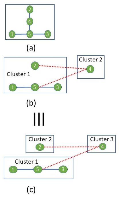
Figure 1: An example to illustrate equivalence of disconnected clusters to higher-order connected clusters: (a) the thermal network, (b) disconnected two-cluster partition, (c) equivalent (in terms of decentralized control) connected three-cluster partition.

Next, we preset the size and relative size constraints in (4) regarding the obtained clusters. Such constraints are important for the management of the computational load of cluster level control design and/or its sensitivity to any fault.

$$\displaystyle\underline{M}_{a}\leq\displaystyle\sum_{i\in V}p_{i,c}\leq\bar{M}_{a},\,c\in\mathcal{C},$$ (4a)

$$\displaystyle\left|\sum_{i\in V}p_{i,c_{a}}-\sum_{i\in V}p_{i,c_{b}}\right|\leq M_{r},\,c_{a},c_{b}\in\mathcal{C},\,a\neq b.\,$$ (4b)

Finally, we express the expression for the objective function and its minimization in (5). Here, we try to minimize the sum of edge weights (which are thermal interaction levels lying inside intervals) for edges not belonging to any cluster. The decision variables $p,s,r$ are the vectors with entries from $p_{i,c},s_{i,j,c},r_{i,j}$, respectively.

$$J=\min_{r}\sum_{\begin{subarray}{c}(i,j)\in E,\\ \mu_{i,j}\in I_{i,j}\end{subarray}}(1-r_{i,j})\mu_{i,j}$$ (5)

Letting $p\triangleq[\{p_{i,c}\}]\in\{0,1\}^{N_{z}\times n}$, $s\triangleq[\{s_{i,j,c}\}]\in\mathbb{R}_{+}^{|E|\times n}$, $r\triangleq[\{r_{i,j}\}]\in\mathbb{R}_{+}^{|E|}$, and $\mu\triangleq[\{\mu_{i,j}\}]\in\mathbb{R}_{+}^{|E|}$, we can write the optimization problem consisting of the objective function minimization given by (5) and constraints given (3a)- (3j) & (4a)-(4b) as in (II-C).

$$\min_{r}\,(1-r)^{T}\mu,\quad\mu\in I\subseteq\mathbb{R}_{+}^{|E|}$$

subject to

$$\underbrace{\left(\begin{array}[]{ccc}A_{p}^{1}&0&0\\ 0&A_{s}^{1}&0\\ A_{p}^{2}&A_{s}^{2}&0\\ 0&A_{s}^{3}&A_{r}^{1}\\ 0&0&A_{r}^{2}\\ \end{array}\right)}_{A\in\mathbb{Z}^{d_{1}\times d_{2}}}\left(\begin{array}[]{c}p\\ r\\ s\\ \end{array}\right)\leq b,$$ (14)

$$p\in\{0,1\}^{N_{z}\times n},\,s\in\mathbb{R}_{+}^{|E|\times n},\,r\in\mathbb{R}_{+}^{|E|},$$

where $I$ is the thermal interaction interval vector, the dimensions of $A$ are $d_{1}=2(N_{z}+n^{2})+|E|(3n+5),\,d_{2}=N_{z}n+|E|(n+1)$, and in $A$ the first block row corresponds to (3a) & (4), the second block row to (3b), the third block row to (3c)-(3e), the fourth block row to (3f), and the fifth block row to (3g).

In the next sections, we will present a stochastic optimization approach and a robust optimization approach to formulate the uncertainty in the objective function.

II-D A stochastic optimization approach to optimal clustering

In the stochastic optimization framework, the goal is to minimize the expectation of the cost since the constraints are deterministic and the cost function is the only part involving uncertainty. As a result, in (5) we replace all the cost coefficients by their expectation. To that end, let each interval $I_{ij}$ be divided into $n_{d}$ sub-intervals and let $\hat{I}_{ij,k}$ represent the mean of $k$-th sub-interval with its probability of occurrence $P_{ij,k}$, $k\in\{1,2,\cdots,n_{d}\}$. Defining $\displaystyle\mu_{ij}^{s}\triangleq\bigg{[}\Big{\{}\sum_{k=1}^{n_{d}}P_{ij,k}\hat{I}_{ij,k}\Big{\}}\bigg{]}$, $\mu^{s}\triangleq[\{\mu_{i,j}\}]\in\mathbb{R}_{+}^{|E|}$, the stochastic formulation of the optimization problem becomes

$$\min_{r}\,(1-r)^{T}\mu^{s}$$

subject to

$$A\left(\begin{array}[]{c}p\\ r\\ s\\ \end{array}\right)\leq b,$$ (18)

$$p\in\{0,1\}^{N_{z}\times n},\,s\in\mathbb{R}_{+}^{|E|\times n},\,r\in\mathbb{R}_{+}^{|E|}.$$

II-E A robust optimization approach to optimal clustering

In this section, we will present the robust optimization version of the mixed 0,1 LP problem in (II-C), which has an uncertain objective function due to the uncertainty in $\mu$. As a first step, by letting $(1-r)^{T}\mu\leq z$ and minimizing $z$ (the new objective function and new variable), we transform the original objective function into a constraint. Next, defining $\bar{\mu}\triangleq(\mu_{max}+\mu_{min})/2$ and $\mu_{mg}\triangleq\mu_{max}-\bar{\mu}$, we can write the interval uncertainty vector as $I=\bar{\mu}+\text{diag}(\varepsilon_{1},\cdots,\varepsilon_{|E|})\mu_{mg}$, where the entries of the random diagonal matrix satisfy $\big{|}\varepsilon_{i}\big{|}\leq 1$. Following the lines in [22, 23] for transformation of a robust MILP into an equivalent deterministic MILP (called the “robust counterpart"), we obtain the robust counterpart as in (II-E):

$$\hskip 68.28644pt\min_{z}\ z$$

subject to

$$\underbrace{\left(\begin{array}[]{r:ccc}-1&0&-(\bar{\mu}+\mu_{mg})^{T}&0\\ \hdashline 0&A_{p}^{1}&0&0\\ 0&0&A_{s}^{1}&0\\ 0&A_{p}^{2}&A_{s}^{2}&0\\ 0&0&A_{s}^{3}&A_{r}^{1}\\ 0&0&0&A_{r}^{2}\\ \end{array}\right)}_{\tilde{A}\in\mathbb{Z}^{(d_{1}+1)\times(d_{2}+1)}}\left(\begin{array}[]{c}z\\ \hdashline p\\ r\\ s\\ \end{array}\right)$$ (29)

$$\hskip 142.26378pt\leq\underbrace{\left(\begin{array}[]{c}(\mu_{mg}-\bar{\mu})^{T}1\\ \hdashline b\\ \end{array}\right)}_{\tilde{b}},$$ (32)

$$z\in\mathbb{R}_{+},\,p\in\{0,1\}^{N_{z}\times n},\,s\in\mathbb{R}_{+}^{|E|\times n},\,r\in\mathbb{R}_{+}^{|E|}.$$

II-F Definition of performance index and optimality deterrioration/fault propagation metrics

The performance of any control architecture will be measured through the following performance index (PI):

$$\text{PI}\triangleq e^{-k_{u}\frac{u_{tot}}{u_{tot-nr}}}\times e^{-k_{y_{v-ave}}\frac{y_{v-ave}}{y_{v-ave-nr}}}\times e^{-k_{y_{v-max}}\frac{y_{v-max}}{y_{v-max-nr}}},$$ (33)

where the first term takes into account the effect of total consumed energy, the second term the effect of average comfort temperature violation over all zones and the period over which the system is controlled, and the final term the effect of maximum comfort temperature violation; $k_{u},k_{y_{v-ave}},k_{y_{v-max}}$ are weight parameters; $u_{tot-nr},y_{v-ave-nr},y_{v-max-nr}$ are parameters used for normalization. Note that PI=1 when $u_{tot}=0$ and no comfort temperature violation, which is impossible in practice. As a result, PI=1 is an ideal bound, but the closer PI is to 1, the better the performance of that control architecture is. The only constraint on the weights $k_{u},k_{y_{v-ave}},k_{y_{v-max}}$ is that PI($1$, no-fault) ($n=1$ corresponds to C-MPC) should have the largest value compared to all other MPC architectures with/without faults, since fault-free C-MPC is the best solution.

Next, we define two metrics that measure the optimality and sensitivity to fault propagation of a given control architecture corresponding to a “best n-partition ($\text{n}^{\star}$)". The first metric is called the “optimality deterioration metric" (ODM) defined as

$$\text{ODM}(\text{n}^{\star},\text{no-fault})\triangleq\frac{\text{PI(1, no-fault)}-\text{PI}(\text{n}^{\star},\text{no-fault})}{\text{PI(1, no-fault)}},$$ (34)

where $\text{PI}(\text{n}^{\star},\text{no-fault})$ denotes the performance index of the control architecture corresponding to the best $n$-partition under no fault. The second metric called “fault propagation metric" (FPM) will be used to quantitatively determine the sensitivity of an MPC architecture to a fault in control/measurement equipment in a zone. This metric is defined as

$$\text{FPM}(\text{n}^{\star},\text{fault})\triangleq\frac{\text{PI(1, no-fault)}-\text{PI}(\text{n}^{\star},\text{fault})}{\text{PI(1, no-fault)}}.$$ (35)

Finally, we need to determine which best n-partition is the best partition. To that end, we define a weighted-performance metric (WPM) as

$$\text{WPM}(\text{n}^{\star})\triangleq \alpha(1-\text{ODM}(\text{n}^{\star},\text{no-fault}))+$$

$$(1-\alpha)(1-\text{FPM}(\text{n}^{\star},\text{fault})),$$ (36)

where $0\leq\alpha\leq 1$ is a user-parameter. Then, the best n-partition is the one which has the highest WPM value.

Remark (Expected performance).

The paradigm of the presented approach is based on the realistic intuition that the lower the level of thermal interaction between clusters, the more likely higher WPM values for the decentalizedly controlled clusters. However, there is no guarantee for this.

III Case studies

In this section we will consider two case studies to demonstrate the developed optimal partitioning approach. Due to space limitations, we will present the results only for the stochastic optimization version. The first case study is a small-scale multi-zone building, which allows one to analyse all possible connected partitions for post-assessment (testing the decentralized controller corresponding to the associated partitioning) and to determine the success rate of the partitioning method. In both case studies, it was assumed that comfort range is [22, 24] °C and that each zone temperature can be controlled with a separate heater/cooler. In D-MPC designs, we had the following assumptions: for a given cluster, interaction temperatures between zones in that cluster and neighbor zones in other clusters were set to 23 °C (the middle value in the comfort range); the prediction horizon was taken as 6 hours; the only constraint was to keep zone temperatures in the comfort band whenever possible; the cost function was the weighted sum of total energy consumption and comfort temperature violation where the weight used for comfort temperature violation penalization was $10^{6}$ times the weight used for each control input ($w_{u_{i}}=1$). In applying the developed partitioning approach to the case studies, we did not use any size and relative size constraints on the formed clusters.

III-A Case study 1

This case study, shown in Figure 2, is a 5-zone office building used during 8:00-18:00. There are significant openings between Z1-Z5, Z3-Z5, and Z4-Z5 which are modeled by pure resistors. The resistance between Z4-Z5 is taken as $R=0.1m^{2}K/W$ and the resistances between Z1-Z5 and Z3-Z5 are scaled multiples of $R$ where scales are ratios of volumes of Z1 and Z5 to volume of Z4. The thermal interaction intervals for this case study are: $\text{I}_{\text{1-5}}=[0.0134,2.026]$°C, $\text{I}_{\text{2-4}}=[0.0013,0.136]$°C, $\text{I}_{\text{3-5}}=[0.0148,2.36]$°C, $\text{I}_{\text{4-5}}=[0.0171,1.79]$°C. The thermal interaction distributions together with their mean values are given in Figure 3, which shows that there is no specific pattern. Optimal n-partitions determined from the developed approach are presented in Figure 4.

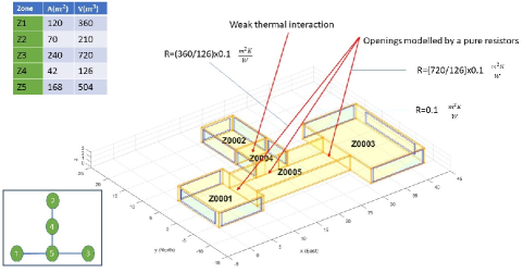
Figure 2: A five-zone building, its data and thermal interaction network.

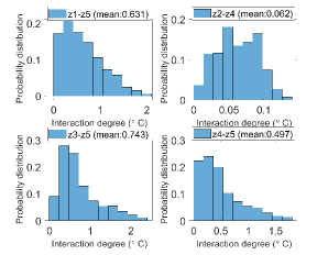
Figure 3: Thermal interaction distributions over one year for the first case study.

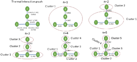
Figure 4: Optimal n-partitions for the first case study. Interval and single numbers on edges represent thermal interaction intervals and their mean, respectively.

To determine whether the optimal n-partitions are really optimal we designed D-MPCs for all possible connected clusters including the optimal n-partitions. For this case study we considered three scenarios: S1-all zone temperatures are controlled, S2-Z1-Z4 controlled, Z5 uncontrolled (to investigate the thermal effect of an uncontrolled zone on controlled zones), and S3-there is $\pm$ 10% error in zone air temperature sensor for all zones but one zone at a time (to investigate the effect of fault propagation). The 5-zone building was controlled to keep the zone temperatures in the comfort band. We calculated the average energy per day and per zone ($u_{tot}$), average temperature violation ($y_{v-ave}$) and maximum temperature violation ($y_{v-max}$). The results for S1, S2 and S3 for all possible connected partitions are given in the specified columns in Table I which also includes the ODM, FPM and WPM when all zones are controlled. The weight parameters were taken as $k_{u}=k_{y_{v-ave}}=k_{y_{v-max}}=1$; $u_{tot-nr}=100\text{ kWh},y_{v-ave-nr}=1\textdegree{C},y_{v-max-nr}=3\textdegree{C}$; $\alpha=0.5$.

TABLE I: Post-evaluation results (over one day) for all connected partitions. The comfort range for controlled zones is [22, 24]°C during 8:00-18:00.

n and partition		Z1-Z5 controlled			Z1-Z4 controlled			Faulty case			Metrics
n	partition	$\text{u}_{\text{tot}}$ (kWh)	$\text{y}_{\text{v-ave}}$ (°C)	$\text{y}_{\text{v-max}}$ (°C)	$\text{u}_{\text{tot}}$ (kWh)	$\text{y}_{\text{v-ave}}$ (°C)	$\text{y}_{\text{v-max}}$ (°C)	$\text{u}_{\text{tot}}$ (kWh)	$\text{y}_{\text{v-ave}}$ (°C)	$\text{y}_{\text{v-max}}$ (°C)	ODM (%)	FPM (%)	WPM (%)
1	{1,2,3,4,5}	58.9649	0	0	49.0952	0	0	58.7341	0.1608	2.0582	0	57.026	71.487
2	{1,2,4,5},{3}	58.1501	0.0084	0.0525	48.2976	0.0072	0.1215	58.7303	0.1594	1.9429	1.762	55.277	71.481
2	{1,3,4,5},{2}	58.9643	0.0001	0.0004	49.0945	0.0001	0.0004	58.6829	0.1581	1.8642	0.016	54.007	72.989
2	{1,3,5},{2,4}	58.8276	0.0036	0.0382	48.9677	0.0055	0.1101	58.6496	0.1587	1.9275	1.488	54.978	71.767
2	{1},{2,3,4,5}	57.0280	0.0276	0.1934	47.1860	0.0293	0.5173	58.6615	0.1645	1.8398	7.012	53.917	69.536
3	{1,3,5},{2},{4}	58.8270	0.0037	0.0386	48.9672	0.0055	0.1105	58.6340	0.1602	1.8411	1.504	53.726	72.385
3	{1,4,5},{2},{3}	58.1495	0.0084	0.0525	48.2969	0.0072	0.1215	58.6336	0.1606	1.8893	1.764	54.483	71.876
3	{1,5},{2,4},{3}	58.0123	0.0121	0.0630	48.1740	0.0126	0.1215	58.6649	0.1607	1.8526	2.325	53.942	71.866
3	{1},{2,4,5},{3}	56.2089	0.0361	0.1987	46.4418	0.0359	0.5176	58.6844	0.1666	1.8074	7.203	53.526	69.636
3	{1},{2,4},{3,5}	56.8894	0.0313	0.1945	47.0676	0.0346	0.5173	58.5631	0.1672	1.8889	7.258	54.741	69.000
3	{1},{2},{3,4,5}	57.0274	0.0276	0.1934	47.1854	0.0293	0.5173	58.5562	0.1678	1.7497	7.014	52.619	70.184
4	{1},{2,4},{3},{5}	56.0699	0.0398	0.1998	46.3273	0.0410	0.5176	58.5528	0.1708	1.8716	7.449	54.639	68.956
4	{1,5},{2},{3},{4}	58.0118	0.0121	0.0630	48.1734	0.0126	0.1215	58.8271	0.1597	1.7811	2.327	52.860	72.406
4	{1},{2},{3,5},{4}	56.8888	0.0313	0.1945	47.0670	0.0346	0.5173	58.6167	0.1687	1.8067	7.260	53.579	69.581
4	{1},{2},{3},{4,5}	56.2083	0.0361	0.1987	46.4412	0.0359	0.5176	58.7196	0.1674	1.7254	7.205	52.292	70.252
5	{1},{2},{3},{4},{5}	56.0693	0.0398	0.1998	46.3267	0.0410	0.5176	58.3571	0.1711	1.8167	7.450	53.723	69.413

III-B Case study 2

The second case study is a 20-zone building with a large number of thermally interacting zones. The building and its thermal interaction graph are shown in Figure 5. For this case study we considered two scenarios: S1-all zone temperatures are controlled, and S2-to investigate the effect of fault propagation, we now assumed a different type of a likely fault: we assumed that actuators at each zone fail, one at a time, so that no heat/cold is supplied ($u_{i}$=0). The results are given in Table II. The weight parameters were taken as $k_{u}=k_{y_{v-ave}}=k_{y_{v-max}}=1$; $u_{tot-nr}=1000\text{ kWh},y_{v-ave-nr}=2\textdegree{C},y_{v-max-nr}=5\textdegree{C}$; $\alpha=0.5$.

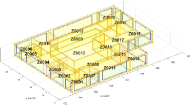
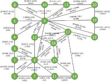
Figure 5: (a) A twenty-zone building and (b) its thermal interaction network. The values in parenthesis are mean values. Note that zone 9 has 11 thermal interactions.

TABLE II: Post-evaluation results (over one day) for all best partitions. The comfort range for all zones is [22, 24]°C during 8:00-18:00.

	Z1-Z20 controlled			Faulty case			Metrics
$\text{n}^{\star}$	$\text{u}_{\text{total}}$(kWh)	$\text{y}_{\text{v-ave}}$ (°C)	$\text{y}_{\text{v-max}}$(°C)	$\text{u}_{\text{total}}$(kWh)	$\text{y}_{\text{v-ave}}$(°C)	$\text{y}_{\text{v-max}}$(°C)	ODM (%)	FPM (%)	WPM (%)
$\text{1}^{\star}$	795.5808	0	0	823.3647	0.1104	3.1123	0	50.6112	74.6944
$\text{2}^{\star}$	795.5657	0.0001	0.0006	823.3480	0.1105	3.1125	0.0127	50.6133	74.6870
$\text{3}^{\star}$	795.5608	0.0001	0.0007	823.3427	0.1105	3.1125	0.0143	50.6136	74.6861
$\text{4}^{\star}$	795.5601	0.0001	0.0007	823.3417	0.1105	3.1125	0.0155	50.6139	74.6853
$\text{5}^{\star}$	795.5499	0.0001	0.0017	823.3302	0.1105	3.1128	0.0346	50.6168	74.6743
$\text{6}^{\star}$	795.5481	0.0001	0.0017	823.3282	0.1105	3.1128	0.0345	50.6167	74.6744
$\text{7}^{\star}$	795.5144	0.0002	0.0017	823.2911	0.1106	3.1128	0.0342	50.6172	74.6743
$\text{8}^{\star}$	795.5106	0.0002	0.0018	823.2866	0.1106	3.1129	0.0378	50.6178	74.6722
$\text{9}^{\star}$	795.5081	0.0002	0.0018	823.2839	0.1106	3.1129	0.0379	50.6178	74.6721
$\text{10}^{\star}$	795.5057	0.0002	0.0018	823.2815	0.1106	3.1129	0.0380	50.6179	74.6721
$\text{11}^{\star}$	795.4738	0.0003	0.0030	823.2476	0.1107	3.1132	0.0621	50.6218	74.6581
$\text{12}^{\star}$	730.4916	0.2251	2.0331	756.3917	0.3330	3.7592	36.4961	58.4863	52.5088
$\text{13}^{\star}$	709.5264	0.2912	2.3103	733.9544	0.3987	3.8677	40.6440	59.7976	49.7792
$\text{14}^{\star}$	686.2700	0.3751	3.2300	710.2009	0.4793	4.2173	51.5292	63.1284	42.6712
$\text{15}^{\star}$	683.6270	0.3855	3.3964	707.2868	0.4904	4.2870	53.2361	63.7347	41.5146
$\text{16}^{\star}$	641.7458	0.4901	3.3964	663.0952	0.5903	4.2768	53.7213	63.8693	41.2047
$\text{17}^{\star}$	610.2526	0.6849	3.3965	630.5260	0.7778	4.2813	56.6738	66.0434	38.6414
$\text{19}^{\star}$	601.1079	0.7466	3.3965	621.0750	0.8379	4.3016	57.6042	66.8703	37.7627
$\text{19}^{\star}$	571.9436	0.8562	3.3966	590.7952	0.9422	4.3017	58.6784	67.5875	36.8670
$\text{20}^{\star}$	550.9360	1.0015	4.3932	569.1118	1.0813	4.7148	67.8492	71.5529	30.2989

III-C Discussions of results

The computation time for each partitioning in both case studies is less than one minute using a laptop with the following hardware specifications: 8GB RAM, Intel(R) Core(TM) i7-8550U CPU @ 1.80GHz 1.99 GHz. CPLEX was used as the solver in the solution of the mixed-integer linear programs. From Table I of Case Study 1 we observe that, when all zone temperatures are controlled, all control architectures (C-MPC and D-MPC) have performances which are close to each other on the basis of WPM, even though the building in case study 1 is a highly thermally-interacting structure to due large openings between zones. The explanation for such an observation is the fact that when all zone temperatures are controlled in a narrow band, then the thermal interaction is not significant, even though the building has a huge potential for thermal interaction. When one of the zones was not controlled in Case Study 1, we observe from Table I that temperature violation increases in D-MPC cases since thermal interactions increase, but the performance of D-MPCs (based on WPM) are still acceptable. In Table I green rows indicate the best partition of each n-partition. When these results are compared with the optimal partitioning results in Figure 4, which are results predicted by our approach, we see that out of five best n-partitions, four of them are predicted correctly. However, since there is only one possible partition when $n=1,5$, it will be more correct to say that out of three best partitions, two of them are predicted correctly by our developed approach with a success rate of 66.7%. Based on the WPM, the best control architecture for the first case study is $n^{\star}=2$ with the zone partition $\{2\},\{1,3,4,5\}$.

As regards to the second case study, we see from Table II that the best control architecture predicted by our OLBP approach based on WPM is C-MPC. However, note that the performance of D-MPC with $n^{\star}=11$ is very close to that of C-MPC, which again shows that a D-MPC control architecture can work quite well in control of multi-zone buildings.

IV Conclusions

In this paper, we presented an approach for optimal partitioning of multi-thermal zone buildings for decentralized control. Both stochastic and robust optimization versions of the developed approach were presented, and the stochastic version of the algorithm was demonstrated on two case studies. The first case study was a small-scale example so that we were able to obtain all possible partitions and post-asses the performance of the corresponding controllers. From the post-assessment, we observed that the success rate of our optimal partitioning algorithm is $66.7\%$, quite good when the difficulty and complexity of the optimal partitioning problem are considered. Next, we tested the method on a 20-zone building and determined the optimal partitioning predicted for this building. Moreover, in this paper we presented new metrics (optimality deterioration and fault propagation metrics) which can be used in a general decentralized control framework.

The most important findings of this study can be listed as follows: (i) the presented partitioning algorithm can be used effectively to determine the best partition and the corresponding decentralized control architecture for multi-zone buildings; (ii) decentralized control can work very well in office buildings (even for cases where there is a high potential for thermal interaction between zones) since zone temperatures are, in general, strictly controlled in these buildings during working hours, and as a result, thermal interactions are not significant (except in the morning during the short period when controllers start to move the uncontrolled zone temperatures to the comfort band); (iii) since decentralized control can work quite well for office buildings, for this category of buildings one can use a decentralized control-oriented modeling approach per zone cluster, which will ease the current bottle-neck (the considerable effort in control model development [24]) for the wide-spread application of MPC in office buildings; (iv) for multi-zone buildings, it is not always correct that D-MPC will outperform C-MPC in case of fault propagation: the faults stay more local in D-MPC compared to C-MPC but since the control models in D-MPC are less accurate (since they are not able to take all thermal interactions into account) the real performance of D-MPC depends on a combination of these two effects in faulty scenarios.

A future research direction is to consider a co-design approach where MPC design is explicitly integrated into the partitioning problem. This approach, although computationally expensive, has a huge potential to outperform the approach presented here.

References

- [1] F. Oldewurtel, A. Parisio, C. N. Jones, D. Gyalistras, M. Gwerder, V. Stauch, B. Lehmann, and M. Morari, “Use of model predictive control and weather forecasts for energy efficient building climate control", Energy and Buildings, vol. 45, pp. 15-27, February 2012.
- [2] F. Oldewurtel, C. N. Jones, A. Parisio, and M. Morari, “Stochastic model predictive control for building climate control", IEEE Transactions on Control Systems Technology, vol. 22, no. 3, pp. 1198-1205, 2014.
- [3] E. Atam, “New Paths Toward Energy-Efficient Buildings: A Multiaspect Discussion of Advanced Model-Based Control", IEEE Industrial Electronics Magazine, vol. 10, no. 4, pp. 50-66, 2016.
- [4] E. Atam, “Investigation of computational speed of Laguerre network-based MPC in thermal control of energy-efficient buildings", Turkish Journal of Electrical Engineering & Computer Sciences, vol. 25, pp. 4369-4380, 2017.
- [5] S. Privara, J. Siroky, L. Ferkl, and J. Cigler, “Model predictive control of a building heating system: the first experience", Energy and Buildings, vol. 43, no. 2, pp. 564-572, 2011.
- [6] D. Sturzenegger, D. Gyalistras, M. Gwerder, C. Sagerschnig, M. Morari, and R. Smith, “Model Predictive Control of a Swiss Office Building", Clima - RHEVA World Congress, June 15-19, Prague, Czech Republic, pp. 3227-3236, 2013.
- [7] B. Dong and K. H. Lam, “A real-time model predictive control for building heating and cooling systems based on the occupancy behavior pattern detection and local weather forecasting", Building Simulation, vol. 7, pp. 89-106, 2014.
- [8] S. C. Bengea, A. D. Kelman, F. Borrelli, R. Taylor, and S. Narayanan, “Implementation of model predictive control for an HVAC system in a mid-size commercial building", HVAC& R Research, vol. 20, no. 1, pp. 121-135, 2014.
- [9] E. Atam, “Decentralized thermal modeling of multi-zone buildings for control applications and investigation of submodeling error propagation", Energy and Buildings, vol. 16, pp. 384-395, 2016.
- [10] J. Cai and J. E. Braun, “A practical and scalable inverse modeling approach for multi-zone buildings", 9th International Conference on System Simulation in Buildings, Liege, Belgium, December 10-12, 2014.
- [11] C. Agbi, “Scalable and robust designs of model-based control strategies for energy-efficient buildings", PhD Thesis, Carnegie Mellon University, 2014, Available online: http://www.researchgate.net/publication/285581350_Scalable_and_Robust_Design_of_Model-Based_Control_Strategies_for_Energy_Efficient_Buildings.
- [12] J. F. M. Van Doren, S. G. Douma, P. M. J. Van den Hof, J. D. Jansen, and O. H. Bosgra, “Identifiability: from qualitative analysis to model structure approximation," in Proceedings of the 15th International Federation on Automatic Control (IFAC) Symposium on System Identification, Saint-Malo, France, July 6-8 2009, pp. 664-669.
- [13] J. F. M. Van Doren, P. M. J. Van den Hof, J. D. Jansen, and O. H. Bosgra, “Parameter identification in large-scale models for oil and gas production," in Proceedings of 18th In- ternational Federation on Automatic Control (IFAC) World Congress, Milano, Italy, August 28-September 2 2011, pp. 10857-10862.
- [14] A. Kyriacou, S. Timotheeou, M. P. Michaelides, C. Panayiotou, and M. Polycarpou, “Partitioning of intelligent buildings for distributed contamination detection and isolation," IEEE Transcations on Emerging Topics in Compuational Intelligence, vol. 1, no. 2, pp. 72-86, 2017.
- [15] V. Chandan and A. Alleyne, “Optimal partitioning for the decentralized thermal control of builings," IEEE Transcations on Control Systems Technology, vol. 21, no. 5, pp. 1756-1170, 2013.
- [16] D. Sturzenegger, D. Gyalistras, V. Semeraro, M. Morari and R. S. Smith, “BRCM Matlab toolbox: model generation for model predictive building control", American Control Conference, June 4-6, Portland, USA, pp. 1063-1069, 2014.
- [17] D. B. Crawley, L. K Lawrie, C. O Pedersen and F. C. Winkelmann. “EnergyPlus: energy simulation program", ASHRAE Journal, vol. 42, pp. 49-56, 2000.
- [18] M. Boulle, “Compact mathematical formulation for graph partitioning," Optiiozation and Engineering, vol.5, pp. 315-333, 2014.
- [19] T.Shirabe, “A model of contiguity for spatial unit allocation," Geographical Analysis, vol. 37, pp. 2-16, 2005.
- [20] J. Conrad, C. P. Gomes, W. J. van Hoeve, A. Sabharwal and J. Suter, “Connections in networks: hardness of feasibility versus optimality," In Integration of AI and OR Techniques in Constraint Programming for Combinatorial Optimization Problems, Springer, pp. 16-28, 2007.
- [21] B. Dilkina and C. P. Gomes, “Solving connected subgraph problems in wildlife conservation," In: A. Lodi, M. Milano, P. Toth (eds.) CPAIOR, LNCS, vol. 6140, pp. 102-116, 2010.
- [22] D. Bertsimas and M. Sim, “The price of robustness," Operations Research, vol. 52, no. 1, pp. 35-53, 2004.
- [23] Z. Li, R. Ding, C. A. Floudas, “A comparative theoretical and computational study on robust counterpart optimization: I. Robust linear optimization and robust mixed integer linear optimization,", Ind Eng Chem Res, vol.50, pp. 10567-10603, 2011.
- [24] E. Atam and L. Helsen “Control-oriented thermal modeling of multi-zone buildings: Methods and issues", IEEE Control Systems Magazine, vol. 36, no. 3, pp. 86-111, 2016.