Hypernetwork-Based Augmentation

Abstract

Data augmentation is an effective technique to improve the generalization of deep neural networks. Recently, AutoAugment [5] proposed a well-designed search space and a search algorithm that automatically finds augmentation policies in a data-driven manner. However, AutoAugment is computationally intensive. In this paper, we propose an efficient gradient-based search algorithm, called Hypernetwork-Based Augmentation (HBA), which simultaneously learns model parameters and augmentation hyperparameters in a single training. Our HBA uses a hypernetwork to approximate a population-based training algorithm, which enables us to tune augmentation hyperparameters by gradient descent. Besides, we introduce a weight sharing strategy that simplifies our hypernetwork architecture and speeds up our search algorithm. We conduct experiments on CIFAR-10, CIFAR-100, SVHN, and ImageNet. Our results show that HBA is competitive to the state-of-the-art methods in terms of both search speed and accuracy.

1 Introduction

Data augmentation techniques, such as cropping, horizontal flipping, and color jittering, are widely used in training deep neural networks for image classification. Data augmentation acts as a regularizer that reduces overfitting by transforming images to increase the quantity and diversity of training data. Recently, data augmentation has shown to be an effective technique not only for supervised learning [5, 12, 20], but also for semi-supervised learning [29, 2], self-supervised learning [4], and reinforcement learning (RL) [16]. However, given a new task or dataset, it is non-trivial to either manually or automatically design its data augmentation policy: determine a set of augmentation functions and adequately specify their configurations, such as the range of rotation, the size of cropping, the degree of color jittering. A weak augmentation policy may not help much, while a strong one could hinder performance by making an augmented image looks inconsistent to its label.

AutoAugment [5], a representative pioneering work proposed by Cubuk et al., proposed a search space (consisting of 16 image operations) and an RL-based search algorithm to automate the process of finding an effective augmentation policy over the search space. AutoAugment made remarkable improvements in image classification. However, its search algorithm requires $5000$ GPU hours for one augmentation policy learning, which is extremely computationally intensive.

Dataset		AA	PBA	FAA	HBA
CIFAR-10	GPU Hours	$5000$	$5$	$3.5$	$0.1$
	Test Error $(\%)$	$2.6$	$2.6$	$2.7$	$2.6$
SVHN	GPU Hours	$1000$	$1$	$1.5$	$0.1$
	Test Error $(\%)$	$1.1$	$1.2$	$1.1$	$1.1$
ImageNet	GPU Hours	$15000$	-	$450$	$0.9$
	Test Error $(\%)$	$22.4$	-	$22.4$	$22.1$

Table 1: Hypernetwork-Based Augmentation (HBA) is at least an order of magnitude faster than AutoAugment (AA) [5], Population Based Augmentation (PBA) [12], and Fast AutoAugment (FAA) [20], while achieving similar accuracy.

To address the computational issue, we formulate the augmentation policy search problem as a hyperparameter optimization problem and propose an efficient algorithm for tuning data augmentation hyperparameters. The central idea of our method is a novel combination of a population-based training algorithm and a hypernetwork, which is a function that outputs the weights of a neural network. In particular, we introduce a population-based training procedure and four modifications to derive our algorithm. First, we employ a hypernetwork to represent the set of models. By doing so, training a hypernetwork can be treated as training a continuous population of models. Second, we propose a new hyper-layer for batch normalization [13] to facilitate the construction of hypernetworks. Third, inspired by one-shot neural architecture search [26, 3, 1], we adopt a weight sharing strategy to the models. We show that such a strategy corresponds to a simplified hypernetwork architecture that effectively reduces the search time. Fourth, instead of evaluating the performance on the discrete set of models, thanks to the use of a hypernetwork, we perform gradient descent to efficiently find the approximate best model. Our method, dubbed as Hypernetwork-Based Augmentation (HBA), is a gradient-based method that jointly trains the network model and tunes the augmentation hyperparameters. HBA yields hyperparameter schedules that can be used to train on different datasets or to train different network architectures. Experimental results show that HBA achieves significantly faster search speed while maintaining competitive accuracy. Table 1 summarizes our main results.

Our contributions can be summarized as follows. (1) We propose Hypernetwork-Based Augmentation (HBA), an efficient gradient-based method for automated data augmentation. (2) The derivation of HBA reveals the underlying relationship between population-based and gradient-based methods. (3) We propose a weight-sharing strategy that simplifies our hypernetwork architecture and reduces the search time considerably without performance drop.

2 Related work

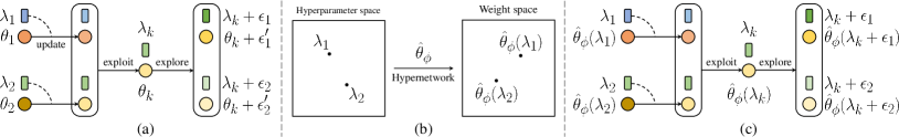
Figure 1: (a) A population-based training (PBT) trains a discrete set of models and performs exploitation followed by exploration to tune data augmentation hyperparameters. In this example, two models are updated, and the second one is exploited and explored. Section 3.1 explains the details. (b) We employ a hypernetwork $\hat{\theta}_{\phi}$ to represent the set of models $\{\theta_{1},\theta_{2}\}$ by $\{\hat{\theta}_{\phi}(\lambda_{1}),\hat{\theta}_{\phi}(\lambda_{2})\}$, where $\hat{\theta}_{\phi}$ is a continuous function that aims to map from each model $i$’s hyperparameters $\lambda_{i}$ to its weights $\theta_{i}$. (c) We show the resulting schematic diagram of training a single hypernetwork that approximates a population-based training. Section 3.2 details the modified training algorithm, and Section 3.3 describes the hypernetwork architecture.

Data Augmentation. We review previous work relevant to the development of our method. We refer readers to a comprehensive survey paper [27] on data augmentation. Hand-designed data augmentation techniques, such as horizontal flipping, random cropping, and color transformations, are commonly used in training deep neural networks for image classification [18, 11]. In recent years, several effective data augmentation techniques are proposed. Cutout [8] randomly erases contents by sampling a patch from the input image and replace it with a constant value. Mixup [34] performs data interpolation that combines pairs of images and their labels in a convex manner to generate virtual training data. CutMix [32] generates new samples by cutting and pasting image patches within mini-batches. These data augmentation techniques are hand-designed, and their hyperparameters are usually manually-tuned.

Automated Data Augmentation. Inspired by recent advances in neural architecture search [36, 26, 22], one of the recent trends in data augmentation is automatically finding augmentation policies within a pre-defined search space in a data-driven manner. AutoAugment [5] introduced a well-designed search space and proposed an RL-based search algorithm that trains a recurrent neural network (RNN) controller to search effective augmentation policies within the search space. Although AutoAugment achieves promising results, its search process is computationally expensive (5000 GPU hours on CIFAR-10). Our algorithm treats the data augmentation hyperparameters as continuous variables, and efficiently optimizes them by gradient descent in a single round of training.

Recently, several efficient search algorithms based on AutoAugment’s search space have been proposed. Population Based Augmentation (PBA) [12] employed Population Based Training (PBT) [14], an evolution-based hyperparameter optimization algorithm, to search data augmentation schedules. Fast AutoAugment [20] treats the problem as a density matching problem and used Bayesian optimization to find augmentation policies. OHL-Auto-Aug [21] proposed an online hyperparameter learning algorithm that jointly learns network parameters and augmentation policy. Our algorithm also tunes augmentation hyperparameters in an online manner while achieving better search efficiency. RandAugment [6] simplified the search space of AutoAugment and used the grid search method to find the optimal augmentation policy. Differentiable Automatic Data Augmentation (DADA) [19], inspired by Differentiable Architecture Search (DARTS) [22], proposed a gradient-based method that relaxes the discrete policy selection to be differentiable and optimize the augmentation policy by stochastic gradient descent. Our algorithm is also gradient-based but is fundamentally different from DADA. DADA realizes relaxation by the Gumbel-softmax trick, while ours is based on combining population-based training and hypernetworks.

Hypernetworks. Ha et al. [10] used hypernetworks to generate weights for recurrent networks. SMASH [3] presented a gradient-based neural architecture search method that employs a hypernetwork to learn a mapping from a binary-encoded architecture space to the weight space. Self-Tuning Network (STN) [23] used a hypernetwork as an approximation to the best response function in bilevel optimization. Our method uses a hypernetwork to represent a set of models trained with different hyperparameters.

Hyperparameter Optimization. Searching augmentation policies can be formulated as a hyperparameter optimization problem. We refer readers to a recent survey paper [31] on hyperparameter optimization. Population Based Training (PBT) [12] presented a hyperparameter optimization algorithm that trains a population of models in parallel, and periodically evaluates their performance to perform exploitation and exploration. MacKay et al. proposed the Self-Tuning Network (STN) [23], a gradient-based method for tuning regularization hyperparameters, including data augmentation and dropout [28].

HBA is closely related to PBT [14] and STN [23]. In our method, we start from a population-based training algorithm and apply a series of modifications to derive our algorithm, which can be viewed as an efficient approximation of the PBT algorithm. Compared with STN, HBA distinguishes from STN in three aspects. First, the underlying formulations are different. STN is based on the best response approximation to bilevel optimization, while HBA is derived entirely from the perspective of population-based training. Second, HBA adopts a weight sharing strategy, which is intuitive yet novel since it cannot be analogously defined in STN. Third, to facilitate the construction of hypernetworks, we propose a new hyper-layer for batch normalization.

3 Method

We start from a population-based training (Section 3.1) and then present a series of modifications to derive HBA: hypernetworks (Section 3.2 and 3.3), weight sharing strategy (Section 3.4), and gradient-based exploitation (Section 3.5).

3.1 Training a Population of Models by Stochastic Gradient Descent

We formulate tuning data augmentation hyperparameters as training a population of $n$ models. Each model $i$ has the same network architecture but a different initialization of both model parameters $\theta_{i}$ and augmentation hyperparameters $\lambda_{i}$. During training, we periodically exploit the best performing model and explore both its augmentation hyperparameters and model parameters. Specifically, our population-based training procedure iterates among three steps: update, exploit, and explore. In the following, we detail each of them.

Update. For each model $i$, we update its parameters $\theta_{i}$ by $T_{train}$ stochastic gradient descent (SGD) steps. The formula of an SGD step can be expressed as

$$\theta_{i}=\theta_{i}-\alpha\nabla_{\theta}\mathcal{L}(\mathcal{F}(\mathcal{A}(x;\lambda_{i});\theta_{i}),y),$$ (1)

where $(x,y)$ is a training example, $\mathcal{F}(;\theta_{i})$ is the $i$-th model, $\mathcal{A}(;\lambda_{i})$ is the augmentation policy used for model $i$, $\mathcal{L}$ is the loss function, and $\alpha$ is the learning rate.

Exploit. Our exploitation strategy evaluates each model $i$ on the validation set $D_{V}$, identifies the best performing model $k$, and copies its parameters and hyperparameters to replace the ones of all the other models. Specifically,

$$\lambda_{i} =\lambda_{k}\text{~{}and}$$ (2)

$$\theta_{i} =\theta_{k},$$ (3)

where

$$k=\arg\min_{i\in\{1,...,n\}}\sum_{(x^{v},y^{v})\in D_{V}}\mathcal{L}(\mathcal{F}(x^{v};\theta_{i}),y^{v}).$$ (4)

Explore. We perform exploration by perturbing the value of each model’s parameters and hyperparameters as

$$\lambda_{i} =\lambda_{i}+\epsilon_{i}\text{~{}and}$$ (5)

$$\theta_{i} =\theta_{i}+\epsilon^{\prime}_{i},$$ (6)

where $\epsilon_{i}\sim N(0,\sigma)$ and $\epsilon^{\prime}_{i}\sim N(0,\sigma^{\prime})$ are Gaussian noise.

Figure 1 (a) shows the schematic diagram of our population-based training. Until now, we have presented a population-based training procedure, which serves as the foundation of HBA. In the next two subsections, we introduce hypernetworks, which is the key component to convert the population-based training into a gradient-based training.

3.2 Representing a Population of Models by a Hypernetwork

We define a hypernetwork as a function that takes the data augmentation hyperparameters $\lambda$ as inputs and outputs the parameters $\theta$ of the neural network $\mathcal{F}$. The hypernetwork itself is a neural network, and we denote it by $\hat{\theta}_{\phi}$ where $\phi$ is the hypernetwork parameters. We use a hypernetwork to represent the members of the population by

$$\theta_{i}=\hat{\theta}_{\phi}(\lambda_{i})\text{~{}~{}~{}~{}for~{}}i=1,2,...,n.$$ (7)

Therefore, the set of model parameters $\{\theta_{i}\}_{i=1}^{n}$ now are represented by a single hypernetwork $\hat{\theta}_{\phi}$. Given model $i$’s hyperparameters $\lambda_{i}$, its parameters $\theta_{i}$ can be obtained through $\hat{\theta}_{\phi}$. Figure 1 (b) illustrates the concept of adopting a hypernetwork to represent a set of models.

Based on Equation 7, training a population of models with parameters $\{\theta_{i}\}_{i=1}^{n}$ is changed into training a single hypernetwork with parameters $\phi$. The update step in Equation 1 is accordingly changed as

$$\phi=\phi-\alpha\frac{1}{n}\sum_{i=1}^{n}\nabla_{\phi}\mathcal{L}(\mathcal{F}(\mathcal{A}(x_{i};\lambda_{i}),\hat{\theta}_{\phi}(\lambda_{i})),y_{i}).$$ (8)

Comparing with Equation 1 that independently updates each model parameters $\theta_{i}$ by SGD with a batch size of $1$, Equation 8 updates the hypernetwork parameters $\phi$ by SGD with a batch size of $n$. Figure 1 (c) shows the schematic diagram of the modified population-based training that using a hypernetwork to represent the two models.

Figure 2: The model architecture of (a) population-based training, (b) hypernetwork-based training, (c) population-based training with weight sharing, and (d) hypernetwork-based training with weight sharing. We denote the augmented input images $\mathcal{A}(x;\lambda_{1})$ and $\mathcal{A}(x;\lambda_{2})$ by $x_{\lambda_{1}}$ and $x_{\lambda_{2}}$, respectively. Please see Section 3.3 and 3.4 for details.

3.3 Hypernetwork Architecture

Given the architecture of a neural network $\mathcal{F}$, we define its corresponding hypernetwork architecture as follows. First, we construct a linear hypernetwork in a layer-wise manner: for each trainable layer in $\mathcal{F}$, we associate it with a hyper-layer accordingly, which is a linear layer. Employing hypernetworks could be memory-intensive since even a linear hypernetwork requires a prohibitively large number of parameters, which would be $|\lambda||\theta|$. Therefore, following STN [23], we assume that the weight matrix of each hyper-layer is low-rank to effectively reduce the parameter complexity from $O(|\lambda||\theta|)$ to $O(|\lambda|+|\theta|)$.

In our experiments, there are three types of trainable layers: convolutional (conv) layer, batch normalization (BN) layer, and fully-connected (linear) layer. To associate each trainable layer with a hyper-layer, we employ the hyper-conv and hyper-linear layer proposed by STN and follow its design spirit to propose a hyper-BN layer.

Our hyper-BN layer takes $\lambda$ as input and outputs the affine parameters $\theta_{\text{BN}}\in\mathbb{R}^{c}$ of a BN layer by $\theta_{\text{BN}}=\text{HyperBN}(\lambda;\phi_{b},\phi_{U},\phi_{V})=\phi_{b}+\text{diag}(\phi_{V}\lambda)\phi_{U}$ , where $\phi_{b},\phi_{U}\in\mathbb{R}^{c}$, $\phi_{V}\in\mathbb{R}^{c\times|\lambda|}$, $c$ is the number of output channels, and $\text{diag}(\cdot)$ turns a vector into a diagonal matrix.

In Figure 2 (a), we show an example of a population-based training that trains two models, each of which consists of a conv layer and a linear layer. We can convert the set of models into a single hypernetwork by attaching hyper-layers onto each trainable layer, as shown in Figure 2 (b). Up to now, we have introduced hypernetworks and their architecture. Next, we introduce weight sharing as a way to improve population-based training.

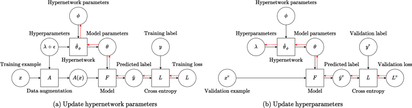
Figure 3: The computation graph of the HBA algorithm. (a) We train a hypernetwork, which represents a population of models, to minimize the training loss (Equation 13). (b) We update the hyperparameters by minimizing the validation loss (Equation 11). The arrows in red represent the gradient flow in the backward propagation.

3.4 Weight Sharing across Models.

Weight sharing is a commonly-used strategy to promote cooperation in training multiple models. Therefore, it looks natural to consider applying a weight sharing strategy in our population-based training. Recall that the update step (Equation 1) independently updates each model in the population. If some of the layers are shared among the population, the population members can be seen as performing a joint training in the update step. As we can see from the example in Figure 2 (c), if we share the weights of the linear layer, these two models, trained with different hyperparameters, learn different convolutional features while sharing the same linear classifier.

Besides model cooperation, another reason that motivates us to apply weight sharing is based on the following observation: applying a weight sharing strategy to the population is equivalent to adopting a simplified hypernetwork architecture, which can effectively reduce both the search time and memory consumption.

For example, if all the population members share a particular layer’s parameters, then it equivalently means that the corresponding hyper-layer degenerates into a constant function independent of hyperparameters. In other words, if we share a layer’s parameters, there is no need to associate it with a hyper-layer. By doing so, the number of hyper-layers becomes smaller, the memory consumption in the training process is reduced, and the search speed becomes faster. Taking Figure 2 (d) as an example, if we simultaneously employ a hypernetwork and shares the linear layer, then only the conv layer is attached with a hyper-conv layer. The hyper-linear layer degenerates into a constant function and thus is removed, giving us a smaller hypernetwork than the one without weight sharing (Figure 2 (b)). In summary, Figure 2 shows the corresponding model architectures of whether employing a hypernetwork and whether applying a weight sharing strategy.

3.5 Gradient-based Exploitation

With hypernetwork $\hat{\theta}_{\phi}$, the exploit step (Equation 4) can be modified accordingly as

$$k=\arg\min_{i\in\{1,...,n\}}\sum_{(x^{v},y^{v})\in D_{V}}\mathcal{L}(\mathcal{F}(x^{v};\hat{\theta}_{\phi}(\lambda_{i})),y^{v}).$$ (9)

However, a hypernetwork, as a continuous function, naturally represents not only $n$ models but also a continuous population of models. Therefore, we propose to find the best performing model $\hat{\theta}_{\phi}(\lambda^{*})$ in the continuous population by minimizing the validation loss over hyperparameters as

$$\lambda^{*}=\arg\min_{\lambda}\sum_{(x^{v},y^{v})\in D_{V}}\mathcal{L}(\mathcal{F}(x^{v};\hat{\theta}_{\phi}(\lambda)),y^{v}).$$ (10)

We use gradient descent to approximately yet efficiently find $\lambda^{*}$. In particular, our exploit step is changed as applying $T_{val}$ steps of SGD to solve Equation 10, and each step can be written as

$$\lambda=\lambda-\alpha^{\prime}\frac{1}{n}\sum_{i=1}^{n}\nabla_{\lambda}\mathcal{L}(\mathcal{F}(x^{v}_{i},\hat{\theta}_{\phi}(\lambda)),y^{v}_{i}).$$ (11)

Explore and Update. Based on Equation 11, the explore step of $\lambda_{i}$ (Equation 5) can be modified accordingly as

$$\lambda_{i}=\lambda+\epsilon_{i}.$$ (12)

Besides, we let the model parameters be implicitly exploited and explored by $\theta_{i}=\hat{\theta}_{\phi}(\lambda_{i})=\hat{\theta}_{\phi}(\lambda+\epsilon_{i})$, which can be seen as an approximation of $\hat{\theta}_{\phi}(\lambda)+\epsilon^{\prime}_{i}$.

Furthermore, by substituting Equation 12 into Equation 8, we merge the explore and update step together and obtain the formula of updating the hypernetwork as

$$\phi=\phi-\alpha\frac{1}{n}\sum_{i=1}^{n}\nabla_{\phi}\mathcal{L}(\mathcal{F}(\mathcal{A}(x_{i};\lambda+\epsilon_{i});\hat{\theta}_{\phi}(\lambda+\epsilon_{i})),y_{i}).$$ (13)

where $\epsilon_{i}\sim N(0,\sigma)$. Lastly, instead of using the same perturbation noise $\{\epsilon_{i}\}_{i=1}^{n}$ across the $T_{train}$ SGD steps of Equation 13, we re-sample $\{\epsilon_{i}\}_{i=1}^{n}$ for each iteration to enhance the sample diversity. In other words, at each SGD step, we sample a different discrete set of models from the continuous population to update the hypernetwork.

Summary. Algorithm 1 summarizes our HBA algorithm, which is a gradient-based training algorithm that alternates between updating the hypernetwork (Equation 13) and updating the hyperparameters (Equation 11). HBA builds upon the concept of the population-based training (Equation 1 to 6) while performs a gradient-based training (Equation 11 and 13). In Figure 3, we show the computation graph of the HBA algorithm.

Algorithm 1 The algorithm of HBA.

1:  Input: training set $D_{T}$, validation set $D_{V}$, model network $\mathcal{F}(\cdot;\theta)$, hypernetwork $\hat{\theta}_{\phi}$, augmentation policy $\mathcal{A}(\cdot;\lambda)$, batch size $n$, number of steps $T$, $T_{train}$ and $T_{val}$, learning rates $\alpha$ and $\alpha^{\prime}$, standard deviation $\sigma$.

2:  Initialize $\phi$ and $\lambda$

3:  for $j=1$ to $T$ do

4:     for $t=1$ to $T_{train}$ do

5:        Sample $\{(x_{i},y_{i})\}_{i=1}^{n}$ from $D_{T}$

6:        $\{\epsilon_{i}\}_{i=1}^{n}\sim N(0,\sigma)$

7:        $\phi=\phi-\alpha\frac{1}{n}\sum_{i=1}^{n}\nabla_{\phi}\mathcal{L}(\mathcal{F}(\mathcal{A}(x_{i};\lambda+\epsilon_{i}),\hat{\theta}_{\phi}(\lambda+\epsilon_{i})),y_{i})$ $\triangleright$ Update $\phi$ (Equation 13)

8:     end for

9:     for $t=1$ to $T_{val}$ do

10:        Sample $\{(x^{v}_{i},y^{v}_{i})\}_{i=1}^{n}$ from $D_{V}$

11:        $\lambda=\lambda-\alpha^{\prime}\frac{1}{n}\sum_{i=1}^{n}\nabla_{\lambda}\mathcal{L}(\mathcal{F}(x^{v}_{i},\hat{\theta}_{\phi}(\lambda)),y^{v}_{i})$ $\triangleright$ Update $\lambda$ (Equation 11)

12:     end for

13:  end for

14:  Output: $\hat{\theta}_{\phi}(\lambda)$

4 Experiments

Implementation Details. Following STN [23], HBA trains the hypernetwork parameters using SGD with $T_{train}=2$ and optimizes the hyperparameters using Adam [15] with $T_{val}=1$. We implemented HBA using the Pytorch [25] framework. We measured the search time of HBA on an NVIDIA Tesla V100 GPU. We reported the last epoch’s performance after training for all of our results using the mean and standard deviation over five runs with different random seeds. For policy evaluation, we scaled the length of the discovered schedules linearly if necessary.

Search Space. We define a data augmentation policy as a stochastic transformation function constructed by a set of elementary image operations. Each operation is associated with a probability and a magnitude, which play the role of data augmentation hyperparameters. For a fair comparison in Section 4.1 and 4.2, our transformation function follows PBA [12], which consists of $15$ operations and performs three steps: (1) sampling an integer $K$ from a categorical distribution as the number of operations to be applied, where $K\sim$ {0: $p$ = 0.2, 1: $p$ = 0.3, 2: $p$ = 0.5}. (2) sampling $K$ operations based on the operation probabilities, and (3) sequentially applying these sampled operations to the input image. Figure 4 (b) lists the $15$ operations, whose detailed description can be found in the supplementary material.

4.1 Ablation Study

	CIFAR-10	CIFAR-100	GPU
Strategy	Val. Error (%)	Val. Error (%)	Hours
Conv + BN	$2.85\pm 0.13$	$19.15\pm 0.21$	$7.74$
Conv	$2.88\pm 0.06$	$19.18\pm 0.26$	$6.85$
BN	$2.74\pm 0.05$	$19.18\pm 0.34$	$4.23$
1st Conv	$2.81\pm 0.07$	$19.39\pm 0.25$	$\mathbf{3.36}$
1st BN	$\mathbf{2.72}\pm 0.12$	$\mathbf{18.80}\pm 0.34$	$3.37$

Table 2: Ablation study on different weight sharing strategies.

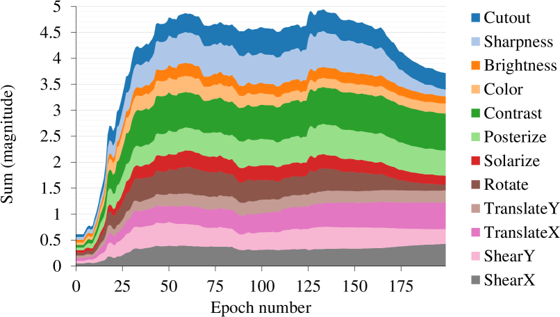
(a) Operation magnitudes

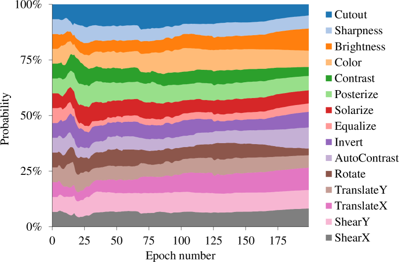
(b) Normalized probabilities

Figure 4: The learned hyperparameter schedule of data augmentation. (a) In terms of the operation magnitudes, their sum is rapidly increased initially and slowly decreased at the end. (b) Our schedule is smoothly-varying in terms of the probabilities. The ratio of the largest to the smallest probability is about $5$ during the training.

Weight Sharing Strategy. We first conducted an ablation study on different weight sharing strategies. In general, if we share a subset of the trainable layers’ parameters from the perspective of population-based training, it means that we do not associate them with hyper-layers. We experimented with five weight sharing strategies: Conv+BN, Conv, BN, 1st Conv, and 1st BN. These strategies are named by what layers are added with hyper-layers. For example, the Conv strategy means that we add HyperConv layers to all the convolutional layers and ignore the other layers. The 1st BN strategy means that we only add a HyperBN layer to the lowest BN layer.

The intuition behind our weight sharing strategies is as follows. For the low-level layers, we do not share parameters so that they are enforced to reflect the influence of different augmentation policies. For the mid- and high-level layers, we share parameters to encourage the population to learn a joint feature representation.

In this study, we split the CIFAR training set into three sets (30k/10k/10k) and denoted them as Train30k/Val0/Val. The CIFAR test set was not used in this study. For policy search, we applied HBA to train Wide-ResNet-28-10 (WRN-28-10) [33] on the Train30k/Val0 split to find policies. For policy evaluation, we used the searched policies to train networks on the Train30k+Val0 set and evaluated them on the Val set.

Table 10 shows the comparison results between these five strategies. We can see that adding fewer hyper-layers reduces search time and achieves slightly better performance across different datasets, showing that weight sharing in population-based training is helpful in the manner of model cooperation. We also experimented with WRN-40-2 and obtained similar results, which are included in the supplementary material. Based on the ablation results, we employ the 1st BN strategy in the subsequent experiments unless otherwise mentioned.

Standard Deviation $\sigma$ for exploration. Next, we analyzed $\sigma$ in Equation 13, representing the range of exploration. Similar to the previous experiment, we train WRN-28-10 on CIFAR-10. Three values of $\sigma$ are experimented: $0.5$, $1.0$, and $2.0$, which yield Val set errors of $3.43\pm 0.09\%$, $3.30\pm 0.10\%$, and $3.38\pm 0.05\%$, respectively. Based on the results, we used $\sigma=1.0$ in all of our experiments.

Method	CIFAR-10	SVHN	ImageNet
AA [5]	5000	1000	15000
PBA [12]	5	1	-
FAA [20]	3.5	1.5	450
OHLAA [21]	83.4	-	625
AdvAA [35]	-	-	1280
DADA [19]	0.1	0.1	1.3
HBA	0.1	0.1	0.9

Table 3: Comparison of search time in GPU hours. HBA has the least search time and is competitive to DADA.

	Baseline	Cutout	AA	PBA	FAA	OHLAA	RA	AdvAA	DADA	HBA
CIFAR-10
Wide-ResNet-40-2	$5.3$	$4.1$	$3.7$	-	$3.6$	-	-	$3.6$	-	$3.80\pm 0.15$
Wide-ResNet-28-10	$3.9$	$3.1$	$2.6$	$2.6$	$2.7$	-	$2.7$	$1.9$	$2.7$	$2.63\pm 0.10$
Shake-Shake (26 2x32d)	$3.6$	$3.0$	$2.5$	$2.5$	$2.7$	-	-	$2.4$	$2.7$	$2.63\pm 0.16$
Shake-Shake (26 2x96d)	$2.9$	$2.6$	$2.0$	$2.0$	$2.0$	-	$2.0$	$1.9$	$2.0$	$2.03\pm 0.10$
Shake-Shake (26 2x112d)	$2.8$	$2.6$	$1.9$	$2.0$	$2.0$	-	-	$1.8$	$2.0$	$1.97\pm 0.05$
PyramidNetN+ShakeDrop	$2.7$	$2.3$	$1.5$	$1.5$	$1.8$	-	$1.7$	$1.4$	$1.7$	$1.58\pm 0.06$
CIFAR-100
Wide-ResNet-40-2	$26.0$	$25.2$	$20.7$	-	$20.7$	-	-	-	$20.9$	$20.60\pm 0.37$
Wide-ResNet-28-10	$18.8$	$18.4$	$17.1$	$16.7$	$17.3$	-	$16.7$	$15.5$	$17.5$	$17.46\pm 0.48$
Shake-Shake (26 2x96d)	$17.1$	$16.0$	$14.3$	$15.3$	$14.9$	-	-	$14.1$	$15.3$	$15.35\pm 0.38$
PyramidNetN+ShakeDrop	$14.0$	$12.2$	$10.7$	$10.9$	$11.9$	-	-	$10.4$	$11.2$	$12.10\pm 0.14$
SVHN
Wide-ResNet-28-10	$1.5$	$1.3$	$1.1$	$1.2$	$1.1$	-	$1.0$	-	$1.2$	$1.11\pm 0.02$
Shake-Shake (26 2x96d)	$1.4$	$1.2$	$1.0$	$1.1$	-	-	-	-	$1.1$	$1.05\pm 0.03$
ImageNet
ResNet-50 (top-1 error)	$23.7$	-	$22.4$	-	$22.4$	21.1	$22.4$	$20.6$	$22.5$	$22.11\pm 0.10$
ResNet-50 (top-5 error)	$6.9$	-	$6.2$	-	$6.3$	5.7	$6.2$	$5.5$	$6.5$	$6.17\pm 0.05$

Table 4: The test set error rates $(\%)$ on CIFAR-10, CIFAR-100, SVHN, and ImageNet.

4.2 Automated Data Augmentation

We compare HBA with standard augmentation (Baseline), Cutout [8], AutoAugment (AA) [5], Population Based Augmentation (PBA) [12], Fast AutoAugment (FAA) [20], OHL-Auto-Aug (OHLAA) [21], RandAugment (RA) [6], Adversarial AutoAugment (AdvAA) [35], and Differentiable Automatic Data Augmentation (DADA) [19]. Except for Baseline and Cutout, all the methods adopt an AutoAugment-like search space.

Settings. We evaluate HBA on four image classification datasets: CIFAR-10 [17], CIFAR-100 [17], SVHN [24], and ImageNet [7]. For each dataset, we randomly sampled a subset of 10,000 images from the original training set as the validation set $D_{V}$ for HBA. Following the experimental setting of [5, 12, 20], we randomly sampled a subset from the remaining images to create a reduced version of the training set. For policy search, we applied HBA to train a WRN-40-2 network on the reduced datasets. For policy evaluation, we evaluated the performance of a model $M$ by using the searched policy to train $M$ on the original training set and measuring the accuracy on the test set. Please see the supplementary material for the detailed settings.

CIFAR-10 and CIFAR-100. The CIFAR-10 and CIFAR-100 datasets consist of 60,000 natural images, with a size of 32x32. The training and test sets have 50,000 and 10,000 images, respectively. We applied our augmentation policy, baseline, and Cutout (with 16x16 pixels) in sequence to each training image. The baseline augmentation is defined as the following operations in sequence: standardization, horizontal flipping, and random cropping. We evaluated our searched policies with WRN-40-2, WRN-28-10, Shake-Shake [9], and PyramidNet+ShakeDrop [30]. As shown in Table 3 and 4, HBA significantly improves the performance over the baseline and Cutout, while achieving competitive accuracy with the compared methods. HBA only takes $0.2$ GPU hours on the Reduced CIFAR-10 for policy search, which is an order of magnitude faster than PBA (population-based) and is comparable to DADA (gradient-based). In Figure 4, we visualize the discovered augmentation policy with WRN-40-20 on the CIFAR-10 dataset.

SVHN. The SVHN dataset consists of 73,257 training images (called core training set), 531,131 additional training images, and 26,032 test images. We applied our augmentation policy, baseline, and Cutout (with 20x20 pixels) in sequence to each training image. The baseline augmentation applied standardization only. We evaluated our searched policies with WRN-40-2, WRN-28-10, and Shake-Shake. As shown in Table 3 and 4, HBA achieves competitive accuracy and slightly outperforms PBA and DADA.

ImageNet. The ImageNet dataset has a training set of about 1.2M images and a validation set of 50,000 images. We applied our augmentation policy and then the baseline augmentation to each training image. Following [20], the baseline augmentation applied random resized crop, horizontal flip, color jittering, PCA jittering, and standardization in sequence. We evaluated our searched policies with ResNet-50 [11]. As shown in Table 3 and 4, HBA is at least three orders of magnitude faster than all the compared methods except DADA. Compared with DADA, HBA achieves higher accuracy.

Policy Search			Policy Evaluation
Dataset	Model	Time (GPU hours)	Dataset	Model	Test Error (%)
Reduced CIFAR-10	WRN-40-2	$0.1$	CIFAR-10	WRN-40-2	$3.78\pm 0.15$
			CIFAR-100		$20.58\pm 0.37$
			CIFAR-10	WRN-28-10	$2.63\pm 0.10$
			CIFAR-100		$17.46\pm 0.48$
CIFAR-10	WRN-40-2	$1.2\uparrow$	CIFAR-10	WRN-40-2	$3.63\pm 0.07\downarrow$
CIFAR-100			CIFAR-100		$20.80\pm 0.28\uparrow$
CIFAR-10	WRN-28-10	$4.5\uparrow$	CIFAR-10	WRN-28-10	$2.59\pm 0.09\downarrow$
CIFAR-100			CIFAR-100		$16.87\pm 0.22\downarrow$

Table 5: Comparison between policy search on the proxy task (top half) and the target tasks (bottom half).

Summary. Table 3 summarizes the comparison of search time. We can see that HBA has the least search time. Besides, we also compare with RandAugment (RA), which does not report its search time in its paper. RA performs a grid search, and its search time (in GPU hours) can be written as $NT$ where $N$ is the number of grid samples, and $T$ is the GPU hours of a single training run. $N$ is $15$ in its CIFAR-10 experiment. HBA’s search time is about $1.6T$, where $1.6$ is obtained from measuring the ratio of ”HBA’s training time” to ”the typical training time,” where both training is conducted on CIFAR-10 with WRN-40-2. Based on the above analysis, we can see that HBA requires much less GPU hours than RA.

HBA versus DADA. In terms of search time, HBA is comparable to DADA, which is the current state-of-the-art. Comparing with DADA on the accuracy, HBA achieves $3$ wins, $9$ ties, and $1$ loss, as shown in Table 4.

Policy Search on the Target Tasks. In the previous experiments (Table 3 and 4), we applied HBA on a reduced task, which trains a smaller network (WRN-40-2) on a reduced dataset. Here, we compared with the performance of policy searched on the target tasks, which trains the target network on the full dataset to find the augmentation policy. We consider training a model $M\in\{\text{WRN-40-2},\text{WRN-28-10}\}$ on a dataset $D\in\{\text{CIFAR-10},\text{CIFAR-100}\}$, giving us four target tasks. Table 5 shows that training on the target tasks requires longer search times while achieving slightly better performances (in three out of four cases), which is similar to the findings in RA [6] and DADA [19]. These results demonstrate that although HBA is designed to pursue efficiency, it can trade off search time for accuracy by searching on the target tasks.

HBA versus RandAugment. Although HBA requires fewer GPU hours than RA, HBA does not outperform RA in terms of accuracy. One may still prefer RA over HBA because of the extreme simplicity of grid search. We note that the AutoAugment search space is so well-designed that a reduced grid search could suffice. To address this concern and justify HBA’s effectiveness, our next experiment considers a different search space.

	Val. Loss	Test Loss	Test Error $(\%)$
GS	$0.794$	$0.809$	-
RS	$0.921$	$0.752$	-
STN	$0.579\pm 0.005$	$0.582\pm 0.004$	$19.86\pm 0.21$
HBA	$\mathbf{0.548\pm 0.005}$	$\mathbf{0.556\pm 0.005}$	$\mathbf{18.76\pm 0.11}$

Table 6: Comparison with grid search (GS), random search (RS), and STN on tuning regularization hyperparameters.

4.3 Comparison with STN

We followed the experiment settings of STN [23] and applied HBA to simultaneously train an AlexNet [18] on CIFAR-10 and tune regularization hyperparameters. Here, the search space consists of $15$ regularization hyperparameters: $7$ for data augmentation and $8$ for dropout. We employed the Conv strategy to construct our hypernetwork for the AlexNet model. As shown in Table 6, both gradient-based methods outperform grid search and random search. Besides, HBA performs better than STN, showing the effectiveness of our weight sharing strategy.

5 Conclusion

We proposed HBA, a gradient-based method for automated data augmentation. HBA employs a hypernetwork to train a continuous population of models and uses gradient descent to tune augmentation hyperparameters. Our weight sharing strategy improved both the search speed and accuracy. Future directions include applying HBA to different domains such as medical images and exploring hybrid algorithms that interpolate between PBT and HBA.

Appendix A Search space

Elementary Image Operations. Table 7 shows the list of augmentation operations used in our experiments except for Section 4.3. When applying an operation $op\in\{\text{ShearX},\text{ShearY},\text{TranslateX},\text{TranslateY},\text{Rotate}\}$ to an input image, we randomly negate the sampled magnitude with a probability of $0.5$.

Augmentation Function. Following PBA [12], we use a categorical distribution $K\sim~{}${0: $p$ = 0.2, 1: $p$ = 0.3, 2: $p$ = 0.5} as the number of operations to bee applied. Please refer to the Algorithm 1 in the PBA paper for the augmentation function used for both PBA and our HBA.

Initialization. For each augmentation hyperparameter, we initialize its value by $0.95M_{\text{min}}+0.05M_{\text{max}}$, where $[M_{\text{min}},M_{\text{max}}]$ is the magnitude range of the hyperparameter.

Implementation Details. Following PBA [12], our search space consists of $15$ operations, where each has two copies. We note that, unlike PBA that discretizes continuous hyperparameters, we treat all hyperparameters (both probabilities and magnitudes) as continuous variables. Following STN [23], we define the hyperparameters $\lambda$ as the unbounded version of the operation magnitudes and probabilities by mapping a range of magnitude $[M_{\text{min}},M_{\text{max}}]$ to $[-\infty,\infty]$ through a logit function (the inverse of the sigmoid function). The magnitude range of each operation is shown in Table 7, and the probability range of each operation is $[0,1]$.

Table 7: List of augmentation operations.

Operation	Range of Magnitude	Unit of Magnitude
ShearX	[0, 0.3]	-
ShearY	[0, 0.3]	-
TranslateX	[0, 0.45]	Image size
TranslateY	[0, 0.45]	Image size
Rotate	[0, 30]	Degree
AutoContrast	None	-
Invert	None	-
Equalize	None	-
Solarize	[0, 255]	-
Posterize	[0, 8]	Bit
Contrast	[0.1, 1.9]	-
Color	[0.1, 1.9]	-
Brightness	[0.1, 1.9]	-
Sharpness	[0.1, 1.9]	-
Cutout	[0, 0.2]	Image size

Appendix B Population-Based Training Procedure

Our population-based training procedure can be expressed in the format of PBT [14] as follows:

Step: each model runs an SGD step with a batch size of $1$.

Eval: we evaluate each model on a validation set by cross entropy loss.

Ready: each model goes through the exploit-and-explore process every $T_{train}$ steps.

Exploit: each model clones the weights and hyperparameters of the best performing model.

Explore: for each model, we perturb the value of its parameters and hyperparameters.

Algorithm 2 Our population-based training procedure.

1:  Input: population size $n$, number of steps $T$ and $T_{train}$, training set $D_{T}$, augmentation policy $\mathcal{A}$, neural network $\mathcal{F}$, learning rate $\alpha$, validation set $D_{V}$, Gaussian sigma $\sigma$ and $\sigma^{\prime}$.

2:  Initialize $\{\theta_{i}\}_{i=1}^{n}$ and $\{\lambda_{i}\}_{i=1}^{n}$

3:  for $j=1$ to $T$ do

4:     for $i=1$ to $n$ (synchronously in parallel) do

5:        for $t=1$ to $T_{train}$ do

6:           // Step

7:           Sample $(x,y)$ from $D_{T}$

8:           $\theta_{i}=\theta_{i}-\alpha\nabla_{\theta}\mathcal{L}(\mathcal{F}(\mathcal{A}(x;\lambda_{i});\theta_{i}),y)$

9:        end for

10:     end for

11:     // Eval

12:     $k=\arg\min_{i\in\{1,...,n\}}$ $~{}~{}~{}~{}~{}~{}~{}\sum_{(x^{v},y^{v})\in D_{V}}\mathcal{L}(\mathcal{F}(x^{v};\theta_{i}),y^{v})$

13:     // Exploit

14:     for $i=1$ to $n$ do

15:        $\lambda_{i}=\lambda_{k}$

16:        $\theta_{i}=\theta_{k}$

17:     end for

18:     // Explore

19:     for $i=1$ to $n$ do

20:        $\lambda_{i}=\lambda_{i}+\epsilon_{i}$ where $\epsilon_{i}\sim N(0,\sigma)$

21:        $\theta_{i}=\theta_{i}+\epsilon^{\prime}_{i}$ where $\epsilon^{\prime}_{i}\sim N(0,\sigma^{\prime})$

22:     end for

23:  end for

24:  Output: $\theta_{k}$

Appendix C Implementation Details of Hyper-layers

C.1 Hyper-Linear Layer

Let $f$ be a linear layer. We have

$$y=f(x;W)=Wx,$$ (14)

where $x\in\mathbb{R}^{c_{1}}$, $y\in\mathbb{R}^{c_{2}}$, and the weight matrix $W\in\mathbb{R}^{c_{2}\times c_{1}}$ is the parameters of the linear layer. Given a linear layer $f$, we define its corresponding Hyper-linear layer $\hat{W}$ as a linear function that maps hyperparameters $\lambda\in\mathbb{R}^{n}$ to the weight matrix $W\in\mathbb{R}^{c_{2}\times c_{1}}$ of the linear layer $f$. We can decompose the hyperlinear layer $\hat{W}$ into a set linear functions $\{\hat{w}_{i}(\lambda)\}_{i=1}^{c_{2}}$ that each function $\hat{w}_{i}(\lambda)$ outputs the transpose of the i-th row of $W$. $\hat{W}$ can be expressed as

$$W=\hat{W}(\lambda) =[\hat{w}_{1}(\lambda),...,\hat{w}_{c_{2}}(\lambda)]^{T}$$ (15)

$$\text{and~{}~{}}\hat{w}_{i}(\lambda) =w_{i}+A_{i}\lambda,$$ (16)

where $A_{i}\in\mathbb{R}^{c_{1}\times n}$ and $w_{i}\in\mathbb{R}^{c_{1}}$. A Hyper-linear layer parameterized by $\{A_{i}\}_{i=1}^{c_{2}}$ and $\{w_{i}\}_{i=1}^{c_{2}}$ requires $nc_{1}c_{2}$ and $c_{1}c_{2}$ parameters, respectively. Due to its prohibitively huge memory consumption, following Self-Tuning Network (STN) [23], we assume $A_{i}$ is a rank-$1$ matrix to greatly reduce the number of parameters of the Hyper-linear layer. Specifically, we define $A_{i}=u_{i}v_{i}^{T}$ where $u_{i}\in\mathbb{R}^{c_{1}}$ and $v_{i}\in\mathbb{R}^{n}$. By doing so, the number of parameters of the Hyper-linear layer is reduced to $(n+c_{1})c_{2}+c_{1}c_{2}$. $\hat{w}_{i}(\lambda)$ is written as

$$\hat{w}_{i}(\lambda) =w_{i}+A_{i}\lambda=w_{i}+u_{i}v_{i}^{T}\lambda=w_{i}+(v_{i}^{T}\lambda)u_{i}.$$ (17)

The Hyper-linear layer $\hat{W}(\lambda)$ can then be expressed as

$$W=\hat{W}(\lambda) =[\hat{w}_{1}(\lambda),...,\hat{w}_{c_{2}}(\lambda)]^{T}$$ (18)

$$=W_{0}+\text{diag}(V\lambda)U$$ (19)

where $W_{0}=[w_{1},...,w_{c_{2}}]^{T}\in\mathbb{R}^{c_{2}\times c_{1}}$, $V=[v_{1},...,v_{c_{2}}]^{T}\in\mathbb{R}^{c_{2}\times n}$, $U=[u_{1},...,u_{c_{2}}]^{T}\in\mathbb{R}^{c_{2}\times c_{1}}$, and $\text{diag}(\cdot)$ turns a vector into a diagonal matrix. In particular, $W$, $W_{0}$, and $U$ have the same matrix size. Let $W_{0}$, $U$, and $V$ be denoted by $\phi_{0}$, $\phi_{U}$, and $\phi_{V}$, respectively. The hyper-linear layer can be expressed in a general form as

$$W=\hat{W}(\lambda;\phi_{0},\phi_{U},\phi_{V})=\phi_{0}+\text{diag}(\phi_{V}\lambda)\phi_{U}.$$ (20)

Consider a linear layer with a bias $\bm{b}$, the bias part of the hyperLinear layer can be additionally defined in a similar way as

$$b=\hat{b}(\lambda;\phi_{0}^{\text{b}},\phi_{U}^{\text{b}},\phi_{V}^{\text{b}})=\phi_{0}^{\text{b}}+\text{diag}(\phi_{V}^{\text{b}}\lambda)\phi_{U}^{\text{b}}$$ (21)

where $\phi_{0}^{\text{b}}\in\mathbb{R}^{c_{2}}$, $\phi_{V}^{\text{b}}\in\mathbb{R}^{c_{2}\times n}$, and $\phi_{U}^{\text{b}}\in\mathbb{R}^{c_{2}}$.

C.2 Hyper-Conv Layer

A linear layer can be interpreted as a $1\times 1$ convolutional layer by (1) viewing the input vector $x$ as an image with $c_{1}$ channels and a spatial size of $1\times 1$, and (2) viewing the weight matrix $W$ as the set of $1\times 1$ convolutional filters, where each row of $W$ is a filter. Therefore, we can define the hyper-layer of a $1\times 1$ convolutional layer in the same way as the hyper-linear layer. We follow the definition of the hyper-linear layer (Equation 20), and define the hyper-conv1x1 layer as

$$\theta_{\text{conv1x1}} =\hat{\theta}_{\text{conv1x1}}(\lambda;\phi_{0}^{\text{c}},\phi_{U}^{\text{c}},\phi_{V}^{\text{c}})$$ (22)

$$=\phi_{0}^{\text{c}}+\text{diag}(\phi_{V}^{\text{c}}\lambda)\phi_{U}^{\text{c}},$$ (23)

where $\theta_{\text{conv1x1}},\phi_{0}^{\text{c}},\phi_{U}^{\text{c}}\in\mathbb{R}^{c_{2}\times c_{1}}$ are three sets of $1\times 1$ filters. $c_{1}$ and $c_{2}$ are the number of the input and output channels, respectively. $\text{diag}(\phi_{V}^{\text{c}}\lambda)\phi_{U}^{\text{c}}$ can be interpreted as a filter-wise scaling of $\phi_{U}^{\text{c}}$, in which the j-th filter weights of $\phi_{U}^{\text{c}}$ are scaled by the j-th element of $\phi_{V}^{\text{c}}\lambda$. In general, the hyper-conv layer for a $k\times k$ convolutional layer can be defined with the hyper-conv1x1 layer by changing $\phi_{0}^{\text{c}}$ and $\phi_{U}^{\text{c}}$ from $1\times 1$ to $k\times k$ filters as follows:

$$\theta_{\text{conv}}=\hat{\theta}_{\text{conv}}(\lambda;\phi_{0}^{\text{c}},\phi_{U}^{\text{c}},\phi_{V}^{\text{c}})=\phi_{0}^{\text{c}}+\text{diag}(\phi_{V}^{\text{c}}\lambda)\phi_{U}^{\text{c}},$$ (24)

where each row of $\phi_{0}^{\text{c}}$ and $\phi_{U}^{\text{c}}$ corresponds to the parameters of a $k\times k$ filter. Specifically, $\theta_{\text{conv}},\phi_{0}^{\text{c}},\phi_{U}^{\text{c}}\in\mathbb{R}^{c_{2}\times c_{1}k^{2}}$, $\phi_{V}^{\text{c}}\in\mathbb{R}^{c_{2}\times n}$. For a Conv layer with a bias, the bias part of the hyper-conv layer is the same as the hyper-linear one (Equation 21).

C.3 Hyper-BN Layer

A batch normalization layer has a trainable affine transformation. Following the design spirit of the hyper-linear and the hyper-conv layer, we denote the affine parameters by $\theta_{\text{BN}}$ and define the hyper-BN layer as

$$\theta_{\text{BN}} =\text{hyper-BN}(\lambda;\phi_{0}^{\text{BN}},\phi_{U}^{\text{BN}},\phi_{V}^{\text{BN}})$$ (25)

$$=\phi_{0}^{\text{BN}}+\text{diag}(\phi_{V}^{\text{BN}}\lambda)\phi_{U}^{\text{BN}},$$ (26)

where $\phi_{0}^{\text{BN}}\in\mathbb{R}^{2c_{2}}$, $\phi_{V}^{\text{BN}}\in\mathbb{R}^{2c_{2}\times n}$, $\phi_{U}^{\text{BN}}\in\mathbb{R}^{2c_{2}}$, and $c_{2}$ is the number of the output channels. There is a factor $2$ because the affine transformation has $c_{2}$ scaling parameters and $c_{2}$ offset parameters.

Appendix D Hyperparameters

Table 8 and 9 show the hyperparameters used in policy search and policy evaluation, respectively. For the ImageNet dataset, we used a step-decay learning rate schedule that drops by $0.1$ at epoch $90$, $180$, and $240$.

Dataset	Reduced CIFAR-10	Reduced SVHN	Reduced ImageNet	CIFAR-10 / CIFAR-100
No. classes	10	10	120	10
No. training images	4,000	4,000	6,000	40,000
No. validation images	10,000	10,000	10,000	10,000
Model	WRN-40-2	WRN-40-2	WRN-40-2	WRN-40-2 / WRN-28-10
Input size	32x32	32x32	32x32	32x32
No. training epoch	200	160	270	200
Learning rate $\alpha$	$0.05$	$0.01$	$0.1$	$0.1$
Learning rate schedule ($\alpha$)	cosine	cosine	step	cosine
Weight decay	$0.005$	$0.01$	$0.001$	$0.0005$
Batch size	128	128	128	128
Learning rate $\alpha^{\prime}$	$0.03$	$0.02$	$0.007$	$0.003$
Learning rate schedule ($\alpha^{\prime}$)	constant	constant	constant	constant
Results in the main paper	Table 4	Table 4	Table 4	Table 5

Table 8: Hyperparameters for policy search.

Dataset	Model	LR	Schedule	WD	BS	Epoch
CIFAR-10	WRN-40-2	0.1	cosine	0.0005	128	200
CIFAR-10	WRN-28-10	0.1	cosine	0.0005	128	200
CIFAR-10	Shake-Shake (26 2x32d)	0.01	cosine	0.001	128	1800
CIFAR-10	Shake-Shake (26 2x96d)	0.01	cosine	0.001	128	1800
CIFAR-10	Shake-Shake (26 2x112d)	0.01	cosine	0.001	128	1800
CIFAR-10	PyramidNet+ShakeDrop	0.05	cosine	0.00005	64	1800
CIFAR-100	WRN-28-10	0.1	cosine	0.0005	128	200
CIFAR-100	Shake-Shake (26 2x96d)	0.01	cosine	0.0025	128	1800
CIFAR-100	PyramidNet+ShakeDrop	0.025	cosine	0.0005	64	1800
SVHN	WRN-28-10	0.005	cosine	0.001	128	160
SVHN	Shake-Shake (26 2x96d)	0.01	cosine	0.00015	128	160
ImageNet	ResNet-50	0.1	step	0.0001	256	270

Table 9: Hyperparameters for policy evaluation. LR: learning rate. Schedule: learning rate schedule. WD: weight decay. BS: batch size. Epoch: number of training epoch. All the hyperparameters follow the settings in PBA [12] except the ones for the ImageNet dataset. We used $8$ NVIDIA Tesla V100 GPUs to train ResNet-50 on the ImageNet dataset.

Appendix E Ablation study of weight sharing strategies.

In Table 10, we show the full results of the ablation study on weight sharing strategies. In particular, we experimented with both Wide-ResNet-40-2 and Wide-ResNet-28-10. Their results are consistent: adding fewer hyper-layers reduces search time and achieves slightly better performance.

	Wide-ResNet-40-2			WideResNet-28-10
Hyper-layers	CIFAR-10	CIFAR-100	Time	CIFAR-10	CIFAR-100	Time
	Val. Error (%)	Val. Error (%)	(GPU Hours)	Val. Error (%)	Val. Error (%)	(GPU Hours)
Conv + BN	$4.01\pm 0.09$	$22.66\pm 0.19$	$2.03$	$2.85\pm 0.13$	$19.15\pm 0.21$	$7.74$
Conv	$3.94\pm 0.08$	$22.71\pm 0.34$	$1.53$	$2.88\pm 0.06$	$19.18\pm 0.26$	$6.85$
BN	$3.86\pm 0.08$	$22.86\pm 0.22$	$1.33$	$2.74\pm 0.05$	$19.18\pm 0.34$	$4.23$
1st Conv	$\mathbf{3.85}\pm 0.06$	$22.66\pm 0.40$	$\mathbf{0.86}$	$2.81\pm 0.07$	$19.39\pm 0.25$	$\mathbf{3.36}$
1st BN	$4.02\pm 0.11$	$\mathbf{22.20}\pm 0.10$	$0.87$	$\mathbf{2.72}\pm 0.12$	$\mathbf{18.80}\pm 0.34$	$3.37$

Table 10: Ablation study on different weight sharing strategies.

References

- [1] Gabriel Bender, Pieter-Jan Kindermans, Barret Zoph, Vijay Vasudevan, and Quoc Le. Understanding and simplifying one-shot architecture search. In ICML, 2018.
- [2] David Berthelot, Nicholas Carlini, Ian Goodfellow, Nicolas Papernot, Avital Oliver, and Colin A Raffel. MixMatch: A holistic approach to semi-supervised learning. In Advances in Neural Information Processing Systems, pages 5050–5060, 2019.
- [3] Andrew Brock, Theodore Lim, James M Ritchie, and Nick Weston. SMASH: one-shot model architecture search through hypernetworks. In ICLR, 2018.
- [4] Ting Chen, Simon Kornblith, Mohammad Norouzi, and Geoffrey Hinton. A simple framework for contrastive learning of visual representations. In ICML, 2020.
- [5] Ekin D Cubuk, Barret Zoph, Dandelion Mane, Vijay Vasudevan, and Quoc V Le. AutoAugment: Learning augmentation strategies from data. In CVPR, 2019.
- [6] Ekin D Cubuk, Barret Zoph, Jonathon Shlens, and Quoc V Le. RandAugment: Practical automated data augmentation with a reduced search space. In NeurIPS, 2020.
- [7] Jia Deng, Wei Dong, Richard Socher, Li-Jia Li, Kai Li, and Li Fei-Fei. ImageNet: A large-scale hierarchical image database. In CVPR, 2009.
- [8] Terrance DeVries and Graham W Taylor. Improved regularization of convolutional neural networks with cutout. arXiv preprint arXiv:1708.04552, 2017.
- [9] Xavier Gastaldi. Shake-shake regularization. In ICLR, 2017.
- [10] David Ha, Andrew Dai, and Quoc V Le. Hypernetworks. In ICLR, 2017.
- [11] Kaiming He, Xiangyu Zhang, Shaoqing Ren, and Jian Sun. Deep residual learning for image recognition. In CVPR, 2016.
- [12] Daniel Ho, Eric Liang, Ion Stoica, Pieter Abbeel, and Xi Chen. Population based augmentation: Efficient learning of augmentation policy schedules. In ICML, 2019.
- [13] Sergey Ioffe and Christian Szegedy. Batch normalization: Accelerating deep network training by reducing internal covariate shift. In ICML, 2015.
- [14] Max Jaderberg, Valentin Dalibard, Simon Osindero, Wojciech M Czarnecki, Jeff Donahue, Ali Razavi, Oriol Vinyals, Tim Green, Iain Dunning, Karen Simonyan, et al. Population based training of neural networks. arXiv preprint arXiv:1711.09846, 2017.
- [15] Diederick P Kingma and Jimmy Ba. Adam: A method for stochastic optimization. In ICLR, 2015.
- [16] Ilya Kostrikov, Denis Yarats, and Rob Fergus. Image augmentation is all you need: Regularizing deep reinforcement learning from pixels. In ICLR, 2021.
- [17] Alex Krizhevsky and Geoffrey Hinton. Learning multiple layers of features from tiny images. Technical Report, 2009.
- [18] Alex Krizhevsky, Ilya Sutskever, and Geoffrey E Hinton. Imagenet classification with deep convolutional neural networks. In Advances in neural information processing systems, 2012.
- [19] Yonggang Li, Guosheng Hu, Yongtao Wang, Timothy M. Hospedales, Neil Martin Robertson, and Yongxin Yang. DADA: differentiable automatic data augmentation. In ECCV, 2020.
- [20] Sungbin Lim, Ildoo Kim, Taesup Kim, Chiheon Kim, and Sungwoong Kim. Fast AutoAugment. In NeurIPS, 2019.
- [21] Chen Lin, Minghao Guo, Chuming Li, Xin Yuan, Wei Wu, Junjie Yan, Dahua Lin, and Wanli Ouyang. Online hyper-parameter learning for auto-augmentation strategy. In ICCV, 2019.
- [22] Hanxiao Liu, Karen Simonyan, and Yiming Yang. DARTS: Differentiable architecture search. In ICLR, 2019.
- [23] Matthew MacKay, Paul Vicol, Jon Lorraine, David Duvenaud, and Roger Grosse. Self-tuning networks: Bilevel optimization of hyperparameters using structured best-response functions. In ICLR, 2019.
- [24] Yuval Netzer, Tao Wang, Adam Coates, Alessandro Bissacco, Bo Wu, and Andrew Y. Ng. Reading digits in natural images with unsupervised feature learning. In NIPS Workshop on Deep Learning and Unsupervised Feature Learning 2011, 2011.
- [25] Adam Paszke, Sam Gross, Francisco Massa, Adam Lerer, James Bradbury, Gregory Chanan, Trevor Killeen, Zeming Lin, Natalia Gimelshein, Luca Antiga, et al. PyTorch: An imperative style, high-performance deep learning library. In Advances in Neural Information Processing Systems, 2019.
- [26] Hieu Pham, Melody Y Guan, Barret Zoph, Quoc V Le, and Jeff Dean. Efficient neural architecture search via parameter sharing. In ICML, 2018.
- [27] Connor Shorten and Taghi M Khoshgoftaar. A survey on image data augmentation for deep learning. Journal of Big Data, 2019.
- [28] Nitish Srivastava, Geoffrey Hinton, Alex Krizhevsky, Ilya Sutskever, and Ruslan Salakhutdinov. Dropout: a simple way to prevent neural networks from overfitting. JMLR, 2014.
- [29] Qizhe Xie, Zihang Dai, Eduard Hovy, Minh-Thang Luong, and Quoc V Le. Unsupervised data augmentation for consistency training. In NeurIPS, 2020.
- [30] Yoshihiro Yamada, Masakazu Iwamura, Takuya Akiba, and Koichi Kise. Shakedrop regularization for deep residual learning. IEEE Access, 2019.
- [31] Tong Yu and Hong Zhu. Hyper-parameter optimization: A review of algorithms and applications. arXiv preprint arXiv:2003.05689, 2020.
- [32] Sangdoo Yun, Dongyoon Han, Seong Joon Oh, Sanghyuk Chun, Junsuk Choe, and Youngjoon Yoo. CutMix: Regularization strategy to train strong classifiers with localizable features. In ICCV, 2019.
- [33] Sergey Zagoruyko and Nikos Komodakis. Wide residual networks. In BMVC, 2016.
- [34] Hongyi Zhang, Moustapha Cisse, Yann N Dauphin, and David Lopez-Paz. mixup: Beyond empirical risk minimization. In ICLR, 2018.
- [35] Xinyu Zhang, Qiang Wang, Jian Zhang, and Zhao Zhong. Adversarial AutoAugment. In ICLR, 2020.
- [36] Barret Zoph and Quoc V Le. Neural architecture search with reinforcement learning. In ICLR, 2017.