Innovation and Imitation

Abstract.

We study several models of growth driven by innovation and imitation by a continuum of firms, focusing on the interaction between the two. We first investigate a model on a technology ladder where innovation and imitation combine to generate a balanced growth path (BGP) with compact support, and with productivity distributions for firms that are truncated power-laws. We start with a simple model where firms can adopt technologies of other firms with higher productivities according to exogenous probabilities. We then study the case where the adoption probabilities depend on the probability distribution of productivities at each time. We finally consider models with a finite number of firms, which by construction have firm productivity distributions with bounded support. Stochastic imitation and innovation can make the distance of the productivity frontier to the lowest productivity level fluctuate, and this distance can occasionally become large. Alternatively, if we fix the length of the support of the productivity distribution because firms too far from the frontier cannot survive, the number of firms can fluctuate randomly.

1. Introduction

Economic growth is partly the result of costly research activities that firms undertake in order to innovate, and to increase their productivity. Growth is also driven by technology diffusion and imitation that takes place between firms. The role of technology diffusion across countries is evidenced by the extraordinary sustained growth rates in China and other East Asian countries during the recent decades. In this paper we investigate several models of growth driven both by innovation and imitation, focusing on the interaction between the two. New ideas and innovations push out the technology frontier. Imitation enables firms to catch up with those higher up on the technology ladder. We study the dynamics of the productivity distribution of firms, where productivity is increasing with the rates of innovation and imitation, and we provide a characterization of its stationary distribution in the long run. In our study we do not take into account the effect of the size of the firm on its growth.

As demonstrated by Lucas (2009), in models of technology diffusion based on imitation alone, growth can be sustained only if the initial distribution of productivities has unbounded support for high productivity levels. In Lucas and Moll (2014), and Perla and Tonetti (2014), technology diffusion is search theoretic, where firms seek higher productivity firms to imitate from and to adopt superior technology. In these models an unbounded productivity distribution is necessary to sustain growth through imitation in the long run. With an initial productivity distribution that has bounded support imitation ultimately stops, as productivities of the imitating firms collapse toward the productivity frontier. Therefore, unboundedness is more than a convenient and inconsequential simplification.

In contrast, in models of endogenous growth, innovation is the primary driving force of growth. Firms engage in research to generate individual innovations. These innovations later may become a common stock of ideas that are available to the whole economy, generating spillovers (Romer (1990)). Alternatively, innovations are Schumpeterian, in the sense that firms can leapfrog beyond the productivity frontier. They overtake incumbent firms and drive them out of business, increasing overall productivity over time (Aghion and Howitt (1992)).

Models involving both random innovations via a geometric Brownian motion, as well as imitation via random meetings between firms generating technology diffusion, have been proposed by Luttmer (2012) and Staley (2011). Their approach is related to the KPP equation, originally studied in the mathematics literature by Kolmogorov, Petrovski and Piskunov (1937), and later by McKean (1975) and Bramson (1984) among others. These models can admit a unique balanced growth path (BGP) that is a global attractor, and whose shape depends on imitation and innovation propensities, but not on initial conditions. Innovations driven by Brownian motion however assures that the productivity distribution immediately becomes unbounded, and the resulting BGP does not have compact support.

Having a compact support is particularly relevant for empirical purposes, as the support of the productivity distribution in individual industries is found to be quite localized (Syverson (2004), Hsieh and Klenow (2009)). Firms with significantly low productivity relative to the frontier firms are unlikely to survive the competition, and to preserve their market shares for long. The forces of Schumpeterian “creative destruction” may endogenously replace the inefficient firms at the bottom of the productivity distribution. However other firms, below but not too far from the frontier may survive, giving a distribution of productivities that allows both for innovation and imitation to persist over time.

In section 2, we first investigate a model on a ladder. Innovation and imitation combine to generate a balanced growth path (BGP) with compact support. In contrast to models with imitation alone (see Lucas (2009)), the distribution does not collapse to the frontier either. The distribution of productivities is centered around some productivity moving up at a constant growth rate, and keeps its shape relative to this productivity over time (a traveling wave which is compactly supported). In section 2.1 we first propose a very simple model of firms on a quality ladder that can both innovate and imitate, and where with some positive probability imitators can leapfrog to the productivity frontier. We characterize the stationary distribution of productivities as a truncated power law. This model has the advantage of being very simple, but leaves imitation rates mostly exogenous. In section 2.2 we extend this model to introduce density dependent imitation rates. In section 3 we endogenize the length of the support of balance growth path as arising from optimal choices of firms.

Another approach to generating productivity distributions that have finite support is to limit the number of firms to be finite. By construction, distributions over a finite number of firms have bounded support; however, stochastic imitation and innovation can make the distance of the productivity frontier to the lowest productivity level fluctuate, and this distance can occasionally become quite large. In section 4, we study such models with innovation, imitation and a finite number of firms, the so-called $N$-BRW and $L$-BRW models. These models introduce alternative approaches to modeling entry, exit, and competition, but also feature balanced growth paths with compact support. We characterize some features of their productivity distributions and relate them to results obtained in earlier sections. Section 5 concludes.

2. Innovation and imitation with fixed compact support

In this section, we consider a discrete time model of innovation and imitation. Innovation can be gradual, by moving up a quality ladder as in Klette and Kortum (2004) and König, Lorenz and Zillibotti (2016). But it can also be a breakthrough, where agents or firms move up from the bottom and overtake the top, that is they “leapfrog”. On top of that, agents imitate other agents. So we start in section 2.1 with a model of exogenous imitation rates. In section 2.2, we endogenize the imitation choice and obtain a stationnary productivity distribution that looks like a truncated power law on a finite support. Then in section 3 we show that the assumption of a fixed support length of the BGP is actually the result of an optimal choice problem that trades off the costs of imitation and its benefits, as in Perla and Tonetti (2014).

In this section, we only consider the case where the number of firms is sufficiently large to neglect finite-size effects and stochastic behavior. In fact, to make “microscopic” and probabilistic interpretations at the firm level, and not only speak about densities, we have to assume that a law of large number holds.

2.1. Exogenous innovation and imitation

At each time $t\in\mathbb{N}$, a firm has a productivity level $i\in\mathbb{N}$ on a discrete ladder.

The density of firms at time $t$ on level $i$ is given by a non-negative number $f_{t}^{i}\in\mathbb{R}_{+}^{0}$ with $\sum_{i}f_{t}^{i}=1$ for every $t$. At each time step, when going from $t$ to $t+1$, firms improve their productivity and the density climbs up the ladder along some rules which we explicit now. We assume that, at each time step and at each level, a fraction $a\in(0,1)$ of firms moves up the productivity ladder by one level (“innovation”), and a fraction $1-a$ remains stagnant, with the same productivity. This amounts to assuming a law of large numbers for random innovation with probability of success $a$. Then, all of the firms that remained stagnant at the lowest productivity level $i=1$ either leapfrog or imitate as described below, leaving the lowest level empty. (This corresponds to a fraction $(1-a)f_{t}^{1}$ of all firms.)

We call $m\in\mathbb{N}$ the highest level at time $t$. Given our process, at time $t+1$, the productivity level $i=m+1$ gets populated, and the lowest productivity level $i=1$ is emptied as described below. Then, at each period, we rename the levels: what was the level $i$ at time $t$ becomes the level $i-1$ at time $t+1$. In this way, the populated levels at the beginning of each time step are always numbered $\{1,2,\ldots,m\}$. For the moment, we take the length of support $m$ as given, and postpone a discussion of endogenously chosen $m$ to section 3.

In this section 2.1, imitation for non-innovating firms at the lowest level happens as follows: at level $i\in\{1,2,\ldots,m\}$, the fraction of imitators entering level $i$ at time $t+1$ is $(1-a)f_{t}^{1}q_{i}$, where the $q_{i}\in[0,1]$ satisfy

(1) $$q_{i}\geq 0,\qquad\sum_{i=1}^{m}q_{i}=1.$$

The $q_{i}$ for $i\in\{1,\ldots,m-1\}$ represent imitation (exogenous in this section 2.1), while $q_{m}$ represents leapfrogging — i.e. firms at the lowest level of the productivity distribution at each time $t$ that overtake the current productivity frontier (indeed, the productivity level $m$ at time $t+1$ corresponds to the productivity level $m+1$ at time $t$ which was not yet populated). If $q_{m}=0$, leapfrogging is excluded, while setting $q_{m}=1$ excludes any imitation.

Note that we assume that jumps to higher productivity levels, whether from leapfrogging or imitation, do not depend on target productivity densities, so for the time being we abstract away from any search-theoretic microfoundation.

The transition dynamics can be written in a single equation

(2) $$f_{t+1}^{i}=\underbrace{(1-a)f_{t}^{i+1}}_{\text{fall back}}+\underbrace{af_{t}^{i}}_{\text{innovation}}+\underbrace{(1-a)f_{t}^{1}q_{i}}_{\text{imitation or leapfrogging}}$$

or, more conveniently, with a matrix $A\in M_{m}([0,1])$ representing the productivity dynamics:

$$f_{t+1} =Af_{t}\ ,$$

(21) $$\left[\begin{array}[]{c}f_{t+1}^{1}\\ f_{t+1}^{2}\\ .\\ .\\ .\\ f_{t+1}^{m}\end{array}\right] =\left[\begin{array}[]{cccccc}a+q_{1}(1-a)&1-a&0&.&.&0\\ q_{2}\left(1-a\right)&a&1-a&0&.&.\\ .&.&.&.&.&.\\ .&.&.&a&1-a&0\\ q_{m-1}\left(1-a\right)&.&.&0&a&1-a\\ q_{m}\left(1-a\right)&0&.&.&0&a\end{array}\right]\left[\begin{array}[]{c}f_{t}^{1}\\ f_{t}^{2}\\ .\\ .\\ .\\ f_{t}^{m}\end{array}\right]\ .$$

By construction $A$ has column sums adding to $1$ as the number of firms remains constant (in effect, we have a particular birth and death model). $A$ admits $1$ as an eigenvalue. The associated eigenvector is the stationary distribution for productivity densities, moving up as a traveling wave. The stationary distribution can be characterized as follows.

Proposition 1.

Let $Q_{s}=\left(q_{m}+q_{m-1}+\cdots+q_{s}\right)=\sum_{j=s}^{m}q_{j}$, with $Q_{m}=q_{m}$ and $Q_{1}=1$.

The stationary distribution $\left(f_{\infty}^{1},f_{\infty}^{2},\ldots,f_{\infty}^{m}\right)$, for any $a\in(0,1)$, is given by:

(22) $$f_{\infty}^{s}=Q_{s}f_{\infty}^{1}\ ,s=1,...,m\ ,$$

and

$$f_{\infty}^{1}\left(\sum\limits_{s=1}^{m}Q_{s}\right)=1\ or\ \ f_{\infty}^{1}=\left(\sum\limits_{s=1}^{m}Q_{s}\right)^{-1}\ .$$

Proof.

The stationary solution fulfills $f_{\infty}=Af_{\infty}$. To simplify notation let $f_{\infty}^{j}\equiv x_{j},$ $j=1,\ldots,m$.

We start with the last line of equation (21):

$$q_{m}\left(1-a\right)x_{1}+ax_{m}=x_{m}\qquad\Rightarrow\qquad x_{m}=q_{m}x_{1}\ .$$

We prove by induction. The line next to last yields

$$q_{m-1}\left(1-a\right)x_{1}+ax_{m-1}+(1-a)x_{m}=x_{m-1}$$

$$\qquad\Rightarrow\left(q_{m-1}+q_{m}\right)\left(1-a\right)x_{1}=\left(1-a\right)x_{m-1}$$

$$\qquad\Rightarrow x_{m-1}=\left(q_{m-1}+q_{m}\right)x_{1}\ .$$

Assume that $x_{m-(s-1)}=(q_{m-(s-1)}+\cdots+q_{m})x_{1}$ . Then we have

$$q_{m-s}\left(1-a\right)x_{1}+ax_{m-s}+\left(1-a\right)x_{m-(s-1)}=x_{m-s}$$

$$\qquad\Rightarrow x_{m-s}=\left(q_{m-s}+q_{m-(s-1)}+\cdots+q_{m-1}+q_{m}\right)x_{1}\ .$$

This completes the induction proof. Relabeling $m-s$ as $s$, we obtain (22).

We have left one free variable, $x_{1}$, which will be determined by the normalization of $f$; writing $\sum_{i=1}^{m}x_{i}=1=x_{1}\left(\sum_{s=0}^{m-1}Q_{m-s}\right)=x_{1}\left(\sum_{s=1}^{m}Q_{s}\right)$, we get the results. ∎

The stationary distribution is independent of the probability of innovation $a\in(0,1),$ and only depends on the intensity $q_{i}$ of imitation rates across productivities. But the speed of convergence to the stationary distribution depends on $a$, as it affects the eigenvalues of $A$. In particular the second highest eigenvalue of $A$, which is less than $1$ in modulus, can be taken as an indicator of the convergence rate. The lower this eigenvalue, the faster the convergence rate. For $m=2$, it can be explicitly computed to be equal to $2a-1+q_{1}(1-a)=a-(1-a)q_{2}$. This is increasing in $q_{1}$ (more imitation implies slower convergence), decreasing in $q_{2}$, the leapfrogging rate (more leapfrogging implies faster convergence), and increasing in $a$ (more innovation implies slower convergence).

Firms at any productivity level except the lowest one tend to drop down the ladder over time. At the bottom of the ladder, non-innovating firms jump to higher levels through innovation and imitation. Overall, the stationary density of productivity levels is non-increasing over productivity levels.

We now discuss two special cases:

No imitation, only leapfrogging

If there is no imitation and only leapfrogging, that is if $q_{m}=1$ and therefore $q_{i}=0$ for $i\in\{1,\ldots,m-1\}$, it follows that $f_{\infty}^{i}=m^{-1}$ for $i=1,\ldots,m$, so the productivity distribution becomes uniform. Firms that jump to the frontier slide down the productivity distribution, until they reach the lowest density from which they again jump to the frontier.

No leapfrogging, only imitation

In this case $q_{m}=0$ and the matrix in (21) is decomposable. In particular, the highest productivity evolves with $f_{t+1}^{m}=af_{t}^{m}$ independently, and converges to zero. This makes the last element of the eigenvector associated with root $1$ equal to zero, so there is no density for it at the stationary distribution: $f_{\infty}^{m}=0$.

2.2. Density dependent imitation

In Proposition 1 we solved for the densities in terms of exogenous imitation rates $q_{i},$ $i=1,\ldots,m-1,$ with $m>2$. Now we consider the case that the imitation rates are proportional to densities. We are again seeking a stationary solution.

If imitation is similar to learning from another firm, then imitation rates should be proportional to the number of firms to learn from, or the density at the corresponding ladder point. Learning is then conditional on meeting another firm with higher productivity, which happens with a probability proportional to the density there. Therefore, we let imitation rates be

(23) $$q_{j}\equiv q_{j}^{t}=\mu f_{t}^{j+1}\ ,\ j=1,\ldots,m-1\ .$$

(Recall that $q_{j}$ is the probability of jumping to site $j$ at time $t+1$, which is the same as site $j+1$ at time $t$ because of the relabeling at each time step; this is why $q_{j}$ is proportional to $f_{t}^{j+1}$ and not $f_{t}^{j}$.) Here, $\mu$, which is determined by normalization, is time-dependent: as seen below, it can be written as a function of $f_{t}^{1}$. The highest $f_{t+1}^{m}$ is not imitated because it is not available for for imitation yet, so $q_{m}$, which represents leapfrogging, is independent of the densities, as in section 2.1. Observe that the problem is now non-linear, so existence and uniqueness of a solution are more involved than in the linear case. A stationary solution is again $f_{\infty}=A(f_{\infty})f_{\infty}$.

We first determine $\mu$: with $m$ fixed, we must have

(24) $$1=f_{t}^{1}+\cdots+f_{t}^{m}$$

and

(25) $$1=q_{1}+q_{2}+\cdots+q_{m}\ .$$

Therefore, in order to find a solution, $\mu$ cannot take arbitrary values but will be determined (together with $f_{\infty}$) as a function of $q_{m}$. Indeed, inserting (23) into (25), and using (24) we obtain:

(26) $$1=q_{m}+\mu\sum_{j=1}^{m-1}f_{t}^{j+1}=q_{m}+\mu(1-f_{t}^{1})\ .$$

This implies that, assuming that $f_{t}^{1}<1$

(27) $$\mu\equiv\mu_{t}=\frac{1-q_{m}}{1-f_{t}^{1}}\ .$$

Overall, in this subsection, the two parameters $m$ and $q_{m}$ determine all other quantities, including $\mu$. Note that the reason for which we are not free to choose $\mu$ is that we insist, in our model, that the lowest occupied site be emptied at each time step. This condition leads to (25) and then to (27). In section 4, we briefly discuss a model where $\mu$ is an arbitrary parameter and the lowest occupied site is not necessarily emptied at each time step.

For the stationary solution, we write $x_{j}=f_{\infty}^{j}$ as before and

(28) $$\mu=\frac{1-q_{m}}{1-x_{1}}\ .$$

Remark 1.

$x_{1}=1$ is never a solution. If $x_{1}=1$, $x_{j}=0$, $\forall j=2,\ldots,m$. Then, either $q_{m}=1$ and $q_{j}=0$, $\forall j=1,\ldots,m-1$, in which case the last line of (21) reads $x_{m}=(1-a)q_{m}x_{1}=0$. For $a<1$, this is only possible if $q_{m}=0$, a contradiction. Or, if $q_{m}<1$, $\mu=\infty$ and the problem is not well-defined.

Proposition 2.

Under the assumptions above, with $q_{m}\in\left(0,1\right)$,

(29) $$x_{i}=q_{m}x_{1}\left(1+\frac{1-q_{m}}{1-x_{1}}x_{1}\right)^{m-i}\ ,\qquad i=1,\ldots,m,\$$

where $x_{1}\in[0,1)$ is the unique solution to

(30) $$1=q_{m}\left(1+\frac{1-q_{m}}{1-x_{1}}x_{1}\right)^{m-1}\ ,$$

or

(31) $$x_{1}=\frac{(q_{m})^{-\frac{1}{m-1}}-1}{(q_{m})^{-\frac{1}{m-1}}-q_{m}}\ .$$

Proof.

We give a recursive proof. The last line of (21) gives again $x_{m}=q_{m}x_{1}$. Replacing $q_{i}=\mu x_{i+1}$ for $i=1$ to $m-1$ in (21), we again proceed by induction and assume that (29) holds for $i=m-(j-1)$. Then

$$x_{m-j} =x_{m-(j-1)}+q_{m-j}x_{1}=x_{m-(j-1)}(1+\mu x_{1})$$

$$\Rightarrow x_{m-j} =x_{m}(1+\mu x_{1})^{j}=q_{m}x_{1}\left(1+\mu x_{1}\right)^{j}\ .$$

This finishes the induction proof. Relabeling $i=m-j$, we obtain (29).

For existence of a solution, we need that

(32) $$x_{1}=(1+\mu x_{1})^{m-1}q_{m}x_{1}$$

or

(33) $$(1+\mu x_{1})^{m-1}q_{m}=1\ .$$

Inserting the expression for $\mu$, (28), this gives equation (30). Let us check that the solution thus obtained is normalized; we have

$$\sum_{i=1}^{m}x_{i}=\sum_{j=0}^{m-1}(1+\mu x_{1})^{j}q_{m}x_{1}=\frac{(1+\mu x_{1})^{m}-1}{(1+\mu x_{1})-1}q_{m}x_{1}=\frac{(1+\mu x_{1})-q_{m}}{\mu}\ ,$$

where we have also used (33). But according to equation (28), one has $\mu=1+\mu x_{1}-q_{m}$, and so we conclude that

$$\sum_{i=1}^{m}x_{i}=1$$

Therefore, a solution to (33) with $\mu$ given by (28) gives rise to a normalized $x$, as summed up in equation (30). Inserting the expression (31) for $x_{1}$ proves existence of a solution. This finishes the proof of Proposition 2. ∎

Corollary 1.

If $q_{m}=0$, there is no stationary solution.

Proof.

For $q_{m}=0$, we have $x_{m}=0$. Using equation (21), this implies that

(34) $$x_{m-1}=\mu 0x_{1}+(1-a)0+ax_{m-1}\ ,$$

which implies that $x_{m-1}=0$ for $a<1$. By recursion, $x_{j}=0$ $\forall j$, and there is no solution. ∎

While there is no stationary solution for $q_{m}=0$, the limit of the dynamics may nevertheless converge to a distribution with $x_{1}\to 1$ and $x_{i}\to 0$ for $i>1$. Recall that $\{x_{i}\}=\{1,0,0,\ldots\}$ is not a stationary state, because it would lead to $\mu=0$ and a ill-defined model. This case is easily illustrated for $m=2$.

Example 1.

Dynamics for $m=2$, $q_{2}=0$. We start from a density $f_{0}$ with $f^{1}_{0}=1-f^{2}_{0}$ and $f^{2}_{0}>0$ (else, as already pointed out, we would have $\mu\rightarrow\infty$). Then the dynamics for $f^{2}_{t}$ reduce to

$$f^{2}_{t+1}=af^{2}_{t}$$

and hence

$$f^{2}_{t}=f^{2}_{0}a^{t}\to 0\quad\text{as $t\to\infty$}\ .$$

By normalization,

$$f^{1}_{t}=1-f^{2}_{t}=1-f^{2}_{0}a^{t}\to 1\quad\text{as $t\to\infty$}$$

We can observe that because $q_{m}=0$, the upper level of the density is falling over time as only a fraction $a$, namely the innovators, remains there each period. In the general case, all upper levels will successively experience such a decline in population. Because imitation is proportional to the number of firms present at the productivity level, fewer and fewer firms will flow into the higher steps of the ladder, which will be successively depopulated. In the limit, a single ladder step survives.

We would not think that the problematic asymptotic behavior for $q_{m}=0$ is a major drawback of this model. Surely there are some highly innovative firms who leapfrog to the highest operational productivity levels, so that the case $q_{m}=0$ may be economically less interesting.

Example 2.

We provide numerical illustrations for the stationary densities for $m=10$ and $q_{m}\in\left\{0.1\,;\,0.3\,;\,0.5\,;\,0.99\right\}$. The solutions for $\mu$ and $x_{1}$ are

$$\begin{cases}\mu=1.1915,\quad x_{1}=0.2447&\text{if }q_{m}=0.1\\ \mu=0.8431,\quad x_{1}=0.1698&\text{if }q_{m}=0.3\\ \mu=0.5801,\quad x_{1}=0.1380&\text{if }q_{m}=0.5\\ \mu=0.0111,\quad x_{1}=0.1005&\text{if }q_{m}=0.99\end{cases}$$

These values can be computed from $\mu=(q_{m})^{-\frac{1}{m-1}}-q_{m}$, which is obtained from (28) and (31).

Figure 1 plots the solution for $\left\{x_{i}\right\}_{i=1}^{m}$ for these four cases.

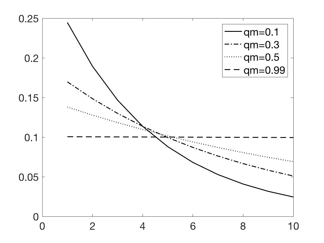
Figure 1. Stationary densities for different values of leapfrogging intensity $q_{m}$ with $m=10$.

Notice that higher values of $q_{m}$, or higher leapfrog values, flatten the productivity distribution. As $q_{m}\rightarrow 1,$ we have $\mu\rightarrow 0$ and $x_{i}\to m^{-1}$ for $i=1\,\ldots,m$, so the distribution is uniform. The stationary density gets increasingly concentrated at the lower boundary of the productivity ladder as $q_{m}$ gets smaller.

We note that in a continuous time version of this model with a continuum of firm productivities, with growth driven by imitation as well as by leap-frogging innovation to the frontier that is governed by a finite Markov chain, Benhabib, Perla and Tonetti (2017) also show that there exists a stationary productivity distribution evolving as a travelling wave with compact and bounded support.

3. Endogenizing the length of productivity distributions

In the previous section, only the firms at the lowest level $j=1$ would innovate or imitate at each time step. We now allow firms at any level $j\leq m$ to choose to leapfrog or imitate by paying a cost, if the firm estimates that it is profitable to do so. We first consider the simpler case of leapfrogging only (no imitation) in section 3.1, and we consider the full model with leapfrogging and imitation in section 3.2. In the first case (leapfrogging only, section 3.1), we will show that firms will only choose to leapfrog or imitate at or below a certain threshold level $j_{0}$ which is independent of time. Then with $j_{0}$ determined, the ladder length is fixed and given by $m-j_{0}+1$, and the results of section 2.1 with $q_{m}=1$ apply. In the second case (leapfrogging and imitation, section 3.2) we will also show that firms optimally choose to incur a cost for the opportunity to imitate or leapfrog at or below a certain threshold level $j_{0}(t)$, but this level might depend on time. In this case, characterizing the transition dynamics of the productivity distribution is not straightforward, but if we assume the system reaches a stationary distribution, then $j_{0}(t)$ converges to some $j_{0}(\infty)$ and the results of Proposition 2 in section 2.2 can be applied with the distribution of firms supported on an interval of size $m-j_{0}(\infty)+1$.

In either case, the finite size of the support is now endogenized and depends on what is the cost to imitate, what are the payoffs at each quality level, etc.

3.1. Leapfrogging Only

We assume that a firm still faces an exogenous probability of innovation $a$ as in sections 2.1 and 2.2 but, when the firm fails to innovate, it is allowed to make a choice to leapfrog (and pay some cost) or not. The firm’s optimal choice problem is to maximize its value function, i.e. the expected discounted value of current and future payoff streams net of costs. The firm’s choice is to choose for every period whether to pay a cost to leapfrog and benefit from higher payoffs now and in the future, or not to do so.

When evaluating if it is advantageous to take some action or not, a firm usually needs to anticipate the future distribution in order to have expectations for imitation probabilities and outcomes. In the case of leapfrogging only which we consider now, we will see that it is actually enough to know the position of the frontier $m=m(t)$, which remains constant (after relabeling) and equal to its initial position $m(0)$. (Without relabeling, we would have $m(t)=m(0)+t$ due to innovation.) Therefore, in the case of leapfrogging only, the outcome, when the firm decides whether to leapfrog or not, depends only on the initial value of $m$; it does not depend on the distribution of firms on the quality ladder, nor on time. (Note that this will no longer be true when we add imitation in section 3.2: with imitation, it is necessary to anticipate future distribution of firms to make an optimal choice.)

As is usual in economics, this optimal choice problem can be reformulated in a recursive way using a Bellman equation, that we will write down below. We will show here that the firm’s optimal choice is to leapfrog if it lies at a fixed length below the frontier. This fixed length becomes the new support size, thus providing a microfoundation to the previously exogenous support size $m$.

Every time step, at every level, a firm innovates and moves up one ladder step with probability $a$. The firms that do not innovate have the choice either to fall behind, or to catch up with the highest productivity level $m$ (after relabeling, or $m+1$ before) by paying a cost. We assume that it is not possible to “imitate” intermediate levels.

We assume that the payoffs realized by a given firm increase by some factor $\lambda>1$ each time the firm takes a step on the quality ladder, and we introduce the normalized payoffs $p_{j}=\lambda^{j}$ for a firm being at level $j\in\{1,\ldots,m\}$.

If, as the firm distribution moves up the quality ladder, costs to implement leap-frogging grow at the same rate $\lambda$ as the payoffs, the firm problem can be reduced to a stationary problem where the normalized payoffs $p_{j}=\lambda^{j}$ and the normalized cost $C$ are independent of time.

Firms, in deciding whether to leapfrog or not, compare the costs to the expected payoffs. As normalized payoffs increase over the ladder, while normalized costs do not, firms choose to leapfrog if their distance to the frontier (the level $m$ of the highest performing firm) is larger than some threshold, and choose not to leapfrog if their distance to the frontier is smaller than that threshold.

In other words, there must be a certain threshold level $j_{0}$ such that a firm chooses not to leapfrog for productivity levels $j=j_{0}+1,\ldots,m$, but does leapfrog at levels $j\leq j_{0}$. We now provide a formal argument.

Let $V_{\text{LF}}(j)$ be the value of leapfrogging from some level $j$ and $V_{\text{NLF}}(j)$ the value of not leapfrogging from this level. Then, the value of being at productivity level $j$ is

(35) $$V(j)=\max\big{\{}V_{\text{LF}}(j),V_{\text{NLF}}(j)\big{\}}\ .$$

The following equation represents the leapfrogging choice. We have

(36) $$V_{\text{LF}}(j) =p_{j}+\beta aV(j)+(1-a)\big{[}\beta V(m)-C\big{]},$$

where $\beta=\lambda\beta_{0}$, with $\beta_{0}<1$ the intertemporal discount factor; we assume that $\beta<1$. This is the Bellman equation for the leapfrogging value function, which determines the optimal choice recursively. The first term on the right-hand side is the payoff received this period. Then, with probability $a$, the firm innovates and moves up one step from $j$, which after relabeling becomes $j$, and this continuation value is discounted with $\beta$. With probability $(1-a)$, the firm does not innovate but decides to leapfrog; the firm moves above the frontier, at level $m+1$ (which after relabeling becomes level $m$) and pays the cost $C$.

Similarly,

(37) $$V_{\text{NLF}}(j)=p_{j}+\beta aV(j)+\beta(1-a)V(j-1).$$

Notice that neither (36) nor (37) depend on the densities $f$ or on time; the value $V(j)$ of being at some level $j$ remains constant in time.

The firm wants to leapfrog from some level $j$ if leapfrogging is beneficial, i.e.

(i) $$V_{\text{LF}}(j)>V_{\text{NLF}}(j)\ ,$$

and does not want to leapfrog if

(ii) $$V_{\text{LF}}(j)<V_{\text{NLF}}(j)\ .$$

Observe from (36) and (37) that

(38) $$V_{\text{LF}}(j)-V_{\text{NLF}}(j)=(1-a)\big{[}\beta V(m)-C-\beta V(j-1)\big{]}.$$

We assume from here on that the value function $V(j)$ increases with the productivity level $j$. This property is not an obvious consequence of Bellman’s equation, but it seems clear that any mathematical solution where $V(j)$ is not increasing cannot reasonably describe a real-life situation, because it would mean that some firms should degrade the quality of their production in order to increase their value.

Then, from (38) and using that $V(j)$ increases in $j$, the quantity $V_{\text{LF}}(j)-V_{\text{NLF}}(j)$ decreases with $j$. Hence, if leapfrogging is beneficial at $j$, it is even more so at $j-1$, $j-2$, etc. Similarly, if leapfrogging is not beneficial at $j$, it will be even less so at $j+1$, $j+2$, etc. In other words, there must be a threshold level $j_{0}$ such that

$$\text{A site leapfrogs if and only if }j\leq j_{0}.$$

Assume we let this system evolve from an initial condition where the highest occupied site is $m$. At the end of the first time step, site $m+1$ is occupied (through innovation and leapfrogging) and all sites up to and including $j_{0}$ are emptied through leapfrogging. At the start of the second time step, after relabeling, the system occupies a subset of sites $\{j_{0},\ldots,m\}$. Then, at each following time step, only site $j_{0}$ gets emptied through leapfrogging and the system remains in $\{j_{0},\ldots,m\}$ after relabeling. In the large time limit, the system reaches its stationary state, which is a uniform distribution over $\{j_{0},\ldots,m\}$.

This behavior we have just described is very similar to the behavior of the system in section 2.1 with $q_{m}=1$, except that the lowest occupied site is now $j_{0}$ instead of 1 in section 2.1. In other words, the size of the support is now $m-j_{0}+1$ instead of $m$. This size of support depends on the parameters of the model: $a$, $\lambda$, $C$ and $\beta$. (Using invariance by translation, it is easy to see that $m-j_{0}+1$ does not depend on $m$.) This means that the size of the support result from an endogenized optimum between costs and expected payoffs. By adjusting the values of the different parameters, any size of support can be obtained.

Through invariance by translation, one can shift the whole system on the value scale so that the support is on $\{1,\ldots,m^{\prime}=m-j_{0}+1\}$. Then, the model is even more similar to section 2.1 with $q_{m}=1$, with the lowest occupied level at $j=1$ and with the endogenized $m^{\prime}$ being both the highest occupied site and the size of the support.

3.2. Leapfrogging and imitation

We now introduce density-dependent imitation as in the section 2.2. A firm innovates at no cost with probability $a$ and, if it does not innovate, it can choose to pay a fixed cost $C$ to randomly leapfrog or imitate with density-dependent imitation probabilities, or it can forgo this opportunity. We are already assuming mean-field dynamics, which are valid in the limit of a large number of firms. We can therefore safely assume that the choice taken by a single firm does not impact the distribution.

Recall the following assumptions made in section 2.2: at time $t$, when a firm chooses to innovate or leapfrog, it jumps with probability $q_{j}$ ( with $j\in\{1,\ldots,m\}$) onto site $j+1$ which, after relabeling, becomes site $j$ at time $t+1$. Then, $q_{m}$ is the (exogenously given) probability of leapfrogging (since site $m+1$ is empty at time $t$) and $q_{j}$ for $j\leq m-1$ is the probability of imitating. We assume that for $j\leq m-1$, the probability of jumping on site $j+1$ (site $j$ after relabeling) is proportional to the proportion of firms $f_{t}^{j+1}$ on that site at the beginning of the time step, and we write $q_{j}=q_{j}(f)=(1-q_{m})f_{t}^{j+1}$ for $j\leq m-1$. The value of $1-q_{m}$ of the prefactor is chosen in such a way that the probabilities are normalized: $\sum_{j\leq m}q_{j}(f)=1$.

The value $V(j;f)$ of being at a site $j$ now depends on the density $\{f_{t}^{k}\}$ of firms at all sites for the current time. As in section 3.1, we write $V_{NLF}(j;f)$ for the value of being at $j$ and choosing not to imitate/leapfrog given the current densities $f=\left\{f^{k}\right\}$, and $V_{LF}(j;f)$ for the value of being at site $j$ and to imitate/leapfrog. The Bellman equations become

(39) $$V(j;f_{t}) =\max\Big{(}V_{NLF}(j;f_{t}),V_{LF}(j;f_{t})\Big{)},$$

(40) $$V_{NLF}(j;f_{t}) =p_{j}+\beta aV(j;f_{t+1})+\beta(1-a)V(j-1;f_{t+1}),$$

(41) $$V_{LF}(j;f_{t}) =p_{j}+\beta aV(j;f_{t+1})+(1-a)\bigg{(}\beta\sum_{k=j}^{m}q_{k}(f_{t})V(k;f_{t+1})$$

$$\hskip 156.49014pt+\beta\sum_{k<j}q_{k}(f_{t})V(j-1;f_{t+1})-C\bigg{)}$$

(42) $$=p_{j}+\beta aV(j;f_{t+1})+(1-a)\bigg{(}\beta V(j-1;f_{t+1})-C$$

$$\hskip 71.13188pt+\beta\sum_{k=j}^{m}q_{k}(f_{t})\big{[}V(k;f_{t+1})-V(j-1;f_{t+1})\big{]}\bigg{)}$$

(We assume that when it chooses to imitate/leapfrog, the firm first pays the price $C$. Then it selects a target to imitate with the probabilities $q_{k}$, but if that target is below its own quality, then the firm finally decides to not move. Recall that $p_{j}=\lambda^{j}$, $C$, and $\beta$ are normalized quantities (respectively payoffs, cost and discounting factor) as in the previous section. The second equality for $V_{LF}(j;f_{t})$ is obtained using $\sum_{k}q_{k}(f_{t})=1$.)

Notice that

$$V_{LF}(j;f_{t})-V_{NLF}(j;f_{t})=(1-a)\bigg{(}\beta\sum_{k=j}^{m}q_{k}(f)\big{[}V(k;f_{t+1})-V(j-1;f_{t+1})\big{]}-C\bigg{)}$$

and, then, that

$$\Big{[}V_{LF}(j;f_{t})-V_{NLF}(j;f_{t})\Big{]}-\Big{[}V_{LF}(j+1;f_{t})-V_{NLF}(j+1;f_{t})\Big{]}$$

$$\qquad\qquad\qquad=(1-a)\beta\bigg{(}\sum_{k=j}^{m}q_{k}(f_{t})\bigg{)}\big{[}V(j;f_{t+1})-V(j-1;f_{t+1})\big{]}$$

We assume, as in the previous section, that $V$ increases with $j$. Then $V_{LF}(j;f_{t})-V_{NLF}(j;f_{t})$ decreases with $j$. We conclude, as in section 3.1, that if imitaton or leapfrogging is advantageous at a given level $j$, it is even more advantageous at lower levels and that there must be, for each time $t$, a threshold level $j_{0}(t)$ such that a firm imitates or leapfrogs if $j\leq j_{0}(t)$ and does not otherwise.

Note that $j_{0}(t)$ depends on time because the values $V(k;f)$ and the jumping probabilities $q_{k}(f)$ depend on the densities $f$ which depend on time. In the stationary regime (assuming the system does reach a stationary regime), $j_{0}(t)=j_{0}$ becomes constant, the firms live in $\{j_{0},\ldots,m\}$ and only site $j_{0}$ decides to imitate or leapfrog. Therefore, the stationary regime is the same as the one described in section 2.2, but with an endogenized support size, $m-j_{0}+1$.

We have not discussed the case of separate choices for endogenous innovation and imitation, as analyzed by various authors, like Jovanovic and Rob (1989), Romer (1990), Aghion and Howitt (1992), Hoppenhyn (1992), Segestrom (1991), Klette and Kortum (2004), Luttmer (2007), Lucas and Moll (2014), Konig et al (2016), Benhabib, Perla and Tonetti (2014, 2017). In our ladder model with firms innovating from every level, separate costs might be chosen trivially such that firms always want to only innovate or only imitate.

4. Models with a finite number of firms: $N$-BRW and $L$-BRW

In the models presented in the previous sections, the quantity $f_{t}^{j}$ represented the fraction of firms with a quality $j$ at time $t$. If the market is made of $N$ firms, then the number of firms with quality $j$ at time $t$ should be around $Nf_{t}^{j}$. If $N\to\infty$, then the number of firms at a given quality is large for any $j$, the dynamics of the system is dominated by average quantities and the evolution is deterministic. All the models presented so far were assumed to be in this $N\to\infty$ limit. In this section, we explore the effect of having a large but finite number of firms $N$.

With a finite number of firms, the evolution of the system is intrinsically stochastic. Consider for instance a single site $j$ containing $n_{t}^{j}$ firms at time $t$, and assume each firm has a probability $a$ of innovating during one time step. Then, the number of firms innovating is a Binomial random number of parameters $n_{t}^{j}$ and $a$. On average, $an_{t}^{j}$ firms innovate with a standard deviation $[a(1-a)n_{t}^{j}]^{1/2}$. On productivity levels where $an_{t}^{j}\gg 1$, the fluctuations are negligible compared to the average behavior and stochasticity can be ignored. On the other hand, when $an_{t}^{j}$ is of order 1, the number of innovating firms is essentially random.

The models we consider in this section are stochastic versions of the model described in section 2.2. We still assume that firms live on a discrete quality ladder and that time is discrete. At the beginning of any time step, an active firm is characterized by its productivity level. Then, during one time step, for each firm, two things can happen (independently).

• The firm can innovate with probability $a$, thus gaining one productivity level.

• The firm can be imitated with probability $\mu$ by a new entrant.

The four outcomes for a single firm are graphically represented in figure 2.

Figure 2. The four outcomes after a time step for a single firm.

Note that in this section, and unlike in section 2, we do not rename the productivity levels after each time step and we assume that $\mu$ is a parameter given exogenously.

The evolution of the whole system during one time step then comes in two phases:

(43) $$\begin{cases}\text{(a)}&\text{each firm present at time $t$ evolves independently according}\\[-2.15277pt] &\text{to the probabilities in figure~{}\ref{outcomes},}\\ \text{(b)}&\text{a culling of the firms in the system occurs by removing}\\[-2.15277pt] &\text{some firms at the bottom of the productivity scale.}\end{cases}$$

Note that in the evolution phase, the imitating firms can either be some firms at the lowest productivity level who successfully imitate those above them, or new entrants displacing firms at the lowest level of productivity. There is no leapfrogging in this model.

We consider two variants of the model, depending on the way the culling occurs. A first variant is to fix the number of firms at each time step to an exogenous parameter $N$. Then, the number of removed firms during the culling phase must be equal to the number of imitated firms in the evolution phase to keep the total number of firms constant. This model is called a $N$-BRW ($N$ Branching Random Walk) and is discussed in section 4.1.

Another possibility for the culling phase is to remove all firms lagging $L$ productivity steps or more behind the most productive firm, with $L$ given exogenously. In this variant, the total number of firms fluctuate with time. This model is called a $L$-BRW ($L$ Branching Random Walk) and is discussed in section 4.2.

In the following sections we characterize the shape and properties of the productivity distributions in the $N$-BRW and $L$-BRW models of innovation and imitation. The discussion is adapted from works that have been conducted on KPP fronts since the late nineties in the context of statistical mechanics, reaction-diffusion models and population genetics. A good point of entry on this literature is Brunet (2016).

4.1. The $N$-BRW model

Before introducing the $N$-BRW, we need first to discuss what a BRW is. A Branching Random Walk is a process in discrete time started from a single particle at the origin. At each time step, each particle (each “parent”) is replaced by a random number of particles (the “children”) positioned relatively to the parent according to some point process. This rule is applied independently at each generation for each particle.

Figure 3. Left: an exemple of BRW where, at each generation a particle can have 1, 2 or 3 offsprings. Right: a $N$-BRW with $N=2$ obtained by keeping at each time step only the two highest children of the surviving particles of the previous time step. Notice that this rule is not the same as keeping the two highest particles of the BRW at each time step.

For instance, following figure 2, the rule could be that a particle at $y$ gives either one particle at $y$, or two particles at $y$, or one particle at $y+1$ or two particles respectively at $y$ and $y+1$. The left part of figure 3 shows a BRW with a different rule where each parent can have 1, 2 or 3 children.

Note that the number of particles $N_{t}$ at each generation follows the following recursion: $N_{t+1}=\sum_{i=1}^{N_{t}}n^{i,t}$, where $n^{i,t}$ is the number of children of individual $i$ at time $t$ and where it is assumed that the $n^{i,t}$ are independent identically distributed random variables over integers. This is called a Galton-Watson process. In other words, a BRW is a Galton-Watson process where we keep as an extra information the position of the particles. For simplicity, we exclude the possibility that a particle has zero children and we insist that it has more than one child with positive probability. Then, the population size increases exponentially with time.

Denote by $(\epsilon_{1},\epsilon_{2},\ldots,\epsilon_{n})$ the positions of the children relative to the parent (both $n$ and the $\epsilon_{i}$ are random). Then, under conditions on the laws of $n$ and $\epsilon_{i}$, listed for example in Gantert, Hu and Shi (2011) (see also there for references), one can show that the highest position $y_{\text{max}}(t)$ in the BRW at time $t$ increases linearly with time:

(44) $$\lim_{t\to\infty}\frac{y_{\text{max}}(t)}{t}=v_{c},$$

with some velocity $v_{c}$ given by

(45) $$v_{c}=\min_{\gamma}v(\gamma)=v(\gamma_{c})\qquad\text{with }v(\gamma)=\frac{1}{\gamma}\log\mathbb{E}\bigg{[}\sum_{i=1}^{n}e^{\gamma\epsilon_{i}}\bigg{]},$$

as soon as this minimum exists for some $\gamma_{c}>0$.

Here the expectation is both on the displacements $\epsilon_{i}$ and the number $n$ of children. $\gamma_{c}$ is the value of $\gamma$ for which the minimum is reached.

For instance, with the rules of figure 2, one checks that

$$v(\gamma)=\frac{1}{\gamma}\log\big{[}1+\mu+a(e^{\gamma}-1)\big{]}.$$

Indeed,

$$\mathbb{E}\Big{[}\sum_{i=1}^{n}e^{\gamma\epsilon_{i}}\Big{]} =(1-a)(1-\mu)\times e^{0}+(1-a)\mu\times(e^{0}+e^{0})$$

$$\quad\qquad+a(1-\mu)\times e^{\gamma}+a\mu\times(e^{0}+e^{\gamma})=1+\mu+a(e^{\gamma}-1)\ .$$

We can now define the $N$-BRW. The evolution for one time step of a $N$-BRW goes like a BRW, except that after each step only the $N$ highest particles are kept, the other being removed, so that after some time there are exactly $N$ particles in the system at each time step. Note that this rule is not the same as keeping the $N$ highest of a BRW at each time step; see the right part of figure 3.

The $N$-BRW and related models (the $N$-BBM, the stochastic Fisher equation) have been studied in mathematics, theoretical physics and biology and several results are known both from non-rigorous and rigorous arguments.

For the $N$-BRW, a striking result is that one can still define a velocity $v_{N}$ for the highest particle, as in (44). This velocity depends on $N$, converges to $v_{c}$ as $N\to\infty$, but the speed of convergence is unexpectedly slow (this is explained in Brunet and Derrida (1997) with a rigorous proof provided by Berard and Gouéré (2010) for the case $\mu=1$).

Theorem 1 (Velocity. Berard and Gouéré (2010)).

For the $N$-BRW with $\mu=1$, we have:

(46) $$v_{N}=v_{c}-\frac{\pi^{2}v^{\prime\prime}(\gamma_{c})}{2L_{0}^{2}}+o\left(\frac{1}{L_{0}^{2}}\right)$$

with

(47) $$L_{0}=\frac{1}{\gamma_{c}}\log N,$$

$v_{c}$, $v(\gamma)$ and $\gamma_{c}$ defined as in (45) and $o({1}/{L_{0}^{2}})$ a term that is vanishing faster than $1/L_{0}^{2}$ as $N\to\infty$ .

(Nota: even though a proof is available only in one case, heuristic arguments and numerical simulations suggest that (46) holds in a large number of cases.)

Size of support

Based on numerical observations and phenomenological theory for closely related models, it is believed (see Brunet and Derrida (1997) and Brunet, Derrida, Mueller and Munier (2006)) that after a long time, the system reaches a stationary regime as seen from the center of mass of the system. Here, stationary is to be interpreted in a probabilistic sense: while for finite $N$, there are still fluctuations, the laws determining the system become stationary. In this stationary regime, the size of support, which is the difference between the position $y_{\text{max}}$ of the highest particle and the position $y_{\text{min}}$ of the lowest particle, satisfies

(48) $$L:=y_{\text{max}}-y_{\text{min}}=L_{0}+\mathcal{O}(1),$$

with $L_{0}$ as in (47) and $\mathcal{O}(1)$ is designating a random variable whose law becomes independent of $N$ in the large $N$ limit. (Therefore, it will be smaller and smaller as compared to $L_{0}$ when $N\to\infty$.).

By construction, a finite number of firms assures a productivity distribution that has a finite support at any fixed time, but what (48) means is that the firms have at all time comparable productivity levels, and the scenario where some firms stay put while others diverge at infinity due to innovations cannot occur. However, because the process is stochastic, there is a probability of a firm with an extended streak of successful innovations breaking out for a while, so that the support of productivity distribution may occasionally get large, but after some time laggard firms will catch-up via imitation and close the gap.

Shape of the front

Another interesting result concerns the typical density of the cloud of particles in the stationary regime. To simplify the discussion, we assume that the underlying BRW is the one described in figure 2. Then, the population lives on the lattice, and we introduce $f(y,t)$ the fraction of particles (or firms) at position (or quality level) $y$ at time $t$.

After the reproduction phase (but before the culling phase, see (43)), the expected fraction of firms at position $y$ and time $t+1$ is $(1-a+\mu)f(y,t)+a\,f(y-1,t)$. Then, one could write the evolution equation as

(49) $$f(y,t+1)=(1-a+\mu)f(y,t)+a\,f(y-1,t)+(\text{noise})\quad\text{if $y>y_{\text{min}}(t+1)$}\ ,$$

where $y_{\text{min}}(t)$ is the position of the lowest firm at time $t$ (the values of $y_{\text{min}}(t+1)$ and of $f\big{(}y_{\text{min}}(t+1),t+1\big{)}$ are obtained by writing $\sum_{y}f(y,t+1)=1$). The noise term is some random number with zero expectation and standard deviation of order $\mathcal{O}(\sqrt{{f}/{N}})$, depending on the density.

As $N\to\infty$, in the so-called hydrodynamic limit, the noise term in (49) is expected to disappear. While there are no rigorous result concerning this hydrodynamic limit for the $N$-BRW, such a result exists for two closely related models, see Durrett and Remenik (2011) and De Masi, Ferrari, Presutti and Soprano-Loto (2019). In the first model, time is continuous, and at rate 1 each particle creates an additional particle at a random distance $\epsilon$; when this occurs, the lowest particle is removed to keep the population constant. The second model is the $N$-BBM, which can be described as follows: time and space are continuous. $N$ particles perform independent Brownian motions. At rate 1, each particle creates an offspring at its own position ($\epsilon=0$); when this occurs, the lowest particle is removed to keep the population constant.

The equation obtained in this large $N$ limit, as given by (49) without the noise term, is reminiscent of the model described in section 2.2. The only remaining difference is that in section 2.2, the imitation rate was tuned at each time step in such a way that $y_{\text{min}}(t)$ would increase by exactly one unit at each time step. In (49) (with or without the noise term), the imitation rate $\mu$ is fixed exogenously and, depending on its value, the lower bound $y_{\text{min}}(t)$ can increase by several units in a time step or take several time steps to increase by one unit.

The evolution equation is maybe easier to write on $h(y,t)=\sum_{z\geq y}f(z,t)$, which represents the fraction of firms with a quality level at least $y$. One checks that

(50) $$h(y,t+1)=\min\Big{[}1,(1-a+\mu)h(y,t)+a\,h(y-1,t)+(\text{noise})\Big{]}$$

where, here again, the noise term disappears in the large $N$ limit. Without the noise term, (50) is the discrete-time version of the equation studied in [8] which was shown to display most of the characteristics of the Fisher-KPP equation. With the noise term, it is very similar to the equations studied in Brunet and Derrida (1997), Brunet and Derrida (2001) and Brunet, Derrida, Mueller and Munier (2006) papers, as well as Mueller, Mytnik and Quastel (2011), which is with continuous time and space.

As suggested by Brunet and Derrida (1997), the velocity (46) of the noisy front (and thus of the $N$-BRW) could be obtained to the $1/L_{0}^{2}$ order by replacing the noise term in (50) by a cutoff of order $1/N$, meaning that after each time step the value of $h$ is set to 0 at all the positions $y$ where the evolution equation leads to a result smaller than $1/N$. Furthermore, the shape of the front at large times is for large $N$ (and hence large $L_{0}=(\log N)/\gamma_{c}$), large $z$ and large $L_{0}-z$ (so that $z$ is not too close to 0 or to $L_{0}$) approximately given by

(51) $$h(y_{\text{min}}(t)+z,t)\approx AL_{0}\sin\frac{\pi z}{L_{0}}\,e^{-\gamma_{c}z}\ .$$

Notice then that, to leading order, the density $f(y,t)=h(y,t)-h(y+1,t)$ is given by the same equation with the prefactor $A$ replaced by $A(1-e^{-\gamma_{c}})$ .

The shape of the front (51) is for the front equation (49) with the noise replaced by a cutoff. For the $N$-BRW model itself as described by equation (49) with its noise term, Brunet, Derrida, Munier and Muller (2006) give the following non-rigorous phenomenological description of the model. This description is supported by numerical simulation and, to some extent, by rigorous work (Maillard (2016)).

In the $N$-BRW, the shape of the front is most of the time given by the cutoff shape (51) plus some small fluctuations. Occasionally, typically every $\propto L_{0}^{3}$ units of time, a huge fluctuation occurs where the shape of the front is significantly different from (51) for about $\propto L_{0}^{2}$ units of time. Such a huge fluctuation comes in the following way: a single particle moves up further than typical (a single firm innovates a lot in a short time). That particle branches as usual (the firm is imitated), but its ‘imitation offspring’, i.e. its imitators, the imitators of its imitators, etc., are at first rarely removed from the system because they typically lie above the others (they have better quality than the other firms). The end effect of such a fluctuation is that a positive fraction of all the firms are replaced by the imitation offspring of the highly successful firm that started the fluctuation. So, to reformulate, based on numerical computations for similar models, in the stationary regime, a density of firms like (51) is expected, while occasionally (every $\propto L_{0}^{3}$ units of time), a single firm innovates a lot and gets imitated by so many firms that it redefines the industry (in the sense that the innovation is shared by a positive fraction of the agents). The transition time to redefine the industry is of order $\propto L_{0}^{2}$.

This is particularly interesting: at random times, a firm is so successful that a full fraction of the industry ends up imitating it (or its imitators).

A word of caution: the results presented above are asymptotic results, which are believed to be valid for large values of $N$. It is not obvious that $N=10^{4}$ or $N=10^{5}$ are big enough for these results to be very accurate.

4.2. The $L$-BRW model

A variant of the $N$-BRW is the $L$-BRW which might be more adapted to describe a situation where lagging firms go out of business and new firms enter the market. The evolution phase of the $L$-BRW (innovation and imitation) is the same as for the BRW or the $N$-BRW (particles innovate and are imitated), but the culling phase is different; in the $L$-BRW, at each time step, firms with a productivity lagging more than $L$ level below the leading firm are removed from the system, as it is assumed that they are not productive enough to survive the market. Here, the parameter $L$ is given exogenously.

In the $L$-BRW, the number $N$ of firms fluctuates. However, for large $L$, one observes that the number $N$ of firms fluctuates around some average value $N_{0}$ with

(52) $$N_{0}=e^{\gamma_{c}L}$$

which is formally the same relation as (47).

The heuristic argument of Brunet, Derrida, Mueller, and Munier (2006) is that a $N$-BRW and $L$-BRW have very similar typical behaviors: in the $N$-BRW, $N$ is a given parameter and $L$ (defined as the observed support size or distance between the best and worst firm) fluctuates, while in the $L$-BRW, it is the support size $L$ which is given, and the population size $N$ fluctuates. In either case, one has the relation

$$L\approx\frac{1}{\gamma_{c}}\log N.$$

Then, one expects that the velocity $v_{L}$ of the $L$-BRW is given by

(53) $$v_{L}\approx v_{c}-\frac{\pi^{2}v^{\prime\prime}(\gamma_{c})}{2L^{2}}$$

(compare to (46)), that the average shape of the front is given by the sine shape (51) of the cutoff theory, etc.

There is unfortunately no rigorous paper establishing these results for the $L$-BRW. However, Pain (2016) has established result (53) in the case of the $L$-BBM (where BBM stands for Branching Brownian Motion) which is a continuous version of the $L$-BRW. More precisely, in the $L$-BBM, particles perform Brownian motions. With rate 1, a particle is replaced by two particles, and any particle at a distance more than $L$ from the highest particle is removed. The fact that (53) holds for the $L$-BBM and the close similarity between the $L$-BBM and the $L$-BRW is a strong indication that the heuristic arguments are correct.

5. Conclusion

We model the dynamics of technology diffusion to characterize shapes of the stationary firm productivity distributions with a skew, and explore conditions that will lead to compact productivity supports. Innovation and imitation activities move the productivity distribution forward, and compact supports can be sustained as competition causes the low productivity firms to exit. Section 2 provides a model generating skewed productivity distributions with compact support. It relies on an endogenously determined finite productivity ladder, sustained by a fraction of firms that can leapfrog to the frontier. Section 4 introduces models with either a finite number of $N$ firms, or a finite productivity support $L$. In both cases the support of the productivity distribution remains compact; in the former case the length of the support is stochastic while the number of firms are constant, and in the latter the support length is fixed while the number of firms fluctuates.

References

- [1] P. Aghion and P. Howitt., A model of growth through creative destruction, Econometrica 60 (1992), 323-351.
- [2] U. Akcigit and W. R. Kerr, Growth through heterogeneous innovations, Journal of Political Economy 126 (2016), 1374-1443.
- [3] J. Benhabib, J. Perla and C. Tonetti, Catch-up and fall-back though innovation and imitation. Journal of Economic Growth 19 (2014), 1-35.
- [4] J. Benhabib, J. Perla and C. Tonetti, Reconciling models of diffusion and innovation: A Theory of the Productivity Distribution and Technology Frontier, NBER WP 23095 (2017).
- [5] J. Bérard and J., Gouéré, J., Brunet-Derrida behavior of branching-selection particle systems on the line , Commun. Math. Phys. 298 (2010), 323–342.
- [6] C.P. Bonini and H. Simon, The size distribution of business firms, American Economic Review 48 ( 1958), 607-617.
- [7] M. Bramson, Convergence of solutions of the Kolmogorov equation to travelling waves, American Mathematical Society, Providence, RI, 1983.
- [8] E. Brunet and B. Derrida, An exactly solvable travelling wave equation in the Fisher KPP class, Journal of Statistical Physics 161 (2015), 801–820.
- [9] E. Brunet and B. Derrida, Shift in the velocity of a front due to a cutoff, Physical Review E. 56 (1997), 2597-2604.
- [10] E. Brunet and B. Derrida, Effect of microscopic noise on front propagation, Journal of Statistical Physics 103 (2001), 269–282.
- [11] E. Brunet, B. Derrida, A. H. Mueller, and S. Munier, Phenomenological theory giving the full statistics of the position of fluctuating pulled fronts, Phys Rev E 73: 056126, (2006).
- [12] E. Brunet and B. Derrida, A. H. Mueller, S. Munier, Noisy traveling waves: Effect of selection on genealogies, Europhys. Lett., 76, (2006) 1-7 .
- [13] E. Brunet, Some aspects of the Fisher-KPP equation and the branching Brownian motion, Habilitatioà diriger des recherches (2016).
- [14] F. J. Buera, and R. E. Lucas, Idea flows and economic growth. Annual Review of Economics 10 (2018), 315-345.
- [15] A. De Masi, P. A. Ferrari, E. Presutti, and N. Soprano-Loto, Non local branching Brownians with annihilation and free boundary problems, Electron. J. Probab. 24 (2019), 1-30.
- [16] R. Durrett and D. Remenik, Brunet–Derrida particle systems, free boundary roblems and Wiener–Hopf equations, Ann. Probab. 39 (2011), 2043-2078.
- [17] N. Gantert, Y. Hu, and Z. Shi, Asymptotics for the survival probability in a killed branching random walk, Annales de l’I.H.P. Probabilités et Statistiques 47 (2011), 111-129.
- [18] H.A. Hopenhayn, Entry, exit, and firm dynamics in long run equilibrium, Econometrica 60 ( 1992),1127-1150.
- [19] C. T. Hsieh, T. Chang and Peter J. Klenow, Misallocation and manufacturing TFP in China and India, The Quarterly Journal of Economics 124 (2009), 403-1448.
- [20] B. Jovanovic and R. Rob, The growth and diffusion of knowledge, Review of Economic Studies 56 (1989), 569-582.
- [21] T. J. Klette and S. Kortum, Innovating firms and aggregate innovation, Journal of Political Economy 112 (2004), 986-1018.
- [22] M. D. König, J. Lorenz and F. Zilibotti, Innovation vs. imitation and the evolution of productivity distributions. Theoretical Economics 11 (2016), 1053–1102.
- [23] A. Kolmogorov, I. Petrovsky and N. Piscounov, Étude de l’équation de la diffusion avec croissance de la quantité de matière et son application à un problème biologique, Bull. Univ. État Moscou, A (1937), 1-25.
- [24] L. Ljungqvist, and T. J. Sargent, Recursive macroeconomic theory, MIT Press, Cambridge, MA, 2018.
- [25] R. E. Lucas, Ideas and growth, Economica 76 (2009), 1-19.
- [26] R. E. Lucas, and B. Moll, Knowledge growth and the allocation of time, Journal of Political Economy 122 (2014), 1-51.
- [27] R. E. Lucas and N. L. Stokey, Recursive methods in economic dynamics, Harvard University Press, Cambridge, MA, 1989.
- [28] E. G. J. Luttmer, Selection, growth, and the size distribution of firms, Quarterly Journal of Economics 122 (2007), 1103-1144.
- [29] E. G. J. Luttmer, Eventually, noise and imitation implies balanced Growth, working paper 699, Federal Reserve Bank of Minneapolis (2012).
- [30] P. Maillard, Speed and fluctuations of N-particle branching Brownian motion with spatial selection, Probability Theory and Related Fields 166 (2016), 1061-1173.
- [31] H. P. Mc Kean, Applications of Brownian motion to the equation of Kolmogorov-Petrovski-Piscounov, Commun. Pure Appl. Math. 28 (1975), 323-331.
- [32] C. Müller, L. Mytnik and J. Quastel, Effect of noise on front propagation in reaction-diffusion equations of KPP type, Invent. math. 184 (2011), 405–453.
- [33] M. Pain, Velocity of the L-branching Brownian motion. Electron. J. Probab, 21 (2016), 1-28.
- [34] J. Perla, Jesse and C. Tonetti. Equilibrium imitation and growth. Journal of Political Economy 122 (2014), 52-76.
- [35] P. Romer, Endogenous technical change, Journal of Political Economy, 98 Part 2 (1990), S71-S102.
- [36] M. Staley, Growth and the diffusion of ideas, Journal of Mathematical Economics 47 (2011), 470-478.
- [37] P. Segerstrom, Innovation, imitation and economic growth, Journal of Political Economy, 99 (1991), 807-27.
- [38] C. Syverson, Market structure and productivity: A concrete example, Journal of Political Economy,112 (2004), 1181-1222.