Momentum-resolved spin splitting in Mn-doped trivial CdTe
and topological HgTe semiconductors

Abstract

Exchange coupling between localized spins and band or topological states accounts for giant magnetotransport and magnetooptical effects as well as determines spin-spin interactions in magnetic insulators and semiconductors. However, even in archetypical dilute magnetic semiconductors such as Cd_1-xMn_xTe and Hg_1-xMn_xTe the evolution of this coupling with the wave vector ${\bm{k}}$ is not understood. For instance, a series of experiments have demonstrated that exchange-induced splitting of magnetooptical spectra of Cd_1-xMn_xTe and Zn_1-xMn_xTe at the $L$ points of the Brillouin zone is, in contradiction to the existing theories, more than one order of magnitude smaller compared to its value at the zone center and can show an unexpected sign of the effective Landé factors, opposite to that found for topological Hg_1-xMn_xTe. The origin of these findings we elucidate quantitatively by combining: (i) relativistic first-principles density functional calculations with the modified Becke-Johnson exchange-correlation potential; (ii) a tight-binding approach that takes carefully into account ${\bm{k}}$-dependence of the potential and kinetic $sp$-$d$ exchange interactions; (iii) a theory of magnetic circular dichroism (MCD) for $E_{1}$ and $E_{1}$ + $\Delta_{1}$ optical transitions, developed here within the envelope function $k\cdot p$ formalism for the $L$ point of the Brillouin zone in zinc-blende crystals. This combination of methods leads to the conclusion that the physics of MCD at the boundary of the Brillouin zone is strongly affected by the strength of two relativistic effects in particular compounds: (i) the mass-velocity term that controls the distance of the conduction band at the $L$ point to the upper Hubbard $d^{6}$ band of Mn ions and, thus, a relative magnitude and sign of the exchange splittings in the conduction and valence bands; (ii) the spin-momentum locking by spin-orbit coupling that reduces exchange splitting depending on the orientation of particular $L$ valleys with respect to the magnetization direction.

I Introduction

Dilute magnetic semiconductors (DMSs), such as Cd_1-xMn_xTe and Hg_1-xMn_xTe, have played a central role in the demonstrating and describing a strong and intricate influence of the $sp$-$d$ exchange interactions upon effective mass states in semiconductors Kos (2010); Dietl (1994); Furdyna (1988), paving the way for the rise of dilute ferromagnetic semiconductors Dietl and Ohno (2014) and magnetic topological insulators Ke et al. (2018); Tokura et al. (2019). One of the key characteristics of DMSs is a giant spin splitting of bands proportional to the field-induced and temperature-dependent magnetization of paramagnetic Mn²⁺ ions, ${\bm{M}}(T,{\bm{H}})$. In the case of high electron mobility modulation-doped Cd_1-xMn_xTe/Cd_1-yMg_yTe heterostructures, the exchange splitting leads to crossings of spin-resolved Landau levels, at which the quantum Hall ferromagnet forms at low temperatures Jaroszyński et al. (2002). It has been recently proposed that magnetic domains of this ferromagnet, if proximitized by a superconductor, can host Majorana modes Kazakov et al. (2016, 2017); Simion et al. (2018). Similarly, Hg_1-xMn_xTe/Hg_1-yCd_yTe quantum wells of an appropriate thickness and Mn cation concentration $x\lesssim 7$%, which ensures the inverted band structure, may show a ladder of spin sublevels in the magnetic field, enabling the appearance of the quantum anomalous Hall effect Liu et al. (2008). Interestingly, Hg_1-xMn_xTe samples in either a bulk Sawicki et al. (1983) or quantum well Shamim et al. (2020) form show, in the vicinity of the topological phase transition, magnetotransport signatures of quantized Landau levels already below 50 mT, if the Fermi level is tuned to the Dirac point. It has also been predicted that biaxial tensile strain will turn the topological semimetal Hg_1-x-yCd_xMn_yTe into Weyl’s semimetal for non-zero magnetization of Mn spins Bulmash et al. (2014).

According to the present insight there are two exchange mechanisms involved in the interaction ${\cal{H}}_{sp-d}=-J{\bm{s}}\cdot{\bm{S}}$ between effective mass electrons in the vicinity of $\Gamma$ and localized spins residing on the half-filled Mn²⁺ $d$-shells Kacman (2001). The first on them is ferromagnetic direct (potential) exchange $J_{sd}$ between band carriers with wave functions derived from Mn $s$ orbitals and electrons localized on the open Mn $d$ shells, usually denoted $N_{0}\alpha$, typically of the order of 0.2 eV. The second one is the antiferromagnetic kinetic exchange between band carriers with anion $p$-type wave functions and $d$ electrons, of the order of $J_{pd}\equiv N_{0}\beta\approx-1$ eV. Incorporation of these interactions into an appropriate multi-band $k\cdot p$ Hamiltonian allows one to describe satisfactorily various spectacular magnetotransport and magnetooptical phenomena for carriers near the $\Gamma$ point of the Brillouin zone as a function of ${\bm{M}}(T,{\bm{H}})$ Kos (2010); Dietl (1994); Furdyna (1988); Bastard et al. (1978), particularly if effects of strong coupling are taken into account Dietl (2008).

However, in contrast to the $\Gamma$ point, the physics of exchange splittings at the $L$ points of the Brillouin zone is challenging: a series of magnetoreflectivity and magnetic circular dichroism (MCD) studies, notably for Cd_1-xMn_xTe Ginter et al. (1983); Coquillat et al. (1986); Ando et al. (2011), has revealed that the magnitudes of spectra splittings for two circular light polarizations at the $L$ points ($E_{1}$ and $E_{1}+\Delta_{1}$ transitions) are smaller by a factor of about sixteen compared to the value at the $\Gamma$ point, an effect not explained by tight-binding modeling Ginter et al. (1983); Bhattacharjee (1990). Furthermore, effective Landé factors corresponding to these transitions can show an unexpected sign Ando et al. (2011). The situation is also unsettled in Hg_1-xMn_xTe, in which a large magnitude of spin-orbit-driven spin-splittings accounts for a controversy concerning the actual values of the $sp$-$d$ exchange integrals at the $\Gamma$ point Dietl (1994), making their comparison to spin-splitting values at the $L$ points Coquillat et al. (1989) not conclusive. Accordingly, it has been pointed out that the electronic structures of II-VI DMSs have not been as well clarified as we previously believed Ando et al. (2011). Among other issues, this fact may preclude a meaningful evaluation of the role played by interband spin polarization in mediating indirect exchange interactions between magnetic ions. This Bloembergen-Rowland mechanism Bloembergen and Rowland (1955) is known to play a sizable role in p-type dilute ferromagnetic semiconductors, in which it involves virtual transitions between hole valence subbands Dietl et al. (2001); Ferrand et al. (2001). Moreover, this spin-spin exchange is expected to be particularly important in the absence of carriers in the inverted band structure case (such as Hg_1-xMn_xTe), in which both the valence and conduction bands are primarily built of anion $p$-type wave functions Bastard and Lewiner (1979); Yu et al. (2010).

In the last years, several ab initio studies of Cd_1-xMn_xTe have been carried out Wei and Zunger (1987); Larson et al. (1988); Merad et al. (2006); Liu and Liu (2008); Echeverría-Arrondo et al. (2009); Verma et al. (2011); Wua et al. (2015); Linneweber et al. (2017). However, these works have not attempted to elucidate the origin of the anomalously exchange-induced splittings of optical spectra corresponding to transitions at the Brillouin zone boundary. In our work, we determine ${\bm{k}}$-dependent exchange splittings of bands for both Cd_1-xMn_xTe and Hg_1-xMn_xTe employing the density functional theory (DFT), the tight-binding approximation (TBA), and the $k\cdot p$ envelope function formalism sequentially. Our quantitative results demonstrate that competition between ferromagnetic and antiferromagnetic exchange interactions, the relativistic mass-velocity term, and the spin-momentum locking by spin-orbit coupling constitute the essential ingredients determining magnitudes of spectral splittings at the $L$ points of the Brillouin zone in Cd_1-xMn_xTe and Hg_1-xMn_xTe, hitherto regarded as not understood Ginter et al. (1983); Coquillat et al. (1986); Ando et al. (2011); Bhattacharjee (1990); Coquillat et al. (1989). Important outcomes of our work are also: the minimal tight-binding model that describes the electronic band structure of CdTe, HgTe, Cd_1-xMn_xTe, and Hg_1-xMn_xTe in the whole Brillouin zone quantitatively, and the $k\cdot p$ Hamiltonian suitable for modeling phenomena involving $L$-valleys in compounds with a zinc-blende crystal structure.

II Computational methodology

II.1 Overview of theoretical approach

We aim at the determination of exchange splittings in the whole Brilloiun zone and then of MCD spectra in two classes of DMSs as well as at the elucidation of the origin of a substantial reduction of MCD at the $L$ point compared to the zone center. This program requires consideration of spin-orbit and sp-d exchange splittings on equal footing. Furthermore, we would like to obtain a minimal tight-binding (TB) model suitable for the description of phenomena, such as spin-spin interactions, which depend on the band structure in the whole Brillouin zone. It may appear that the accomplishment of such goals is straightforward by modern fully relativistic DFT implementations, notably, employing approaches developed for alloys, such as the special quasi-random structure (SQS) Zunger et al. (1990). Surprisingly, however, we have encountered several challenges.

First, as shown in Secs. IIIA and IIIB, by using generalized gradient approximation (GGA) with intra-site Hubbard $U$ for Mn $d$ electrons, we have been able to obtain information about main effects leading to a strong dependence of exchange band splittings on the ${\bm{k}}$-vector without spin-orbit coupling (SOC). At the same time, however, our findings confirm that the use of this computationally effective method may lead to qualitatively misleading information in DMS Zunger et al. (2010). Indeed, the GGA + U provides not only wrong values of energy gaps, but also of exchange energies whose values are rather sensitive to the distance of Mn d-levels and bands, particularly away from the $\Gamma$ point. To overcome this difficulty, we have implemented the modified Becke-Johnson exchange-correlation potential (MBJLDA) Becke and Johnson (2006); Tran and Blaha (2009) (Se. IIIC), whose use is, however, more computationally demanding, particularly within SQS.

Second, with our present expertise and computation resources, we have been unable to find an effective unfolding procedure that would allow us to tell band spilittings originating from exchange interactions, SOC, and band folding associated with a finite supercell size, particularly taking into account that both exchange and spin-orbit splittings depend on the ${\bm{k}}$-vector and magnetization directions. By contrast, the MBJLDA provides band structure and energy gaps in good agreement with experimental values for both CdTe and HgTe as well as proper positions of Mn levels in respect to bands. Accordingly, we have used MBJLDA information to obtain a versatile TB model (Sec. IIID), to which $sp$-$d$ exchange interactions can readily be incorporated within the Schrieffer-Wolf procedure Schrieffer and Wolff (1966) (Sec. IIIE). In this way, we obtain a tool for determining the magnitudes and signs of band splittings for any ${\bm{k}}$-vector and magnetization values and directions.

Third, there is an on-going discussion (which we recall in Sec. IIIF) on how to determine optical matrix elements within TB approaches. There is no such ambiguity within the $\bm{k}\cdot\bm{p}$ envelope function method. We have, therefore, developed this approach for the $L$-point of Brillouin zone in zinc-blende semiconductors (Appendix), which has allowed us, together with energy values from the TB data, to determined optical splittings of the MCD lines with no adjustable parameters (Sec. IIIG).

II.2 Computation details

We have performed first-principles DFT calculations by using the relativistic VASP package based on plane-wave basis set and projector augmented wave method Kresse and Furthmüller (1996). We perform a fully relativistic calculation for the core-electrons while the valence electrons are treated in a scalar approximation considering the mass-velocity and the Darwin terms. Spin-orbit coupling of the valence electrons is included using the second-variation method and the scalar-relativistic eigenfunctions of the valence states Hafner (2008).

A plane-wave energy cut-off of 400 eV has been used. For the bulk, we have performed the calculations using 8$\times$8$\times$8 $\bm{k}$-point Monkhorst-Pack grid with 176 $k$-points in the absence of SOC and with 512 $k$-points in the presence of SOC in the irreducible Brillouin zone. We use the experimental lattice constants corresponding to $a_{0}=6.46152$ Å for HgTe and 6.4815 Å for CdTe Skauli and Colin (2001).

For the treatment of exchange-correlation, either Perdew-Burke-Ernzerhof (PBE) GGAPerdew et al. (1996) or the MBJLDABecke and Johnson (2006); Tran and Blaha (2009) have been applied. According to the computed band structures in GGA, the magnitudes of the bandgap $E_{0}=E(\Gamma_{6})-E(\Gamma_{8})$ are $0.77$ eV and $-0.50$ eV for CdTe and HgTe, to be compared to experimental values at 4.2 K $E_{0}=1.60$ eV and $-0.30$ eV, respectively. These discrepancies reflect the well-known inaccuracies of the GGA in the evaluation of the bandgap. Thus, to improve the tight-binding parametrization of CdTe and HgTe band structures, the MBJLDA has been employed to determine the hopping parameters. Our results, obtained within this computationally more demanding approach, confirm that the determined magnitudes of the band gaps Camargo-Martínez and Baquero (2012), as well as of spin-orbit splittings, are close to experimental values.

The effect of Mn doping in Cd_1-xMn_xTe and Hg_1-xMn_xTe has been studied using a $4\times 4\times 4$ supercell with 64 anions and 64 cations. We use the SQS Zunger et al. (1990) to model the distribution of cation-substitutional Mn atoms in the supercell. To create a large SQS model, we used the mcsqs algorithm Van De Walle et al. (2013) within the framework of alloy theoretic automated toolkit (ATAT) van de Walle et al. (2002). The mcsqs method is based on the Monte Carlo simulated annealing loop with an objective function that searches for a perfectly matching maximum number of correlation functions for a fixed shape of the supercell along with the occupation of the atomic site by minimizing the objective function. The doublet, triplet, and quadruplet clusters are generated using the cordump utility of the ATAT toolkit. We use the parameters $-2$, $-3$, and $-4$ for which the longest pair, triplet, and quadruplet correlation distance to be matched is 2.0, 1.5, and 1.0 lattice constants, respectively. To create the best SQS structure, we produce all possible structures and choose that for which the correlation difference with respect to a random structure is closest to zero. The SQS calculations have been done using a 2$\times$2$\times$2 $\bm{k}$-point grid. For numerical efficiency, we have used the SQS just in combination with the GGA.

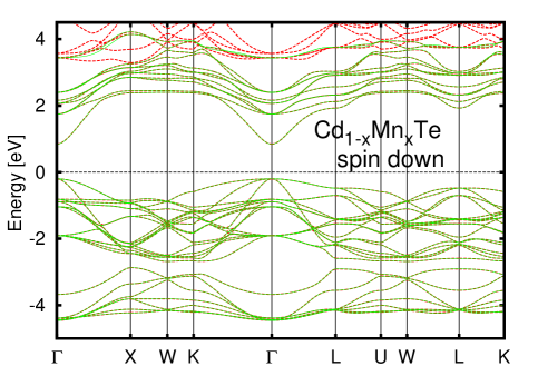
Figure 1: GGA band structure obtained using the MLWF for Cd_0.875Mn_0.125Te, $U_{\text{Mn}}=5$ eV, and assuming ferromagnetic alinement of Mn spins without spin-orbit coupling. A grey (red) dashed line in the left (right) panel depicts the spin up (down) channel. The interpolated Cd-$s$, Te-$p$, and Mn-$d$ Wannier bands are shown by a solid green line. Zero energy is set at the valence band top.

In our work, we focused on Mn content $x=2/64,4/64$, and $8/64$. Since we look for magnitudes of $sp$-$d$ exchange splittings, the Mn magnetic moments are always ferromagnetically aligned. The Hubbard $U$ effects for Mn open $d$ shell have been included. We use the values of $U_{\text{Mn}}=3$, 5 and 7 eV Paul et al. (2014); Autieri and Sanyal (2014); Keshavarz et al. (2017) and $J_{\text{H}}=0.15U$ eV for the Mn-$3d$ states. After obtaining the Bloch wave functions in density functional theory, the maximally localized Wannier functions Marzari and Vanderbilt (1997); Souza et al. (2001) (MLWF) are constructed using the WANNIER90 code Mostofi et al. (2008). We used the Slater-Koster interpolation scheme based on Wannier functions to extract electronic bands’ character at low energies.

Quantities of interest here are effective exchange energies $J_{c}({\bm{k}})$ and $J_{v}({\bm{k}})$ calculated from ${\bm{k}}$-dependent splittings of the lowest conduction and highest valence bands, generated by exchange interactions with Mn spins $S=5/2$, aligned by an external magnetic field,

$$J_{c}(\bm{k})=\frac{{\Delta}E_{c}}{xS}=\frac{E_{c}^{\downarrow}-E_{c}^{\uparrow}}{xS},\quad J_{v}(\bm{k})=\frac{{\Delta}E_{v}}{xS}=\frac{E_{v}^{\downarrow}-E_{v}^{\uparrow}}{xS}.$$ (1)

According to this definition, in the weak coupling limit and for the normal band ordering, i.e., for Cd_1-xMn_xTe, $J_{c}(k=0)\equiv N_{0}\alpha$ and $J_{v}(k=0)\equiv N_{0}\beta$, where $N_{0}$ is the cation concentration, whereas $\alpha$ and $\beta$ are $s$-$d$ and $p$-$d$ exchange integrals according to the DMS literature Kacman (2001); Wei and Zunger (1987); Larson et al. (1988). The same situation takes place in the case of Hg_1-xMn_xTe with $x\gtrsim 0.07$ Furdyna (1988). However, at lower $x$, Hg_1-xMn_xTe is a zero-gap semiconductor with an inverted band structure (topological zero-gap semiconductor) for which the $s$-type $\Gamma_{6}$ band is below the $\Gamma_{8}$ $j=3/2$ multiplet forming the conduction and valence bands. In this case, we consider the spin-splitting of the $\Gamma_{6}$ band below the Fermi level as $J_{c}$. We note also that because of antiferromagnetic interactions between Mn spins, an effective Mn concentration $x_{\text{eff}}$ that contributes to the $sp-d$ exchange splitting of bands in a magnetic field is much smaller than $x$, typically $x_{\text{eff}}\lesssim 5$% for any $x$ in relevant magnetic fields $\mu_{0}H\lesssim 6$ T Gaj et al. (1979). For random distribution of Mn over cation sites, these antiferromagnetic interactions result in spin-glass freezing at low temperatures Galazka et al. (1980); Mycielski et al. (1984).

III Results

III.1 GGA band structure for Cd_1-xMn_xTe and Hg_1-xMn_xTe without spin-orbit coupling

We discuss first the electronic structure of Cd_1-xMn_xTe and Hg_1-xMn_xTe computed with relativistic corrections in the scalar approximation, i.e., taking into account the Darwin and mass-velocity terms (essential in Hg_1-xMn_xTe) but neglecting SOC. Such an approach allows us to extract spin splittings solely due to the exchange interactions between host and Mn spins, i.e., effective exchange integrals $J_{c}$ and $J_{v}$ for relevant bands and arbitrary $\bm{k}$-vectors in the Brillouin zone.

Figure 1 presents the electronic structure of Cd_0.875Mn_0.125Te for spin up and spin down evaluated assuming $U_{\text{Mn}}=5$ eV. The Mn lower and upper Hubbard $3d$-bands reside around 4.6 eV below and 2.5 eV above the valence band top, respectively. Hence, in agreement with photoelectron spectroscopy Mizokawa et al. (2002), an effective Hubbard energy of Mn-$3d$ electrons is 7.1 eV for $U_{\text{Mn}}=5$ eV and, of course, would increase with the increasing $U_{\text{Mn}}$. At the same time, experimental data Mizokawa et al. (2002) indicate that the Mn $d$-bands reside by about 1 eV higher with respect to host bands than implied by our DFT results. In the whole Brillouin zone and for both spin channels, the lowest unoccupied states consist mainly of Cd-$5s$ states, whereas Te-$5p$ states give a dominant contribution to the highest occupied bands. To estimate the orbital contribution in DFT, we evaluate the system at the $\Gamma$ point, where the $s$-states are decoupled from the $p$ and $d$-states. For the (Mn,Cd)Te, the conduction band is composed roughly by 70% Cd-$s$ states and 30% Te-$s$ states with a minor contribution from the impurity Mn-$s$ states for the low Mn concentration $x$ in question. The conduction band at the $\Gamma$ point is composed roughly by 80% Te-$p$ states and 20% Cd-$d$ states with a minor contribution from the impurity Mn-d states.

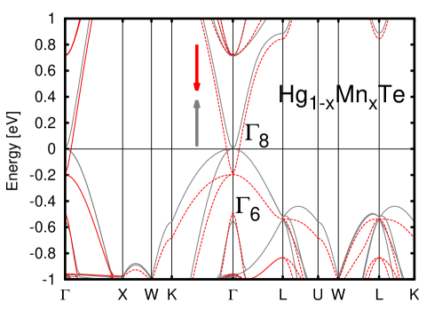
Figure 2: GGA band structure of Hg_0.875Mn_0.125Te with ferromagnetically aligned Mn spins without spin-orbit coupling and for $U_{\text{Mn}}=5$ eV. Zero energy is set at the valence band top. Bands for spin up and spin down with respect to Mn spins’ direction are shown by solid grey and red dash lines, respectively.

From the electronic structure of Hg_0.875Mn_0.125Te at $U_{\text{Mn}}=5$ eV without SOC, the effective Hubbard energy of Mn-$3d$ electrons at the $\Gamma$ point is 7.8 eV for $U_{\text{Mn}}=5$ eV. As shown in Fig. 2, the $\Gamma_{6}$ and $\Gamma_{8}$ bands are inverted in Hg_1-xMn_xTe, resulting in a topological character of the compound. The relativistic Darwin term gives a weak positive contribution to the energy of the $s$-bands in heavy atoms like Hg. In contrast, the relativistic mass-velocity term provides a strong negative energy shift, accounting for the band inversion. We can see in Fig. 2 that the $\Gamma_{6}$ band at 0.5 eV below the Fermi level, has the spin up component at lower energies indicating the ferromagnetic sign of the exchange interaction with Mn spins. Instead, the carrier spins in the $\Gamma_{8}$ bands are antiferromagnetically coupled to Mn spins.

III.2 Spin splitting along the k path without spin-orbit coupling

To take random Mn positions into account, we have used the SQS for determining the ${\bm{k}}$-dependence of exchange energies $J_{c}$ and $J_{v}$. Figure 3 shows $J_{c}(\bm{k})$ and $J_{v}(\bm{k})$ computed for Cd_1-xMn_xTe with various Mn concentrations $x$ and $U_{\text{Mn}}=5$ eV. In agreement with the experimental results Gaj et al. (1979), the values determined for the $\Gamma$ point do not depend on $x$, and their DFT values, $N_{0}\alpha=0.28$ eV and $N_{0}\beta=-0.63$ eV, describe the sign, and also reasonably well the experimental magnitudes, $N_{0}\alpha=0.22$ eV and $N_{0}\beta=-0.88$ eV Gaj et al. (1979), depicted by horizontal lines in Fig. 3. The exchange splittings at $\Gamma$ means that there is a large energy difference between transitions from the two heavy hole subbands (or for the creation of the heavy hole excitons). This giant Zeeman splitting is described by $\Delta E=xS(N_{0}\alpha-N_{0}\beta)$.

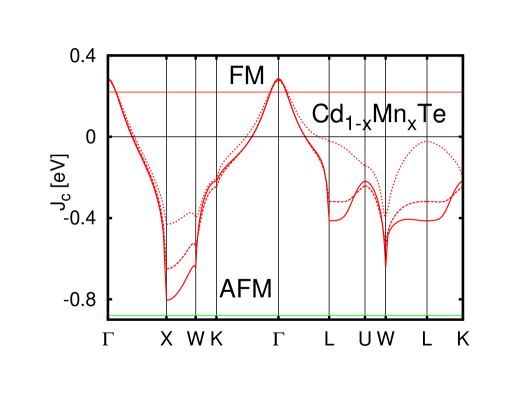
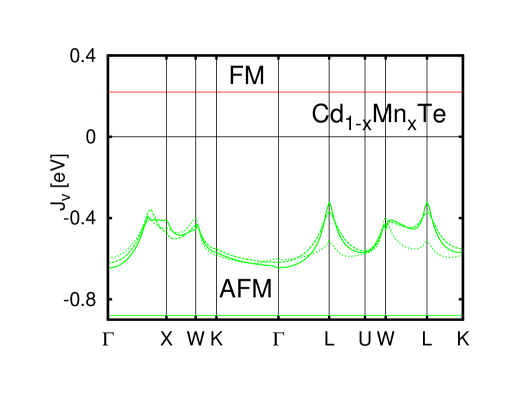
Figure 3: GGA values of effective exchange integrals for the conduction and valence band, $J_{c}$ in the top panel (red lines) and $J_{v}$ in the bottom panel (green lines) for Cd_1-xMn_xTe compared to experimental values at the $\Gamma$ point, determined by exciton magnetospectroscopy, represented by horizontal lines Gaj et al. (1979). The experimental effective exchange integral is positive for the conduction band and negative for the valence at the $\Gamma$ point. The solid, dashed, and dotted lines represent the band spin splitting for entirely spin-polarized Mn ions with concentrations $x=2/64=0.03125,4/64=0.0625$ and $8/64=0.125$, respectively. The computations have been performed neglecting spin-orbit coupling and for $U_{\text{Mn}}=5$ eV.

As seen, $J_{v}$ remains negative (antiferromagnetic) for all $\bm{k}$-values, and its magnitude slightly oscillates along the $\bm{k}$-path, it reaches a maximum at $\Gamma$ and a minimum at $L$ for small Mn concentrations, and between the $\Gamma$ and $X$ points at the highest studied $x=8/64=0.125$.

In contrast to $J_{v}$, $J_{c}$ changes sign and is highly oscillating along the $\bm{k}$-path: the sign of $J_{c}$ is positive (ferromagnetic potential $s$-$d$ exchange) at the $\Gamma$ point, in which the conduction band wave function has the $s$-type character, but becomes antiferromagnetic away from the $\Gamma$ point. This behavior originates from an admixture of anion wave functions to the Bloch amplitudes $u_{\bm{k}}$ and, thus, from a significant role of antiferromagnetic $sp$-$d$ kinetic exchange, affected by the phase factors $\exp(i\bm{k}\cdot\bm{r})$, known from the Kondo physics in dilute magnetic metals Schrieffer and Wolff (1966). In the negative sign region, the absolute value of $J_{c}$ reaches a maximum at the $X$ points and a minimum at the $U$ points at small concentrations and at the $L$ points for $x=0.125$. Such a dependence results from an increase of $sp$-$d$ hybridization and, thus, of the kinetic exchange if a given state approaches the $3d$ Mn shell, in the $J_{c}$ case, the upper Hubbard $3d^{6}$ band. In agreement with this interpretation, exchange energies at the boundary of the Brillouin zone get reduced when we increase $U_{\text{Mn}}$ because the Mn $d$-states move away from the relevant bands, and the hybridization between the host bands and the $3d$ shells of Mn-impurities becomes suppressed.

We are interested in the origin of a large reduction in magnitudes of exchange splittings at $L$ compared to $\Gamma$, as determined by interband magnetooptical studies. The corresponding reduction factor can then be defined as

$$r=\frac{J_{c}(\Gamma)-J_{v}(\Gamma)}{J_{c}(L)-J_{v}(L)}.$$ (2)

As seen, the sign of $r$ is determined by relative magnitudes of $J_{c}$ and J$v$, whose values and signs at the Brillouin zone boundary depend on a subtle competition between positive (ferromagnetic) potential and negative (antiferromagnetic) kinetic exchange energies. According to ab initio results presented in Fig. 3, $J_{c}$ and $J_{v}$ at the $L$ points have the same sign and similar magnitudes. This fact explains qualitatively why the experimentally observed splitting of optical spectra is relatively small at $L$ compared to $\Gamma$ Ginter et al. (1983); Coquillat et al. (1986); Ando et al. (2011). Given our results, the previous attempt to interpret the large value of $r$ was quantitatively unsuccessful because a strong dependence of $J_{c}$ on $\bm{k}$ was disregarded Bhattacharjee (1990). At the same time, our data suggest a relatively strong dependence of $J_{c}$ and $J_{v}$ at $L$ on $x$. Experimental results accumulated so far do not corroborate this expectation.

Finally, we mention the relevance of our ab initio results for magnetooptical studies of (001)Cd_1-xMn_xTe quantum wells sandwiched between Cd_1-x-yMn_xMg_yTe barriers Mackh et al. (1996); Merkulov et al. (1999), interpreted theoretically by a $k\cdot p$ model Merkulov et al. (1999). Experimental data pointed to a reduction of exchange splittings compared to those found for bulk samples, the behavior assigned to effectively non-zero values of $k\sim\pi/d$ ($d$ is the quantum well thickness) at which splittings were probed Mackh et al. (1996); Merkulov et al. (1999). Our evaluation, making use of data in Figs. 3 and 1 for the relevant ${\bm{k}}$-direction (the $\Gamma$-$X$ line) indicates that the decrease of $J_{c}$ with $\bm{k}$ is consistent with the experimentally observed and theoretically described decrease of $N_{0}\alpha$ with diminishing $d$, if penetration of the wave function into barriers is taken into account Merkulov et al. (1999).

Figure 4 shows $J_{c}(\bm{k})$ and $J_{v}(\bm{k})$ extracted from the band structure computations without SOC for Hg_1-xMn_xTe with different values of $x$. In the vicinity of the zone center we present single data points corresponding to the exchange energy of the $\Gamma_{6}$ band, i.e., $N_{0}\alpha$. The trends in $\bm{k}$ dependencies are similar to the Mn-doped CdTe. In particular, $J_{v}$ stays negative in the whole Brillouin zone and $J_{c}(\bm{k})$ becomes negative away from the zone center.

On the experimental side, there are two sets of the determined $N_{0}\alpha$ and $N_{0}\beta$ values, differing by more than a factor of two, in the case of Hg_1-xMn_xTe Dietl (1994). Our computational results point to the lower values, i.e., $N_{0}\alpha=0.4$ eV and $N_{0}\beta=-0.6$ eV Furdyna (1988); Dobrowolska and Dobrowolski (1981). Furthermore, according to experimental findings, magnetic circular dichroism at $L$ has the same sign for Hg_1-xMn_xTe as found for Cd_1-xMn_xTe at $L$ and at $\Gamma$, independently of Mn content $x$ Coquillat et al. (1989). Our data suggest the opposite sign since, according to the results in Fig. 4, $J_{c}(L)-J_{v}(L)<0$ for Hg_1-xMn_xTe in the relevant effective Mn concentrations, $x\lesssim 6$%.

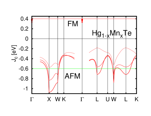
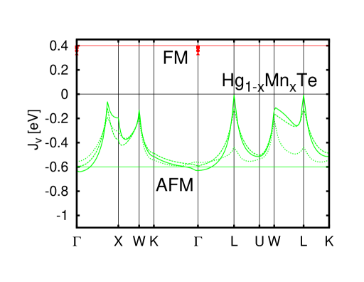
Figure 4: The values of effective exchange integrals for the conduction and valence band, $J_{c}$ in the top panel (red lines) and $J_{v}$ in the bottom panel (green lines) for Hg_1-xMn_xTe compared to experimental values at the $\Gamma$ point represented by horizontal lines Furdyna (1988); Dobrowolska and Dobrowolski (1981). The sign of the experimental effective exchange integral is negative for the valence band and positive for the conduction band at the $\Gamma$ point. The solid, dashed, and short-dashed represent the spin splitting for $x=2/64=0.03125,4/64=0.0625$ and $8/64=0.125$, respectively. The square, circle and triangle represent an effective exchange integral of the $\Gamma_{6}$ band for $x=2/64=0.03125,4/64=0.0625$, and $8/64=0.125$, respectively.

In summary, the DFT results presented in Figs. 3 and 4, obtained without taking SOC into account, have qualitatively shown how exchange spin-splitting of bands evolves with the ${\bm{k}}$-vector spanning the whole Brillouin zone. This dependence reflects (i) the $\bm{k}$-dependent mixing between cation and anion wave functions, which affects a relative contribution of the potential and kinetic components to the $sp$-$d$ exchange and (ii) the energy position of a given ${\bm{k}}$ state with respect to the open Mn $d$ shells, which controls the magnitude of the $\bm{k}$-dependent kinetic exchange. Quantitatively, however, bands’ energy position and, thus, the magnitude of exchange splitting depends significantly on SOC. Moreover, in the presence of SOC, exchange splitting of a given band state changes with the orientation of its ${\bm{k}}$-vector with respect to the direction of ${\bm{M}}(T,{\bm{H}})$. This means that, in general, exchange splitting of particular $L$ valleys differs, depending on the angle between ${\bm{k}}_{L}$ and ${\bm{M}}(T,{\bm{H}})$. Furthermore, under non-zero magnetization ${\bm{M}}(T,{\bm{H}})$, degeneracy of states with different projections of the orbital momentum is removed in the presence of SOC. This results in MCD, i.e., different transition probabilities for two circular light polarizations $\sigma^{+}$ and $\sigma^{-}$. In other words, MCD vanishes in the absence of SOC and, neglecting the magnetic field’s direct effect on electronic states, in the absence of exchange-induced spin splittings.

We are interested in interpreting MCD for Cd_1-xMn_xTe and Hg_1-xMn_xTe, taken at photon energies corresponding to free excitons at the fundamental gap at the $\Gamma$ point ($E_{0}$ and $E_{0}+\Delta_{0}$ transitions) and at the $L$ points ($E_{1}$ and $E_{1}+\Delta_{1}$ transitions) Ginter et al. (1983); Coquillat et al. (1986); Ando et al. (2011); Coquillat et al. (1989), where $\Delta_{0}$ and $\Delta_{1}$ are the spin-orbit splitting of the valence band at the $\Gamma$ and $L$ points of the Brillouin zone, respectively. Our theoretical approach considering SOC involves several steps. First, we use the DFT calculations with SOC taken into account to determine the parameters of a tight-binding model for CdTe and HgTe. Second, we consider the Mn-doped case and obtained from DFT on-site and hopping energies for Mn $d$ shell and its coupling to band states in CdTe and HgTe. Third, these parameters are incorporated into $sp$-$d$ exchange Hamiltonian that takes into account the presence of $\bm{k}$-dependent kinetic and potential exchange interactions in the molecular-field and virtual-crystal approximations suitable for Cd_1-xMn_xTe and Hg_1-xMn_xTe. In the fourth step, we use this model to determine energies of optical transitions at the $\Gamma$ and $L$ points of the Brillouin zone. We then develop the $\bm{k}\cdot\bm{p}$ theory for the $L$ point of the Brillouin zone in zinc-blende semiconductors, which allows as determining the oscillator strength for particular transitions and two circular light polarizations. With this information, we are in a position to compute the MCD spectra for Cd_1-xMn_xTe and Hg_1-xMn_xTe, and validate our approach by comparison to experimental data.

III.3 DFT with spin-orbit coupling and minimal tight-binding model for CdTe and HgTe

As mentioned in Sec. II, we use MBJLDA to determine the relativistic band structure of CdTe and HgTe with experimental lattice constants 6.48 Å for CdTe and 6.46 Å for HgTe. To extract energy dispersions $E(\bm{k})$ of the electronic bands, the Slater-Koster interpolation scheme is employed. The obtained results are shown in Fig. 5. The computed values of energy gaps and spin-orbit splittings for CdTe and HgTe are summarized in Table 1, and show good agreement with experimental data.

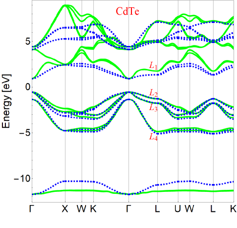
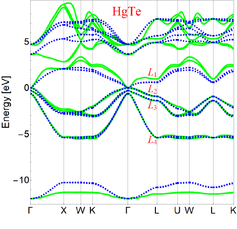
Figure 5: Comparison between the Wannier bands obtained by MBJLDA (solid green line) and our tight-binding model (dashed blue lines) for CdTe (left panel) and HgTe (right panel) taking spin-orbit coupling into account. The bands labeled $L_{1}$,$L_{2}$,$L_{3}$, and $L_{4}$ are described by irreducible representations of the double group $L_{6}$, $L_{4,5}$, $L_{6}$, and $L_{6}$, respectively.

We aim to use the ab initio results for determining the parameters of the one-electron Hamiltonian in the tight-binding approximation (TBA), which will adequately describe the band structure and $sp$-$d$ exchange splittings of bands at an arbitrary $\bm{k}$-point of the Brillouin zone with SOC taken into account. Similar to the previous descriptions of CdTe and HgTe within TBA Tarasenko et al. (2015), we consider $sp^{3}$ orbitals per atom and the nearest neighbor hopping. In particular, from positions of the electronic bands at $\Gamma$ we obtain the TBA on-site energies and the spin-orbit splittings. Then we use as constraints the DFT values of the band energies at the $\Gamma$, $X$, and $L$ points. We create an equation system and search for the values of the hopping energies $V$. If this procedure results in multiple solutions, we select $V_{sp}$ that has the same sign as the first-neighbor hopping energy among Wannier functions. The TBA parameters obtained in this way are shown in Table 2. Since the atomic radius of Cd is smaller than of Hg, whereas the bond length is greater in CdTe compared to HgTe, there are no systematic differences in the magnitudes of the hybridizations $V$ between these two compounds. Figure 5 presents a comparison of the band structures resulting from the MBJLDA and our TB model.

Table 1: Energy gaps and spin-orbit splittings (in eV) at the $\Gamma$ and $L$ points, where $E_{0}=E(\Gamma_{6})-E(\Gamma_{8})$ and $\Delta_{0}=E(\Gamma_{8})-E(\Gamma_{7})$ and at the $L$ points of the Brillouin zone, where $E_{1}=E(L_{1})-E(L_{2})$ and $\Delta_{1}=E(L_{2})-E(L_{3})$ for CdTe and HgTe, as determine from MBJLDA (our data), ETB Tarasenko et al. (2015), our TB model, and experimentally. Labeling of $L$ points is shown in Fig. 5.

CdTe
	MBJLDA	ETB	TB	expl
$E_{0}$	1.47	1.56	1.46	1.61 (Ref. Laurenti et al., 1990)
$\Delta_{0}$	0.81	0.78	0.80	0.95 (Ref. Twardowski et al., 1980)
$E_{1}$	3.03	4.78	2.63	3.28 (Ref. Cardona et al., 1967); 3.46 (Ref. Chadi et al., 1972)
$\Delta_{1}$	0.49	0.47	0.49	$0.6\pm 0.05$ (Ref. Cardona et al., 1967)

HgTe
	MBJLDA	ETB	TB	expl
$E_{0}$	-0.31	-0.22	-0.27	-0.30 (Ref. Laurenti et al., 1990)
$\Delta_{0}$	0.70	0.72	0.59	0.91 (Ref. Sakuma et al., 2011)
$E_{1}$	1.89	2.75	1.53	2.12 (Ref. Ando et al., 2011); 2.25 (Ref. Chadi et al., 1972)
$\Delta_{1}$	0.49	0.50	0.45	0.62–0.75 (Ref. Sakuma et al., 2011)

Table 2: Values of the on-site $E$, hopping $V$, and spin-orbit splitting $\Delta$ energies (in eV) of our minimal tight-binding model for CdTe and HgTe, which includes $sp^{3}$ orbitals of anions $a$ and cations $c$, and the nearest-neighbor hopping. Zero energy is set at the top of the valence band.

	CdTe	HgTe
$E_{s(a)}$	$-8.7752$	$-9.1555$
$E_{s(c)}$	$-0.9526$	$-3.1156$
$E_{p(a)}$	$-0.2669$	$-0.1742$
$E_{p(c)}$	$\hskip 8.5359pt4.8663$	$\hskip 8.5359pt4.3691$
$V_{ss}\sigma$	$-1.2431$	$-1.2569$
$V_{s(a)p(c)}\sigma$	$\hskip 8.5359pt1.6379$	$\hskip 8.5359pt1.7229$
$V_{s(c)p(a)}\sigma$	$\hskip 8.5359pt1.5463$	$\hskip 8.5359pt1.4834$
$V_{pp}\sigma$	$\hskip 8.5359pt2.0139$	$\hskip 8.5359pt2.2132$
$V_{pp}\pi$	$-0.9875$	$-0.9830$
$\Delta_{a}$	$\hskip 8.5359pt0.8025$	$\hskip 8.5359pt0.5915$
$\Delta_{c}$	$\hskip 8.5359pt0.2925$	$\hskip 8.5359pt1.0824$

By construction, the TB parameters collected in Table 2 lead to similar bandgaps and spin-orbit splittings as determine by DFT, and displayed in Table 1 and Fig. 5. These parameters describe well experimental energy gaps at both $\Gamma$ and $L$. For comparison, we present in Table 1 the magnitudes of bandgaps and spin-orbit splittings computed by using the tight-binding parameters determined by Tarasenko et al. Tarasenko et al. (2015) in reference to experimental data primarily at $\Gamma$.

III.4 Tight-binding parameters from DFT for Cd_1-xMn_xTe and Hg_1-xMn_xTe

We are interested in evaluating Slater-Koster parameters associated with the presence of open $3d$ shells of Mn in Cd_1-xMn_xTe and Hg_1-xMn_xTe, i.e., hopping energies between Mn $3d$ orbitals and $5sp^{3}$ states of the nearest neighbor Te anions as well as energetic positions of Mn $d$ levels. For this purpose, we use supercells with $2\times 2\times 2$ unit cells, each containing one Mn atom. The GGA+U technique is employed with $U_{\text{Mn}}=5$ eV and J${}_{\text{Hund}}=0.75$ eV as well as with the PBE exchange functional. Since in such alloys, no $E(\bm{k})$ dependencies can be derived, we extract the Slater-Koster parameters $V$ directly from the hopping energies among the relevant Wannier functions, which means that their accuracy is presumably of the order of 20%. The magnitudes of determined parameters are shown in Table 3. A lower position (by about 0.3 eV) of $d$ levels in HgTe compared to CdTe originates from the valence band offset between these two compounds Kowalczyk et al. (1986); Dietl and Kossut (1988). The spin-up Mn states are more localized and the hopping energies $V$ related to $d\uparrow$ are smaller. On the other hand, noticeable dissimilarities in hopping energies of the two compounds are caused by differences in the bond length and in the participation of cation orbitals to the $s$-like and $p$-like wave functions.

Table 3: The DFT values of on-site and hopping energies (in eV) for Mn $3d$ orbitals ($t_{2g}$ and $e_{g}$) and the nearest-neighbor Te $5s$ and $5p$ states for Cd_1-xMn_xTe and Hg_1-xMn_xTe. Zero energy is set at the top of the valence band.

	Cd1-xMnxTe	Hg1-xMnxTe
$E_{t2g\uparrow}$	$-4.702$	$-4.997$
$E_{t2g\downarrow}$	$\hskip 8.5359pt2.198$	$\hskip 8.5359pt1.821$
$E_{eg\uparrow}$	$-4.525$	$-4.858$
$E_{eg\downarrow}$	$\hskip 8.5359pt2.665$	$\hskip 8.5359pt2.293$
$V_{sd}\uparrow\sigma$	$-1.081$	$-1.232$
$V_{sd}\downarrow\sigma$	$-1.949$	$-1.957$
$V_{pd}\uparrow\sigma$	$-0.488$	$-0.364$
$V_{pd}\downarrow\sigma$	$-0.957$	$-0.987$
$V_{pd}\uparrow\pi$	$\hskip 8.5359pt0.253$	$\hskip 8.5359pt0.187$
$V_{pd}\downarrow\pi$	$\hskip 8.5359pt0.844$	$\hskip 8.5359pt0.854$

III.5 Tight-binding model with $sp$-$d$ exchange interaction

We now present and discuss the tight-binding Hamiltonian with four $sp^{3}$ orbital per atom containing a term describing giant Zeeman splitting of bands in the presence of spin polarized Mn ions. This splitting is brought about by: (i) the kinetic exchange resulting from spin-independent hybridization between Mn $3d$ shells and band states derived from the $5s$ and $5p$ orbitals of the four neighboring Te anions; (ii) direct (potential) exchange coupling of electrons residing on the open Mn $3d$ shell to band carriers visiting Mn $4s$ or $4p$ orbitals. Our approach is developed within the molecular-field and virtual-crystal approximations, and generalizes previous descriptions of DMSs within TBA Oszwałdowski et al. (2006); Sankowski et al. (2007) by taking into account the $\bm{k}$-dependence of the kinetic exchange according to,

$${\cal{H}}({\bm{k}})={\cal{H}}_{\text{TB}}({\bm{k}})+{\cal{H}}_{sp-d}({\bm{k}}).$$ (3)

Within our model ${\cal{H}}_{\text{TB}}(\bm{k})$ is a $16\times 16$ matrix, with on-site energies of $s$ and $p$ cation and anion orbitals on the diagonal; $\bm{k}$-dependent hopping $t_{mn}(\bm{k})$ between orbitals $m$ and $n$ of the nearest-neighbor (n.n.) cation-anion pairs, and the intraatomic spin-orbit term involving $p$-type orbitals of the cation and anion, respectively,

$$\left<m,s\middle|{\cal{H}}_{\text{TB}}(\bm{k})\middle|n,s^{\prime}\right>=E_{n}\delta_{mn}+t_{mn}(\bm{k})+\frac{\Delta_{a(c)}}{3}\sum_{\alpha}I^{\prime\alpha}_{mn}\sigma^{\alpha}_{ss^{\prime}},$$ (4)

where $t_{mn}(\bm{k})$ is the total hopping energy to the four n.n. atoms in the zinc-blende lattice including $\bm{k}$-dependent phase factors,

$$t_{mn}(\bm{k})=\sum_{\bm{R}_{m}\in\text{n.n.}(\bm{R}_{n})}V_{mn}(\bm{R}_{m}-\bm{R}_{n})\exp[i\bm{k}\cdot(\bm{R}_{m}-\bm{R}_{n})].$$ (5)

The Slater-Koster interatomic matrix elements (dependent on the direction cosines of the vector from the location $\bm{R}_{n}$ of the orbital $n$ to the location $\bm{R}_{m}$ of the orbital $m$) are denoted as $V_{mn}(\bm{R}_{m}-\bm{R}_{n})$, and their values for various combinations of orbitals ($ss\sigma$, $sp\sigma$, $pp\sigma$, $pp\pi$) are given in Table 2. The intraatomic spin-orbit splitting energies of the anion (cation) $p$ states are denoted by $\Delta_{a(c)}$, respectively, the orbital momentum operator $I^{\prime\alpha}_{\beta\gamma}$ in the Cartesian basis ($\alpha,\beta,\gamma=x,y,z$) can be written using the Levi-Civita symbol $\epsilon_{\alpha\beta\gamma}$ as $I^{\prime\alpha}_{\beta\gamma}=-i\epsilon_{\alpha\beta\gamma}$, and $(\sigma^{\alpha})_{\alpha=x,y,z}$ stand for the set of Pauli matrices.

The exchange interaction is taken into account in the molecular-field and virtual-crystal approximations: the weight, by which Mn spin polarization affects the band splittings, is described by the vector $\bm{X}=x_{\text{eff}}\bm{S}$, where $x_{\text{eff}}=x$ and $S=5/2$ if all Mn ions are spin polarized, and the direction of $\bm{S}$ is imposed by the external magnetic field. Hence, the vector $\bm{X}$ is related to Mn spin magnetization according to $\bm{M}=-g_{\text{Mn}}N_{0}\bm{X}$, where $g_{\text{Mn}}=2.0$ and $N_{0}$ is the cation concentration. Then, the relevant $sp$-$d$ exchange Hamiltonian, to be added to the TB Hamiltonian, assumes the form:

$$\left<m,s\middle|{\cal{H}}_{sp-d}(\bm{k})\middle|n,s^{\prime}\right>=-\frac{1}{2}\sum_{\alpha}X^{\alpha}\sigma^{\alpha}_{ss^{\prime}}\left[\frac{1}{S}\sum_{d}\left(\frac{1}{E_{d\uparrow}-E_{\bm{k}}}-\frac{1}{E_{d\downarrow}-E_{\bm{k}}}\right)t_{md}(\bm{k})t_{dn}(\bm{k})+\left<m\middle|J_{4s-3d}\hat{P}_{sc}+J_{4p-3d}\hat{P}_{pc}\middle|n\right>\right]$$ (6)

The first term in the brackets was given by Schrieffer and Wolff Schrieffer and Wolff (1966), and accounts for the kinetic exchange; this contribution is $\bm{k}$-dependent (via $E_{\bm{k}}$ and $t_{md}(\bm{k})t_{dn}(\bm{k})$), and may be non-diagonal. In this term, the $d$ index runs over the $t_{2g}$ and $e_{g}$ orbitals of Mn, the matrix of hoppings is defined as in Eg. (5), but this time takes into account the matrix of hoppings between cation $d$ orbitals and n.n. anion $s$ and $p$ orbitals, as given by Schrieffer and Wolff’s canonical transformation that is equivalent to the second order perturbation theory. Accordingly, as input parameters one should adopt the values unperturbed by the $sp$-$d$ hybridization. To this end, as $E_{d\uparrow,\downarrow}$ we take $E_{eg\uparrow,\downarrow}$, as $e_{g}$ states hybridize weakly in the tetrahedral case Wei and Zunger (1987), and as $V_{nd}$ spin average values of $V_{pd}\sigma$ and $V_{pd}\pi$ in Table 3. If relevant $d$ and ${\bm{k}}$ states cross, higher order perturbation theory is necessary Śliwa and Dietl (2018).

The second term in Eq. (6) describes intra-Mn direct (potential) exchange $J_{4s-3d}$ and $J_{4p-3d}$ between electrons residing on $3d$ and $4s$ or $4p$ Mn states, respectively; $\hat{P}_{sc}$ and $\hat{P}_{pc}$ are the projectors on cation $s$ and $p$ states. This ferromagnetic potential exchange assumes the canonical Heisenberg form, $-J\bm{s}\cdot\bm{S}$. According to spectroscopic studies, $J_{4s-3d}=0.392$ eV and $J_{4p-3d}=0.196$ eV for free Mn⁺¹ ions Dietl et al. (1994). The values of potential exchange are reduced in compound semiconductors by admixtures of anion orbitals to the Bloch wave functions taken into account within TBA and, possibly, also by screening (neglected here).

By incorporating Eq. (6) into the TB Hamiltonian we obtain ${\bm{k}}$-dependent splittings of bands for a given direction of Mn magnetization ${\bm{M}}$, from which the magnitudes of $sp$-$d$ exchange energies $J$, i.e., band splittings divided by $Sx_{\text{eff}}$ can be determined, as defined in Eq. (1). Table 4 shows the magnitudes of $J$ for conduction and valence bands at the $\Gamma$ and $L$ points of the Brillouin zone, relevant to interband magnetooptical transitions $E_{0}$, $E_{0}+\Delta_{0}$, $E_{1}$, and $E_{1}+\Delta_{1}$, respectively. These values have been obtained for $x_{\text{eff}}=0.0625$ and making use of the TB parameters determined from DFT and collected in Tables 2 and 3. Particular $J$ values have been determined by independent diagonalization of the TB Hamiltonian containing $E_{\bm{k}}$ in the kinetic exchange term (Eq. 6) corresponding to the band extremum in question, computed by diagonalizing the TB Hamiltonian without $sp$-$d$ exchange.

Table 4: Exchange energies $J(\bm{k})$ (in eV) for the conduction and valence bands at the $\Gamma$ and $L$ points of the Brillouin zone computed for Cd_1-xMn_xTe and Hg_1-xMn_xTe with $x_{\text{eff}}=0.0625$ employing tight-binding parameters displayed in Tables 2 and 3. In the DMS nomenclature, $J(\Gamma_{6})$ and $J(\Gamma_{8})$ correspond to $N_{0}\alpha$ and $N_{0}\beta$, respectively. Since for the $L_{2}$ and $L_{3}$ case the values of $J$ are anisotropic, we show in this Table the data are for the magnetization vector ${\bm{M}}\|[111]$ and for the $[111]$ $L$ valley. Labeling of $L$ bands is shown Fig. 5.

band	Cd1-xMnxTe		Hg1-xMnxTe
	TB	expl	TB	expl
$\Gamma_{6}$	$\hskip 8.5359pt0.32$	$\hskip 8.5359pt0.22$ (Ref. Gaj et al., 1979)	$\hskip 8.5359pt0.30$	$\hskip 8.5359pt0.40$ (Ref. Furdyna, 1988)
$\Gamma_{8}$	$-0.78$	$-0.88$ (Ref. Gaj et al., 1979)	$-0.74$	$-0.60$ (Ref. Furdyna, 1988)
$\Gamma_{7}$	$\hskip 8.5359pt0.24$	$\hskip 8.5359pt0.29$ (Ref. Twardowski et al., 1980)	$\hskip 8.5359pt0.22$
$L_{1}$	$-0.36$		$-0.22$
$L_{2}$	$-0.41$		$-0.35$
$L_{3}$	$-0.42$		$-0.33$

The theory reproduces the signs and magnitudes of exchange energies at $\Gamma$ properly. Furthermore, computed data point to a substantial difference in the exchange energy for the conduction band at $L$ compare to $\Gamma$, disregarded in previous theories of MCD at the $L$ point of the Brillouin zone in Cd_1-xMn_xTe Bhattacharjee (1990). A negative sign and a relatively large magnitude of this exchange energy obtained for Cd_1-xMn_xTe, $J_{c}(L_{1})=-0.36$, results from a substantial contribution of the antiferromagnetic kinetic exchange brought about by the proximity of the $L_{1}$ band to the Mn upper Hubbard band, the effect described by Eq. (6) and anticipated by ab initio results shown in Fig. 3. The role of kinetic exchange is smaller in Hg_1-xMn_xTe, where $J_{c}(L_{1})=-0.22$ eV, because the relativistic mass-velocity term, large at Hg atoms, shifts downward the conduction band in Hg_1-xMn_xTe. This shift makes that the $\Gamma_{6}$ band is below the $\Gamma_{8}$ band in Hg_1-xMn_xTe with low Mn content $x$, so that the material becomes a topological semimetal.

In the case of the $L_{2}$ and $L_{3}$ valence bands, SOC results in spin-momentum locking that diminishes spin-splitting in valleys oblique to the magnetization direction. According to Eqs. (114)-(116), the corresponding geometric factor is given by $\cos[\angle(\mathbf{k}_{L},\mathbf{M})]$ for the $L_{2}$ band; the formulas in the Appendix can be used for deriving geometry-dependent reduction factors for the two remaining valence bands. Thus, as noted previously Bhattacharjee (1990), a meaningful MCD theory for $E_{1}$ and $E_{1}+\Delta_{1}$ transitions requires the evaluation of exchange splittings and transition probabilities for each $L$ valley at a given magnetization direction.

The decomposition of the total Hamiltonian into the exchange-independent and exchange-dependent parts [Eq. (3)] as well as the use of the Schrieffer-Wolff transformation and atomic values of the potential exchange [Eq. (6)] allows one describing low-energy spin-related effects by a simple Kondo-like Hamiltonian. In order to check a quantitative accuracy of the Schrieffer-Wolff transformation, we have computed the p-d exchange energy N${}_{0}\beta$ by incorporating the Mn d-levels into the TB model employing values of d-level energies and hybridization matrix elements (weighted by x${}_{eff}^{1/2}$) collected in Table III. For x_eff = 0.0625, we obtain N${}_{0}\beta$ = -0.76 and -0.72 eV for Cd_1-xMn_xTe and Hg_1-xMn_xTe, respectively, the values within 3% in agreement with the theoretical data displayed in Table IV, $N_{0}\beta=-0.78$ and $-0.74$ eV, respectively.

III.6 Magnetic circular dichroism for $E_{1}$ and $E_{1}+\Delta_{1}$ transitions

In order to interpret quantitatively experimental studies of MCD at helium temperatures Ginter et al. (1983); Coquillat et al. (1986); Ando et al. (2011); Coquillat et al. (1989), we have to determine energies and oscillator strengths for optical transitions at the $L$ points of the Brillouin zone. The experimental data were collected in the Faraday configuration for $\sigma^{+}$ (electron cyclotron resonance active) and $\sigma^{-}$ light polarizations, and provided $\Delta E$, that is the difference in spectral positions of edges observed at these two polarizations. This optical exchange splitting $\Delta E$ was found to scale with magnetization, and was independently determined for spectral regions corresponding to $E_{1}$ and $E_{1}+\Delta_{1}$ transitions. In the presence of non-zero magnetization, the four $L$ valleys may not be equivalent and, thus, show different exchange splittings in the presence of SOC. Accordingly, in general, we expect that spectral features may consist of up to 16 excitonic lines in the vicinity of both $E_{1}$ and $E_{1}+\Delta_{1}$ energy gaps, corresponding to optical transitions $L_{2}\rightarrow L_{1}$ and $L_{3}\rightarrow L_{1}$, respectively. According to the bands’ dispersion at the $L$ point shown in Fig. 5, and similarly to the case of other zinc-blende semiconductors Tanimura and Tanimura (2020), $E_{1}$ and $E_{1}+\Delta_{1}$ optical transitions have a character of saddle-point excitons at low temperatures.

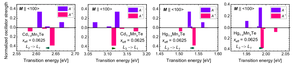
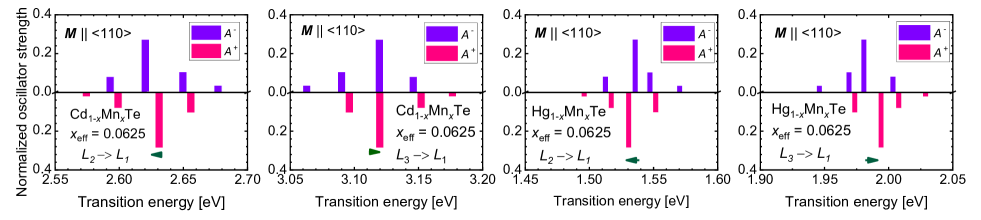
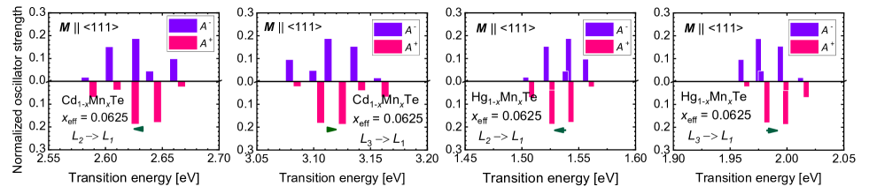
Figure 6: Normalized absorption ${\cal A}_{\iota\varphi}^{\pm}$ for $\sigma^{+}$ and $\sigma^{-}$ polarizations (positive and negative bars, respectively) for optical transitions in the vicinity of the $E_{1}$ and $E_{1}+\Delta_{1}$ gaps at $L$ points in the Brillouin zone for Cd_1-xMn_xTe (left panels) and Hg_1-xMn_xTe (right panels) with $x_{\text{eff}}=0.0625$ and fully polarized Mn spins along $\langle 100\rangle$, $\langle 110\rangle$, or $\langle 111\rangle$ crystal axis that is also the light propagation direction (upper, middle, and bottom panels, respectively). Arrows show the resulting spectral splittings at $L$, $\Delta E$, defined as a distance between the centers of gravity of lines appearing for $\sigma^{-}$ and $\sigma^{+}$ polarizations, respectively. In the case of Cd_1-xMn_xTe, $\Delta E$ at $E_{1}$ is about 30 times smaller than at $E_{0}$ for the same Mn magnetization. Note that MCD is usually defined as the difference ${\cal A}^{-}-{\cal A}^{+}$.

Our tight-binding Hamiltonian (Eq. 3) allows us to obtain directly expected optical transition energies $E_{\iota\varphi}=E_{\varphi}-E_{\iota}$ between states $\iota$ (initial) and $\varphi$ (final) at critical points of the valence and conduction subbands in a particular $L$-valley at ${\bm{k}}_{L}$ and at a given magnetization $\bm{M}$. We assume the transition probabilities at photon energies $h\nu=E_{\iota\varphi}$ are proportional, in the dipole approximation, to the square of the interband momentum matrix elements, i.e., we have for the oscillator strength $f_{\iota\varphi}^{\pm}$,

$$f_{\iota\varphi}^{\pm}=\frac{2|\langle\iota|p^{\pm}|\varphi\rangle|^{2}}{m_{0}(E_{\varphi}-E_{\iota})},$$ (7)

where $p^{\pm}=(p_{x}\pm\mbox{i}p_{y})/\sqrt{2}$ for $\sigma^{\pm}$ polarization, respectively, in a right-handed coordinate system $(x,y,z)$ with $z$ being here the optical axis, and $m_{0}$ is the free electron mass.

The determination of dipole matrix elements is somewhat ambiguous within TBA Leung and Whaley (1997); Lee et al. (2018). Similarly, the use of the Peierls-substitution for the determination of the momentum matrix elements in the presence of the vector potential Graf and Vogl (1995) triggered an extensive debate about the correctness Pedersen et al. (2001); Sandu (2005) and gauge invariance of such a procedure Boykin et al. (2001); Foreman (2002). Accordingly, optical spectra have been often evaluated within a poorly justified constant momentum matrix element approximation Czyżyk and Podgórny (1980) or by treating the momentum matrix elements as a fitting parameter Leung and Whaley (1997). As shown in Appendix, we have derived, employing a method of invariants, a $\bm{k}\cdot\bm{p}$ Hamiltonian for the $L$ valleys in zinc-blende semiconductors [equation (93)]. A similar formalism was elaborated earlier for the $L$-valleys in Ge and other semiconductors crystallizing in the diamond structure Li et al. (2012). Our general approach, for the $L$ points in zinc-blende semiconductors, takes the inversion asymmetry into account, which results in the presence of terms linear in the ${\bm{k}}$-vector, absent in the diamond structure. Inherently to this approach, both $f_{\iota\varphi}^{\pm}$ and the effective masses depend on the interband matrix elements $\bm{p}_{vc}$, described by two real material parameters $A$ and $B$. In particular, the inverse effective masses (longitudinal $1/m_{l}$ and transverse $1/m_{t}$), characterizing constant energy ellipsoids in the bands denoted as $L_{1}$ ($L_{6}$ representation) and $L_{2}$ ($L_{4,5}$ representation), have contributions proportional to $A^{2}$ (longitudinal one) and $B^{2}$ (the transverse one). This is consistent with $|A|\ll|B|$, as $m_{l}\gg m_{t}$ according to ab initio results showed in Fig. 5. Moreover, the magnitudes of $f_{\iota\varphi}$ (for the $E_{1}$ and $E_{1}+\Delta_{1}$ features) depend mostly on the value of $B$. These imply that the normalized absorbances ${\cal A}_{\iota\varphi}^{\pm}$, i.e., $f_{\iota\varphi}^{\pm}$ divided by the sum of all $f_{\iota\varphi}^{\pm}$ for either $E_{1}$ or $E_{1}+\Delta_{1}$ transitions, are immune (within 1%) to the numerical values of $A$ and $B$ as long as $|A|\lesssim|B|$. Accordingly, theoretical values of MCD can be obtained with no adjustable parameters.

Figure 6 shows computed ${\cal A}_{\iota\varphi}^{\pm}$ values for $E_{1}$ and $E_{1}+\Delta_{1}$ transitions involving all four $L$ valleys in Cd_1-xMn_xTe and Hg_1-xMn_xTe in the presence of magnetization $\bm{M}$, produced by spin-polarized Mn ions with the concentration $x_{\text{eff}}=0.0625$ and $S=5/2$, parallel to along either $\langle 100\rangle$, $\langle 110\rangle$, or $\langle 111\rangle$ crystalline axis, which is also the light propagation direction. The TBA has served to determine parameters for the $k\cdot p$ model (including exchange energies), which in turn has been used to obtain $E_{\iota\varphi}^{\pm}$ and ${\cal A}_{\iota\varphi}^{\pm}$.

In the case of ${\bm{M}}\|\langle 100\rangle$, there are four equivalent valleys tilted by $56.34^{\circ}$ to the light propagation direction, so that we expect that up to four optical transitions in both $E_{1}$ and $E_{1}+\Delta_{1}$ spectral ranges. Since the cleavage plane is $(110)$ for the zinc-blende structure, in the case of bulk single crystal samples Ginter et al. (1983); Coquillat et al. (1986, 1989), the magnetic field is presumably applied along the $\langle 110\rangle$ crystal axis. In this configuration, the ${\bm{k}}_{L}$ vector of two valleys is perpendicular, and of two others tilted by $35.25^{\circ}$ to the light direction. MCD studies were also carried out on thin films of Cd_1-xMn_xTe and Zn_1-xMn_xTe grown by molecular beam epitaxy on sapphire (0001) substrates, which resulted in (111) oriented polycrystalline samples Ando et al. (2011). In such a case, light propagates parallel to $L$ valley’s longitudinal axis, whereas ${\bm{K}}_{L}$ of three other valleys, if effects of strain and piezoelectric fields can be neglected, are tilted by $70.53^{\circ}$ to the light direction.

As seen in Fig. 6, there are four lines in each polarization for $\bm{M}\|\langle 100\rangle$ and $\bm{M}\|\langle 110\rangle$. Inspection of the $\bm{M}\|\langle 110\rangle$ data shows that the strongest and the weakest feature originate from the two oblique valleys, whereas the two other peaks from the valleys with ${\bm{k}}_{L}$ perpendicular to the magnetization and light direction, for which spin-momentum locking by SOC results in vanishing exchange splitting of the valence band states. In the case of $\bm{M}\|\langle 111\rangle$, the strongest line comes from the longitudinal valley, ${\bm{k}}_{L}\|\langle 111\rangle$; the four other lines originate from the three remaining oblique valleys. For comparison, at $E_{0}$ in Cd_1-xMn_xTe, two lines corresponding to the heavy and light excitons are resolved for each polarization. The heavy hole lines are three times stronger, and the energy difference between their positions in the two polarizations is taken as the magnitude of optical splitting $\Delta E$ at $\Gamma$, $\Delta E(E_{0})=x_{\text{eff}}S(N_{0}\alpha-N_{0}\beta)$. This procedure, taking $x_{\text{eff}}=0.0625$ and the theoretical values of the exchange energies shown in Table 4, leads to $\Delta E(E_{0})=0.17$ and $0.16$ eV for Cd_1-xMn_xTe and Hg_1-xMn_xTe, respectively. According to Fig. 6, the distances between the strongest lines at $L$ are much smaller, particularly in the case of Cd_1-xMn_xTe, implying $r=\Delta E(E_{0})/\Delta E(E_{1})=38$ and $-17$ for Cd_1-xMn_xTe and Hg_1-xMn_xTe, respectively, and ${\bm{M}}\|[110]$. Actually, taking into account intrinsically large broadening of excitonic transitions at $L$ (Ref. Tanimura and Tanimura (2020)), a better measure of spectral splitting provided by MCD is the distance between centers of gravity of lines appearing in $\sigma^{+}$ and $\sigma^{-}$ polarizations, as depicted by arrows in Fig. 6. In this case, $r=33$ and $13$ for the two compounds in question independently of magnetization orientations, the values in a qualitative agreement with the corresponding experimental data $r=16$ (ref. Coquillat et al. (1986); Ando et al. (2011)) and $5\pm 1$ (ref. Coquillat et al. (1989)), respectively. Our theory explains, therefore, a large difference between exchange splittings of optical spectra at $\Gamma$ and $L$ in bulk Ginter et al. (1983); Coquillat et al. (1986, 1989) and epitaxial Ando et al. (2011) Cd_1-xMn_xTe, hitherto regarded as highly surprising and contradicting theoretical expectations Ginter et al. (1983); Coquillat et al. (1986); Ando et al. (2011); Bhattacharjee (1990); Coquillat et al. (1989). The developed theory describes also the chemical trend, i.e., a significantly smaller magnitude of $r$ in topological Hg_1-xMn_xTe Coquillat et al. (1989) compared to topologically trivial Cd_1-xMn_xTe Ginter et al. (1983); Coquillat et al. (1986); Ando et al. (2011). On the other extreme, in the case of light Zn cations, greater value $r$ was found for bulk Zn_1-xMn_xTe or even sign reversal of $r$ in the case of epitaxial (111)Zn_1-xMn_xTe Ando et al. (2011). Furthermore, the computed values of $\Delta E(E_{1}+\Delta_{1})$ are seen in Fig. 6 to have the same amplitude but the opposite sign compared to $\Delta E(E_{1})$, as anticipated earlier Ginter et al. (1983); Bhattacharjee (1990) and observed experimentally for Hg_1-xMn_xTe Coquillat et al. (1989). Interestingly, no such reversal was fond in the case of epitaxial (111)Cd_1-xMn_xTe though it appears in epitaxial (111)Zn_1-xMn_xTe Ando et al. (2011).

IV Conclusions

By combining density functional theory with the modified Becke-Johnson exchange-correlation potential, a minimal tight-binding model, and envelope function formalisms at band extrema, we have accurately described experimental energy gaps and exchange splittings of magnetooptical spectra at the $\Gamma$ and $L$ points of the Brillouin zone in Mn-doped topologically trivial CdTe and topologically non-trivial HgTe with no adjustable or empirical parameters. In particular, according to our insight, a substantial reduction of the exchange-driven splittings at the $L$ points compared to the $\Gamma$ point, since long regarded as challenging Ginter et al. (1983); Coquillat et al. (1986); Ando et al. (2011); Bhattacharjee (1990); Coquillat et al. (1989), originates from the same sign and similar magnitudes of the exchange energies in the conduction and valence bands at $L$. More specifically, the negative exchange energy of the conduction band at $L$ results from (i) $\bm{k}$-dependent hybridization between band states and Mn open $d$ shells, which leads to the appearance antiferromagnetic kinetic exchange; (ii) $\bm{k}$-dependent changes in the orbital components of the Bloch functions, which affects the relative magnitudes of antiferromagnetic kinetic exchange and ferromagnetic potential exchange, and (iii) the proximity of the conduction band at $L$ to the upper Mn Hubbard band, which enlarges the role of kinetic exchange. This enlargement is more significant in Cd_1-xMn_xTe compared to Hg_1-xMn_xTe in which the relativistic mass-velocity term shifts downward $s$-orbitals of Hg contributing to the conduction band energy at $L$. The theory of magnetooptical phenomena also illustrates the interplay of exchange interactions with spin-orbit effects such as spin-momentum locking that diminishes exchange splitting of valence states in $L$-valleys that are oblique to the magnetization direction.

Supplementing previous tight-binding Hamiltonian designed for describing low-energy physics in topological HgTe-CdTe systems Tarasenko et al. (2015), our work provides tight-binding parameters appropriate to investigate phenomena dependent on global properties of the band structure, such as indirect exchange coupling between magnetic ions in magnetic semiconductors. At the same time, the derived $k\cdot p$ Hamiltonian is suitable for modeling phenomena involving $L$ valleys in all compounds with a zinc-blende crystal structure.

Appendix A Determination of the $k\cdot p$ Hamiltonian for the $L$-points in zinc-blende crystals

A.1 Construction of the representation for the zinc-blende valence band

Let $R_{0}$ be a lattice node (a cation or an anion site) of the zinc-blende lattice and let $G=T_{d}$ be the corresponding point group, generated by the operations $\{g_{a},g_{b}\}\subset G$ given in the Cartesian basis as:

$$g_{a}=\left(\begin{array}[]{ccc}0&1&0\\ -1&0&0\\ 0&0&-1\end{array}\right),\quad g_{b}=\left(\begin{array}[]{ccc}0&0&1\\ 1&0&0\\ 0&1&0\end{array}\right).$$ (8)

A representation $\Delta$ of the space group for the zinc-blende valence band is constructed following Ref. Bradley and Cracknell, 1972: let $k_{L}=\frac{\pi}{a_{0}}(1,1,1)$ be the $L$-symmetry point of the Brillouin zone, where $a_{0}$ is the lattice parameter. The corresponding Hilbert space $H_{k_{L}}$ of the Bloch states is spanned by the wave-functions $\{\psi_{X},\psi_{Y},\psi_{Z}\}\subset H_{k_{L}}$, denoted further as kets $X$, $Y$, and $Z$. The Hilbert space $H_{k_{L}}$ is the space of the representation $D:G\to B(H_{k_{L}})$ such that $g_{a}$ and $g_{b}$ are represented by the same matrices (8) in the basis $(X,Y,Z)$. The primitive translations $t\in\frac{a_{0}}{2}\{(0,1,1),(1,0,1),(1,1,0)\}$ act as

$$\Delta(t)\psi=\exp(-ik_{L}\cdot t)\psi,\qquad\psi\in H_{k_{L}}.$$ (9)

Thus the action of the subgroup

$$G_{k_{L}}=\{g\in G:gk_{L}\equiv k_{L}\}$$ (10)

coincides with the restriction of $D$, $\left.\Delta\right|_{G_{k_{L}}}=\left.D\right|_{G_{k_{L}}}$, while any other operation $g$ moves to another (non-equivalent) $L$-point of the Brillouin zone: $H_{k_{L}}\ni\psi\mapsto\Delta_{g}\psi\in H_{gk_{L}}$. There are four non-equivalent $L$-points in total,

$$Gk_{L}={}$$ (11)

$$\quad\frac{\pi}{a_{0}}\Bigl{\{}(1,1,1),(1,-1,-1),(-1,1,-1),$$

$$\quad\qquad(-1,-1,1)\Bigr{\}},$$

and the action of $D$ in this set defines the permutation matrices $r_{a}$ and $r_{b}$,

$$r_{a}=\left(\begin{array}[]{cccc}0&0&1&0\\ 1&0&0&0\\ 0&0&0&1\\ 0&1&0&0\end{array}\right),\qquad r_{b}=\left(\begin{array}[]{cccc}1&0&0&0\\ 0&0&0&1\\ 0&1&0&0\\ 0&0&1&0\end{array}\right).$$ (12)

Therefore,

$$\Delta(g_{a})=r_{a}\otimes g_{a},\qquad\Delta(g_{b})=r_{b}\otimes g_{b}.$$ (13)

This defines a representation of the space group.

A.2 Observables

Accordingly, any observable $\mathcal{O}$ is represented by a $12\times 12$ matrix, or a $4\times 4$ block matrix (with $3\times 3$ blocks). The action of the primitive translations separates the blocks of $\mathcal{O}$ in the sense that translation-invariant observables are block-diagonal. Moreover, the requirement of invariance with respect to point operations implies that any such observable is defined by the first block — the one corresponding to $H_{k_{L}}$. For example, scalar observables have the form

$$\mathcal{O}=\left(\begin{array}[]{ccc}a_{\mathcal{O}}&b_{\mathcal{O}}&b_{\mathcal{O}}\\ b_{\mathcal{O}}&a_{\mathcal{O}}&b_{\mathcal{O}}\\ b_{\mathcal{O}}&b_{\mathcal{O}}&a_{\mathcal{O}}\end{array}\right),$$ (14)

with two real-valued parameters, $(a_{\mathcal{O}},b_{\mathcal{O}})$.

Vector observables are defined by their Cartesian components, $(\mathcal{V}_{x},\mathcal{V}_{y},\mathcal{V}_{z})$:

$$\mathcal{V}_{x} = \left(\begin{array}[]{ccc}a_{\mathcal{V}}&b_{\mathcal{V}}&b_{\mathcal{V}}\\ c_{\mathcal{V}}&d_{\mathcal{V}}&e_{\mathcal{V}}\\ c_{\mathcal{V}}&e_{\mathcal{V}}&d_{\mathcal{V}}\end{array}\right),$$ (18)

$$\mathcal{V}_{y} = \left(\begin{array}[]{ccc}d_{\mathcal{V}}&c_{\mathcal{V}}&e_{\mathcal{V}}\\ b_{\mathcal{V}}&a_{\mathcal{V}}&b_{\mathcal{V}}\\ e_{\mathcal{V}}&c_{\mathcal{V}}&d_{\mathcal{V}}\end{array}\right),$$ (22)

$$\mathcal{V}_{z} = \left(\begin{array}[]{ccc}d_{\mathcal{V}}&e_{\mathcal{V}}&c_{\mathcal{V}}\\ e_{\mathcal{V}}&d_{\mathcal{V}}&c_{\mathcal{V}}\\ b_{\mathcal{V}}&b_{\mathcal{V}}&a_{\mathcal{V}}\end{array}\right).$$ (26)

A.3 Time-inversion symmetry

We assume for simplicity that the antiunitary time inversion operator $\hat{\mathcal{T}}$ acts independently on the orbital and spin degrees of freedom, i.e. it is a tensor product

$$\hat{\mathcal{T}}=\hat{K}\otimes\hat{T}_{1/2},\qquad$$ (27)

of some spin-independent part (denoted $\hat{K}$) and the usual time inversion for spin-$1/2$ particles:

$$\hat{T}_{1/2}:\psi=\left(\begin{array}[]{c}\psi_{\uparrow}\\ \psi_{\downarrow}\end{array}\right)\mapsto-i\sigma_{y}\overline{\psi}=\left(\begin{array}[]{c}-\overline{\psi_{\downarrow}}\\ \overline{\psi_{\uparrow}}\end{array}\right)$$ (28)

(the arbitrary phase factor being included in $\hat{K}$). Therefore, still disregarding the spin for now, we consider an anti-unitary involution $\hat{K}$,

$$\hat{K}\left(c\psi\right)=\overline{c}\hat{K}\psi,\qquad{\hat{K}}^{2}\psi=\hat{K}(\hat{K}\psi)=\psi$$ (29)

(cf. the relation $\hat{\mathcal{T}}^{2}=-1$ for fermions). It is defined by the matrix $K_{\alpha\beta}=\left<\psi_{\alpha}\middle|\hat{K}\psi_{\beta}\right>$, ($\alpha,\beta=X,Y,Z$), such that

$$\hat{K}\left(\sum_{\alpha}c_{\alpha}\psi_{\alpha}\right)=\sum_{\alpha,\beta}K_{\alpha\beta}\overline{c_{\beta}}\psi_{\alpha}.$$ (30)

Assuming that the representation of the extended symmetry group (space operations and time inversion) is a regular rather than a projective one,

$$\left(K_{\alpha\beta}\right)_{\alpha,\beta=X,Y,Z}=\left(\begin{array}[]{ccc}a_{T}&b_{T}&b_{T}\\ b_{T}&a_{T}&b_{T}\\ b_{T}&b_{T}&a_{T}\end{array}\right).$$ (31)

The pairs $(a_{T},b_{T})$ such that ${\hat{K}}^{2}=1$ can be further parameterized by $(u,v)$, $\left|u\right|=\left|v\right|=1$,

$$a_{T}=u\frac{v+2}{3},\qquad b_{T}=u\frac{v-1}{3},$$ (32)

and the matrix $\left(K_{\alpha\beta}\right)_{\alpha,\beta=X,Y,Z}$ assumes the form

$$K_{\alpha\beta}=u\left(\delta_{\alpha\beta}+\frac{v-1}{3}\right).$$ (33)

Since $u$ can be adjusted by changing the overall phase of the valence-band wave functions, one lets $u=1$.

A.4 Invariant Hamiltonian and the momentum operator

Accordingly, the invariant Hamiltonian for the valence band at the exact $L$-point reads

$$H_{inv}=\left(\begin{array}[]{ccc}a_{H}&b_{H}&b_{H}\\ b_{H}&a_{H}&b_{H}\\ b_{H}&b_{H}&a_{H}\end{array}\right).$$ (34)

The construction of a $k\cdot p$ Hamiltonian involves the momentum operator $\hat{p}$, which we discuss it in detail here. Momentum is represented as a time-inversion odd, vector operator. The operator equation $\hat{K}\hat{p}+\hat{p}\hat{K}=0$ defines a set of homogenous linear equations for the parameters $(a_{p},b_{p},c_{p},d_{p},e_{p})$ and their complex conjugates, see Eq. (A.8)-(26). In order to find the invariants one performs an $LDU$ decomposition of the coefficients’ matrix and investigates the zero entries on the diagonal of $D$. Special combinations of $(a_{T},b_{T})$ (or $u$ and $v$) are when a particular entry becomes zero. Therefore, two cases should be considered:

1. If $v=1$,

   $$\left(K_{\alpha\beta}\right)_{\alpha,\beta=x,y,z}=\left(\begin{array}[]{ccc}1&0&0\\ 0&1&0\\ 0&0&1\end{array}\right).$$ (35)

   and ($P$ real)

   $$\hat{p}_{x} = \frac{m_{0}P}{\hbar}\left(\begin{array}[]{ccc}0&i&i\\ -i&0&0\\ -i&0&0\end{array}\right),$$ (39)

   $$\hat{p}_{y} = \frac{m_{0}P}{\hbar}\left(\begin{array}[]{ccc}0&-i&0\\ i&0&i\\ 0&-i&0\end{array}\right),$$ (43)

   $$\hat{p}_{z} = \frac{m_{0}P}{\hbar}\left(\begin{array}[]{ccc}0&0&-i\\ 0&0&-i\\ i&i&0\end{array}\right).$$ (47)

2. If $v=e^{i\phi}\neq 1$,

   $$\left(K_{\alpha\beta}\right)_{\alpha,\beta=x,y,z}=\frac{1}{3}\left(\begin{array}[]{ccc}v+2&v-1&v-1\\ v-1&v+2&v-1\\ v-1&v-1&v+2\end{array}\right),$$ (48)

   and ($P$ real)

   $$\hat{p}_{x} = \frac{2}{3}\sin\left(\frac{\phi}{2}\right)\frac{m_{0}P}{\hbar}\left(\begin{array}[]{ccc}2&\frac{2+v}{1-v}&\frac{2+v}{1-v}\\ -\frac{1+2v}{1-v}&-1&-1\\ -\frac{1+2v}{1-v}&-1&-1\end{array}\right),$$ (52)

   $$\hat{p}_{y} = \frac{2}{3}\sin\left(\frac{\phi}{2}\right)\frac{m_{0}P}{\hbar}\left(\begin{array}[]{ccc}-1&-\frac{1+2v}{1-v}&-1\\ \frac{2+v}{1-v}&2&\frac{2+v}{1-v}\\ -1&-\frac{1+2v}{1-v}&-1\end{array}\right),$$ (56)

   $$\hat{p}_{z} = \frac{2}{3}\sin\left(\frac{\phi}{2}\right)\frac{m_{0}P}{\hbar}\left(\begin{array}[]{ccc}-1&-1&-\frac{1+2v}{1-v}\\ -1&-1&-\frac{1+2v}{1-v}\\ \frac{2+v}{1-v}&\frac{2+v}{1-v}&2\end{array}\right).$$ (60)

A.5 The $k\cdot p$ Hamiltonian

The standard derivation of $k\cdot p$ Hamiltonians involves perturbation theory and an expansion in the basis of the high-symmetry-point Bloch functions. Since in a typical semiconductor the result is dominated by terms due to virtual transitions to the conduction band, rather then giving the general form of the $k\cdot p$ Hamiltonian, here we write out an $8\times 8$ matrix (including the conduction band explicitly rather than via perturbation theory, and a spin-orbit term) which preserves the most important features of such systems. In the basis of $(S,X,Y,Z)$ states our Hamiltonian ${\cal H}$ reads:

$${\cal H} = \left(\begin{array}[]{cc}E_{c}+\frac{\hbar}{m_{0}}\mathbf{k}\cdot\hat{\mathbf{p}}_{c}&\frac{\hbar}{m_{0}}\mathbf{k}\cdot\hat{\mathbf{p}}_{vc}\\ \frac{\hbar}{m_{0}}\mathbf{k}\cdot\hat{\mathbf{p}}_{vc}^{\dagger}&H_{inv}+\frac{\hbar}{m_{0}}\mathbf{k}\cdot\hat{\mathbf{p}}\end{array}\right)$$ (64)

$$\qquad{}+\frac{1}{3}\lambda_{SO}(I^{\prime}_{x}\sigma_{x}+I^{\prime}_{y}\sigma_{y}+I^{\prime}_{z}\sigma_{z}),$$

where $\hat{\mathbf{p}}_{c}$ is the momentum operator in the conduction band (it is given in the next subsection in coordinates appropriate for the $L$-point). The valence band orbital momentum matrices $I^{\prime}_{\alpha}$ are defined as usual by the Levi-Civita symbol $(I_{\alpha})_{\beta\gamma}=-i\varepsilon_{\alpha\beta\gamma}$, $\alpha,\beta,\gamma=x,y,z$ by padding with zeros to a $4\times 4$ matrix, whereas $\sigma_{\alpha}$ are the Pauli matrices corresponding to the spin degree of freedom.

The interband matrices of momentum have the general form ($a_{pvc},b_{pvc}$ complex):

$$p_{vc,x} = \left(\begin{array}[]{ccc}a_{pvc}&b_{pvc}&b_{pvc}\end{array}\right),$$ (66)

$$p_{vc,y} = \left(\begin{array}[]{ccc}b_{pvc}&a_{pvc}&b_{pvc}\end{array}\right),$$ (68)

$$p_{vc,z} = \left(\begin{array}[]{ccc}b_{pvc}&b_{pvc}&a_{pvc}\end{array}\right).$$ (70)

We require again that $\hat{\mathbf{p}}_{vc}$ is odd w.r.t. the time inversion, where the time inversion in the conduction band is defined as $\hat{\mathcal{T}}\left|S\uparrow\right>=\left|S\downarrow\right>$, $\hat{\mathcal{T}}\left|S\downarrow\right>=-\left|S\uparrow\right>$. There exists two such invariants, therefore we introduce a complex parameter $z$, and

$$a_{pvc}=\frac{m_{0}}{\hbar}\frac{(1+2v)z+3\overline{z}}{1-v},\qquad b_{pvc}=\frac{m_{0}}{\hbar}z,$$ (71)

unless $v=1$, when

$$a_{pvc}=\frac{im_{0}}{\hbar}a,\qquad b_{pvc}=\frac{im_{0}}{\hbar}b,$$ (72)

$a$ and $b$ being two real parameters.

A.6 Change of coordinates

In order to diagonalize $H_{inv}$, one transforms the basis of the Hilbert space $H_{k_{L}}$ according to ($\omega=e^{2\pi i/3}$)

$$U_{\omega}=\frac{1}{\sqrt{3}}\left(\begin{array}[]{ccc}1&\omega&\omega^{2}\\ 1&\omega^{2}&\omega\\ 1&1&1\end{array}\right).$$ (73)

In the new basis $H_{inv}$ is diagonal, with eigenvalues $E_{v1}=a_{H}+2b_{H}$ (non-degenerate) and $E_{v2}=a_{H}-b_{H}$ (two-fold degenerate). $\hat{K}$ swaps the two energy-degenerate eigenstates, and is $v$ on the non-degenerate eigenstate. By an appropriate adjustment of the phase of the corresponding basis vector $v$ can be set to $v=1$. Let us assume this case.

Furthermore, an appropriate coordinate system with $z^{\prime}$ along $[111]$ is introduced by the rotation $R_{[111]}$,

$$R_{[111]}=\left(\begin{array}[]{ccc}1/\sqrt{2}&1/\sqrt{6}&1/\sqrt{3}\\ -1/\sqrt{2}&1/\sqrt{6}&1/\sqrt{3}\\ 0&-2/\sqrt{6}&1/\sqrt{3}\end{array}\right),$$ (74)

which allows to define two parameters $A=-\frac{i\hbar}{m_{0}}(a_{pvc}+2b_{pvc})$ and $B=-\frac{i\hbar}{m_{0}}(a_{pvc}-b_{pvc})$. As discussed above, we assume that the time inversion parameters $u=v=1$, which implies that $A$ and $B$ are real. These interband momentum matrix elements determine the band dispersion in the vicinity of the $L$-point, in the longitudinal and transverse directions respectively. Position operator $\hat{\mathbf{r}}$ is given by matrices of the same form, but then the matrix elements $(a_{rvc},b_{rvc})$ are real rather than purely imaginary.

The rotation of the real-space coordinates implies a rotation in the space of the spin degrees of freedom. We implement it with a unitary transformation $U_{c}$,

$$U_{c}=\frac{1}{\sqrt{6-2\sqrt{3}}}\left(\begin{array}[]{cc}1-i&1-\sqrt{3}\\ -1+\sqrt{3}&1+i\end{array}\right),$$ (75)

where the group generators $g_{a}$ and $g_{b}$ are represented as

$$g_{a} \mapsto \frac{1}{\sqrt{2}}\left(\begin{array}[]{cc}1-i&0\\ 0&1+i\end{array}\right),$$ (78)

$$g_{b} \mapsto \frac{1}{2}\left(\begin{array}[]{cc}1-i&-1-i\\ 1-i&1+i\end{array}\right).$$ (81)

The transformed Pauli matrices read:

$$\sigma_{x^{\prime}}^{\prime} = -\frac{1}{\sqrt{2}}\left(\begin{array}[]{cc}0&1-i\\ 1+i&0\end{array}\right),$$ (84)

$$\sigma_{y^{\prime}}^{\prime} = \frac{1}{\sqrt{2}}\left(\begin{array}[]{cc}0&1+i\\ 1-i&0\end{array}\right),$$ (87)

$$\sigma_{z^{\prime}}^{\prime} = \left(\begin{array}[]{cc}1&0\\ 0&-1\end{array}\right).$$ (90)

With this notation, the conduction-band momentum operator takes the form ($Q/\hbar$ is the transverse velocity in the conduction band):

$$p_{c,x^{\prime}}^{\prime}=\frac{m_{0}}{\hbar}Q\sigma_{y^{\prime}}^{\prime},\qquad p_{c,y^{\prime}}^{\prime}=-\frac{m_{0}}{\hbar}Q\sigma_{x^{\prime}}^{\prime},\qquad p_{c,z^{\prime}}^{\prime}=0.$$ (91)

In the new coordinates, the valence-band spin-orbit interaction term (in a basis in which the spin-up states precede those with spin-down) takes the form

$${\cal H}_{SO}=\frac{1}{3}\lambda_{SO}\left(\begin{array}[]{cccccc}0&0&0&0&1+i&0\\ 0&1&0&0&0&0\\ 0&0&-1&-1-i&0&0\\ 0&0&-1+i&0&0&0\\ 1-i&0&0&0&-1&0\\ 0&0&0&0&0&1\end{array}\right).$$ (92)

More generally, the diagonal entries in this matrix can have a (longitudinal) coefficient independent from the coefficient of the off-diagonal entries (a transverse one).

The Hamiltonian is displayed in Eq. (93). In addition to the energies $E_{c}$, $E_{v1}$, $E_{v2}$, and $\lambda_{SO}$ [all determined by the empirical band energies at $L$ according to (A.6)], it is characterized by the four momentum matrix elements $Q$, $P$, $A$, and $B$.

$${\cal H}=\left(\begin{array}[]{cccccccc}E_{c}&Q\left(\frac{1+i}{\sqrt{2}}k_{x^{\prime}}+\frac{1-i}{\sqrt{2}}k_{y^{\prime}}\right)&iAk_{z^{\prime}}&-\frac{B(k_{x^{\prime}}+ik_{y^{\prime}})}{\sqrt{2}}&\frac{B(k_{x^{\prime}}-ik_{y^{\prime}})}{\sqrt{2}}&0&0&0\\ Q\left(\frac{1-i}{\sqrt{2}}k_{x^{\prime}}+\frac{1+i}{\sqrt{2}}k_{y^{\prime}}\right)&E_{c}&0&0&0&iAk_{z^{\prime}}&-\frac{B(k_{x^{\prime}}+ik_{y^{\prime}})}{\sqrt{2}}&\frac{B(k_{x^{\prime}}-ik_{y^{\prime}})}{\sqrt{2}}\\ -iAk_{z^{\prime}}&0&E_{v1}&\sqrt{\frac{3}{2}}P(k_{x^{\prime}}+ik_{y^{\prime}})&-\sqrt{\frac{3}{2}}P(k_{x^{\prime}}-ik_{y^{\prime}})&0&\frac{1+i}{\sqrt{3}}\lambda_{SO}&0\\ -\frac{B(k_{x^{\prime}}-ik_{y^{\prime}})}{\sqrt{2}}&0&\sqrt{\frac{3}{2}}P(k_{x^{\prime}}-ik_{y^{\prime}})&E_{v2}+\frac{\lambda_{SO}}{3}&0&0&0&0\\ \frac{B(k_{x^{\prime}}+ik_{y^{\prime}})}{\sqrt{2}}&0&-\sqrt{\frac{3}{2}}P(k_{x^{\prime}}+ik_{y^{\prime}})&0&E_{v2}-\frac{\lambda_{SO}}{3}&-\frac{1+i}{\sqrt{3}}\lambda_{SO}&0&0\\ 0&-iAk_{z^{\prime}}&0&0&-\frac{1-i}{3}\lambda_{SO}&E_{v1}&\sqrt{\frac{3}{2}}P(k_{x^{\prime}}+ik_{y^{\prime}})&-\sqrt{\frac{3}{2}}P(k_{x^{\prime}}-ik_{y^{\prime}})\\ 0&-\frac{B(k_{x^{\prime}}-ik_{y^{\prime}})}{\sqrt{2}}&\frac{1-i}{3}\lambda_{SO}&0&0&\sqrt{\frac{3}{2}}P(k_{x^{\prime}}-ik_{y^{\prime}})&E_{v2}-\frac{\lambda_{SO}}{3}&0\\ 0&\frac{B(k_{x^{\prime}}+ik_{y^{\prime}})}{\sqrt{2}}&0&0&0&-\sqrt{\frac{3}{2}}P(k_{x^{\prime}}+ik_{y^{\prime}})&0&E_{v2}+\frac{\lambda_{SO}}{3}\end{array}\right).$$ (93)

In the same basis, the generators of the $C_{3v}$ group are

$$c_{[111]} = \mathop{\mathrm{diag}}\Bigl{(}\frac{1-i\sqrt{3}}{2},\frac{1+i\sqrt{3}}{2},\frac{1-i\sqrt{3}}{2},-1,\Bigr{.}$$ (94)

$$\qquad\Bigl{.}\frac{1+i\sqrt{3}}{2},\frac{1+i\sqrt{3}}{2},\frac{1-i\sqrt{3}}{2},-1\Bigr{)}$$

(the threefold rotation), and

$$s_{(1\overline{1}0)}=\left(\begin{array}[]{cccccccc}0&\frac{1+i}{\sqrt{2}}&0&0&0&0&0&0\\ -\frac{1-i}{\sqrt{2}}&0&0&0&0&0&0&0\\ 0&0&0&0&0&\frac{1+i}{\sqrt{2}}&0&0\\ 0&0&0&0&0&0&0&\frac{1+i}{\sqrt{2}}\\ 0&0&0&0&0&0&\frac{1+i}{\sqrt{2}}&0\\ 0&0&-\frac{1-i}{\sqrt{2}}&0&0&0&0&0\\ 0&0&0&0&-\frac{1-i}{\sqrt{2}}&0&0&0\\ 0&0&0&-\frac{1-i}{\sqrt{2}}&0&0&0&0\end{array}\right).$$ (95)

(the reflection). The eigenvalues of $c_{[111]}$ equal to $-1$ correspond to the $L_{4,5}$ representation, the remaining ones to $L_{6}$.

The eigenvalues of $H$ at $k=0$ (the exact $L$-point) are $E_{c}$ and:

$$E_{0} = E_{v2}+\frac{1}{3}\lambda_{SO}$$

$$E_{\pm} = \frac{1}{6}\biggl{[}3E_{v1}+3E_{v2}-\lambda_{SO}$$ (96)

$$\bigl{.}\pm \sqrt{9(E_{v1}-E_{v2})^{2}+6(E_{v1}-E_{v2})\lambda_{SO}+9\lambda_{SO}^{2}}\biggr{]}$$

and are (Kramers) twofold-degenerate. The corresponding eigenvectors are

$$\psi_{c\uparrow} = \left|1\right>,$$ (97)

$$\psi_{c\downarrow} = \left|2\right>,$$ (98)

$$\psi_{0\uparrow} = \left|4\right>,$$ (99)

$$\psi_{0\downarrow} = \left|8\right>,$$ (100)

$$\psi_{{\pm}\uparrow} = \frac{1}{n_{\pm}}\left[c_{\pm}\left|3\right>+(1-i)d_{\pm}\left|7\right>\right],$$ (101)

$$\psi_{{\pm}\downarrow} = \frac{1}{n_{\pm}}\left[-(1+i)d_{\pm}\left|5\right>+c_{\pm}\left|6\right>\right]$$ (102)

($n_{\pm}>0$ is the normalization) with

$$c_{\pm}=3E_{v1}-3E_{v2}+\lambda_{SO}$$ (103)

$$\pm\sqrt{9(E_{v1}-E_{v2})^{2}+6(E_{v1}-E_{v2})\lambda_{SO}+9\lambda_{SO}^{2}},$$

$$d_{\pm}=2\lambda_{SO}.$$ (104)

In the basis of eigenstates, the threefold rotation $c_{[111]}$ is diagonal, with eigenvalues

$$\mathop{\mathrm{diag}}\Bigl{(}\frac{1-i\sqrt{3}}{2},\frac{1+i\sqrt{3}}{2},-1,-1,\Bigr{.}$$ (105)

$$\qquad\Bigl{.}\frac{1-i\sqrt{3}}{2},\frac{1+i\sqrt{3}}{2},\frac{1-i\sqrt{3}}{2},\frac{1+i\sqrt{3}}{2}\Bigr{)}$$

and the reflection $s_{(1\overline{1}0)}$ is block-diagonal, with each block of the same form:

$$\frac{1}{\sqrt{2}}\left(\begin{array}[]{cc}0&1+i\\ -1+i&0\end{array}\right).$$ (106)

The time inversions acts as (now the spin directions are given w.r.t. the $[111]$ axis)

$$\hat{\mathcal{T}}\left(\psi_{c\uparrow}\right) = \overline{\psi_{c\downarrow}},$$ (107)

$$\hat{\mathcal{T}}\left(\psi_{c\downarrow}\right) = \overline{-\psi_{c\uparrow}},$$ (108)

$$\hat{\mathcal{T}}\left(\psi_{0\uparrow}\right) = \overline{\psi_{0\downarrow}},$$ (109)

$$\hat{\mathcal{T}}\left(\psi_{0\downarrow}\right) = \overline{-\psi_{0\uparrow}},$$ (110)

$$\hat{\mathcal{T}}\left(\psi_{\pm\uparrow}\right) = \overline{\psi_{\pm\downarrow}},$$ (111)

$$\hat{\mathcal{T}}\left(\psi_{\pm\downarrow}\right) = \overline{-\psi_{\pm\uparrow}}.$$ (112)

Furthermore, the restrictions of the spin operator $(s_{x^{\prime}}^{\prime},s_{y^{\prime}}^{\prime},s_{z^{\prime}}^{\prime})$ to the eigenspaces take the form:

$$\left.s_{x^{\prime},y^{\prime},z^{\prime}}^{\prime}\right|_{E=E_{c}}=\frac{\sigma_{x^{\prime},y^{\prime},z^{\prime}}^{\prime}}{2},$$ (113)

$$\left.s_{x^{\prime},y^{\prime}}^{\prime}\right|_{E=E_{0}}=0,\qquad\left.s_{z^{\prime}}^{\prime}\right|_{E=E_{0}}=\frac{\sigma_{z^{\prime}}^{\prime}}{2},$$ (114)

$$\left.s_{x^{\prime},y^{\prime}}^{\prime}\right|_{E=E_{\pm}}={}$$ (115)

$${}\pm\frac{3E_{\pm}-3E_{v2}+\lambda_{SO}}{\sqrt{9(E_{v1}-E_{v2})^{2}+6(E_{v1}-E_{v2})\lambda_{SO}+9\lambda_{SO}^{2}}}$$

$$\qquad\qquad\qquad\qquad\qquad\qquad\qquad\qquad{}\times\frac{\sigma_{x^{\prime},y^{\prime}}^{\prime}}{2},$$

$$\left.s_{z^{\prime}}^{\prime}\right|_{E=E_{\pm}}={}$$ (116)

$${}\pm\frac{3E_{v1}-3E_{v2}+\lambda_{SO}}{\sqrt{9(E_{v1}-E_{v2})^{2}+6(E_{v1}-E_{v2})\lambda_{SO}+9\lambda_{SO}^{2}}}$$

$$\qquad\qquad\qquad\qquad\qquad\qquad\qquad\qquad{}\times\frac{\sigma_{z^{\prime}}^{\prime}}{2}.$$

A.7 Velocities and effective masses

The bands can be classified as those with linear ($\left.\partial E/\partial k\right|_{k=0}\neq 0$) and parabolic ($\left.\partial E/\partial k\right|_{k=0}=0$) transverse (in the $k_{x^{\prime}},k_{y^{\prime}}$ plane) dispersion. Generally, for a twofold degenerate band, the velocities are given in terms of the characteristic polynomial $\chi=\chi(k,E)$ as

$$\hbar v=-\frac{\left(\frac{\partial^{2}\chi(k,E)}{\partial k\,\partial E}\right)}{\left(\frac{\partial^{2}\chi(k,E)}{\partial E^{2}}\right)}\pm\sqrt{\left[\frac{\left(\frac{\partial^{2}\chi(k,E)}{\partial k\,\partial E}\right)}{\left(\frac{\partial^{2}\chi(k,E)}{\partial E^{2}}\right)}\right]^{2}-\frac{\left(\frac{\partial^{2}\chi(k,E)}{\partial k^{2}}\right)}{\left(\frac{\partial^{2}\chi(k,E)}{\partial E^{2}}\right)}}.$$ (117)

In the present case, $\chi(k,E)=\chi(-k,E)$ due to Kramers degeneracy and one writes $\chi=\chi(k^{2},E)$. For the same reason, $\partial\chi(0,E)/\partial E=0$. Then, in the former class (the conduction band and the $E_{\pm}$ eigenspaces), the velocity can be calculated by evaluating the following expression at $k=0$:

$$\frac{1}{\hbar}\left|\frac{\partial E}{\partial k}\right|=\frac{1}{\hbar}\sqrt{\frac{-2\left(\frac{\partial\chi(k^{2},E)}{\partial(k^{2})}\right)}{\left(\frac{\partial^{2}\chi(k^{2},E)}{\partial E^{2}}\right)}},$$ (118)

or by diagonalization of the velocity operator, $\frac{1}{\hbar}\left.\partial H(\mathbf{k})/\partial\mathbf{k}\right|_{E=E_{\pm}}$ in each energy eigenspace. The result for the transverse velocity in the ${\pm}$ band (disregarding sign) is

$$v_{\pm}=\frac{1}{\hbar}\frac{2P\lambda_{SO}}{\sqrt{3(E_{v1}-E_{v2})^{2}+2(E_{v1}-E_{v2})\lambda_{SO}+3\lambda_{SO}^{2}}}.$$ (119)

Therefore, the dispersion $E(k)$ can be approximated as

$$E(k)=E(0)\pm\hbar v_{t}\sqrt{k_{x^{\prime}}^{2}+k_{y^{\prime}}^{2}}+\frac{\hbar^{2}}{2m_{t}}(k_{x^{\prime}}^{2}+k_{y^{\prime}}^{2})+\frac{\hbar^{2}}{2m_{l}}k_{z^{\prime}}^{2},$$ (120)

and the masses $(m_{i})_{i=t,l}$ are given by

$$\frac{\hbar^{2}}{2m}=\frac{\frac{1}{6}\frac{\partial^{2}\chi(k,E)}{\partial k^{2}}\frac{\partial^{3}\chi(k,E)}{\partial E^{3}}-\frac{1}{2}\frac{\partial^{3}\chi(k,E)}{\partial k^{2}\,\partial E}\frac{\partial^{2}\chi(k,E)}{\partial E^{2}}}{\left[\frac{\partial^{2}\chi(k,E)}{\partial E^{2}}\right]^{2}}$$ (121)

$$\frac{\hbar^{2}}{2m}=\frac{\frac{1}{3}\frac{\partial\chi(k^{2},E)}{\partial(k^{2})}\frac{\partial^{3}\chi(k^{2},E)}{\partial E^{3}}-\frac{\partial^{2}\chi(k^{2},E)}{\partial(k^{2})\,\partial E}\frac{\partial^{2}\chi(k^{2},E)}{\partial E^{2}}}{\left[\frac{\partial^{2}\chi(k^{2},E)}{\partial E^{2}}\right]^{2}}$$ (122)

Explicitly, each $\hbar^{2}/2m_{i}$ has contributions from

1. the value of the second derivative of the Hamiltonian, $\frac{1}{2}\partial^{2}{\cal H}(k)/\partial k^{2}$, in the energy eigenspace;

2. the second order off-diagonal perturbations, $\frac{1}{2}\sum_{j\neq i}\mathop{\mathrm{Tr}}\left[\left({\cal H}^{\prime}_{ij}{\cal H}^{\prime}_{ij}\right)^{\dagger}\right]/(E_{i}-E_{j})$, where ${\cal H}^{\prime}_{ij}$ denotes the $2\times 2$ off-diagonal block of $\partial\mathcal{H}(k)/\partial k$ corresponding to bands $(i,j)$.

References

- Kos (2010) in Introduction to the Physics of Diluted Magnetic Semiconductors, edited by J. Kossut and J. A. Gaj (Springer, Heidelberg, 2010).
- Dietl (1994) T. Dietl, “(Diluted) Magnetic Semiconductors,” in Handbook of Semiconductors, Vol. 3B, edited by S. Mahajan (North Holland, Amsterdam, 1994) p. 1251.
- Furdyna (1988) J. K. Furdyna, “Diluted magnetic semiconductors,” J. Appl. Phys. 64, R29 (1988).
- Dietl and Ohno (2014) T. Dietl and H. Ohno, “Dilute ferromagnetic semiconductors: Physics and spintronic structures,” Rev. Mod. Phys. 86, 187 (2014).
- Ke et al. (2018) He Ke, Yayu Wang, and Qi-Kun Xue, “Topological materials: quantum anomalous Hall system,” Annu. Rev. Cond. Mat. Phys. 9, 329 (2018).
- Tokura et al. (2019) Y. Tokura, K. Yasuda, and A. Tsukazaki, “Magnetic topological insulators,” Nat. Rev. Phys. (2019), 110.1038/s42254-018-0011-5.
- Jaroszyński et al. (2002) J. Jaroszyński, T. Andrearczyk, G. Karczewski, J. Wróbel, T. Wojtowicz, E. Papis, E. Kamińska, A. Piotrowska, Dragana Popovic, and T. Dietl, “Ising quantum Hall ferromagnet in magnetically doped quantum wells,” Phys. Rev. Lett. 89, 266802 (2002).
- Kazakov et al. (2016) A. Kazakov, G. Simion, Y. Lyanda-Geller, V. Kolkovsky, Z. Adamus, G. Karczewski, T. Wojtowicz, and L. P. Rokhinson, “Electrostatic control of quantum Hall ferromagnetic transition: A step toward reconfigurable network of helical channels,” Phys. Rev. B 94, 075309 (2016).
- Kazakov et al. (2017) A. Kazakov, G. Simion, Y. Lyanda-Geller, V. Kolkovsky, Z. Adamus, G. Karczewski, T. Wojtowicz, and L. P. Rokhinson, “Mesoscopic transport in electrostatically defined spin-full channels in quantum Hall ferromagnets,” Phys. Rev. Lett. 119, 046803 (2017).
- Simion et al. (2018) G. Simion, A. Kazakov, L. P. Rokhinson, T. Wojtowicz, and Y. B. Lyanda-Geller, “Impurity-generated non-Abelions,” Phys. Rev. B 97, 245107 (2018).
- Liu et al. (2008) Chao-Xing Liu, Xiao-Liang Qi, Xi Dai, Zhong Fang, and Shou-Cheng Zhang, “Quantum anomalous Hall effect in Hg1-yMnyTe quantum wells,” Phys. Rev. Lett. 101, 146802 (2008).
- Sawicki et al. (1983) M. Sawicki, T. Dietl, W. Plesiewicz, P. Sȩkowski, L. Sniadower, M. Baj, and L. Dmowski, “Influence of an acceptor state on transport in zero-gap Hgl-xMnxTe,” in Application of High Magnetic Fields in Semiconductor Physics, edited by G. Landwehr (Springer, Berlin, Heidelberg, 1983) p. 381.
- Shamim et al. (2020) S. Shamim, W. Beugeling, J. Böttcher, P. Shekhar, A. Budewitz, P. Leubner, L. Lunczer, E. M. Hankiewicz, H. Buhmann, and L. W. Molenkamp, “Emergent quantum Hall effects below 50 mT in a two-dimensional topological insulator,” Sci. Adv. 6 (2020), 10.1126/sciadv.aba4625.
- Bulmash et al. (2014) D. Bulmash, Chao-Xing Liu, and Xiao-Liang Qi, “Prediction of a Weyl semimetal in Hg1-x-yCdxMnTe,” Phys. Rev. B 89, 081106(R) (2014).
- Kacman (2001) P. Kacman, “Spin interactions in diluted magnetic semiconductors and magnetic semiconductor structures,” Semicond. Sci. Technol. 16, R25 (2001).
- Bastard et al. (1978) G. Bastard, C. Rigaux, Y. Guldner, J. Mycielski, and A. Mycielski, “Effect of exchange on interband magneto-absorption in zero gap Hg1-kMnkTe mixed crystals,” J. de Physique (Paris) 39, 87–98 (1978).
- Dietl (2008) T. Dietl, “Hole states in wide band-gap diluted magnetic semiconductors and oxides,” Phys. Rev. B 77, 085208 (2008).
- Ginter et al. (1983) J. Ginter, J. A. Gaj, and L. S. Dang, “Exchange splittings of reflectivity maxima E1 and E1 + in Cd1-xMnxTe,” Solid State Commun. 48, 849 (1983).
- Coquillat et al. (1986) D. Coquillat, J.P. Lascaray, M.C.D. Deruelle, J.A. Gaj, and R. Triboulet, “Magnetoreflectivity of Cd1-xMnxTe at L point of the Brillouin zone,” Solid State Commun. 59, 25 (1986).
- Ando et al. (2011) K. Ando, H. Saito, and V. Zayets, “Anomalous Zeeman splittings of II-VI diluted magnetic semiconductors at -critical points,” J. Appl. Phys. 109, 07C304 (2011).
- Bhattacharjee (1990) A. K. Bhattacharjee, “Magneto-optics near the point of the Brillouin zone in semimagnetic semiconductors,” Phys. Rev. B 41, 5696 (1990).
- Coquillat et al. (1989) D. Coquillat, J. P. Lascaray, J. A. Gaj, J. Deportes, and J. K. Furdyna, “Zeeman splittings of optical transitions at the L point of the Brillouin zone in semimagnetic semiconductors,” Phys. Rev. B 39, 10088 (1989).
- Bloembergen and Rowland (1955) N. Bloembergen and T. J. Rowland, “Nuclear spin exchange in solids: Tl203 and Tl205 magnetic resonance in thallium and thallic oxide,” Phys. Rev. 97, 1679 (1955).
- Dietl et al. (2001) T. Dietl, H. Ohno, and F. Matsukura, “Hole-mediated ferromagnetism in tetrahedrally coordinated semiconductors,” Phys. Rev. B 63, 195205 (2001).
- Ferrand et al. (2001) D. Ferrand, J. Cibert, A. Wasiela, C. Bourgognon, S. Tatarenko, G. Fishman, T. Andrearczyk, J. Jaroszynski, S. Kolesnik, T. Dietl, B. Barbara, and D. Dufeu, “Carrier-induced ferromagnetism in p-Zn1-xMnxTe,” Phys. Rev. B 63, 085201 (2001).
- Bastard and Lewiner (1979) G. Bastard and C. Lewiner, “Indirect-exchange interactions in zero-gap semiconductors,” Phys. Rev. B 20, 4256 (1979).
- Yu et al. (2010) Rui Yu, Wei Zhang, Hai-Jun Zhang, Shou-Cheng Zhang, Xi Dai, and Zhong Fang, “Quantized anomalous Hall effect in magnetic topological insulators,” Science 329, 61 (2010), in this paper, the Bloembergen-Rowland mechanism was called the van Vleck paramagnetism, the notion alredy in use to describe magnetic susceptibily of magnetic ions having a non-magnetic ground state, see e.g., J.M.D. Coey, Magnetism and Magnetic Materials (Cambridge University Press, 2010), chapter 4.3.
- Wei and Zunger (1987) Su-Huai Wei and A. Zunger, “Total-energy and band-structure calculations for the semimagnetic Cd1-xMnxTe semiconductor alloy and its binary constituents,” Phys. Rev. B 35, 2340 (1987).
- Larson et al. (1988) B. E. Larson, K. C. Hass, H. Ehrenreich, and A. E. Carlsson, “Theory of exchange interactions and chemical trends in diluted magnetic semiconductors,” Phys. Rev. B 37, 4137 (1988).
- Merad et al. (2006) A.E. Merad, M.B. Kanoun, and S. Goumri-Said, “Ab initio study of electronic structures and magnetism in ZnMnTe and CdMnTe diluted magnetic semiconductors,” J. Magn. Magn. Mater. 302, 536 (2006).
- Liu and Liu (2008) Yong Liu and Bang-Gui Liu, “Magnetic semiconductors in ternary CdMnTe compounds,” Phys. Status Solidi (b) 245, 973 (2008).
- Echeverría-Arrondo et al. (2009) C. Echeverría-Arrondo, J. Pérez-Conde, and A. Ayuela, “First-principles calculations of the magnetic properties of (Cd,Mn)Te nanocrystals,” Phys. Rev. B 79, 155319 (2009).
- Verma et al. (2011) U. P. Verma, S. Sharma, N. Devi, P. S. Bisht, and P. Rajaram, “Spin-polarized structural, electronic and magnetic properties of diluted magnetic semiconductors Cd1-xMnxTe in zinc blende phase,” J. Magn. Magn. Mater. 323, 394 (2011).
- Wua et al. (2015) Yelong Wua, Guangde Chen, Youzhang Zhu, Wan-Jian Yin, Yanfa Yan, Mowafak Al-Jassim, and S. J. Pennycook, “LDA+U/GGA+U calculations of structural and electronic properties of CdTe: Dependence on the effective parameter,” Comput. Mater. Sci. 98, 18–23 (2015).
- Linneweber et al. (2017) T. Linneweber, J. Bünemann, U. Löw, F. Gebhard, and F. Anders, “Exchange couplings for Mn ions in CdTe: Validity of spin models for dilute magnetic II-VI semiconductors,” Phys. Rev. B 95, 045134 (2017).
- Zunger et al. (1990) A. Zunger, S.-H. Wei, L. G. Ferreira, and J. E. Bernard, “Special quasirandom structures,” Phys. Rev. Lett. 65, 353 (1990).
- Zunger et al. (2010) A. Zunger, S. Lany, and H. Raebiger, “The quest for dilute ferromagnetism in semiconductors: Guides andmisguides by theory,” Physics 3, 53 (2010).
- Becke and Johnson (2006) A. D. Becke and E. R. Johnson, “A simple effective potential for exchange,” J. Chem. Phys. 124, 221101 (2006).
- Tran and Blaha (2009) F. Tran and P. Blaha, “Accurate band gaps of semiconductors and insulators with a semilocal exchange-correlation potential,” Phys. Rev. Lett. 102, 226401 (2009).
- Schrieffer and Wolff (1966) J. R. Schrieffer and P. A. Wolff, “Relation between the Anderson and Kondo hamiltonians,” Phys. Rev. 149, 491 (1966).
- Kresse and Furthmüller (1996) G. Kresse and J. Furthmüller, “Efficiency of ab-initio total energy calculations for metals and semiconductors using a plane-wave basis set,” Comput. Mat. Sci. 6, 15 (1996).
- Hafner (2008) J. Hafner, “Ab-initio simulations of materials using VASP: Density-functional theory and beyond,” J. Comput. Chem. 29, 2044 (2008).
- Skauli and Colin (2001) T. Skauli and T. Colin, “Accurate determination of the lattice constant of molecular beam epitaxial CdHgTe,” J. Crys. Growth 222, 719 (2001).
- Perdew et al. (1996) J. P. Perdew, K. Burke, and M. Ernzerhof, “Generalized gradient approximation made simple,” Phys. Rev. Lett. 77, 3865 (1996).
- Camargo-Martínez and Baquero (2012) J. A. Camargo-Martínez and R. Baquero, “Performance of the modified Becke-Johnson potential for semiconductors,” Phys. Rev. B 86, 195106 (2012).
- Van De Walle et al. (2013) A. Van De Walle, P. Tiwary, M. De Jong, D. L. Olmsted, M. Asta, A. Dick, D. Shin, Yi Wang, Long-qing Chen, and Zi-kui Liu, “Efficient stochastic generation of special quasirandom structures,” Calphad 42, 13 (2013).
- van de Walle et al. (2002) A. van de Walle, M. D. Asta, and G. Ceder, “The alloy theoretic automated toolkit: A user guide,” Calphad 26, 539 (2002).
- Paul et al. (2014) A. Paul, C. Zandalazini, P. Esquinazi, C. Autieri, B. Sanyal, P. Korelis, and P. Böni, “Structural, electronic and magnetic properties of YMnO3/La0.7Sr0.3MnO3 heterostructures,” J. Appl. Crystal. 47, 1054 (2014).
- Autieri and Sanyal (2014) C. Autieri and B. Sanyal, “Unusual ferromagnetic YMnO3 phase in YMnO3/La2/3Sr1/3MnO3 heterostructures,” New J. Phys. 16, 113031 (2014).
- Keshavarz et al. (2017) S. Keshavarz, Y. O. Kvashnin, D. C. M. Rodrigues, M. Pereiro, I. Di Marco, C. Autieri, L. Nordström, I. V. Solovyev, B. Sanyal, and O. Eriksson, “Exchange interactions of CaMnO3 in the bulk and at the surface,” Phys. Rev. B 95, 115120 (2017).
- Marzari and Vanderbilt (1997) N. Marzari and D. Vanderbilt, “Maximally localized generalized Wannier functions for composite energy bands,” Phys. Rev. B 56, 12847 (1997).
- Souza et al. (2001) I. Souza, N. Marzari, and D. Vanderbilt, “Maximally localized Wannier functions for entangled energy bands,” Phys. Rev. B 65, 035109 (2001).
- Mostofi et al. (2008) A. A. Mostofi, J. R. Yates, Y. S. Lee, I. Souza, D. Vanderbilt, and N. Marzari, “Wannier90: A tool for obtaining maximally-localised Wannier functions,” Comput. Phys. Comm. 178, 685 (2008).
- Gaj et al. (1979) J. A. Gaj, R. Planel, and G. Fishman, “Relation of magneto-optical properties of free excitons to spin alignment of Mn2+ ions in Cd1-xMnxTe,” Solid State Commun. 29, 435 (1979).
- Galazka et al. (1980) R. R. Galazka, S. Nagata, and P. H. Keesom, “Paramagnetic—spin-glass—antiferromagnetic phase transitions in Cd1-xMnxTe from specific heat and magnetic susceptibility measurements,” Phys. Rev. B 22, 3344 (1980).
- Mycielski et al. (1984) A. Mycielski, C. Rigaux, M. Menant, T. Dietl, and M. Otto, “Spin glass phase transition in Hg1-kMnkTe semimagnetic semiconductors,” Solid State Commun. 50, 257 (1984).
- Mizokawa et al. (2002) T. Mizokawa, T. Nambu, A. Fujimori, T. Fukumura, and M. Kawasaki, “Electronic structure of the oxide-diluted magnetic semiconductor Zn1-xMnxO,” Phys. Rev. B 65, 085209 (2002).
- Mackh et al. (1996) G. Mackh, W. Ossau, A. Waag, and G. Landwehr, “Effect of the reduction of dimensionality on the exchange parameters in semimagnetic semiconductors,” Phys. Rev. B 54, R5227 (1996).
- Merkulov et al. (1999) I. A. Merkulov, D. R. Yakovlev, A. Keller, W. Ossau, J. Geurts, A. Waag, G. Landwehr, G. Karczewski, T. Wojtowicz, and J. Kossut, “Kinetic exchange between the conduction band electrons and magnetic ions in quantum-confined structures,” Phys. Rev. Lett. 83, 1431 (1999).
- Dobrowolska and Dobrowolski (1981) M. Dobrowolska and W. Dobrowolski, “Temperature study of interband magnetoabsorption in Hg1-xMnxTe mixed crystals,” J. Phys. C 14, 5689 (1981).
- Tarasenko et al. (2015) S. A. Tarasenko, M. V. Durnev, M. O. Nestoklon, E. L. Ivchenko, Jun-Wei Luo, and Alex Zunger, “Split Dirac cones in HgTe/CdTe quantum wells due to symmetry-enforced level anticrossing at interfaces,” Phys. Rev. B 91, 081302(R) (2015).
- Laurenti et al. (1990) J. P. Laurenti, J. Camassel, A. Bouhemadou, B. Toulouse, R. Legros, and A. Lusson, “Temperature dependence of the fundamental absorption edge of mercury cadmium telluride,” J. Appl. Phys. 67, 6454 (1990).
- Twardowski et al. (1980) A. Twardowski, E. Rokita, and J.A. Gaj, “Valence band spin-orbit splitting in CdTe and Cd1-xMnxTe and giant Zeeman effect in the band of Cd1-xMnxTe,” Solid State Comm. 36, 927 (1980).
- Cardona et al. (1967) M. Cardona, K. L. Shaklee, and F. H. Pollak, “Electroreflectance at a semiconductor-electrolyte interface,” Phys. Rev. 154, 696 (1967).
- Chadi et al. (1972) D. J. Chadi, J. P. Walter, M. L. Cohen, Y. Petroff, and M. Balkanski, “Reflectivities and electronic band structures of CdTe and HgTe,” Phys. Rev. B 5, 3058 (1972).
- Sakuma et al. (2011) R. Sakuma, C. Friedrich, T. Miyake, S. Blügel, and F. Aryasetiawan, “ calculations including spin-orbit coupling: Application to Hg chalcogenides,” Phys. Rev. B 84, 085144 (2011).
- Kowalczyk et al. (1986) S. P. Kowalczyk, J. T. Cheung, E. A. Kraut, and R. W. Grant, “CdTe-HgTe heterojunction valence-band discontinuity: A common-anion-rule contradiction,” Phys. Rev. Lett. 56, 1605 (1986).
- Dietl and Kossut (1988) T. Dietl and J. Kossut, “Band offsets in HgTe/CdTe and HgSe/CdSe heterostructures from electron mobility limited by alloy scattering,” Phys. Rev. B 38, 10941 (1988).
- Oszwałdowski et al. (2006) R. Oszwałdowski, J. A. Majewski, and T. Dietl, “Influence of band structure effects on domain-wall resistance in diluted ferromagnetic semiconductors,” Phys. Rev. B 74, 153310 (2006).
- Sankowski et al. (2007) P. Sankowski, P. Kacman, J. A. Majewski, and T. Dietl, “Spin-dependent tunneling in modulated structures of (Ga,Mn)As,” Phys. Rev. B 75, 045306 (2007).
- Śliwa and Dietl (2018) C. Śliwa and T. Dietl, “Thermodynamic perturbation theory for noninteracting quantum particles with application to spin-spin interactions in solids,” Phys. Rev. B 98, 035105 (2018).
- Dietl et al. (1994) T. Dietl, C. Śliwa, G. Bauer, and H. Pascher, “Mechanisms of exchange interactions between carriers and Mn or Eu spins in lead chalcogenides,” Phys. Rev. B 49, 2230 (1994).
- Tanimura and Tanimura (2020) H. Tanimura and K. Tanimura, “Time- and angle-resolved photoemission spectroscopy for the saddle-point excitons in gaas,” Phys. Rev. B 102, 045204 (2020).
- Leung and Whaley (1997) K. Leung and K. B. Whaley, “Electron-hole interactions in silicon nanocrystals,” Phys. Rev. B 56, 7455 (1997).
- Lee et al. (2018) Chi-Cheng Lee, Yung-Ting Lee, M. Fukuda, and T. Ozaki, “Tight-binding calculations of optical matrix elements for conductivity using nonorthogonal atomic orbitals: Anomalous Hall conductivity in bcc Fe,” Phys. Rev. B 98, 115115 (2018).
- Graf and Vogl (1995) M. Graf and P. Vogl, “Electromagnetic fields and dielectric response in empirical tight-binding theory,” Phys. Rev. B 51, 4940 (1995).
- Pedersen et al. (2001) T. Garm Pedersen, K. Pedersen, and T. Brun Kriestensen, “Optical matrix elements in tight-binding calculations,” Phys. Rev. B 63, 201101(R) (2001).
- Sandu (2005) T. Sandu, “Optical matrix elements in tight-binding models with overlap,” Phys. Rev. B 72, 125105 (2005).
- Boykin et al. (2001) T. B. Boykin, R. C. Bowen, and G. Klimeck, “Electromagnetic coupling and gauge invariance in the empirical tight-binding method,” Phys. Rev. B 63, 245314 (2001).
- Foreman (2002) B. A. Foreman, “Consequences of local gauge symmetry in empirical tight-binding theory,” Phys. Rev. B 66, 165212 (2002).
- Czyżyk and Podgórny (1980) M. T. Czyżyk and M. Podgórny, “Energy bands and optical properties of HgTe and CdTe calculated on the basis of the tight-binding model with spin-orbit interaction,” phys. status. sol. (b) 98, 507 (1980).
- Li et al. (2012) Pengke Li, Yang Song, and H. Dery, “Intrinsic spin lifetime of conduction electrons in germanium,” Phys. Rev. B 86, 085202 (2012).
- Bradley and Cracknell (1972) C. Bradley and A. Cracknell, The Mathematical Theory of Symmetry in Solids (Representation theory for point groups and space groups) (Clarendon Press, Oxford, 1972).