Well-balanced finite volume schemes for nearly steady adiabatic flows

Abstract

We present well-balanced finite volume schemes designed to approximate the Euler equations with gravitation. They are based on a novel local steady state reconstruction. The schemes preserve a discrete equivalent of steady adiabatic flow, which includes non-hydrostatic equilibria. The proposed method works in Cartesian, cylindrical and spherical coordinates. The scheme is not tied to any specific numerical flux and can be combined with any consistent numerical flux for the Euler equations, which provides great flexibility and simplifies the integration into any standard finite volume algorithm. Furthermore, the schemes can cope with general convex equations of state, which is particularly important in astrophysical applications. Both first- and second-order accurate versions of the schemes and their extension to several space dimensions are presented. The superior performance of the well-balanced schemes compared to standard schemes is demonstrated in a variety of numerical experiments. The chosen numerical experiments include simple one-dimensional problems in both Cartesian and spherical geometry, as well as two-dimensional simulations of stellar accretion in cylindrical geometry with a complex multi-physics equation of state.

1 Introduction

A great variety of physical phenomena can be modeled by the Euler equations with gravitational forces. Applications extend from the study of atmospheric phenomena, such as numerical weather prediction and climate modeling, to the numerical simulation of the climate of exoplanets, convection in stars, accretion processes, and stellar explosions. The Euler equations with gravity source terms express the conservation of mass, momentum and energy as

$$\begin{split}\partial_{t}\rho+\nabla\cdot\rho\boldsymbol{v}&=0,\\ \partial_{t}\rho\boldsymbol{v}+\nabla\cdot\left(\rho\boldsymbol{v}\otimes\boldsymbol{v}\right)+\nabla p&=-\rho\nabla\phi,\\ \partial_{t}E+\nabla\cdot\left[(E+p)\boldsymbol{v}\right]&=-\rho\boldsymbol{v}\cdot\nabla\phi,\end{split}$$ (1.1)

where $\rho$ is the mass density and $\boldsymbol{v}$ the velocity. The total fluid energy $E=\rho e+\frac{1}{2}\rho v^{2}$ is the sum of internal and kinetic energy densities. An equation of state closes the system and describes the relation between density, specific internal energy $e$ and the pressure $p=p(\rho,e)$.

The source terms model the influence of gravity onto the fluid through the gravitational potential $\phi$. The latter may either be a fixed function or, in the case of self-gravity, be determined by the fluid’s mass distribution through Poisson’s equation

$$\nabla^{2}\phi=4\pi G\rho,$$ (1.2)

where $G$ is the gravitational constant.

The Euler equations with gravitation (1.1) are a typical system of balance laws

$$\partial_{t}\boldsymbol{u}+\nabla\cdot\boldsymbol{f}(\boldsymbol{u})=\boldsymbol{s}(\boldsymbol{u}),$$ (1.3)

where $\boldsymbol{u}$, $\boldsymbol{f}=\boldsymbol{f}(\boldsymbol{u})$ and $\boldsymbol{s}=\boldsymbol{s}(\boldsymbol{u})$ are the conserved variables, fluxes and source terms, respectively. A distinctive feature of systems of balance laws is the presence of non-trivial steady states

$$\nabla\cdot\boldsymbol{f}(\boldsymbol{u})=\boldsymbol{s}(\boldsymbol{u}),$$ (1.4)

which are characterized by a subtle flux-source balance.

A rich class of steady states for the Euler equations (1.1) is the hydrostatic equilibrium

$$\nabla p=-\rho\nabla\phi,$$ (1.5)

where gravity forces are balanced by pressure forces. As a matter of fact, Eq. 1.5 specifies only a mechanical equilibrium. To fully characterize the equilibrium, a thermal stratification needs to be supplemented. For isentropic conditions, Eq. 1.5 can easily be integrated to

$$h+\phi=\text{const},$$ (1.6)

where $h$ is the specific enthalpy. For different thermal stratifications, such as isothermal or generally for barotropic fluids (in which density is a function of pressure only), Eq. 1.5 can be integrated into similar forms (see e.g. [1]). In many applications, the dynamics of interest are taking place near such a steady state. This is for example the case in numerical weather prediction and climate modeling [2], the simulation of waves in stellar atmospheres [3, 4], and the simulation of convection in stars [5].

Another class of steady states is provided by steady adiabatic flow for which Bernoulli’s equation

$$\frac{v^{2}}{2}+h+\phi=\text{const}$$ (1.7)

holds along each streamline, but may differ from streamline to streamline (see e.g. [1]). In many astrophysical applications, the dynamics of interest are realized near steady flow such as in accretion or wind phenomena [6, 7, 8].

Solutions to systems of balance laws can often only be approximated with the help of numerical methods. There exist several types of accurate and robust discretization methods such as finite difference, finite volume, and discontinuous Galerkin (DG) methods. However, standard numerical methods have in general difficulties near steady states as they do not necessarily satisfy a discrete equivalent of the flux-source balance Eq. 1.4. Hence such states are not preserved exactly but are only approximated with an error proportional to the truncation error of the scheme. If the interest relies in the simulation of small perturbations on top of a steady state, the numerical resolution has to be increased to the point where the truncation errors do not obscure these small perturbations. This may result in prohibitively high computational costs, especially in multiple dimensions.

To overcome the difficulties of standard discretization methods, the well-balanced design principle was introduced by Cargo & LeRoux and Greenberg & LeRoux [9, 10]. In well-balanced schemes, a discrete equivalent of the steady state of interest is exactly preserved. Many such schemes have been developed, especially for the shallow water equations with non-trivial bottom topography, see e.g. [11, 12, 13, 14, 15, 16] and references therein. An extensive review on well-balanced and related schemes for many applications is also given in the book by Gosse [17].

Well-balanced schemes for the Euler equations with gravitation have received much attention in the literature recently. Most of the schemes focus on hydrostatic case Eq. 1.5. Pioneering schemes have been developed by Cargo & LeRoux [9], and LeVeque & Bale [18, 19]. The latter apply the quasi-steady wave-propagation algorithm of LeVeque [11] to the Euler equations with gravity. Botta et al. [2] designed a well-balanced finite volume scheme for numerical weather prediction applications. More recently, several well-balanced finite volume [20, 21, 22, 23, 24, 25, 26, 27, 28, 29, 30, 31, 32, 33, 34, 35], finite difference [36, 37] and discontinuous Galerkin [38, 39, 40] schemes have been presented. Magneto-hydrostatic steady state preserving well-balanced finite volume schemes were devised in [3, 41, 42].

Well-balanced schemes for steady adiabatic flow have received much less attention in the literature. LeVeque & Bale [19] adapted the quasi-steady wave propagation algorithm to handle steady states with non-zero velocity. More recently, Bouchut & de Luna [43] have constructed a well-balanced scheme for subsonic states of the Euler-Poisson system.

In this paper, we extend the well-balanced second-order finite volume schemes of Käppeli & Mishra [21] to steady adiabatic flow. The schemes possess the following novel features:

• They are well-balanced for steady adiabatic flow by using the Bernoulli equation Eq. 1.7 for the local equilibrium preserving reconstruction and gravitational source terms discretization. Subsonic, supersonic and transonic steady states are captured.

• They are well-balanced for any consistent numerical flux. This allows a straightforward implementation within any standard finite volume algorithm. For numerical fluxes capable of recognizing stationary shock waves exactly, the schemes are able to preserve steady flow with shocks located at cell interfaces.

• They are applicable to general convex equations of states, which is particularly important for astrophysical applications.

• They are designed for Cartesian, cylindrical and spherical coordinate systems, which are for instance often employed in astrophysical applications.

• They are extended to several space dimensions and are well-balanced for steady adiabatic flow with grid-aligned streamlines.

The rest of the paper is organized as follows: the well-balanced finite volume schemes are presented in Section 2. Numerical results are presented in Section 3 and a summary of the paper is provided in Section 4.

2 Numerical Method

2.1 Numerical method in one dimension

We consider the one-dimensional Euler equations with gravitation Eq. 1.1 in the following compact form of a balance law

$$\partial_{t}\boldsymbol{u}+\partial_{x}\boldsymbol{f}=\boldsymbol{s},$$ (2.1)

where

$$\boldsymbol{u}=\begin{bmatrix}\rho\\ \rho v\\ E\end{bmatrix}\;,\quad\boldsymbol{f}=\begin{bmatrix}\rho v\\ \rho v^{2}+p\\ (E+p)v\end{bmatrix}\;,\quad\mathrm{and}\quad\boldsymbol{s}=-\begin{bmatrix}0\\ \rho\\ \rho v\end{bmatrix}\partial_{x}\phi$$ (2.2)

denote the vector of conserved variables, fluxes and source terms, respectively. The primitive variables will be denoted by $\boldsymbol{w}=[\rho,v,p]^{T}$. Furthermore, we introduce the notation $f^{(\rho)}$, $f^{(\rho v)}$ and $f^{(E)}$ for the mass, momentum and energy flux, respectively. We will use the same superscript notation to indicate specific components of the source term, e.g. $s^{(\rho v)}$ denotes the momentum source term.

Next, we briefly outline a standard first- and second-order finite volume discretization of the above equations to fix the notation. Subsequently, we describe our novel well-balanced schemes in detail.

2.1.1 Standard finite-volume discretization

The spatial domain of interest is discretized into a number of finite volumes or cells $I_{i}=[x_{i-1/2},x_{i+1/2}]$. For the $i$-th cell $I_{i}$, the $x_{i\pm 1/2}$ denote the left/right cell interfaces and the $x_{i}=(x_{i-1/2}+x_{i+1/2})/2$ the cell centers. For simplicity, we assume uniform cell sizes $\Delta x=x_{i+1/2}-x_{i-1/2}$. However, varying cell size can easily be accommodated for.

A one-dimensional semi-discrete finite volume method for Eq. 2.2 then reads

$$\frac{d}{dt}{}\boldsymbol{U}_{i}=\mathcal{L}(\boldsymbol{U})=-\frac{1}{\Delta x}\left(\boldsymbol{F}_{i+1/2}-\boldsymbol{F}_{i-1/2}\right)+\boldsymbol{S}_{i}.$$ (2.3)

Here $\boldsymbol{U}_{i}=\boldsymbol{U}_{i}(t)$ denotes the approximate average of the solution $\boldsymbol{u}(x,t)$ over cell $I_{i}$,

$$\boldsymbol{U}_{i}(t)\approx\frac{1}{\Delta x}\int_{I_{i}}\boldsymbol{u}(x,t)\leavevmode\nobreak\ \mathrm{d}x,$$ (2.4)

the $\boldsymbol{F}_{i\pm 1/2}$ the numerical fluxes through the left/right cell interface and $\boldsymbol{S}_{i}$ the approximate cell average of the source term. Moreover, the shorthand $\mathcal{L}(\boldsymbol{U})$ is introduced for the spatial discretization operator.

Numerical Flux

The numerical fluxes are obtained by the (approximate) solution of a Riemann problem at each cell interface

$$\boldsymbol{F}_{i+1/2}=\mathcal{F}(\boldsymbol{W}_{i+1/2-},\boldsymbol{W}_{i+1/2+}),$$ (2.5)

where $\mathcal{F}$ denotes a consistent, i.e. $\mathcal{F}(\boldsymbol{W},\boldsymbol{W})=\boldsymbol{f}(\boldsymbol{W})$, and Lipschitz continuous numerical flux function. In the numerical experiments, we will use the HLL(E) [44, 45] and HLLC [46] solvers with carefully chosen waves speeds allowing the resolution of isolated flow discontinuities (see e.g. [47, 48]).

Reconstruction

Input to the numerical flux function are the traces of the primitive variables $\boldsymbol{W}_{i+1/2\pm}$ at the cell interface. These are obtained by some non-oscillatory reconstruction procedure $\mathcal{R}$

$$\boldsymbol{W}_{i}(x)=\mathcal{R}(x;\{\boldsymbol{W}_{k}\}_{k\in\Sigma_{i}}),$$ (2.6)

where $\Sigma_{i}$ is the stencil of the reconstruction procedure for cell $I_{i}$. The left/right cell interface traces of the primitive variables are then simply obtained by evaluating the reconstruction in cell $I_{i}/I_{i+1}$ at cell interface $x_{i+1/2}$

$$\boldsymbol{W}_{i+1/2-}=\boldsymbol{W}_{i}(x_{i+1/2})=\mathcal{R}(x_{i+1/2};\{\boldsymbol{W}_{k}\}_{k\in\Sigma_{i}})\quad\text{and}\quad\boldsymbol{W}_{i+1/2+}=\boldsymbol{W}_{i+1}(x_{i+1/2})=\mathcal{R}(x_{i+1/2};\{\boldsymbol{W}_{k}\}_{k\in\Sigma_{i+1}}).$$ (2.7)

Many such reconstruction procedures have been elaborated in the literature and an incomplete list includes the Total Variation Diminishing (TVD) and the Monotonic Upwind Scheme for Conservation Laws (MUSCL) methods (see e.g. [49, 44, 50, 51, 52, 48]), the Piecewise Parabolic Method (PPM) [53], the Essentially Non-Oscillatory (ENO) (see e.g. [54]), Weighted ENO (WENO) (see e.g. [55] and references therein) and Central WENO (CWENO) methods (see e.g. [56]).

In the schemes developed below, we will use spatially first- and second-order accurate TVD/MUSCL type reconstructions. Up to this spatial accuracy, point values and cell averages agree and the cell-averaged primitive variables are simply obtained from the cell-averaged conserved variables $\boldsymbol{W}_{i}=\boldsymbol{w}(\boldsymbol{U}_{i})$. Then, a spatially first-order accurate piecewise constant reconstruction is simply given by

$$\boldsymbol{W}_{i}(x)=\mathcal{R}(x;\{\boldsymbol{W}_{i}\})=\boldsymbol{W}_{i}.$$ (2.8)

A spatially second-order accurate piecewise linear reconstruction is

$$\boldsymbol{W}_{i}(x)=\mathcal{R}(x;\{\boldsymbol{W}_{i-1},\boldsymbol{W}_{i},\boldsymbol{W}_{i+1}\})=\boldsymbol{W}_{i}+D\boldsymbol{W}_{i}\leavevmode\nobreak\ (x-x_{i}),$$ (2.9)

where $D\boldsymbol{W}_{i}$ are some appropriately limited slopes. Below we will make use of the so-called generalized MinMod slope limiter family

$$D\boldsymbol{W}_{i}=\textsc{MinMod}\left(\theta\frac{\boldsymbol{W}_{i}-\boldsymbol{W}_{i-1}}{\Delta x},\frac{\boldsymbol{W}_{i+1}-\boldsymbol{W}_{i-1}}{2\Delta x},\theta\frac{\boldsymbol{W}_{i+1}-\boldsymbol{W}_{i}}{\Delta x}\right),$$ (2.10)

where $\theta\in[1,2]$ is a parameter and the MinMod function is defined by

$$\textsc{MinMod}(a_{1},a_{2},...)=\begin{cases}\min_{j}\left\{a_{j}\right\}&\mathrm{if}\;a_{j}>0\;\forall\;j,\\ \max_{j}\left\{a_{j}\right\}&\mathrm{if}\;a_{j}<0\;\forall\;j,\\ 0&\mathrm{otherwise}.\end{cases}$$ (2.11)

Eq. 2.10 has to be understood component-wise. For $\theta=1$ ($\theta=2$), Eq. 2.10 reproduces the traditional MinMod (monotonized centered) limiter (see e.g. [57, 58]).

Source terms

The standard second-order discretization of the cell-averaged source term is simply the physical source term evaluated at the cell center

$$\boldsymbol{S}_{i}=-\begin{bmatrix}0\\ \rho_{i}\\ \rho v_{i}\end{bmatrix}\partial_{x}{\phi}(x_{i})\approx\frac{1}{\Delta x}\int_{I_{i}}\boldsymbol{s}(\boldsymbol{u}(x,t))\leavevmode\nobreak\ \mathrm{d}x.$$ (2.12)

Here the gravitational acceleration may either be calculated analytically or with finite differences

$$\partial_{x}{\phi}(x_{i})\approx\frac{\phi_{i+1/2}-\phi_{i-1/2}}{\Delta x},$$ (2.13)

where $\phi_{i\pm 1/2}\approx\phi(x_{i\pm 1/2})$ is an approximation of the gravitational potential at cell interfaces.

Temporal discretization

The temporal domain of interest $[0,t_{f}]$ is discretized into time steps $\Delta t^{n}=t^{n+1}-t^{n}$, where the superscript labels the respective time levels. The system of ordinary differential equations Eq. 2.3 can be integrated in time with the strong stability-preserving Runge-Kutta methods (see [59] and references therein). In particular, we will use the temporally first-order accurate Euler method

$$\boldsymbol{U}_{i}^{n+1}=\boldsymbol{U}_{i}^{n}+\Delta t^{n}\mathcal{L}_{i}(\boldsymbol{U}^{n})$$ (2.14)

and second-order accurate Heun method (SSP-RK2)

$$\begin{split}\boldsymbol{U}_{i}^{(1)}&=\boldsymbol{U}_{i}^{n}+\Delta t^{n}\mathcal{L}_{i}(\boldsymbol{U}^{n}),\\ \boldsymbol{U}_{i}^{(2)}&=\boldsymbol{U}_{i}^{(1)}+\Delta t^{n}\mathcal{L}_{i}(\boldsymbol{U}^{(1)}),\\ \boldsymbol{U}_{i}^{n+1}&=\frac{1}{2}\left(\boldsymbol{U}_{i}^{n}+\boldsymbol{U}_{i}^{(2)}\right).\end{split}$$ (2.15)

Since the above choices are explicit in time, the time step $\Delta t^{n}$ is required to fulfill the CFL condition for finite volume methods with a CFL number specified in the numerical experiments. However, because the presented methods are only concerned with the spatial reconstruction procedure and source term discretization, the derived techniques are, in principle, not restricted to explicit time integrators.

This concludes the description of a standard spatially and temporally first/second-order accurate finite volume method for the one-dimensional balance law Eq. 2.1. We refer to the excellent textbooks available in the literature for further details and derivations, e.g. [60, 51, 52, 61, 48]. However, it turns out that standard schemes, as just outlined, are in general not capable of preserving a discrete equivalent of steady adiabatic flow Eq. 1.7. Next, we describe the components allowing the exact (up to machine precision) discrete preservation of such steady states.

2.2 Well-balanced finite volume discretization

In this section, we describe the modifications required to well-balance the standard finite volume scheme from Section 2.1.1. One-dimensional steady adiabatic flow is given by

$$s=\text{const},\quad\rho v=\text{const},\quad\frac{v^{2}}{2}+h+\phi=\text{const}.$$ (2.16)

The first constant expresses the fact that the flow proceeds adiabatically, i.e. the flow is isentropic. The second and third constants are a consequence of mass and energy conservation, respectively. In order to construct a well-balanced scheme, one requires the usual three components: (i) a local equilibrium profile $\boldsymbol{W}_{eq,i}(x)$ within each cell $I_{i}$, (ii) a well-balanced equilibrium preserving reconstruction and (iii) a well-balanced source term discretization.

For clarity of presentation, we begin with a detailed description of the well-balanced equilibrium preserving reconstruction in Section 2.2.1 followed by the well-balanced source term discretization in Section 2.2.2. In both sections, we assume that the local equilibrium profile fulfilling Eq. 2.16 in each cell is given by

$$\boldsymbol{W}_{eq,i}(x)=\begin{bmatrix}\rho_{eq,i}(x)\\ v_{eq,i}(x)\\ p_{eq,i}(x)\end{bmatrix}.$$ (2.17)

The constants in Eq. 2.16 are fixed at the cell center, meaning that the local equilibrium profile is anchored at the cell center, i.e.

$$\boldsymbol{W}_{eq,i}(x_{i})=\boldsymbol{W}_{i}.$$ (2.18)

The determination of the local equilibrium profile is subsequently presented in great detail in Section 2.3.

2.2.1 Well-balanced reconstruction

In the following, we present the necessary modifications to the standard reconstruction procedure $\mathcal{R}$ in Section 2.1.1. This will result in a well-balanced equilibrium preserving reconstruction procedure we shall denote by $\mathcal{W}$.

Given the local equilibrium profile, the modification of the first-order accurate reconstruction Eq. 2.8 is simply the replacement of the piecewise constant representation by the local equilibrium profile

$$\boldsymbol{W}_{i}(x)=\mathcal{W}(x;\left\{\boldsymbol{W}_{i}\right\})=\boldsymbol{W}_{eq,i}(x).$$ (2.19)

For the second-order accurate reconstruction Eq. 2.9, the well-balanced equilibrium reconstruction is decomposed into two additive terms, one for the equilibrium and another for a (possibly large) perturbation therefrom. The equilibrium term is simply given by the local equilibrium profile $\boldsymbol{W}_{eq,i}(x)$. The equilibrium perturbation reconstruction is obtained by applying a standard piecewise linear reconstruction Eq. 2.9 to the equilibrium perturbation. The data for this reconstruction is obtained by extrapolating the local equilibrium profile $\boldsymbol{W}_{eq,i}(x)$ of the $i$-th cell to the neighboring cells $I_{i-1}$ and $I_{i+1}$:

$$\delta\boldsymbol{W}_{i-1}=\boldsymbol{W}_{i-1}-\boldsymbol{W}_{eq,i}(x_{i-1})\quad\text{and}\quad\delta\boldsymbol{W}_{i+1}=\boldsymbol{W}_{i+1}-\boldsymbol{W}_{eq,i}(x_{i+1}).$$ (2.20)

Note that $\delta\boldsymbol{W}_{i}=\boldsymbol{W}_{i}-\boldsymbol{W}_{eq,i}(x_{i})=0$ holds by construction, since the equilibrium profile within cell $I_{i}$ is anchored at cell center Eq. 2.18. Thereby, we obtain

$$\boldsymbol{W}_{i}(x)=\mathcal{W}(x;\left\{\boldsymbol{W}_{i-1},\boldsymbol{W}_{i},\boldsymbol{W}_{i+1}\right\})=\boldsymbol{W}_{eq,i}(x)+\mathcal{R}(x;\left\{\delta\boldsymbol{W}_{i-1},0,\delta\boldsymbol{W}_{i+1}\right\}).$$ (2.21)

Moreover, it is clear that this reconstruction will preserve any equilibrium by construction, because $\delta\boldsymbol{W}_{i-1}$ and $\delta\boldsymbol{W}_{i+1}$ both vanish under this condition. Finally, we introduce the notation

$$\delta\boldsymbol{W}_{i}(x)=\mathcal{W}_{i}(x)-\boldsymbol{W}_{eq,i}(x)=\mathcal{R}(x;\{\delta\boldsymbol{W}_{i-1},0,\delta\boldsymbol{W}_{i+1}\})$$ (2.22)

and point out that $\delta\boldsymbol{W}_{i}(x_{i})=0$ for any choice of $\delta\boldsymbol{W}_{i-1}$ and $\delta\boldsymbol{W}_{i+1}$.

In astrophysically relevant simulations, some additional clipping of density and pressure may be required. We propose clipping the density as follows

$$\bar{\rho}_{i}(x_{i+1/2})=\max(\check{\rho},\min{\rho_{i}(x_{i+1/2}),\hat{\rho})}.$$ (2.23)

with $\check{\rho}=\min(\rho_{i},\rho_{i+1})$ and $\hat{\rho}=\max(\rho_{i},\rho_{i+1})$ and to proceed analogously for the pressure. The velocity can remain unmodified. Note that if $(\phi(x_{i}),\phi(x_{i+1/2}),\phi(x_{i+1}))$ is a monotone sequence, then $(\rho_{eq}(x_{i}),\rho_{eq}(x_{i+1/2}),\rho_{eq}(x_{i+1}))$ and analogously the equilibrium pressure is also monotone. Therefore, the clipping does not affect the well-balanced property of the overall scheme.

Remark 2.1.

Unfortunately, it is not always possible to find a $\boldsymbol{W}_{eq,i}$ which satisfies $\boldsymbol{W}_{eq,i}(x_{i})=\boldsymbol{W}_{i}$. Whenever this happens that cell will default to the standard reconstruction and source term discretization. Note that if the initial conditions are the point values of an equilibrium, then clearly $\boldsymbol{W}_{eq,i}$ exists. Therefore, this does not affect the well-balanced property.

2.2.2 Well-balanced source term discretization

Next, we detail the necessary modifications to the source term discretization. The idea is to decompose the source term into an equilibrium and a perturbation part followed by an appropriate integration to obtain the source term cell average. As a result, the equilibrium part can then readily be written in a flux difference form, guaranteeing the exact balance at the equilibrium.

For the momentum source term, we obtain the following decomposition in cell $I_{i}$

$$s^{(\rho v)}(\boldsymbol{W}_{i}(x))=-\rho_{i}(x)\partial_{x}\phi(x)=-\left(\rho_{eq}(x)+\delta\rho_{i}(x)\right)\partial_{x}\phi(x)=-\rho_{eq,i}(x)\partial_{x}\phi(x)-\delta\rho_{i}(x)\partial_{x}\phi(x).$$ (2.24)

Direct numerical integration of the above will not result in a well-balanced scheme. Instead, we use the fact that we have the following correspondence for the equilibrium part

$$\partial_{x}{f^{(\rho v)}(\boldsymbol{W}_{eq,i}(x))}=-\rho_{eq,i}(x)\partial_{x}\phi(x)$$ (2.25)

by construction. Hence, the equilibrium part of the source term can be trivially integrated. Subsequently, we apply the second-order accurate midpoint rule to the perturbation part to obtain the following expression for the cell-averaged momentum source term

$$S_{i}^{(\rho v)}=\left.\frac{1}{\Delta x}f^{(\rho v)}(\boldsymbol{W}_{eq,i}(x))\;\right|_{x_{i-1/2}}^{x_{i+1/2}}-\delta\rho_{i}(x_{i})\partial_{x}\phi(x_{i})=\left.\frac{1}{\Delta x}f^{(\rho v)}(\boldsymbol{W}_{eq,i}(x))\;\right|_{x_{i-1/2}}^{x_{i+1/2}}.$$ (2.26)

In the last equality, we used the fact that the perturbation $\delta\rho_{i}(x)$ vanishes at the cell center, as described in Section 2.2.1.

Along the exact same lines, one obtains the following well-balanced second-order accurate discretization of the energy equation source term

$$S_{i}^{(E)}=\left.\frac{1}{\Delta x}f^{(E)}(\boldsymbol{W}_{eq,i}(x))\;\right|_{x_{i-1/2}}^{x_{i+1/2}}.$$ (2.27)

By combining the above, we obtain the following well-balanced second-order discretization of the cell-averaged source term

$$\boldsymbol{S}_{i}=\begin{bmatrix}0\\ S_{i}^{(\rho v)}\\ S_{i}^{(E)}\end{bmatrix}.$$ (2.28)

2.3 Local equilibrium determination

Finally, we detail the remaining component: the determination of the local equilibrium profile Eq. 2.17. The latter fulfills the steady adiabatic flow Eq. 2.16

$$s_{eq,i}(x) =s_{i}$$ (2.29)

$$\rho_{eq,i}(x)\leavevmode\nobreak\ v_{eq,i}(x) =\rho_{i}v_{i}=m_{i}$$

$$\frac{v^{2}_{eq,i}(x)}{2}+h(p_{eq,i}(x),s_{eq,i}(x))+\phi(x) =\frac{v^{2}_{i}}{2}+h_{i}+\phi(x_{i})=\varepsilon_{i},$$

where the equilibrium mass flux $m_{i}$, Bernoulli constant $\varepsilon_{i}$ and specific entropy $s_{i}$ are fixed by their values at cell center $x_{i}$. This formal definition is highly implicit in nature and it is not obvious if such an equilibrium is unique or exists at all. Therefore, we first discuss existence and uniqueness.

We note that a form of the Bernoulli equation also appears in so-called moving steady states of the shallow water equations. There, similar issues arise and we refer to , e.g., Noelle et al. [15] for a thorough discussion.

The above equations can be combined into a single equation for the equilibrium density reconstruction $\rho_{eq,i}(x)$ as

$$\frac{m^{2}_{i}}{2\rho^{2}_{eq,i}(x)}+h(p(\rho_{eq,i}(x),s_{i}),s_{i})+\phi(x)=\varepsilon_{i}.$$ (2.30)

If a suitable $\rho_{eq,i}(x)$ is found, the equilibrium velocity and pressure are simply given by

$$v_{eq,i}(x)=\frac{m_{i}}{\rho_{eq,i}(x)}\quad\text{and}\quad p_{eq,i}(x)=p(\rho_{eq,i}(x),s_{i}).$$ (2.31)

In order to simplify the notation, let us rewrite Eq. 2.30 as

$$\frac{m^{2}_{0}}{2\rho^{2}}+h(p(\rho,s_{0}),s_{0})+\phi=\varepsilon_{0},$$ (2.32)

where we have suppressed any references to the spatial dependence as well as the cell under consideration, i.e. $m_{0}$, $\varepsilon_{0}$ and $s_{0}$ denote some generic mass flux, Bernoulli and entropy constants at a location $x_{0}$, respectively. The above may be separated into specific fluid and gravitational energy parts by introducing

$$e(\rho)=\frac{m^{2}_{0}}{2\rho^{2}}+h(\rho),$$ (2.33)

which represents the fluid part (we also suppressed the dependence of the enthalpy on the entropy). Then the task to find an equilibrium density $\rho=\rho(x)$ at location $x$ is as follows: Given the equilibrium constants $m_{0}$, $\varepsilon_{0}$, $s_{0}$, and a gravitational potential value $\phi=\phi(x)$, determine a suitable solution $\rho$ of

$$e(\rho)=\varepsilon_{0}-\phi,$$ (2.34)

if it exists at all. With help of the following fundamental thermodynamic relation for the specific enthalpy

$$\mathrm{d}h=T\mathrm{d}s+\frac{\mathrm{d}p}{\rho}$$ (2.35)

we may express the derivative of $e(\rho)$ as

$$e^{\prime}(\rho)=\frac{c^{2}(\rho)}{\rho}-\frac{m^{2}_{0}}{\rho^{3}},$$ (2.36)

where the definition of the sound speed $c^{2}=(\partial p/\partial\rho)_{s}$ was used.

Assuming that the EoS is convex [62], i.e. $(\partial^{2}p/\partial\rho^{2})_{s}>0$, we conclude from Eq. 2.36 that $e(\rho)$ has a unique minimum $e_{\ast}=e(\rho_{\ast})$ at $\rho_{\ast}$ where $v(\rho_{\ast})=v_{\ast}=c_{\ast}$. It corresponds to the density where the fluid velocity is equal to the sound velocity for the given equilibrium constants. This density/velocity is also called the critical density/velocity [1].

Therefore, we are now in position to answer the question of existence of an equilibrium at a certain location $x$, i.e. a value of the gravitational potential $\phi=\phi(x)$, based on the equilibrium constants as follows:

$$\varepsilon_{0}-\phi\leavevmode\nobreak\ \begin{cases}<e_{\ast}&\text{no equilibrium,}\\ =e_{\ast}&\text{one equilibrium,}\\ >e_{\ast}&\text{two equilibria.}\end{cases}$$ (2.37)

In the case of two possible equilibria, there is one subsonic ($\rho>\rho_{\ast}$) and one supersonic ($\rho<\rho_{\ast}$) equilibrium. The situation is sketched in Fig. 1

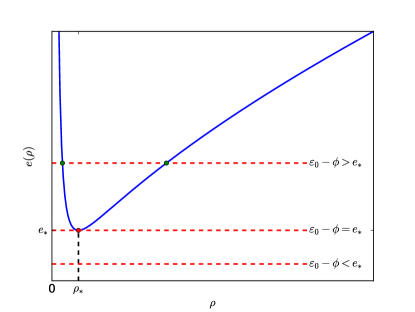
Figure 1: Sketch of the function $e(\rho)$ (Eq. 2.34). Also shown are the possibilities of no, one (red dot) and two solutions (green dots). In the case of two solutions, the left (right) solution with $\rho<\rho_{\ast}$ ($\rho>\rho_{\ast}$) is supersonic (subsonic).

So far, the discussion is applicable to any convex EoS. For ease of presentation, we assume an ideal gas law equation of state

$$p=(\gamma-1)\rho e,$$ (2.38)

where $\gamma$ is the ratio of specific heats. In that case, the equilibrium determination is simplified because $e_{\ast}$ can be computed explicitly. However, we stress that our well-balanced method is not restricted to this particular EoS and numerical experiments with a general convex EoS are shown in Section 3.3.

Thereby, we write the ideal gas law in the form

$$p=p(\rho,K)=K\rho^{\gamma},$$ (2.39)

where $K$ is a function of entropy alone, i.e. $K=K(s)$. Then we have $K_{0}=p_{0}/\rho_{0}^{\gamma}$ and consequently the critical values can be computed explicitly as

$$\rho_{\ast}=\left(\frac{m^{2}_{0}}{\gamma K_{0}}\right)^{\frac{1}{\gamma+1}},\;p_{\ast}=K_{0}\rho_{\ast}^{\gamma},\;v^{2}_{\ast}=c^{2}_{\ast}=\frac{\gamma p_{\ast}}{\rho_{\ast}},\;h_{\ast}=\frac{\gamma}{\gamma-1}\frac{p_{\ast}}{\rho_{\ast}}=\frac{c^{2}_{\ast}}{\gamma-1}\quad\text{and}\quad e_{\ast}=\frac{m^{2}_{0}}{2\rho_{\ast}}+h_{\ast}.$$ (2.40)

In case two equilibrium solutions exist, we chose the solution with sub/super-sonic velocity if the equilibrium constants correspond to a sub/super-sonic state. In practice, the equilibrium is found by a hybrid Newton method combining the quadratic convergence of the Newton method with a form of the robust bisection method, see e.g. [63]. The detailed algorithm is outlined in Algorithm 1.

Initial guess $\rho^{(0)}=\rho_{0}$;

for k = 0, 1, 2, … do

      if $\lvert e(\rho^{(k)})+\phi-\varepsilon_{0}\rvert<tol\leavevmode\nobreak\ e(\rho_{0})$ then Stop;

      $\rho^{(trial)}=\rho^{(k)}-\frac{e(\rho^{(k)})+\phi-\varepsilon_{0}}{e^{\prime}(\rho^{(k)})}$;

     

     if $v_{0}<c_{0}$ and $\rho^{(trial)}<\rho_{\ast}$ then  $\rho^{(trial)}=\frac{1}{2}(\rho_{\ast}+\rho^{(k)})$ ;

      if $v_{0}>c_{0}$ and $\rho^{(trial)}>\rho_{\ast}$  then  $\rho^{(trial)}=\frac{1}{2}(\rho^{(k)}+\rho_{\ast})$ ;

      if $\rho^{(trial)}<0$ then  $\rho^{(trial)}=\frac{1}{2}\rho_{(k)}$ ;

      $\rho^{(k+1)}=\rho^{(trial)}$;

     

      end for

Algorithm 1 Local equilibrium determination

The case of a general convex EoS is treated in the appendix, see Algorithm 2. This concludes the elaboration of the well-balanced scheme for one-dimensional steady adiabatic flow and we summarize it in the following:

Theorem 2.2.

Consider the scheme (2.3) with a consistent and Lipschitz continuous numerical flux $\mathcal{F}$, the spatially first/second-order reconstruction $\mathcal{W}$ (2.19)/(2.21) and source term discretization (2.28).

The scheme has the following properties:

1. The scheme is consistent with (2.1) and it is formally first/second-order accurate in space (for smooth solutions).

2. The scheme is well-balanced and preserves a discrete steady adiabatic flow given by (2.16) exactly.

Proof.

(i) The consistency and formal order of accuracy of the scheme is straightforward.

(ii) Let data $\boldsymbol{W}_{i}=[\rho_{i},v_{i},p_{i}]^{T}$ in steady adiabatic flow state (2.16) be given. Then both first- and second-order accurate reconstructions $\mathcal{W}$ (2.19)/(2.21) will yield the same equilibrium fulfilling state for the left and right cell interface traces

$$\boldsymbol{W}_{i+1/2-}=\boldsymbol{W}_{i+1/2+}=\boldsymbol{W}_{i+1/2}.$$

Plugging this into a consistent numerical flux gives

$$\boldsymbol{F}_{i+1/2}=\mathcal{F}(\boldsymbol{W}_{i+1/2},\boldsymbol{W}_{i+1/2})=\boldsymbol{f}(\boldsymbol{W}_{i+1/2}).$$

Similarly, we may evaluate the source term by Eq. 2.28

$$\boldsymbol{S}_{i}=\frac{1}{\Delta x}\begin{bmatrix}0\\ f^{(\rho v)}(\boldsymbol{W}_{i+1/2})-f^{(\rho v)}(\boldsymbol{W}_{i-1/2})\\ f^{(E)}(\boldsymbol{W}_{i+1/2})-f^{(E)}(\boldsymbol{W}_{i-1/2})\end{bmatrix}.$$

By combining both above expressions in (2.3), we immediately obtain

$$\frac{d}{dt}{}\boldsymbol{U}_{i}=\mathcal{L}(\boldsymbol{U}_{i})=-\frac{1}{\Delta x}\left(\boldsymbol{F}_{i+1/2}-\boldsymbol{F}_{i-1/2}\right)+\boldsymbol{S}_{i}=0.$$

This shows the well-balanced property of the scheme. $\blacksquare$

2.4 Extension to cylindrical and spherical symmetry

The Euler equations with gravity in cylindrical and spherical symmetry can be written in the following compact form

$$\partial_{t}\boldsymbol{u}+r^{-\alpha}\ \partial_{r}(r^{\alpha}\ \boldsymbol{f})=\boldsymbol{s}_{geo}+\boldsymbol{s}_{gra}=\boldsymbol{s}$$ (2.41)

where the conserved variables $\boldsymbol{u}$, the fluxes $\boldsymbol{f}$ and the gravity source term $\boldsymbol{s}_{gra}$ are as in Eq. 2.2. The radial coordinate is denoted by $r$ and $\alpha$ specifies whether the symmetry is cylindrical ($\alpha=1$) or spherical ($\alpha=2$). The geometric source term reads

$$\boldsymbol{s}_{geo}=\begin{bmatrix}0\\ \alpha r^{\alpha-1}p\\ 0\end{bmatrix}.$$ (2.42)

In these geometries, steady adiabatic flow is governed by

$$s=\text{const},\quad r^{\alpha}\rho v=\text{const}\quad\text{and}\quad\frac{v^{2}}{2}+h+\phi=\text{const}.$$ (2.43)

2.4.1 Standard finite-volume discretization

A semi-discrete finite volume method for Eq. 2.41 is given by

$$\frac{d}{dt}{}\boldsymbol{U}_{i}=\mathcal{L}(\boldsymbol{U})=-\frac{1}{\lvert V_{i}\rvert}\left(A_{i+1/2}\leavevmode\nobreak\ \boldsymbol{F}_{i+1/2}-A_{i-1/2}\boldsymbol{F}_{i-1/2}\right)+\boldsymbol{S}_{geo,i}+\boldsymbol{S}_{gra,i}.$$ (2.44)

where $V_{i}=[r_{i-1/2},r_{i+1/2}]$ denotes the $i$-th cell ranging over the left/right cell interface $r_{i\pm 1/2}=r_{i}\pm\Delta r/2$ with cell center $r_{i}$ and cell size $\Delta r$. Explicit expressions for the cell volume $\lvert V_{i}\rvert$ and interface areas $A_{i\pm 1/2}=A(r_{i\pm 1/2})$ are given by

$$\lvert V_{i}\rvert=2\pi\left(r_{i+1/2}^{2}-r_{i-1/2}^{2}\right),\quad A(r)=2\pi r$$ (2.45)

for cylindrical symmetry and

$$\lvert V_{i}\rvert=\frac{4\pi}{3}\left(r_{i+1/2}^{3}-r_{i-1/2}^{3}\right),\quad A(r)=4\pi r^{2}$$ (2.46)

for spherical symmetry.

For the numerical flux, reconstruction and gravity source term discretization, the same standard components as in the Cartesian case Section 2.1.1 can be employed. However, we note that specialized reconstruction procedures for curvilinear coordinates have been designed in the literature (see [64] and references therein).

The momentum component of the geometric source term $\boldsymbol{s}_{geo}$ can be discretized as

$$S^{(\rho v)}_{geo,i}=\frac{1}{\lvert V_{i}\rvert}\left(A_{i+1/2}-A_{i-1/2}\right)p_{i},$$ (2.47)

where $p_{i}$ is the pressure at cell center, or more precisely, computed simply from the cell-averaged conserved variables $\boldsymbol{W}_{i}=\boldsymbol{w}(\boldsymbol{U}_{i})$. Note that this discretization has the desirable property that resting uniform conditions ($\rho=\text{const}$, $p=\text{const}$ and $v=0$) are exactly preserved.

In general, the just outlined standard finite volume scheme for cylindrical/spherical symmetry has difficulties in resolving the steady adiabatic equilibrium Eq. 2.43. Next, we describe the necessary modifications enabling the scheme to exactly preserve such steady states, thereby extending the approach of Cartesian geometry from Section 2.2.

2.4.2 Well-balanced finite-volume discretization

We follow the structure in the section of well-balanced finite volume discretization in Cartesian coordinates and will first describe the finite volume method in terms of an abstract equilibrium reconstruction, i.e. for each cell let $\boldsymbol{W}_{eq,i}=(\rho_{eq,i},v_{eq,i},p_{eq,i})$ be a stationary solution of the Euler equation in cylindrical and spherical symmetry satisfying Eq. 2.43 such that $\boldsymbol{W}_{eq,i}=\boldsymbol{W}_{i}$. In a second step we will describe how to evaluate $\boldsymbol{W}_{eq,i}$.

Reconstruction

The well-balanced reconstruction Section 2.2.1, based on equilibrium profiles which satisfy Eq. 2.43 can also be used in cylindrical and spherical coordinates.

Momentum source term

The derivation of the momentum source term in cylindrical and spherical coordinates closely follows Section 2.2.2. However, in curvilinear coordinates we need to additionally consider the geometric source term, i.e.

$$\frac{1}{r^{\alpha}}\partial_{r}r^{\alpha}\boldsymbol{f}^{(\rho v)}(\boldsymbol{W}_{eq,i})=\boldsymbol{s}_{geo}(\boldsymbol{W}_{eq,i})+\boldsymbol{s}_{gra}(\boldsymbol{W}_{eq,i})=\alpha r^{\alpha-1}p_{eq,i}-\rho_{eq,i}\partial_{r}{\phi}.$$ (2.48)

In a first step, we split the pressure and density into an equilibrium and perturbation term as follows

$$\boldsymbol{s}_{geo}^{(\rho v)}(r,\boldsymbol{W}_{i}(r))+s_{gra}^{(\rho v)}(r,\boldsymbol{W}_{i}(r))=\alpha r^{\alpha-1}(p_{eq,i}(r)+\delta p_{i}(r))-(\rho_{eq,i}(r)+\delta\rho_{i}(r))\ \partial_{r}\phi.$$ (2.49)

By the same steps as in the Cartesian case, the well-balanced cell-averaged source term in cell $V_{i}$ is determined to be

$$S_{i}^{(\rho v)} =\frac{1}{\lvert V_{i}\rvert}\left.A(r)\left(\rho v^{2}_{eq,i}(r)+p_{eq,i}(r)\right)\right|^{r_{i+1/2}}_{r_{i-1/2}}.$$ (2.50)

Energy source term discretization

The derivation of the energy source term also closely follows its Cartesian counter part. Following those steps, we derive that up to second order

$$s^{(E)}(r,\boldsymbol{W}_{i}(r)) =\frac{1}{r^{\alpha}}\partial_{r}(r^{\alpha}f^{(E)}(\boldsymbol{W}_{eq,i})).$$ (2.51)

The well-balanced energy source term is obtained in a similar fashion as the momentum source term and reads

$$S_{i}^{(E)}=\frac{1}{\lvert V_{i}\rvert}\left.A(r)f^{(E)}(\boldsymbol{W}_{eq,i})\right|_{r_{i-1/2}}^{r_{i+1/2}}.$$ (2.52)

2.4.3 Local equilibrium reconstruction in cylindrical/spherical symmetry

In analogy to the equilibrium reconstruction in Cartesian coordinates, we formally define an equilibrium profile $\boldsymbol{W}_{eq,i}(r)$ which satisfies the equations of steady adiabatic flow in cylindrical and spherical coordinates. The only difference is the mass flux which accounts for the geometry

$$r^{\alpha}\rho_{eq,i}(r)v_{eq,i}(r)=r^{\alpha}_{i}\rho_{i}v_{i}=m_{i},$$ (2.53)

where we again fix the constant by their values at cell center $r_{i}$. Following precisely the steps outlined in Section 2.3, we obtain one scalar equation for the equilibrium density, namely

$$\frac{m_{i}^{2}}{2r^{2\alpha}\rho^{2}_{eq,i}(r)}+h(p_{eq,i}(r),s_{eq,i}(r))+\phi(r)=\varepsilon_{i}.$$ (2.54)

Let us again simplify notation by rewriting Eq. 2.54 as

$$\frac{m_{0}^{2}}{2r^{2\alpha}\rho^{2}}+h(p(\rho,s_{0}),s_{0})+\phi(r)=\varepsilon_{0}.$$ (2.55)

where $m_{0}$, $s_{0}$ and $\varepsilon_{0}$ denote the values of $m$, $s$ and $\varepsilon$ at a reference point $r_{0}$. The corresponding thermodynamic part and its derivative are

$$e(\rho,r)=\frac{m_{0}^{2}}{2r^{2\alpha}\rho^{2}}+h(\rho),\quad e^{\prime}(\rho,r)=-\frac{m_{0}^{2}}{2r^{2\alpha}\rho^{3}}+\frac{c^{2}(\rho)}{\rho}.$$ (2.56)

Both now depend on the spatial coordinate $r$. Let $\rho_{\ast}$ be the critical density such that $e^{\prime}(\rho,r)=0$. Clearly, both the $\rho_{\ast}$ and $e_{\ast}$ are functions of $r$. Keeping this fact in mind, we determine the number of solutions to Eq. 2.54 as in the Cartesian case.

The same hybrid Newton’s method proposed for the Cartesian case (Algorithm 1), can be used to solve Eq. 2.56. However, since $\rho_{\ast}$ now depends on $r$, it could happen that the reference state is on the supersonic branch $\rho_{0}<\rho_{\ast}(r_{0})$, but the initial guess given to the algorithm $\rho^{(0)}=\rho_{0}$ is on the subsonic branch $\rho_{0}>\rho_{\ast}(r)$, or vice versa. Therefore, we choose the initial guess as follows

$$\rho^{(0)}=\frac{\rho_{0}}{\rho_{\ast}(r_{0})}\rho_{\ast}(r),$$ (2.57)

which ensures that the initial guess is in the same sub-/super-sonic regime as the reference state.

This concludes the elaboration of the well-balanced scheme for steady adiabatic flow in cylindrical and spherical coordinates. We summarize the schemes’ properties in the following:

Corollary 2.3.

Consider the scheme (2.44) with a consistent and Lipschitz continuous numerical flux function $\mathcal{F}$, the spatially first/second-order accurate reconstruction $\mathcal{W}$ Eq. 2.19/Eq. 2.21 and source term discretization Eq. 2.50 and Eq. 2.52.

The scheme has the following properties:

1. The scheme is consistent with (2.41) and it is formally first/second-order in space (for smooth solutions).

2. The scheme is well-balanced and preserves a discrete steady adiabatic flow given by (2.43) exactly.

Proof.

The proof parallels mostly the one of Theorem 2.2 and is straightforward. $\blacksquare$

2.5 Extension to several space dimensions

We briefly outline the straightforward extension of the above schemes to several space dimensions. However, the extension will in general only be truly well-balanced if the streamlines of the steady adiabatic flow of interest are aligned with a computational grid axis.

For the sake of simplicity, we treat the two-dimensional Cartesian case explicitly since the extension to other geometries and three dimensions is analogous. The two-dimensional Euler equations with gravity in Cartesian coordinates are given by

$$\partial_{t}\boldsymbol{u}+\partial_{x}\boldsymbol{f}+\partial_{y}\boldsymbol{g}=\boldsymbol{s}$$ (2.58)

with

$$\boldsymbol{u}=\begin{bmatrix}\rho\\ \rho v_{x}\\ \rho v_{y}\\ E\end{bmatrix},\quad\boldsymbol{f}=\begin{bmatrix}\rho v_{x}\\ \rho v_{x}^{2}+p\\ \rho v_{y}v_{x}\\ (E+p)v_{x}\end{bmatrix},\quad\boldsymbol{g}=\begin{bmatrix}\rho v_{y}\\ \rho v_{x}v_{y}\\ \rho v_{y}^{2}+p\\ (E+p)v_{y}\end{bmatrix}\quad\mathrm{and}\quad\boldsymbol{s}=\boldsymbol{s}^{x}+\boldsymbol{s}^{y}=-\begin{bmatrix}0\\ \rho\\ 0\\ \rho v_{x}\end{bmatrix}\partial_{x}\phi-\begin{bmatrix}0\\ 0\\ \rho\\ \rho v_{y}\end{bmatrix}\partial_{y}{\phi},$$ (2.59)

where $\boldsymbol{u}$ is the vector of conserved variables, $\boldsymbol{f}$ and $\boldsymbol{g}$ the fluxes in $x$- and $y$-direction, and $\boldsymbol{s}$ the gravitational source terms. The primitive variables are given by $\boldsymbol{w}=[\rho,v_{x},v_{y},p]^{T}$.

We consider a rectangular spatial domain $\Omega=[x_{\min},x_{\max}]\times[y_{\min},y_{\max}]$ discretized uniformly (for ease of presentation) by $N_{x}$ and $N_{y}$ cells or finite volumes in $x$- and $y$-direction, respectively. The cells are labeled by $I_{i,j}=I_{i}\times I_{j}=[x_{i-1/2},x_{i+1/2}]\times[y_{j-1/2},y_{j+1/2}]$ and the constant cell sizes by $\Delta x=x_{i+1/2}-x_{i-1/2}$ and $\Delta y=y_{j+1/2}-y_{j-1/2}$. We denote the cell centers by $x_{i}=(x_{i-1/2}+x_{i+1/2})/2$ and $y_{j}=(y_{j-1/2}+y_{j+1/2})/2$.

A semi-discrete finite volume scheme for the numerical approximation of (2.58) then takes the following form

$$\frac{\mathrm{d}}{\mathrm{d}t}\boldsymbol{U}_{i,j}=\mathcal{L}(\boldsymbol{U})=-\frac{1}{\Delta x}\left(\boldsymbol{F}_{i+1/2,j}-\boldsymbol{F}_{i-1/2,j}\right)-\frac{1}{\Delta y}\left(\boldsymbol{G}_{i,j+1/2}-\boldsymbol{G}_{i,j-1/2}\right)+\boldsymbol{S}_{i,j},$$ (2.60)

where $\boldsymbol{U}_{i,j}$ denotes the approximate cell averages of the conserved variables,

$$\boldsymbol{F}_{i\pm 1/2,j}=\mathcal{F}(\boldsymbol{W}_{i\pm 1/2-,j},\boldsymbol{W}_{i\pm 1/2+,j})\quad\text{and}\quad\boldsymbol{G}_{i,j\pm 1/2}=\mathcal{G}(\boldsymbol{W}_{i,j\pm 1/2-},\boldsymbol{W}_{i,j\pm 1/2+})$$ (2.61)

the numerical fluxes through the respective cell face, and $\boldsymbol{S}_{i,j}$ the cell averages of the source term. The $\boldsymbol{W}_{i\pm 1/2\mp,j}$ and $\boldsymbol{W}_{i,j\pm 1/2\mp}$ denote the traces of the primitive variables at the center of the cell face, in the respective direction.

The equilibrium preserving reconstruction $\mathcal{W}$ of Section 2.2.1 is trivially applied in $x$- and $y$-direction independently. In $x$-direction, let

$$\boldsymbol{W}^{x}_{eq,i,j}(x)=\left(\rho^{x}_{eq,i,j}(x),v^{x}_{x,eq,i,j}(x),0,p^{x}_{eq,i,j}(x)\right)$$ (2.62)

be the solution of

$$s=\text{const},\quad\rho v_{x}=\text{const},\quad\frac{v_{x}^{2}}{2}+h+\phi=\text{const},$$ (2.63)

as described in Section 2.3. The well-balanced reconstruction in $x$-direction is then

$$\boldsymbol{W}_{i,j}(x,y_{j})=\mathcal{W}^{x}\left(x,y_{j};\left\{\boldsymbol{W}_{k,j}\right\}_{k\in S_{i}}\right)=\boldsymbol{W}^{x}_{eq,i,j}(x)+\delta^{x}\boldsymbol{W}_{i,j}(x,y_{j}).$$ (2.64)

Note that since the transverse component of the velocity of $\boldsymbol{W}^{x}_{eq,i,j}$ is zero, the reconstruction of that component of the velocity is in fact simply the standard reconstruction. The reconstruction in $y$-direction is obtained by simply reversing the roles of $v_{x}$ and $v_{y}$.

The gravity source terms are discretized as

$$\boldsymbol{S}_{i,j}=\boldsymbol{S}^{x}_{i,j}+\boldsymbol{S}^{y}_{i,j},\quad\boldsymbol{S}^{x}_{i,j}=\begin{bmatrix}0\\ S^{x,(\rho v_{x})}_{i,j}\\ 0\\ S^{x,(E)}_{i,j}\end{bmatrix}\quad\text{and}\quad\boldsymbol{S}^{y}_{i,j}=\begin{bmatrix}0\\ 0\\ S^{y,(\rho v_{y})}_{i,j}\\ S^{y,(E)}_{i,j}\end{bmatrix}.$$ (2.65)

The momentum source term is computed by Eq. 2.26 on a dimension-by-dimension basis as

$$S^{x,(\rho v_{x})}_{i,j}=\left.\frac{1}{\Delta x}f^{(\rho v_{x})}\left(\boldsymbol{W}^{x}_{eq,i,j}(x,y_{j})\right)\right|_{x_{i-1/2}}^{x_{i+1/2}}\quad\text{and}\quad S^{y,(\rho v_{y})}_{i,j}=\left.\frac{1}{\Delta y}g^{(\rho v_{y})}\left(\boldsymbol{W}^{y}_{eq,i,j}(x_{i},y)\right)\right|_{y_{j-1/2}}^{y_{j+1/2}}.$$ (2.66)

Likewise, the energy source term is computed by Eq. 2.27 on a dimension-by-dimension basis as

$$S^{x,(E)}_{i,j}=\left.\frac{1}{\Delta x}f^{(E)}\left(\boldsymbol{W}^{x}_{eq,i,j}(x,y_{j})\right)\right|_{x_{i-1/2}}^{x_{i+1/2}}\quad\text{and}\quad S^{y,(E)}_{i,j}=\left.\frac{1}{\Delta y}g^{(E)}\left(\boldsymbol{W}^{y}_{eq,i,j}(x_{i},y)\right)\right|_{y_{j-1/2}}^{y_{j+1/2}}.$$ (2.67)

This concludes the outline of the extension of the well-balanced schemes to multiple dimensions. It is clear that it is well-balanced if the streamlines of the considered steady state are aligned with the $x$- or $y$-axis.

3 Numerical Experiments

In this section, we test our well-balanced schemes on a series of numerical experiments and compare their performance with a standard (unbalanced) base scheme. Furthermore, we also compare to the hydrostatically well-balanced scheme [21]. For the sake of conciseness, we only present the results for the practically relevant second-order schemes.

To characterize a time scale on which a model reacts to perturbations of its equilibrium, we define a characteristic crossing time

$$\tau_{\mathrm{char}}=\int_{x_{0}}^{x_{1}}\frac{\mathrm{d}x}{\lvert v\rvert+c},$$ (3.1)

where $v$ is the fluid velocity and $c$ the sound speed. It measures the time it takes a wave traveling at the fastest characteristic speed to traverse the steady state of interest.

We quantify the accuracy of the schemes by computing the absolute errors

$$err_{1}(q)=\|q-q_{ref}\|_{1},$$ (3.2)

where $\|.\|_{1}$ denotes the 1-norm, $q$ some quantity of interest (e.g. pressure, velocity, …) and $q_{ref}$ a reference solution. The reference solution may be the steady state to be maintained discretely or the result of an appropriately averaged high-resolution simulation. While the comparison with a numerically obtained reference solution does not provide a rigorous evidence of convergence, it nevertheless indicates a meaningful measure of the errors. We also introduce the following relative error measure

$$relerr_{1}(q)=\frac{\|q-q_{ref}\|_{1}}{\|q_{ref}\|_{1}}.$$ (3.3)

We begin in Section 3.1 by several simple one-dimensional numerical experiments with Cartesian geometry followed in Section 3.2 by several simple one-dimensional numerical experiments with spherical geometry. Both setups employ an ideal gas EoS. The interested reader may readily reproduce these experiments in order to check his or her implementation. Finally, we demonstrate in Section 3.3 the performance of the scheme on a two-dimensional stellar accretion problem in cylindrical coordinates involving a complex multi-physics EoS.

3.1 One-dimensional steady adiabatic flow

The first and simplest test we perform is a steady state solution of Eq. 1.1 in Cartesian coordinates on the domain $\Omega=[0,2]$ with and without a perturbation. The gravity is given by a linear gravitational potential, i.e. $\phi(x)=gx$, with $g=1$. The ratio of specific heats is $\gamma=5/3$. We enforce boundary conditions by keeping the values in the ghost-cells constant and equal to the initial conditions. All numerical solvers in this subsection use the HLLC numerical flux and the monotonized centered limiter. The tolerance in the root finding procedure Algorithm 1 is $tol=10^{-13}$. The CFL number is $c_{CFL}=0.45$.

The initial conditions are

$$\left(\rho^{0},v^{0},p^{0}\right)(x)=\left(\rho_{eq}(x),v_{eq}(x),p_{eq}(x)+A\exp(-(x-\bar{x})^{2}/\sigma^{2})\right)$$ (3.4)

where $\sigma=0.1$, $\bar{x}$ is the center of the bump and $(\rho_{eq},v_{eq},p_{eq})$ is the equilibrium defined by the points values

$$(\rho_{0},v_{0},p_{0})=(1,-Mc_{s,0},1)$$ (3.5)

at $x_{0}=0$. Here $c_{s,0}=\gamma^{1/2}$ denotes the speed of sound at $x_{0}$. The discrete initial conditions are obtained by applying the midpoint rule to Eq. 3.4 which results in

$$\left(\rho_{i}^{0},v_{i}^{0},p_{i}^{0}\right)=\left(\rho^{0}(x_{i}),v^{0}(x_{i}),p^{0}(x_{i})\right).$$ (3.6)

We perform the experiment for a hydrostatic ($M=0$), a subsonic ($M=0.01$) and a supersonic ($M=2.5$) equilibrium and different sizes of the perturbation (specified later) will be investigated. The location of the perturbation is

$$\bar{x}=\begin{cases}1.0,&\text{for }M=0\\ 1.1,&\text{for }M=0.01\\ 1.5,&\text{for }M=2.5.\end{cases}$$ (3.7)

All convergence studies in this subsection are run with the unbalanced, hydrostatically well-balanced and adiabatically well-balanced schemes on $N=32,64,128,\dots,$2048$$ cells. A reference solution is computed by the adiabatically well-balanced method on $N=8192$ cells.

3.1.1 Well-balanced property

In this first experiment, we set the amplitude of the perturbation to zero and check that the proposed scheme is well-balanced for all three values of $M$. The simulation is run until $t_{f}=4$ ($M<1$) or $t_{f}=1$ ($M>1$) which corresponds to roughly two characteristic crossing times $\tau_{\mathrm{char}}$.

The results are shown in Table 7. For all values of $M$ the adiabatically well-balanced method preserves the discrete stationary state down to machine precision. As expected, the hydrostatically well-balanced method only preserves the hydrostatic case where $M=0$. Finally, the unbalanced scheme produces large errors and is unable to maintain the steady state accurately.

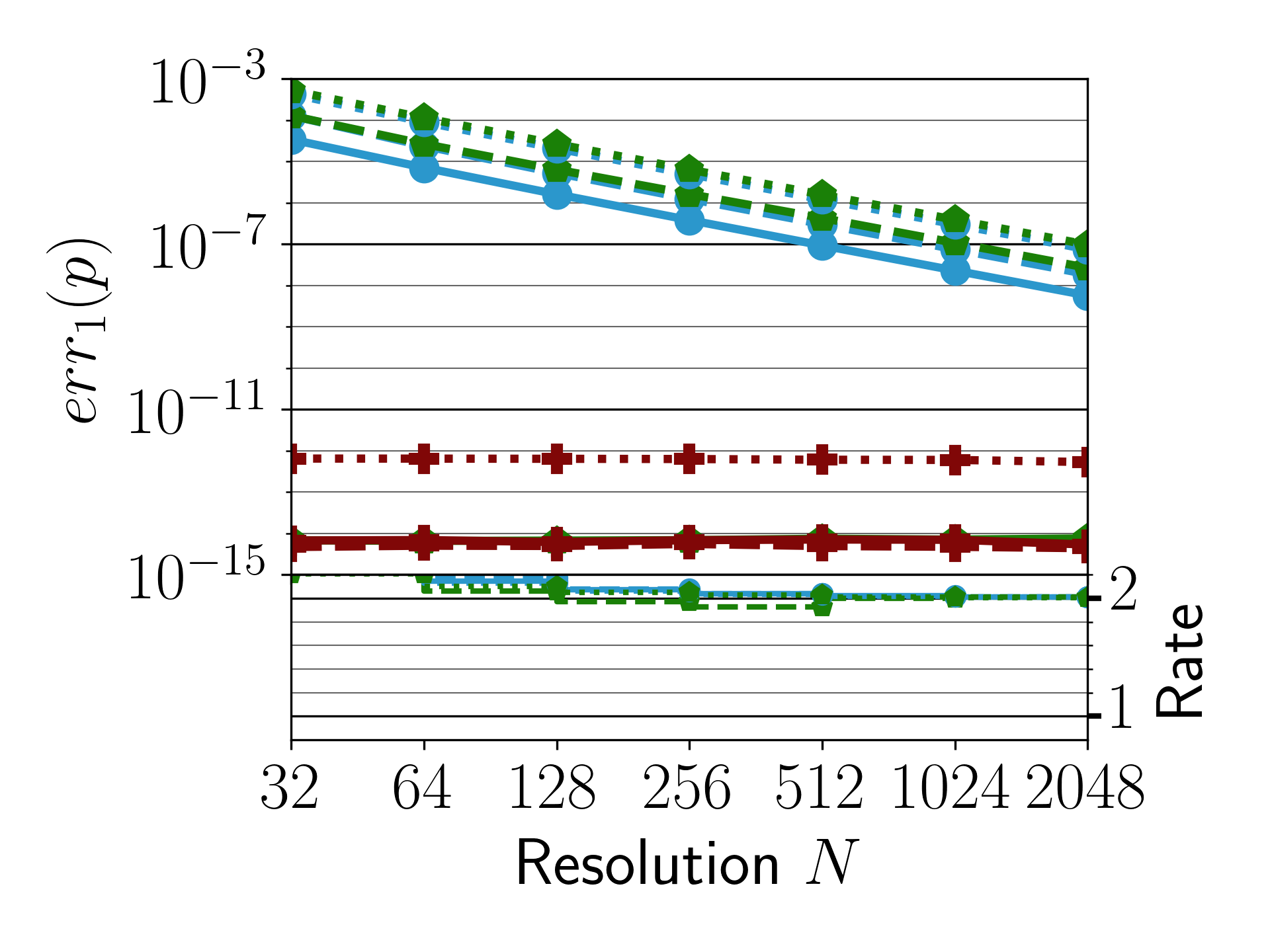
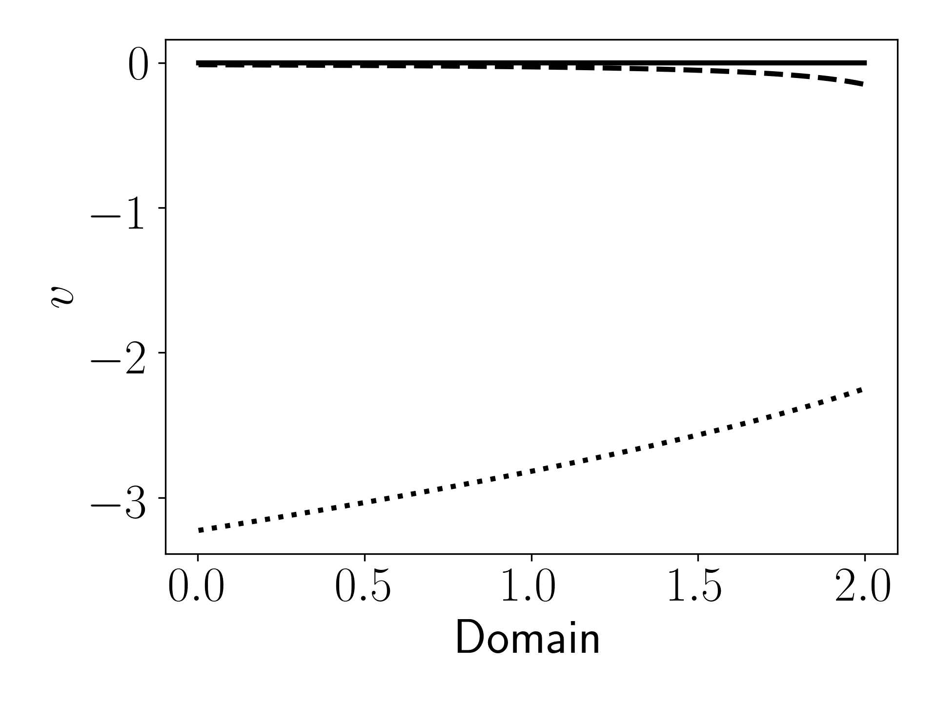
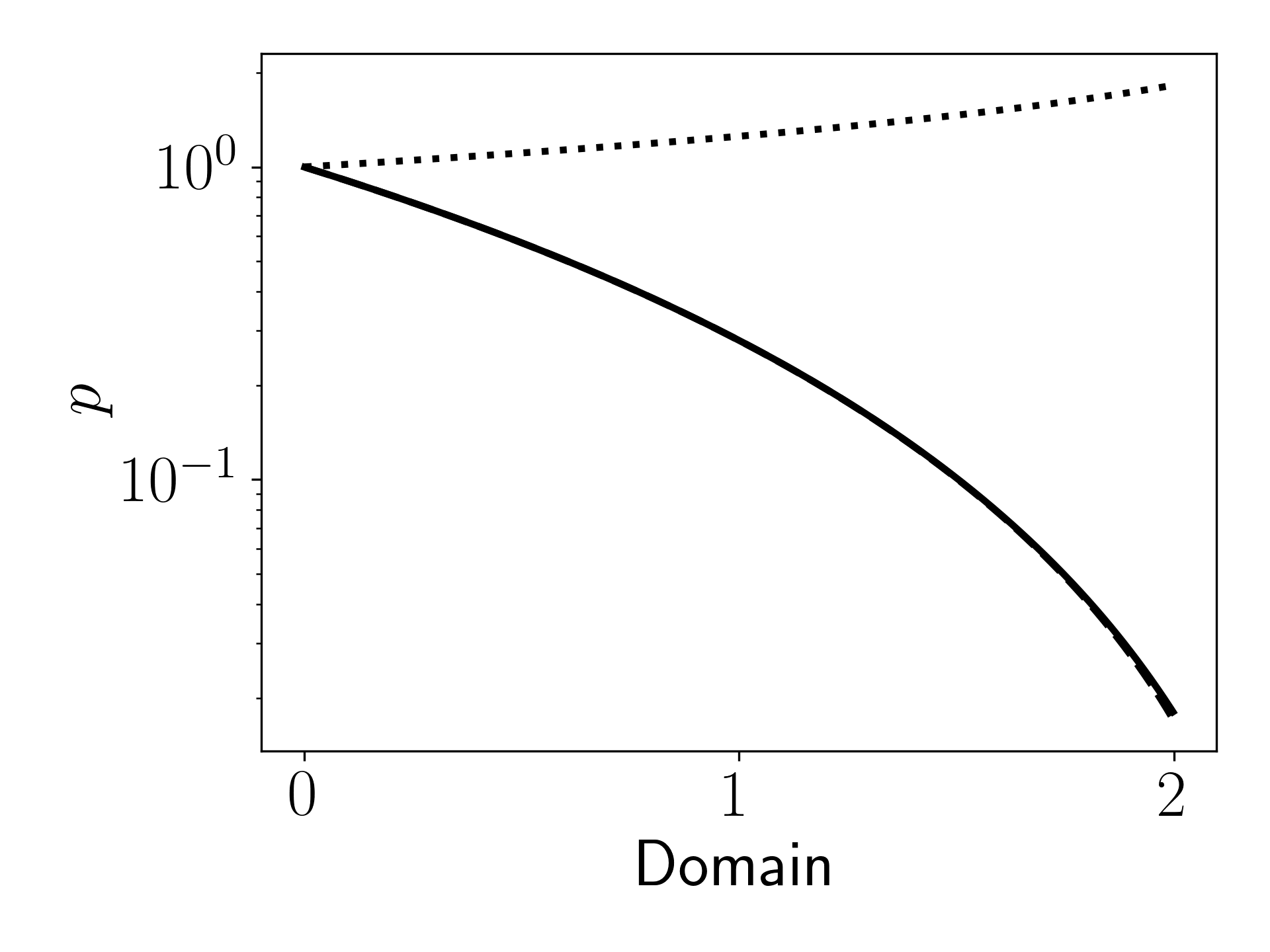
Figure 2: The left most column shows the well-balanced property of the methods on the problem described in Section 3.2.1 (with $A=0$). The upper part of the subplot shows the $L^{1}$-error of the pressure $p$. The lower subplot shows the convergence rate between two consecutive levels of refinement. The unbalanced, hydrostatically well-balanced and adiabatically well-balanced scheme is shown in blue, green and red, respectively. The solid black line is the reference solution. The middle column shows the velocity and the right column shows the pressure, both at $t_{f}=0$. Solid, dash and dotted lines represent $M=0$, $M=0.01$ and $M=2.5$ cases, respectively. Note that the pressure for the hydrostatic and subsonic cases nearly coincide.

3.1.2 Smooth wave propagation

We now compare the ability of the schemes to propagate small perturbations on top of the equilibrium. The size of the perturbation, $A=10^{-6}$, is chosen such that the wave remains smooth for the duration of the numerical experiment.

The results at $t_{f}=0.45$ ($M<1$) or $t_{f}=0.25$ ($M>1$) are shown in Figs. 3, 4 and 5 and Table 8 is the corresponding convergence table. All three solvers attain their formal second-order accuracy. The adiabatically well-balanced method is the only scheme capable of evolving the pressure perturbation accurately for all Mach numbers and for $M>0$ the error is smaller by a factor of at least $100$ compared to the hydrostatically well-balanced method. The hydrostatically well-balanced method coincides with the adiabatically well-balanced method for $M=0$. At $M=0.01$ the hydrostatically well-balanced method is only slightly better than the unbalanced solver. For $M=2.5$ the hydrostatically well-balanced method has lost its advantage over the unbalanced solver. We highlight that the errors of the adiabatically well-balanced scheme at the lowest resolutions $N=32,64$ are comparable to the errors of the unbalanced scheme at the highest resolution $N=2048$ for all velocities.

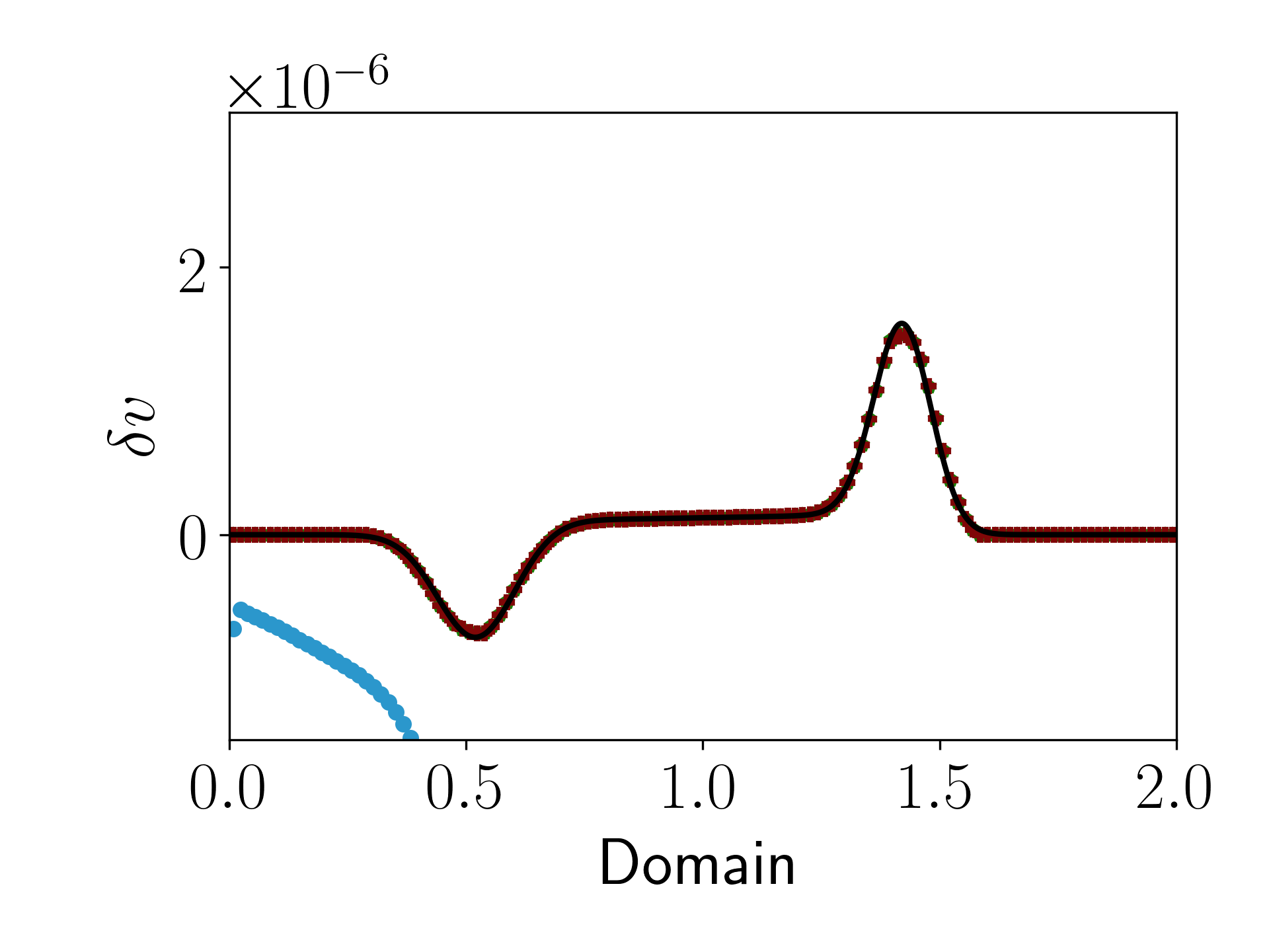
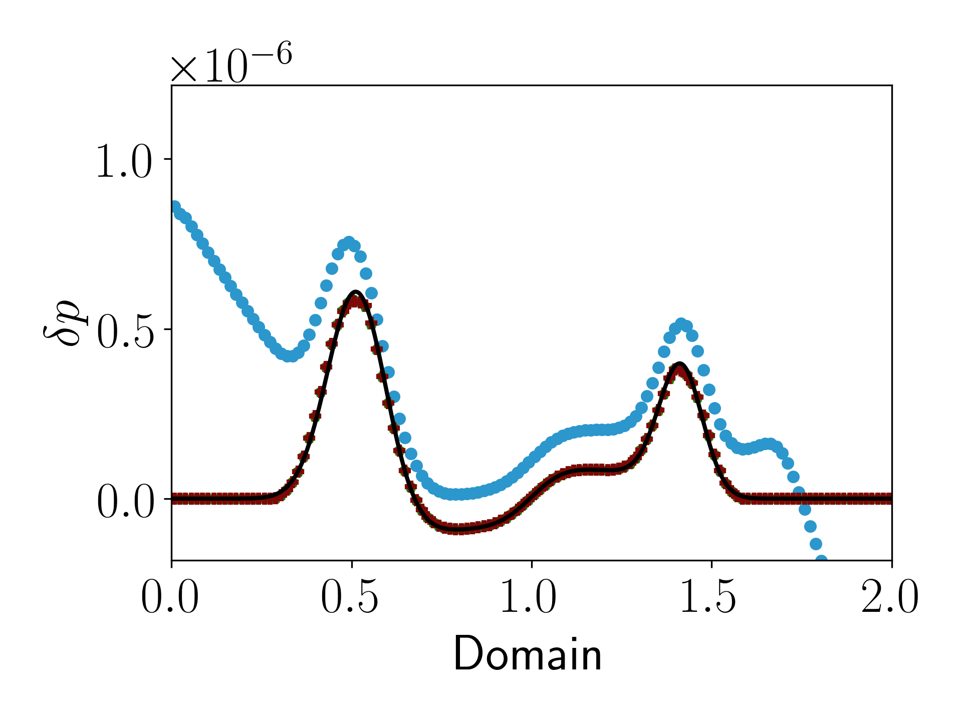
Figure 3: The left most column shows the convergence of the methods on the problem described in Section 3.1 with $A=10^{-6}$. The upper part of the subplot shows the $L^{1}$-error of the pressure perturbation $\delta p$. The lower subplot shows the convergence rate between two consecutive levels of refinement. The middle column shows the velocity perturbation $\delta v$ and the right column shows the pressure perturbation $\delta p$. The Mach number at the reference point is $M=0$. The scatter plots show the approximation with $N=128$ cells at the final time described in the text. The unbalanced, hydrostatically well-balanced and adiabatically well-balanced scheme is shown in blue, green and red, respectively. The solid black line is the reference solution.

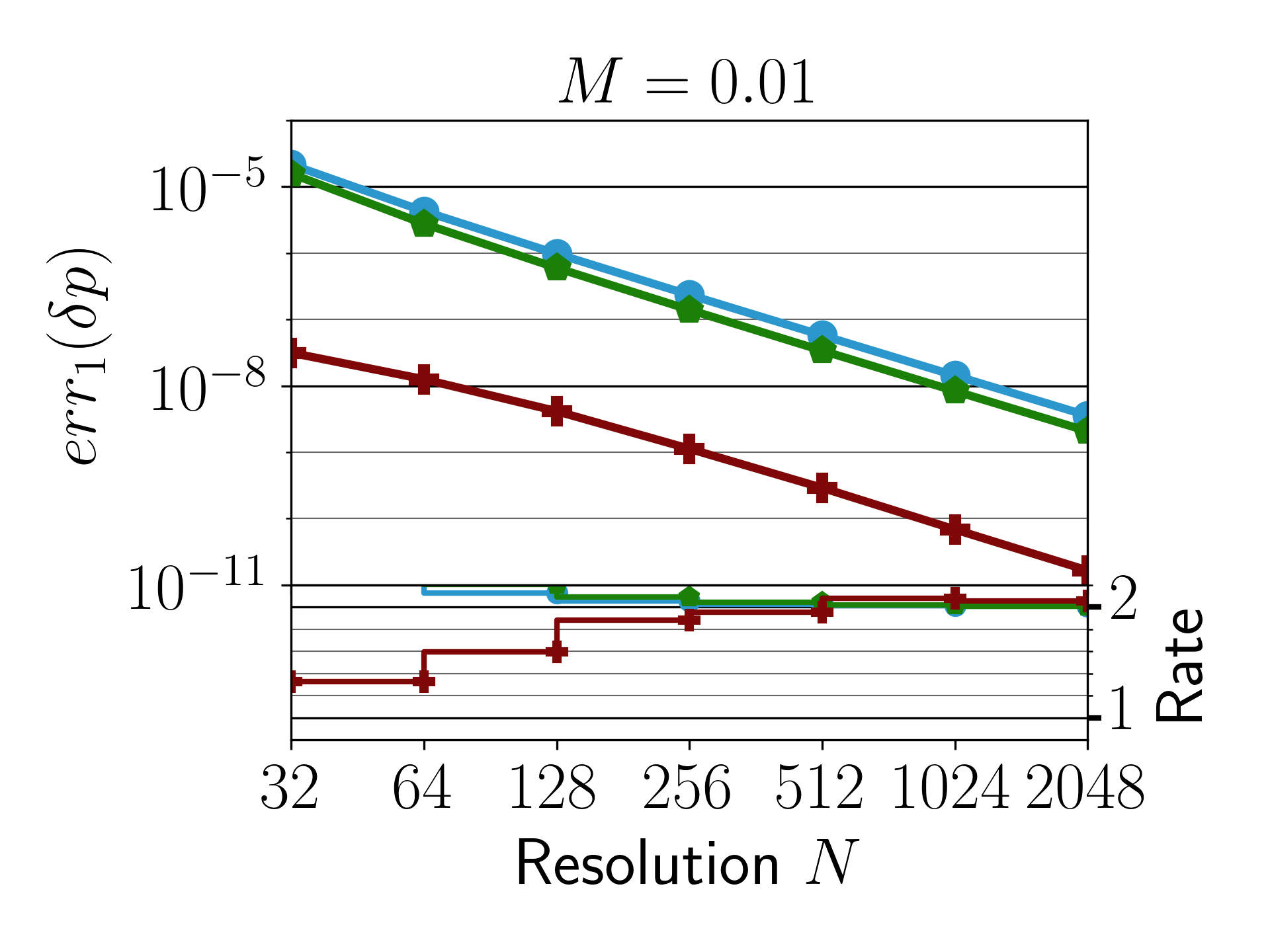
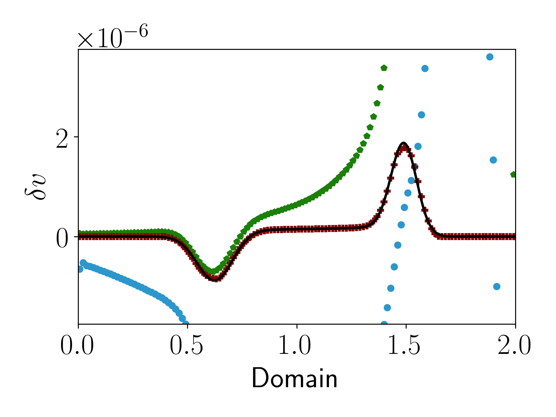
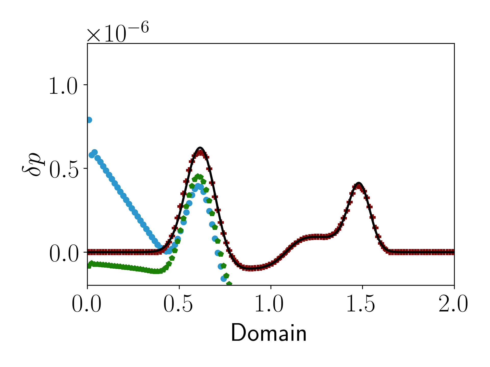
Figure 4: This figure shows the results for Section 3.1 with $A=10^{-6}$ and $M=0.01$. Please refer to the caption of Fig. 3 for further details.

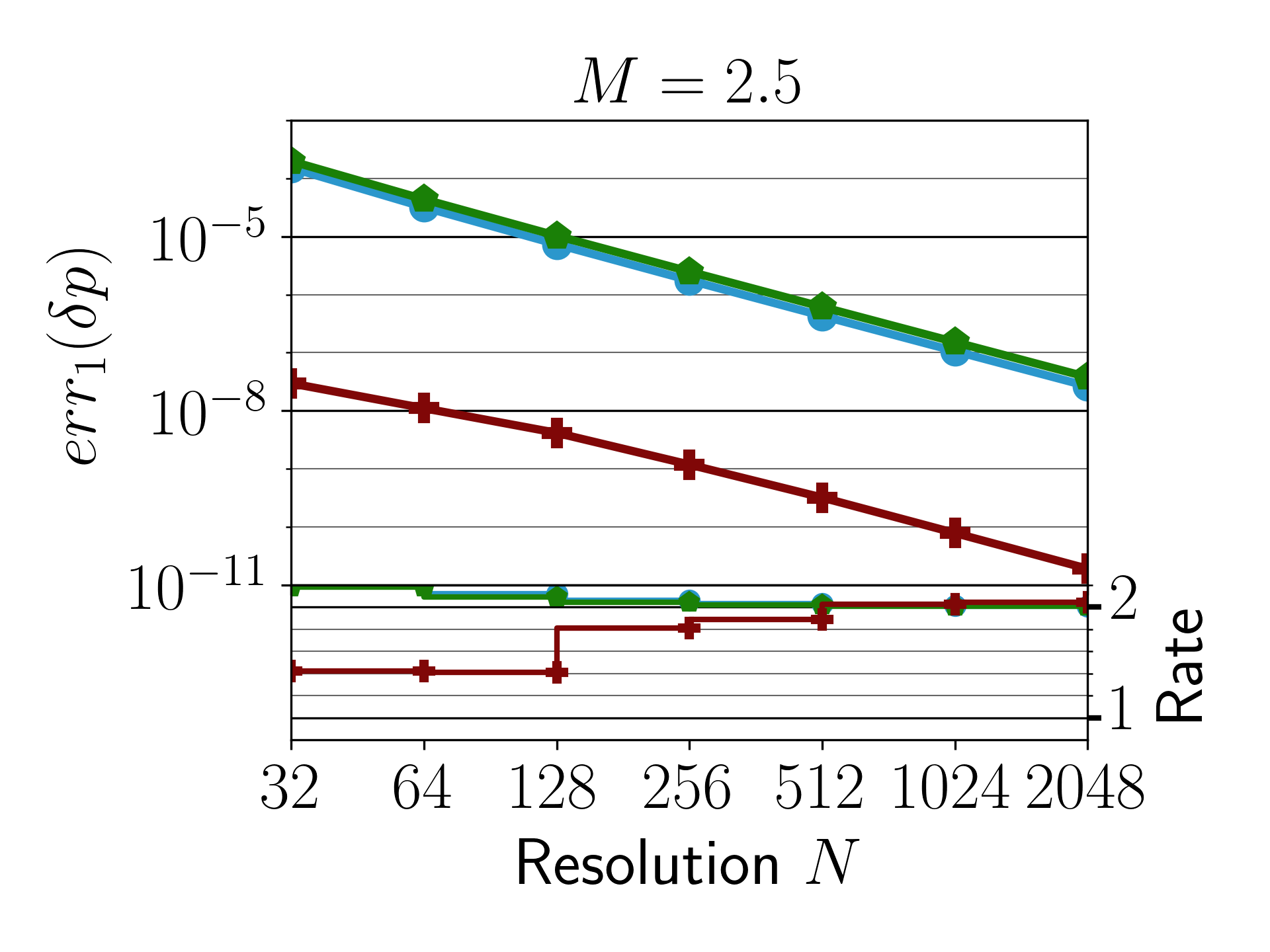
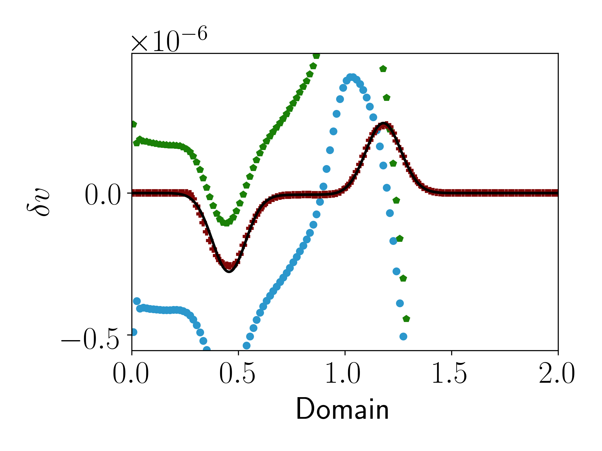
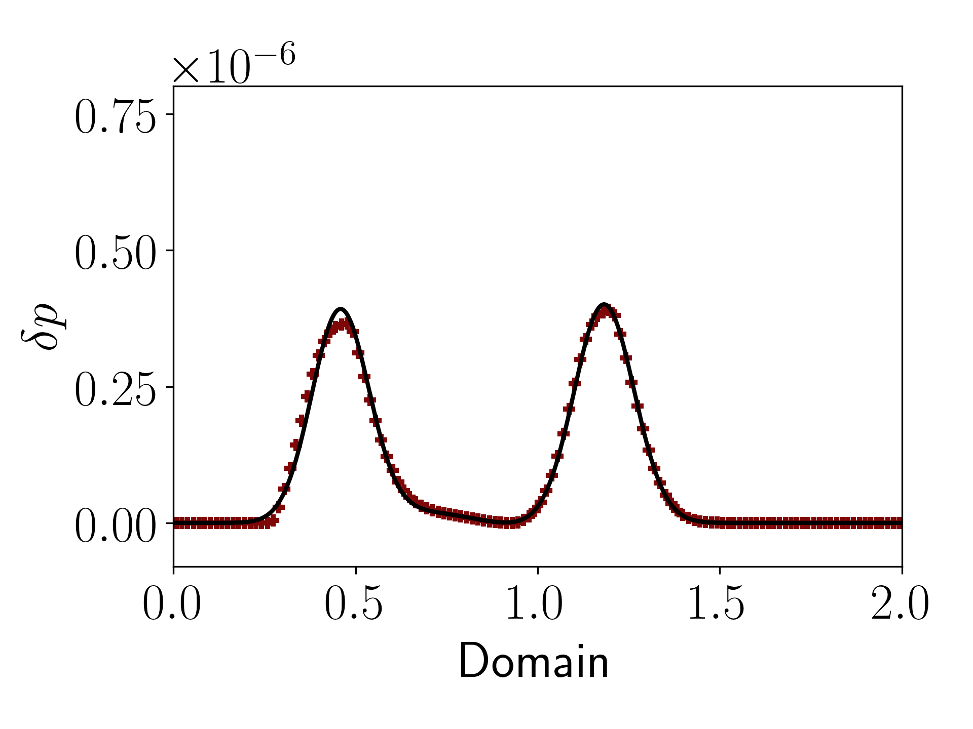
Figure 5: This figure shows the results for Section 3.1 with $A=10^{-6}$ and $M=2.5$. Please refer to the caption of Fig. 3 for further details.

3.1.3 Discontinuous wave propagation

In this third variant of the numerical experiment, we choose the magnitude of the pressure perturbation such that due to the non-linearity of the Euler equations the solution becomes discontinuous before the end of the simulation, which is chosen to be $t_{f}=0.45$ ($M<1$) or $t_{f}=0.25$ ($M>1$).

The results for $M=0.01$ are summarized in Fig. 6 and in the corresponding convergence table, Table 9. Numerically, we observe that all three methods are able to propagate the shock waves. In fact, they are virtually indistinguishable. Therefore, we observe that the well-balancing does not impact on the robustness of the base high resolution shock-capturing finite volume scheme. The observed convergence rate of approximately one is expected for solutions with an isolated discontinuity.

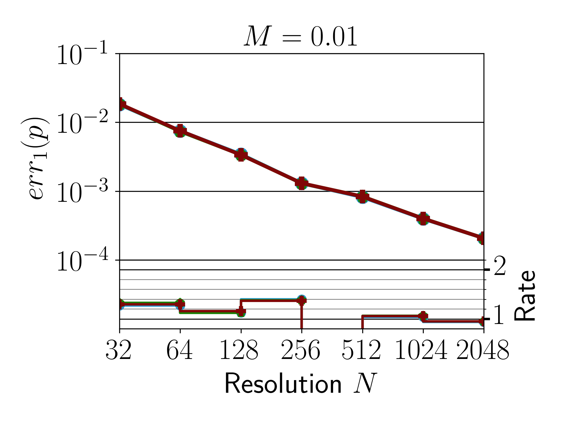
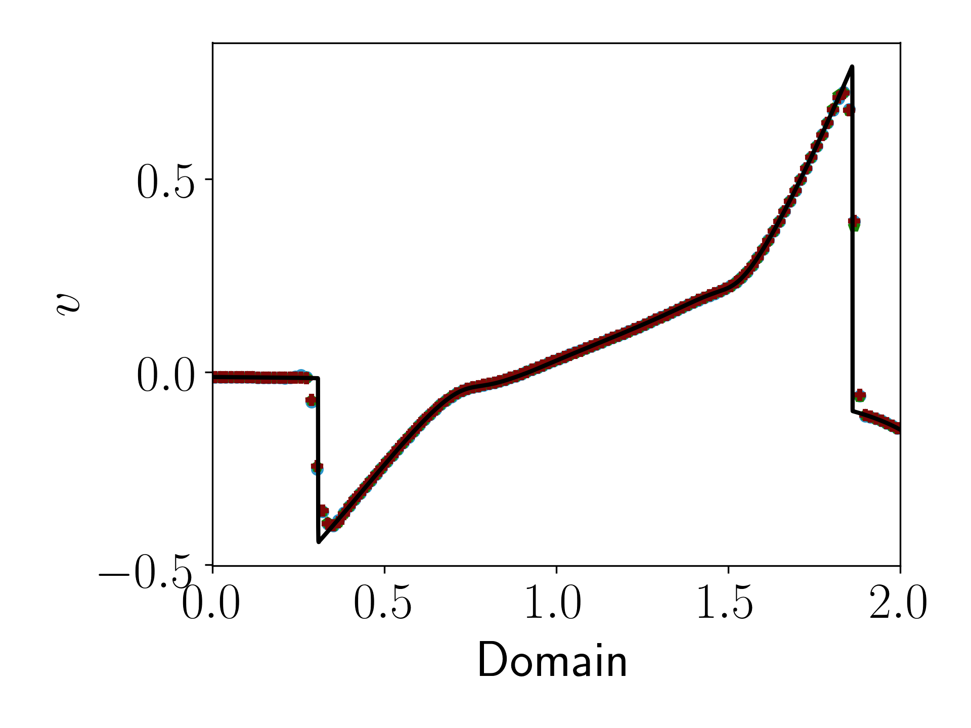
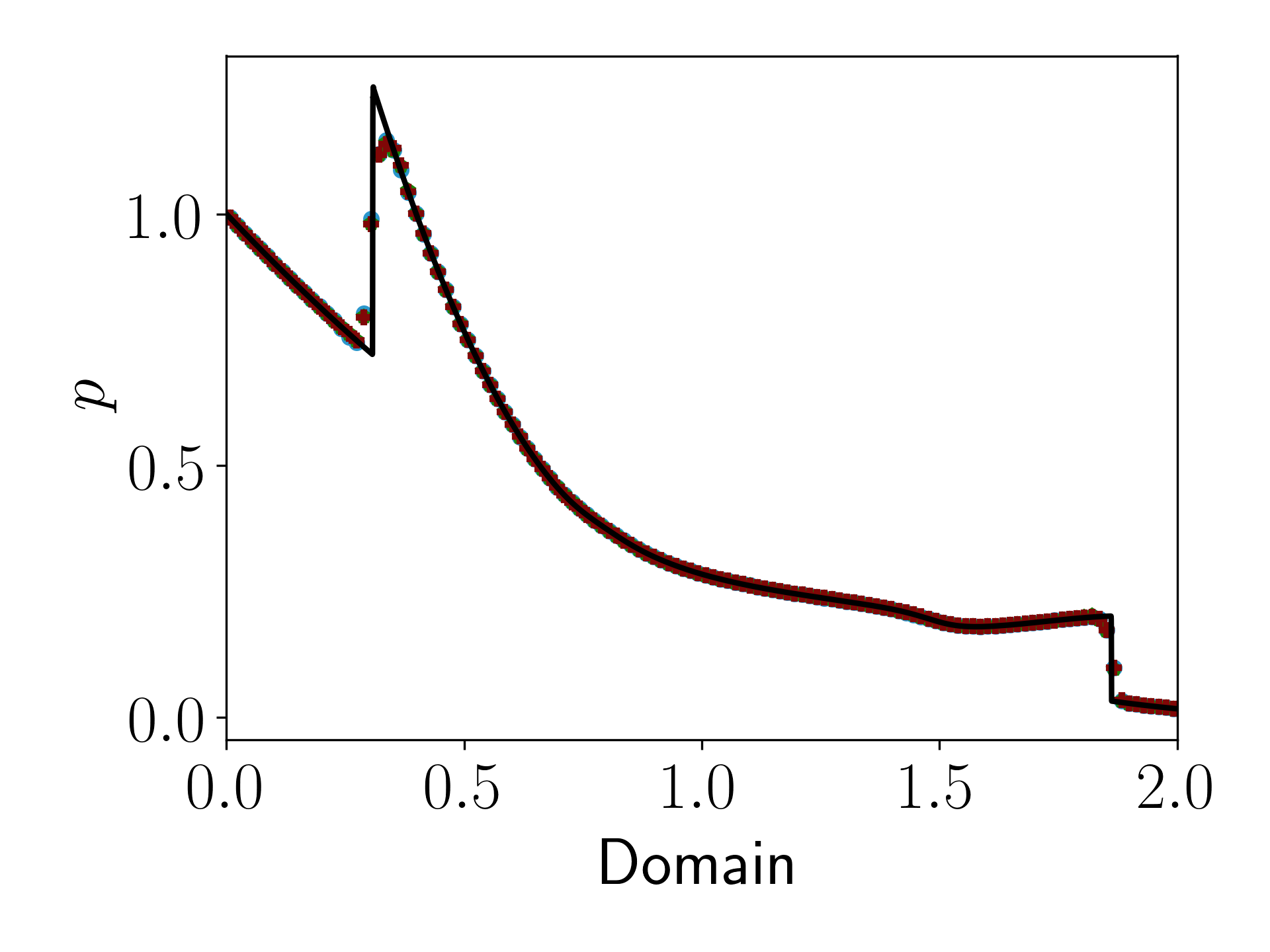
Figure 6: The left most column shows the convergence of the methods on the problem described in Section 3.1 with $A=1$. The upper part of the subplot shows the $L^{1}$-error of the pressure $p$. The lower subplot shows the convergence rate between two consecutive levels of refinement. The middle column shows the velocity $v$ and the right column shows the pressure $p$. The Mach number at the reference point is $M=$0.01$$. The scatter plots show the approximation with $N=128$ cells at the final time described in the text. The unbalanced, hydrostatically well-balanced and adiabatically well-balanced scheme is shown in blue, green and red, respectively. The solid black line is the reference solution.

3.2 One-dimensional, spherically symmetric experiments

The next two experiments are similar to the previous one, in the sense that we consider a stationary state both with and without a perturbation. However, this stationary state models the spherically symmetric, steady state accretion of gas onto a star known as Bondi accretion flows.

In a first numerical experiment the equilibrium solution is assumed to be continuous and either purely sub- or supersonic. In a second experiment we will consider an equilibrium in which the sub- and supersonic branches are joined by a stationary shock.

In both experiments the calculations are performed in spherical coordinates. The domain is $\Omega=[R_{0},R_{1}]$, $R_{0}=0.2$, $R_{1}=1.8$ and the gravitational potential is $\phi(r)=-Gm/r$ with $G=m=1$. The adiabatic index is $\gamma=4/3$. The ghost-cells are kept constant and equal to the initial conditions throughout the entire simulation. All numerical solvers in this subsection use the HLLC numerical flux and, unless stated explicitly otherwise, the monotonized centered limiter. The tolerance in Algorithm 1 is $tol=10^{-13}$. The CFL number is $c_{CFL}=0.45$.

3.2.1 Smooth equilibrium

The initial conditions are

$$\left(\rho^{0},v^{0},p^{0}\right)(r)=\left(\rho_{eq}(r),v_{eq}(r),p_{eq}(r)+A\exp(-(r-\bar{r})^{2}/\sigma^{2})\right)$$ (3.8)

with $\sigma=0.08$ and $\bar{r}=0.4R_{0}+0.6R_{1}$. The equilibrium is defined by the values of the density, velocity and speed of sound at the reference point $r_{0}=1$:

$$\rho_{0}=1,\quad c_{s,0}^{2}=\frac{1}{2},\quad v_{0}=-Mc_{s,0}.$$ (3.9)

This ensures that the critical point is located at $r_{0}=1$ which is the center of the domain. Therefore, we are sure that with $M=0.9$ the background of the initial conditions corresponds to the purely subsonic solution branch of Eq. 2.43 and for $M=2.0$ the background is purely supersonic. The parameter $A$ which controls the size of the perturbation will be specified later.

The initial conditions are computed by first extrapolating the equilibrium from the reference point $r_{0}$ to the cell-center of the cell just below $r_{0}$ and then iteratively downwards from one cell to the next. The analogous is done for the upper half of the domain. This improves the initial guess of the equilibrium extrapolation.

The convergence studies presented in this subsection are all run with $N=32,\dots,$2048$$ cells for both the unbalanced and adiabatically well-balanced method. The approximate solution computed by the adiabatically well-balanced scheme on $N=$8192$$ cells is used as a reference solution.

Well-balanced property

First we again check that the adiabatically well-balanced scheme is indeed well-balanced. Therefore, we choose $A=0$ and simulate until $t_{f}=4$ which corresponds to approximately four sound crossing times.

The results are shown in Table 10. The adiabatically well-balanced scheme preserves the discrete equilibrium up to machine precision. The unbalanced solver however accrues large $L^{1}$-errors for both values of the Mach number.

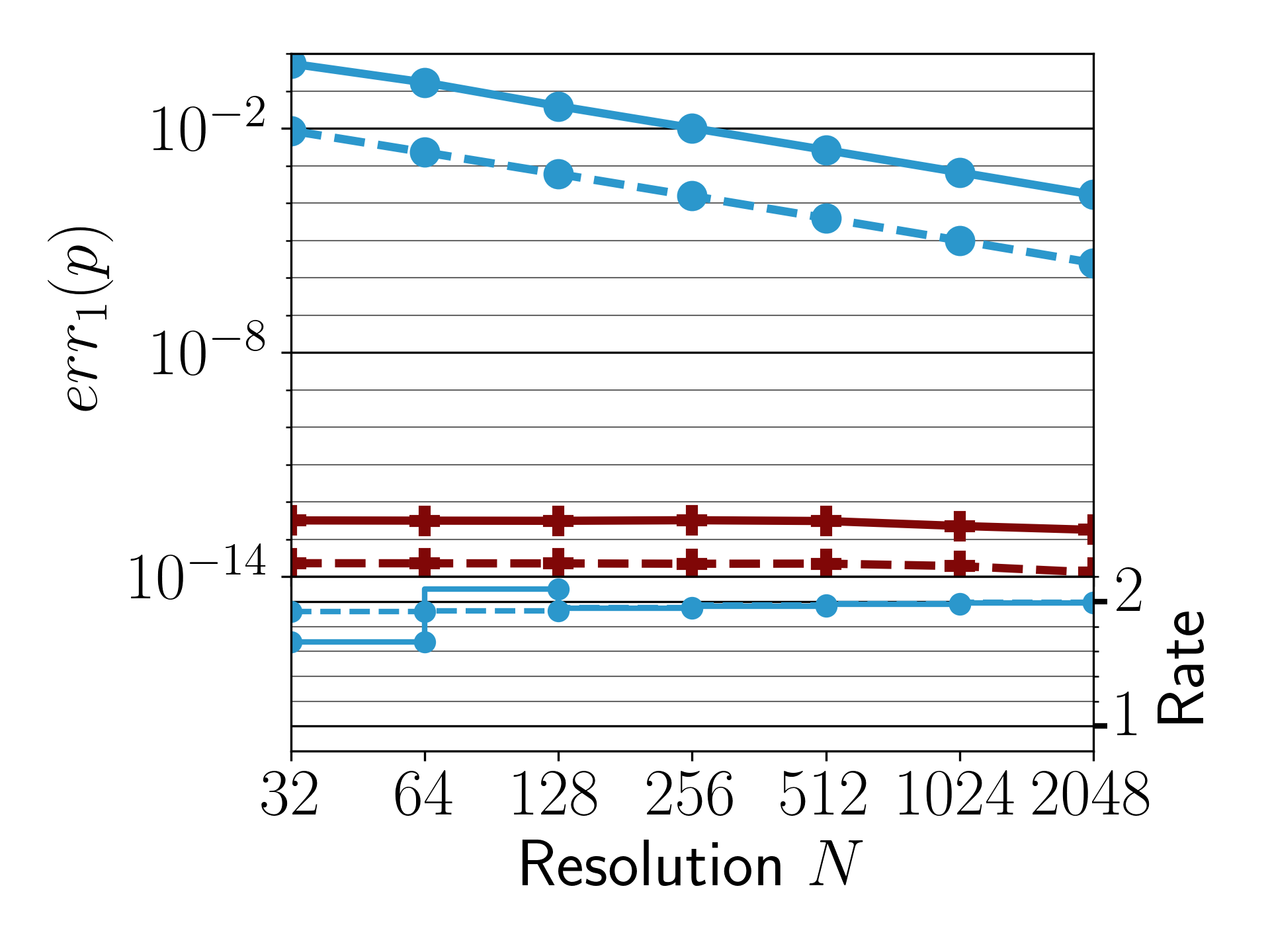
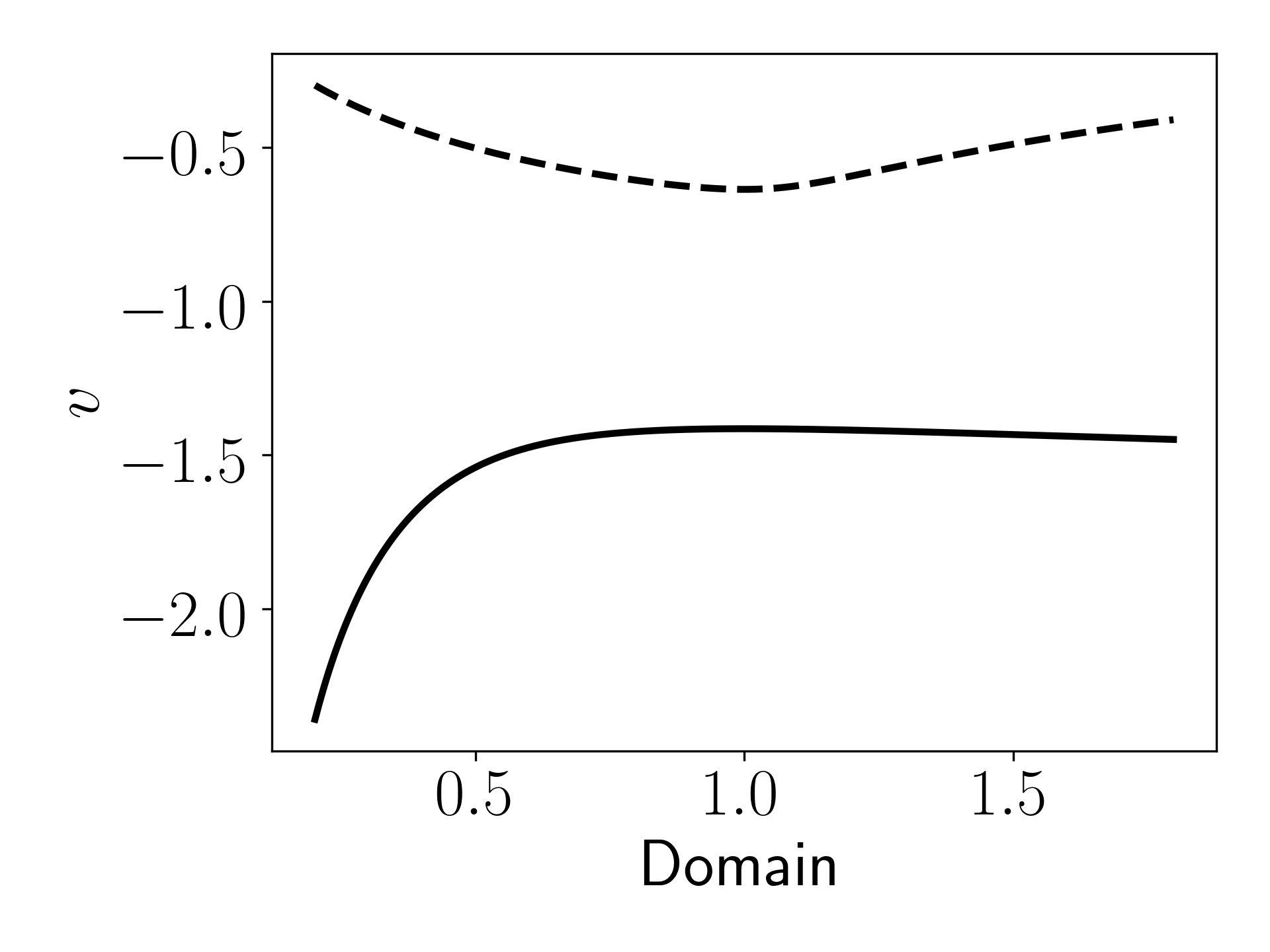
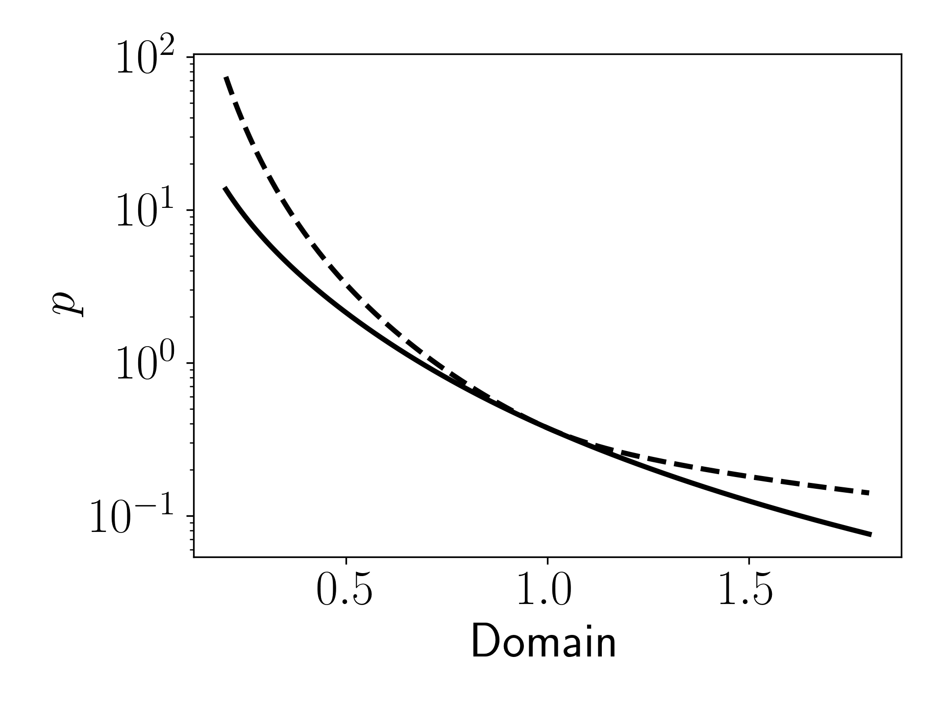
Figure 7: The left most column shows the well-balanced property of the methods on the problem described in Section 3.2.1 (with $A=0$). The upper part of the subplot shows the $L^{1}$-error of the pressure perturbation $\delta p$. The lower subplot shows the convergence rate between two consecutive levels of refinement. The unbalanced and adiabatically well-balanced scheme is shown in blue and red, respectively. The solid black line is the reference solution. The middle column shows the velocity and the right column shows the pressure. Solid lines represent $M=0.9$, the case $M=2.0$ is depicted as a dashed line.

Smooth wave propagation

We shall now consider a small perturbation $A=10^{-4}$ which remains smooth throughout the simulation. The final time is chosen to be

$$t_{f}=0.5\min\left(0.6\frac{R_{1}-R_{0}}{c_{0}+\lvert v_{0}\rvert},0.3\frac{R_{1}-R_{0}}{\max(c_{0}-\lvert v_{0}\rvert,10^{-10})}\right).$$ (3.10)

The results are show in Figs. 8 and 9 and the corresponding convergence table is Table 11. For both values of the Mach number the adiabatically well-balanced scheme resolves the wave faithfully, and does not perturb the regions of the domain which have not yet been reached by the wave. The resulting $L^{1}$-errors of the pressure perturbation are a factor of $10^{3}$ and $10^{2}$ smaller than those of the unbalanced method for $M=0.9$ and $M=2.0$ respectively. This dramatic improvement implies that the error on the lowest resolutions $N=32,64$ in the adiabatically well-balanced method is smaller than the errors of the standard scheme on $N=2048$ cells for $M=0.9$ and is comparable to the error on $N=512,1024$ cell for $M=2.0$.

Discontinuous wave propagation

Next we consider a large perturbation $A=100$. Due to the large amplitude of the wave we use the classical MinMod. The solution develops a discontinuity before the end of the simulation which is

$$t_{f}=0.08\min\left(0.6\frac{R_{1}-R_{0}}{c_{0}+\lvert v_{0}\rvert},0.3\frac{R_{1}-R_{0}}{\max(c_{0}-\lvert v_{0}\rvert,10^{-10})}\right).$$ (3.11)

The result is shown in Fig. 10 and the corresponding convergence table is Table 12. The adiabatically well-balanced scheme is robust in the presence of discontinuities and its performance is virtually indistinguishable from the unbalanced scheme.

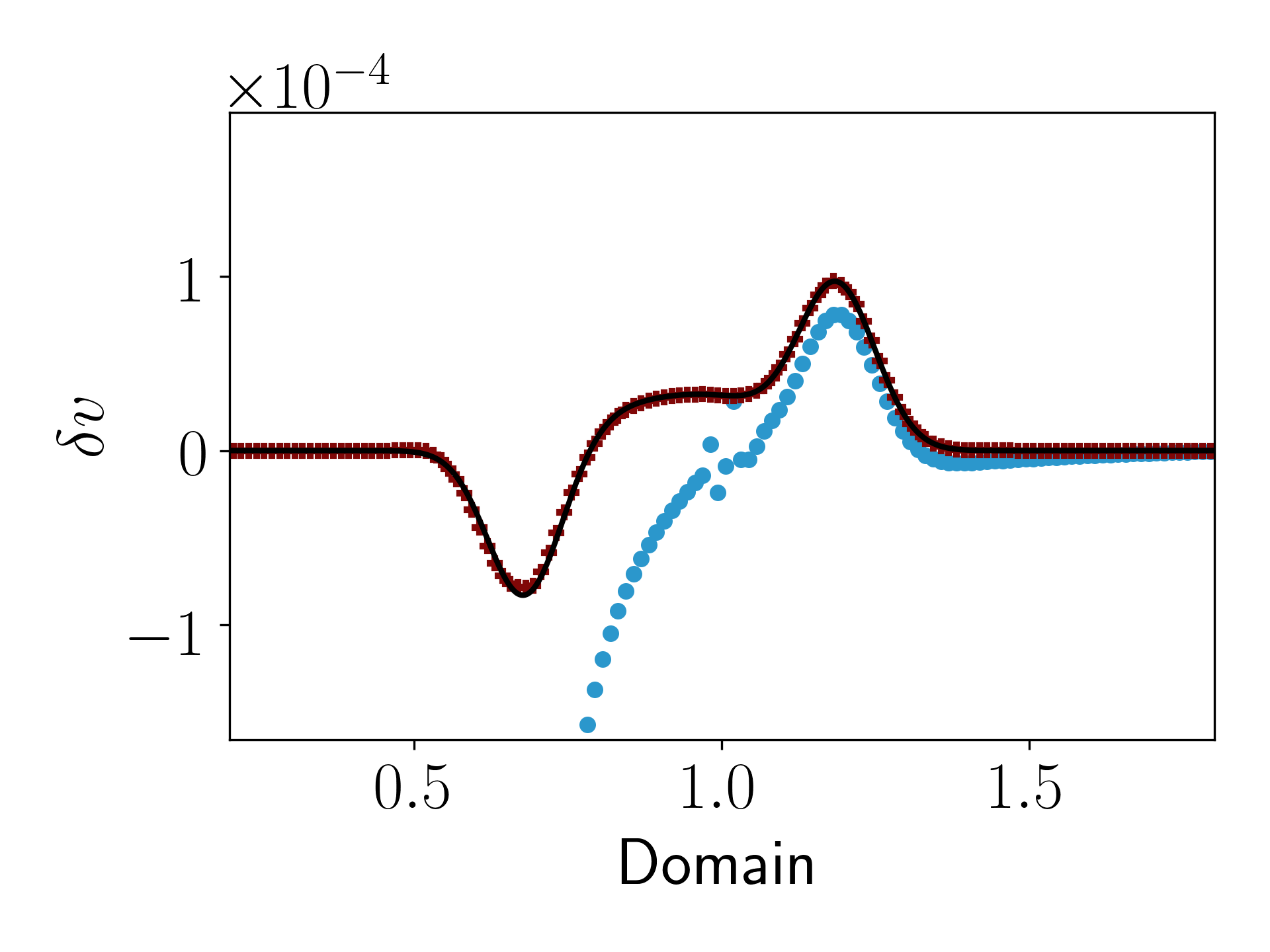
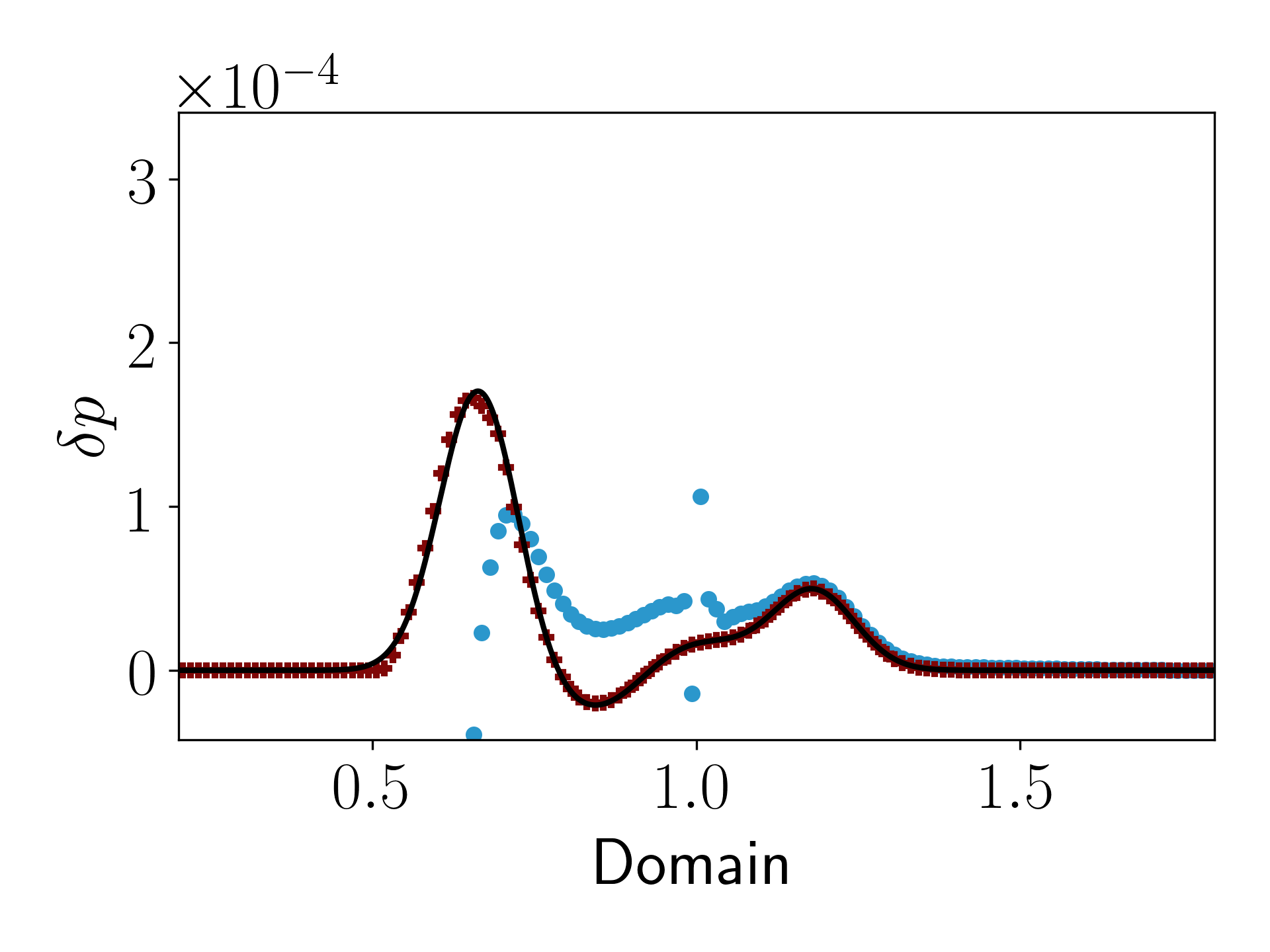
Figure 8: The left most column shows the convergence of the methods on the problem described in Section 3.2.1 with $A=10^{-4}$. The upper part of the subplot shows the $L^{1}$-error of the pressure perturbation $\delta p$. The lower subplot shows the convergence rate between two consecutive levels of refinement. The middle column shows the velocity perturbation $\delta v$ and the right column shows the pressure perturbation $\delta p$. The Mach number at the reference point is $M=0.9$. The scatter plots show the approximation with $N=128$ cells at the final time described in the text. The unbalanced and adiabatically well-balanced scheme is shown in blue and red, respectively. The solid black line is the reference solution.

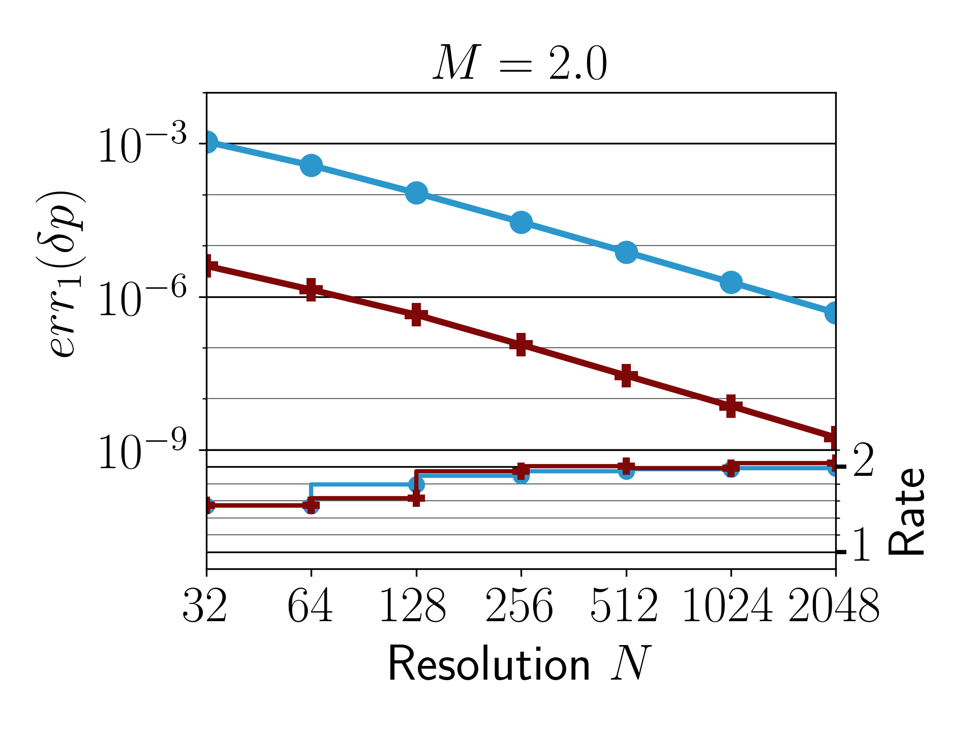
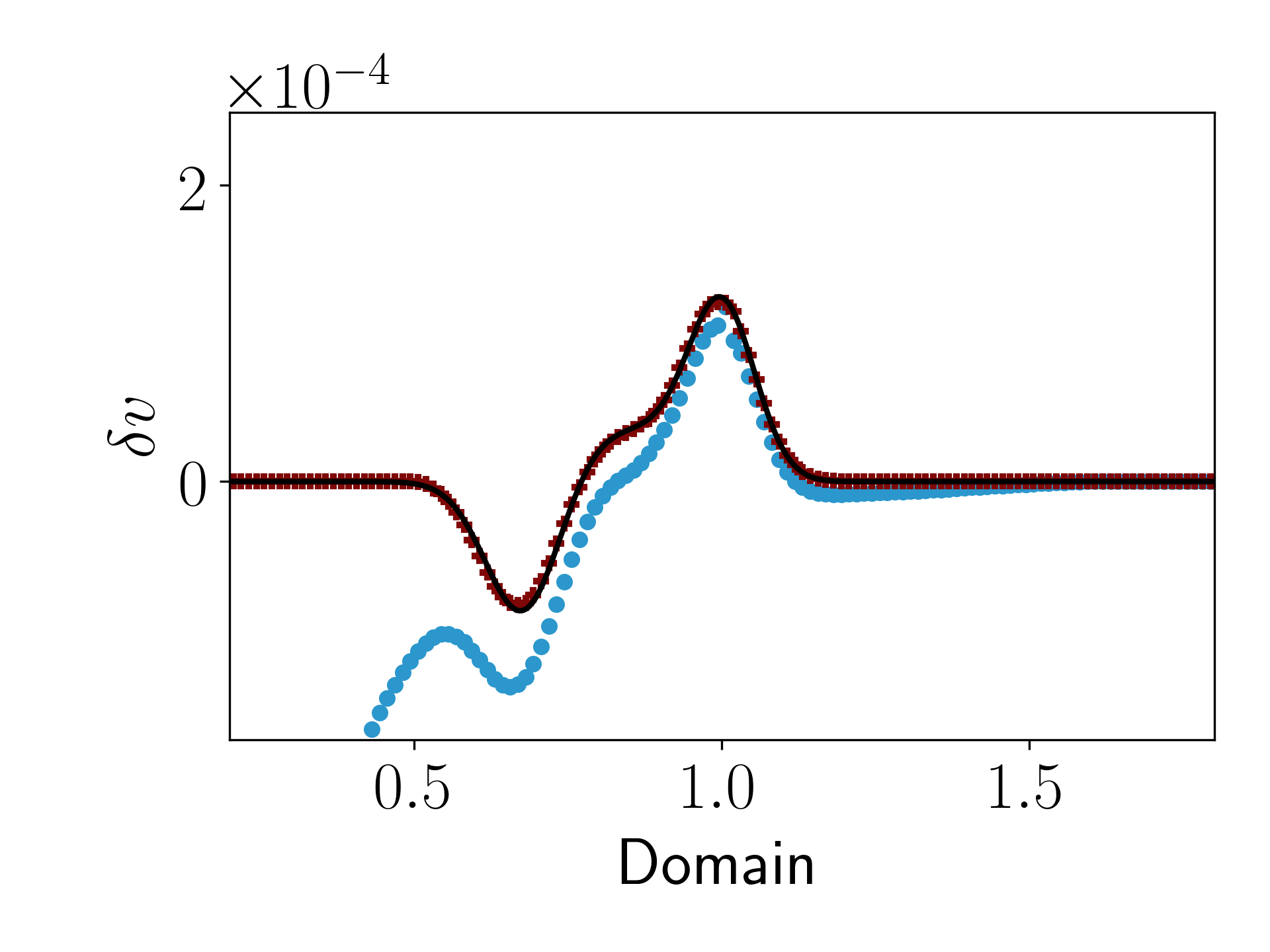
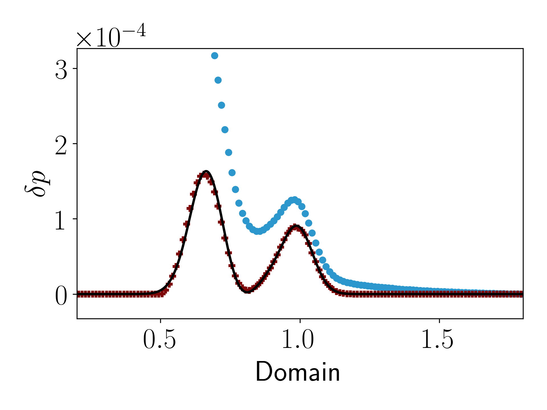
Figure 9: The figure shows the results for Section 3.2.1 with $A=10^{-4}$ and $M=2$. Please refer to the caption of Fig. 8 for a detailed caption.

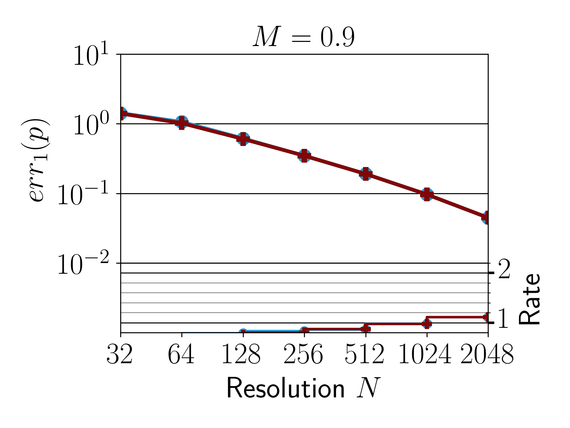
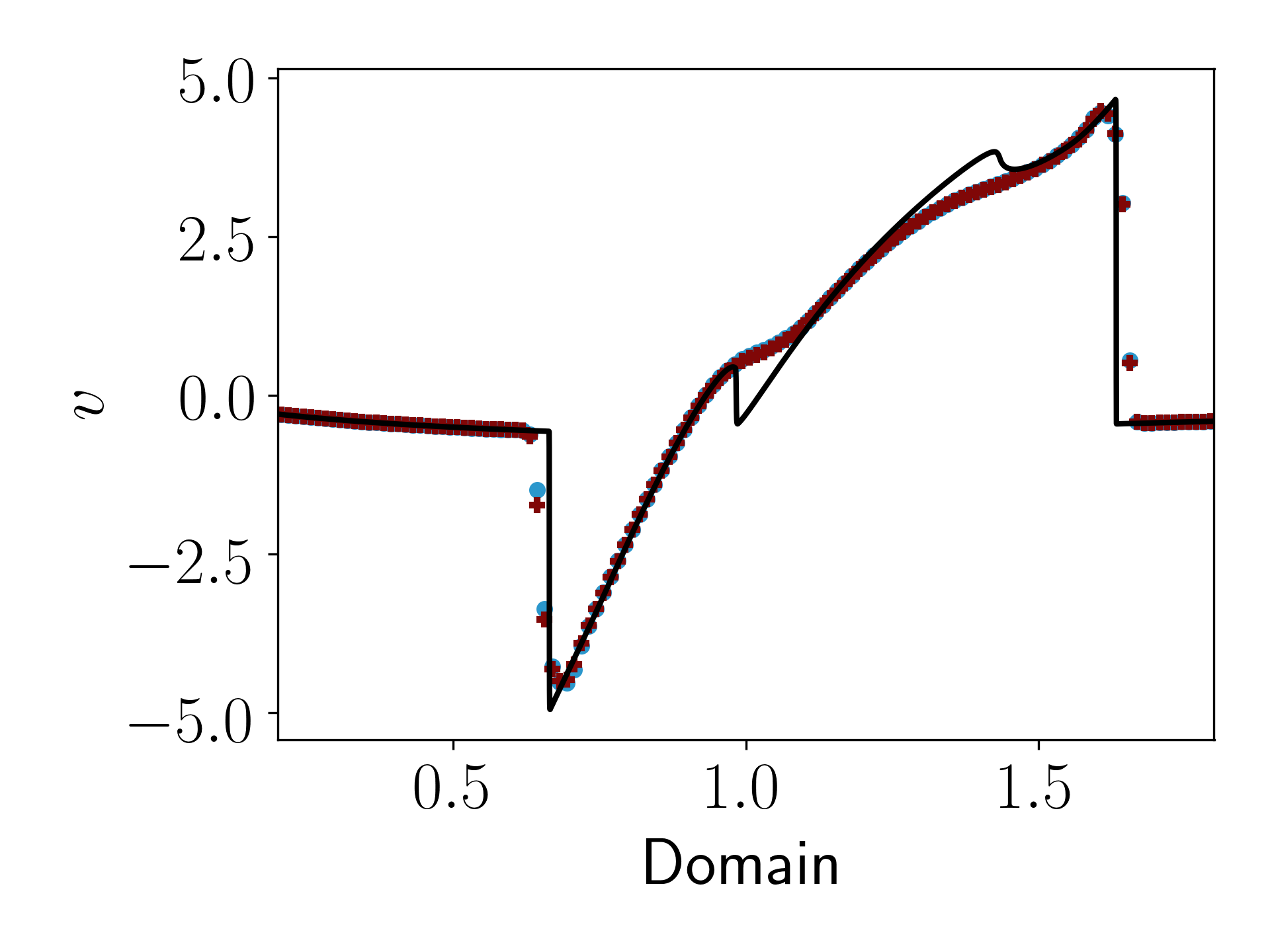
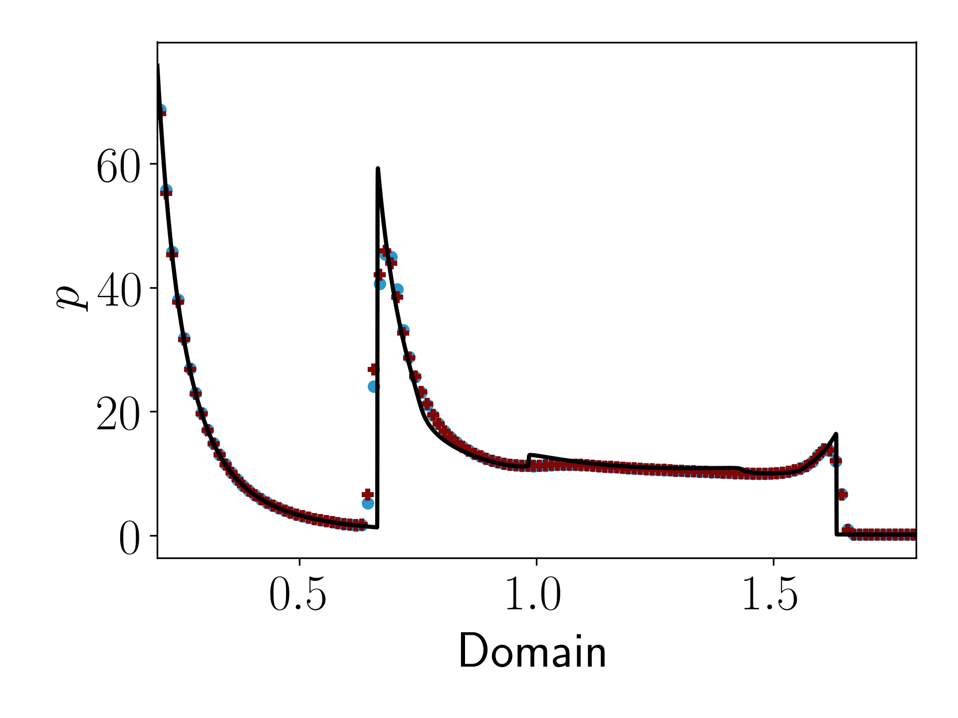
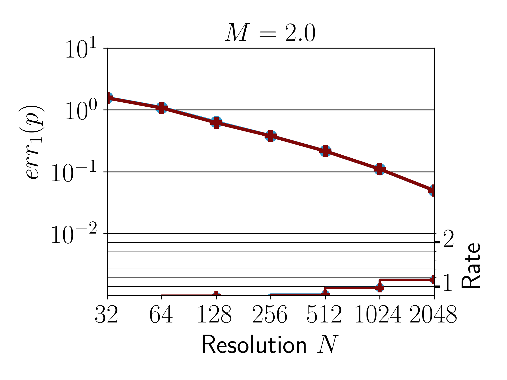
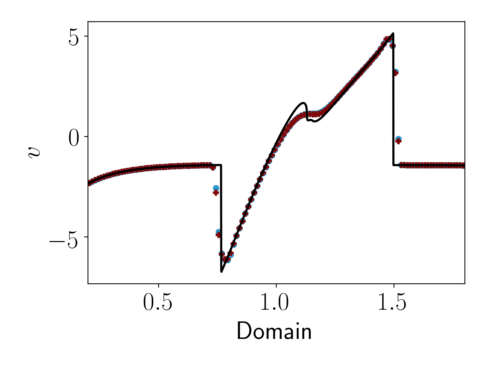
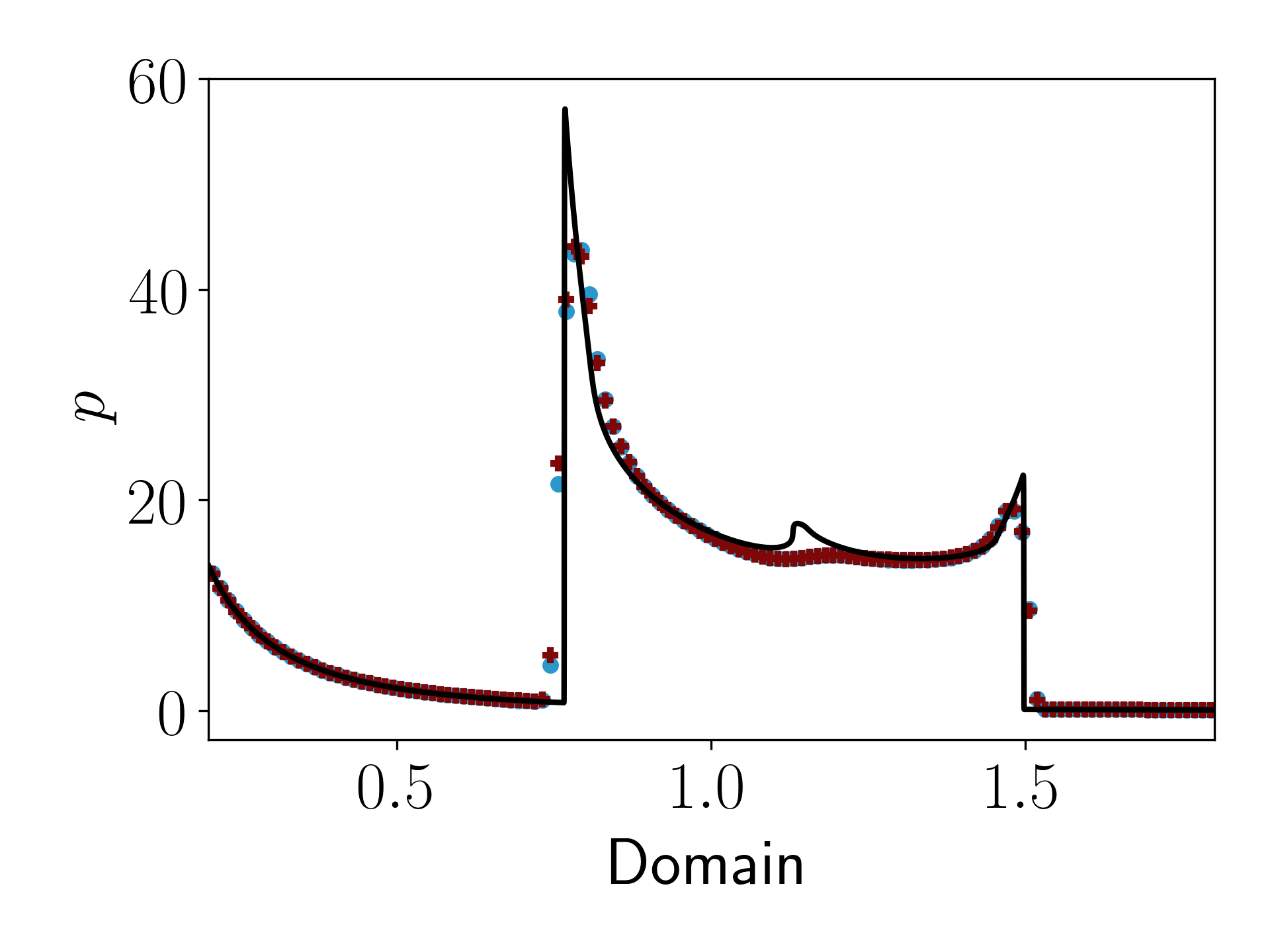
Figure 10: The left most column shows the convergence of the methods for the numerical experiment described in Section 3.2.1 with $A=100$. The upper part of the subplot shows the $L^{1}$-error of the pressure $p$. The lower subplot shows the convergence rate between two consecutive levels of refinement. The middle column shows the velocity $v$ and the right column shows the pressure $p$. The Mach number at the reference point is $M=$0.9$$. The scatter plots show the approximation with $N=128$ cells at the final time described in the text. The unbalanced and adiabatically well-balanced schemes are shown in blue and red, respectively. The solid black line is the reference solution.

3.2.2 Discontinuous equilibrium

So far, the equilibrium was either subsonic everywhere or supersonic everywhere, but never supersonic on one part of the domain and subsonic in another. In this experiment we will study a flow which is supersonic in the upper half and subsonic in the lower half of the domain. The two regions are joined by a stationary shock. In this experiment we use the classical MinMod rather than the monotonized centered limiter with the additional clipping of the pressure and density. Furthermore, we employ the HLL(E) flux which is able to resolve stationary discontinuities.

The shock is located at $r_{0}=1$. The pre-shock values are defined by

$$\rho_{0,1}=1,\quad c^{2}_{0,1}=\frac{1}{2},\quad v_{0,1}=-Mc_{0,1}$$ (3.12)

where $M=1.2$ is the pre-shock Mach number. The conditions immediately below the shock (e.g. post-shock) are given by the Rankine-Hugoniot conditions for a stationary shock [1]

$$\rho_{0,2}=\rho_{0,1}\frac{(\gamma+1)M^{2}}{(\gamma-1)M^{2}+2},\qquad p_{0,2}=p_{0,1}\left(\frac{2\gamma M^{2}}{\gamma+1}-\frac{\gamma-1}{\gamma+1}\right),\qquad v_{0,2}=\frac{\rho_{0,1}}{\rho_{0,2}}v_{0,1}.$$ (3.13)

The initial conditions in the upper ($k=1$) and lower ($k=2$) halves are computed by

$$\left(\rho^{0},v^{0},p^{0}\right)(r)=\left(\rho_{eq,k}(r),\ v_{eq,k}(r),\ p_{eq,k}(r)\right)$$ (3.14)

where $\boldsymbol{w}_{eq,k}$ is defined by the values $\rho_{0,k}$, $v_{0,k}$ and $c_{0,k}$ in $r_{0}=1$. Therefore, the initial condition consists of joining two, perturbed, equilibrium solutions by a stationary shock. Note that the initial conditions in the upper half of the domain are the same as in Section 3.2.1. Furthermore, the jump is chosen to lie exactly in the middle of the domain, hence if the number of cells is even, the shock is guaranteed to be located at the boundary between two cells. The final time is $t_{f}=2.0$ which corresponds to approximately two characteristic crossing times.

The adiabatically well-balanced scheme preserves this discontinuous equilibrium to machine precision, whereas the standard scheme accrues large errors. The results for $N=128$ is shown in Fig. 11.

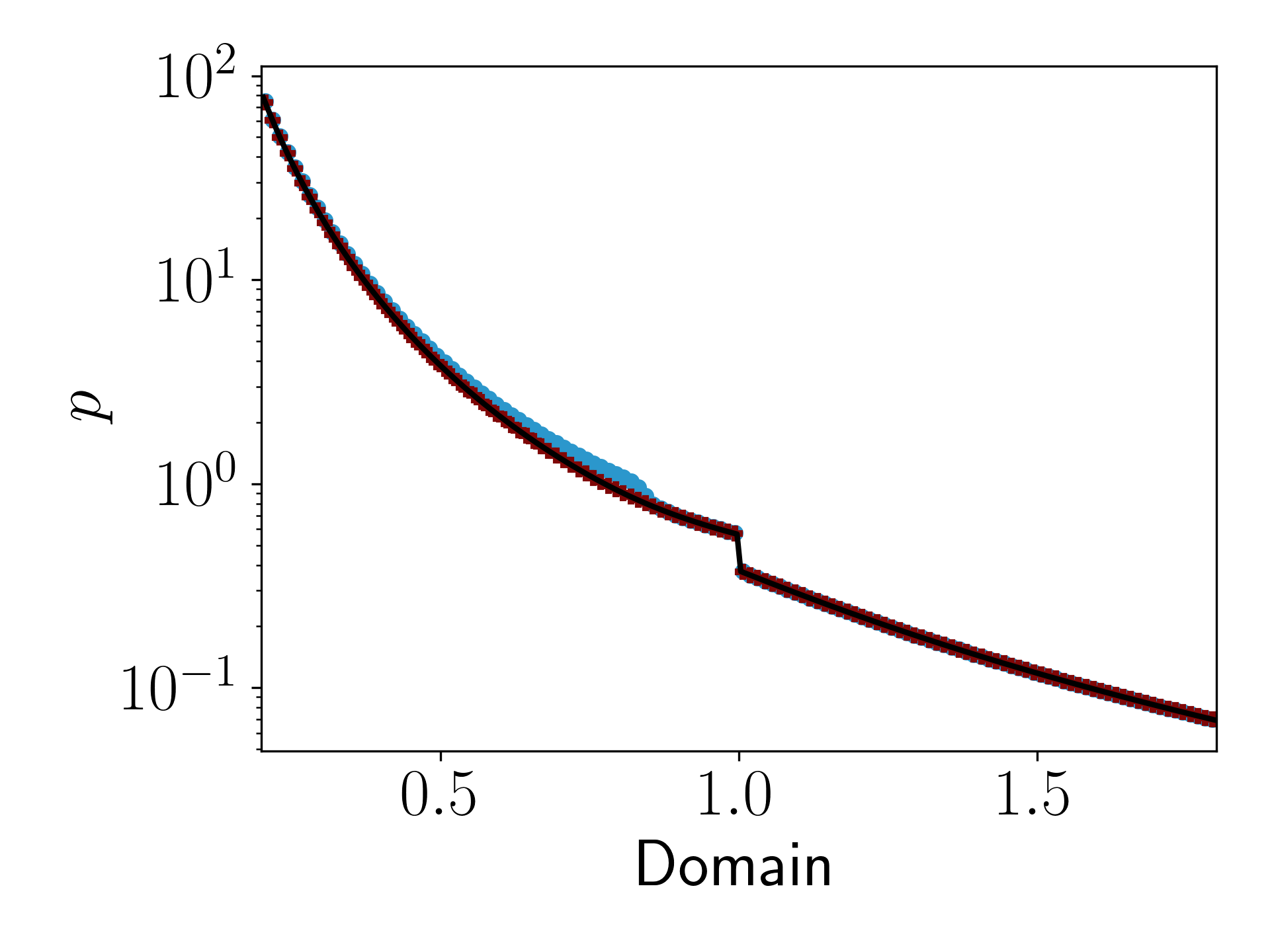
Figure 11: In the top row the density, velocity and pressure (left to right) of Section 3.2.2. The bottom row shows the error of those variables in the same order. All plots show an approximation of the solution with $N=128$ cells after two characteristic timescales. The unbalanced and adiabatically well-balanced scheme is shown in blue and red, respectively.

3.3 Stellar accretion

As a final test, we present the performance of our well-balanced schemes involving a complex multi-physics EoS. The test consists of the simulation of an astrophysical accretion scenario. In particular, we consider the accretion onto a compact object as it is typically encountered in a core-collapse. Such an event marks the death of a massive star and its transition to a compact object such as a neutron star or a black hole [65, 66, 67]. In a core-collapse supernova, a standing accretion shock arises as an expanding shock wave, generated by the sudden halt of the collapse of the core due to the stiffening of the EoS above super-nuclear density, stalls and remains nearly stationary for an extended period of time. During this period, the shock is revived by some (yet unknown in detail) combination of factors including neutrino heating, convection, rotation, and magnetic fields, triggering a formidable explosion. The standing accretion shock is subject to a dynamical instability commonly known as the standing accretion shock instability (SASI) [68]. The latter may have deep implications on the explosion mechanism itself, ejecta morphology, and pulsar kicks and spins (see e.g. Foglizzo et al. [69] and references therein).

A typical radial profile is shown in Fig. 12 (dashed lines). The radial profile was obtained from a simulation as described by Perego et al. [70]. The figure shows the standing accretion shock. Above the shock, matter is falling in supersonically. Below the shock, matter is falling in subsonically and pilling up onto the nascent proto-neutron star. We consider a highly simplified setup similar to [71, 72], which studies the dynamics of a standing accretion shock around a proto-neutron star restricted to the equatorial plane using cylindrical coordinates.

The computational domain spans $r\in[50,450]$ km in radius and the full angular realm $\varphi\in[0,2\pi]$. The accreting matter is modeled by a mixture of (photon) radiation, nuclei, electrons and positrons as provided by the publicly available Helmholtz EoS of Timmes and Swesty [73]. The gravitational attraction of the proto-neutron star is modeled by a point mass

$$\phi(r)=-\frac{GM}{r},$$ (3.15)

where $G$ is the gravitational constant and we set $M=1.3M_{\odot}$ (solar masses). We set the shock radius to $r_{\mathrm{sh}}=150$ km and the pre-shock conditions as

$$\rho_{\mathrm{pre}} =\phantom{-}2.0872995\times 10^{8}\leavevmode\nobreak\ \mathrm{g/cm}^{3},$$ (3.16)

$$v_{r,\mathrm{pre}} =-4.5618302\times 10^{4}\leavevmode\nobreak\ \mathrm{km/s},$$

$$v_{\varphi,\mathrm{pre}} =\phantom{-}0\leavevmode\nobreak\ \mathrm{km/s},$$

$$p_{\mathrm{pre}} =\phantom{-}1.1538646\times 10^{26}\leavevmode\nobreak\ \mathrm{erg/cm}^{3}.$$

The post-shock conditions are obtained from the Rankine-Hugoniot relations as

$$\rho_{\mathrm{post}} =\phantom{-}1.1989635\times 10^{9}\leavevmode\nobreak\ \mathrm{g/cm}^{3},$$ (3.17)

$$v_{r,\mathrm{post}} =-7.9417814\times 10^{3}\leavevmode\nobreak\ \mathrm{km/s},$$

$$v_{\varphi,\mathrm{pre}} =\phantom{-}0\leavevmode\nobreak\ \mathrm{km/s},$$

$$p_{\mathrm{post}} =\phantom{-}3.7029093\times 10^{27}\leavevmode\nobreak\ \mathrm{erg/cm}^{3}.$$

In the whole domain, we assume the matter to be composed of nickel isotope ⁵⁶Ni. By numerically solving for the steady state conditions, one obtains the solid line profiles in Fig. 12. As apparent from the figure, the simplified setup matches the more complex model quite well (despite the different EoS and geometry).

Next, we give some implementation details related to the complex multi-physics EoS. In the publicly available Helmholtz EoS, the photons are treated as black body radiation in local thermal equilibrium and the nuclei by an ideal gas law. The electrons and positrons are treated in a tabular manner allowing speeds arbitrarily close to the causal limits and arbitrary degree of degeneracy with a thermodynamically consistent interpolation method. The EoS interface provides all the relevant thermodynamic quantities given the temperature $T$, density $\rho$ and composition. The composition is specified by the triplet $(X_{i},A_{i},Z_{i})$ for each isotope $i$, where $X_{i}$ is the mass fraction, $A_{i}$ the mass number and $Z_{i}$ the atomic number. In the present problem setup, we thus have only one isotope with $(X_{1}=1,A_{1}=56,Z_{1}=28)$. Because we evolve the Euler equations in conservative form, we have to determine the temperature corresponding to a given density $\rho$ and specific internal energy $e$. Similarly in the local equilibrium reconstruction, we have to determine the temperature $T$ and the density $\rho$ corresponding to a given specific enthalpy $h$ and entropy $s$. This is implemented with robust root finding algorithms combining Newton’s method for speed and the bisection method for robustness (see e.g. Press et al.[74] for details.).

In the following, we show the performance of the second-order adiabatically well-balanced scheme and compare it to a standard second-order unbalanced scheme. Both schemes have been modified in a standard and identical fashion to cope with the cylindrical geometry. The standard unbalanced scheme is obtained by simply disabling the well-balanced reconstruction and source term discretization of the well-balanced scheme. Both schemes use the HLL Riemann solver with simple wave speed estimates from the fastest left/right traveling characteristic speeds at the cell interface (see e.g. Toro [48]). Note that these speed estimates will not exactly resolve isolated shocks. Therefore, we divide the full test problem in a subsonic $r\in[50,150]$ km and a supersonic $r\in[150,450]$ part when studying the schemes’ well-balanced property in Section 3.3.1 and the wave propagation properties in Section 3.3.2. In Section 3.3.3, we show the performance of the schemes on the full problem. In all the tests, the computational domain spans the full angular realm $\varphi\in[0,2\pi]$.

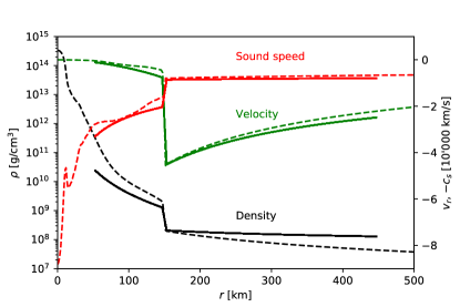
Figure 12: Radial profiles of density (black lines), radial velocity (green lines) and sound speed (red lines) for the stellar accretion test problem Section 3.3. The dashed lines show the profiles from a core-collapse simulation as described by Perego et al. [70]. The solid lines show the highly simplified setup considered in the stellar accretion test problem.

3.3.1 Well-balanced property

We begin by numerically verifying the well-balancing properties of the developed scheme. For this purpose, we evolve the subsonic and supersonic accretion steady states for two characteristic times $t_{f}=2\tau_{\mathrm{char}}$, and several resolutions in radial and angular directions: $(N_{r},N_{\varphi})=(32,64)$, $(64,128)$, $(128,256)$, $(256,512)$. The domain boundaries in radial direction are simply kept frozen in time at the equilibrium state. The relative equilibrium errors in density, radial velocity and pressure are displayed in Table 1 for the subsonic and Table 2 for the supersonic parts. We observe that the well-balanced scheme produces errors on the order of the precision with which the local equilibrium is numerically solved ($tol=10^{-13}$). In contrast, the unbalanced scheme suffers from comparatively large errors and is unable to maintain the steady state.

$(N_{r},N_{\varphi})$	$relerr_{1}(\rho)$	$relerr_{1}(v_{r})$	$relerr_{1}(p)$
( 32, 64)	2.33E-02 / 4.13E-13	1.80E-01 / 9.95E-13	2.59E-02 / 4.07E-13
( 64, 128)	4.14E-03 / 7.45E-13	3.61E-02 / 1.27E-11	4.46E-03 / 6.32E-13
(128, 256)	7.81E-04 / 2.17E-12	8.89E-03 / 4.99E-11	8.37E-04 / 2.02E-12
(256, 512)	1.86E-04 / 5.85E-12	1.74E-03 / 9.09E-11	1.91E-04 / 5.31E-12
Order	2.33 / -	2.21 / -	2.37 / -

Table 1: Relative equilibrium error in density, radial velocity and pressure for the subsonic accretion steady state computed with the un-/well-balanced second-order schemes for two characteristic times $t_{f}=2\tau_{\mathrm{char}}\approx 6.872778\times 10^{-3}$ s.

$(N_{r},N_{\varphi})$	$relerr_{1}(\rho)$	$relerr_{1}(v_{r})$	$relerr_{1}(p)$
( 32, 64)	1.58E-04 / 2.68E-15	3.36E-04 / 2.94E-15	2.13E-04 / 1.22E-14
( 64, 128)	3.78E-05 / 1.87E-15	8.42E-05 / 1.32E-15	4.81E-05 / 9.95E-15
(128, 256)	9.24E-06 / 1.25E-12	2.11E-05 / 1.25E-12	1.13E-05 / 8.15E-12
(256, 512)	2.28E-06 / 8.30E-13	5.29E-06 / 8.39E-13	2.75E-06 / 5.84E-12
Order	2.04 / -	2.00 / -	2.09 / -

Table 2: Relative equilibrium error in density, radial velocity and pressure for the supersonic accretion steady state computed with the un-/well-balanced second-order schemes for two characteristic times $t_{f}=2\tau_{\mathrm{char}}\approx 1.506179\times 10^{-2}$ s.

3.3.2 Small and large amplitude perturbations

To verify the capability of the schemes to evolve perturbation on top of the steady state, we add five Gaussian hump density perturbations to the flow as

$$\rho(r,\varphi)=\left(1+A\sum_{k=0}^{4}e^{-\frac{x_{k}^{2}+y_{k}^{2}}{w^{2}}}\right)\rho_{eq}(r)$$ (3.18)

with

$$x_{k} =r\cos(\varphi)-r_{0}\cos(\varphi_{k}),$$ (3.19)

$$y_{k} =r\sin(\varphi)-r_{0}\sin(\varphi_{k})$$

and $\varphi_{k}=2\pi k/5$ for $k=0,\dots,4$. Here, $\rho_{eq}(r)$ is the subsonic and supersonic steady state, respectively, and $r_{0}$ is the radius, $w$ the width and $A$ the amplitude of the perturbations. The boundary conditions are kept frozen at the initial steady state.

For the subsonic case, we set $r_{0}=110$ km and $w=10$ km. The final time is $t_{f}=1.247314\times 10^{-3}\leavevmode\nobreak\ \mathrm{s}\leavevmode\nobreak\ \approx 0.36\leavevmode\nobreak\ \tau_{\mathrm{char}}$. The small amplitude test is run with $A=10^{-3}$ and the relative perturbation errors are displayed in Table 3. The errors of the well-balanced scheme are consistently smaller by 2-3 orders of magnitude than errors of the unbalanced scheme. It is clear that the well-balanced scheme is vastly superior in resolving the small perturbations. Furthermore, we observe that the errors of the well-balanced scheme at the lowest resolution are comparable to the errors of the unbalanced scheme at the highest resolution. This is further illustrated in the left panel of Fig. 13 from which it is apparent that the unbalanced scheme suffers from large spurious deviations. Both schemes attain their design second-order accuracy.

For the supersonic case, we use the parameters $r_{0}=375$ km and $w=20$ km. The final time is $t_{f}=4.518538\times 10^{-3}\leavevmode\nobreak\ \mathrm{s}\leavevmode\nobreak\ \approx 0.30\leavevmode\nobreak\ \tau_{\mathrm{char}}$. The small amplitude test is run with $A=10^{-3}$ and the relative perturbation errors are displayed in Table 5. Like in the previous case, we observe that the errors of the well-balanced scheme are consistently smaller by several orders of magnitude. This is further highlighted in the right panel of Fig. 13 from which it is apparent that the unbalanced scheme suffers from large spurious differences.

To assess the robustness of the schemes, we run both the subsonic and the supersonic test case with a hundred times greater perturbation $A=10^{-1}$. The final times are identical to the respective small amplitude experiments. The results are shown in Table 4 for the subsonic case and in Table 6. As to be expected, the difference between the well-balanced and unbalanced schemes decreases as the size of the perturbation is increased. Therefore, we observe that there is no loss in robustness and resolution capability for large amplitude perturbations with the well-balanced scheme compared to the unbalanced one.

$(N_{r},N_{\varphi})$	$relerr_{1}(\delta\rho)$	$relerr_{1}(\delta v_{r})$	$relerr_{1}(\delta p)$
( 32, 64)	6.01E-03 / 6.22E-06	4.65E-02 / 5.66E-05	8.63E-03 / 1.39E-06
( 64, 128)	1.27E-03 / 2.59E-06	9.97E-03 / 2.46E-05	1.66E-03 / 4.66E-07
(128, 256)	2.85E-04 / 7.66E-07	2.31E-03 / 6.93E-06	3.64E-04 / 1.19E-07
(256, 512)	6.71E-05 / 1.23E-07	5.57E-04 / 1.13E-06	8.50E-05 / 2.28E-08
Order	2.16 / 1.87	2.13 / 1.88	2.22 / 1.98

Table 3: Relative perturbation error in density, radial velocity and pressure for the subsonic accretion equilibrium with small amplitude density perturbations computed with the un-/well-balanced second-order schemes.

$(N_{r},N_{\varphi})$	$relerr_{1}(\delta\rho)$	$relerr_{1}(\delta v_{r})$	$relerr_{1}(\delta p)$
( 32, 64)	6.26E-03 / 6.16E-04	4.87E-02 / 5.43E-03	8.63E-03 / 1.33E-04
( 64, 128)	1.44E-03 / 2.57E-04	1.14E-02 / 2.32E-03	1.67E-03 / 4.46E-05
(128, 256)	3.42E-04 / 7.61E-05	2.71E-03 / 6.42E-04	3.65E-04 / 1.11E-05
(256, 512)	7.52E-05 / 1.22E-05	6.10E-04 / 1.03E-04	8.51E-05 / 2.14E-06
Order	2.12 / 1.87	2.10 / 1.90	2.22 / 1.99

Table 4: Relative perturbation error in density, radial velocity and pressure for the subsonic accretion equilibrium with large amplitude density perturbations computed with the un-/well-balanced second-order schemes.

$(N_{r},N_{\varphi})$	$relerr_{1}(\delta\rho)$	$relerr_{1}(\delta v_{r})$	$relerr_{1}(\delta p)$
( 32, 64)	4.74E-05 / 7.84E-06	2.97E-04 / 8.41E-08	5.52E-05 / 2.14E-07
( 64, 128)	1.36E-05 / 4.82E-06	7.47E-05 / 5.27E-08	9.95E-06 / 7.63E-08
(128, 256)	3.75E-06 / 1.68E-06	1.88E-05 / 1.88E-08	2.06E-06 / 2.47E-08
(256, 512)	9.34E-07 / 4.36E-07	4.70E-06 / 4.79E-09	4.67E-07 / 6.47E-09
Order	2.12 / 1.40	1.99 / 1.39	2.29 / 1.68

Table 5: Relative perturbation error in density, radial velocity and pressure for the supersonic accretion equilibrium with small amplitude density perturbations computed with the un-/well-balanced second-order schemes.

$(N_{r},N_{\varphi})$	$relerr_{1}(\delta\rho)$	$relerr_{1}(\delta v_{r})$	$relerr_{1}(\delta p)$
( 32, 64)	8.49E-04 / 7.62E-04	2.98E-04 / 7.66E-06	6.36E-05 / 2.27E-05
( 64, 128)	4.89E-04 / 4.73E-04	7.64E-05 / 4.95E-06	1.47E-05 / 7.46E-06
(128, 256)	1.67E-04 / 1.65E-04	1.97E-05 / 1.74E-06	4.01E-06 / 2.33E-06
(256, 512)	4.30E-05 / 4.26E-05	4.87E-06 / 4.36E-07	9.62E-07 / 5.96E-07
Order	1.45 / 1.40	1.98 / 1.39	2.00 / 1.74

Table 6: Relative perturbation error in density, radial velocity and pressure for the supersonic accretion equilibrium with large amplitude density perturbations computed with the un-/well-balanced second-order schemes.

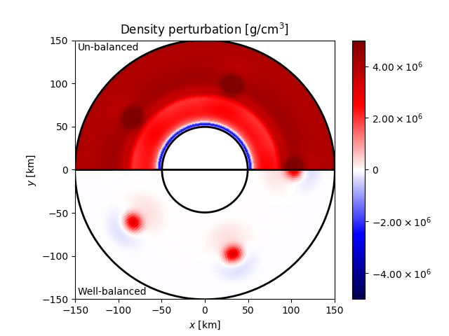
(a) Subsonic steady state

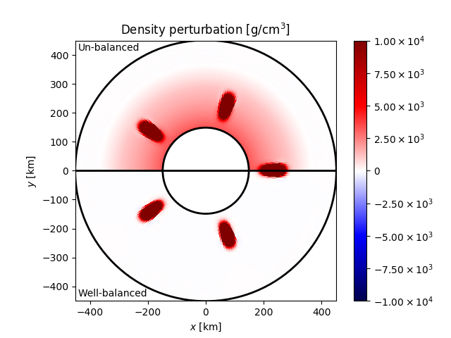
(b) Supersonic steady state

Figure 13: Small amplitude density perturbations on the subsonic (left panel) and supersonic (right panel) steady state. In both panels, the lower/upper plane show the results obtained with the un-/well-balanced schemes at resolution $(N_{r},N_{\varphi})=(128,256)$, respectively. The color axis is clipped to highlight the absence of spurious deviations away from the perturbations for the well-balanced scheme.

3.3.3 Full problem

As a final case, we test the ability of the schemes to preserve the full problem joining the sub- and super-sonic regions with a standing shock. We evolve the setup for several characteristic time scales $t_{f}=4\tau_{\mathrm{char}}$. The outer radial boundary is kept frozen at the initial state and we impose outflow conditions at the lower boundary. As noted previously, the HLL Riemann solver will not exactly resolve stationary shocks. Therefore, we can not expect the well-balanced scheme to exactly preserve the transonic steady state.

In the right panel of Fig. 14, we show the shock radius as a function of time for several resolutions $(N_{r},N_{\varphi})=(128,256),(256,512),(512,1024)$. The latter is simply evaluated by determining the radius of the maximum absolute difference in radial velocity. From the figure, it is apparent that the well-balanced scheme (blue lines) is able to preserve the initial shock position very well. On the other hand, the shock position deviates for the unbalanced schemes. This is further illustrated in the left panel of Fig. 14, where we display a contour of radial velocity of the initial condition together with the results obtained with the well-balanced and unbalanced schemes after two characteristic time scales. We observe that the results of the well-balanced scheme are virtually indistinguishable from the initial conditions.

However, we note that a thorough analysis of the standing accretion shock instability onset and dynamics is beyond the scope of the present paper.

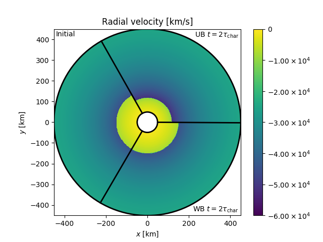
(a) Accretion shock

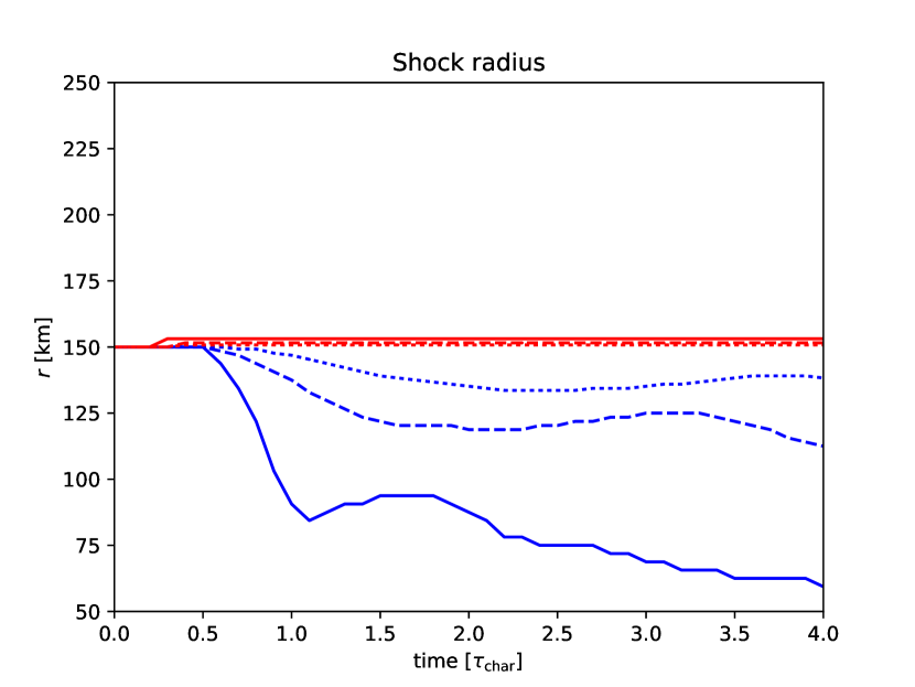
(b) Shock radius

Figure 14: The left panel shows the radial velocity contour for resolution $(N_{r},N_{\varphi})=(256,512)$. The right panel shows the shock radius as a function of time for un-/well-balanced (blue/red lines) for resolutions $(N_{r},N_{\varphi})=(128,256),(256,512),(512,1024)$ (solid, dashed, dotted lines).

4 Conclusion

In this paper, we have presented novel well-balanced first- and second-order accurate finite volume schemes for the Euler equations with gravity. The schemes are able to exactly (up to round-off errors) preserve any one-dimensional steady adiabatic flow. Flows of this type are an idealized model for accretion and wind phenomena commonly encountered in astrophysics. The method is based on a local equilibrium reconstruction combined with a well-balanced source term discretization. The schemes are extended to cylindrical and spherical geometries. A dimension-by-dimension extension to multiple dimensions is also proposed. However, the latter is only exactly well-balanced for multi-dimensional states with streamlines aligned along a computational axis. The schemes’ performance and robustness are verified on several numerical experiments. The last test case consists of a model stellar accretion setup commonly encountered in core-collapse supernovae scenarios and features a complex multi-physics equation of state.

The current paper deals with a large class of adiabatic steady states. However, there are scenarios where the flow does not proceed adiabatically, e.g. due to radiation losses. This is especially the case in astrophysics. Developing schemes capable of balancing such non-adiabatic steady states is indeed worthwhile. Moreover, the current schemes are limited to steady states with streamlines aligned with one computational axis. Although the usage of curvilinear coordinates may help to deal with this limitation, it would be computationally desirable to remove this restriction. For instance, cylindrical and spherical coordinates feature coordinate singularities which have implications for the resolution and regularity of the grid and, thereby, the size of time steps. An extension beyond second-order accuracy is also highly desirable. Such extensions are subject to current research and will be dealt with in forthcoming publications.

Appendix A Local equilibrium determination for general EoS

Evaluating the equilibrium $\boldsymbol{W}_{eq,i}$ in $x$ for a general convex EoS requires a slightly different algorithm than the one presented in the main text, i.e. Algorithm 1. The differences are mainly due to the fact that $\varepsilon_{\ast}$ and $\rho_{\ast}$ cannot be computed analytically. Therefore, instead of comparing $\rho^{(k)}$ with $\rho_{\ast}$ to determine if it switched from the sub- to the supersonic branch (or vice versa), we propose to look at the derivative of $\varepsilon$ instead. The algorithm terminates for four reasons: a) the equilibrium is found, b) the algorithm fails to make any progress towards a root, c) the algorithm has converged towards the minimum, or d) the maximum number of iterations is reached. In the latter three cases we consider the algorithm to have failed to find an equilibrium. Subsequently, that cell will be marked and the standard reconstruction and source term are used in that cell.

Initial guess $\rho^{(0)}=\rho_{0}$;

for k = 0, 1, 2, … do

      $\rho^{(trial)}=\rho^{(k)}-\operatorname{sign}(\frac{\varepsilon(\rho^{(k)})}{\varepsilon^{\prime}(\rho^{(k)})})\min(\lvert\frac{\varepsilon(\rho^{(k)})}{\varepsilon^{\prime}(\rho^{(k)})}\rvert,\rho^{(k)}/4)$;

     

     $\rho^{(trial)}=\max(0,\rho^{(trial)})$;

     

     for $\ell$ = 0, 1, 2, … do

           if $\varepsilon^{\prime}(\rho^{(0)})\leavevmode\nobreak\ \varepsilon^{\prime}(\rho^{(trial)})<0$ then

                $\rho^{(trial)}=\frac{1}{2}(\rho^{(trial)}+\rho^{(k)})$

                end if

               

                end for

               

               $\Delta\rho=\rho^{(trial)}-\rho^{(k)}$;

                $\rho^{(k+1)}=\rho^{(trial)}$;

               

               if $\lvert\varepsilon(\rho^{(k+1)})\rvert<tol\leavevmode\nobreak\ \lvert\varepsilon_{0}-\phi(x)\rvert$ then

                     Successfully found the equilibrium.

                     Stop

                     end if

                    

                    if $\lvert\Delta\rho\rvert<tol\leavevmode\nobreak\ \max(\rho^{(0)},\rho^{(k+1)})$ then

                          Failed due to lacking progress per step.

                          Stop

                          end if

                         

                         if $\lvert\varepsilon^{\prime}(\rho^{(k+1)})\rho^{(k+1)}\rvert<tol\leavevmode\nobreak\ \lvert\varepsilon(\rho^{(k+1)})\rvert$ then

                               Converged to minimum.

                               Stop

                               end if

                              

                               end for

Algorithm 2 Local equilibrium determination for a general convex EoS.

Appendix B Convergence tables

In this section we present the convergence tables for the numerical experiments presented in Section 3.

N	unbalanced		hydrostatic		full
$M=$0$$	$\operatorname{err}_{1}($$\delta p$$)$	Rate	$\operatorname{err}_{1}($$\delta p$$)$	Rate	$\operatorname{err}_{1}($$\delta p$$)$	Rate
32	$3.38\text{\times}{10}^{-05}$	–	$6.78\text{\times}{10}^{-15}$	–	$6.70\text{\times}{10}^{-15}$	–
64	$7.05\text{\times}{10}^{-06}$	2.26	$6.52\text{\times}{10}^{-15}$	0.06	$6.85\text{\times}{10}^{-15}$	-0.03
128	$1.60\text{\times}{10}^{-06}$	2.14	$6.65\text{\times}{10}^{-15}$	-0.03	$6.14\text{\times}{10}^{-15}$	0.16
256	$3.79\text{\times}{10}^{-07}$	2.07	$6.82\text{\times}{10}^{-15}$	-0.04	$6.80\text{\times}{10}^{-15}$	-0.15
512	$9.23\text{\times}{10}^{-08}$	2.04	$7.38\text{\times}{10}^{-15}$	-0.11	$7.06\text{\times}{10}^{-15}$	-0.05
1024	$2.28\text{\times}{10}^{-08}$	2.02	$7.04\text{\times}{10}^{-15}$	0.07	$6.96\text{\times}{10}^{-15}$	0.02
2048	$5.65\text{\times}{10}^{-09}$	2.01	$7.50\text{\times}{10}^{-15}$	-0.09	$5.32\text{\times}{10}^{-15}$	0.39

N	unbalanced		hydrostatic		full
$M=$0.01$$	$\operatorname{err}_{1}($$\delta p$$)$	Rate	$\operatorname{err}_{1}($$\delta p$$)$	Rate	$\operatorname{err}_{1}($$\delta p$$)$	Rate
32	$1.27\text{\times}{10}^{-04}$	–	$1.27\text{\times}{10}^{-04}$	–	$4.64\text{\times}{10}^{-15}$	–
64	$2.36\text{\times}{10}^{-05}$	2.43	$2.63\text{\times}{10}^{-05}$	2.27	$5.00\text{\times}{10}^{-15}$	-0.11
128	$5.23\text{\times}{10}^{-06}$	2.17	$6.32\text{\times}{10}^{-06}$	2.06	$4.92\text{\times}{10}^{-15}$	0.02
256	$1.24\text{\times}{10}^{-06}$	2.08	$1.61\text{\times}{10}^{-06}$	1.97	$5.51\text{\times}{10}^{-15}$	-0.16
512	$3.02\text{\times}{10}^{-07}$	2.04	$4.25\text{\times}{10}^{-07}$	1.92	$4.90\text{\times}{10}^{-15}$	0.17
1024	$7.45\text{\times}{10}^{-08}$	2.02	$1.07\text{\times}{10}^{-07}$	2.00	$4.70\text{\times}{10}^{-15}$	0.06
2048	$1.85\text{\times}{10}^{-08}$	2.01	$2.64\text{\times}{10}^{-08}$	2.01	$4.34\text{\times}{10}^{-15}$	0.11

N	unbalanced		hydrostatic		full
$M=$2.5$$	$\operatorname{err}_{1}($$\delta p$$)$	Rate	$\operatorname{err}_{1}($$\delta p$$)$	Rate	$\operatorname{err}_{1}($$\delta p$$)$	Rate
32	$4.28\text{\times}{10}^{-04}$	–	$5.19\text{\times}{10}^{-04}$	–	$6.42\text{\times}{10}^{-13}$	–
64	$8.98\text{\times}{10}^{-05}$	2.25	$1.13\text{\times}{10}^{-04}$	2.21	$6.40\text{\times}{10}^{-13}$	0.00
128	$2.06\text{\times}{10}^{-05}$	2.13	$2.62\text{\times}{10}^{-05}$	2.10	$6.34\text{\times}{10}^{-13}$	0.01
256	$4.92\text{\times}{10}^{-06}$	2.06	$6.34\text{\times}{10}^{-06}$	2.05	$6.26\text{\times}{10}^{-13}$	0.02
512	$1.20\text{\times}{10}^{-06}$	2.03	$1.56\text{\times}{10}^{-06}$	2.02	$6.02\text{\times}{10}^{-13}$	0.06
1024	$2.98\text{\times}{10}^{-07}$	2.02	$3.86\text{\times}{10}^{-07}$	2.01	$5.95\text{\times}{10}^{-13}$	0.02
2048	$7.41\text{\times}{10}^{-08}$	2.01	$9.61\text{\times}{10}^{-08}$	2.01	$5.29\text{\times}{10}^{-13}$	0.17

Table 7: Convergence table of the second-order methods for Section 3.1, with $M=0,0.01,2.5$ and $A=0$.

N	unbalanced		hydrostatic		full
$M=$0$$	$\operatorname{err}_{1}($$\delta p$$)$	Rate	$\operatorname{err}_{1}($$\delta p$$)$	Rate	$\operatorname{err}_{1}($$\delta p$$)$	Rate
32	$3.90\text{\times}{10}^{-06}$	–	$3.32\text{\times}{10}^{-08}$	–	$3.33\text{\times}{10}^{-08}$	–
64	$9.80\text{\times}{10}^{-07}$	1.99	$1.25\text{\times}{10}^{-08}$	1.40	$1.25\text{\times}{10}^{-08}$	1.41
128	$2.46\text{\times}{10}^{-07}$	2.00	$4.15\text{\times}{10}^{-09}$	1.60	$4.13\text{\times}{10}^{-09}$	1.60
256	$6.14\text{\times}{10}^{-08}$	2.00	$1.08\text{\times}{10}^{-09}$	1.94	$1.14\text{\times}{10}^{-09}$	1.85
512	$1.53\text{\times}{10}^{-08}$	2.00	$2.77\text{\times}{10}^{-10}$	1.97	$2.95\text{\times}{10}^{-10}$	1.95
1024	$3.83\text{\times}{10}^{-09}$	2.00	$6.93\text{\times}{10}^{-11}$	2.00	$6.92\text{\times}{10}^{-11}$	2.09
2048	$9.58\text{\times}{10}^{-10}$	2.00	$1.67\text{\times}{10}^{-11}$	2.05	$1.67\text{\times}{10}^{-11}$	2.05

N	unbalanced		hydrostatic		full
$M=$0.01$$	$\operatorname{err}_{1}($$\delta p$$)$	Rate	$\operatorname{err}_{1}($$\delta p$$)$	Rate	$\operatorname{err}_{1}($$\delta p$$)$	Rate
32	$2.16\text{\times}{10}^{-05}$	–	$1.57\text{\times}{10}^{-05}$	–	$3.15\text{\times}{10}^{-08}$	–
64	$4.27\text{\times}{10}^{-06}$	2.34	$2.76\text{\times}{10}^{-06}$	2.51	$1.26\text{\times}{10}^{-08}$	1.33
128	$9.77\text{\times}{10}^{-07}$	2.13	$5.98\text{\times}{10}^{-07}$	2.21	$4.15\text{\times}{10}^{-09}$	1.60
256	$2.35\text{\times}{10}^{-07}$	2.06	$1.40\text{\times}{10}^{-07}$	2.09	$1.13\text{\times}{10}^{-09}$	1.88
512	$5.77\text{\times}{10}^{-08}$	2.03	$3.39\text{\times}{10}^{-08}$	2.04	$2.91\text{\times}{10}^{-10}$	1.95
1024	$1.43\text{\times}{10}^{-08}$	2.01	$8.36\text{\times}{10}^{-09}$	2.02	$6.87\text{\times}{10}^{-11}$	2.08
2048	$3.56\text{\times}{10}^{-09}$	2.01	$2.07\text{\times}{10}^{-09}$	2.01	$1.66\text{\times}{10}^{-11}$	2.05

N	unbalanced		hydrostatic		full
$M=$2.5$$	$\operatorname{err}_{1}($$\delta p$$)$	Rate	$\operatorname{err}_{1}($$\delta p$$)$	Rate	$\operatorname{err}_{1}($$\delta p$$)$	Rate
32	$1.51\text{\times}{10}^{-04}$	–	$1.99\text{\times}{10}^{-04}$	–	$2.96\text{\times}{10}^{-08}$	–
64	$3.19\text{\times}{10}^{-05}$	2.24	$4.37\text{\times}{10}^{-05}$	2.18	$1.11\text{\times}{10}^{-08}$	1.42
128	$7.34\text{\times}{10}^{-06}$	2.12	$1.03\text{\times}{10}^{-05}$	2.09	$4.16\text{\times}{10}^{-09}$	1.41
256	$1.76\text{\times}{10}^{-06}$	2.06	$2.49\text{\times}{10}^{-06}$	2.04	$1.18\text{\times}{10}^{-09}$	1.81
512	$4.30\text{\times}{10}^{-07}$	2.03	$6.14\text{\times}{10}^{-07}$	2.02	$3.20\text{\times}{10}^{-10}$	1.89
1024	$1.06\text{\times}{10}^{-07}$	2.02	$1.52\text{\times}{10}^{-07}$	2.01	$7.85\text{\times}{10}^{-11}$	2.03
2048	$2.65\text{\times}{10}^{-08}$	2.01	$3.79\text{\times}{10}^{-08}$	2.01	$1.90\text{\times}{10}^{-11}$	2.05

Table 8: Convergence table of the second-order methods for Section 3.1, with $M=0,0.01,2.5$ and $A=10^{-6}$.

N	unbalanced		hydrostatic		full
$M=$0$$	$\operatorname{err}_{1}($$p$$)$	Rate	$\operatorname{err}_{1}($$p$$)$	Rate	$\operatorname{err}_{1}($$p$$)$	Rate
32	$1.29\text{\times}{10}^{-02}$	–	$1.37\text{\times}{10}^{-02}$	–	$1.38\text{\times}{10}^{-02}$	–
64	$8.47\text{\times}{10}^{-03}$	0.61	$8.33\text{\times}{10}^{-03}$	0.72	$8.38\text{\times}{10}^{-03}$	0.72
128	$4.13\text{\times}{10}^{-03}$	1.04	$3.99\text{\times}{10}^{-03}$	1.06	$4.00\text{\times}{10}^{-03}$	1.06
256	$1.74\text{\times}{10}^{-03}$	1.25	$1.76\text{\times}{10}^{-03}$	1.18	$1.76\text{\times}{10}^{-03}$	1.18
512	$6.90\text{\times}{10}^{-04}$	1.33	$7.16\text{\times}{10}^{-04}$	1.30	$7.09\text{\times}{10}^{-04}$	1.31
1024	$4.16\text{\times}{10}^{-04}$	0.73	$4.19\text{\times}{10}^{-04}$	0.77	$4.18\text{\times}{10}^{-04}$	0.76
2048	$1.64\text{\times}{10}^{-04}$	1.34	$1.65\text{\times}{10}^{-04}$	1.34	$1.65\text{\times}{10}^{-04}$	1.34

N	unbalanced		hydrostatic		full
$M=$0.01$$	$\operatorname{err}_{1}($$p$$)$	Rate	$\operatorname{err}_{1}($$p$$)$	Rate	$\operatorname{err}_{1}($$p$$)$	Rate
32	$1.81\text{\times}{10}^{-02}$	–	$1.85\text{\times}{10}^{-02}$	–	$1.85\text{\times}{10}^{-02}$	–
64	$7.49\text{\times}{10}^{-03}$	1.27	$7.38\text{\times}{10}^{-03}$	1.33	$7.51\text{\times}{10}^{-03}$	1.30
128	$3.43\text{\times}{10}^{-03}$	1.13	$3.38\text{\times}{10}^{-03}$	1.13	$3.36\text{\times}{10}^{-03}$	1.16
256	$1.30\text{\times}{10}^{-03}$	1.40	$1.30\text{\times}{10}^{-03}$	1.38	$1.30\text{\times}{10}^{-03}$	1.37
512	$8.17\text{\times}{10}^{-04}$	0.67	$8.36\text{\times}{10}^{-04}$	0.63	$8.33\text{\times}{10}^{-04}$	0.64
1024	$3.96\text{\times}{10}^{-04}$	1.04	$4.00\text{\times}{10}^{-04}$	1.06	$4.00\text{\times}{10}^{-04}$	1.06
2048	$2.07\text{\times}{10}^{-04}$	0.94	$2.07\text{\times}{10}^{-04}$	0.95	$2.07\text{\times}{10}^{-04}$	0.95

N	unbalanced		hydrostatic		full
$M=$2.5$$	$\operatorname{err}_{1}($$p$$)$	Rate	$\operatorname{err}_{1}($$p$$)$	Rate	$\operatorname{err}_{1}($$p$$)$	Rate
32	$3.14\text{\times}{10}^{-02}$	–	$3.02\text{\times}{10}^{-02}$	–	$2.87\text{\times}{10}^{-02}$	–
64	$1.41\text{\times}{10}^{-02}$	1.16	$1.45\text{\times}{10}^{-02}$	1.06	$1.04\text{\times}{10}^{-02}$	1.46
128	$5.32\text{\times}{10}^{-03}$	1.40	$5.23\text{\times}{10}^{-03}$	1.47	$4.00\text{\times}{10}^{-03}$	1.38
256	$1.79\text{\times}{10}^{-03}$	1.57	$1.76\text{\times}{10}^{-03}$	1.57	$1.86\text{\times}{10}^{-03}$	1.11
512	$5.61\text{\times}{10}^{-04}$	1.67	$5.56\text{\times}{10}^{-04}$	1.66	$5.74\text{\times}{10}^{-04}$	1.70
1024	$1.49\text{\times}{10}^{-04}$	1.91	$1.50\text{\times}{10}^{-04}$	1.89	$1.51\text{\times}{10}^{-04}$	1.93
2048	$3.56\text{\times}{10}^{-05}$	2.06	$3.58\text{\times}{10}^{-05}$	2.07	$3.61\text{\times}{10}^{-05}$	2.06

Table 9: Convergence table of the second-order methods for Section 3.1, with $M=0,0.01,2.5$ and $A=1$.

N	unbalanced		full
$M=$0.9$$	$\operatorname{err}_{1}($$\delta p$$)$	Rate	$\operatorname{err}_{1}($$\delta p$$)$	Rate
32	$2.31\text{\times}{10}^{-01}$	–	$3.79\text{\times}{10}^{-13}$	–
64	$6.71\text{\times}{10}^{-02}$	1.78	$3.73\text{\times}{10}^{-13}$	0.02
128	$1.28\text{\times}{10}^{-02}$	2.39	$3.75\text{\times}{10}^{-13}$	-0.01
256	$2.20\text{\times}{10}^{-03}$	2.54	$3.93\text{\times}{10}^{-13}$	-0.07
512	$4.38\text{\times}{10}^{-04}$	2.33	$3.64\text{\times}{10}^{-13}$	0.11
1024	$9.62\text{\times}{10}^{-05}$	2.19	$2.91\text{\times}{10}^{-13}$	0.32
2048	$2.24\text{\times}{10}^{-05}$	2.10	$3.43\text{\times}{10}^{-13}$	-0.24

N	unbalanced		full
$M=$2$$	$\operatorname{err}_{1}($$\delta p$$)$	Rate	$\operatorname{err}_{1}($$\delta p$$)$	Rate
32	$2.03\text{\times}{10}^{-03}$	–	$4.74\text{\times}{10}^{-14}$	–
64	$6.41\text{\times}{10}^{-04}$	1.66	$4.72\text{\times}{10}^{-14}$	0.00
128	$1.80\text{\times}{10}^{-04}$	1.84	$4.65\text{\times}{10}^{-14}$	0.02
256	$4.76\text{\times}{10}^{-05}$	1.92	$4.59\text{\times}{10}^{-14}$	0.02
512	$1.22\text{\times}{10}^{-05}$	1.96	$4.62\text{\times}{10}^{-14}$	-0.01
1024	$3.11\text{\times}{10}^{-06}$	1.98	$4.23\text{\times}{10}^{-14}$	0.13
2048	$7.83\text{\times}{10}^{-07}$	1.99	$2.99\text{\times}{10}^{-14}$	0.50

Table 10: Convergence table of the second-order methods for Section 3.2.1, with $M=0.9,2.0$ and $A=0$.

N	unbalanced		full
$M=$0.9$$	$\operatorname{err}_{1}($$\delta p$$)$	Rate	$\operatorname{err}_{1}($$\delta p$$)$	Rate
32	$9.17\text{\times}{10}^{-02}$	–	$3.27\text{\times}{10}^{-06}$	–
64	$1.41\text{\times}{10}^{-02}$	2.70	$1.14\text{\times}{10}^{-06}$	1.52
128	$2.05\text{\times}{10}^{-03}$	2.78	$4.01\text{\times}{10}^{-07}$	1.51
256	$3.70\text{\times}{10}^{-04}$	2.47	$1.03\text{\times}{10}^{-07}$	1.96
512	$7.75\text{\times}{10}^{-05}$	2.26	$2.68\text{\times}{10}^{-08}$	1.94
1024	$1.77\text{\times}{10}^{-05}$	2.13	$6.62\text{\times}{10}^{-09}$	2.02
2048	$4.21\text{\times}{10}^{-06}$	2.07	$1.56\text{\times}{10}^{-09}$	2.09

N	unbalanced		full
$M=$2$$	$\operatorname{err}_{1}($$\delta p$$)$	Rate	$\operatorname{err}_{1}($$\delta p$$)$	Rate
32	$1.09\text{\times}{10}^{-03}$	–	$4.01\text{\times}{10}^{-06}$	–
64	$3.74\text{\times}{10}^{-04}$	1.54	$1.37\text{\times}{10}^{-06}$	1.55
128	$1.08\text{\times}{10}^{-04}$	1.79	$4.43\text{\times}{10}^{-07}$	1.63
256	$2.91\text{\times}{10}^{-05}$	1.90	$1.15\text{\times}{10}^{-07}$	1.95
512	$7.53\text{\times}{10}^{-06}$	1.95	$2.85\text{\times}{10}^{-08}$	2.01
1024	$1.92\text{\times}{10}^{-06}$	1.97	$7.20\text{\times}{10}^{-09}$	1.99
2048	$4.84\text{\times}{10}^{-07}$	1.99	$1.74\text{\times}{10}^{-09}$	2.05

Table 11: Convergence table of the second-order methods for Section 3.2.1, with $M=0.9,2.0$ and $A=10^{-4}$.

N	unbalanced		full
$M=$0.9$$	$\operatorname{err}_{1}($$p$$)$	Rate	$\operatorname{err}_{1}($$p$$)$	Rate
32	$1.42\text{\times}{10}^{00}$	–	$1.40\text{\times}{10}^{00}$	–
64	$1.06\text{\times}{10}^{00}$	0.42	$1.02\text{\times}{10}^{00}$	0.46
128	$6.15\text{\times}{10}^{-01}$	0.79	$6.04\text{\times}{10}^{-01}$	0.75
256	$3.46\text{\times}{10}^{-01}$	0.83	$3.48\text{\times}{10}^{-01}$	0.80
512	$1.90\text{\times}{10}^{-01}$	0.86	$1.90\text{\times}{10}^{-01}$	0.87
1024	$9.64\text{\times}{10}^{-02}$	0.98	$9.66\text{\times}{10}^{-02}$	0.98
2048	$4.46\text{\times}{10}^{-02}$	1.11	$4.47\text{\times}{10}^{-02}$	1.11

Table 12: Convergence table of the second-order methods for Section 3.2.1, with $M=0.9$ and $A=100$.

References

- [1] L. D. Landau, E. M. Lifshitz, Fluid Mechanics, second edition Edition, Vol. 6 of Course of Theoretical Physics, Pergamon, 1987.
-
[2]
N. Botta, R. Klein, S. Langenberg, S. Lützenkirchen,
Well
balanced finite volume methods for nearly hydrostatic flows, Journal of
Computational Physics 196 (2) (2004) 539 – 565.
doi:DOI:10.1016/j.jcp.2003.11.008.
URL http://www.sciencedirect.com/science/article/B6WHY-4B6KFKV-6/2/e4bcb5c4911970ef655c3258bd87f4c9 -
[3]
F. Fuchs, A. McMurry, S. Mishra, N. Risebro, K. Waagan,
High
order well-balanced finite volume schemes for simulating wave propagation in
stratified magnetic atmospheres, Journal of Computational Physics 229 (11)
(2010) 4033 – 4058.
doi:DOI:10.1016/j.jcp.2010.01.038.
URL http://www.sciencedirect.com/science/article/B6WHY-4YCWNPG-1/2/30d9ce6fa6ed0f45a553a51349bfe204 - [4] C. Gundlach, R. J. LeVeque, Universality in the run-up of shock waves to the surface of a star, Journal of Fluid Mechanics 676 (2011) 237–264. doi:10.1017/jfm.2011.42.
- [5] M. V. Popov, R. Walder, D. Folini, T. Goffrey, I. Baraffe, T. Constantino, C. Geroux, J. Pratt, M. Viallet, R. Käppeli, A well-balanced scheme for the simulation tool-kit A-MaZe: implementation, tests, and first applications to stellar structure, A&A630 (2019) A129. arXiv:1909.02428, doi:10.1051/0004-6361/201834180.
- [6] T. E. Holzer, W. I. Axford, The Theory of Stellar Winds and Related Flows, ARA&A8 (1970) 31. doi:10.1146/annurev.aa.08.090170.000335.
- [7] J. Frank, A. King, D. Raine, Accretion Power in Astrophysics, 3rd Edition, Cambridge University Press, 2002. doi:10.1017/CBO9781139164245.
-
[8]
J. E. Pringle, A. King,
Astrophysical Flows,
Cambridge University Press (CUP), 2007.
doi:10.1017/cbo9780511802201.
URL https://doi.org/10.1017%2Fcbo9780511802201 -
[9]
P. Cargo, A.-Y. LeRoux,
Un
schéma équilibre adapté au modèle d’atmosphère
avec termes de gravité, C. R. Acad. Sci. Paris 318 (1) (1994) 73–76.
URL https://gallica.bnf.fr/ark:/12148/bpt6k6107970c/f67.item -
[10]
J. Greenberg, A. Leroux, A
well-balanced scheme for the numerical processing of source terms in
hyperbolic equations, SIAM Journal on Numerical Analysis 33 (1) (1996)
1–16.
arXiv:http://epubs.siam.org/doi/pdf/10.1137/0733001, doi:10.1137/0733001.
URL http://epubs.siam.org/doi/abs/10.1137/0733001 -
[11]
R. J. LeVeque,
Balancing
source terms and flux gradients in high-resolution Godunov methods: The
quasi-steady wave-propagation algorithm, J. Comput. Phys. 146 (1) (1998)
346–365.
URL http://www.sciencedirect.com/science/article/B6WHY-45J58TW-22/2/72a8af8c9e23f63b0df9484475f7e2df - [12] L. Gosse, A well-balanced flux-vector splitting scheme designed for hyperbolic systems of conservation laws with source terms, Computers & Mathematics with Applications 39 (9-10) (2000) 135–159. doi:10.1016/s0898-1221(00)00093-6.
-
[13]
E. Audusse, F. Bouchut, M.-O. Bristeau, R. Klein, B. Perthame,
A fast and stable
well-balanced scheme with hydrostatic reconstruction for shallow water
flows, SIAM Journal on Scientific Computing 25 (6) (2004) 2050–2065.
doi:10.1137/S1064827503431090.
URL http://link.aip.org/link/?SCE/25/2050/1 -
[14]
S. Noelle, N. Pankratz, G. Puppo, J. R. Natvig,