Biases in galaxy cluster velocity dispersion and mass estimates in the small number of galaxies regime

Abstract

Aims. We present a study of the statistical properties of three velocity dispersion and mass estimators, namely biweight, gapper and standard deviation, in the small number of galaxies regime ($N_{\rm gal}\leq 75$).

Methods. Using a set of 73 numerically simulated galaxy clusters, we first characterise the statistical bias and the variance for each one of the three estimators (biweight, gapper, and standard deviation), both in the determination of the velocity dispersion and the dynamical mass of the clusters via the $\sigma$–$M$ relation. These results are used to define a new set of unbiased estimators, that are able to correct for those statistical biases with a minimal increase of the associated variance. We also used the same set of numerical simulations to characterise two other physical biases affecting the estimates: the impact of velocity segregation in the selection of cluster members, and the impact of using cluster members within different physical radii from the cluster center.

Results. The standard deviation (and its unbiased counterpart) is the lowest variance estimator when compared to the biweight and the gapper. We find that, due to the effect of velocity segregation, the selection of galaxies within the sub-sample of the most massive galaxies in the cluster introduces a $2\,$% bias in the velocity dispersion estimate when calculated using a quarter of the most massive cluster members. We also find a dependence of the velocity dispersion estimate on the aperture radius as a fraction of $R_{200}$, consistent with previous results in the literature.

Conclusions. The proposed set of unbiased estimators effectively provide a correction of the velocity dispersion and mass estimates from those statistical and physical effects discussed above, in the small number of cluster members regime. By applying these new estimators to a subset of simulated observations, we show that they can retrieve bias-corrected values for both the mean velocity dispersion and the mean mass, being the standard deviation the one with the lowest variance. Although for a single galaxy cluster the statistical and physical effects discussed here are comparable or slightly smaller than the bias introduced by interlopers, they will be of relevance when dealing with ensemble properties and scaling relations for large number of clusters.

1 Introduction

Galaxy clusters (GCs) are tracers of the evolution of structures throughout the history of the Universe. Cosmological parameters, such as the matter density $\Omega_{\rm m}$ and the amplitude of matter fluctuation $\sigma_{8}$, are very sensitive to the abundance of GCs per unit of mass over time (e.g. Voit 2005; Allen et al. 2011; Planck 2013 results. XX 2014; Planck Collaboration XXIV 2016).

Given that it is not possible to weigh GCs directly, we need to use mass proxies based on other mass-related observables through scaling relations (e.g. Stanek et al. 2010; Kravtsov & Borgani 2012). Nowadays, there are several of these observational proxies that are used to obtain the total cluster mass: X-ray intracluster emission, weak lensing models, and, very recently, the Sunyaev–Zel’dovich (SZ) effect (Sunyaev & Zeldovich 1970). In this last method, ground-based telescopes and instruments, as the Atacama Cosmology Telescope (ACT) (Hincks et al. 2010), the South Pole Telescope (SPT) (Chang et al. 2009) or the NIKA2 instrument at IRAM (Macias-Perez et al. 2017), and space missions as the ESA’s Planck satellite (Planck 2013 results. XX 2014; Planck 2015 results. XXII 2016), are opening new windows for to the detection of GCs through their SZ effect.

The integrated amplitude of the inverse Compton parameter along the line of sight, $Y$, is a good proxy for retrieving the mass of hot intra-cluster gas (e.g. Arnaud et al. 2010; Planck 2013 results. XX 2014; Planck Collaboration XXIV 2016; Ruel et al. 2014; Sifón et al. 2016)). Moreover, the mass can be estimated using the GC luminosity in the X-ray provided by surveys performed by the XMM satellite. Finally, in the visible range, it is possible to infer the GC mass by studying the deformation of background galaxy shapes due to weak lensing (e.g. Zitrin et al. 2015; Umetsu et al. 2014), computing their richness (e.g. Popesso et al. 2007; Rozo et al. 2009), or by estimating the GC velocity dispersion by measuring the radial velocity of galaxy members (e.g. Biviano et al. 2006). Unfortunately, each of these observables suffers from biases that lead to inaccurate estimates of the mass. A precise characterisation of these biases has become of special importance in recent years due to the recent Planck results on cluster counts (Planck 2013 results. XX 2014; Planck Collaboration XXIV 2016), showing that some cosmological parameters, especially $\sigma_{8}$, inferred from X-ray observations and SZ mass estimates are in mild tension with those deduced from the study of the primordial anisotropies of the Cosmic Microwave Background (CMB).

Several authors have used the velocity dispersion mass proxy to study and characterise scaling relations between dynamical and the SZ mass (Ruel et al. 2014; Sifón et al. 2016; Amodeo et al. 2017). In this kind of study, it is necessary to quantify the velocity dispersion of a large number of clusters, so observational programs with limited telescope time are forced to obtain radial velocities for a low number of members for each cluster target. Several techniques have been proposed to minimize the impact of the low number of cluster members for determining accurate velocity dispersion. Beers et al. (1990) have studied the behaviour of different locations and scale estimators in the presence of deviation from Gaussianity and a reduced sample of galaxies. They focused their work on the robustness and, in particular, on the efficiency of those statistical tools. In particular the biweight (Tukey 1958) became the standard for estimating the velocity dispersion of galaxy samples of almost all sizes because of its robustness and high efficiency. Over the last decade, the development of $N$-body and hydro-dynamical simulations has given us the possibility of testing velocity dispersion estimators directly on samples that mimic observations of GCs.

The correct choice of an appropriate scale estimator can prevent the occurrence of strong deviation from the actual velocity dispersion, even if GCs are sampled with a few galaxy members. Unfortunately, these poor galaxy samples often contain only bright galaxies owing to observational limitations. There are several studies that take into account velocity segregation of galaxies due to their luminosity and spectral type (e.g. Biviano et al. 1992; Goto 2005; Barsanti et al. 2016; Bayliss et al. 2017). Dynamical friction (Chandrasekhar 1943) could be one of the causes of the underestimation of the velocity dispersion (e.g. Merritt 1985; Boylan-Kolchin et al. 2008; Wetzel & White 2010). We present an analysis of three different velocity dispersion estimators: biweight (Tukey 1958), gapper (Wainer & Thissen 1976), and standard deviation. Using 73 simulated GCs, we test their statistical properties when they are applied to samples made up of few galaxy members or are contaminated by interlopers. We pay particular attention to the case of samples containing only massive GC members.

This work is organized as follows. In Section 2, we give a brief description of the simulations used in this paper. In Section 3 we present the recipe to an unbiased estimates of GC velocity dispersion and mass. In Section 4, we present a comparison of the bias and variance for three scale estimators—biweight, gapper, and standard deviation—as a function of the number of galaxy members considered. In Section 5, we test the robustness of the three estimators in the case galaxy samples containing interlopers. In Section 6, we quantify the effect induced on the velocity dispersion estimate by sampling galaxy members in only a fraction of visible objects and within apertures different from $R_{200}$. In Sections 7.1 and 7.2, we describe how the mass can be biased even in presence of a unbiased velocity dispersion. In Section 8 we apply the correction to a set of simulated observations based on the Planck PSZ1 optical follow-up (Planck Collaboration Int. XXXVI 2016; Barrena et al. 2018) and we give the recipe to correct for the biases in velocity dispersion and mass estimates. Finally, we present our conclusions in Section 9.

Throughout this paper, we define $R_{200}$ as the radius within which the mean cluster density is $200$ times the critical density of the Universe at redshift $z$. The mass $M_{200}=(4\pi/3)200\rho_{c}(z)R_{200}^{3}$ is the total mass within $R_{200}$. Other quantities with the subscript $200$ have to be considered as evaluated at, or within $R_{200}$.

2 Simulations

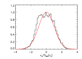
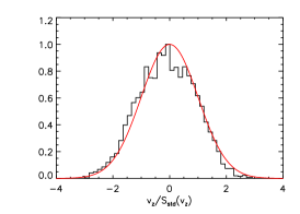
Figure 1: Histograms showing the distribution of individual line-of-sight velocities of all cluster members contained in a cylinder of projected radius $R_{200}$ along each selected axis, for all the 73 simulated clusters, and for three possible orientations of the simulation box along the line of sight (x, y and z axes). The red line corresponds to a Gaussian profile with the same mean and variance of the full sample.

In order to carry out the proposed analyses, we use a sample of 73 simulated massive clusters selected from the simulations described in Munari et al. (2013). The original, full sample contains about 300 cluster-sized or group-sized structures with masses $M_{200}>10^{13}M_{\odot}$. Here, our selected sample corresponds to all clusters located at five redshifts ($z=0.12,0.36,0.46,0.6,0.82$), and with masses $M_{200}>2\times 10^{14}M_{\odot}$.

The simulations were generated in $29$ Lagrangian regions, centred around the massive haloes identified in a parent, large-volume simulation box of $1$ h^-1 Gpc a side, and then re-simulated with higher resolution. The simulation starts in the initial conditions described in Bonafede et al. (2011), and was carried out in two subsequent steps, at different resolutions. The entire simulation was performed using the hydro-dynamical GADGET-3 code (Springel et al. 2001a). Gravitational forces are simulated using the TreeePM method, in which the Plummer-equivalent softening length $\epsilon=5$ h^-1 kpc is assumed in physical units for $z<2$ and fixed in comoving units for $z>2$. This simulation follows the evolution of $1024^{3}$ dark matter (DM) particles with mass $m_{\rm DM}=8.47\times 10^{8}$ h^-1 $M_{\odot}$ and the same number of gas particles with initial mass $m_{\rm gas}=1.53\times 10^{8}$ $M_{\odot}$, assuming the $\Lambda$-CDM cosmological model with $\Omega_{\rm DM}=0.24$, $\Omega_{\rm b}=0.04$, $\Omega_{\Lambda}=0.72$, $H_{0}=72$ km s^-1 Mpc^-1, $\sigma_{8}=0.8$, and $n_{\rm S}=0.96$.

Concerning the simulation model, we use the “AGN” simulation set described in Munari et al. (2013). This is a set of radiative simulations which account for the effect of star formation and the feedback triggered by both supernova explosions (SNe) and active galactic nuclei (AGN). Radiative cooling rates are computed following Wiersma et al. (2009). The prescription by Tornatore et al. (2007) is used to include metal enrichment of the intra-cluster medium (ICM) due to SNe (both type II and Ia) and asymptotic giant branch (AGB) stars, taking also into account the Chabrier (2003) initial mass function (IMF) for the stars population. For a more accurate description of the simulations and the different prescriptions, see Munari et al. (2013) and Rasia et al. (2015).

The bounded structures were identified first through a Friend-of-Friend (FoF) algorithm. Then, the identifications were refined using the SUBFIND algorithm (Springel et al. 2001b; Dolag et al. 2009). The DM sub-haloes identified in this way that contains stellar structure are considered ”galaxies”. In analogy with Munari et al. (2013), in this work we consider only galaxies containing a bounded stellar mass $3\times 10^{9}\,M_{\odot}$. This choice guarantees that we retain all sub-haloes more massive than $\sim 10^{11}\,M_{\odot}$. In total, there are $105,196$ galaxies in our sample of 73 clusters, being $17,433$ within the $R_{200}$ radius. Thus, on average we have $1440$ galaxies per cluster, being $239$ inside $R_{200}$.

3 Recipe for a bias-corrected Velocity Dispersion and Mass estimators in Galaxy Clusters

Using DM only or hydro-dynamical cosmological simulations, Evrard et al. (2008), Munari et al. (2013), and Saro et al. (2013) characterised scaling relations between GCs velocity dispersion of tracers, namely DM particles, sub-haloes and galaxies, and $M_{200}$:

$$\frac{\sigma_{\rm 1D}}{\mathrm{km\ s^{-1}}}=A\left[\frac{h(z)\ M_{200}}{10^{15}\ \mathrm{M}_{\odot}}\right]^{\alpha},$$ (1)

where $\sigma_{\rm 1D}\equiv\sigma_{\rm 3D}/\sqrt{3}$, and the 3D velocity dispersion, $\sigma_{\rm 3D}$, is calculated using all the DM particles or galaxies within a sphere of radius $R_{200}$, using the biweight estimator (Beers et al. 1990). However, DM particles, sub-haloes and galaxies lead to different values of parameters $A$ and $\alpha$ (Munari et al. 2013). Moreover, owing to the triaxiality of GCs and to the non-virialized state of some clusters, all the constraints for $\alpha$ are slightly different from the value $\alpha=1/3$ derived from the virial theorem.

In order to use GCs for cosmological studies, it is crucial to obtain an accurate, precise, and unbiased estimate for the velocity dispersion and, consequently, for the cluster masses. Among other possibilities, this goal could be achieved through spectroscopic follow-ups (e.g., Allen et al. 2011). Nevertheless, owing to observational limits, in real GC observations, it is very expensive to measure the line-of-sight velocity of all cluster members. In the new era of large galaxy cluster samples, where we often find galaxy cluster with a limited number of spectroscopic members ($N_{gal}\la 30$), it is important to characterise whether such a limited number of galaxies might lead to biased estimates of the velocity dispersion and/or the cluster mass.

The aim of this work is to characterise the statistical and physical biases both for velocity dispersion and mass estimates in the regime of small number of galaxies, and to provide a recipe to correct for them. As we explain below, the four basic steps of our proposed recipe are:

1. Evaluate the velocity dispersion of the cluster using an unbiased estimator;

2. Estimate the aperture radius and the mass fraction of the cluster members and correct for these sampling effects;

3. Estimate the fraction of interlopers that could contaminate the cluster members sample and correct the velocity dispersion;

4. Calculate the GC mass and correct for statistical biases introduced by the $\sigma$–$M$ relation.

In the following sections we demonstrate that these four steps represent a good way to estimate actual velocity dispersion and mass with samples containing low numbers of galaxy members.

4 Statistical Bias and Variance for Velocity Dispersion estimators

4.1 Velocity dispersion estimators and notation

Beers et al. (1990) presented a set of mean and scale estimators, and studied their efficiency in the presence of deviations from a Gaussian-distribution. In this paper, we decided to focus our attention on three of those estimators, namely the standard deviation, the biweight and the gapper. The standard deviation,

$${S_{\rm std}}({N_{\rm gal}})=\sqrt{\frac{1}{{N_{\rm gal}}-1}\sum_{i=1}^{{N_{\rm gal}}}(x_{i}-\mu)^{2}},$$ (2)

is defined as the lowest variance scale estimator for a Gaussian distribution. However, its dependence on $\mu$ (the mean of the distribution) makes it a non-robust estimator.

The biweight scale estimator is a function of the sample median (Tukey 1958), and it is defined as

$$S_{\rm bwt}({N_{\rm gal}})=\left(\frac{{N_{\rm gal}}^{2}}{{N_{\rm gal}}-1}\right)^{1/2}\frac{\left[\Sigma_{|u_{i}|<1}\,(x_{i}-M)^{2}\,(1-u_{i}^{2})^{4}\right]^{1/2}}{\left|\Sigma_{|u_{i}|<1}\,(1-u_{i}^{2})\,(1-5u_{i}^{2})\right|},$$ (3)

where the $u_{i}$ quantities are given by

$$u_{i}=\frac{(x_{i}-M)}{a\times\mathrm{MAD}}$$ (4)

with $a=9.0$, and $\mathrm{MAD}=\mathrm{median}\,(|x_{i}-M|)$ are the tuning constant and the median absolute deviation respectively. Finally, the gapper is a robust estimator (Wainer & Thissen 1976) based on the gaps of an order statistics, $x_{i},x_{i+1},\dots,x_{n}$. It is defined as a weighted average of gaps:

$$S_{\rm gap}({N_{\rm gal}})=\frac{\sqrt{\pi}}{{N_{\rm gal}}\,({N_{\rm gal}}-1)}\sum_{i=1}^{{N_{\rm gal}}-1}w_{i}\,g_{i},$$ (5)

where the gaps are given by

$$g_{i}=x_{i+1}-x_{i},\qquad i=1,\dots,{N_{\rm gal}}-1$$ (6)

and the (approximately Gaussian) weights are given by

$$w_{i}=i\,({N_{\rm gal}}-1).$$ (7)

For a more detailed description of these estimators see Beers et al. (1990). With the notation introduced in equations 2, 3 and 5, throughout this paper we will refer in a generic way to any of the three scale estimators as ${S_{\rm X}}({N_{\rm gal}})$, being X$=$ “std”, “bwt” or “gap”, for each one of the three cases.

4.2 Statistical bias and variance for the three estimators

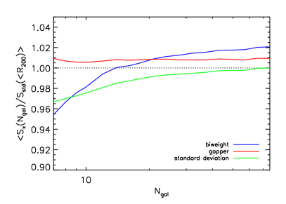
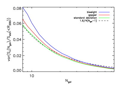
Figure 2: The mean velocity dispersion ${S_{\rm X}}/{S_{\rm std}}(<R_{200})$ as a function of the number of galaxies ${N_{\rm gal}}$ (left panel) and its variance (right panel), for our sample of 73 simulated galaxy clusters. The dispersion ${S_{\rm X}}({N_{\rm gal}})$ is calculated for the standard deviation (green line), biweight (blue line), and gapper (red line) estimators.

Our aim in this work is to characterise the statistical behaviour of the three aforementioned methods as a function of the number of galaxies, by quantifying the possible bias of each technique specifically in the small number of galaxies regime. As explained in Sect. 2, we use a set of 73 simulated GCs with redshifts $0.12\leq z\leq 0.82$ and masses $2\leq M_{200}/(10^{14}\,\mathrm{M}_{\odot})\leq 20$. Following the definition in Munari et al. (2013), we considered as galaxies only those DM subhaloes that contain a bounded stellar structure with a mass $\geq 3\times 10^{9}\,\mathrm{M}_{\odot}$.

We first characterise the distribution of velocities in our set of simulations. Figure 1 shows the histogram of the radial velocities for the 73 GCs along the three main projection axes, of all cluster members contained in a cylinder of projected radius $R_{200}$ along each selected axis. Even though these global distributions are apparently close to a Gaussian, each one of the 73 individual GC distribution is not, due to the present of substructures. A quantitative analysis shows that indeed there is a deviation from gaussianity in the overall distributions. In particular, we have estimated the following dimensionless parameter

$$c\equiv\frac{\langle x_{i}^{4}\rangle-\langle x_{i}^{2}\rangle^{2}}{\langle x_{i}^{2}\rangle^{2}},$$ (8)

which is related to the fourth moment of the distribution. We would expect $c=2$ for a perfect Gaussian sample. However, when evaluating the factor $c$ for each of the 73 clusters, we find a mean value $c=1.6\pm 0.4$ that implies a departure from a Gaussian of the simulated GC velocity distributions. As expected for relaxed clusters, the mean value of the $c$ parameter is found to be smaller than 2. The quoted error of $0.4$ corresponds to the scatter of the $c$ parameter over the 73 simulated clusters. As the statistical error in the determination of the $c$ parameter is significantly smaller than this value (on average, the number of galaxies within $R_{200}$ for each cluster is 239, so naively we would expected a statistical error of the order of $1/\sqrt{239}=0.065$ for one cluster, and less than $0.01$ for the ensemble of 73 clusters), this large scatter is reflecting the intrinsic variety of clusters properties in our simulations. We will use this $c$ parameter below, when estimating the variance of the three estimators.

We now evaluate the bias and the variance of the three scale estimators ${S_{\rm X}}({N_{\rm gal}})$. To do this, we have explored 20 different values for ${N_{\rm gal}}$, between ${N_{\rm gal}}=7$ and ${N_{\rm gal}}=75$, logarithmically spaced to better analyze the low-${N_{\rm gal}}$ tail. We have generated 2250 configurations by randomly selecting galaxies projected in a circle of radius $R_{200}$, 750 times for each main axis as line of sight and avoiding galaxy repetition. For each configuration, we estimated ${S_{\rm X}}({N_{\rm gal}})$ by repeating this procedure for each ${N_{\rm gal}}$ and for each galaxy cluster. The average values for ${S_{\rm X}}({N_{\rm gal}})$ are obtained by averaging the $73\times 2250$ velocity dispersions normalised with respect to ${S_{\rm std}}(<R_{200})$, which represents the velocity dispersion of all the galaxies in the simulation within a circle of projected radius $R_{200}$, and calculated using the standard deviation estimator. For completeness, we present in Table 1 the ratio of this relative bias when calculated with different estimators.

Table 1: Ratio of the relative bias ${S_{\rm X}}(<R_{200})/S_{\rm Y}(<R_{200})$ between two estimators X and Y, obtained with all the galaxies in the simulation within a circle of projected radius $R_{200}$.

X / Y	$BWT$	$GAP$	$STD$
$BWT$	$1.000$	$1.013\pm 0.009$	$1.021\pm 0.017$
$GAP$	$0.987\pm 0.008$	$1.000$	$1.008\pm 0.010$
$STD$	$0.980\pm 0.017$	$0.992\pm 0.010$	$1.000$

In the left panel of Fig. 2 we show how each estimator is able to recover the velocity dispersion, when compared to the standard deviation of the full sample ${S_{\rm std}}(<R_{200})$. By construction, for high ${N_{\rm gal}}$ (i.e., when using all galaxies in the simulation within $R_{200}$), the standard deviation estimator ${S_{\rm std}}({N_{\rm gal}})/{S_{\rm std}}(<R_{200})$ tends to one, while the other two estimators recover the asymptotic value given in Table 1.

In the low-${N_{\rm gal}}$ regime, all estimators are biased. The gapper (red line) returns an almost constant estimate of the velocity dispersion at any ${N_{\rm gal}}$, but that average value is slightly biased with respect to the true variance ($1.008\pm 0.010$, as shown in Table 1). The biweight shows a stronger dependence on the number of elements used for the estimation, specially in the low-${N_{\rm gal}}$ regime. In fact, for ${N_{\rm gal}}$ smaller than 30, it underestimates the true dispersion by up to $4$ % at ${N_{\rm gal}}=10$. A very similar behaviour is shown by the standard deviation estimator. We note that in this later case, the dependence on ${N_{\rm gal}}$ can be theoretically predicted, as showed in Appendix A, giving the analytic form $1-1/(4({N_{\rm gal}}-1))$. Based on this dependence on ${N_{\rm gal}}$, we have obtained a numerical fit to those curves in the left panel of Figure 2, using the following parametric equation:

$$1-\left(\left(\frac{D}{(N_{\rm gal}-1)}\right)^{\beta}+B\right).$$ (9)

Table 2 shows the best-fit values for the parameters $D$, $\beta$ and $B$, for each one of the three estimators (biweight, gapper and standard deviation).

Another crucial aspect for choosing a $\sigma_{v}$ estimator is its variance. We would expect the standard deviation to be the lowest variance estimator for a Gaussian distribution. We illustrate this in Appendix B, where we also show the behaviour of all three estimators in the same limit of Gaussian velocity distributions. For the more realistic case given by our set of numerical simulations, we confirm that this is also the case. The right panel of Fig. 2 shows the variance of the three estimators, $Var({S_{\rm X}}({N_{\rm gal}}))$, and it shows that the standard deviation has still the lowest variance. Moreover, we can compare this measured variance with the optimal one expected for the theoretical behaviour for a homogeneous population given by

$$Var({S_{\rm std}}({N_{\rm gal}})/{S_{\rm std}}(<R_{200}))=\frac{c}{4({N_{\rm gal}}-1)},\\$$ (10)

where the parameter $c$ was defined in equation 8. We find that the variance of the standard deviation is indeed very close to the optimal one, as well as the variance of the gapper. For low ${N_{\rm gal}}$ values ($\la 20$), the variance of the biweight estimator is significantly worse. Numerical fits to the dependence of the variance as a function of ${N_{\rm gal}}$ are given in Appendix C.

Using either the parametric fitting given in equation 9, or the numerical values from the left panel of Figure 2, we can now construct unbiased velocity dispersion estimators, by explicitly correcting for that statistical bias. We will use the primed notation ${S^{\prime}_{\rm X}}({N_{\rm gal}})$ when referring to these “corrected” estimators, which will be given by

$${S^{\prime}_{\rm X}}({N_{\rm gal}})\equiv{S_{\rm X}}({N_{\rm gal}})\left(1-\left(\left(\frac{D}{({N_{\rm gal}}-1)}\right)^{\beta}+B\right)\right)^{-1}$$ (11)

$$\approx{S_{\rm X}}({N_{\rm gal}})\left(1+\left(\left(\frac{D}{({N_{\rm gal}}-1)}\right)^{\beta}+B\right)\right).$$

and where the approximation in the second line uses the fact that the correction term is small compared to unity.

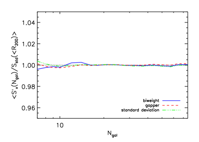
Figure 3: Mean (left panel) and variance (right panel) of the corrected estimators ${S^{\prime}_{\rm X}}({N_{\rm gal}})/S^{\prime}_{\rm std}(<R_{200})$, as a function of the number of galaxies ${N_{\rm gal}}$ in our sample of 73 simulated galaxy clusters, for the standard deviation (green line), biweight (blue line), and gapper (red line).

Table 2: Best-fit parameters to be used in the parametric function given in equation 9, describing the bias of the three estimators. See text for details.

	$BWT$	$GAP$	$STD$
$D$	$1$	$0$	$0.25$
$B$	$-0.0124\pm 0.0009$	$-0.0018\pm 0.0005$	$-0.0016\pm 0.0005$
$\beta$	$1.43\pm 0.01$	$1$	$1$

Figure 3 is equivalent to the Fig. 2, but now computed for the set of corrected estimators defined in equation 11. By construction, the new ${S^{\prime}_{\rm X}}({N_{\rm gal}})$ estimators are now unbiased (left panel), and their variance (right panel) have increased only by an small amount. As for the case of unprimed estimators, the corrected standard deviation is still the minimum variance estimator, although the three of them present very similar values for ${N_{\rm gal}}\ga 30$. For this reason, we decided to use $S^{\prime}_{\rm std}({N_{\rm gal}})$ as the reference estimator in the following sections, although we could in principle use any of the three estimators.

5 Bias from interlopers contamination

Galaxy clusters are not isolated structures in the Universe. This fact, together with the inevitable confusion associated to redshift-space measurements, implies that any spectroscopic sample of potential cluster members could be in principle contaminated. This population of pseudo cluster members, called “interlopers”, modifies the velocity distribution and therefore affects the estimation of the velocity dispersion (e.g. Wojtak et al. 2007, 2018; Pratt et al. 2019). Using numerical simulations of the entire visual cone, Mamon et al. (2010) showed that the fraction of galaxies outside the virial sphere that appear on sky projected within the virial radius could reach up to $\sim 27\,\%$, making the interlopers a potentially important source of error for an unbiased determination of the underlying velocity distribution. As shown below, the overall error due to interlopers is indeed similar or slightly larger than the statistical and physical biases discussed in this paper.

According to the definition of interlopers given in Pratt et al. (2019), it is useful to consider this population as the sum of two different types of objects: (i) galaxies gravitationally bounded to the clusters that are far from the cluster centre, but due to projection effects appear within a projected circle of a smaller radius (hereafter “type 1” interlopers); and (ii) background/foreground galaxies with similar redshifts to that of the cluster, but belonging to the large scale structure that surrounds the cluster itself (hereafter “type 2” interlopers). Note that, in our particular case of zoomed simulations, they are only including type 1 interlopers.

Providing a general recipe to correct the velocity dispersion bias of a given estimator due to the presence of interlopers is not possible, as in general the fraction of those objects will depend not only on ${N_{\rm gal}}$, but also on the particular criteria adopted for assigning cluster membership to galaxies observed in the cluster field, as well as the type of interlopers. Moreover, there are multiple methods in the literature for identifying interlopers, usually linked to specific cluster mass reconstruction methods. A very complete list can be found in Wojtak et al. (2018) and references therein. Unfortunately, none of those methods are capable of completely removing all contaminants (Wojtak et al. 2018), and moreover, these techniques have good results when applied to large galaxy samples (hundreds of members), but they are usually less effective when applied to smaller samples (tenths of members), as in the case of the caustic method (Diaferio 1999).

Here we limit our discussion to one particular member selection method, named the “sigma clipping”, and we illustrate the procedure to carry out the correction of the velocity estimation for the two types of interlopers. We emphasise that, in a general case, specific simulations will be required to quantify the bias associated to each particular method. The sigma clipping (Yahil & Vidal 1977) is one of the most used techniques for removing interlopers. This method clips galaxies whose radial velocity is above a certain threshold, being particularly effective in the external regions of the clusters.

5.1 Type 1 interlopers

We first estimate the impact of type 1 interlopers in our simulations. It is important to emphasise here that, throughout this paper, all our velocity dispersion quantities are computed using the galaxies contained in a cylinder of projected radius $R_{200}$. Thus, by construction, they will be affected by type 1 interlopers. In order to transform them into a velocity dispersion computed within a sphere of radius $R_{200}$, and therefore, free of type 1 interlopers, the average conversion factors that we find in our simulated sample are $0.990$, $0.981$ and $0.985$ for the biweight, gapper and standard deviation estimators, respectively. In summary, as a consequence of the presence of (type 1) interlopers, the velocity dispersion is overestimated between $1\%$ and $2\%$. This bias is relatively small, and comparable to the statistical biases discussed in the previous sections. In principle, it has to be corrected in the corresponding ${S^{\prime}_{\rm X}}$ estimators when transforming from velocity dispersion into masses, but only if the adopted $\sigma$–$M$ scaling relation from simulations did already account for the effect of type 1 interlopers.

Figure 4: Effect of type 1 interlopers on the velocity estimates, as a function of the number of galaxies, for the gapper estimator. The velocity dispersion $S_{\rm gap}({N_{\rm gal}})$ is computed first using the full galaxy sample (black solid line, equivalent to the red line in Figure 2), and then it is compared to the estimates after clipping the galaxy sample at $3$, $2.7$ and $2.5$ sigmas in the velocity space.

We further explore the possible correction of this bias using the sigma clipping method. Although this method might be effective in removing interlopers, cutting the tail of a distribution will necessarily introduce a bias in the estimation of the velocity dispersion. To quantify this effect, we tested four grades of clipping (no clip, $3\sigma$, $2.7\sigma$, $2.5\sigma$) in Figure 4 for one of the estimators. As expected, the higher the clip, the lower is the variance recovered by the estimator. However, it is interesting to note that this new bias partially alleviate the effect introduced by the type 1 interloper contamination. As in Mamon et al. (2010), we also find that both effects are compensated at around $2.7\sigma$, if we use the gapper to estimate the dispersion. However, we note that using the other two estimators, the clipping that compensate the effect of the interlopers is different. We find that a $2.5\sigma$ clipping for the biweight, and a $3\sigma$ clipping for the standard deviation compensates the effect of type-1 interlopers.

5.2 Type 2 interlopers

Figure 5: Combined effect of type 1 and 2 interlopers on ${S^{\prime}_{\rm X}}({N_{\rm gal}})/S_{\rm std}(<R_{200})$, as a function of the number of galaxies. The velocity dispersion, ${S^{\prime}_{\rm X}}({N_{\rm gal}})$, is first computed using the full galaxy sample (equivalent to the three colour lines shown in the left pannel of Figure 3). We also evaluated the response of biweight (blue), standard deviation (green), and gapper (red lines) using samples contaminated by a certain fraction of type 2 interlopers, as described in the text. By construction, our simulations also include the type 1 interlopers, as the velocity dispersion is estimated in the cylinder.

As explained above, here we use zoomed hydrodynamical simulations from a parent one, where the region of clusters are re-simulated at higher resolution. Although this technique is very useful to explore the appropriate mass range to form stars and galaxies, it has the disadvantage of re-simulating only a finite region around the centre of the cluster (in the case of study $\sim 5R_{200}$). Thus, all galaxies in our simulated catalogues are bounded to the cluster, and following our definition, they correspond to type 1 interlopers only.

To understand the effect introduced by type 2 interlopers, we have repeated the procedure described in the previous sub-section, but this time replacing some galaxies from the actual cluster distribution with random velocity values drawn from a uniform distribution in the velocity interval $[-2.7,2.7]\times{S_{\rm std}}(<R_{200})$. This uniform distribution is intended to mimic a field of background and foreground galaxies, in an extreme case of a velocity distribution which is completely different from that of the galaxies. Figure 5 presents the results obtained for five different fraction of interlopers: 5 % (dashed lines), 10 % (dot-dashed lines), 15 %(three dot-dashed lines), 20 % (long dashed lines), and 30 % (dotted lines). As expected, the inclusion of those type 2 interlopers produces a positive bias in the velocity dispersion, which at first order is found to be directly proportional to the relative fraction of interlopers. It is also noteworthy that all the three estimators are similarly affected by this “type 2” interloper contamination.

Although Fig. 5 shows a broad range of values for the fraction of type 2 interlopers, in real objects we would expect this number to be in the range of 5 to 10 % within a virial radius (Saro et al. 2013), being the fraction of type 1 objects significantly larger in number. If this is the case, then the effect of type 2 interlopers in the extreme case considered here will be at most 10 per cent. This is consistent with other results in the literature, which indeed present smaller values. For example, Mamon et al. (2010) showed that the the total fraction of interlopers in their simulations (including both types 1 and 2) is $\sim 27\%$, while their impact on the velocity estimation at $R_{200}$ is of the order of 2 %. Moreover, this effect is basically cancelled out in their final estimation of the velocity dispersion within $R_{200}$ when using the $2.7\sigma$ clipping, thus suggesting that the fraction of type 2 interlopers with a very different velocity distribution to the one of the true members is rather small. On the other hand, in our simulated cluster sample we find a median fraction of type 1 interlopers of $\sim 29\%$, which is consistent with the value of Mamon et al. (2010).

It is also important to note the strong dependence of type 2 interlopers with the sample aperture (Mamon et al. 2010; Saro et al. 2013), increasing rapidly beyond $R_{200}$. In practice, this makes the interloper contamination the most damaging effect for obtaining an unbiased velocity estimation for a single cluster for radii much larger than $R_{200}$.

Finally, we note that in real observations, the fraction of interlopers, and particularly type 2, will depend closely on the observational strategy and the particular algorithms and procedures used for member selection. Therefore, the effective number of contaminants cannot be estimated precisely with a general recipe. Studies such as Mamon et al. (2010); Saro et al. (2013) are necessary to statistically quantify their abundance in each particular observing strategy. As we are focused here in providing a general recipe for correcting the statistical and/or physical bias associated to the velocity estimators, we will not discuss further this effect. But we emphasise that for a reliable velocity estimation, the bias due to interlopers has to be taken into account and corrected specifically for each particular survey.

6 Physical Biases on velocity dispersion estimators

In the ideal case in which we can choose an uniformly selected sample of true cluster members inside $R_{200}$, the corrected set of scale estimators presented above will provide an unbiased estimation of the velocity dispersion of the cluster. However, observational strategies and technical limitations prevent us from reaching the ideal case. In this section we study two possible ways in which a particular selection of cluster members might produce biased velocity dispersion estimates.

6.1 Effects due to the selected fraction of massive galaxies

For a fixed integration time, the telescope aperture limits the detection magnitude and prevents us from detecting faint objects. In other cases, the technical requirements of spectrographs make it impossible to sample the cluster members adequately for arbitrary low brightness values. So, in practice, line-of-sight velocity samples contain only a fraction of GC members, generally the brightest objects in the GC, which are also the most massive. This fraction of objects is particularly small for high redshift GCs. In this subsection, we investigate if there is an induced bias due to this mass segregation.

In order to simulate this effect, we mimicked observational conditions by selecting three percentages of all visible galaxies in the simulation, i.e. 50 %, 33 %, and 25 %, by sorting the cluster members by mass and dividing the sample in 2, 3, and 4 mass bins, starting from the most massive object. For each case, as explained in Sect. 4, we averaged 2250 configurations (750 for each axis, $x$, $y$, $z$), considering numbers of galaxies between 8 and 75, avoiding galaxy repetition and evaluating the dispersion with the biweight, gapper, and standard deviation methods.

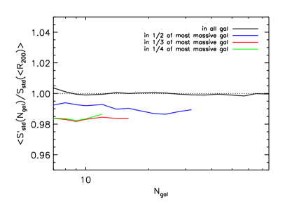
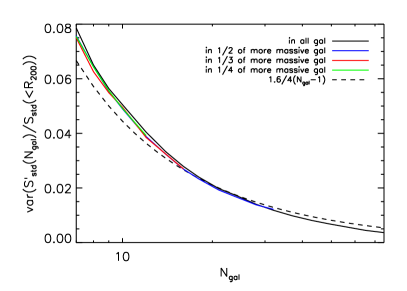
Figure 6: Left panel: Mean (bias) of $S^{\prime}_{\rm std}({N_{\rm gal}})/{S_{\rm std}}(<R_{200})$ as a function of the number of galaxies ${N_{\rm gal}}$, calculated by choosing galaxies within $100\%$ (black solid line), $1/2$ (blue solid line), $1/3$ (red solid line), and $1/4$ (green solid line) of the complete cluster member samples. Right panel: Variance of $S^{\prime}_{\rm std}({N_{\rm gal}})/{S_{\rm std}}(<R_{200})$ as a function of the number of galaxies ${N_{\rm gal}}$. The dashed line represents the theoretical expectation for the variance of the dispersion according to equation 10.

Figure 6 (left panel) shows $S^{\prime}_{\rm std}({N_{\rm gal}})/{S_{\rm std}}(<R_{200})$ as function of ${N_{\rm gal}}$ calculated with the corrected standard deviation estimator, and using galaxies picked up from 100 % (black line), $1/2$ (blue line), $1/3$ (red line) and $1/4$ (green line) of the complete cluster member samples. We see how a bias appears, with a nonlinear dependence with the fraction of massive galaxies considered in each case, but almost insensitive to the ${N_{\rm gal}}$ parameter. This means that the velocity dispersion is sensitive to the fraction of massive galaxies used to estimate it. In particular, taking into account only the most massive galaxies of the clusters ($1/4$ of the sample), one would find a velocity dispersion that could be underestimated up to 2 per cent. We can interpret this velocity bias in terms of a physical mechanism, the dynamical friction (Chandrasekhar 1943), which mostly affects the most massive galaxies, so that the velocity dispersion is lower with respect to that obtained using objects randomly selected from the complete galaxy sample. Table 3 shows the average bias of the primed estimators ${S^{\prime}_{\rm X}}$, calculated with respect to the full set of cluster members within $R_{200}$ (i.e., ${S_{\rm std}}(<R_{200})$), for each fraction in exam, and for the three estimators (biweight, gapper, and standard deviation). As this physical bias is almost independent on ${N_{\rm gal}}$, we could in principle use directly those values to produce a new corrected (unbiased) estimator.

Table 3: Relative bias of the primed estimators due to the selected fraction of massive galaxies. We evaluate it as the average $\left<{S^{\prime}_{\rm X}}/{S_{\rm std}}(<R_{200})\right>$ for all possible ${N_{\rm gal}}$ values.

Fraction	$BWT$	$GAP$	$STD$
$1$	$1.013$	$1.008$	$1$
$1/2$	$1.004$	$0.999$	$0.990$
$1/3$	$0.996$	$0.992$	$0.981$
$1/4$	$0.992$	$0.993$	$0.982$

In the right panel of Figure 6 we show the variance of $S^{\prime}_{\rm std}({N_{\rm gal}})/{S_{\rm std}}(<R_{200})$. The fraction of massive galaxies does not significantly affect the dispersion estimator variance.

6.2 Effect of aperture sub-sampling

All the analyses presented above include galaxies from the complete sample of cluster members, or a fraction of them, but the sample always being selected within $R_{200}$. However, there is already evidence in the literature that the velocity dispersion estimate needs to be corrected if galaxies are not sampled out to the cluster’s virial radius (e.g., Mamon et al. 2010; Sifón et al. 2016). In this subsection, we want to see how the selection region affects the $\sigma_{v}$ estimate in our simulations, by characterising the physical bias introduced when evaluating the velocity dispersion enclosed in a radius $r$ from the galaxy cluster center. In particular, we compute the velocity dispersion using all the galaxies inside a cylinder of variable radius $0.2\leq r/R_{200}\leq 1.5$. In addition, we average over all 73 simulated GCs and construct the $\left<{S^{\prime}_{\rm X}}(<r)/{S_{\rm std}}(<R_{200})\right>$ as a function of the $r/R_{200}$ profile (red line Fig. 7). The corresponding numerical values are given in Table 4. The velocity dispersion is (on average) overestimated where the region explored by the spectroscopic sample is smaller than $R_{200}$. The results are consistent with those obtained by Sifón et al. (2016) when using the biweight estimator for both ${S^{\prime}_{\rm X}}(<r)$ and ${S^{\prime}_{\rm X}}(<R_{200})$ (see Figure 4 and Table 3 in that paper).

We finally evaluate the combined effect of this aperture sub-sampling and the selection effect of a fraction of massive galaxies discussed in the previous subsection. We performed the same analysis described above for eight fractions of $R_{200}$, i.e. $r/R_{200}=0.2$, $0.3$, $0.4$, $0.5$, $0.8$, $1.0$, $1.2$ and $1.5$, and considering also different fractions of massive members. Unfortunately, we were unable to calculate the dispersion for the smaller fractions for radii less than half $R_{200}$ for our simulation set because not all the simulated clusters contain at least seven galaxies in these inner regions. But for larger radii ($r\ga R_{200}$), we find that the bias caused by the used fraction of massive galaxies remains almost constant at all radii. Therefore, we can apply the correction factors presented in Table 3, in combination with the radial correction profile shown in Figure 7 and in Table 4, to correct simultaneously for both effects.

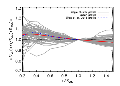
Figure 7: Average velocity dispersion profile within a given enclosed radius $r$, $<S^{\prime}_{\rm std}(<r)/{S_{\rm std}}(<R_{200})>$, normalised to $R_{200}$. The red line represents the mean at each radius of the individual 73 simulated GC profiles (grey lines). The numerical values are given in Table 4. The dashed blue line represents the Sifón et al. (2016) profile, which is almost coincident with our derived profile.

Table 4: Average velocity dispersion profile within a given enclosed radius $r$, $<S^{\prime}_{\rm std}(<r)/{S_{\rm std}}(<R_{200})>$, normalised to $R_{200}$. Values computed from the simulations. Uncertainties are the standard deviation.

$r/R_{200}$	$S^{\prime}_{\rm std}(<r)/{S_{\rm std}}(<R_{200})$
$0.2$	$1.044\pm 0.128$
$0.3$	$1.051\pm 0.106$
$0.4$	$1.047\pm 0.089$
$0.5$	$1.036\pm 0.071$
$0.6$	$1.030\pm 0.053$
$0.7$	$1.020\pm 0.039$
$0.8$	$1.012\pm 0.026$
$0.9$	$1.005\pm 0.015$
$1.0$	$0.998\pm 0.001$
$1.1$	$0.992\pm 0.016$
$1.2$	$0.986\pm 0.024$
$1.3$	$0.982\pm 0.034$
$1.4$	$0.978\pm 0.042$
$1.5$	$0.973\pm 0.045$

7 Bias in the mass estimation

7.1 Statistical bias in the estimation of $M_{200}$

In the previous sections we have studied how velocity dispersion estimators can be affected by different statistical and physical factors, and we have quantified the expected bias in those cases. In this section, we now show how mass estimators are also affected by the same effects.

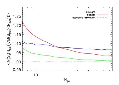
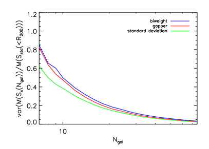
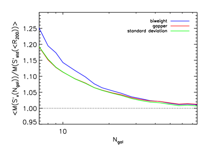
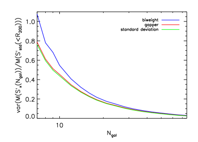
Figure 8: Mean (left panels) and variance (right panels) of $M\left({S_{\rm X}}({N_{\rm gal}})\right)/M\left({S_{\rm std}}(<R_{200})\right)$ and $M\left(S^{\prime}_{x}({N_{\rm gal}})\right)/M\left(S^{\prime}_{\rm std}(<R_{200})\right)$, which represent the standard mass estimator, eq. 12, applied to normal and unbiased velocity dispersion estimators, standard deviation (green), gapper (red), and biweight (blue). The theoretical expectation for $M\left({S_{\rm std}}({N_{\rm gal}})\right)/M\left({S_{\rm std}}(<R_{200})\right)$ is represented with the black dashed line.

The mass of a GC is not a direct observable. When we estimate the cluster mass using velocity dispersion estimates, we basically apply a function $M$–$\sigma_{\rm 1D}$ that has been previously calibrated either in simulations or using observations. Any non-linear transformation of $\sigma_{\rm 1D}$ will introduce a bias similar to the one that we have discussed for the $S_{\rm X}$ estimators, which will be more significant in the low-${N_{\rm gal}}$ regime.

Following equation 1, once we have obtained an estimate of the velocity dispersion (${S_{\rm X}}$), the mass of the cluster can be computed as

$$\frac{M({S_{\rm X}})}{10^{15}\,\mathrm{M}_{\odot}}=\left(\frac{{S_{\rm X}}}{A}\right)^{\frac{1}{\alpha}}.$$ (12)

with parameters $A=1177.0$ km s^-1 and $\alpha=0.364$ constrained by Munari et al. (2013) using the biweight as velocity dispersion estimator.

However, and in analogy to what we have seen in Sect. 4, even if we use an unbiased estimator for the velocity dispersion, and due to the fact that equation 12 contains a non-linear function of the variance, we expect a statistical bias with some dependence at low ${N_{\rm gal}}$. Using the results from Appendix A, as the transformation to obtain the mass is of the type $f(v)\propto v^{1/(2\alpha)}$ with $1/\alpha\sim 3$, we can predict the amount of bias.

As for the study of the dispersion estimators, in the case of mass estimators we also select as the reference velocity dispersion that one estimated with the standard deviation using all the galaxies within $R_{200}$. In the top row of Fig. 8 we show the results of the bias (left panel) and associated variance (right panel) of the mass estimator based on eq. 12, using ${S_{\rm X}}({N_{\rm gal}})$ as the velocity estimator. This case is noted as $\left<M({S_{\rm X}})/M({S_{\rm std}}(<R_{200}))\right>$, and $M({S_{\rm std}}(<R_{200}))$ represents the mass obtained using eq. 12 for the input value of ${S_{\rm std}}(<R_{200})$.

We see that this mass estimator $M({S_{\rm std}})$ is positively biased by a factor

$$\frac{1-2\alpha}{4\alpha^{2}({N_{\rm gal}}-1)},$$ (13)

as predicted by equation 28 in Appendix A. In a similar way, the $M(S_{\rm bwt})$ (blue line) and $M(S_{\rm gap})$ (red line) mass estimators are also biased positively biased.

For comparison, the bottom row of Fig. 8 shows the equivalent results of the bias (left panel) and associated variance (right panel) of the mass estimator but now using ${S^{\prime}_{\rm X}}({N_{\rm gal}})$ as the input velocity estimation. These quantities are represented as $\left<M({S^{\prime}_{\rm X}})/M({S_{\rm std}}(<R_{200}))\right>$. As anticipated, even if we use an unbiased velocity dispersion estimator, the non-linearity of the mass–velocity dispersion relation results in a biased mass estimate. It is interesting to note that the velocity dispersion bias is propagated into the mass bias, as seen by comparing the top and bottom panels on that figure. On one hand, as the $S_{\rm gap}$ is independent from ${N_{\rm gal}}$, in the transformation from the normal estimator to the bias-corrected one the only thing that changes is the normalisation (i.e. a constant factor, and therefore, the variance does not increase). On the other hand, the mass bias of ${S_{\rm std}}$ (top panel) is mitigated by the fact that the normal standard deviation tends to underestimate the velocity dispersion at low ${N_{\rm gal}}$. This effect is not present in the $M(S^{\prime}_{\rm std})$ profile (bottom panel) because $S^{\prime}_{\rm std}$ is, by construction, unbiased. Focusing our attention on the variance of these mass estimators, shown in the right panels of Fig. 8, we see that for $M({S_{\rm X}})$ (top panel), the standard deviation has the lowest variance, whereas the gapper and biweight show almost the same behaviour as functions of ${N_{\rm gal}}$. Instead, in the bottom panel the three $Var(M({S^{\prime}_{\rm X}}))$ functions show a behaviour similar to what we see for the dispersion estimators. The gapper variance remains almost untouched, and the standard deviation behaves like the gapper, whereas the biweight has the higher variance.

As done in Sect. 4, we have proposed a parametric description of the bias as a function of ${N_{\rm gal}}$, based on the analytic form of the bias for the standard deviation case. We also use here three parameters ($E$,$F$ and $\gamma$) in order to apply it to the gapper- and biweight-based mass estimators:

$$\frac{1-E\alpha}{(E\alpha)^{2}({N_{\rm gal}}-1)^{\gamma}}+F$$ (14)

The best-fit parameters describing the bias for the unprimed $M({S_{\rm X}})$ and primed $M({S^{\prime}_{\rm X}})$ mass estimators are listed in Tables 5 and 6, respectively.

Once we have fitted for this bias, we can propose bias-corrected mass estimators for those two cases, by defining

$$M^{\prime}\left({S_{\rm X}}({N_{\rm gal}})\right)=M\left({S_{\rm X}}({N_{\rm gal}})\right)\left[\frac{1-E\alpha}{(E\alpha)^{2}(N_{\rm gal}-1)^{\gamma}}+F\right]^{-1}$$ (15)

$$M^{\prime}\left({S^{\prime}_{\rm X}}({N_{\rm gal}})\right)=M\left({S^{\prime}_{\rm X}}({N_{\rm gal}})\right)\left[\frac{1-E^{\prime}\alpha}{(E^{\prime}\alpha)^{2}(N_{\rm gal}-1)^{\gamma^{\prime}}}+F^{\prime}\right]^{-1}.$$ (16)

Following the same convention for the notation adopted in previous sections, hereafter these bias-corrected estimators are represented with a “prime”, i.e. $M^{\prime}({S_{\rm X}}({N_{\rm gal}}))$ and $M^{\prime}({S^{\prime}_{\rm X}}({N_{\rm gal}}))$.

Table 5: Best-fit parameters for the function describing the bias in $\left<M({S_{\rm X}})/M({S_{\rm std}}(<R_{200}))\right>$ for simulated clusters, as described in equation 14.

	$BWT$	$GAP$	$STD$
$E$	$2.36\pm 0.06$	$1.49\pm 0.03$	$1.97\pm 0.07$
$F$	$0.058\pm 0.004$	$0.023\pm 0.002$	$0.003\pm 0.002$
$\gamma$	$0.7\pm 0.1$	$1.17\pm 0.04$	$1.15\pm 0.09$

Table 6: Best-fit parameters for the function describing the bias in $\left<M({S^{\prime}_{\rm X}})/M({S_{\rm std}}(<R_{200}))\right>$ for simulated clusters, as described in equation 14.

	$BWT$	$GAP$	$STD$
$E^{\prime}$	$1.31\pm 0.03$	$1.50\pm 0.03$	$1.53\pm 0.03$
$F^{\prime}$	$0$	$0$	$0$
$\gamma^{\prime}$	$1.24\pm 0.03$	$1.17\pm 0.04$	$1.11\pm 0.04$

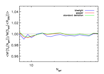
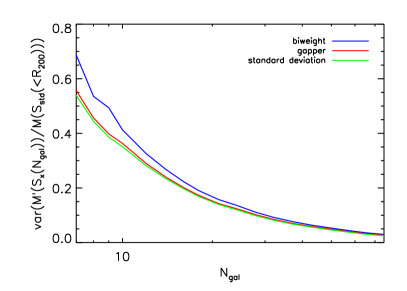
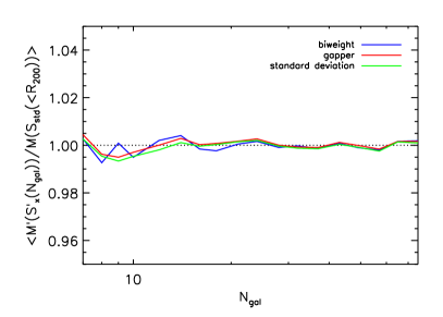
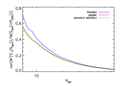
Figure 9: Mean (left panels) and variance (right panels) of the unbiased mass estimators $M^{\prime}({S_{\rm X}})/M^{\prime}({S_{\rm std}}(<R_{200}))$ (top row) and $M^{\prime}({S^{\prime}_{\rm X}})/M^{\prime}(S^{\prime}_{\rm std}(<R_{200}))$ (bottom row). In all panels, we show the results for the standard deviation (green), gapper (red), and biweight (blue) estimators.

Fig. 9 shows the bias and variance of $M^{\prime}({S_{\rm X}})$ (top panel) and $M^{\prime}({S^{\prime}_{\rm X}})$ (bottom panel). Both estimators are actually unbiased by construction. Concerning their variance, as expected, the biweight has the largest variance, whereas standard deviation behave similarly to the gapper but sill remaining as the lowest variance estimator. Analytical fits to the dependence of the variance as a function of ${N_{\rm gal}}$ are given in Appendix C.

7.2 Physical biases in the $M_{200}$ estimation

In Sect. 6 we explained how biases in velocity dispersion estimation could appear by taking into account only the more massive cluster members of the cluster, or by sampling a fraction of the virial radius $R_{200}$. These biases due to the physics of galaxy clusters are also propagated to the mass estimation.

In the top panels of Fig. 10 we show how choosing galaxies from the subset of the most massive ones also introduces a bias the mass estimation. For illustration purposes, we show the effect on the $M^{\prime}({S_{\rm X}})$ estimator only, but a similar figure can be generated for $M^{\prime}({S^{\prime}_{\rm X}})$. We find that the mass could be underestimated up to a $5\,\%$ when using $1/4$ of the sample containing the most massive galaxies. It is clear that the small biases in the velocity estimation are now amplified, especially at low ${N_{\rm gal}}$.

The aperture effect on the mass estimators is also shown in the bottom panel of Fig. 10. Also in this case, all the biases are, as expected, bigger than in the case of the velocity dispersion with a profile that prevents steeper sampling going to bigger apertures. From the variance point of view it increases in the core of the cluster and remains almost untouched for $r\geq R_{200}$.

It is evident that, owing to the high variance of the mass estimation, the combination of these effects may be considered negligible for a single cluster mass determination, but in order to determine the mean bias of a scale relation it is very important to obtain the most accurate mass estimation possible.

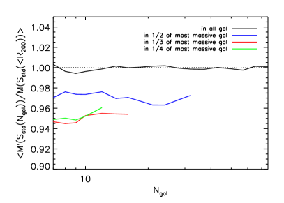
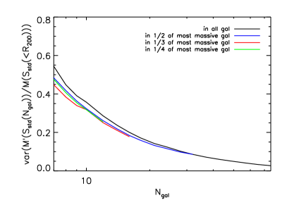
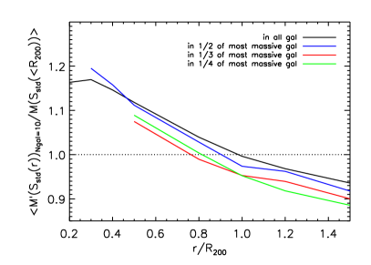
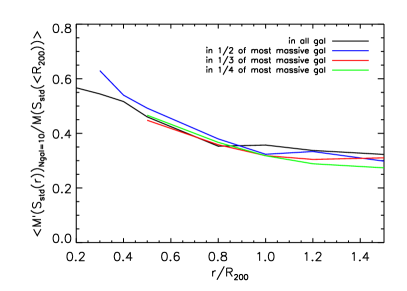
Figure 10: Mean and variance of the $M^{\prime}({S_{\rm X}})/M^{\prime}({S_{\rm std}}(<R_{200}))$ mass estimator, as a function of the number of galaxies ${N_{\rm gal}}$ (top panels), and as a function of the aperture radius $r$ (bottom panels). In black, blue, green, and red are represented the fraction that includes $100\%$, $1/2$, $1/3$ and $1/4$ of the most massive galaxies, respectively.

8 Applying corrections to a realistic case

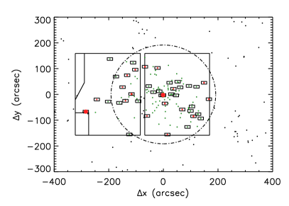
Figure 11: Left panel: Example of DOLORES/TNG simulated mask. Right panel: Example of OSIRIS/GTC simulated mask. See text for details. Black and green dots represent cluster members outside or inside the telescope field of view, respectively. Black rectangles are the slitlets, and the red points those considered line-of-sight velocity measurements (the symbol size is proportional to the mass of each galaxy with respect to the most massive one in the mask). The circle in dotted line represents the projected $R_{200}$ radius.

In this section, we show how well we can retrieve a bias-corrected velocity dispersion and mass estimation for a simulated sample of galaxy clusters under realistic observing conditions, but where only type 1 interlopers are considered. We follow the methodology outlined in Sect. 3 and discussed in the previous sections. The basic steps are:

1. Use the unbiased estimator ${S^{\prime}_{\rm X}}$, defined in equation 11, to estimate the cluster velocity dispersion.

2. Correct this velocity dispersion for the two physical effects (mass fraction and sampling aperture) described in the text, using Table 3 (or Fig. 6) and Table 4 (or Fig. 7), respectively. The second correction requires a first-order estimation of $R_{200}$, which can be obtained from the ${S^{\prime}_{\rm X}}$ value from the previous step and the $\sigma_{200}$–$M_{200}$ relation in equation 1.

3. Estimate the percentage of contaminants (interlopers) of the cluster members sample and correct, if needed, the velocity dispersion using the curves in Fig. 5. This provides the final velocity dispersion estimate, corrected for all effects described in the paper.

4. Compute the galaxy cluster mass by using the unbiased mass estimator $M^{\prime}({S^{\prime}_{\rm X}})$ defined in equation 16, and using as input the corrected ${S^{\prime}_{\rm X}}$ value from the previous step.

To perform this test, we decided to mimic the observational strategy that we adopted in our Planck PSZ1 follow-up program carried out during a two-year International Time Project (ITP13B/15A) (Planck Collaboration Int. XXXVI 2016; Barrena et al. 2018). This observational program has the aim of validating and characterising the unknown Planck SZ sources of the PSZ1 catalog in the northern hemisphere. To do this we used the DOLORES and OSIRIS spectrographs at the 3.5 m Telescopio Nazionale Galileo (TNG) and the 10.4 m Gran Telescopio Canarias (GTC) respectively, both located at Roque de los Muchachos Observatory (La Palma, Spain).

These facilities allow multi-object spectroscopy (MOS) observations that fit very well with our aim. However, the high number of clusters to be observed (about 200) and the need to obtain spectroscopy of very faint objects, ${}^{\prime}r_{\rm mag}>22$, did not allow us to use more than one MOS mask or a couple of long slits per cluster. For this reason we could only obtain a reduced number of cluster members, ${N_{\rm gal}}<40$. Our observational strategy started with the photometric redshift estimation. Once the $z_{\rm phot}$ was determined, we divided the GC sample into two redshift bins, $z\leq 0.4$ and $z>0.4$, in order to observe them at the TNG and the GTC respectively. Here, we mimic the galaxy selection procedure and the resultant galaxy catalogs. Owing to the different fields of view (FOV) of the two instruments and the differences in the two-mask designer software, we decided to implement both configurations following the same prescription as described above. In Fig. 11 we show two examples of a TNG and GTC mask scheme. There are some differences in the two configurations: i) TNG masks are always centered on the GC center while GTC masks, owing to the gap between the two CCD, are shifted $\sim 100"$ to the left; ii) the GTC mask designer tool is more precise than the TNG one. For this reason the minimum distance between galaxies is $5.4"$ and $8"$ for GTC and TNG masks respectively.

In order to simulate a cluster observation, we select each cluster at a random orientation and fraction of visible galaxies. Also, to mimic observational issues such as spectral contamination or wrong mask centering, we set a random number of slits as the effective catalog of measured radial velocities. We repeated this procedure to obtain $100$ mock samples out of the $73$ GCs object simulated in this study. For each of these samples we calculated the mean ratio between the estimated and the reference cluster velocity dispersion. Because the parameters of the scaling relation between $\sigma_{200}$–$M_{200}$, eq. 1, were constrained using the biweight estimation of the velocity dispersion, $S_{\rm bwt}(<R_{200})$, we decided to use it as a reference velocity dispersion for this analysis. For each of these samples we calculated the mean ratio between the estimated and the reference velocity dispersion of each cluster. Averaging over all the mock samples we obtained

$$\begin{split}\left<S_{\rm bwt}({N_{\rm gal}},r)/S_{\rm bwt}(<R_{200})\right>&=0.96\pm 0.03,\\ \left<S_{\rm gap}({N_{\rm gal}},r)/S_{\rm bwt}(<R_{200})\right>&=0.99\pm 0.03,\\ \left<{S_{\rm std}}({N_{\rm gal}},r)/S_{\rm bwt}(<R_{200})\right>&=0.96\pm 0.02.\end{split}$$ (17)

Using the estimators ${S^{\prime}_{\rm X}}$ defined in eq. 11 with the parameters in Table 2, we corrected the bias due to the number of galaxies. To correct the biases due to the GC physics, the first step is to identify in which fraction of massive galaxies the detected cluster members reside. The second step is to calculate the aperture radius, which is the sampling radius. To do this, first we needed to estimate $R_{200}$. Based on a first estimate of the cluster mass using ${S_{\rm X}}({N_{\rm gal}})$, we can derive a first-order approximation to that radius, noted as $R^{\rm X}_{200}$. This value is used to apply the aperture correction shown on the right panel of Fig. 7 to ${S^{\prime}_{\rm X}}$. In our case, each velocity dispersion was corrected individually after averaging over all the clusters, and then averaging over all the $100$ configurations to obtain

$$\begin{split}\left<S^{\prime}_{\rm bwt}(N_{\rm gal},r)/S_{\rm bwt}(<R_{200})\right>&=1.00\pm 0.03,\\ \left<S^{\prime}_{\rm gap}(N_{\rm gal},r)/S_{\rm bwt}(<R_{200})\right>&=1.00\pm 0.02,\\ \left<S^{\prime}_{\rm std}(N_{\rm gal},r)/S_{\rm bwt}(<R_{200})\right>&=1.00\pm 0.02,\end{split}$$ (18)

which represent bias-corrected estimates of the velocity dispersion. We note that these quantities are referred to the velocity dispersion computed in the cylinder $S_{\rm bwt}(<R_{200})$, and thus they include type 1 interlopers as described in Sect. 5.1. If we want to correct those values from this effect, we have to multiply those values by the corrections factors quoted in that subsection, i.e., $0.990$, $0.981$ and $0.985$ for the biweight, gapper and standard deviation estimators, respectively.

Using these velocity dispersion, we can now calculate the cluster masses, $M({S^{\prime}_{\rm X}})$, obtaining

$$\begin{split}\left<M\left(S^{\prime}_{\rm bwt}(N_{\rm gal},r)\right)/M\left(S_{\rm bwt}(<R_{200})\right)\right>&=1.17\pm 0.09,\\ \left<M\left(S^{\prime}_{\rm gap}(N_{\rm gal},r)\right)/M\left(S_{\rm bwt}(<R_{200})\right)\right>&=1.14\pm 0.08,\\ \left<M\left(S^{\prime}_{\rm std}(N_{\rm gal},r)\right)/M\left(S_{\rm bwt}(<R_{200})\right)\right>&=1.13\pm 0.07.\end{split}$$ (19)

As shown above, these masses are overestimated, and in order to correct for this bias, we have to use the primed mass estimator, $M^{\prime}$, as explained in Sec. 7.1. In this case, we obtain

$$\begin{split}\left<M^{\prime}\left(S^{\prime}_{\rm bwt}(N_{\rm gal},r)\right)/M^{\prime}\left(S_{\rm bwt}(<R_{200})\right)\right>&=1.00\pm 0.07,\\ \left<M^{\prime}\left(S^{\prime}_{\rm gap}(N_{\rm gal},r)\right)/M^{\prime}\left(S_{\rm bwt}(<R_{200})\right)\right>&=1.00\pm 0.07,\\ \left<M^{\prime}\left(S^{\prime}_{\rm std}(N_{\rm gal},r)\right)/M^{\prime}\left(S_{\rm bwt}(<R_{200})\right)\right>&=1.00\pm 0.06.\end{split}$$ (20)

It is also interesting to compare these mass estimates with the true mass, $M_{200}$ directly estimated from the simulation as the mass of all particles within $R_{200}$. Those values were used to constrain the parameters in equation 1 (Munari et al. 2013). The direct estimation of the velocity dispersion using ${S_{\rm X}}$ leads to a biased estimation of $M_{200}$:

$$\begin{split}\left<M\left(S_{\rm bwt}\,(N_{\rm gal},r)\right)/M_{200}\right>&=1.07\pm 0.09,\\ \left<M\left(S_{\rm gap}\,(N_{\rm gal},r)\right)/M_{200}\right>&=1.13\pm 0.08,\\ \left<M\left(S_{\rm std}\,(N_{\rm gal},r)\right)/M_{200}\right>&=1.03\pm 0.08,\end{split}$$ (21)

If the dispersion estimator is the corrected one, ${S^{\prime}_{\rm X}}$, we now retrieve a mass that is almost unbiased:

$$\begin{split}\left<M\left(S^{\prime}_{\rm bwt}\,(N_{\rm gal},r)\right)/M_{200}\right>&=1.18\pm 0.10,\\ \left<M\left(S^{\prime}_{\rm gap}\,(N_{\rm gal},r)\right)/M_{200}\right>&=1.13\pm 0.09,\\ \left<M\left(S^{\prime}_{\rm std}\,(N_{\rm gal},r)\right)/M_{200}\right>&=1.13\pm 0.08,\end{split}$$ (22)

Finally, $M^{\prime}$ provides the final, unbiased estimate of $M_{200}$:

$$\begin{split}\left<M^{\prime}\left(S^{\prime}_{\rm bwt}\,(N_{\rm gal},r)\right)/M_{200}\right>&=1.00\pm 0.08,\\ \left<M^{\prime}\left(S^{\prime}_{\rm gap}\,(N_{\rm gal},r)\right)/M_{200}\right>&=1.00\pm 0.07,\\ \left<M^{\prime}\left(S^{\prime}_{\rm std}\,(N_{\rm gal},r)\right)/M_{200}\right>&=0.99\pm 0.07,\\ \end{split}$$ (23)

Again, for this example these quantities are referred to a “true” mass computed from the velocity dispersion computed in the cylinder $S_{\rm bwt}(<R_{200})$. If we want to isolate the effect of type 1 interlopers, then the true $M_{200}$ has to be computed using the velocity dispersion in a sphere of radius $R_{200}$, and the primed velocity dispersion estimates will have to be corrected also for the same bias.

These numbers show that also in this realistic situation, the proposed set of corrected estimators are able to recover an unbiased estimate for both the velocity dispersion and mass of the galaxy clusters.

9 Conclusions

In this article, we have used 73 simulated GCs from hydrodynamic simulations with AGN feedback and star formation. We have taken into account three different estimators: the biweight, the gapper, and the standard deviation. We have focused on the limit of a low number of galaxy members (${N_{\rm gal}}<75$), and studied the bias and error (variance) of each estimator.

This study presents a detailed study of three techniques to estimate velocity dispersion quantifying possible biases brought about by their definition and observational limits. In a future paper, we shall apply the optimal technique with the corresponding corrections to a real sample of GCs in order to estimate bias-corrected dynamical masses and compare them with those evaluated using different proxies.

We propose a recipe with the aim of estimate reliable velocity dispersion and mass estimators with the lowest bias and variance as possible in the low-${N_{\rm gal}}$ regime. We constructed unbiased estimators based on the standard deviation, biweight, and gapper while correcting for their ${N_{\rm gal}}$ dependence, ${S^{\prime}_{\rm X}}$. In this case, we focused our attention on the variance of these estimators. Although asymptotically the three estimators have the same variance, in the range of a number of galaxies in which we are interested, ${N_{\rm gal}}<40$, the corrected biweight has an even higher variance with respect to the normal biweight and, consequently, with respect to the other two estimators. After the bias correction, we see that the variance of the standard deviation and gapper are compatible for ${N_{\rm gal}}\geq 20$, whereas for ${N_{\rm gal}}<20$ the corrected standard deviation is the lowest variance estimator.

We have also tested the robustness of the three ${S^{\prime}_{\rm X}}$ estimators when the galaxy sample is contaminated by interlopers, considering both gravitationally bound interlopers (type 1) and background/foregrounds galaxies (type 2). For type 1 interlopers, the bias in the velocity dispersion estimator is found to be $\sim 2$ %, comparable to the other statistical biases discussed above, and consistent with the results obtained by other authors which include also type 2 interlopers in their analysis (e.g. Mamon et al. 2010). This bias can be corrected using a $2.7\sigma$ clipping technique (Yahil & Vidal 1977). For type 2 interlopers, here we explored the conservative approach of assigning them a uniform velocity distribution, which is completely different from the true distribution of cluster members. Our results show that the three estimators are similarly affected, and that at first order, the bias in ${S^{\prime}_{\rm X}}$ is roughly proportional to the percentage of type 2 interlopers in our approach. Although comparable to the other effects discussed in this paper, the contribution of type 2 interlopers could provide the main bias in the velocity dispersion estimation, specially for radii beyond $R_{200}$, if their fraction is as large as 10 % (e.g. Saro et al. 2013). Finally, this fraction of type 2 contaminants depends on the particular GCs member selection procedure and, hence, can vary from survey to survey. Thus, a general formula based only on ${N_{\rm gal}}$ can not be provided.

We also studied how observational limitations influence the estimation of velocity dispersion in GCs. We recognised the most likely sources of bias in i) the selection effect due to the luminosity of GC members observed and hence in the fraction of massive galaxies used to estimate the velocity dispersion; ii) the aperture radius of the observation, and hence the fraction of the viral radius explored. We saw that the bias increased for the smaller fraction of massive galaxies. This bias was estimated to be around the $2\,\%$ when considering only $1/4$ of the more massive galaxies.

Regarding the effect produced by sampling aperture, we found that the maximum deviation was produced for an aperture radius of $0.3$–$0.4\,R_{200}$, which is in agreement with Sifón et al. (2016) results.

We also tested the mass estimators defined by eq. 1 with the parameters of Munari et al. (2013). In this case, we observed that all three estimators had a dependence on the number of galaxies, overestimating the reference mass at low ${N_{\rm gal}}$. The standard deviation profile can be analytically derived by taking into account the fact that the mass is a nonlinear function of the variance, as explained in Appendix A. Also, in this case, we defined a new set of mass estimators, $M({S_{\rm X}})$ and $M^{\prime}({S^{\prime}_{\rm X}})$, correcting the mass estimator applied to the biweight, gapper, and standard deviation, or to their corrected counterparts, respectively. We constructed these estimators to be unbiased over the entire range of ${N_{\rm gal}}$ and found that the mass estimator based on the standard deviation, whether corrected or not, was the lowest variance one.

The ultimate aim of this paper is not only to correct the velocity dispersion and mass estimates of a single cluster, but also to develop a method to obtain bias-corrected mean mass estimates in order to constrain the parameter of mass scaling relations. For this reason, we also applied these techniques to a set of mock observations to retrieve bias-corrected mean velocity dispersion and masses. These types of analyses will be of relevance for precision cosmology analyses with large samples of galaxy clusters, in the light of forthcoming results from space missions as eROSITA or EUCLID.

Appendix A Bias in the estimation of the nonlinear function of variance $g(v)$

If we assume a random variable $x$ with probability $p_{i}$, we can estimate any ordinary moment as:

$$E[x^{j}]=\sum_{i=1}^{N}x_{i}^{j}p_{i}.$$ (24)

The moment of second order is the variance, $E[Var(x)]=E[v]=<x^{2}>_{n}-<x>^{2}_{n}$, which is unbiased for any number of data, $N$.

In this appendix we explain how a bias is induced when a quantity is calculated as a nonlinear function of variance, $m=g(v)$. We evaluate $E[g(v)]$, which is the estimate of the function $g(v)$. We can use as the estimator of $m$ the function $g$ applied at the estimated value of $E[v]$,

$$E[g(v)]=g(E[v]).$$ (25)

The estimator $g(E[v])$ will be unbiased only if the function $g(v)$ is linear. In case that $m$ is a nonlinear function of the variance, e.g. standard deviation and mass, we can write the mean of $g(E[v])$ as:

$$<g(E[v])>\simeq g(v)+g^{\prime}(v)<\Delta E[v]>+\frac{1}{2}g^{\prime\prime}(v)<(\Delta E(v))^{2}>.$$ (26)

If the variable $v$ is unbiased, we can assume that $\left<\Delta E[v]\right>=0$ and

$$\left<(\Delta E[v])^{2}\right>=var(E[v])=\frac{2v^{2}}{N},$$ (27)

which implies that the unbiased estimate of $g(v)$ is

$$E[g(v)]=g(v)-\frac{1}{2}g^{\prime\prime}(v)\frac{2v^{2}}{N}.$$ (28)

In the case of the standard deviation $\sigma=v^{1/2}$ we have

$$E[\sigma]=\sigma+\frac{1}{4}\frac{\sigma}{n},$$ (29)

which is the unbiased standard deviation estimator.

Appendix B Statistical bias and variance for velocity dispersion and mass estimators in the limit of a Gaussian distributions

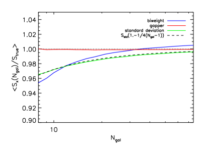
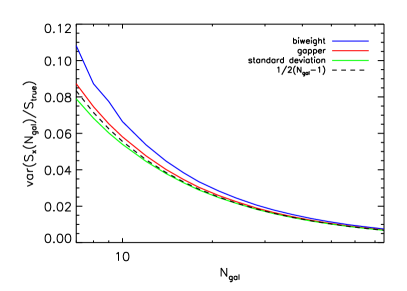
Figure 12: Mean (left panel) and variance (right panel) of ${S_{\rm X}}({N_{\rm gal}})$, as a function of the number of galaxies ${N_{\rm gal}}$, for the case of Gaussian-distributed random velocities. Green, red, and blue lines represent respectively the behaviour of the standard deviation, gapper, and biweight estimators.

In analogy to the cases discussed in the main text, in this appendix we show how the velocity dispersion and mass estimators presented above behave in the limit of a perfectly Gaussian velocity distribution. To this end, we generate 73 Gaussian distributions fixing the mean ($\mu=0$), and the dispersion $\sigma={S_{\rm true}}$, being ${S_{\rm true}}$ the dispersion corresponding to $M_{200}$ though eq. 1 for each cluster in this new simulated sample.

As in the main text, we explore 20 different values for ${N_{\rm gal}}$, between ${N_{\rm gal}}=7$ and ${N_{\rm gal}}=75$. We used $50\,000$ different configuration for each ${N_{\rm gal}}$ and each “cluster”, thus using $73\times 50\,000$ velocity dispersion estimates normalised with respect to ${S_{\rm true}}$. We note that by fixing the width of the Gaussian distribution, we avoid the need to select a reference estimator and, hence, we can investigate the absolute bias of each estimator with respect to the same ${S_{\rm true}}$ value.

B.1 Velocity dispersion estimators

Fig. 12 illustrates the behaviour of the (uncorrected) velocity estimators. We note that the gapper and the standard deviation recover the true velocity dispersion, asymptotically, for high ${N_{\rm gal}}$. However, this is not the case for the biweight estimator, which presents a small asymptotic bias. In the small number of galaxies limit, the behaviour of the three estimators is very similar to the one showed in Fig. 2. The standard deviation (green line) follows, as expected, the exact analytic profile derived in Appendix A, whereas the gapper (red line) shows to be an almost unbiased estimator for any value of ${N_{\rm gal}}$. Table 7 presents the best-fit values of the parameters $D$, $\beta$ and $B$ in equation 9, obtained now for this case of Gaussian velocity distributions.

Table 7: Best-fit parameters for the functions describing ${S_{\rm X}}({N_{\rm gal}})$ in the case of Gaussian velocity distributions.

	$BWT$	$GAP$	$STD$
$D$	$0.72\pm 0.03$	$0$	$0.25$
$B$	$-0.007\pm 0.001$	$0.0007\pm 0.0002$	$0$
$\beta$	$1.28\pm 0.03$	$1$	$1$

Concerning the variance, from a theoretical point of view we would expect the standard deviation to be the lowest variance estimator for a Gaussian distribution. This is confirmed in Fig. 12, which shows that as expected, the standard deviation follows the theoretical prescription given by

$$var({S_{\rm std}}({N_{\rm gal}}))=\frac{S_{\rm true}^{2}}{2({N_{\rm gal}}-1)}.$$ (30)

In this case of Gaussian velocity distributions, it is also interesting to test the response of the square of these three estimators $\left<{S_{\rm X}}^{2}({N_{\rm gal}})/S_{\rm true}^{2}\right>$, which in the case of the standard deviation corresponds to the variance. From a theoretical point of view, the variance is one of the ordinary moments of a distribution, and is not biased. Fig. 13 presents the results, confirming this well-known behaviour for the standard deviation, and showing that the other two estimators are clearly biased in this low ${N_{\rm gal}}$ regime. Also, the variance of the variance follows the expected analytic dependence for the standard deviation,

$$var({S_{\rm X}}^{2}({N_{\rm gal}}))=\frac{2S_{\rm true}^{4}}{(N_{\rm gal}-1)}.$$ (31)

We note that both the gapper and biweight have a similar dependence of the variance on ${N_{\rm gal}}$, being the biweight the estimator presenting a higher variance.

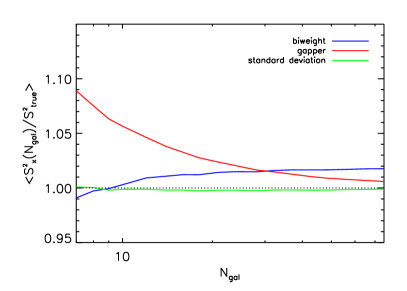
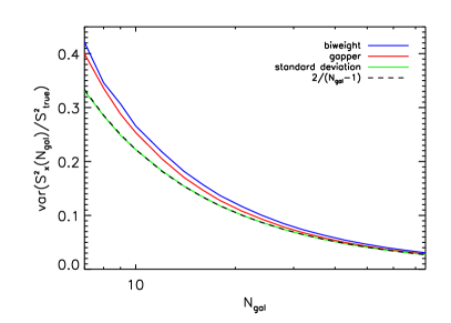
Figure 13: Mean (left) and variance (right) of ${S_{\rm X}}^{2}({N_{\rm gal}})$ as a function of the number of galaxies ${N_{\rm gal}}$, for the case of Gaussian random velocities. Green, red, and blue lines represent respectively the behaviour of the standard deviation, gapper, and biweight estimators.

Following the methodology applied in Sect. 4, we can construct the unbiased scale estimators ${S^{\prime}_{\rm X}}$. We have checked that this new set of corrected estimators ${S^{\prime}_{\rm X}}$, defined as in equation 11 and using the parameters listed in table 7, provide unbiased estimates for the velocity dispersion.

B.2 Mass estimators

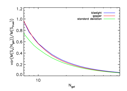
Figure 14: Mean (left) and variance (right) of $M\left({S_{\rm X}}({N_{\rm gal}})\right)/M(S_{\rm true})$ as a function of ${N_{\rm gal}}$, for the case of Gaussian random velocities. The dashed line in the left panel represents the expected analytic formula for the dependence of $F(S_{\rm std})$ on ${N_{\rm gal}}$ for the standard deviation described in Appendix A. Green, red, and blue lines represent respectively the behaviour of the standard deviation, gapper, and biweight estimators.

We now discuss the behaviour of the mass estimators in the case of Gaussian velocity distributions. Here, the reference true mass, $M({S_{\rm true}})$, is calculated applying eq. 1, using the parameters $A=1177.0$ km s^-1 and $\alpha=0.364$ from Munari et al. (2013). Fig. 14 illustrates the bias for the uncorrected mass estimator $M\left({S_{\rm std}}({N_{\rm gal}})\right)/M({S_{\rm true}})$. In general, the dependence on ${N_{\rm gal}}$ for all mass estimators is very similar to that in Fig. 8. In particular, the standard deviation mass estimator follows the theoretical analytic form presented in eq. 28. The right panel in the same figure shows the variance of $M\left({S_{\rm X}}({N_{\rm gal}})\right)/M({S_{\rm true}})$. Although we note a slightly higher variance at low ${N_{\rm gal}}$, the shape of variance profiles are similar to those presented in figure 8 for the real cluster simulations.

Table 8: Best-fit parameters of the functions $\left<M\left({S_{\rm X}}({N_{\rm gal}})\right)/M(S_{\rm true})\right>$ for Gaussian velocity distributions.

	$BWT$	$GAP$	$STD$
$E$	$2.22\pm 0.02$	$1.505\pm 0.007$	$2$
$F$	$0.023\pm 0.001$	$0.0013\pm 0.0005$	$0$
$\gamma$	$0.82\pm 0.04$	$1.088\pm 0.009$	$1$

Table 9: Best-fit parameters of the functions $\left<M\left({S^{\prime}_{\rm X}}({N_{\rm gal}})\right)/M({S_{\rm true}})\right>$ for Gaussian velocity distributions.

	$BWT$	$GAP$	$STD$
$E^{\prime}$	$1.28\pm 0.01$	$1.504\pm 0.007$	$1.521\pm 0.007$
$F^{\prime}$	$0.0078\pm 0.0008$	$0.0032\pm 0.0005$	$0.0009\pm 0.0005$
$\gamma^{\prime}$	$1.23\pm 0.01$	$1.088\pm 0.009$	$1.083\pm 0.008$

Bias-corrected mass estimators for Gaussian distributions, based both on the plain estimators ${S_{\rm X}}$, or their unbiased counterparts ${S^{\prime}_{\rm X}}$, can be obtained using equation 15 with the parameters listed in Tables 8 and 9, respectively. Similarly to the case of true velocity distributions, in this case of Gaussian velocities the biweight has also the largest variance, whereas standard deviation has the lowest one, with almost the same behaviour as the gapper.

Appendix C Analytical fit to the variance of the different estimators

Sect. 4.1 and equations 11, 15 and 16 present the definitions of different estimators for the velocity dispersion and the mass for galaxy clusters. For all these cases, figures 2, 3, 8 and 9 showed the mean and variance of the three estimators, as a function of ${N_{\rm gal}}$. Analytical expressions for the corrected estimators were given in the main text.

In some applications, it is useful to have also an analytical fit to the variance of those estimators. Here we provide this fit, using a common expression for all cases with only two free parameters:

$$Var=\frac{\epsilon}{4({N_{\rm gal}}-1)^{\beta}}.$$ (32)

Table 10 contains the the best-fit values for the $\epsilon$ and $\beta$ parameters for all those estimators. In general, the standard deviation estimator has the lowest variance in all cases, being the variance of the gapper also very close but slightly larger. The biweight estimator has a stronger dependence on ${N_{\rm gal}}$, specially in the low-${N_{\rm gal}}$ regime.

Table 10: Coefficient of the numerical fit to the dependence of the variance as a function of ${N_{\rm gal}}$ for different estimators.

Estimator	BWT	GAP	STD
$Var({S_{\rm X}})$	$\epsilon=3.69\pm 0.10$	$\epsilon=2.42\pm 0.05$	$\epsilon=2.05\pm 0.06$
	$\beta=1.24\pm 0.01$	$\beta=1.15\pm 0.01$	$\beta=1.11\pm 0.01$
$Var({S^{\prime}_{\rm X}})$	$\epsilon=4.63\pm 0.16$	$\epsilon=2.42\pm 0.05$	$\epsilon=2.36\pm 0.06$
	$\beta=1.33\pm 0.02$	$\beta=1.15\pm 0.01$	$\beta=1.15\pm 0.01$
$Var(M({S_{\rm X}}))$	$\epsilon=31.7\pm 1.1$	$\epsilon=34.4\pm 1.0$	$\epsilon=21.2\pm 0.5$
	$\beta=1.26\pm 0.02$	$\beta=1.32\pm 0.013$	$\beta=1.20\pm 0.01$
$Var(M({S^{\prime}_{\rm X}}))$	$\epsilon=61.0\pm 3.7$	$\epsilon=32.9\pm 0.9$	$\epsilon=32.1\pm 0.8$
	$\beta=1.50\pm 0.03$	$\beta=1.33\pm 0.01$	$\beta=1.33\pm 0.01$
$Var(M^{\prime}({S_{\rm X}}))$	$\epsilon=23.7\pm 0.8$	$\epsilon=16.7\pm 0.5$	$\epsilon=16.3\pm 0.5$
	$\beta=1.21\pm 0.01$	$\beta=1.13\pm 0.01$	$\beta=1.13\pm 0.01$
$Var(M^{\prime}({S^{\prime}_{\rm X}}))$	$\epsilon=23.9\pm 0.8$	$\epsilon=16.9\pm 0.5$	$\epsilon=16.2\pm 0.5$
	$\beta=1.21\pm 0.02$	$\beta=1.13\pm 0.01$	$\beta=1.13\pm 0.01$