Learning to Play Table Tennis From Scratch
using Muscular Robots

Abstract

Dynamic tasks like table tennis are relatively easy to learn for humans but pose significant challenges to robots. Such tasks require accurate control of fast movements and precise timing in the presence of imprecise state estimation of the flying ball and the robot. Reinforcement Learning (RL) has shown promise in learning of complex control tasks from data. However, applying step-based RL to dynamic tasks on real systems is safety-critical as RL requires exploring and failing safely for millions of time steps in high-speed and high-acceleration regimes. In this paper, we demonstrate that safe learning of table tennis using model-free Reinforcement Learning can be achieved by using robot arms driven by pneumatic artificial muscles (PAMs). Softness and back-drivability properties of PAMs prevent the system from leaving the safe region of its state space. In this manner, RL empowers the robot to return and smash real balls with $5\text{\,}\mathrm{m}\text{\,}{\mathrm{s}}^{-1}$ and $12\text{\,}\mathrm{m}\text{\,}{\mathrm{s}}^{-1}$ on average respectively to a desired landing point. Our setup allows the agent to learn this safety-critical task (i) without safety constraints in the algorithm, (ii) while maximizing the speed of returned balls directly in the reward function (iii) using a stochastic policy that acts directly on the low-level controls of the real system and (iv) trains for thousands of trials (v) from scratch without any prior knowledge. Additionally, we present HYSR, a practical hybrid sim and real training procedure that avoids playing real balls during training by randomly replaying recorded ball trajectories in simulation and applying actions to the real robot. To the best of our knowledge, this work pioneers (a) fail-safe learning of a safety-critical dynamic task using anthropomorphic robot arms, (b) learning a precision-demanding problem with a PAM-driven system that is inherently hard to control as well as (c) train robots to play table tennis without real balls. Videos and datasets of the experiments can be found on muscularTT.embodied.ml.

I Introduction

Reinforcement Learning (RL) solves challenging tasks such as the complex game of Go [1], full body locomotion tasks in simulation [2] or difficult continuous control tasks such as robot manipulation [3, 4] to name just a few. All of these challenging tasks are either realized in simulated environments or the real robot task is often engineered in a way to allow safe exploration:

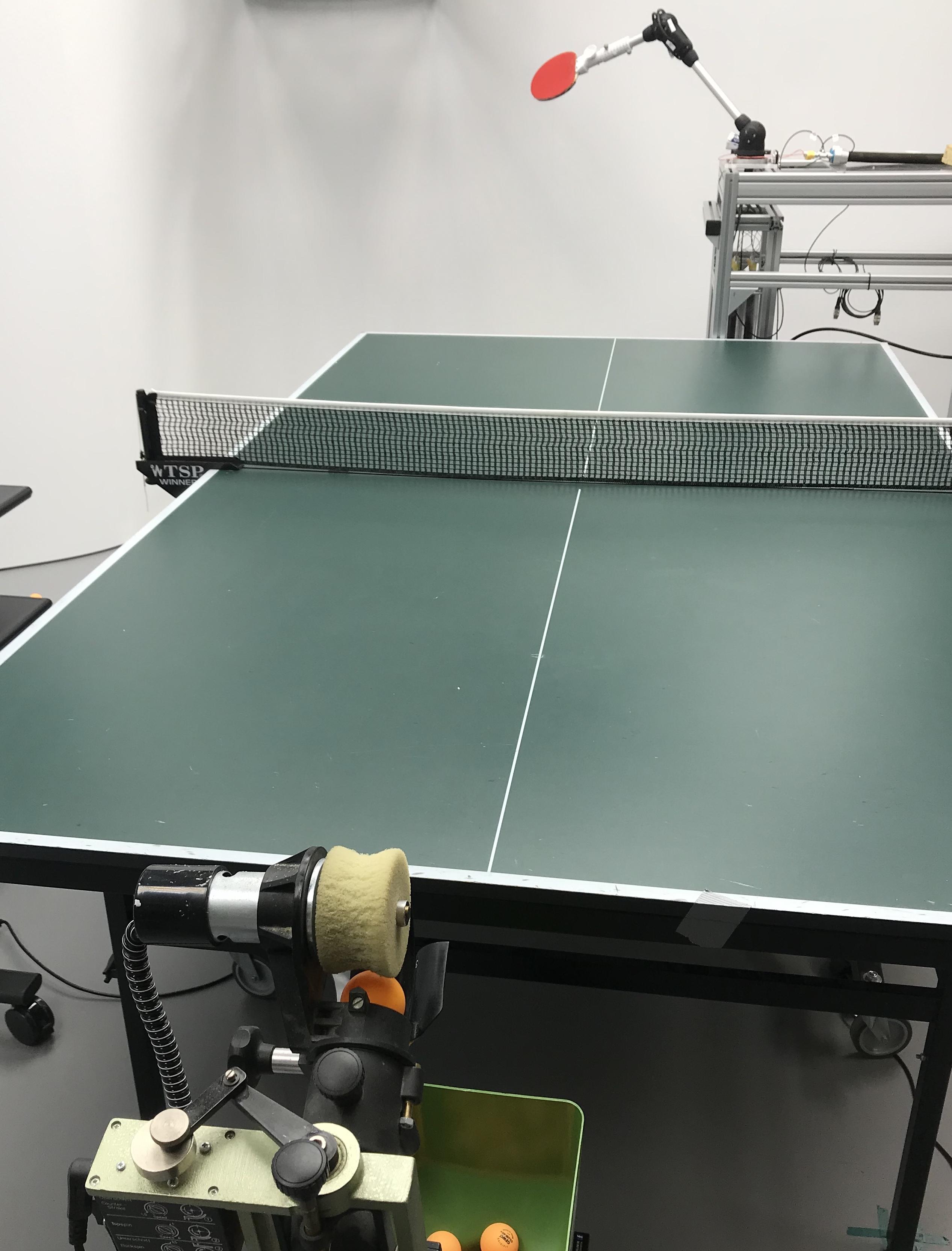
Figure 1: Our setup consists of a four DoF robot arm actuated by pneumatic muscles and a ballgun that launches balls towards the robot arm. The robot successfully learns to return the ball to a desired landing point on the table. The Cartesian positions of the ball are measured by a color-based camera detection system.

In simulation, the agent is allowed to bump into objects, collide with itself, and the actions can act on low-level controls (such as torques or activations to muscles) while being sampled from a stochastic policy. Also, it is possible to employ step-based policies that permit the agent to react in every time step to changes in the state. These changes might produce noisy action sequences as they can vary significantly from one time step to the next (in contrast to episode-based RL where actions are executed in an open-loop fashion and are, hence, usually smooth). All of these points allow the agent to freely explore and learn from failures while interacting for millions of time steps with the environment.

To allow for similar behavior in real world applications of RL, current approaches often constrain robots to slow motion skills such as required for manipulation. For such tasks, simple engineered checks assure robot safety. These checks detect, for instance, collisions with objects (usually based on heuristics) and the robot itself. Safety may be further ensured by limiting joint accelerations and velocities, stopping the robot before it reaches its joint limits, and filtering noisy actions generated by stochastic policies [5, 3]. Also, multiple recent papers point out that robot safety is essential if RL should be reliably employed on real robots [6, 7, 8].

Cautious checks are sufficient for slow movements, e.g., in grasping or lifting objects. However, in tasks such as table tennis, they are not applicable because it is essential to exert explosive motions. In a situation where an incoming ball is supposed to be hit at a point in space far away from the current racket position, the agent needs to rapidly accelerate the racket to gain momentum and reach the hitting point in time. Thus, the amount of accelerations that the robot can generate is proportional to the upper bound of the dexterity it can reach in dynamic tasks. Cautious checks for such problems are disadvantageous because 1) empirically finding parameters for the safety heuristics is substantially harder at faster motions and 2) the safety checks heavily limit the capabilities of robots as they are usually conservatively chosen to avoid damage to the real system reliably.

It is challenging not to limit the performance of dynamic real robotic tasks too much by safety checks while letting the agent freely explore fast motions. For this reason, learning approaches to robot table tennis using anthropomorphic human arm sized systems usually employ techniques such as imitation learning [9], choosing or optimizing from safe demonstrations [10, 11, 12], minimizing acceleration for optimized trajectories [13], distributing torques over all degrees of freedom (DoF) [14] as well as cautious learning control approaches [15].

In [16, 17], it has been shown that systems actuated by pneumatic artificial muscles (PAM) are suitable to execute explosive hitting motions safely. By adjusting the pressure range for each PAM, a fast motion generated by the high forces of the PAMs can be decelerated before a DoF exceeds its allowed joint angle range. Besides, PAM-driven robots are inherently backdrivable, which makes them exceptionally robust. However, such actuators are substantially harder to control than traditional motor-driven systems [18, 19]. For this reason, the predominant use of PAM-driven systems is to slowly handle heavy objects, for disturbance rejection, or as a testbed for control approaches.

In this paper, we show that soft actuation of PAM-driven systems enables RL to be safely applicable to a dynamic task directly on real hardware and, thereby, enable RL to overcome the difficulties of a dynamic task as well as the control issues of soft robots. By enabling RL to explore fast motions directly on the real system, we can leverage the benefits of such complex systems for dynamic tasks (such as high power-to-weight ratio, and storage of energy and release) despite their control issues. In particular, we show that, by using robots actuated by pneumatic artificial muscles (PAM) from [16, 17], the robot learns to return and even smash real table tennis balls using RL from scratch. Rather than avoiding fast motions, we leverage the inherent safety of the robot to favor highly accelerated strikes by maximizing the velocity of the returned ball directly in the reward function. Also, we 1) apply noisy actions sampled from a Gaussian multi-layer perceptron (MLP) policy directly on the low level controls (desired pressures), 2) while running the RL algorithm for millions of time steps on the real hardware, 3) randomly initialize the policy at start and 4) introduce a hybrid sim and real training procedure to circumvent practical issues of long duration training such as collecting, removing and supplying table tennis balls from and to the system. Using this training procedure, the agent learns to return and smash balls without touching any real ball during training.

It is worth mentioning that with our setup, it is possible to learn robot table tennis while adding as little priors on the solution as possible. Neither do we have to add any constraints or regularizers, such as minimal accelerations or energy, nor do we have to use a higher abstraction level like task or joint space but instead learn directly on the low-level controls. Also, we avoid potentially suboptimal models or demonstrations. Models, constraints, and regularizers steer the optimization of the policy to a solution with possibly degenerated performance. Therefore, it is desirable to specify only task-related entities in the reward function and avoid such priors. In this manner, the solution emerges purely from the hardware and the desired behavior defined in the reward function.

To the best of our knowledge, this work is novel in many aspects: First, it demonstrates the first results in learning the challenging task of playing table tennis with muscular robots. Second, this paper pioneers learning smash hitting motions on real robots rather than only returning balls to the opponent’s side of the table. Third, this work pioneers the safe application of model-free RL on safety-critical dynamic tasks. Fourth, we present the first approach to robot table tennis, where the training does not involve real balls.

The remaining of the paper is divide as follows: In Section II, we introduce the task and reward functions used to learn to return and smash as well as the hybrid sim and real training procedure (HYSR). The return and smash experiment are described in detail in Section III. We summarize the contributions and discuss the results in Section IV.

II Training of Muscular Robot Table Tennis

Learning dynamic tasks using muscular robots allows the RL algorithm to run on real systems similarly to when applied to simulated robots. In return, RL helps to overcome the inherent control difficulties PAM-driven systems and leverage its beneficial properties such as the powerful actuation to learn to return and smash real table tennis balls to desired landing points. To illustrate the details of this symbiosis, we introduce the task setup, the dense rewards used for the experiments, as well as the hybrid sim and real training (HYSR) that enables practical learning of these tasks.

Variability in Recorded Ball Trajectories

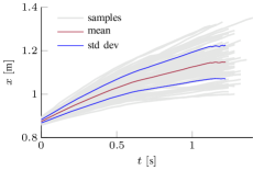
(a)

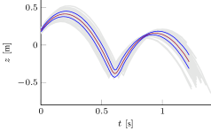
(b)

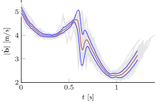
(c)

(d)

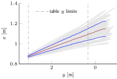
(e)

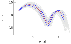
(f)

Figure 2: Variability of the recorded ball trajectory dataset $\mathcal{D}^{\text{rec}}$. A ball launcher with fixed settings launches table tennis balls towards the robot. A color-based camera vision system [20] provided the position of the ball at $180\text{\,}\mathrm{Hz}$. Variability is quantified by the sample mean and sample variance with respect to time a) to c) and along the long side of the table ($y$ coordinate) d) to f). The $x$ coordinate aligns with the shorter edge of the table and $z$ coordinate links to the normal of the table plane. Although the settings of the ball launcher are constant, the ball varies substantially: 1) variability increases throughout the trajectory, especially after the bounce, 2) the first bounce on the table (incoming ball) varies around $50\text{\,}\mathrm{cm}$ along $y$-coordinate (subfigure e)). 3) the agent has to handle deviation of around $40\text{\,}\mathrm{cm}$ along the $x$-axis and $\sim$$50\text{\,}\mathrm{cm}$ along the $z$-axis when the ball is in reach for the hit. 4) the variability with respect to time and the $y$-axis increases over time, which means that the agent cannot simply learn to start the hit after a particular fixed duration. Additionally, the agent needs to learn to adjust the amount of energy it transfers to each ball as the ball velocity also varies at the end of the table.

II-A Muscular Robot Table Tennis Task Setup

The considered table tennis task consists of returning an incoming ball with the racket attached to the robot arm to a desired landing point on the table $\bm{\mathrm{b}}^{\text{des}}\in\mathbb{R}^{2}$. We denote the ball trajectory $\bm{\mathrm{\tau}}^{\text{b}}=[\bm{\mathrm{s}}^{\text{b}}_{t}]_{t=0}^{T}$ consisting of a series of ball states $\bm{\mathrm{s}}^{\text{b}}_{t}=[\bm{\mathrm{b}}_{t},\dot{\bm{\mathrm{b}}}_{t}]$ that themselves contain the current ball position $\bm{\mathrm{b}}_{t}\in\mathbb{R}^{3}$ and velocity $\dot{\bm{\mathrm{b}}}_{t}\in\mathbb{R}^{3}$. In a successful stroke, the robot hits the ball at time $t_{\text{h}}$ and position $\bm{\mathrm{b}}^{\text{h}}$ such that the ball lands on the table plane at position $\bm{\mathrm{b}}^{\text{land}}$ at time $t_{\text{land}}$. The ball crosses the plane aligned with the net on the incoming and outgoing ball trajectory at position $\bm{\mathrm{b}}^{\text{n}_{\text{in}}}\in\mathbb{R}^{2}$ at time $t_{\text{n}_{\text{in}}}$ and $\bm{\mathrm{b}}^{\text{n}_{\text{out}}}\in\mathbb{R}^{2}$ at time $t_{\text{n}_{\text{out}}}$ if the robot successfully returns the ball.

Table tennis falls into the general class of dynamic tasks such as baseball [21], tennis or hockey [22]. Dynamic tasks represent a class of problems that are relatively easy to solve for humans but hard for robots. The features of dynamic tasks are 1) quick reaction times as adapting to changes in the environment (such as moving balls) must happen fast, 2) precise motions because objects are supposed to reach some goal state (e.g. desired landing position on the table) and 3) fast and highly accelerated motions. The latter point is particularly important for two reasons: First, a successful strategy can incorporate fast strikes such as a table tennis smash. Second, if the desired hitting position of the ball is far from the current racket position, highly accelerated motions help to reach this point in time. Thus, the maximum acceleration the system is capable of generating represents the upper limit to the dexterity the agent can develop at such tasks. The class of dynamic problems differs from manipulation, where the task itself can be richer than a dynamic task in the sense that the objects and setting can vary largely. Unlike in dynamic tasks, however, slow motions and small accelerations are usually sufficient.

Safely generating high accelerations is harder with anthropomorphic robots than with parallel [23] or Cartesian systems [24]. Low inertia and force transmission without cables ease the control of these systems, making high acceleration and estimating potentially dangerous motions feasible. Our work, in contrast, investigates table tennis with anthropomorphic robots. Damages on such systems can occur by breaking cables due to fast-changing control commands or exceeding joint limits when the system cannot stop in time. Learning the solution to the task while assuring robot safety makes anthropomorphic table tennis especially challenging.

Pneumatic artificial muscles (PAMs) are a particularly useful actuation system for anthropomorphic robots when applied to dynamic tasks. This actuators contract if the air pressure inside increases, hence at least two PAMs act antagonistically on one degree of freedom (DoF) as a single PAM can only pull and not push. In this paper, we leverage the PAM-driven robot arm developed in [16, 17] which has four DoFs actuated by eight PAMs. Such robots are capable of generating high accelerations due to a high power-to-weight ratio. At the same time, adjusting the allowed pressures ranges prevents exceeding joint limits despite fast motions. We use this property in III-A and III-B to let the RL agent freely explore fast motions without any further safety considerations. Another benefit of PAM-driven systems is the inherent robustness resulting from passive compliance. This property helps reducing damage at impact due to shock absorption [25] as well as the adjustable stiffness via co-contracting the PAMs in an antagonistic pair. In this paper, we leverage this robustness to apply stochastic policies directly on the desired pressures, which are the low-level actions in this system (see Figure 4).

These numerous beneficial properties come at the cost of control challenges. PAMs are highly non-linear systems that change their dynamics with temperature as well as wear and are prone to hysteresis effects. Thus, modeling such systems for better control is challenging [18, 19]. PAMs are, for this reason, predominately used as a testbed for control algorithms rather than dynamic tasks. In this work, we show that it is possible to satisfy the precision demands of the table tennis task despite the control difficulties of PAM-driven systems by using RL (see III-A and III-B).

II-B Dense Reward Functions For Returning and Smashing

We formulate the learning problem as an episodic Markov Decision Process (MDP)

$$\mathcal{M}=(\mathcal{S},\mathcal{A},r,\mathcal{P},p_{0},\gamma)\,$$ (1)

where $\mathcal{S}$ is the state space, $\mathcal{A}$ is the action space, $r:\mathcal{S}\times\mathcal{A}\mapsto\mathbb{R}$ is the immediate reward function, $\mathcal{P}:\mathcal{S}\times\mathcal{A}\mapsto\mathcal{S}$ is the transition probability or dynamics, $p_{0}$ is the initial state distribution and $\gamma\in[0,1]$ the discount factor. The goal in RL is to find a policy $\pi:\mathcal{S}\mapsto\mathcal{A}$ that maximizes the expected return $J=\mathbb{E}_{\bm{\mathrm{\tau}}}\sum_{t=0}^{T}\gamma^{t}r(\bm{\mathrm{s}}_{t},\bm{\mathrm{a}}_{t})$ where $\bm{\mathrm{\tau}}=(\bm{\mathrm{s}}_{0},\bm{\mathrm{a}}_{0},\bm{\mathrm{s}}_{1},\bm{\mathrm{a}}_{1},\ldots,\bm{\mathrm{s}}_{T})$ is the state action trajectory, $\bm{\mathrm{s}}_{0}\sim p_{0}$, $\bm{\mathrm{a}}_{t}\sim\pi(\bm{\mathrm{s}}_{t})$ and $\bm{\mathrm{s}}_{t+1}=\mathcal{P}(\bm{\mathrm{s}}_{t},\bm{\mathrm{a}}_{t})$.

The state $\bm{\mathrm{s}}=[\bm{\mathrm{s}}^{\text{b}},\bm{\mathrm{s}}^{\text{r}}]$ we use here is composed of the ball state $\bm{\mathrm{s}}^{\text{b}}$ and the robot state $\bm{\mathrm{s}}^{\text{r}}$. The robot state $\bm{\mathrm{s}}^{\text{r}}=[\bm{\mathrm{q}},\dot{\bm{\mathrm{q}}},\bm{\mathrm{p}}]$ consists of the joint angles $\bm{\mathrm{q}}\in\mathbb{R}^{4}$, joint angle velocities $\dot{\bm{\mathrm{q}}}\in\mathbb{R}^{4}$ and air pressures in each PAM $\bm{\mathrm{p}}\in\mathbb{R}^{8}$. The ball state $\bm{\mathrm{s}}^{\text{b}}=[\bm{\mathrm{b}},\dot{\bm{\mathrm{b}}}]$ has been already defined in II-A. The system we utilize here actuates each DoF with two PAMs. The actions $\bm{\mathrm{a}}$ are the change in desired pressures in each PAM $\Delta\bm{\mathrm{p}}^{\text{des}}\in\mathbb{R}^{8}$.

In practice, the true Markovian state $\bm{\mathrm{s}}$ is not accessible in experiments with real robots. Especially for PAM driven systems, the Markov state composition is unclear [19] leading to a Partially Observable MDP (POMDP) which assumes to receive observations $\bm{\mathrm{o}}$ of the true state $\bm{\mathrm{s}}$. For the sake of clarity, we continue using $\bm{\mathrm{s}}$ instead of $\bm{\mathrm{o}}$ notation. The immediate reward function $r(\bm{\mathrm{s}}_{t},\bm{\mathrm{a}}_{t})$ defines the goal of the task. The task of returning an incoming ball to a desired landing point can be divided into two stages: 1) manage to hit or touch the ball and 2) fine-tune the impact of the ball with the racket such that it flies in a desired manner. As the landing location of the ball changes only in case the robot manages to hit the ball, we introduce a conditional reward function

$$r=\begin{cases}r^{\text{tt}}\,&\text{racket touches the ball}\\ r^{\text{hit}}&\text{otherwise}\,,\end{cases}$$ (2)

where $r^{\text{tt}}$ is the table tennis reward

$$r^{\text{tt}}=\begin{cases}1-c||\bm{\mathrm{b}}^{\text{land}}-\bm{\mathrm{b}}^{\text{des}}||^{\frac{3}{4}}&\text{return task}\\ (1-c||\bm{\mathrm{b}}^{\text{land}}-\bm{\mathrm{b}}^{\text{des}}||^{\frac{3}{4}})\max_{t>t_{\text{h}}}||\dot{\bm{\mathrm{b}}}_{t}||&\text{smash task}\end{cases}$$ (3)

that evaluates the stroke depending on the ball trajectory after the impact of the ball and racket. In particular, it considers the distance of the actual landing point $\bm{\mathrm{b}}^{\text{land}}$ to the desired landing point $\bm{\mathrm{b}}^{\text{des}}$ for the return task (see III-A). The normalization constant $c=||\bm{\mathrm{\tau}}^{\text{r}}_{0}-\bm{\mathrm{b}}^{\text{des}}||^{-1}$ is chosen such that $r^{\text{tt}}$ is usually within the range $[0,1]$ where $\bm{\mathrm{\tau}}^{\text{r}}_{0}$ is the initial racket position. We also cap the table tennis reward $r^{\text{tt}}=\max(r^{\text{tt}},-0.2)$ in order to avoid too negative rewards in case the ball flies into a random direction with high velocity as happens if hit by an edge of the racket. We also introduce an exponent to the components of $r^{\text{tt}}$ to cause the values of the rewards to be more different closer to the optimal value. We found the exponent $\nicefrac{{3}}{{4}}$ to empirically work well. For the smashing task, the agent is supposed to maximize the ball velocity $\dot{\bm{\mathrm{b}}}$ simultaneously. The product between these two goals forces the agent to be precise and play fast balls as $r^{\text{tt}}$ is small overall if a single component has a low value. The hitting reward

$$r^{\text{hit}}=-\min_{t}||\bm{\mathrm{\tau}}^{\text{b}}_{t}-\bm{\mathrm{\tau}}^{\text{r}}_{t}||\,$$ (4)

is a dense reward function representing the minimal Euclidean distance in time between the ball trajectory $\bm{\mathrm{\tau}}^{\text{b}}$ and Cartesian racket trajectory $\bm{\mathrm{\tau}}^{\text{r}}$ where $\bm{\mathrm{\tau}}^{\text{r}}_{t}=\bm{\mathrm{x}}^{\text{r}}_{t}=\mathcal{T}(\bm{\mathrm{q}}_{t})\in\mathbb{R}^{3}$ using the forward kinematics function $\mathcal{T}(\cdot)$, the Cartesian racket position $\bm{\mathrm{x}}^{\text{r}}_{t}$ and ignoring the racket orientation. This reward function encourages the agent to get closer to the ball and finally hit it by providing feedback about how close it missed the racket.

Note that we do not incorporate any safety precautions such as state constraints like joint ranges, minimal accelerations $||\ddot{\bm{\mathrm{q}}}_{t}||$ or change in actions $||\bm{\mathrm{a}}_{t}-\bm{\mathrm{a}}_{t-1}||$ into the reward function. On the contrary, we add a term that favors faster hitting motions. By doing so, we let the solution emerge purely from the hardware and the reward function that - in our case - incorporates only task-related terms.

II-C HYSR: Hybrid Sim and Real Training

Running experiments with real robots and real objects for millions of time steps is a tedious practical effort. For instance, learning robot table tennis using model-free RL involves launching balls automatically, removing them from the scene after the stroke, and returning them to the ball reservoir. Automating this pipeline takes a substantial amount of work. Hence, we considered training with simulated balls. Training in simulation, however, can be problematic: Simulated balls might differ too much from the real ball so that the learned policy might not be useful when playing with real balls. Additionally, the lack of good models of PAM-driven systems [18, 19] renders simulating the real robot infeasible.

For this reason, we introduce a hybrid sim and real training (HYSR) where the key idea is to use real data as much as possible and simulations wherever necessary. Specifically, actions $\bm{\mathrm{a}}$ sampled from the policy $\pi$ are applied to the real robot, but the ball exists only in simulation during training. In simulation, we replay a single ball trajectory per episode sampled uniformly from a prerecorded data set $\mathcal{D}^{\text{rec}}=[\bm{\mathrm{\tau}}^{\text{rec,$i$}}]^{N^{\text{rec}}}_{i=0}$. Within the recorded data set $\mathcal{D}^{\text{rec}}$ the $i$-th trajectory consist of a sequence of ball states $\bm{\mathrm{\tau}}^{\text{rec,$i$}}_{t}=\bm{\mathrm{s}}^{\text{rec}}_{t}$.

The real robot is copied to the simulation by overwriting the simulated with the real robot state $\bm{\mathrm{s}}^{\text{r}}$ in every time step. In this manner, the real robot moves in simulation in the same way as in reality. In this manner, the simulation and the real scenery stay identical (the only difference being that the ball has been launched before training) until contact of the ball with the racket. At this point, it is impossible to predict the subsequent ball trajectory from $\mathcal{D}^{\text{rec}}$. For this reason, we start simulating the ball after the impact, which allows us to calculate the landing point of the ball $\bm{\mathrm{b}}^{\text{land}}$ more reliably as we simulate at the latest possible point.

Algorithm 1 HYSR: Hybrid Sim and Real Training

1:  while max_timesteps not reached do

2:     $i\sim\text{uniform}(0,N^{\text{rec}})$

3:     $\bm{\mathrm{\tau}}^{\text{rec}}\leftarrow\mathcal{D}^{\text{rec}}_{i}$

4:     $t\leftarrow 0$

5:     racketTouched$\leftarrow$false

6:     while episode end not reached do

7:        $\bm{\mathrm{s}}^{\text{r}}_{t}\leftarrow$readSensors()

8:        if racketTouched then

9:           $\bm{\mathrm{s}}^{\text{sim}}_{t}\leftarrow\text{sim}(\bm{\mathrm{s}}^{\text{sim}}_{t-1})$

10:           $\bm{\mathrm{s}}_{t}\leftarrow[\bm{\mathrm{s}}^{\text{r}}_{t},\bm{\mathrm{s}}^{\text{sim}}_{t}]$

11:        else

12:           $\bm{\mathrm{s}}^{\text{rec}}_{t}\leftarrow\bm{\mathrm{\tau}}^{\text{rec}}_{t}$

13:           $\bm{\mathrm{s}}_{t}\leftarrow[\bm{\mathrm{s}}^{\text{r}}_{t},\bm{\mathrm{s}}^{\text{rec}}_{t}]$

14:        end if

15:        if $\textrm{racketTouchesBall}(\bm{\mathrm{s}}_{t})$ then

16:           racketTouched$\leftarrow$ true

17:        end if

18:        $\bm{\mathrm{a}}_{t}\sim\pi(\bm{\mathrm{s}}_{t})$

19:        $t\leftarrow t+1$

20:     end while

21:     update $\pi$ using PPO

22:  end while

Essential for sufficiently accurate transfer from simulated to the real ball within HYSR is the rebound model of the ball with the racket. We found the rebound model from [26] to work well after optimizing its parameters empirically. The model

$$\dot{\bm{\mathrm{b}}}_{\text{out}}-\dot{\bm{\mathrm{x}}}^{\text{r}}_{t_{\text{h}}||}=\epsilon_{\text{R}}(-\dot{\bm{\mathrm{b}}}_{\text{in}}+\dot{\bm{\mathrm{x}}}^{\text{r}}_{t_{\text{h}}||})$$ (5)

calculates the outgoing velocity of the ball $\dot{\bm{\mathrm{b}}}_{\text{out}}$ from the ball velocity $\dot{\bm{\mathrm{b}}}_{\text{in}}$ before impact, the racket speed $\dot{\bm{\mathrm{x}}}^{\text{r}}_{t_{\text{h}}||}$ at impact (all measured along the racket normal) and the restitution coefficient of the racket $\epsilon_{\text{R}}$. Note that this model assumes no spin. Algorithm 1 summarizes a single episode of the training procedure.

It is important to mention that, although the settings of the ball launcher have been kept fixed, the $N^{\text{rec}}{}=100$ recorded ball trajectories in $\mathcal{D}^{\text{rec}}$ largely vary as can be seen in Figure 2. Variability arises through the noise in the color-based vision system that automatically detects balls and returns their Cartesian position. Another reason is that the ball launcher adds little noise to each ball, accumulating to more significant deviations the farther the ball flies.

HYSR allows us to leverage the simulation conveniently to estimate the landing position $\bm{\mathrm{b}}^{\text{land}}$ and other context entities such as distances or boolean contact indicators that are important for the reward (see Equation (4) and Equation (3)). Besides, we avoid collecting and launching real balls. Note that this way of training can serve as an entry point for sim2real techniques such as domain randomization or curriculum learning. For instance, the progress of the training could be used to update the ball’s initial state $\bm{\mathrm{s}}^{\text{b}}_{0}$, or the ball trajectory $\bm{\mathrm{\tau}}^{\text{b}}$ can be perturbed.

III Experiments and Evaluations

Learning Curves of Return and Smash Experiments

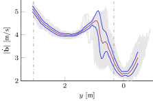
(a) smash

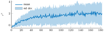
(b) return

Figure 3: Sample mean and standard deviation of the rewards of each episode for the a) smash and b) return task from Section III-A and Section III-B. The policies for both experiments were updated 183 times. The number of episodes differs for each experiment as we define the end of the training by the number of time steps (1.5 million for both experiments at $10\text{\,}\mathrm{ms}$), but the actual episode length varies. The return task required 15676 and the smash task 15161 strokes or episodes. Each episode takes approximately $1\text{\,}\mathrm{s}$ with additional initialization of the robot ($2$ to $4\text{\,}\mathrm{s}$, see Figure 6a) The total moving time is $14\text{\,}\mathrm{h}$ and $10\text{\,}\mathrm{min}$ for the return task and $14\text{\,}\mathrm{h}$ and $18\text{\,}\mathrm{min}$ for the smash experiment.

The key contributions of this paper are to 1) enable RL to explore fast motions of soft robots without safety precautions, by doing so, 2) learn a difficult dynamic task using RL with a complex real system. To show 2), we learn to return and smash a table tennis ball with a PAM-driven robot arm using the HYSR training described in Section II-C and the reward functions discussed in Section II-B. We highlight 1) by quantifying the robustness of the system during the training. In particular, we illustrate the speed of the returned ball and depict the noisy actions on the low-level controls of the real system due to the application of a stochastic policy. Results are best seen in the supplemental videos at muscularTT.embodied.ml.

III-A Learning to Return

Returning table tennis balls with PAM-driven systems is a challenging problem due to PAMs being hard to model and control [18, 19] and table tennis requiring precise control of the racket at impact with the ball. In this task, the robot’s task is to return balls to a desired landing position $\bm{\mathrm{b}}^{\text{des}}$ (see Figure 7) on the opposite side of the table shot by a ball launcher as shown in Figure 1 and described in Section II-A. We demonstrate that by enabling RL to explore freely at fast paces, the agent can learn this task well.

We let the robot train for $1.5$ million time-steps using a stochastic policy. The policy has been randomly initialized and the actions are changes in target pressures $\Delta\bm{\mathrm{p}}^{\text{des}}$. One strike corresponds to one episode. At the end of each episode, the agent receives a reward according to the dense return reward function from Equation (3). We use PPO [27] as a backbone RL algorithm. In particular, we leverage the ppo2 implementation of PPO from OpenAI baseline [28]. Table I lists the hyperparameters used for this experiment.

After training, the final policy has been evaluated with real balls. The agent hits 96% and returns 77% of the 107 real balls shot by the ball launcher, as indicated in Table II. Figure 7 illustrates that the landing points spread in a circle around the desired landing point. This circle overlaps with the opponent’s side but is not fully contained by it. Thus, the return rate to the table would have been higher if $\bm{\mathrm{b}}^{\text{des}}$ would be moved towards the center of the table half.

Interestingly, the agent did not only learn to intercept the ball but also to prepare for the hit, as can be seen in Figure 6. These two stages are part of the four stages of a table tennis game introduced in [29] and recorded from play in [26]. This behavior emerged, although the goal was only to return the ball to a desired landing point. Specifying the same behavior within the classical pipeline of 1) planning a reference trajectory and 2) tracking with an existing (model-based) controller appears to be more difficult: Such approaches have the disadvantage of relying on human expert knowledge, which is likely to lead to non-optimal solutions considering the challenges of the control problem being solved. Hence, this work represents a type of end-to-end approach to dynamic tasks where we learn a mapping from sensor information to low-level controls directly. This kind of approaches are only possible if the hardware is sufficiently robust.

Noisy Actions of Stochastic Policy Applied Directly to Low Level Controls

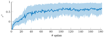
(a)

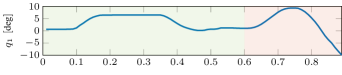
(b)

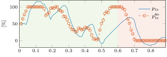
(c)

Figure 4: Noisy actions due to sampling of a stochastic policy in every time step exemplified on the first DoF with both antagonistic PAMs $p_{1\text{a}}$ and $p_{1\text{b}}$ of one episode. The pressures are normalized between $[0\%\ldots 100\%]$ to indicate that pressure ranges which map to $[$0\text{\,}\mathrm{bar}$\ldots$3\text{\,}\mathrm{bar}$]$. The low-level controls of the system are the desired pressures $p^{\text{des}}$ which are set by the RL policy. $p_{1\text{a}}$ and $p_{1\text{b}}$ switch along the whole pressure range multiple times during the episode. The impact with the ball happens at $t=$0.9\text{\,}\mathrm{s}$$. At $t=$0.6\text{\,}\mathrm{s}$$ the agent switches the pressures from minimum to maximum and vice versa to hit the ball. The green and red background color indicate the two distinct phases of preparation and hit from Figure 6. Applying such action sequences to the low level controls of traditional robots of similar dimensions (e.g. link lengths) likely breaks the system. Figure 8 visualizes this return and a smash motion in more detail.

Histogram of Maximal Speeds of Returned Balls

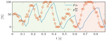
Figure 5: Histograms depicting the speeds of the balls for the return and smash experiment. Considered are the maximum velocities after impact with the racket. The final policy of each experiment generated the data for the particular histogram. One can see that the speeds significantly increase for the smashing experiment.

Table I: Hyperparameters used for RL experiments

hyperparameter	value
algorithm	ppo2
network	mlp
num_layers	1
num_hidden	512
activation	tanh
nsteps	4096
ent_coef	0.001
learning_rate	lambda f:1e-3*f
vf_coefs	0.66023
max_grad_norm	0.05
gamma	0.9999
lam	0.98438
nminibatches	8
noptepochs	32
cliprange	0.4

Visualization of Learned Two Stage Hitting Motion

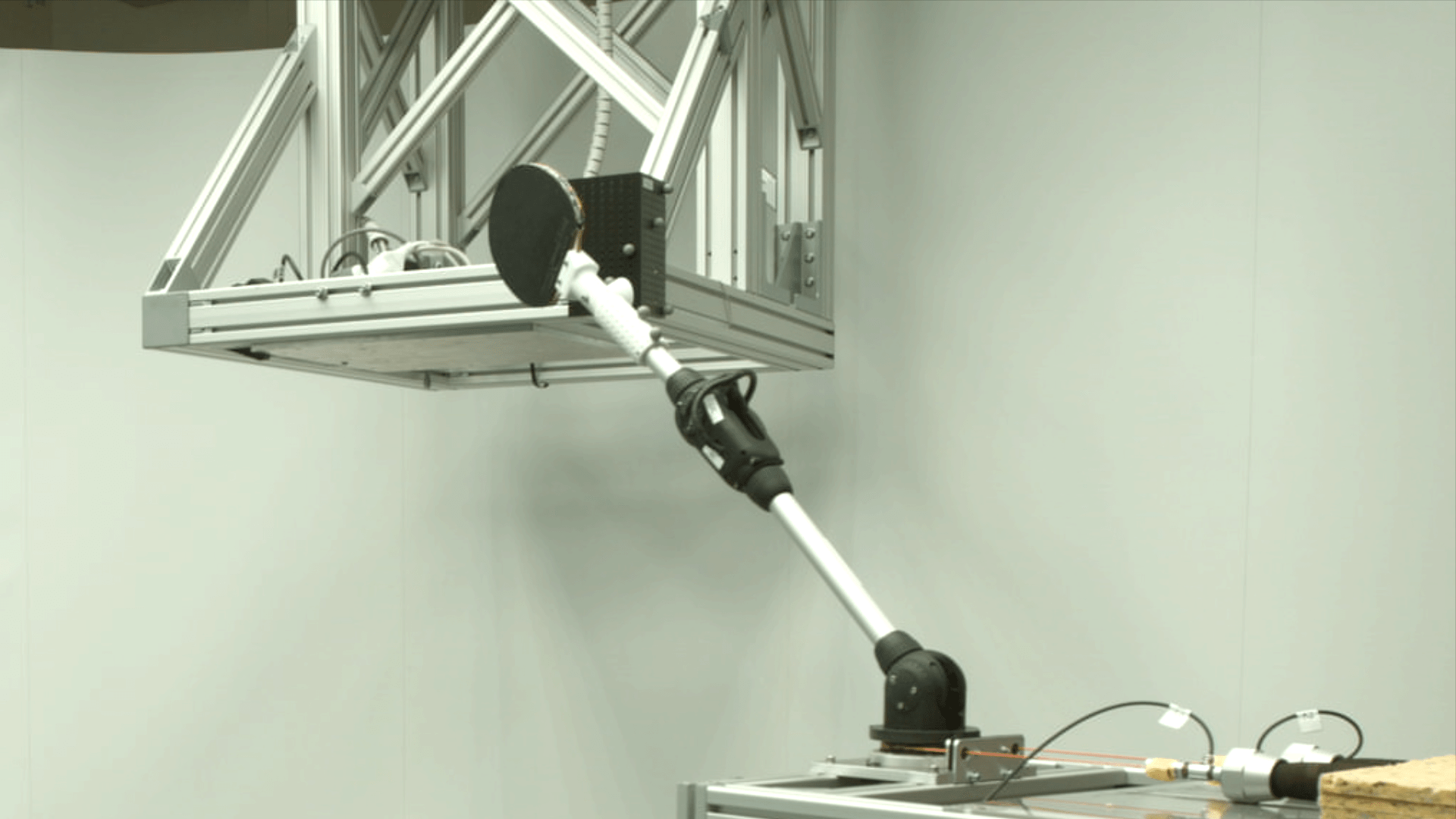
(a) Initial posture

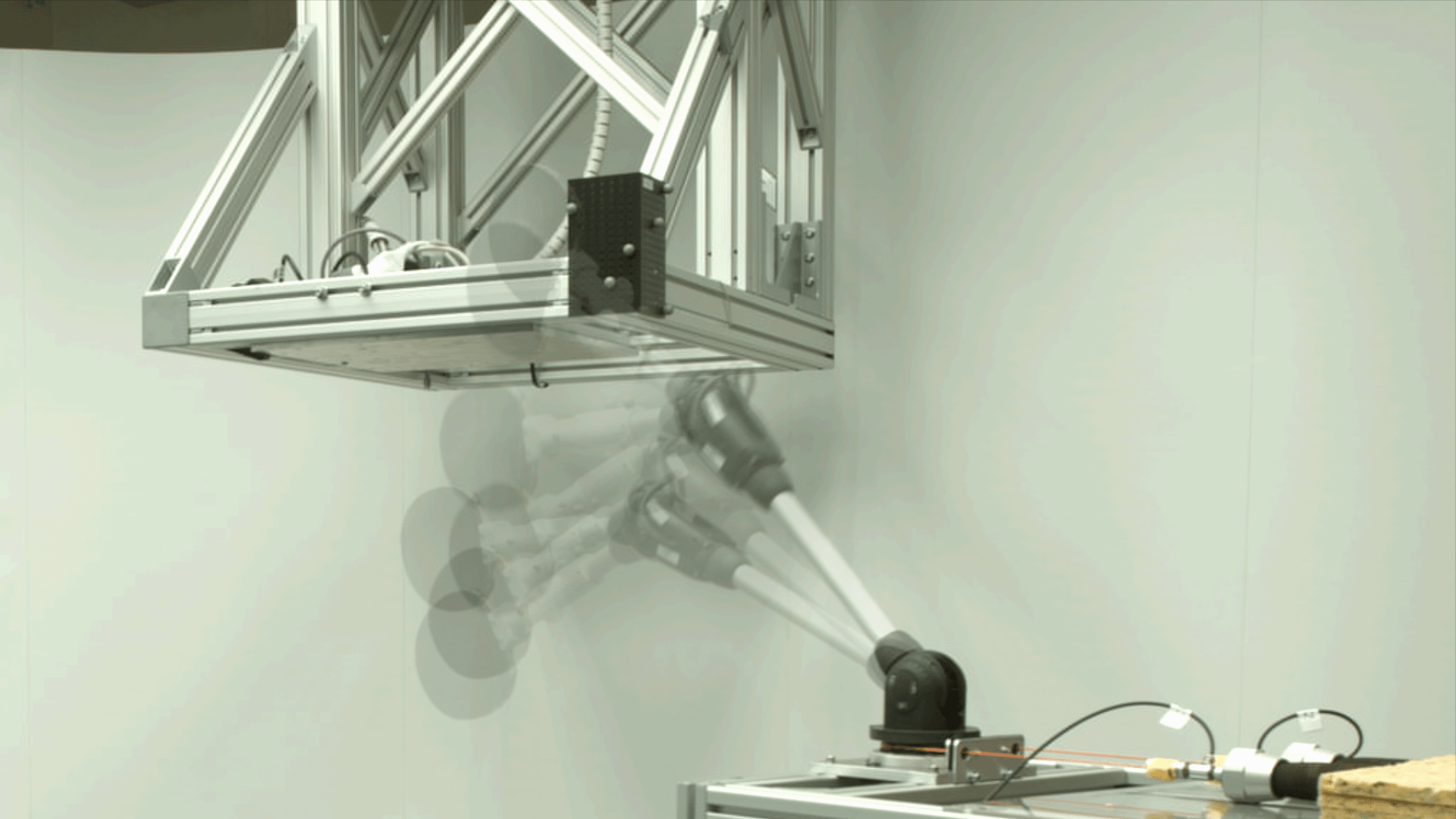
(b) Preparing for hit

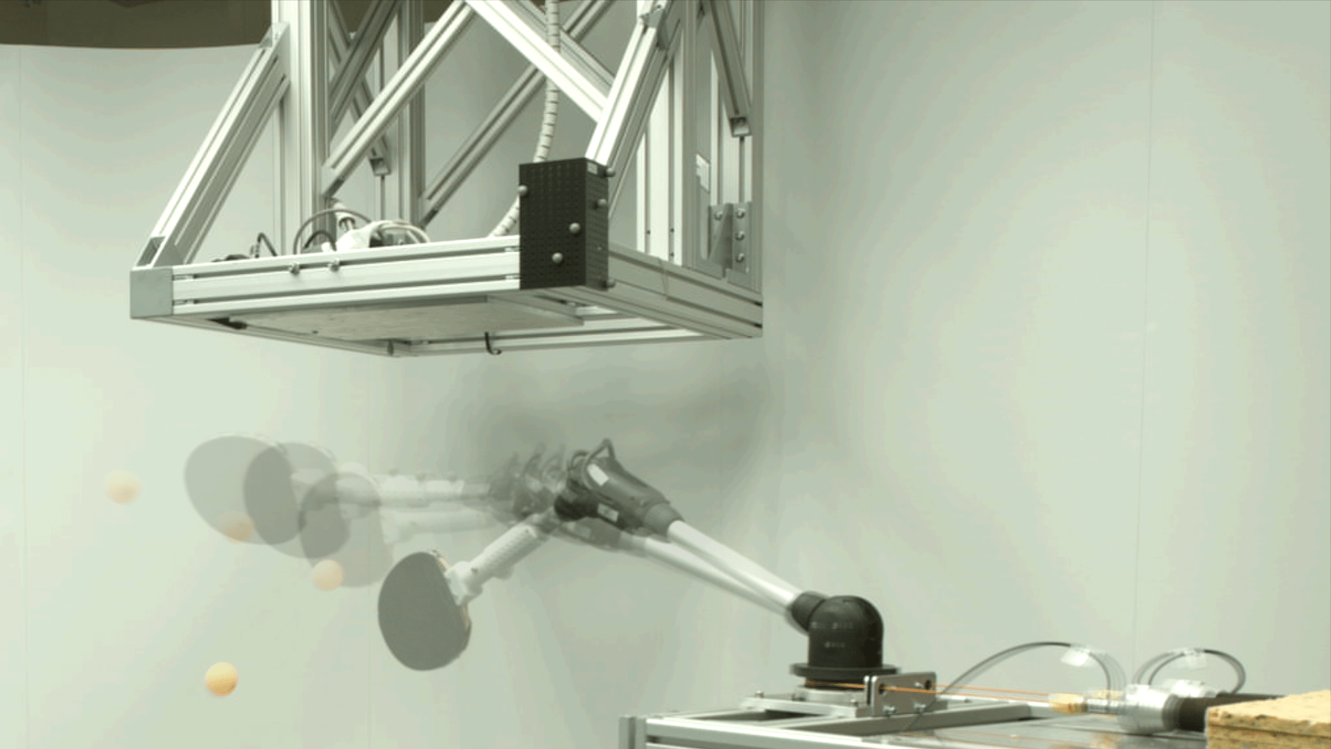
(c) Actual hit

Figure 6: Images extracted from a video showing the learned hitting motion of the return experiment. After an episode, the robot initializes to an initial position shown in a), which takes $2\text{\,}\mathrm{s}$ to $4\text{\,}\mathrm{s}$. The agent automatically learned two distinctive hitting stages consisting of b) preparing for a hit and c) the actual hit.

III-B Learning to Smash

In table tennis, smashing is a means of maximizing the ball’s velocity, such that the opponent has a hard time returning it. The motion needs to be very fast and, at the same time, precise enough to return the ball to the opponent’s side. Smashing is harder to learn than just returning balls as imprecise motions might lead to the ball not being returned on the table entirely. Here we show that, by using soft robots, we can learn this skill using RL only by defining a reward function that maximizes the ball speed and minimizes the distance to the desired landing point (Equation (3)) concurrently. Rather than taking safety into account algorithmically, we - on the contrary - favor aggressive and explosive motions.

We chose to repeat the experiment from Section III-A with the same hyperparameters as in Section III-A but updated the reward function with the speed bonus from Equation (3). The learning curve is depicted in Figure 3. In comparison with the learning curve from Section III-A, the smashing task is harder to learn for the agent. The standard deviation of the reward for the smash experiment is higher than in the return task. Also, the precision of the returned balls is lower in the smash experiment, as shown in Figure 7.

Figure 5 shows histograms of the maximum ball velocities after the hit for reward function with and without speed bonus. The ball speed increases when the reward contains a speed bonus. For the return task, the robot returns balls at $5\text{\,}\mathrm{m}\text{\,}{\mathrm{s}}^{-1}$ on average, whereas in the smash experiment, this number increases to $12\text{\,}\mathrm{m}\text{\,}{\mathrm{s}}^{-1}$. Note that [30] considers balls faster than $10\text{\,}\mathrm{m}\text{\,}{\mathrm{s}}^{-1}$ to be smashes in human play.

The higher return speed comes at a cost: The return and hitting rates indicated in Table II show that the faster the hit, the robot returns the ball less precisely. Hence, the more energy is transferred to the ball, the higher the chance of failing.

Table II: Return and hitting rates of return (107 trails) and smash (128 trails) experiments

task	hitting rate	rate of returning to opponents side
return	0.96	0.75
smash	0.77	0.29

Precision of Returned Balls

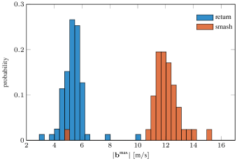
Figure 7: Landing positions of the returned balls for the return as well as for the smash experiment from Section III-A and Section III-B. The landing points of the smash experiment are further apart from the desired landing point compared to the return experiment as can be seen by the fitted Gaussian distributions. The mean of this distribution for the return experiment coincides with the desired landing point $\bm{\mathrm{b}}^{\text{des}}$ but is shifted for the smash experiment. At the same time the smashed balls are faster, hence, corresponding to a more aggressive but risky game play strategy. At such speeds, small error in the racket orientation leads to bigger deviations in landing point.

III-C Robustness

The robustness of the PAM-driven robot arm enables the RL algorithm to explore fast motions while executing a stochastic policy directly on the low-level controls. We quantify the robustness of this PAM-driven system in multiple manners.

First, the sheer number of running a real system for 1.5 million training time-steps stresses that soft robots are indeed robust. 1.5 million time steps at $100\text{\,}\mathrm{Hz}$ are equivalent to $4\text{\,}\mathrm{h}$ and $16\text{\,}\mathrm{min}$ of actual training time. Also, the robot initializes after each episode, which takes further $2$ to $4\text{\,}\mathrm{s}$ per episode. In total, we train the return task for $14\text{\,}\mathrm{h}$ and $18\text{\,}\mathrm{min}$ and the smash task for $14\text{\,}\mathrm{h}$ and $10\text{\,}\mathrm{min}$. Within these durations, the policies of both experiments are updated 183 times, and we perform 15676 (return) and 15161 (smash) strokes, each corresponding to one episode. Note that the training stopped because the algorithm converged and not due to hardware issues.

Second, each episode is carried out by sampling actions from a Gaussian multi-layer perceptron (MLP) at every time-step. For this reason, the signals are noisy and can vary substantially with each time step. Figure 4 depicts the actions $\Delta\bm{\mathrm{p}}^{\text{des}}_{1\text{a}}$ and $\Delta\bm{\mathrm{p}}^{\text{des}}_{1\text{b}}$ of the first DoF and the measured pressures $p_{1\text{a}}$ and $p_{1\text{b}}$ in percent of the allowed pressure ranges alongside with the corresponding joint angle $q_{1}$. The hit of the ball happens at $0.9\text{\,}\mathrm{s}$. The agent learned to switch the actions from minimum to maximum pressure and vice versa around $t=$0.6\text{\,}\mathrm{s}$$ right before the hit. In the preparation phase (see Figure 6a) before the hit (indicated by the green background color in 4), the agent used the whole pressure range to bring the robot into a beneficial initial state for the hit. Applying such signals to the low-level controls of a traditional motor-driven system with the same dimensions as our robot arm presumably causes damage or at least severe wear.

Third, in both experiments, we learn from scratch, where the initial policy receives random weights. Nevertheless, the motions during training did not exceed the joint limits because the allowed pressure ranges have been set such that one of the muscles in the antagonistic pair is stretched close to the respective joint limit [16, 17]. In this manner, the robot can train without human supervision. To achieve safety for dynamic motions on traditional robotic systems, a filter on the actions would be required, such as in [5]. However, there are multiple downsides to this approach: 1) Adding a filter makes the state non-Markovian if the internal filter state is not part of the RL state, which would, in turn, increase the RL state’s dimensions. 2) Tuning the filter can be tedious: On the one hand, setting the parameters too conservatively leads to slower motions, although the task requires fast motions. On the other hand, too optimistic parameters might damage the robot for some configurations. 3) Filtering the stochastic output of the policy counteracts its intended use.

IV Conclusion

Accurately returning and smashing table tennis balls to a desired landing point with anthropomorphic robots requires the execution of precise and fast motions. Exploration at fast speeds is highly desirable for improving accuracy but might damage the robot, e.g., exceeding joint limits. The synergy between soft robots and Reinforcement Learning for dynamic tasks resolves this dilemma. The robustness of soft actuation allows RL to act like in simulation and, vice versa, RL helps to overcome the difficulties of the table tennis tasks and the control problems of soft robots. A particularly interesting finding is that in our experiments, it was neither necessary to take safety into account in the algorithm nor was any model or demonstration needed. On the contrary: We even encouraged returning the ball with high speed by an additional term in the reward function resulting in explosive hitting motions while learning from scratch for millions of time steps. To make training more practical, we introduce HYSR, a hybrid sim and real training procedure that allows the robot to learn from thousands of strokes without the need to touch any real balls during training. With these choices, this paper is the first 1) to achieve sufficiently accurate motions for the precision demanding task of table tennis with PAM-driven soft robots, 2) to enable fail-safe learning of the safety-critical task of smashing real balls directly on a real robot using model-free RL from scratch and 3) to learn robot table tennis without using real balls during training.

In future work, we aim at improving the sample-efficiency of our training. HYSR, for instance, can be extended with data-augmentation techniques or by prioritizing the replayed ball trajectory using curriculum learning. Although not the focus of this paper, it is worth noting that our approach to learning table tennis is less sample-efficient compared to previous robot table tennis approaches. More efficient training would enable us to improve table tennis performance. Here, the most crucial objective will be to perfect the precision of returned balls. Subsequently, we aim at extending the task itself, such as serving balls, playing fore- and backhand strikes, or two robot play. It is important to mention that the current version of the real PAM-driven system still suffers from severe non-linear friction and stiction effects due to the cable drive. Improving in this aspect will additionally lead to better performance.

We believe that this paper is a step towards highlighting the beneficial synergy of soft robots and learning approaches, which is not widely explored yet. For this purpose, we open-source the data collected throughout the experiments. These rich data sets are suitable for benchmarking dynamics models as they contain a variety of motions at different speeds. We present the data sets, the videos of the full training, and a summarizing video at muscularTT.embodied.ml.

Appendix A Visualization of a Return and Smash

Using the training procedure from Section II, the RL agent automatically learned two distinct phases of a strike motion (prepare and hit). This two distinct phases are depicted in Figure 6 and indicated by the green (prepare) and red (hit) background color in Figure 4 and, in more detail, in Figure 8. Figure 8 shows a smash motion from Section III-B in addition to a return strike from Section III-A. In contrast to the return motion, the agent learned to gain momentum in Dof 1 from the beginning of the episode and uses the other Dofs for finetuning within the hitting phase. The agent also learned two different strategies for the return and smash motion: The return uses the third DoF in addition to the first DoF, whereas DoF 1 and 4 are used for the smash. The low-level actions $\bm{\mathrm{p}}^{\text{des}}$ switch multiple times within the allowed range without damaging the system. In this manner, the robustness of the system enables the RL agent to try and fail in a safety-critical task to find the optimal policy.

Return                                                           Smash

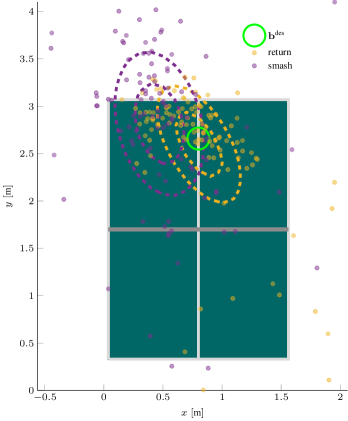
(a)

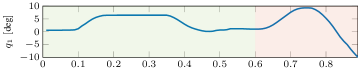
(b)

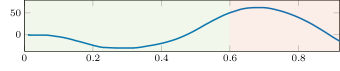
(c)

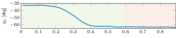
(d)

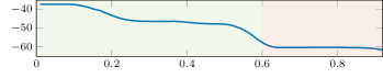
(e)

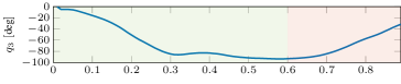
(f)

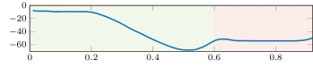
(g)

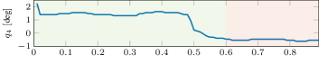
(h)

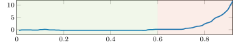
(i)

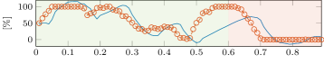
(j)

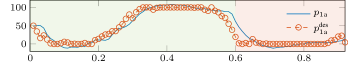
(k)

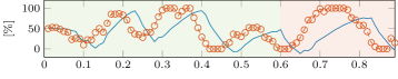
(l)

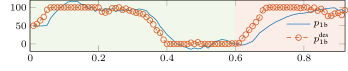
(m)

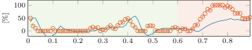
(n)

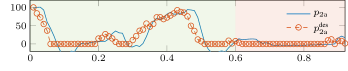
(o)

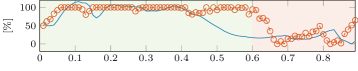
(p)

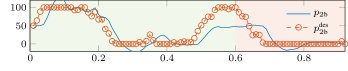
(q)

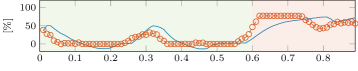
(r)

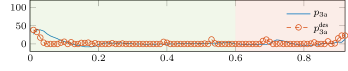
(s)

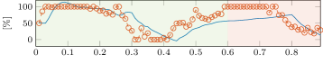
(t)

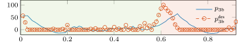
(u)

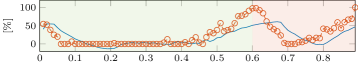
(v)

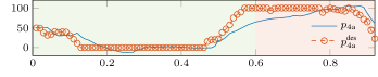
(w)

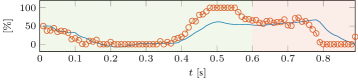
(x)

Figure 8: Joint angle and action trajectories of a single return (left) and smash (right) motion from Section III-A and Section III-B. The pressures are normalized between $[0\%\ldots 100\%]$ to indicate that pressure ranges which map to $[$0\text{\,}\mathrm{bar}$\ldots$3\text{\,}\mathrm{bar}$]$. The impact with the ball happens at $t=\sim$0.9\text{\,}\mathrm{s}$$ for the return and the smash. Green and red background color indicate the prepare and hit phase from Figure 6.

References

- [1] D. Silver, J. Schrittwieser, K. Simonyan, I. Antonoglou, A. Huang, A. Guez, T. Hubert, L. Baker, M. Lai, A. Bolton, Y. Chen, T. Lillicrap, F. Hui, L. Sifre, G. van den Driessche, T. Graepel, and D. Hassabis, “Mastering the game of Go without human knowledge,” Nature, vol. 550, no. 7676, pp. 354–359, Oct. 2017. [Online]. Available: https://www.nature.com/articles/nature24270
- [2] N. Heess, D. TB, S. Sriram, J. Lemmon, J. Merel, G. Wayne, Y. Tassa, T. Erez, Z. Wang, S. M. A. Eslami, M. Riedmiller, and D. Silver, “Emergence of Locomotion Behaviours in Rich Environments,” arXiv:1707.02286 [cs], Jul. 2017, arXiv: 1707.02286. [Online]. Available: http://arxiv.org/abs/1707.02286
- [3] S. Gu, E. Holly, T. Lillicrap, and S. Levine, “Deep Reinforcement Learning for Robotic Manipulation with Asynchronous Off-Policy Updates,” arXiv:1610.00633 [cs], Oct. 2016, arXiv: 1610.00633. [Online]. Available: http://arxiv.org/abs/1610.00633
- [4] OpenAI, M. Andrychowicz, B. Baker, M. Chociej, R. Jozefowicz, B. McGrew, J. Pachocki, A. Petron, M. Plappert, G. Powell, A. Ray, J. Schneider, S. Sidor, J. Tobin, P. Welinder, L. Weng, and W. Zaremba, “Learning Dexterous In-Hand Manipulation,” arXiv:1808.00177 [cs, stat], Aug. 2018, arXiv: 1808.00177. [Online]. Available: http://arxiv.org/abs/1808.00177
- [5] D. Schwab, T. Springenberg, M. F. Martins, T. Lampe, M. Neunert, A. Abdolmaleki, T. Hertweck, R. Hafner, F. Nori, and M. Riedmiller, “Simultaneously Learning Vision and Feature-based Control Policies for Real-world Ball-in-a-Cup,” arXiv:1902.04706 [cs, stat], Feb. 2019, arXiv: 1902.04706. [Online]. Available: http://arxiv.org/abs/1902.04706
- [6] C. Bodnar, A. Li, K. Hausman, P. Pastor, and M. Kalakrishnan, “Quantile QT-Opt for Risk-Aware Vision-Based Robotic Grasping,” arXiv:1910.02787 [cs, stat], Oct. 2019, arXiv: 1910.02787. [Online]. Available: http://arxiv.org/abs/1910.02787
- [7] A. Majumdar, S. Singh, A. Mandlekar, and M. Pavone, “Risk-sensitive Inverse Reinforcement Learning via Coherent Risk Models,” in Robotics: Science and Systems, 2017.
- [8] G. Dulac-Arnold, D. Mankowitz, and T. Hester, “Challenges of Real-World Reinforcement Learning,” arXiv:1904.12901 [cs, stat], Apr. 2019, arXiv: 1904.12901. [Online]. Available: http://arxiv.org/abs/1904.12901
- [9] S. Gomez-Gonzalez, G. Neumann, B. Schölkopf, and J. Peters, “Adaptation and Robust Learning of Probabilistic Movement Primitives,” arXiv:1808.10648 [cs, stat], Aug. 2018, arXiv: 1808.10648. [Online]. Available: http://arxiv.org/abs/1808.10648
- [10] K. Muelling, J. Kober, and J. Peters, “Learning table tennis with a Mixture of Motor Primitives,” in 2010 10th IEEE-RAS International Conference on Humanoid Robots (Humanoids), Dec. 2010, pp. 411–416.
- [11] K. Mülling, J. Kober, O. Kroemer, and J. Peters, “Learning to select and generalize striking movements in robot table tennis,” The International Journal of Robotics Research, vol. 32, no. 3, pp. 263–279, Mar. 2013. [Online]. Available: http://ijr.sagepub.com/content/32/3/263
- [12] Y. Huang, D. Büchler, O. Koç, B. Schölkopf, and J. Peters, “Jointly learning trajectory generation and hitting point prediction in robot table tennis,” in 2016 IEEE-RAS 16th International Conference on Humanoid Robots (Humanoids), Nov. 2016, pp. 650–655.
- [13] O. Koç, G. Maeda, and J. Peters, “Online optimal trajectory generation for robot table tennis,” Robotics and Autonomous Systems, vol. 105, pp. 121–137, Jul. 2018. [Online]. Available: http://www.sciencedirect.com/science/article/pii/S0921889017306164
- [14] J. Kober, K. Mülling, O. Krömer, C. H. Lampert, B. Schölkopf, and J. Peters, “Movement templates for learning of hitting and batting,” in 2010 IEEE International Conference on Robotics and Automation, May 2010, pp. 853–858.
- [15] O. Koç, G. Maeda, and J. Peters, “Optimizing the Execution of Dynamic Robot Movements With Learning Control,” IEEE Transactions on Robotics, vol. 35, no. 4, pp. 909–924, Aug. 2019.
- [16] D. Büchler, H. Ott, and J. Peters, “A Lightweight Robotic Arm with Pneumatic Muscles for Robot Learning,” in International Conference on Robotics and Automation (ICRA), Stockholm, May 2016.
- [17] D. Büchler, R. Calandra, and J. Peters, “Learning to Control Highly Accelerated Ballistic Movements on Muscular Robots,” arXiv:1904.03665 [cs], Apr. 2019, arXiv: 1904.03665. [Online]. Available: http://arxiv.org/abs/1904.03665
- [18] B. Tondu, “Modelling of the McKibben artificial muscle: A review,” Journal of Intelligent Material Systems and Structures, vol. 23, no. 3, pp. 225–253, Feb. 2012. [Online]. Available: http://jim.sagepub.com/content/23/3/225
- [19] D. Büchler, R. Calandra, B. Schölkopf, and J. Peters, “Control of Musculoskeletal Systems using Learned Dynamics Models,” IEEE Robotics and Automation Letters, 2018.
- [20] S. Gomez-Gonzalez, Y. Nemmour, B. Schölkopf, and J. Peters, “Reliable Real Time Ball Tracking for Robot Table Tennis,” arXiv:1908.07332 [cs], Aug. 2019, arXiv: 1908.07332. [Online]. Available: http://arxiv.org/abs/1908.07332
- [21] T. Senoo, A. Namiki, and M. Ishikawa, “Ball control in high-speed batting motion using hybrid trajectory generator,” in Proceedings 2006 IEEE International Conference on Robotics and Automation, 2006. ICRA 2006., May 2006, pp. 1762–1767.
- [22] G. Neumann, C. Daniel, A. Paraschos, A. Kupcsik, and J. Peters, “Learning Modular Policies for Robotics,” Frontiers in Computational Neuroscience, vol. 8, p. 62, 2014. [Online]. Available: http://journal.frontiersin.org/Journal/10.3389/fncom.2014.00062/pdf
- [23] S. Kawakami, M. Ikumo, and T. Oya, “Omron table tennis robot forpheus,” Tech. Rep., 2016. [Online]. Available: https://www.omron.com/innovation/forpheus.html
- [24] Y. Huang, D. Xu, M. Tan, and H. Su, “Adding Active Learning to LWR for Ping-Pong Playing Robot,” IEEE Transactions on Control Systems Technology, vol. 21, no. 4, pp. 1489–1494, Jul. 2013, conference Name: IEEE Transactions on Control Systems Technology.
- [25] K. Narioka, T. Homma, and K. Hosoda, “Humanlike ankle-foot complex for a biped robot,” in 2012 12th IEEE-RAS International Conference on Humanoid Robots (Humanoids 2012), Nov. 2012, pp. 15–20.
- [26] K. Mülling, J. Kober, and J. Peters, “A biomimetic approach to robot table tennis,” Adaptive Behavior, vol. 19, no. 5, pp. 359–376, Oct. 2011. [Online]. Available: http://adb.sagepub.com/content/19/5/359
- [27] J. Schulman, F. Wolski, P. Dhariwal, A. Radford, and O. Klimov, “Proximal Policy Optimization Algorithms,” arXiv:1707.06347 [cs], Jul. 2017, arXiv: 1707.06347. [Online]. Available: http://arxiv.org/abs/1707.06347
- [28] P. Dhariwal, C. Hesse, O. Klimov, A. Nichol, M. Plappert, A. Radford, J. Schulman, S. Sidor, and Y. Wu, “Openai baselines,” GitHub, GitHub repository, 2017.
- [29] Ramanantsoa and Durey, “Towards a stroke Construction Model,” ITTF Education, Jan. 1994. [Online]. Available: https://www.ittfeducation.com/towards-stroke-construction-model/
- [30] K. Muelling, A. Boularias, B. Mohler, B. Schölkopf, and J. Peters, “Learning strategies in table tennis using inverse reinforcement learning.” Biological cybernetics, 2014. [Online]. Available: http://www.ias.tu-darmstadt.de/uploads/Site/EditPublication/Muelling_BICY_2014.pdf