Sketchy Empirical Natural Gradient Methods for Deep Learning

Abstract

In this paper, we develop an efficient sketchy empirical natural gradient method (SENG) for large-scale deep learning problems. The empirical Fisher information matrix is usually low-rank since the sampling is only practical on a small amount of data at each iteration. Although the corresponding natural gradient direction lies in a small subspace, both the computational cost and memory requirement are still not tractable due to the high dimensionality. We design randomized techniques for different neural network structures to resolve these challenges. For layers with a reasonable dimension, sketching can be performed on a regularized least squares subproblem. Otherwise, since the gradient is a vectorization of the product between two matrices, we apply sketching on the low-rank approximations of these matrices to compute the most expensive parts. A distributed version of SENG is also developed for extremely large-scale applications. Global convergence to stationary points is established under some mild assumptions and a fast linear convergence is analyzed under the neural tangent kernel (NTK) case. Extensive experiments on convolutional neural networks show the competitiveness of SENG compared with the state-of-the-art methods. On the task ResNet50 with ImageNet-1k, SENG achieves 75.9% Top-1 testing accuracy within 41 epochs. Experiments on the distributed large-batch training show that the scaling efficiency is quite reasonable.

1 Introduction

Deep learning makes a breakthrough and holds great promise in many applications, e.g., machine translation, self-driving and etc. Developing practical deep learning optimization methods is an urgent need from end users.

The goal of deep learning is to find a fair good decision variable $\theta\in\mathbb{R}^{n}$ so that the output of the network $f(x,\theta)\in\mathbb{R}^{m}$ matches the true target $y$. Specifically, for a given dataset $\{x_{i},y_{i}\}_{i=1}^{N}$, we consider the following empirical risk minimization problem:

$$\min_{\theta\in\mathbb{R}^{n}}\Psi(\theta)=\frac{1}{N}\sum_{i=1}^{N}\psi_{i}(\theta)=\frac{1}{N}\sum_{i=1}^{N}\psi(y_{i},x_{i},\theta),$$ (1)

where $\psi_{i}(\theta)=\psi(y_{i},x_{i},\theta)$ is the loss function and it is common to use the negative log probability loss $\psi(y_{i},x_{i},\theta)=-\log\left(p\left(y_{i}|f\left(x_{i},\theta\right)\right)\right)$, e.g., the mean squared error (MSE) or the CrossEntropy loss.

The basic and most popular optimization methods in deep learning are first-order type methods, such as SGD (Robbins & Monro, 1951), Adam (Kingma & Ba, 2014), and etc. They are easy to implement but suffer a slow convergence rate and generalization gap in distributed large-batch training (Keskar et al., 2017; Shallue et al., 2019). Second-order type methods enjoy better convergence properties and exhibit a good potential in distributed large-batch training (Osawa et al., 2020), but suffer a high computational cost at each iteration. They leverage the curvature information in different ways. The natural gradient method (Amari, 1997) corrects the gradient according to the local KL-divergence surface. An online approximation to the natural gradient direction is used in the TONGA method (Roux et al., 2008). The online Newton step algorithm (Hazan et al., 2007) uses the empirical fisher information matrix (EFIM) and the authors analyze the convergence properties in the online learning setting. The Fisher Information Matrix (FIM) is integrated naturally with a practical Levenberg-Marquardt framework (Ren & Goldfarb, 2019) and the direction can be economically computed by using the Sherman-Morrison-Woodbury (SMW) formula. The KFAC method (Martens & Grosse, 2015) based on independence assumptions approximates the FIM by decomposing the large matrix into a Kronecker product between two smaller matrices each layer. A recursive block-diagonal approximation to the Gauss-Newton matrix is studied in (Botev et al., 2017) and each block is Kronecker factored.

Theoretical understanding of the second-order type methods for deep learning problems focuses on the natural gradient descent (NGD) methods. The authors in (Bernacchia et al., 2018) consider the deep linear networks and show the fast convergence of NGD. The properties of NGD for both shallow and deep nonlinear networks in the NTK regime are shown in (Zhang et al., 2019; Cai et al., 2019; Karakida & Osawa, 2020).

In this paper, we develop a novel Sketchy Empirical Natural Gradient (SENG) method. The EFIM is usually low-rank and thus the direction lies in a small subspace. However, the cost is not tractable due to the high dimensionality. Our SENG method utilizes randomized techniques to reduce the computational complexity and memory requirement. By using the SMW formula, it is easy to know that the search direction is actually a linear combination of the subsampled gradients where the coefficients are determined by a regularized least squares (LS) subproblem. For layers with a reasonable dimension, we construct a much smaller subproblem by sketching on the subsampled gradients. Otherwise, since the gradient is a vectorization of the product between two matrices, we first take low-rank approximations to these matrices and then use randomized algorithms to approximate the expensive operations. We further extend SENG to the distributed setting and propose suitable strategies to reduce both the communication and computational cost for extremely large-scale applications. Global convergence is established under some mild assumptions and the linear convergence rate is proved for the NTK case. Numerical comparisons with the state-of-the-art methods demonstrate the competitiveness of our method on a few typical neural network architectures and datasets. On the task of training ResNet50 on ImageNet-1k, we show great improvement over the well-tuned SGD (with momentum) method. Experiments on large-batch training are investigated to show the good scaling efficiency and the great potential in practice.

2 The Empirical Fisher Information Matrix

The FIM of the loss in (1) is based on the distribution learned by the neural network (Martens & Grosse, 2015; Martens, 2020) and is defined by: $\frac{1}{N}\sum_{i=1}^{N}\mathbb{E}_{y\sim p(y|x_{i},\theta)}\nabla_{\theta}\psi(y,x_{i},\theta)\nabla_{\theta}\psi(y,x_{i},\theta)^{\top},$ where the distribution $p(y|x,\theta)$ coincides with that used in the loss function. The subsampled FIM is also considered in the KFAC method (Martens & Grosse, 2015) and is defined as

$$\frac{1}{N}\sum_{i=1}^{N}\frac{1}{m_{i}}\sum_{j=1}^{m_{i}}\nabla_{\theta}\psi(y_{i}^{j},x_{i},\theta)\nabla_{\theta}\psi(y_{i}^{j},x_{i},\theta)^{\top},$$

where $y_{i}^{j}\sim p(y|x_{i},\theta)$ and $m_{i}$ is the number of the samples for $x_{i}$. Computing the subsampled FIM needs more backward passes. Instead, we consider the EFIM and use its low-rank subsampled variant as our curvature matrix. Given a mini-batch $S\subset\{1,2,\dots,N\}$ with a sample size $\varrho=|S|$, the subsampled EFIM can be represented as follows:

$$M_{S}(\theta)=\frac{1}{\varrho}\sum_{i\in S}\nabla\psi_{i}(\theta)\nabla\psi_{i}(\theta)^{\top}.$$ (2)

The subsampled EFIM (2) is a summation of a few rank-one matrices and is low-rank if $n\gg\varrho$. In practice, when the over-parameterized neural networks ($n\gg N$) are used, the deterministic EFIM ($\rho=N$) is still low-rank. Another important motivation is that the EFIM is a part of the Hessian matrix in certain cases e.g., for the negative log probability loss, $\nabla^{2}\Psi(\theta)=\frac{1}{N}\sum_{i=1}^{N}\left(\nabla\psi_{i}(\theta)\nabla\psi_{i}(\theta)^{\top}-\frac{1}{p\left(y_{i}|f\left(x_{i},\theta\right)\right)}\frac{\partial^{2}p\left(y_{i}|f\left(x_{i},\theta\right)\right)}{\partial\theta^{2}}\right).$ Considering a neural network with $L$ layers, the gradient with respect to (w.r.t.) the layer $l$ for a single sample $\{x_{i},y_{i}\}$ can be obtained by the back-propagation process and written as a vectorization of matrix-matrix multiplication (Sun, 2019)

$$u_{i}^{l}(\theta)=\operatorname{vec}(\hat{G}^{l}_{i}(\theta)(\hat{A}^{l}_{i}(\theta))^{\top}),$$ (3)

where $\hat{G}_{i}^{l}(\theta)\in\mathbb{R}^{n^{l}_{G}\times\kappa^{l}}$, $\hat{A}_{i}^{l}(\theta)\in\mathbb{R}^{n_{A}^{l}\times\kappa^{l}}$, $n^{l}=n^{l}_{G}\cdot n^{l}_{A}$ and $n^{l}$ is the number of parameters in the $l$-th layer. Note that $\hat{G}^{l}_{i}(\theta)$ and $\hat{A}^{l}_{i}(\theta)$ are computed by the backward and forward process, respectively. Hence, the per-sample gradient is a concatenation of $L$ sub-vectors:

$$\nabla\psi_{i}(\theta):=u_{i}(\theta)$$

$$=[(u_{i}^{1}(\theta))^{\top},\dots,(u_{i}^{l}(\theta))^{\top},\dots,(u_{i}^{L}(\theta))^{\top}]^{\top}\in\mathbb{R}^{n}.$$

Hence, the subsampled EFIM matrix $M_{S}(\theta)$ and its block diagonal part can be written as:

$$M_{S}(\theta) =\frac{1}{\varrho}\sum_{i\in S}u_{i}(\theta)u_{i}(\theta)^{\top}=U_{S}(\theta)U_{S}(\theta)^{\top},$$ (4)

and

$$M^{l}_{S}(\theta) =\frac{1}{\varrho}\sum_{i\in S}u^{l}_{i}(\theta)u^{l}_{i}(\theta)^{\top}=U^{l}_{S}(\theta)U^{l}_{S}(\theta)^{\top},$$ (5)

where $U_{S}(\theta)=\frac{1}{\sqrt{\varrho}}[u_{1}(\theta),u_{2}(\theta),\ldots,u_{\varrho}(\theta)]\in\mathbb{R}^{n\times\varrho}$ and $U^{l}_{S}(\theta)=\frac{1}{\sqrt{\varrho}}[u_{1}^{l}(\theta),u_{2}^{l}(\theta),\dots,u_{\varrho}^{l}(\theta)]\in\mathbb{R}^{n^{l}\times\varrho}$.

Note that the subscript $S$ and $\theta$ will be dropped if no confusion can arise. For example, we denote $M_{S^{k}}^{l}(\theta_{k})$ by $M_{k}^{l}$ at the point $\theta_{k}$. Throughout this paper, the layer number is expressed by the superscripts.

3 The SENG Methods

We first describe a second-order framework for the problem (1). At the $k$-th iteration, a regularized quadratic minimization problem at the point $\theta_{k}$ is constructed as follows:

$$\min_{d}F_{k}(d)=\Psi_{k}+g_{k}^{\top}d+\frac{1}{2}d^{\top}(B_{k}+\lambda_{k}I)d,$$ (6)

where $\Psi_{k}=\Psi(\theta_{k})$, $g_{k}=g_{S_{k}}(\theta_{k})=\frac{1}{|S_{k}|}\sum_{i\in S_{k}}u_{i}(\theta_{k})$ is the mini-batch gradient, $B_{k}$ is an approximation to the Hessian matrix of $\Psi$ at $\theta_{k}$ and $\lambda_{k}$ is a regularization parameter to make $B_{k}+\lambda_{k}I$ positive definite. Note that the sample sets in the $B_{k}$ and $g_{k}$ can be different. To reduce the computational cost, $B_{k}$ is designed to be block diagonal according to the network structure:

$$B_{k}=\text{block-diag}\{M^{1}_{k},\dots M^{L}_{k}\}.$$

Hence, $B_{k}$ is positive semi-definite. By solving the subproblem (6), we obtain $d_{k}:=[(d_{k}^{1})^{\top},\dots,(d_{k}^{L})^{\top}]^{\top}$, where

$$d_{k}^{l}=-(M_{k}^{l}+\lambda_{k}I)^{-1}g_{k}^{l}.$$ (7)

Then we set $\theta_{k+1}=\theta_{k}+\alpha_{k}d_{k}$, where $\alpha_{k}$ is the step size. Since the formulations of the directions $d_{k}^{l}$ for all layers are identical, we next only focus on a single layer by dropping the explicit layer indices and the iteration number $k$ if no confusion can arise. For example, $n^{l}$ and $U_{k}^{l}$ are written as $n$ and $U$ for simplicity in certain cases.

3.1 Direction in a Low-rank Subspace

The main concern in (7) is the expensive computation of the inverse of $M$. However, considering the low-rank structure of $M$ in (5) and by the SMW formula, the direction actually is:

$$d=-ag+aUb,$$ (8)

where $a=\frac{1}{\lambda}$ is a scalar and

$$b=(\lambda I+U^{\top}U)^{-1}(U^{\top}g)\in\mathbb{R}^{\varrho}.$$ (9)

Thus, the direction $d$ is located in a low-rank subspace spanned by $g$ and the column space of $U$.

This computation involves three basic operations: $U^{\top}z$, $U^{\top}U$ and $Uc$ for certain vectors $z$ and $c$. The main cost is the computation of the coefficients $b$, whose complexity is $O(\varrho^{3}+\varrho^{2}n)$. Since the batch size $\varrho$ is not large in many cases, the bottleneck in (9) is computing the product $U^{\top}U$ rather than computing the inverse of a $\varrho\times\varrho$ matrix.

The number of parameters $n$ for each layer is usually very large, see Table 1. Therefore, both the computational cost and memory requirement of $U$ can not be ignored due to the high dimensionality. When $n$ is large and $n>(n_{G}+n_{A})\kappa$, e.g., for the cases IV, V, VI in Table 1, it is better to store $\hat{G_{i}}$ and $\hat{A}_{i}$ other than the gradient $u_{i}$. Otherwise, e.g., for the cases I, II, III in Table 1, we store $U$ explicitly and the computational cost can be reduced by sketching. We next present explicit and implicit methods for both cases by designing different sketching mechanisms in Sec 3.2 and Sec 3.3, respectively.

Table 1: Statistics on a few typical layers of ResNet50. Conv means the convolutional layer while Fc means the fully-connected layer.

Case	$n^{l}$	$n_{G}^{l}$	$n_{A}^{l}$	$\kappa^{l}$	Type
I	9, 408	64	147	12, 544	Conv
II	147, 456	128	1, 152	784	Conv
III	524, 288	1, 024	512	196	Conv
IV	1, 048, 576	2, 048	512	49	Conv
V	2, 359, 296	512	4, 608	49	Conv
VI	2, 049, 000	1, 000	2, 049	1	Fc

3.2 Sketching on a Regularized LS Subproblem

In this part, we use sketching on a regularized least squares subproblem to reduce the computational cost of $b$. This is based on the key observation that the vector $b$ in (8) is the solution of the following regularized LS problem:

$$\min_{b\in\mathbb{R}^{\varrho}}\|Ub-g\|^{2}+\lambda\|b\|_{2}^{2}.$$ (10)

We use the sketching method to reduce the scale of the subproblem by denoting $\Xi=\Omega U$, $\xi=\Omega g$, where $\Omega\in\mathbb{R}^{q\times n}$ is a sketching matrix ($q\ll n$). Then, the subproblem is modified as:

$$\min_{\hat{b}\in\mathbb{R}^{\varrho}}\|\Omega U\hat{b}-\Omega g\|^{2}+\lambda\|\hat{b}\|_{2}^{2}=\|\Xi\hat{b}-\xi\|^{2}+\lambda\|\hat{b}\|^{2}.$$ (11)

The solution of the problem (11) is

$$\hat{b}=\left(\lambda I+\Xi^{\top}\Xi\right)^{-1}\Xi^{\top}\xi.$$ (12)

Hence, the direction is changed to:

$$\hat{d} =-ag+aU\hat{b}.$$ (13)

Replacing (10) by (13), the complexity of calculating the coefficients is reduced from $O(\varrho^{2}n)$ to $O(\varrho^{2}q)$.

Construction of $\Omega$. We consider random row samplings where the rows of $\Omega_{i,:},\;i=1,2,\dots,q,$ are sampled from

$$\omega\leftarrow\frac{e_{i}^{\top}}{p_{i}},i=1,2,\dots,n,$$ (14)

with/without replacement, where $\{p_{j}\}$ are given sampling probabilities. Two common strategies are listed below:

• Uniform sampling: All $p_{i}$ are the same and $p_{i}=\frac{1}{n},\;\forall i=1,2,\dots,n$.

• Leverage score sampling: Each $p_{i}$ is proportional to the row norm squares $\|U_{i,:}\|_{2}^{2}$, where $U_{i,:}$ is the $i$-th row of $U$, that is, $p_{i}=\frac{\|U_{i,:}\|_{2}^{2}}{\sum_{i=1}^{n}\|U_{i,:}\|_{2}^{2}}$.

In fact, the kinds of the sketching methods do not have a strong influence on the performance. Moreover, sketching the matrix $U$ by row sampling is cheap.

3.3 Implicit Computation and Storage of $U$ to Reduce Complexity

Although the computational complexity is reduced by sketching, the memory consumption in (13) is still large in certain cases. In this part, we take advantage of the structure of the gradient to reduce the memory usage.

We first assume that each element of $U_{S}$ can be approximated as follows:

$$u_{i}=\operatorname{vec}\left(\hat{G_{i}}\hat{A}_{i}^{\top}\right)\approx\operatorname{vec}\left(G_{i}A_{i}^{\top}\right)=\sum_{j=1}^{r}{a}_{ij}\otimes{g}_{ij},$$ (15)

where ${G}_{i}=[{g}_{i1},\ldots,{g}_{ir}]\in\mathbb{R}^{n_{G}\times r}$, ${A}_{i}=[{a}_{i1},\ldots,{a}_{ir}]\in\mathbb{R}^{n_{A}\times r}$ and $r\leq\kappa$.

We next describe sketching methods to compute $U^{\top}z$, $U^{\top}U$ and $Uc$ for any vector $z,c$ by using $\{G_{i},A_{i}\}$. Denote

$$\widetilde{A} =[A_{1},A_{2},\dots,A_{\varrho}]\in\mathbb{R}^{n_{A}\times r\varrho},$$ (16)

$$\widetilde{G} =[G_{1},G_{2},\dots,G_{\varrho}]\in\mathbb{R}^{n_{G}\times r\varrho}.$$

When $n_{A}$ or $n_{G}$ is large, we sample the rows of $\widetilde{G}$ and $\widetilde{A}$ with two sketching matrices $\Omega_{G}\in\mathbb{R}^{\zeta_{G}\times n_{G}}$ and $\Omega_{A}\in\mathbb{R}^{\zeta_{A}\times n_{A}}$. Hence, we obtain

$$\Xi_{\widetilde{A}} =\Omega_{A}\widetilde{A}=[\Xi_{A_{1}},\dots,\Xi_{A_{\varrho}}],$$ (17)

$$\Xi_{\widetilde{G}} =\Omega_{G}\widetilde{G}=[\Xi_{G_{1}},\dots,\Xi_{G_{\varrho}}],$$

where $\Xi_{G_{i}}=\Omega_{G}G_{i}$ and $\Xi_{A_{i}}=\Omega_{A}A_{i}$. When $n_{A}$ and $n_{G}$ are already small enough, we simply let $\Xi_{\widetilde{A}}=\widetilde{A}$ and $\Xi_{\widetilde{G}}=\widetilde{G}$.

Computation of $U^{\top}z$. We sketch $\texttt{mat}(z)$ with the same sketching matrices and define $\Xi_{z}=\Omega_{G}\texttt{mat}(z)\Omega_{A}^{\top}$, where $\texttt{mat}(\cdot):\mathbb{R}^{n}\rightarrow\mathbb{R}^{n_{G}\times n_{A}}$. By the randomized techniques, the $i$-th element of $U^{\top}z$ can be approximated as:

$$u_{i}^{\top}z \approx\sum_{j=1}^{r}{g}_{ij}^{\top}\texttt{mat}(z){a}_{ij}$$ (18)

$$\approx\texttt{elesum}\left(\left(\Xi_{z}^{\top}\Xi_{G_{i}}\right)\odot(\Xi_{A_{i}})\right),$$ (19)

where $\odot$ is the Hadamard product and $\texttt{elesum}(X)=\sum_{ij}X_{ij}$.

Computation of $U^{\top}U$. Similarly, the $(i,j)$ element of $U^{\top}U$ is approximated as:

$$(u_{i})^{\top}u_{j} \approx\left(\sum_{k=1}^{r}a_{ik}\otimes g_{ik}\right)^{\top}\left(\sum_{k=1}^{r}a_{jk}\otimes g_{jk}\right)$$ (20)

$$\approx\texttt{elesum}\left((\Xi_{A_{i}}^{\top}\Xi_{A_{j}})\odot(\Xi_{G_{i}}^{\top}\Xi_{G_{j}})\right).$$ (21)

Computation of $Uc$. To compute $Uc$, we first have to compute the per-sample gradient $u_{i}$ for all $i\in S$, multiply them with corresponding $c_{i}$ and finally sum them together:

$$Uc=\sum_{i\in S}u_{i}c_{i}\approx\sum_{i\in S}\operatorname{vec}({G}_{i}{A}_{i}^{\top})c_{i}.$$ (22)

The process (22) is expensive since it requires the computation of $\varrho$ matrix-matrix products and vectorizations as well. When the dimension $n$ is large, the computational cost is not tractable. Alternatively, we assume $A_{i}$ and $G_{i}$ are independent and approximate $Uc$ by $\mathcal{C}_{U}(c)$, i.e., the product between the weighted averages of $G_{i}$ and $A_{i}$:

$$\mathcal{C}_{U}(c)=\operatorname{vec}\left(\sum_{i\in S}\sqrt{|c_{i}|}G_{i}\right)\left(\sum_{i\in S}\frac{c_{i}}{\sum_{i=1}^{\varrho}\sqrt{|c_{i}|}}A_{i}\right)^{\top}.$$ (23)

Therefore, an explicit calculation and storage of $u_{i}$ is avoided, and only one matrix-matrix multiplication is needed.

Let $\mathcal{A}_{\Omega_{A},\Omega_{G},U}(z)$ and $\mathcal{B}_{\Omega_{A},\Omega_{G},U}$ be the approximation of $U^{\top}z$ by (19) and $U^{\top}U$ by (21). Combining them with (23), the direction can be obtained as follows:

$$\hat{d}=-\frac{1}{\lambda}g+\mathcal{C}_{U}(\hat{b}),$$ (24)

where $\hat{b}=(\mathcal{B}_{\Omega_{A},\Omega_{G},U}+\lambda I)^{-1}\mathcal{A}_{\Omega_{A},\Omega_{G},U}(g)$. Note that (19) and (21) are equal to $((\Omega_{A}\otimes\Omega_{G})u_{i})^{\top}((\Omega_{A}\otimes\Omega_{G})z)$ and $((\Omega_{A}\otimes\Omega_{G})u_{i})^{\top}((\Omega_{A}\otimes\Omega_{G})u_{j})$, respectively. Therefore, the computation of $\hat{b}$ here can be seen as a special case of (12) by choosing $\Omega=(\Omega_{A}\otimes\Omega_{G}).$

1 INPUT: Curvature matrix update frequency $T$, threshold $\mathcal{T}$ and regularization $\lambda_{k}$.

for layer $l=0,1,...,L$ do

       if $n^{l}<\mathcal{T}$  then 

        if  $k$ mod T $=0$ then 

         construct $U_{k}^{l}$ based on the sample set $\tilde{S}_{k}$ ;

        else 

         set $U_{k}^{l}=U_{k-1}^{l}$ ;

        Construct the sketching matrix $\Omega^{l}_{k}$ by (14);

        Solve the sketched least squares problem(11);

        Set $\hat{d}_{k}^{l}$ by (13) ;

       else 

        if  $k$ mod T $=0$ then 

         update $\widetilde{A}_{k}^{l},\widetilde{G}_{k}^{l}$ by the set $\tilde{S}_{k}$ and (16);

        else 

         set $\widetilde{A}_{k}^{l}=\widetilde{A}_{k-1}^{l}$ and $\widetilde{G}_{k}^{l}=\widetilde{G}_{k-1}^{l}$;

        Construct $(\Omega_{G})^{l}_{k}$ and $(\Omega_{A})^{l}_{k}$ by (14);

        Compute $\hat{d}_{k}^{l}$ by (24) ;

      

7OUTPUT: $\hat{d}_{k}:=[(\hat{d}_{k}^{1})^{\top},\dots,(\hat{d}_{k}^{L})^{\top}]^{\top}$.

Algorithm 1 The Computation of the Direction

We summarize the computation of the direction $\hat{d}$ in Algorithm 1 and SENG in Algorithm 2, respectively.

1 INPUT: Initial parameter $\theta_{1}$, step size $\{\alpha_{k}\}$ and regularization $\{\lambda_{k}\}.$

for $k=1,...,T$ do

      2 Choose the samples $S_{k}$ and compute $g_{k}$;

      3 Compute the direction $\hat{d}_{k}$ by Algorithm 1;

      4 Set $\theta_{k+1}=\theta_{k}+\alpha_{k}\hat{d}_{k}$;

5OUTPUT: $\theta_{T+1}$.

Algorithm 2 The SENG Methods

3.4 Computational Cost and Memory Consumption

In this part, we summarize computational cost and memory consumption of our methods in Table 2. We can observe that the randomized methods reduce both the computational cost and memory usage.

The SENG method avoids the inversion of high dimensional matrices. The size of the matrices equals the batch size. In practice, this number is often set to be 32, 64 or 256, which means that the computational cost of the matrix inversion is not a bottleneck. Instead, the matrix-matrix multiplications are required each iteration, but the cost is alleviated by our proposed sketching strategies. Note that the matrix inversion is the main computational cost in KFAC method. For example, the sizes of matrices to be inverted are 4, 608 and 512 for the case V in Table 1. Since the cost of matrices multiplications is usually smaller than that of the matrix inversion, generally speaking, the SENG methods can show greater advantages in large neural networks where the matrix inversion takes up most of the computational time.

4 Distributed SENG

In this section, we extend our methods to the distributed setting. Assume that $\mathcal{M}$ parallel workers are available and the samples $S_{k}$ are allocated to the $\mathcal{M}$ workers evenly, that is, $S_{k}=[S_{k,1},S_{k,2},\dots,S_{k,\mathcal{M}}],$ where $S_{k,i}$ is the samples in the $i$-th worker. The corresponding mini-batch gradient and the collection of gradients are also computed and stored in different workers accordingly

$$g_{k}=\frac{1}{\mathcal{M}}\sum_{i=1}^{\mathcal{M}}g_{S_{k,i}},\ \qquad U_{k}=[U_{S_{k,1}},\dots,U_{S_{k,\mathcal{M}}}].$$

Then, the direction in (8) can be rewritten as follows

$$d_{k} =-a_{k}\frac{1}{\mathcal{M}}\sum_{i=1}^{\mathcal{M}}g_{S_{k,i}}+a_{k}\frac{1}{\mathcal{M}}\sum_{i=1}^{\mathcal{M}}U_{S_{k,i}}b_{k,i}.$$ (25)

where $a_{k}=\frac{1}{\lambda_{k}}$, $b_{k}=[b_{k,1}^{\top},\dots,b_{k,\mathcal{M}}^{\top}]^{\top},\;b_{k,i}\in\mathbb{R}^{|S_{k,i}|}$.

To compute $U_{k}^{\top}U_{k}$ in (9), we need compute $U_{S_{k,i}}^{\top}U_{S_{k,j}}$ for all $i,j=1,\dots,\mathcal{M}$. However, since $U_{S_{k,j}}$ is stored by different workers, extensive communication cost is required among them. In the next, we use the block approximation to overcome this difficulty.

4.1 Distributed SENG Algorithm

Block Diagonal Approximation to $U^{\top}U.$

A direct idea is to use a diagonal approximation of $U_{k}^{\top}U_{k}$ to calculate the components $b$ in (9). Specifically, $(\lambda_{k}I+U_{k}^{\top}U_{k})^{-1}$ is approximated by a block-diagonal matrix with $\mathcal{M}$ blocks and

$$b_{k}\approx\text{block-approx}\left\{(\lambda_{k}I+U_{k}^{\top}U_{k})^{-1}\right\}(U_{k}^{\top}g_{k}):=\hat{b}_{k}.$$ (26)

Since $\hat{b}_{k,i}$ only relates to $U_{k,i}$ and $g_{k}$, once $g_{k}$ is available, we can compute $\hat{b}_{k}$ and further calculate $U_{S_{k,i}}\hat{b}_{k,i}$ simultaneously. Therefore, the direction can be obtained by averaging (All-Reduce) them among all workers by (25). The extra communication traffic is one tensor with the same size as the gradient and this synchronization is done separately from that of the gradient.

Table 2: A summary of the computational and memory complexity.

	Computational Cost	Memory Consumption
Low-rank Computation (8)	$\varrho^{3}+\varrho^{2}n$	$\varrho n$
Original LS (10)	$\varrho^{2}n$	$\varrho n$
Sketchy LS (11)	$\varrho^{2}q$	$\varrho n$
$U^{\top}z$	$\varrho n$	$\varrho n$
$U^{\top}z$ (18)	$n_{A}n_{G}\varrho r$	$(n_{A}+n_{G})r\varrho$
Randomized $U^{\top}z$ (19)	$\zeta_{A}\zeta_{G}\varrho r$	$(\zeta_{A}+\zeta_{G})r\varrho$
$U^{\top}U$	$\varrho^{2}n$	$\varrho n$
$U^{\top}U$ (20)	$r^{2}\varrho^{2}(n_{A}+n_{G})$	$(n_{A}+n_{G})r\varrho$
Randomized $U^{\top}U$ (21)	$r^{2}\varrho^{2}(\zeta_{A}+\zeta_{G})$	$(\zeta_{A}+\zeta_{G})r\varrho$
$Uc$	$\varrho n$	$\varrho n$
$Uc$ (22)	$n_{A}n_{G}r\varrho$	$(n_{A}+n_{G})r\varrho$
$Uc$ (23)	$n_{A}n_{G}r$	$(n_{A}+n_{G})r\varrho$

We further consider a distributed variant which has the same communication cost and the extra tensor can be synchronized simultaneously with the gradient. The coefficient $b_{k}$ is approximated by using the gradient $g_{k-1}$ in the last step as:

$$b_{k}\approx\text{block-approx}\left\{(\lambda_{k}I+U_{k}^{\top}U_{k})^{-1}\right\}(U_{k}^{\top}g_{k-1}):=\tilde{b}_{k}.$$ (27)

The sketching method presented in Sec 3.2 can be used naturally in the above distributed algorithms by replacing $U_{S_{k,i}}$ by $\Omega_{k}U_{S_{k,i}}$ in (26) and (27). If we use the implicit computation and storage of $U_{k}$ in Sec 3.3, the diagonal approximation to $U_{k}^{\top}U_{k}$ can also be applied to (21).

Computation of $U^{\top}z$ can be the same way as that in Sec 3.2 or Sec 3.3.

Computation of $Uc$

For the layers that use the explicit mechanisms, the operation $Uc$ is the same as (25). Otherwise, we use a new mechanism to overcome the communication in the summation of the absolute values $c_{k}$ presented in (23). We first compute $(G^{c})_{i}=\sum_{j\in S_{k,i}}\sqrt{|c_{j}|}G_{j}$ and $(A^{c})_{i}=\sum_{j\in S_{k,i}}\frac{c_{j}}{\sum_{i=1}^{|S_{k,i}|}\sqrt{|c_{j}|}}A_{j}$ in different workers, then synchronize them and approximate $Uc$ as:

$$Uc\approx\operatorname{vec}\left(\sum_{i=1}^{\mathcal{M}}(G^{c})_{i}\right)\left(\sum_{i=1}^{\mathcal{M}}(A^{c})_{i}\right)^{\top}.$$ (28)

5 Convergence Analysis

The convergence analysis of SENG is established in this section. We first prove that for the general objective function $\Psi(\theta)$, the algorithm converges to the stationary point globally. Furthermore, it is shown that the SENG method can converge to the optimal solution linearly under some mind conditions in the fully-connected neural network.

5.1 Global Convergence

In this part, we show the global convergence when $g_{k}$ is the unbiased mini-batch gradient. We assume the directions for all layers are obtained by the sketched subproblem (11) in Sec 3.2. Since the update rules for all layers are identical, we only consider one layer and drop the layer indices. The main idea of our proof is to first estimate the error between $d_{k}$ (8) and $\hat{d}_{k}$ (12), and the descent of the function values, then balance them by choosing a suitable step size. We give some necessary assumptions below.

Assumption 1.

Let $\eta_{k},\epsilon_{k}\in(0,1)$. Let $v$ be any fixed vector and $N_{k}\in\mathbb{R}^{n\times\rho_{k}}$ be an orthogonal basis for the column span of $U_{k}$, where $\rho_{k}=\text{rank}(U_{k}).$ Let $\Omega_{k}\in\mathbb{R}^{q_{k}\times n}$ be a sketching matrix, where the sample size $q_{k}$ depends on $\eta_{k}$, $\epsilon_{k}$ and $\delta_{k}$. The following two assumptions hold for all $k$ with a probability $1-\delta_{k}$:

• $\|N_{k}^{\top}\Omega_{k}^{\top}\Omega_{k}N_{k}-I\|_{2}\leq\eta_{k},$

• $\|N_{k}^{\top}\Omega_{k}^{\top}\Omega_{k}v-N_{k}^{\top}v\|^{2}_{2}\leq\epsilon_{k}\|v\|_{2}^{2}.$

Assumptions A.1-A.2 are called subspace embedding property and matrix multiplication property, respectively. They are standard in related sketching methods (Wang et al., 2017a, 2016). When the sample size $q_{k}$ is large enough, Assumptions A.1 and A.2 will be satisfied. Throughout the paper, we assume the sketching matrices are independent from each other and from the stochastic gradients. The sequence $\{\theta_{k}\}$ do not affect the stochasticity of $\mathbf{\Omega}=\{\Omega_{k}\}_{k=1}^{\infty}$.

Assumption 2.

• $\Psi$ is continuously differentiable on $\mathbb{R}^{n}$ and is bounded from below. The gradient $\nabla\Psi$ is Lipschitz continuous on $\mathbb{R}^{n}$ with modulus $L_{\Psi}\geq 1$.

• There exists positive constants $h_{1},h_{2}$ such that the matrix holds: $h_{1}I\preceq(B_{k}+\lambda_{k}I)\preceq h_{2}I$ for all k.

• $B_{k}$ and $g_{k}$ are independent for any iteration $k$. In addition, it holds almost surely that the stochastic gradient is unbiased, i.e., $\mathbb{E}[g_{k}|{\theta_{k-1},\dots,\theta_{0}},\mathbf{\Omega}]=\nabla\Psi(\theta_{k})$ and the variance of the stochastic gradient is bounded:

  $$\mathbb{E}[\|g_{k}-\nabla\Psi(\theta_{k})\|^{2}|{\theta_{k-1},\dots,\theta_{0}},\mathbf{\Omega}]\leq\sigma_{k}^{2}.$$

Assumptions B.1-B.3 are common in stochastic quasi-Newton type methods (Byrd et al., 2016; Wang et al., 2017b; Yang et al., 2019). We next summarize our analysis.

Theorem 3.

Suppose that Assumptions A.1-A.2 and B.1-B.3 are satisfied and $\frac{\sqrt{\epsilon_{k}}+\eta_{k}}{1-\eta_{k}}$ is small enough. If the step size $\{\alpha_{k}\}$ further satisfies $\alpha_{k}\leq\min\left\{\frac{1}{2L_{\Psi}},\frac{h_{1}^{2}}{2L_{\Psi}h_{2}}\right\}$, $\sum\alpha_{k}=\infty$ and $\sum\alpha_{k}\sigma_{k}^{2}<\infty,$ it holds

$$\lim_{k\rightarrow\infty}\nabla\Psi(\theta_{k})=0$$

with probability $\Pi_{k=0}^{\infty}(1-\delta_{k})$.

The proof of Theorem 3 is shown in the Appendix.

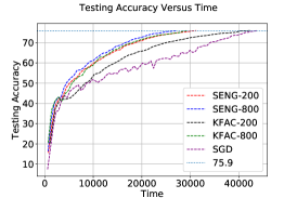
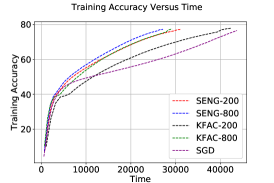
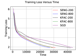
Figure 1: Numerical performance on ResNet50 on ImageNet-1k.

5.2 Linear Convergence in Wide Neural Networks

In this part, we analyze SENG for over-parameterized neural networks in the NTK regime. Consider a fully-connected network with a single output :

$$f(x,\theta)=\frac{1}{\sqrt{\hat{m}}}\sum_{i=1}^{\hat{m}}a^{i}\phi((w^{i})^{\top}x)=\frac{1}{\sqrt{\hat{m}}}a^{\top}\phi(Wx),$$

where $x\in\mathbb{R}^{m_{0}}$ is the input, $\phi$ is the Relu activation function and $a=[a^{1},\dots,a^{\hat{m}}]^{\top}\in\mathbb{R}^{\hat{m}}.$ $\theta=\operatorname{vec}{(W)}\in\mathbb{R}^{n}$ is the set of the learned parameters, where $W=[w^{1},\dots w^{\hat{m}}]$. For a given dataset $\{x_{i},y_{i}\}_{i=1}^{N}$, we consider the case where the loss is set to be MSE:

$$\Psi(\theta)=\frac{1}{2}\|f(\theta)-y\|_{2}^{2},$$ (29)

where $f(\theta)=[f(x_{1},\theta)^{\top},\dots,f(x_{N},\theta)^{\top}]^{\top}\in\mathbb{R}^{N}$ and $y=[y_{1}^{\top},\dots,y_{N}^{\top}]^{\top}\in\mathbb{R}^{N}.$ Denote $J(\theta)$ by the collections of Jacobian matrices $\frac{\partial f(\theta)}{\partial\theta}^{\top}\in\mathbb{R}^{n\times N}.$ Hence, the gradient can be written as $\nabla\Psi(\theta_{k})=J_{k}^{\top}(f^{k}-y),$ where $J_{k}=J(\theta_{k})$ and $f^{k}=f(\theta_{k}).$

Consider the SENG using (12) applied to $U_{k}=J_{k}^{\top}$ with $\alpha_{k}\equiv\alpha$. We next briefly explain a key step of our proof by deriving an equivalent format of the direction. The update rule is $\theta_{k+1}=\theta_{k}-\alpha d_{k},$ where $d_{k}=\frac{1}{\lambda_{k}}J_{k}^{\top}\left(I-(\lambda_{k}I+\widetilde{M}_{k})^{-1}\widetilde{M}_{k}\right)(f^{k}-y)$ and $\widetilde{M}_{k}=J_{k}\Omega_{k}^{\top}\Omega_{k}J_{k}^{\top}.$ Assume $\widetilde{M}_{k}$ is invertible and its eigenvalue decomposition is $Q_{k}\widetilde{\Sigma}_{k}Q_{k}$ where $Q_{k}$ is orthogonal and $\widetilde{\Sigma}_{k}$ is diagonal. Then, we obtain:

$$d_{k}= \frac{1}{\lambda_{k}}J_{k}^{\top}\left(Q_{k}\left(I-(\lambda_{k}I+\widetilde{\Sigma}_{k})^{-1}\widetilde{\Sigma}_{k}\right)Q_{k}^{\top}\right)(f^{k}-y)$$ (30)

$$= J_{k}^{\top}\left(Q_{k}(\lambda_{k}I+\widetilde{\Sigma}_{k})^{-1}Q_{k}^{\top}\right)(f^{k}-y),$$

where the second equality uses the fact that $\widetilde{\Sigma}_{k}$ is a diagonal matrix. The difference of SENG from NGD can be seen clearer by letting $\lambda_{k}\rightarrow 0$. Since $\widetilde{M}_{k}$ is positive definite due to over-parameterization, each diagonal entry of $\widetilde{\Sigma}_{k}$ is positive and we have:

$$d_{k}=J_{k}^{\top}\left(Q_{k}\widetilde{\Sigma}_{k}^{-1}Q_{k}^{\top}\right)(f^{k}-y)=J_{k}^{\top}\widetilde{M}_{k}^{-1}(f^{k}-y).$$

Note that the direction of NGD is $J_{k}^{\top}(J_{k}J_{k}^{\top})^{-1}(f^{k}-y)$, see (Zhang et al., 2019). Hence, the main difference is the occurrence of $\Omega_{k}^{\top}\Omega_{k}$ in $\widetilde{M}_{k}$.

Our convergence is established in the next theorem.

Theorem 4.

Assume that (1) the initialization $w_{0}^{i}\sim\mathcal{N}(0,\nu^{2}I)$, $a_{0}^{i}\sim\text{unif}\left(\{-1,+1\}\right)$ for $i=1,\dots,\hat{m}$; (2) the sketching matrices $\{\Omega_{k}\}$ are independent from the initialization; (3) each $\|x_{i}\|_{2}=1$, $|y_{i}|=\mathcal{O}(1)$ and $x_{i}\neq x_{i^{\prime}},\ \forall i\neq i^{\prime}$. Then, under the Assumptions A.1-A.2, if $\eta_{k}$, $\epsilon_{k}$ are small enough and $\hat{m}=\Omega\left(\frac{n^{4}}{\nu^{2}\lambda_{0}^{4}\delta^{3}}\right)$, it holds with a constant $\zeta\in(0,1)$,

$$\|f^{k}-y\|_{2}^{2}\leq\zeta^{k}\|f^{0}-y\|_{2}^{2}$$

with probability $(1-\delta)\Pi_{k=0}^{\infty}(1-\delta_{k})$ over the random initialization and the sketching.

The proof of Theorem 4 is shown in the Appendix. Here, $\lambda_{0}$ is the smallest eigenvalue of limiting Gram matrix. $\delta_{0}$ and $\delta_{k}$ are related to the weight initialization and sketching, respectively. The proof follows from (Zhang et al., 2019) by bounding two errors. One error is the difference between the natural gradient flow and the NGD sequence while the other is the difference between the sequence of NGD and that of the SENG. Theoretical understanding of SENG can be extended to the multi-layer fully-connected networks case similar to that in (Karakida & Osawa, 2020).

6 Numerical Experiments

In this part, we report the numerical results of SENG and make comparisons with the state-of-the-art methods. The performance is shown on the classical neural networks “ResNet18” and “VGG16_bn” with three commonly used datasets CIFAR10, CIFAR100 and SVHN. Furthermore, we consider the ResNet50 on ImageNet-1k classification problem and show the advantages over the SGD (with momentum) and KFAC. Our codes are implemented in PyTorch. We run ResNet18 and VGG16_bn experiments on one Tesla V100 GPU and ResNet50 on multiple Tesla V100 GPUs.

Table 3: Comparison of SENG on different batch sizes. We terminate the training when the top-1 testing accuracy achieves 75.9%. BS means batch size. TT means total time. TpE means time per epoch. Scaling efficiency (SE) for each line is $\frac{512}{BS(\cdot)}\times\frac{TT(512)}{TT(\cdot)}$ or $\frac{512}{BS(\cdot)}\times\frac{TpE(512)}{TpE(\cdot)}$.

BS	#GPUs	# Epochs	Total Time (TT)	SE (TT)	Time Per Epoch (TpE)	SE (TpE)
512	4	41	371.5 min	1	542.22 s	1
1024	8	41	202.4 min	0.92	296.12 s	0.92
2048	16	41	103.2 min	0.90	151.07 s	0.90
4096	32	41	49.7 min	0.93	72.66 s	0.93

6.1 ResNet18 & VGG16_bn

We demonstrate the comparison results of six tasks in this part. The compared methods are well-tuned by a grid search and the details can be found in the Appendix. We terminate the algorithms once their top-1 testing accuracy attains the given baseline. The related statistics are averages of three independent runs and shown in Table 4. We further show the the changes of testing accuracy and other statistics versus training time in the Appendix.

Table 4: Comparison with SGD, ADAM and KFAC on six tasks over three independent runs. “N” means the methods can not attain the given accuracy and the attained best testing accuracy is reported next to it. The time are in seconds.

	VGG16_bn
	SENG	SGD	ADAM	KFAC
CIFAR10 TimeTo92%	943.12	1034.82	N/89.4%	6009.86
Time/Epoch	17.49	14.58	16.13	113.37
CIFAR100 TimeTo70%	1088.16	1168.49	N/63.0%	5652.81
Time/Epoch	18.14	15.16	16.50	113.13
SVHN TimeTo95%	515.06	N/75.5%	N/94.97%	7321.62
Time/Epoch	24.43	20.30	22.56	162.57
	ResNet18
	SENG	SGD	ADAM	KFAC
CIFAR10 TimeTo94%	940.72	1083.60	N/91.3%	1040.24
Time/Epoch	16.48	15.04	15.39	19.67
CIFAR100 TimeTo76%	952.26	N/75.0%	N/68.4%	1001.44
Time/Epoch	16.70	14.99	15.14	19.27
SVHN TimeTo96%	685.29	1091.78	N/94.7%	1103.17
Time/Epoch	22.90	19.88	20.21	25.65

The performance of SENG is the best in all six tasks. Compared with first-order type methods, our SENG method takes fewer steps without too much overhead. The advantage of SENG in terms of the computational time over KFAC is also remarkable. For example, in CIFAR10 dataset with VGG16_bn, the time per epoch of SENG is 18 seconds while that of KFAC is 113.37 seconds. There exists large fully linear layers in the end of VGG16_bn, so that the cost of matrix inversions in the KFAC method dominates. By constrast, since the size of every matrix to be inverted in SENG is equal to the batch size, its computational time can be controlled.

Table 5: Detailed Statistics on ResNet50 on ImageNet-1k when the top-1 testing accuracy achieves 75.9%. The numbers that follows SENG and KFAC are the number of matrix update frequency.

	# Epochs	Total Time	Time Per Epoch
SENG-800	41	27, 190 s	663.17 s
SGD	76	43, 707 s	575.09 s
SENG-200	41	31, 224 s	761.56 s
KFAC-800	42	29, 204 s	712.29 s
KFAC-200	42	42, 307 s	1007.31 s

6.2 ResNet50 on ImageNet-1k

The training of ResNet50 on ImageNet-1k dataset is one of the base experiments in MLPerf (Mattson et al., 2019). We compare SENG with KFAC and SGD, and terminate the training process of all the three methods once the Top-1 testing accuracy equals or exceeds 75.9% as in the MLPerf requirement. The comparison with ADAM is not reported because it does not perform well in our numerical results.

We report the testing accuracy, training accuracy and training loss versus training time in Figure 1. The batch size is chosen to be $256$ for all the three methods and does not change during the training process. As shown in Figure 1, SENG performs best in the total training time and only takes 41 epochs to get 75.9% Top-1 testing accuracy. Detailed statistics can be found in Table 5. We can see the time per epoch of SENG is close to that of SGD while the number of epoch is much smaller. SENG is faster than KFAC using the same number of matrix update frequency because SENG does not require expensive matrix inversions. Note that the SGD reported here uses the cosine learning rate and its Top-1 testing accuracy can exceed 75.9% within 76 epochs, which is a well-tuned version. Detailed tuning strategies for SENG and KFAC can be found in the Appendix.

6.3 Scaling Efficiency

It has been widely known that large batch training will lead to performance degradation. In this part, we investigate the scalability of our proposed SENG. We start by running the codes with 4, 8 and 16 GPUs on one node, and then run the distributed version on 32 GPUs across 2 nodes. The results are shown in Table 3. We can see that the GPU scaling efficiency is over 90% in terms of both total time and time per epoch. The results show the great potential of SENG in the distributed large-batch training in practice.

It is noticed that SENG with the batch size 4, 096 can attain top-1 testing accuracy 75.9% within 41 epochs and takes 49.7 minutes. The number of epoch is the same on all batch sizes, which illustrates the effectiveness of SENG with large batch. Compared with the results reported in (Osawa et al., 2020) where SP-NGD with a batch size 4, 096 but on 128 Tesla V100 GPUs takes 32.5 minutes to top-1 testing accuracy 74.8%, our results are also reasonable. With more computational resources, it is expected that SENG can attain the given testing accuracy within less training time. The detailed hyper-parameters are reported in the Appendix.

7 Conclusion

In this paper, we develop efficient sketching techniques for the empirical natural gradient method for deep learning problems. Since the EFIM is usually low-rank, the corresponding direction is actually a linear combination of the subsampled gradients based on the SMW formula. For layers whose number of parameters is not huge, we construct a much smaller least squares problem by sketching on the subsampled gradients. Otherwise, the quantities in the SMW formula is computed by using the matrix-matrix representation of the gradients. We first approximate them by low-rank matrices, then use sketching methods to compute the expensive parts. Global convergence is guaranteed under some standard assumptions and a fast linear convergence is analyzed in the NTK regime. Our numerical results show that the empirical natural gradient method with randomized techniques can be quite competitive with the state-of-the-art methods such as SGD and KFAC. Experiments on the distributed large-batch training illustrate that the scaling efficiency of SENG is quite promising.

Acknowledgments M. Yang, D. Xu and Z. Wen are supported in part by Key-Area Research and Development Program of Guangdong Province (No.2019B121204008), the NSFC grants 11831002 and Beijing Academy of Artificial Intelligence.

Appendix A Implementation Details

The statistics of the datasets used in Section 6 are listed in Table 6.

Dataset	# Training Set	# Testing Set
CIFAR10	50,000	10,000
CIFAR100	50,000	10,000
SVHN	73,257	26,032
ImageNet-1k	1,281,167	50,000

Table 6: The Datasets Information.

We use the official implementation of VGG16_bn, ResNet18 and ResNet50 (also known as ResNet50 v1.5) in PyTorch. The detailed network structures can be found in the websites: https://pytorch.org/docs/stable/_modules/torchvision/models/resnet.html and https://pytorch.org/docs/stable/_modules/torchvision/models/vgg.html.

We next describe the tuning schemes of hyper-parameters. The learning rate is very important for performance and we mainly consider the following two schemes.

• cosine: Given the max_epoch and the initial learning rate $\alpha_{0}$, the learning rate $\alpha_{k}$ at the $k$-th epoch is changed as:

  $$\alpha_{k}=0.001+0.5*(\alpha_{0}-0.001)*(1+\text{cos(epoch\_k / max\_epoch}*\pi)).$$

• exp: Given the max_epoch, decay rate $\mathcal{\widetilde{D}}$ and the initial learning rate $\alpha_{0}$, the learning rate $\alpha_{k}$ at the $k$-th epoch is changed as:

  $$\alpha_{k}=\alpha_{0}*(1-\text{epoch\_k/max\_epoch)}^{\mathcal{\widetilde{D}}}.$$

• For ResNet18 and VGG16 on the three datasets, i.e., CIFAR10, CIFAR100 and SVHN:

  • Adam

    • The initial learning rate is chosen from {1e-4, 2e-4, 5e-4, 1e-3, 2e-3, 5e-3,1e-2, 2e-2, 5e-2, 1e-1}.

    • The parameters $\beta_{1}$ and $\beta_{2}$ are selected in {0.9,0.99} and $\{0.99,0.999\}$, respectively.

    • The weight decay is chosen from {5e-4, 2e-4,1e-4}.

    • The perturbation value $\epsilon$ is 1e-8.

  • SGD (with momentum): we use the best results from the cosine and exp schemes.

    • For the cosine scheme, the hyper-parameters is tuning as follows:

      • The initial learning rate is from {1e-3, 5e-3, 1e-2, 5e-2, 1e-1}.

      • The max_epoch is tuned from {85, 90}.

      • The weight decay is chosen from {5e-4, 2e-4,1e-4}.

      • The momentum is set to be 0.9.

    • For the exp scheme, the hyper-parameters is tuning as follows:

      • The initial learning rate in from {1e-3, 5e-3, 1e-2, 5e-2, 1e-1}.

      • The max_epoch is tuned from {70, 75, 80}.

      • The decay rate is tuned from {4, 5, 6}.

      • The weight decay is tuned from {5e-4, 2e-4,1e-4}.

      • The momentum is set to be 0.9.

  • KFAC and SENG use the same grid search strategies as SGD. In addition, the damping parameter for both methods is chosen from {1.5, 2.0, 2.5} for VGG16 and from { 0.8, 1.0,1.2} for ResNet18. KFAC updates the covariance matrix to be inverted every 200 iterations. Similarly, SENG updates the matrix $U$ at the same frequency. For convenience of notations, we call them the matrix update frequency for both methods. They are critical for the performance since the related operations are expensive.

• For ResNet50 on ImageNet-1k, we use the linear warmup strategy (Goyal et al., 2017) in the first 5 epochs for SGD, KFAC and SENG, then use the cosine or exp learning rate strategy.

  • SGD refers to a well-tuned cosine learning rate strategy in the website and the result reported here achieves top-1 testing accuracy 75.9% within 76 epochs. This is better than the result in terms of epoch in (Goyal et al., 2017) where they use the diminishing learning rate strategy and need nearly 90 epochs.

  • KFAC uses the exp strategy after the first 5 epochs. The initial learning rate is from {0.05, 0.1, 0.15} and the damping is from {0.05, 0.1, 0.15} and we report the best results among them.

  • SENG uses the exp strategy after the first 5 epochs. The initial learning rate is 0.145 and the damping is 0.17.

  • Note that both SENG and KFAC are not sensitive to damping and initial learning rate. The weight decay for SENG and KFAC are chosen the best from {5e-4, 3e-4, 2e-4, 1e-4}. We also consider the cosine strategy for KFAC and SENG, but it does not work well.

• For large-batch training, the detailed hyper-parameters for each batch-size are listed in Table 7.

  Batch Size	$\alpha_{\text{warmup}}$	$\alpha_{0}$	decay rate	max_epoch	damping $\lambda$
  512	0.01	0.3	6	60	0.17$\cdot(0.9)^{epoch/10}$
  1, 024	0.01	0.6	6	60	0.17$\cdot(0.9)^{epoch/10}$
  2, 048	0.2	1.2	6	60	0.3$\cdot(0.7)^{epoch/10}$
  4, 096	0.2	2.2	5	55	0.3$\cdot(0.7)^{epoch/10}$

  Table 7: Detailed hyper-parameters for different batch sizes.

Appendix B Further results in section 6

We give the other statistics on the six tasks in Figure 2. The comparison results with KFAC and SGD in section 6.2 with respect to other criteria are listed in Figure 3. The performance difference of SENG and KFAC in term of epoch is not significant since the matrix update frequency does not have a strong effect on the performance and the the changes of learning rate of both methods are very similar. The variants of SENG with different matrix update frequency are shown in Figure 4. The detailed results of SENG are reported in Table 8.

Table 8: Statistics of different matrix update frequency variants of SENG on ResNet50/ImageNet-1k when the top-1 Testing Accuracy achieves 75.9%.

Frequency (SENG)	100	200	500	800
# Epoch	40	41	42	41
Total Time	38, 586 s	31, 224 s	29, 332 s	27, 190 s
Time Per Epoch	964.65 s	761.56 s	698.38 s	663.17 s

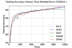
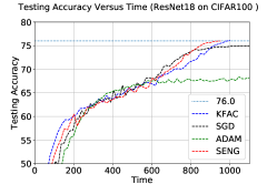
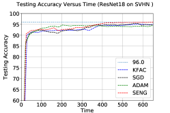
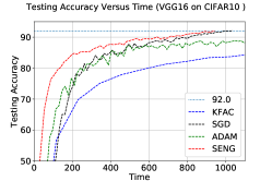
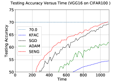
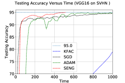
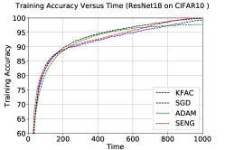
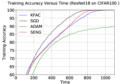
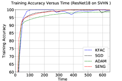
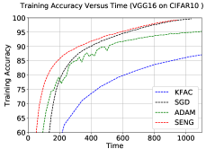
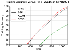
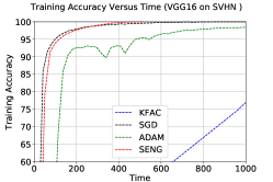
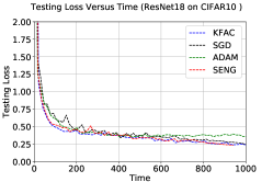
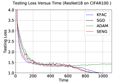
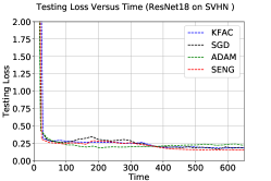
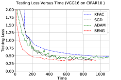
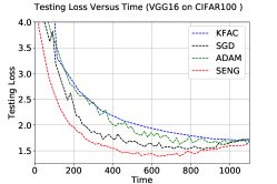
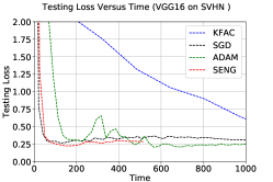
Figure 2: Numerical Comparison on six tasks in section 6.1.

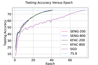
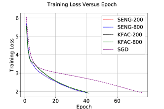
Figure 3: Numerical Comparison on ResNet50 on ImageNet-1k.

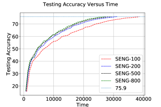
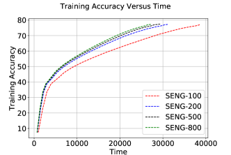
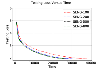
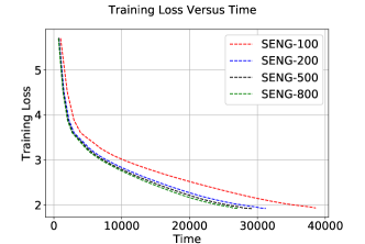
Figure 4: Numerical performance on ResNet50 on ImageNet-1k. The number behind SENG is the number of matrix update frequency.

Appendix C Proof of Theorem 3

We next estimate the error between $b_{k}$ in (9) and $\hat{b}_{k}$ in (12) and then establish the global convergence.

Lemma 5.

Suppose that Assumptions A.1, A.2 and B.2 are satisfied with $\eta_{k}$ and $\epsilon_{k}$. It holds

$$\|b_{k}-\hat{b}_{k}\|_{2}\leq\frac{\sqrt{\epsilon_{k}h_{1}}+\eta_{k}\sqrt{h_{1}}}{1-\eta_{k}}\|g_{k}\|_{2}$$ (31)

with probability at least $1-\delta_{k}$.

Proof.

The SVD decomposition of $U_{k}$ is: $U_{k}=N_{k}\Sigma_{k}V_{k},$ where $N_{k}\in\mathbb{R}^{n\times\rho_{k}},\Sigma_{k}\in\mathbb{R}^{\rho_{k}\times\rho_{k}},V_{k}\in\mathbb{R}^{\rho_{k}\times\varrho}$ and $\rho_{k}$ is the rank of $U_{k}$. Let $g_{k}^{\perp}=g_{k}-U_{k}U_{k}^{\dagger}g_{k}=g_{k}-N_{k}N_{k}^{\top}g_{k}$, where $U_{k}^{\dagger}$ is the pseudoinverse of $U_{k}$. By the definition in (9) and (12),

$$b_{k}=(\lambda_{k}I+U_{k}^{\top}U_{k})^{-1}(U_{k}^{\top}g_{k})\;\text{and}\;\hat{b}_{k}=(\lambda_{k}I+U_{k}^{\top}\Omega_{k}^{\top}\Omega_{k}U_{k})^{-1}(U_{k}^{\top}\Omega_{k}^{\top}\Omega_{k}g_{k}),$$

we have:

$$(\lambda_{k}I+U_{k}^{\top}\Omega_{k}^{\top}\Omega_{k}U_{k})(\hat{b}_{k}-b_{k})$$ (32)

$$= U_{k}^{\top}\Omega_{k}^{\top}\Omega_{k}g_{k}^{\perp}+U_{k}^{\top}\Omega_{k}^{\top}\Omega_{k}U_{k}U_{k}^{\dagger}g_{k}-(\lambda_{k}I+U_{k}^{\top}\Omega_{k}^{\top}\Omega_{k}U_{k})(\lambda_{k}I+U_{k}^{\top}U_{k})^{-1}U_{k}^{\top}g_{k}$$

$$= U_{k}^{\top}\Omega_{k}^{\top}\Omega_{k}g_{k}^{\perp}-\lambda_{k}U_{k}^{\dagger}g_{k}+(\lambda_{k}I+U_{k}^{\top}\Omega_{k}^{\top}\Omega_{k}U_{k})(\lambda_{k}I+U_{k}^{\top}U_{k})^{-1}[(\lambda_{k}I+U_{k}^{\top}U_{k})U_{k}^{\dagger}g_{k}-U_{k}^{\top}g_{k}]$$

$$= U_{k}^{\top}\Omega_{k}^{\top}\Omega_{k}g_{k}^{\perp}+\lambda_{k}(U_{k}^{\top}\Omega_{k}^{\top}\Omega_{k}U_{k}-U_{k}^{\top}U_{k})(\lambda_{k}I+U_{k}^{\top}U_{k})^{-1}U_{k}^{\dagger}g_{k}.$$

The last equality follows from the fact that $U_{k}^{\top}U_{k}U_{k}^{\dagger}g_{k}=U_{k}^{\top}g_{k}$. By Assumption B.2, we know $U_{k}^{\top}U_{k}+\lambda_{k}I$ is positive definite. We define:

$$(U_{k}^{\top}U_{k}+\lambda_{k}I)^{-1/2}(\lambda_{k}I+U_{k}^{\top}\Omega_{k}^{\top}\Omega_{k}U_{k})(\hat{b}_{k}-b_{k}):=\Pi_{k}+\Delta_{k},$$ (33)

where

$$\Pi_{k}= (U_{k}^{\top}U_{k}+\lambda_{k}I)^{-1/2}U_{k}^{\top}\Omega_{k}^{\top}\Omega_{k}g_{k}^{\perp}=V_{k}^{\top}(\Sigma_{k}^{2}+\lambda_{k}I)^{-1/2}\Sigma_{k}N_{k}^{\top}\Omega_{k}^{\top}\Omega_{k}g_{k}^{\perp}$$

$$\Delta_{k}= \lambda_{k}(U_{k}^{\top}U_{k}+\lambda_{k}I)^{-1/2}(U_{k}^{\top}\Omega_{k}^{\top}\Omega_{k}U_{k}-U_{k}^{\top}U_{k})(\lambda_{k}I+U_{k}^{\top}U_{k})^{-1}U_{k}^{\dagger}g_{k}$$

$$= \lambda_{k}V_{k}^{\top}\Sigma_{k}(\Sigma_{k}^{2}+\lambda_{k}I)^{-1/2}(N_{k}^{\top}\Omega_{k}^{\top}\Omega_{k}N_{k}-I)(\Sigma_{k}^{2}+\lambda_{k}I)^{-1}N_{k}^{\top}g_{k}.$$

By Assumption A.1, it holds with probability $1-\delta_{k}$:

$$(1-\eta_{k})I\preceq N_{k}^{\top}\Omega_{k}^{\top}\Omega_{k}N_{k}\preceq(1+\eta_{k})I.$$

By a left multiplication $V_{k}^{\top}\Sigma_{k}^{\top}$ , right multiplication $\Sigma_{k}V_{k}$ to each matrix and using the fact $N_{k}^{\top}N_{k}=I$, we have

$$(1-\eta_{k})U_{k}^{\top}U_{k}\preceq U_{k}^{\top}\Omega_{k}^{\top}\Omega_{k}U_{k}\preceq(1+\eta_{k})U_{k}^{\top}U_{k}.$$

This implies

$$(1-\eta_{k})(\lambda_{k}I+U_{k}^{\top}U_{k})\preceq(\lambda_{k}I+U_{k}^{\top}\Omega_{k}^{\top}\Omega_{k}U_{k})\preceq(1+\eta_{k})(\lambda_{k}I+U_{k}^{\top}U_{k}).$$

Hence, we have

$$(1-\eta_{k})I\preceq(U_{k}^{\top}U_{k}+\lambda_{k}I)^{-1/2}(\lambda_{k}I+U_{k}^{\top}\Omega_{k}^{\top}\Omega_{k}U_{k})(U_{k}^{\top}U_{k}+\lambda_{k}I)^{-1/2}\preceq(1+\eta_{k})I,$$

which yields

$$\|(U_{k}^{\top}U_{k}+\lambda_{k}I)^{1/2}(\hat{b}_{k}-b_{k})\|_{2}$$

$$\leq \|[(U_{k}^{\top}U_{k}+\lambda_{k}I)^{-1/2}(\lambda_{k}I+U_{k}^{\top}\Omega_{k}^{\top}\Omega_{k}U_{k})(U_{k}^{\top}U_{k}+\lambda_{k}I)^{-1/2}]^{-1}\|_{2}\|\Pi_{k}+\Delta_{k}\|_{2}$$

$$\leq \frac{1}{1-\eta_{k}}\|\Pi_{k}+\Delta_{k}\|_{2}\leq\frac{1}{1-\eta_{k}}(\|\Pi_{k}\|_{2}+\|\Delta_{k}\|_{2}).$$

By using $N_{k}^{\top}g_{k}^{\perp}=0$ and Assumption A.2, we have with probability $1-\delta_{k}$:

$$\|\Pi_{k}\|_{2} \leq\|(\Sigma_{k}^{2}+\lambda_{k}I)^{-1/2}\Sigma_{k}\|_{2}\|N_{k}^{\top}\Omega_{k}^{\top}\Omega_{k}g_{k}^{\perp}-N_{k}^{\top}g_{k}^{\perp}\|_{2}$$ (34)

$$\leq\sqrt{\epsilon_{k}}\|(\Sigma_{k}^{2}+\lambda_{k}I)^{-1/2}\Sigma_{k}\|_{2}\|g_{k}^{\perp}\|_{2}$$

$$\leq\sqrt{\epsilon_{k}}\|g_{k}^{\perp}\|_{2}\leq\sqrt{\epsilon_{k}}\|g_{k}\|_{2}.$$

By using Assumptions A.1 and B.2, we have with probability $1-\delta_{k}$:

$$\|\Delta_{k}\|_{2} \leq\lambda_{k}\|\Sigma_{k}(\Sigma_{k}^{2}+\lambda_{k}I)^{-1/2}(N_{k}^{\top}\Omega_{k}^{\top}\Omega_{k}N_{k}-I)(\Sigma_{k}^{2}+\lambda_{k}I)^{-1}N_{k}^{\top}g_{k}\|_{2}$$ (35)

$$\leq\lambda_{k}\eta_{k}\|\Sigma_{k}(\Sigma_{k}^{2}+\lambda_{k}I)^{-1/2}\|_{2}\|(\Sigma_{k}^{2}+\lambda_{k}I)^{-1}\|_{2}\|N_{k}^{\top}g_{k}\|_{2}$$

$$\leq\eta_{k}\|\Sigma_{k}(\Sigma_{k}^{2}+\lambda_{k}I)^{-1/2}\|_{2}\|N_{k}^{\top}g_{k}\|_{2}$$

$$\leq\eta_{k}\|g_{k}\|_{2}.$$

By Assumption B.2 and combining (33), (35) and (34), we have

$$\|\hat{b}_{k}-b_{k}\|_{2}\leq\frac{1}{\sqrt{h_{1}}}\frac{\sqrt{\epsilon_{k}}+\eta_{k}}{1-\eta_{k}}\|g_{k}\|_{2}$$ (36)

with probability $1-\delta_{k}$ and this completes the proof of Lemma 5. ∎

We now give the proof of Theorem 3 by using Lemma 5.

Proof.

For simplicity, we use $\mathbb{E}_{k}$ to denote the conditional expectation, i.e., $\mathbb{E}_{k+1}[\textperiodcentered]=\mathbb{E}[\textperiodcentered|\theta_{k},\dots,\theta_{0},\mathbf{\Omega}]$. By the definitions (8) and (13), we have $\hat{d}_{k}-d_{k}=\frac{1}{\lambda_{k}}U_{k}(\hat{b}_{k}-b_{k})$. Since $\|U_{k}\|_{2}^{2}\leq\|\lambda_{k}I+U_{k}U_{k}^{\top}\|_{2}\leq h_{2}$, we obtain $\|U_{k}\|_{2}\leq\sqrt{h_{2}}$. It follows from Lemma 5 that

$$\mathbb{E}_{k}[\|d_{k}-\hat{d}_{k}\|_{2}]\leq\sqrt{\frac{h_{2}}{h_{1}}}\frac{\sqrt{\epsilon_{k}}+\eta_{k}}{\lambda_{k}(1-\eta_{k})}\mathbb{E}_{k}[\|g_{k}\|_{2}]=\sqrt{\frac{h_{2}}{h_{1}}}t_{k}\mathbb{E}_{k}[\|g_{k}\|_{2}],$$ (37)

where $t_{k}=\frac{\sqrt{\epsilon_{k}}+\eta_{k}}{\lambda_{k}(1-\eta_{k})}$ and can be small enough by carefully choosing $\epsilon_{k}$ and $\eta_{k}$.

Denote $\tilde{d}_{k}=-(B_{k}+\lambda_{k})^{-1}\nabla\Psi(\theta_{k})$. By combining (37), Assumptions A.1-A.2 and B.1-B.3, and taking the conditional expectation yields

$$\mathbb{E}_{k}[\Psi(\theta_{k+1})]\leq \mathbb{E}_{k}[\Psi(\theta_{k})+\left<\nabla\Psi(\theta_{k}),\theta_{k+1}-\theta_{k}\right>+\frac{L_{\Psi}}{2}\|\theta_{k+1}-\theta_{k}\|_{2}^{2}]$$ (38)

$$\leq \mathbb{E}_{k}\left[\Psi(\theta_{k})+\left<\nabla\Psi(\theta_{k}),\alpha_{k}(\hat{d}_{k}-d_{k}+d_{k}-\tilde{d}_{k}+\tilde{d}_{k})\right>+{L_{\Psi}\alpha_{k}^{2}}\left[\|d_{k}\|_{2}^{2}+\|\hat{d}_{k}-d_{k}\|_{2}^{2}\right]\right]$$

$$\leq \mathbb{E}_{k}\left[\Psi(\theta_{k})-\alpha_{k}h_{2}^{-1}\|\nabla\Psi(\theta_{k})\|_{2}^{2}+{L_{\Psi}\alpha_{k}^{2}}h_{1}^{-2}\|g_{k}\|^{2}_{2}+\alpha_{k}\sqrt{\frac{h_{2}}{h_{1}}}t_{k}\|\nabla\Psi(\theta_{k})\|_{2}\|g_{k}\|_{2}+{L_{\Psi}\alpha_{k}^{2}}\frac{h_{2}}{h_{1}}t_{k}^{2}\|g_{k}\|_{2}^{2}\right]$$

$$\leq \mathbb{E}_{k}\left[\Psi(\theta_{k})-(\alpha_{k}h_{2}^{-1}-\frac{{\alpha_{k}}h_{2}^{-1}}{2})\|\nabla\Psi(\theta_{k})\|_{2}^{2}+\alpha_{k}\frac{h_{2}^{2}}{2h_{1}}t_{k}^{2}\|g_{k}\|_{2}^{2}+\frac{L_{\Psi}\alpha_{k}^{2}h_{1}^{-2}}{2}\|g_{k}\|_{2}^{2}+{L_{\Psi}\alpha_{k}^{2}}\frac{h_{2}}{h_{1}}t_{k}^{2}\|g_{k}\|_{2}^{2}\right]$$

$$\leq \Psi(\theta_{k})-\alpha_{k}\left(\frac{1}{2}h_{2}^{-1}-\frac{L_{\Psi}\alpha_{k}h_{1}^{-2}}{2}-\frac{h_{2}^{2}}{2h_{1}}t_{k}^{2}-{L_{\Psi}\alpha_{k}}\frac{h_{2}}{h_{1}}t_{k}^{2}\right)\|\nabla\Psi(\theta_{k})\|^{2}_{2}$$

$$+\alpha_{k}\left(\frac{L_{\Psi}\alpha_{k}h_{1}^{-2}}{2}+\frac{h_{2}^{2}}{2h_{1}}t_{k}^{2}+{L_{\Psi}\alpha_{k}}\frac{h_{2}}{h_{1}}t_{k}^{2}\right)\sigma_{k}^{2}.$$

If $\alpha_{k}\leq\min\{\frac{1}{2L_{\Psi}},\frac{h_{1}^{2}}{2L_{\Psi}h_{2}}\}$, we have

$$\frac{1}{h_{2}}-L_{\Psi}\alpha_{k}\frac{1}{h_{1}^{2}}>\frac{1}{2h_{2}}.$$

If $t_{k}^{2}<\frac{h_{1}}{4h_{2}(h_{2}^{2}-h_{1}^{2})}$, we obtain

$$\left(\frac{1}{2}h_{2}^{-1}-\frac{L_{\Psi}\alpha_{k}h_{1}^{-2}}{2}-\frac{h_{2}^{2}}{2h_{1}}t_{k}^{2}-{L_{\Psi}\alpha_{k}}\frac{h_{2}}{h_{1}}t_{k}^{2}\right)>\frac{1}{4h_{2}}-(\frac{h_{2}^{2}}{2h_{1}}t_{k}^{2}+{L_{\Psi}\alpha_{k}}\frac{h_{2}}{h_{1}})t_{k}^{2}>\frac{1}{8h_{2}}.$$ (39)

Let $\epsilon_{k}$ and $\eta_{k}$ be small enough so that $t_{k}$ is small. This can be achieved by choosing suitable sample sizes. Combining (39), summing the inequality (38) and taking expectation, we get

$$\sum_{k=0}^{\infty}\frac{\alpha_{k}}{8h_{2}}\mathbb{E}\left[\|\nabla\Psi(\theta_{k})\|_{2}^{2}|\mathbf{\Omega}\right]\leq\Psi(\theta_{0})-\Psi^{*}+\sum_{k=0}^{\infty}\left(\frac{L_{\Psi}\alpha_{k}h_{1}^{-2}}{2}+\frac{h_{2}^{2}}{2h_{1}}t_{k}^{2}+{L_{\Psi}\alpha_{k}}\frac{h_{2}}{h_{1}}t_{k}^{2}\right)\alpha_{k}\sigma_{k}^{2}<\infty.$$ (40)

Define the events:

$$\Gamma_{k}=\left\{\|N_{k}^{\top}\Omega_{k}^{\top}\Omega_{k}N_{k}-I\|_{2}\leq\eta_{k},\|N_{k}^{\top}\Omega_{k}^{\top}\Omega_{k}v-N_{k}^{\top}v\|^{2}_{2}\leq\epsilon_{k}\|v\|_{2}^{2}\right\},$$

where $N_{k}$ is an orthogonal basis for the column span of $U_{k}$. From Assumptions A.1 and A.2, it is easy to know $\mathbb{P}(\Gamma_{k})=1-\delta_{k}$ and $\mathbb{P}(\Gamma)=\Pi_{i=0}^{\infty}(1-\delta_{k})$ where $\Gamma=\cap_{k=0}^{\infty}\Gamma_{k}$. It follows from (40) that on the event $\Gamma$, we have

$$\sum_{k=0}^{\infty}\alpha_{k}\mathbb{E}[\|\nabla\Psi(\theta_{k})\|_{2}^{2}]<\infty.$$ (41)

This implies that there exists an event $\widetilde{\mathbf{\Omega}}$ such that $\mathbb{P}(\widetilde{\mathbf{\Omega}})=\Pi_{i=1}^{\infty}(1-\delta_{k})$ and on the event we have

$$\sum_{k=0}^{\infty}\alpha_{k}\|\nabla\Psi(\theta_{k})\|_{2}^{2}<\infty.$$ (42)

The deductions in the next are on the events $\widetilde{\mathbf{\Omega}}$. Since $\sum_{k=0}^{\infty}\alpha_{k}=\infty$, there is a subsequence $\{o_{i}\}_{i}$ such that $\{\|\nabla\Psi(\theta_{o_{i}})\|^{2}_{2}\rightarrow 0\}$, which is equivalent to

$$\lim_{k\rightarrow\infty}\inf\|\nabla\Psi(\theta_{k})\|_{2}=0.$$ (43)

By Assumptions B.1-B.3, (37) and (42), we obtain

$$\sum_{k=0}^{\infty}\alpha_{k}^{-1}\|\theta_{k+1}-\theta_{k}\|_{2}^{2}=\sum_{k=0}^{\infty}\alpha_{k}\|d_{k}-d_{k}+\hat{d}_{k}\|_{2}^{2}\leq\sum_{k=0}^{\infty}\alpha_{k}(h_{1}^{-2}+\frac{h_{2}}{h_{1}}t_{k}^{2})\left(\|\nabla\Psi(\theta_{k})\|_{2}^{2}+\sigma_{k}^{2}\right)<\infty.$$ (44)

The last inequality follows from the fact that $t_{k}$ has an upper bound. Next, we prove the result by contradiction. Assume that there exists $\epsilon>0$ and two increasing sequences $\{p_{i}\}_{i}$, $\{q_{i}\}_{i}$ such that $p_{i}<q_{i}$ and

$$\|\nabla\Psi(\theta_{p_{i}})\|_{2}\geq 2\epsilon,\quad\|\nabla\Psi(\theta_{q_{i}})\|_{2}<\epsilon,\quad\|\nabla\Psi(\theta_{k})\|_{2}\geq\epsilon,$$

for $k=p_{i}+1,\dots,q_{i}-1.$ Thus, it follows that

$$\epsilon^{2}\sum_{i=0}^{\infty}\sum_{k=p_{i}}^{q_{i}-1}\alpha_{k} \leq\sum_{i=0}^{\infty}\sum_{k=p_{i}}^{q_{i}-1}\alpha_{k}\|\nabla\Psi(\theta_{k})\|_{2}^{2}\leq\sum_{k=0}^{\infty}\alpha_{k}\|\nabla\Psi(\theta_{k})\|_{2}^{2}<\infty.$$ (45)

Setting $\zeta_{i}=\sum_{k=p_{i}}^{q_{i}-1}\alpha_{k}$ implies $\zeta_{i}\rightarrow 0.$ Then by the Hölder’s inequality and (44), we obtain

$$\|\theta_{p_{i}}-\theta_{q_{i}}\|_{2}\leq\sqrt{\zeta_{i}}[\sum_{k=p_{i}}^{q_{i}-1}\alpha_{k}^{-1}\|\theta_{k+1}-\theta_{k}\|_{2}^{2}]^{1/2}\rightarrow 0.$$

Due to the Lipschitz property of $\nabla\Psi$, we have $\lim_{i\rightarrow\infty}\|\nabla\Psi(\theta_{p_{i}})-\nabla\Psi(\theta_{q_{i}})\|_{2}\rightarrow 0$ , which is a contradiction. This implies $\lim_{k\rightarrow\infty}\|\nabla\Psi(\theta_{k})\|_{2}=0$ with probability $\Pi_{k=0}^{\infty}(1-\delta_{k})$ and completes the proof. ∎

Appendix D Proof of Theorem 4

We assume that the following two conditions hold:

• Condition 1. The matrix $G_{0}$ is positive definite, where $G_{0}=J_{0}J_{0}^{\top}$ and $J_{0}\in\mathbb{R}^{N\times n}$ is the Jacobian matrix.

• Condition 2. The exists constant $0\leq C<\frac{1}{2}$ such that for any $\|\theta-\theta_{0}\|_{2}\leq\frac{3\|y-f^{0}\|_{2}}{\sqrt{\lambda_{\text{min}}(G_{0})}}$, we have

  $$\|J(\theta)-J_{0}\|\leq\frac{C}{3}\sqrt{\lambda_{\text{min}}(G_{0})}.$$

As is proved in Lemmas 6-8 in (Zhang et al., 2019), the above conditions hold with probability $1-\delta$ if $\hat{m}$ is set to be $\Omega\left(\frac{n^{4}}{v^{2}\lambda_{0}^{4}\delta^{3}}\right)$. Define the corresponding event by $\Gamma$ such that $\mathbb{P}(\Gamma)=1-\delta.$ Note that the sketching matrices are independent from each other and also from the weight initialization. Define the events: $\Gamma_{k}=\left\{\|N_{k}^{\top}\Omega_{k}^{\top}\Omega_{k}N_{k}-I\|_{2}\leq\eta_{k},\|N_{k}^{\top}\Omega_{k}^{\top}\Omega_{k}v-N_{k}^{\top}v\|^{2}_{2}\leq\epsilon_{k}\|v\|_{2}^{2}\right.\}$, such that $\mathbb{P}(\Gamma_{k})=1-\delta_{k}$, where $N_{k}$ is an orthogonal basis for the column span of $J_{k}^{\top}$. Let $\widetilde{\Omega}=\Gamma\cap\left(\cap_{k=1}^{\infty}\Gamma_{k}\right)$ and our analysis is mainly on the event $\widetilde{\Omega}$.

Lemma 6.

If Condition 2 holds and $\|\theta-\theta_{0}\|_{2}\leq\frac{3\|y-f^{0}\|_{2}}{\sqrt{\lambda_{\text{min}}(G_{0})}}$, we have $\lambda_{\mathrm{min}}(G(\theta))\geq\frac{4}{9}\lambda_{\mathrm{min}}(G_{0})$, where $G(\theta)=J(\theta)J(\theta)^{\top}.$

Proof.

By Condition 2, if $\|\theta-\theta_{0}\|_{2}\leq\frac{3\|y-f^{0}\|_{2}}{\sqrt{\lambda_{\text{min}}(G_{0})}}$, we have :

$$\sigma_{\text{min}}(J(\theta)) \geq\sigma_{\text{min}}(J_{0})-\|J(\theta)-J_{0}\|\geq\frac{2}{3}\sqrt{\lambda_{\text{min}}(G_{0})},$$ (46)

which means $\lambda_{\text{min}}(G(\theta))\geq\frac{4}{9}{\lambda_{\text{min}}(G_{0})}.$ ∎

Lemma 7.

Assume that $\|\theta_{k+1}-\theta_{0}\|_{2}\leq\frac{3\|y-f^{0}\|_{2}}{\sqrt{\lambda_{\text{min}}(G_{0})}}$ and $\|\theta_{k}-\theta_{0}\|_{2}\leq\frac{3\|y-f^{0}\|_{2}}{\sqrt{\lambda_{\text{min}}(G_{0})}}$. Under Conditions 1 and 2, there exists a constant $\zeta\in(0,1)$, such that

$$\|f^{k+1}-y\|_{2}^{2}\leq\zeta\|f^{k}-y\|_{2}^{2}.$$ (47)

Proof.

The following analysis is on the events $\widetilde{\Omega}$. From Condition 2, we can obtain the bound of the Jacobian matrix $J(\theta)$ for any $\theta$ satisfying $\|\theta-\theta_{0}\|_{2}\leq\frac{3\|y-f^{0}\|_{2}}{\sqrt{\lambda_{\text{min}}(G_{0})}}$:

$$\sigma_{\text{min}}(J(\theta)) \geq\sigma_{\text{min}}(J_{0})-\|J(\theta)-J_{0}\|\geq\frac{2}{3}\sqrt{\lambda_{\text{min}}(G_{0})},$$ (48)

$$\sigma_{\text{max}}(J(\theta)) \leq\sigma_{\text{max}}(J_{0})+\|J(\theta)-J_{0}\|\leq\frac{C}{3}\sqrt{\lambda_{\text{min}}(G_{0})}+\sqrt{\lambda_{\text{max}}(G_{0})}:=J_{\Lambda}.$$ (49)

Remind that the direction is

$$d_{k}= \frac{1}{\lambda_{k}}J_{k}^{\top}\left(Q_{k}\left(I-(\lambda_{k}I+\widetilde{\Sigma}_{k})^{-1}\widetilde{\Sigma}_{k}\right)Q_{k}^{\top}\right)(f^{k}-y)$$ (50)

$$= J_{k}^{\top}\left(Q_{k}(\lambda_{k}I+\widetilde{\Sigma}_{k})^{-1}Q_{k}^{\top}\right)(f^{k}-y),$$

where $Q_{k}\widetilde{\Sigma}_{k}Q_{k}$ is the eigenvalue decomposition of $J_{k}\Omega_{k}^{\top}\Omega_{k}J_{k}^{\top}$, $Q_{k}$ is orthogonal and $\widetilde{\Sigma}_{k}$ is diagonal.

Hence, we have the following estimate between $d_{k}$ and $\overline{d}_{k}$ where $\overline{d}_{k}=J_{k}^{\top}(J_{k}\Omega_{k}^{\top}\Omega_{k}J_{k}^{\top})^{-1}(f^{k}-y)$:

$$\left\|d_{k}-\overline{d}_{k}\right\|_{2}$$ (51)

$$= \left\|J_{k}^{\top}\left(Q_{k}(\lambda_{k}I+\widetilde{\Sigma}_{k})^{-1}Q_{k}^{\top}\right)(f^{k}-y)-J_{k}^{\top}\left(Q_{k}(\widetilde{\Sigma}_{k})^{-1}Q_{k}^{\top}\right)(f^{k}-y)\right\|_{2}$$

$$\leq \left\|J_{k}^{\top}\left(Q_{k}\lambda_{k}(\lambda_{k}I+\widetilde{\Sigma}_{k})^{-1}(\widetilde{\Sigma}_{k})^{-1}Q_{k}^{\top}\right)(f^{k}-y)\right\|_{2}$$

$$\leq \frac{27\lambda_{k}}{8(1-\eta_{k})^{2}}\frac{J_{\Lambda}}{(\lambda_{\text{min}}(G_{0}))^{2}}\|f^{k}-y\|_{2}:=\frac{\mathcal{D}(\lambda_{k})}{(\lambda_{\text{min}}(G_{0}))^{1/2}}\|f^{k}-y\|_{2}.$$

The above error can be controlled by choosing a small enough $\eta_{k}$, $\lambda_{k}$ and the above error vanishes when $\lambda_{k}=0$.

According to the update sequence, we calculate the difference of network outputs of two consecutive iterations:

$$f^{k+1}-f^{k}= \int_{s=0}^{1}\left<\frac{\partial{f(\theta(s))}}{\partial{\theta}},-\alpha d_{k}\right>ds$$ (52)

$$= -\int_{s=0}^{1}\left<\frac{\partial{f(\theta_{k})}}{\partial{\theta}},\alpha J_{k}^{\top}(J_{k}J_{k}^{\top})^{-1}(f^{k}-y)\right>ds$$ (53)

$$+\int_{s=0}^{1}\left<\frac{\partial{f(\theta(s))}}{\partial{\theta}},\alpha J_{k}^{\top}\left((J_{k}J_{k}^{\top})^{-1}-(J_{k}\Omega_{k}^{\top}\Omega_{k}J_{k}^{\top})^{-1}\right)(f^{k}-y)\right>ds$$ (54)

$$+\int_{s=0}^{1}\left<\frac{\partial{f(\theta_{k})}}{\partial{\theta}}-\frac{\partial{f(\theta(s))}}{\partial{\theta}},\alpha J_{k}^{\top}(J_{k}J_{k}^{\top})^{-1}(f^{k}-y)\right>ds.$$ (55)

$$+\int_{s=0}^{1}\left<\frac{\partial{f(\theta(s))}}{\partial{\theta}},\alpha\left(\overline{d}_{k}-d_{k}\right)\right>ds,$$ (56)

where $\theta(s)=s\theta_{k+1}+(1-s)\theta_{k}$. Then, we estimate four terms (53-56). It is easy to see that

$$\|\eqref{ntk-estimate-1}\|_{2}=-\alpha(f^{k}-y).$$ (57)

By (48), (49) and Lemma 6, we have

$$\|\eqref{ntk-estimate-3}\|_{2} \leq\alpha\left\|\int_{s=0}^{1}\frac{\partial{f(\theta_{k})}}{\partial{\theta}}-\frac{\partial{f(\theta(s))}}{\partial{\theta}}ds\right\|_{2}\|J_{k}^{\top}(J_{k}J_{k}^{\top})^{-1}(f^{k}-y)\|_{2}$$ (58)

$$\leq\alpha\frac{2C}{3}\sqrt{\lambda_{\text{min}}(G_{0})}\frac{1}{\sqrt{\lambda_{\text{min}}(G_{k})}}\|f^{k}-y\|_{2}$$

$$\leq\alpha\frac{2C}{3}\sqrt{\lambda_{\text{min}}(G_{0})}\frac{3}{2\sqrt{\lambda_{\text{min}}(G_{0})}}\|f^{k}-y\|_{2}$$

$$\leq\alpha C\|f^{k}-y\|_{2}.$$

By Assumptions A.1-A.2, on the event $\widetilde{\Omega}$, we have

$$\|J_{k}J_{k}^{\top}-J_{k}\Omega_{k}^{\top}\Omega_{k}J_{k}^{\top}\|_{2}\leq\eta_{k}\|J_{k}\|^{2}_{2}.$$ (59)

Then, we have

$$\|(J_{k}J_{k}^{\top})^{-1}-(J_{k}\Omega_{k}^{\top}\Omega_{k}J_{k}^{\top})^{-1}\|_{2}=\|(J_{k}J_{k}^{\top})^{-1}(J_{k}J_{k}^{\top}-J_{k}\Omega_{k}^{\top}\Omega_{k}J_{k}^{\top})(J_{k}\Omega_{k}^{\top}\Omega_{k}J_{k}^{\top})^{-1}\|_{2}\leq\frac{\eta_{k}}{1-\eta_{k}}\frac{J_{\Lambda}^{2}}{\lambda_{\text{min}}(G_{k})^{2}}.$$ (60)

This leads to:

$$\left\|\eqref{ntk-estimate-2}\right\| \leq\alpha\left\|\int_{s=0}^{1}\frac{\partial{f(\theta(s))}}{\partial{\theta}}ds\right\|_{2}\|J_{k}^{\top}\left((J_{k}J_{k}^{\top})^{-1}-(J_{k}\Omega_{k}^{\top}\Omega_{k}J_{k}^{\top})^{-1}\right)\|_{2}\|f^{k}-y\|_{2}$$ (61)

$$\leq\alpha\frac{\eta_{k}}{1-\eta_{k}}\frac{81J_{\Lambda}^{4}}{16\lambda_{\text{min}}(G_{0})^{2}}\|f^{k}-y\|_{2}.$$

By (LABEL:damping-direc-error), the term (56) can be bounded by:

$$\|\eqref{ntk-estimate-4}\|_{2}\leq\alpha\frac{\mathcal{D}(\lambda_{k})J_{\Lambda}}{(\lambda_{\text{min}}(G_{0}))^{1/2}}\|f^{k}-y\|_{2}.$$ (62)

Combining (57), (58), (61), (62), denoting $\widetilde{C}=C+\frac{\eta_{k}}{1-\eta_{k}}\frac{81J_{\Lambda}^{4}}{16\lambda^{2}_{\text{min}}(G_{0})}+\mathcal{D}(\lambda_{k})J_{\Lambda}$, and letting $\eta_{k}$, $\lambda_{k}$ be small enough such that $\widetilde{C}\in(0,\frac{1}{2})$, if $\alpha\leq\frac{1-2\widetilde{C}}{(1+\widetilde{C})^{2}}$, we obtain

$$\|f^{k+1}-y\|_{2}^{2} =\|f^{k}-y\|_{2}^{2}+2\left<f^{k}-y,f^{k+1}-f^{k}\right>+\|f^{k+1}-y\|_{2}^{2}$$ (63)

$$\leq\left(1-2\alpha+2\alpha\widetilde{C}+\alpha^{2}(1+\widetilde{C})^{2}\right)\|f^{k}-y\|_{2}^{2}$$

$$\leq(1-\alpha)\|f^{k}-y\|_{2}^{2}:=\zeta\|f^{k}-y\|_{2}^{2},$$

and this completes the proof. ∎

Lemma 8.

If Conditions 1 and 2 hold and $\lambda_{\text{min}}(G_{k})\geq\frac{4}{9}{\lambda_{\text{min}}(G_{0})}$, we have

$$\|\theta_{k+1}-\theta_{0}\|_{2}\leq\frac{3\|y-f^{0}\|_{2}}{\sqrt{\lambda_{\text{min}}(G_{0})}}.$$

Proof.

The distance of the parameters to the initialization can be bounded by:

$$\|\theta_{k+1}-\theta_{0}\|_{2} \leq\alpha\sum_{i=0}^{k}\left(\|J_{i}^{\top}(J_{i}\Omega_{i}^{\top}\Omega_{i}J_{i}^{\top})^{-1}(f^{i}-y)\|_{2}+\|d_{i}-J_{i}^{\top}(J_{i}\Omega_{i}^{\top}\Omega_{i}J_{i}^{\top})^{-1}(f^{i}-y)\|_{2}\right)$$ (64)

$$\leq\alpha\sum_{i=0}^{k}\frac{\left(1+\eta_{k}+\mathcal{D}(\lambda_{k})\right)\|f^{i}-y\|_{2}}{\sqrt{\lambda_{\mathrm{min}}(G_{i})}}$$

$$\leq\alpha\sum_{i=0}^{k}\frac{(1+\eta_{k}+\mathcal{D}(\lambda_{k}))(1-\alpha)^{i/2}\|f^{0}-y\|_{2}}{\sqrt{\frac{4}{9}{\lambda_{\text{min}}(G_{0})}}}$$

$$\leq\frac{3\|y-f^{0}\|_{2}}{\sqrt{\lambda_{\text{min}}(G_{0})}}.$$

∎

Theorem 4 can be proved by using Lemmas 6, 7 and 8.

Proof.

The analysis is on the event $\widetilde{\Omega}$ where Conditions 1 and 2 hold. We prove Theorem 4 by contradiction. Suppose that

$$\|\theta_{k}-\theta_{0}\|_{2}\leq\frac{3\|y-f^{0}\|_{2}}{\sqrt{\lambda_{\text{min}}(G_{0})}}$$ (65)

does not hold for all iterations. Let (65) hold at the iterations $k=0,1,\dots,\hat{k}$ but not $\hat{k}+1$. Then from Lemma 7 and 8 we know that there exists $0<\tilde{k}\leq\hat{k}$ such that $\lambda_{\text{min}}(G_{\tilde{k}})<\frac{4}{9}{\lambda_{\text{min}}(G_{0})}$. However, by Lemma 6, since $\|\theta_{k}-\theta_{0}\|_{2}\leq\frac{3\|y-f^{0}\|_{2}}{\sqrt{\lambda_{\text{min}}(G_{0})}}$ holds for $k=0,1,\dots,\hat{k}$, we have $\lambda_{\text{min}}(G_{\tilde{k}})<\frac{4}{9}{\lambda_{\text{min}}(G_{0})}$, which is a contradiction. Therefore, (65) hold for all iterations. By Lemma 7, this illustrates that $\|f^{k+1}-y\|_{2}^{2}\leq\zeta\|f^{k}-y\|_{2}^{2}$ for all iterations.

Hence, on the event $\widetilde{\Omega}$ such that $\mathbb{P}(\widetilde{\Omega})=(1-\delta)\Pi_{k=0}^{\infty}(1-\delta_{k})$, the following conclusion holds:

$$\|f^{k}-y\|_{2}^{2}\leq\zeta^{k}\|f^{0}-y\|_{2}^{2}$$ (66)

and this completes the proof. ∎

References

- Amari (1997) Amari, S.-i. Neural learning in structured parameter spaces-natural riemannian gradient. In Advances in neural information processing systems, pp. 127–133, 1997.
- Bernacchia et al. (2018) Bernacchia, A., Lengyel, M., and Hennequin, G. Exact natural gradient in deep linear networks and its application to the nonlinear case. In NeurIPS, 2018.
- Botev et al. (2017) Botev, A., Ritter, H., and Barber, D. Practical Gauss-Newton optimisation for deep learning. In International Conference on Machine Learning, pp. 557–565, 2017.
- Byrd et al. (2016) Byrd, R. H., Hansen, S. L., Nocedal, J., and Singer, Y. A stochastic quasi-Newton method for large-scale optimization. SIAM Journal on Optimization, 26(2):1008–1031, 2016.
- Cai et al. (2019) Cai, T., Gao, R., Hou, J., Chen, S., Wang, D., He, D., Zhang, Z., and Wang, L. A gram-gauss-newton method learning overparameterized deep neural networks for regression problems. ArXiv, abs/1905.11675, 2019.
- Goyal et al. (2017) Goyal, P., Dollár, P., Girshick, R., Noordhuis, P., Wesolowski, L., Kyrola, A., Tulloch, A., Jia, Y., and He, K. Accurate, large minibatch SGD: Training ImageNet in 1 hour. ArXiv:1706.02677, 2017.
- Hazan et al. (2007) Hazan, E., Agarwal, A., and Kale, S. Logarithmic regret algorithms for online convex optimization. Machine Learning, 69(2-3):169–192, 2007.
- Karakida & Osawa (2020) Karakida, R. and Osawa, K. Understanding approximate fisher information for fast convergence of natural gradient descent in wide neural networks. 2020.
- Keskar et al. (2017) Keskar, N. S., Mudigere, D., Nocedal, J., Smelyanskiy, M., and Tang, P. T. P. On large-batch training for deep learning: Generalization gap and sharp minima. In 5th International Conference on Learning Representations, ICLR 2017, Toulon, France, April 24-26, 2017, Conference Track Proceedings. OpenReview.net, 2017. URL https://openreview.net/forum?id=H1oyRlYgg.
- Kingma & Ba (2014) Kingma, D. P. and Ba, J. Adam: A method for stochastic optimization. arXiv preprint arXiv:1412.6980, 2014.
- Martens (2020) Martens, J. New insights and perspectives on the natural gradient method. Journal of Machine Learning Research, 21(146):1–76, 2020.
- Martens & Grosse (2015) Martens, J. and Grosse, R. Optimizing neural networks with kronecker-factored approximate curvature. In International conference on machine learning, pp. 2408–2417, 2015.
- Mattson et al. (2019) Mattson, P., Cheng, C., Coleman, C., Diamos, G., Micikevicius, P., Patterson, D., Tang, H., Wei, G.-Y., Bailis, P., Bittorf, V., et al. Mlperf training benchmark. arXiv preprint arXiv:1910.01500, 2019.
- Osawa et al. (2020) Osawa, K., Tsuji, Y., Ueno, Y., Naruse, A., Foo, C. S., and Yokota, R. Scalable and practical natural gradient for large-scale deep learning. IEEE Transactions on Pattern Analysis and Machine Intelligence, pp. 1–1, 2020. doi: 10.1109/TPAMI.2020.3004354.
- Ren & Goldfarb (2019) Ren, Y. and Goldfarb, D. Efficient subsampled gauss-newton and natural gradient methods for training neural networks. arXiv preprint arXiv:1906.02353, 2019.
- Robbins & Monro (1951) Robbins, H. and Monro, S. A stochastic approximation method. Ann. Math. Stat., 22:400–407, 1951. ISSN 0003-4851.
- Roux et al. (2008) Roux, N. L., Manzagol, P.-A., and Bengio, Y. Topmoumoute online natural gradient algorithm. In Advances in neural information processing systems, pp. 849–856, 2008.
- Shallue et al. (2019) Shallue, C. J., Lee, J., Antognini, J., Sohl-Dickstein, J., Frostig, R., and Dahl, G. E. Measuring the effects of data parallelism on neural network training. Journal of Machine Learning Research, 20:1–49, 2019.
- Sun (2019) Sun, R. Optimization for deep learning: theory and algorithms. arXiv preprint arXiv:1912.08957, 2019.
- Wang et al. (2016) Wang, S., Luo, L., and Zhang, Z. Spsd matrix approximation vis column selection: Theories, algorithms, and extensions. J. Mach. Learn. Res., 17(1):1697–1745, January 2016. ISSN 1532-4435.
- Wang et al. (2017a) Wang, S., Gittens, A., and Mahoney, M. W. Sketched ridge regression: Optimization perspective, statistical perspective, and model averaging. J. Mach. Learn. Res., 18(1):8039–8088, January 2017a. ISSN 1532-4435.
- Wang et al. (2017b) Wang, X., Ma, S., Goldfarb, D., and Liu, W. Stochastic Quasi-Newton Methods for Nonconvex Stochastic Optimization. SIAM Journal on Optimization, 27(2):927–956, 2017b.
- Yang et al. (2019) Yang, M., Milzarek, A., Wen, Z., and Zhang, T. A stochastic extra-step quasi-newton method for nonsmooth nonconvex optimization. ArXiv:1910.09373, 2019.
- Zhang et al. (2019) Zhang, G., Martens, J., and Grosse, R. B. Fast convergence of natural gradient descent for over-parameterized neural networks. In Advances in Neural Information Processing Systems, pp. 8082–8093, 2019.