DisCont: Self-Supervised Visual Attribute Disentanglement
using Context Vectors

Abstract

Disentangling the underlying feature attributes within an image with no prior supervision is a challenging task. Models that can disentangle attributes well provide greater interpretability and control. In this paper, we propose a self-supervised framework DisCont to disentangle multiple attributes by exploiting the structural inductive biases within images. Motivated by the recent surge in contrastive learning paradigms, our model bridges the gap between self-supervised contrastive learning algorithms and unsupervised disentanglement. We evaluate the efficacy of our approach, both qualitatively and quantitatively, on four benchmark datasets.

1 Introduction

Real world data like images are generated from several independent and interpretable underlying attributes (Bengio, 2013). It has generally been assumed that successfully disentangling these attributes can lead to robust task-agnostic representations which can enhance efficiency and performance of deep models (Schölkopf et al., 2012; Bengio et al., 2013; Peters et al., 2017). However, recovering these independent factors in a completely unsupervised manner has posed to be a major challenge.

Recent approaches to unsupervised disentanglement have majorly used variants of variational autoencoders (Higgins et al., 2017; Kim & Mnih, 2018; Chen et al., 2018; Kim et al., 2019) and generative adversarial networks (Chen et al., 2016; Hu et al., 2018; Shukla et al., 2019). Further, such disentangled representations have been utilized for a diverse range of applications including domain adaptation (Cao et al., 2018; Vu & Huang, 2019; Yang et al., 2019), video frame prediction (Denton & Birodkar, 2017; Villegas et al., 2017; Hsieh et al., 2018; Bhagat et al., 2020), recommendation systems (Ma et al., 2019) and multi-task learning (Meng et al., 2019).

Contrary to these approaches, (Locatello et al., 2018) introduced an ‘impossibility result’ which showed that unsupervised disentanglement is impossible without explicit inductive biases on the models and data used. They empirically and theoretically proved that without leveraging the implicit structure induced by these inductive biases within various datasets, disentangled representations cannot be learnt in an unsupervised fashion.

Inspired by this result, we explore methods to exploit the spatial and structural inductive biases prevalent in most visual datasets (Cohen & Shashua, 2016; Ghosh & Gupta, 2019). Recent literature on visual self-supervised representation learning (Misra & van der Maaten, 2019; Tian et al., 2019; He et al., 2019; Arora et al., 2019; Chen et al., 2020) has shown that using methodically grounded data augmentation techniques using contrastive paradigms (Gutmann & Hyvärinen, 2010; van den Oord et al., 2018; Hénaff et al., 2019) is a promising direction to leverage such inductive biases present in images. The success of these contrastive learning approaches in diverse tasks like reinforcement learning (Kipf et al., 2019; Srinivas et al., 2020), multi-modal representation learning (Patrick et al., 2020; Udandarao et al., 2020) and information retrieval (Shi et al., 2019; Le & Akoglu, 2019) further motivates us to apply them to the problem of unsupervised disentangled representation learning.

In this work, we present an intuitive self-supervised framework DisCont to disentangle multiple feature attributes from images by utilising meaningful data augmentation recipes. We hypothesize that applying various stochastic transformations to an image can be used to recover the underlying feature attributes. Consider the example of data possessing two underlying attributes, i.e, color and position. To this image, if we apply a color transformation (eg. color jittering, gray-scale transform), only the underlying color attribute should change but the position attribute should be preserved. Similarly, on applying a translation and/or rotation to the image, the position attribute should vary keeping the color attribute intact.

It is known that there are several intrinsic variations present within different independent attributes (Farhadi et al., 2009; Zhang et al., 2019). To aptly capture these variations, we introduce ‘Attribute Context Vectors’ (refer Section 2.2.2). We posit that by constructing attribute-specific context vectors that learn to capture the entire variability within that attribute, we can learn richer and more robust representations.

Our major contributions in this work can be summarised as follows:

• We propose a self-supervised method DisCont to simultaneously disentangle multiple underlying visual attributes by effectively introducing inductive biases in images via data augmentations.

• We highlight the utility of leveraging composite stochastic transformations for learning richer disentangled representations.

• We present the idea of ‘Attribute Context Vectors’ to capture and utilize intra-attribute variations in an extensive manner.

• We impose an attribute clustering objective that is commonly used in distance metric learning literature, and show that it further promotes attribute disentanglement.

The rest of the paper is organized as follows: Section 2 presents our proposed self-supervised attribute disentanglement framework, Section 3 provides empirical verification for our hypotheses using qualitative and quantitative evaluations, and Section 4 concludes the paper and provides directions for future research.

2 Methodology

In this section, we start off by introducing the notations we follow, move on to describing the network architecture and the loss functions employed, and finally, illustrate the training procedure and optimization strategy adopted.

2.1 Preliminaries

Assume we have a dataset $X=\{x_{1},x_{2},...,x_{N}\}$ containing $N$ images, where $x_{i}\in\mathbb{R}^{C\times H\times W}$, consisting of $K$ labeled attributes $y=\{y_{1},y_{2}...y_{K}\}$. These images can be thought of as being generated by a small set of explicable feature attributes. For example, consider the CelebA dataset (Liu et al., 2015) containing face images. A few of the underlying attributes are hair color, eyeglasses, bangs, moustache, etc.

From (Do & Tran, 2020), we define a latent representation chunk $z_{i}$ as ‘fully disentangled’ w.r.t a ground truth factor $y_{k}$ if $z_{i}$ is fully separable from $z_{\neq i}$ and $z_{i}$ is fully interpretable w.r.t $y_{k}$. Therefore, we can say for such a representation, the following conditions hold:

$$\mathbb{I}(z_{i},z_{\neq i})=0$$ (1)

and

$$\mathbb{I}(z_{i},y_{k})=\mathbb{H}(z_{i},y_{k})$$ (2)

where, $\mathbb{I}(\cdot,\cdot)$ denotes the mutual information between two latent chunks while $\mathbb{H}(\cdot,\cdot)$ denotes the entropy of the latent chunk w.r.t attribute. To recover these feature attributes in a self-supervised manner while ensuring attribute disentanglement, we propose an encoder-decoder network (refer Fig 1) that makes use of contrastive learning paradigms.

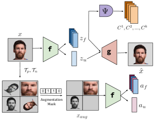
Figure 1: Overview of our architecture DisCont. Given a batch of images $x$, we generate an augmented batch $x_{aug}$ by sampling a set of stochastic transformations. We then encode $x$ and $x_{aug}$ to extract their latent representations $z_{f}$, $z_{u}$ and $a_{f}$, $a_{u}$ respectively. $z_{f}$ is then used to construct ‘Attribute Context Vectors’ $C^{1},C^{2},...,C^{k}$ corresponding to each feature attribute. The context vectors and the latent representations are then used to optimize our disentanglement objective.

2.2 Model Description

To enforce the learning of rich and disentangled attributes, we propose to view the underlying latent space as two disjoint subspaces.

• $Z_{f}\subset\mathbb{R}^{d\times k}$: denotes the feature attribute space containing the disentangled and interpretable attributes, where $d$ and $k$ denote the dimensionality of the space and the number of feature attributes respectively.

• $Z_{u}\subset\mathbb{R}^{d}$: denotes the unspecified attribute space containing background and miscellaneous attributes, where $d$ is the dimensionality of the space. We enforce a $\mathbf{\mathcal{N}(\boldsymbol{0},\boldsymbol{I})}$ prior over this space following (Mathieu et al., 2016) and (Jha et al., 2018).

Assume that we have an invertible encoding function $f$ parameterized by $\theta$, then each image $x$ can be encoded in the following way:

$$z_{f},z_{u}=f_{\theta}(x),z_{f}\in{Z_{f}},z_{u}\in Z_{u}$$

where, we can index $z_{f}$ to recover the independent feature attributes i.e. $z_{f}=[z_{f,1},z_{f,2},...,z_{f,k}]$. To project the latent encodings back to image space, we make use of a decoding function $g$ parameterized by $\phi$. Therefore, we can get image reconstructions using the separate latent encodings.

$$\hat{x}=g_{\phi}(z_{f},z_{u})$$

2.2.1 Composite Data Augmentations

Following our initial hypothesis of recovering latent attributes using stochastic transformations, we formulate a mask-based compositional augmentation approach that leverages positive and negative transformations.

Assume that we have two sets of stochastic transformations $\mathcal{T}_{p}=\{p_{1},p_{2},...,p_{k}\}$ and $\mathcal{T}_{n}=\{n_{1},n_{2},...,n_{k}\}$ that can augment an image into a correlated form i.e. $x_{aug}=t(x),t:\mathbb{R}^{C\times H\times W}\rightarrow\mathbb{R}^{C\times H\times W},t\in\mathcal{T}_{p}\cup\mathcal{T}_{n}$. $\mathcal{T}_{p}$ denotes the positive set of transformations that when applied to an image should not change any of the underlying attributes, whereas $\mathcal{T}_{n}$ denotes the negative set of transformations that when applied to an image should change a single underlying attribute, i.e., when $n_{i}$ is applied to an image $x$, it should lead to a change only in the $z_{f,i}$ attribute and all other attributes should be preserved.

For every batch of images $x=\{x_{1},x_{2}...x_{B}\}$, we sample a subset of transformations to apply compositionally to $x$ and retrieve an augmented batch $x_{aug}$ and a mask vector $m\in\{0,1\}^{k}$. This is further detailed in Appendix A and Appendix B.

2.2.2 Attribute Context Vectors

Taking inspiration from (van den Oord et al., 2018), we propose attribute context vectors $C^{i}{\color[rgb]{1,1,1}1}\forall i\in\{1,2,...,k\}$. A context vector $C^{i}$ is formed from each of the individual feature attributes $z_{f}^{i}$ through a non-linear projection. The idea is to encapsulate the batch invariant identity and variability of the $i_{th}$ attribute in $C^{i}$. Hence, each individual context vector should capture an independent disentangled feature space of the individual factors of variation. Assume a non-linear mapping function $\Psi:\mathbb{R}^{d\times B}\rightarrow\mathbb{R}^{c}$, where $c$ denotes the dimensionality of each context vector $C^{i}$ and $B$ denotes the size of a sampled mini-batch. We construct context vectors by aggregating all the $i^{th}$ feature attributes locally within the sampled minibatch.

$$C^{i}=\Psi\Big{(}[z_{f,1}^{i},z_{f,2}^{i},...,z_{f,B}^{i}]\Big{)}\forall i\in\{1,2,...,k\}$$

2.3 Loss Functions

We describe the losses that we use to enforce disentanglement and interpretability within our feature attribute space.
We have a reconstruction penalty term to ensure that $z_{u}$ and $z_{f}$ encode enough information in order to produce high-fidelity image reconstructions.

$$\mathcal{L}_{R}=\sum_{i=0}^{B}\left\lVert\hat{x}_{i}-x_{i}\right\rVert_{2}^{2}$$ (3)

To ensure that the unspecified attribute $z_{u}$ acts as a generative latent code that encodes the arbitrary features within an image, we enforce the ELBO KL objective (Kingma & Welling, 2013) on $z_{u}$.

$$\mathcal{L}_{KL}=KL\Big{(}f_{\theta}(z_{u}|x,z_{f})\|\mathcal{N}(\boldsymbol{0},\boldsymbol{I}))\Big{)}$$ (4)

where $KL(P\|Q)=\int_{-\infty}^{\infty}p(x)\log(\frac{p(x)}{q(x)})$, $p$ and $q$ are the densities of arbitrary continuous distributions $P$ and $Q$ respectively.

We additionally enforce clustering using center loss in the feature attribute space $Z_{f}$ by differentiating inter-attribute features. This metric learning training strategy (Wen et al., 2016) promotes accumulation of feature attributes into distantly-placed clusters by providing additional self-supervision in the form of pseudo-labels obtained from the context vectors.

The center loss enforces the increment of inter-attribute distances, furthermore, diminishing the intra-attribute distances. We make use of the $\Psi$ function to project the feature attributes into the context vector space and then apply the center loss given by Equation 5.

$$P_{j}^{i}=\Psi\Big{(}[z_{f,j}^{i},z_{f,j}^{i},...,z_{f,j}^{i}]\Big{)}$$

$$\forall i\in\{1,2,...,k\},j\in\{1,2,...,B\}$$

$$\mathcal{L}_{cen}=\frac{1}{2}\sum_{i=1}^{k}\sum_{j=1}^{B}||P_{j}^{i}-C^{i}||_{2}^{2}$$ (5)

where, context vectors $C^{i}$ function as centers for the clusters corresponding to the $i^{th}$ attribute.

We also ensure that the context vectors do not deviate largely across gradient updates, by imposing a gradient descent update on the context vectors.

$$C^{i}\leftarrow C^{i}-\eta\frac{\partial\mathcal{L}_{total}}{\partial C^{i}}$$

Finally, to ensure augmentation-specific consistency within the feature attributes, we propose a feature-wise regularization penalty $\mathcal{L}_{A}$. We first generate the augmented batch $X_{aug}$ and mask $m$ using Algorithm 1. We then encode $x_{aug}$ to produce augmented feature attributes $a_{f}$ and unspecified attribute $a_{u}$ in the following way:

$$a_{f},a_{u}=f_{\theta}(x_{aug})$$

Now, since we want to ensure that a specific negative augmentation $n_{i}$ enforces a change in only the $i_{th}$ feature attribute $z_{f}^{i}$, we encourage the representations of $a_{f}^{i}$ and $z_{f}^{i}$ to be close in representation space. Therefore, this enforces each feature attribute to be invariant to specific augmentation perturbations. Further, since the background attributes of images should be preserved irrespective of the augmentations applied, we also encourage the proximity of $z_{u}$ and $a_{u}$. This augmentation-consistency loss is defined as:

$$\mathcal{L}_{A}=\sum_{i=1}^{k}\Big{(}1-m[i]\Big{)}\left\lVert z_{f}^{i}-a_{f}^{i}\right\rVert^{2}_{2}+\left\lVert z_{u}-a_{u}\right\rVert^{2}_{2}$$ (6)

The overall loss of our model is a weighted sum of these constituent losses.

$$\mathcal{L}_{total}=\mathcal{L}_{R}+\lambda_{KL}\mathcal{L}_{KL}+\lambda_{cen}\mathcal{L}_{cen}+\mathcal{L}_{A}$$ (7)

where, weights $\lambda_{KL}$ and $\lambda_{cen}$ are treated as hyperparameters. Implementation details can be found in Appendix D.

3 Experiments

We employ a diverse set of four datasets to evaluate the efficacy of our approach , the details of which can be found in Appendix C.

3.1 Quantitative Results

Informativeness. To ensure a robust evaluation of our disentanglement models using unsupervised metrics, we compare informativeness scores (defined in (Do & Tran, 2020)) of our model’s latent chunks in Fig 2 with the state-of-the-art unsupervised disentanglement model presented in (Hu et al., 2018) (which we refer as MIX). A lower value of informativeness score suggests a better disentangled latent representation. Further details about the evaluation metric can be found in Appendix E.

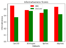
Figure 2: Informativeness scores for DisCont and MIX across datasets

3.2 Qualitative Results

Latent Visualization. We present latent visualisation for the test set samples with and without the unspecified chunk, i.e. $Z_{u}$. The separation between these latent chunks in the projected space manifests the decorrelation and independence between them. Here, we present latent visualisations for the dsprites dataset, the same for the other datasets can be found in Appendix G.

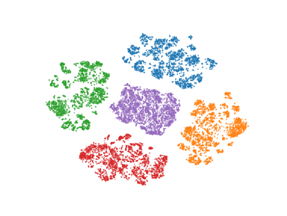
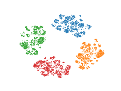
Figure 3: Latent space visualizations for dsprites dataset with all feature chunks (Top), i.e. $Z_{f}\cup Z_{u}$ and specified feature chunks (Bottom), i.e. $Z_{f}$. Each color depicts samples from different latent chunks, purple color representing the unspecified chunk, i.e. $Z_{u}$.

Attribute Transfer. We present attribute transfer visualizations to construe the quality of disentanglement. The images in the first two rows in each grid are randomly sampled from the test-set. The bottom row images are formed by swapping one specified attribute from the top row image with the corresponding attribute chunk in the second row image, keep all other attributes fixed. This allows us to quantify the purity of attribute-wise information captured by each latent chunk. We present these results for Cars3D and 3DShapes here, while the others in Appendix F.

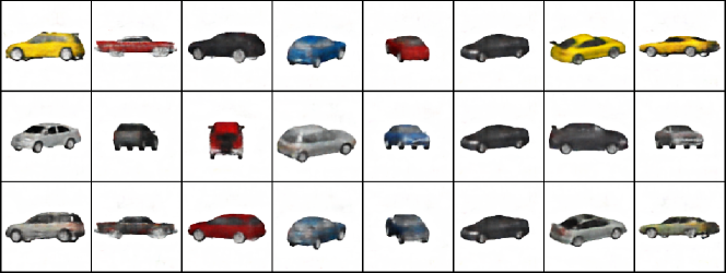
(a) Cars3D; Specified Attribute: Color

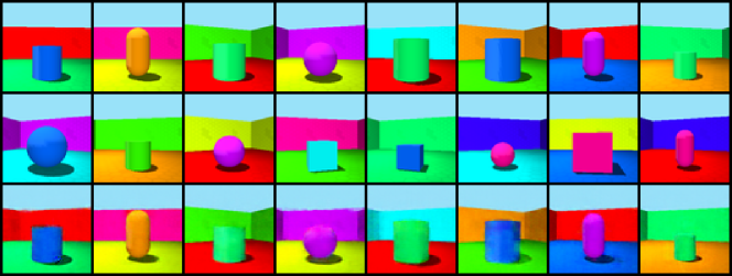
(b) 3DShapes; Specified Attribute: Orientation

Figure 4: Attribute transfer results obtained by swapping the specified chunk.

4 Conclusion

In this paper, we propose a self-supervised attribute disentanglement framework DisCont which leverages specific data augmentations to exploit the spatial inductive biases present in images. We also propose ‘Attribute Context Vectors’ that encapsulate the intra-attribute variations. Our results show that such a framework can be readily used to recover semantically meaningful attributes independently.

Appendix A Mask and Augmented Batch Generation Algorithm

This section describes the generation of the mask and the augmented batch for the computation of the augmentation-consistency loss $\mathcal{L}_{A}$ (refer Equation 6). The entire algorithm is detailed below:

Algorithm 1 Mask and Augmented Batch generation   Input: A batch of images $x$, the set of positive transformations $\mathcal{T}_{p}$, the set of negative transformations $\mathcal{T}_{n}$, number of feature attributes $k$   Output: The augmented batch $x_{aug}$, the mask $m$   Initialize $m=[0,0,...,0]_{k}$, $x_{aug}=x$   for $i=1$ to $k$ do      $p\sim Bernoulli(0.5)$      if $p=1$ then         $m[i]=1$         $x_{aug}=n_{i}(x_{aug})$      end if   end for   for $i=1$ to $k$ do      $p\sim Bernoulli(0.5)$      if $p=1$ then         $x_{aug}=p_{i}(x_{aug})$      end if   end for   return $x_{aug},m$

Appendix B Augmentations

The set of augmentations and their sampling range of parameters that we use in this work are detailed in the table below:

	Positive Augmentations $\mathcal{T}_{p}$
Type	Parameter	Range
Gaussian Noise	$\sigma$	[0.5, 1, 2, 5]
Gaussian Smoothing	$\sigma$	[0.1, 0.2, 0.5, 1]
	Negative Augmentations $\mathcal{T}_{n}$
Type	Parameter	Range
Grayscale Transform	–	–
Flipping	Orientation	[Horizontal, Vertical]
Rotation	$\theta$	[90°, 180°, 270°]
Crop & Resize	–	–
Cutout	Length	[5, 10, 15, 20]

Table 1: Set of augmentations used for training DisCont.

Appendix C Dataset Description

We use the following datasets to evaluate our model performance:

• Sprites (Reed et al., 2015) is a dataset of 480 unique animated caricatures (sprites) with essentially 6 factors of variations namely gender, hair type, body type, armor type, arm type and greaves type. The entire dataset consists of 143,040 images with 320, 80 and 80 characters in train, test and validation sets respectively.

• Cars3D (Reed et al., 2015) consists of a total of 17,568 images of synthetic cars with elevation, azimuth and object type varying in each image.

• 3DShapes (Burgess & Kim, 2018) is a dataset of 3D shapes generated using 6 independent factors of variations namely floor color, wall color, object color, scale, shape and orientation. It consists of a total of 480,000 images of 4 discrete 3D shapes.

• dSprites (Matthey et al., 2017) is a dataset consisting of 2D square, ellipse, and hearts with varying color, scale, rotation, x and y positions. In total, it consists of 737,280 gray-scale images.

Appendix D Implementation, Training and Hyperparameter Details

We use a single experimental setup across all our experiments. We implement all our models on an Nvidia GTX 1080 GPU using the PyTorch framework. Architectural details are provided in Table 2. The training hyperparameters used are listed in Table 3.

Encoder $f$	Decoder $g$	Context Network $\Psi$
Input: $\mathbb{R}^{64\times 64\times 3}$	Input: $\mathbb{R}^{(k+1)\times d}$	Input: $\mathbb{R}^{k\times d}$
Conv $4\times 4$, 64, ELU, stride 2, BN	FC, $(k+1)\times d$, 1024, ReLU, BN	FC, $k\times d$, 4096, ReLU
Conv $3\times 3$, 128, ELU, stride 2, BN	FC, 1024, 4068, ReLU, BN	FC, 4096, $k\times c$, ReLU
Conv $3\times 3$, 256, ELU, stride 2, BN	Deconv, $3\times 3$, 256, ReLU, stride 2, BN
Conv $3\times 3$, 512, ELU, stride 2, BN	Deconv, $3\times 3$, 128, ReLU, stride 2, BN
FC, 4608, 1024, ELU, BN	Deconv, $3\times 3$, 64, ReLU, stride 2, BN
FC, 1024, $(k+1)\times d$, ELU, BN	Deconv, $4\times 4$, 3, ReLU, stride 2, BN

Table 2: Architectures for encoder $f$, decoder $g$ and context network $\Psi$ for all experiments. Here, Conv denotes 2D convolution layer, Deconv denotes 2D transposed convolution layer, FC denotes fully connected layer, BN denotes batch normalisation layer.

Parameter	Value
Batch Size ($B$)	64
Latent Space Dimension ($d$)	32
Number of Feature Attributes ($k$)	2
Context Vector Dimension ($c$)	100
KL-Divergence Weight ($\lambda_{KL}$)	1
Augmentation-Consistency Loss Weight ($\lambda_{A}$)	0.2
Optimizer	Adam
Learning Rate ($\eta$)	1e-4
Adam: $\beta_{1}$	0.5
Adam: $\beta_{2}$	0.999
Training Epochs	250

Table 3: Training hyperparameters for DisCont common across all datasets.

Appendix E Informativeness Evaluation Metric

As detailed in (Do & Tran, 2020), disentangled representations need to have low mutual information with the base data distribution, since ideally each representation should capture atmost one attribute within the data. The informativeness of a representation $z_{f,i}$ w.r.t data $x$ is determined by computing the mutual information $\mathbb{I}(x,z_{f,i})$ using the following Equation:

$$\mathbb{I}(x,z_{f,i})=\int_{x}\int_{z_{f}}p_{\mathcal{D}}(x)f(z_{f,i}|x)\log\Bigg{(}\frac{f(z_{f,i}|x)}{f(z_{f,i})}\Bigg{)}\,dx\,dz_{f}$$ (8)

where $f(\cdot)$ depicts the encoding function, i.e., $f:\mathbb{R}^{C\times H\times W}\rightarrow\mathbb{R}^{d}$ and $\mathcal{D}$ depicts the dataset of all samples, such that $\mathcal{D}=\{x_{i}\}_{i=1}^{N}$. The informativeness metric helps us capture the amount of information encapsulated within each latent chunk with respect to the original image $x$. We compare our DisCont model with unsupervised disentanglement model proposed by (Hu et al., 2018). For training the model in (Hu et al., 2018), we use the following hyperparameter values.

Hyperparameter	Sprites	Cars3D	3DShapes	dSprites
Latent Space Dimension ($d$)	256	96	512	96
Number of Chunks	8	3	8	3
Dimension of Each Chunk	32	32	64	32
Optimizer	Adam	Adam	Adam	Adam
Learning Rate ($\eta$)	2e-4	2e-4	5e-5	2e-4
Adam: $\beta_{1}$	0.5	0.5	0.5	0.5
Adam: $\beta_{1}$	0.99	0.99	0.99	0.99
Training Epochs	100	200	200	150

Table 4: Training hyperparameters for the model in (Hu et al., 2018)

Appendix F Attribute Transfer

We present attribute transfer visualizations for validating our disentanglement performance. The first two rows depict the sampled batch of images from the test set while the bottom row depicts the images generated by swapping the specified attribute from the first row images with that of the second row images. The style transfer results for Sprites are shown in Fig 5. The feature swapping results for the dSprites dataset were not consistent probably because of the ambiguity induced by the color transformation in the feature attribute space, when applied to the single channeled images.

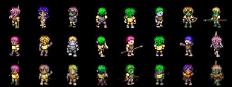
(a) Specified Attribute: Hair Color

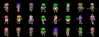
(b) Specified Attribute: Pose

Figure 5: Attribute transfer results for DisCont obtained by swapping the specified chunk.

Appendix G Latent Visualisation

In this section, we present the additional latent visualisations of the test set samples with and without the unspecified chunk, i.e., $Z_{u}$. The latent visualizations for the Cars3D, Sprites and 3DShapes datasets are shown in Fig 6.

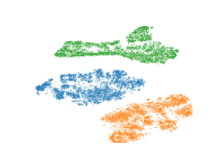
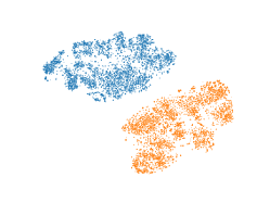
(a) Cars3D

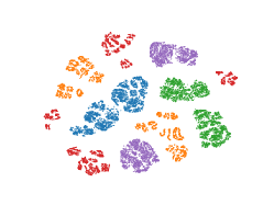
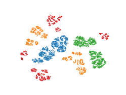
(b) 3DShapes

(c) Sprites

Figure 6: Latent space visualizations for Cars3D, 3DShapes and Sprites datasets with all feature chunks (Left) i.e., $Z_{f}\cup Z_{u}$ and specified feature chunks (Right) i.e., $Z_{f}$. Each color depicts samples from different latent chunks, green color representing the unspecified chunk, i.e., $Z_{u}$ for the Cars3D and Sprites dataset and purple for the 3DShapes dataset.

Appendix H Future Work

In the future, we would like to explore research directions that involve generalizing the set of augmentations used. Further as claimed in (Locatello et al., 2018), we would like to evaluate the performance gains of leveraging our disentanglement model in terms of sample complexity on various downstream tasks.

References

- Arora et al. (2019) Arora, S., Khandeparkar, H., Khodak, M., Plevrakis, O., and Saunshi, N. A theoretical analysis of contrastive unsupervised representation learning. arXiv preprint arXiv:1902.09229, 2019.
- Bengio (2013) Bengio, Y. Deep learning of representations: Looking forward. In International Conference on Statistical Language and Speech Processing, pp. 1–37. Springer, 2013.
- Bengio et al. (2013) Bengio, Y., Courville, A., and Vincent, P. Representation learning: A review and new perspectives. IEEE transactions on pattern analysis and machine intelligence, 35(8):1798–1828, 2013.
- Bhagat et al. (2020) Bhagat, S., Uppal, S., Yin, V. T., and Lim, N. Disentangling representations using gaussian processes in variational autoencoders for video prediction. ArXiv, abs/2001.02408, 2020.
- Burgess & Kim (2018) Burgess, C. and Kim, H. 3d shapes dataset. https://github.com/deepmind/3dshapes-dataset/, 2018.
- Cao et al. (2018) Cao, J., Katzir, O., Jiang, P., Lischinski, D., Cohen-Or, D., Tu, C., and Li, Y. Dida: Disentangled synthesis for domain adaptation. ArXiv, abs/1805.08019, 2018.
- Chen et al. (2020) Chen, T., Kornblith, S., Norouzi, M., and Hinton, G. A simple framework for contrastive learning of visual representations, 2020.
- Chen et al. (2018) Chen, T. Q., Li, X., Grosse, R. B., and Duvenaud, D. Isolating sources of disentanglement in variational autoencoders. In NeurIPS, 2018.
- Chen et al. (2016) Chen, X., Duan, Y., Houthooft, R., Schulman, J., Sutskever, I., and Abbeel, P. Infogan: Interpretable representation learning by information maximizing generative adversarial nets. In Advances in neural information processing systems, pp. 2172–2180, 2016.
- Cohen & Shashua (2016) Cohen, N. and Shashua, A. Inductive bias of deep convolutional networks through pooling geometry. arXiv preprint arXiv:1605.06743, 2016.
- Denton & Birodkar (2017) Denton, E. L. and Birodkar, V. Unsupervised learning of disentangled representations from video. In NIPS, 2017.
- Do & Tran (2020) Do, K. and Tran, T. Theory and evaluation metrics for learning disentangled representations. ArXiv, abs/1908.09961, 2020.
- Farhadi et al. (2009) Farhadi, A., Endres, I., Hoiem, D., and Forsyth, D. Describing objects by their attributes. In 2009 IEEE Conference on Computer Vision and Pattern Recognition, pp. 1778–1785, 2009.
- Ghosh & Gupta (2019) Ghosh, R. and Gupta, A. K. Investigating convolutional neural networks using spatial orderness. In Proceedings of the IEEE International Conference on Computer Vision Workshops, pp. 0–0, 2019.
- Gutmann & Hyvärinen (2010) Gutmann, M. and Hyvärinen, A. Noise-contrastive estimation: A new estimation principle for unnormalized statistical models. In Proceedings of the Thirteenth International Conference on Artificial Intelligence and Statistics, pp. 297–304, 2010.
- He et al. (2019) He, K., Fan, H., Wu, Y., Xie, S., and Girshick, R. Momentum contrast for unsupervised visual representation learning. arXiv preprint arXiv:1911.05722, 2019.
- Higgins et al. (2017) Higgins, I., Matthey, L., Pal, A., Burgess, C., Glorot, X., Botvinick, M. M., Mohamed, S., and Lerchner, A. beta-vae: Learning basic visual concepts with a constrained variational framework. In ICLR, 2017.
- Hsieh et al. (2018) Hsieh, J.-T., Liu, B., Huang, D.-A., Fei-Fei, L., and Niebles, J. C. Learning to decompose and disentangle representations for video prediction. In NeurIPS, 2018.
- Hu et al. (2018) Hu, Q., Szabó, A., Portenier, T., Zwicker, M., and Favaro, P. Disentangling factors of variation by mixing them. 2018 IEEE/CVF Conference on Computer Vision and Pattern Recognition, pp. 3399–3407, 2018.
- Hénaff et al. (2019) Hénaff, O. J., Srinivas, A., Fauw, J. D., Razavi, A., Doersch, C., Eslami, S. M. A., and van den Oord, A. Data-efficient image recognition with contrastive predictive coding, 2019.
- Jha et al. (2018) Jha, A. H., Anand, S., Singh, M. K., and Veeravasarapu, V. S. R. Disentangling factors of variation with cycle-consistent variational auto-encoders. ArXiv, abs/1804.10469, 2018.
- Kim & Mnih (2018) Kim, H. and Mnih, A. Disentangling by factorising. ArXiv, abs/1802.05983, 2018.
- Kim et al. (2019) Kim, M., Wang, Y., Sahu, P., and Pavlovic, V. Relevance factor vae: Learning and identifying disentangled factors. ArXiv, abs/1902.01568, 2019.
- Kingma & Welling (2013) Kingma, D. P. and Welling, M. Auto-encoding variational bayes. arXiv preprint arXiv:1312.6114, 2013.
- Kipf et al. (2019) Kipf, T., van der Pol, E., and Welling, M. Contrastive learning of structured world models. arXiv preprint arXiv:1911.12247, 2019.
- Le & Akoglu (2019) Le, T. and Akoglu, L. Contravis: contrastive and visual topic modeling for comparing document collections. In The World Wide Web Conference, pp. 928–938, 2019.
- Liu et al. (2015) Liu, Z., Luo, P., Wang, X., and Tang, X. Deep learning face attributes in the wild. In Proceedings of International Conference on Computer Vision (ICCV), December 2015.
- Locatello et al. (2018) Locatello, F., Bauer, S., Lucic, M., Rätsch, G., Gelly, S., Schölkopf, B., and Bachem, O. Challenging common assumptions in the unsupervised learning of disentangled representations. arXiv preprint arXiv:1811.12359, 2018.
- Ma et al. (2019) Ma, J., Zhou, C., Cui, P., Yang, H., and Zhu, W. Learning disentangled representations for recommendation. In NeurIPS, 2019.
- Mathieu et al. (2016) Mathieu, M., Zhao, J. J., Sprechmann, P., Ramesh, A., and LeCun, Y. Disentangling factors of variation in deep representation using adversarial training. ArXiv, abs/1611.03383, 2016.
- Matthey et al. (2017) Matthey, L., Higgins, I., Hassabis, D., and Lerchner, A. dsprites: Disentanglement testing sprites dataset. https://github.com/deepmind/dsprites-dataset/, 2017.
- Meng et al. (2019) Meng, Q., Pawlowski, N., Rueckert, D., and Kainz, B. Representation disentanglement for multi-task learning with application to fetal ultrasound. In SUSI/PIPPI@MICCAI, 2019.
- Misra & van der Maaten (2019) Misra, I. and van der Maaten, L. Self-supervised learning of pretext-invariant representations. arXiv preprint arXiv:1912.01991, 2019.
- Patrick et al. (2020) Patrick, M., Asano, Y. M., Fong, R., Henriques, J. F., Zweig, G., and Vedaldi, A. Multi-modal self-supervision from generalized data transformations. arXiv preprint arXiv:2003.04298, 2020.
- Peters et al. (2017) Peters, J., Janzing, D., and Schölkopf, B. Elements of causal inference: foundations and learning algorithms. MIT press, 2017.
- Reed et al. (2015) Reed, S. E., Zhang, Y., Zhang, Y., and Lee, H. Deep visual analogy-making. In NIPS, 2015.
- Schölkopf et al. (2012) Schölkopf, B., Janzing, D., Peters, J., Sgouritsa, E., Zhang, K., and Mooij, J. On causal and anticausal learning. arXiv preprint arXiv:1206.6471, 2012.
- Shi et al. (2019) Shi, J., Liang, C., Hou, L., Li, J., Liu, Z., and Zhang, H. Deepchannel: Salience estimation by contrastive learning for extractive document summarization. In Proceedings of the AAAI Conference on Artificial Intelligence, volume 33, pp. 6999–7006, 2019.
- Shukla et al. (2019) Shukla, A., Bhagat, S., Uppal, S., Anand, S., and Turaga, P. K. Product of orthogonal spheres parameterization for disentangled representation learning. In BMVC, 2019.
- Srinivas et al. (2020) Srinivas, A., Laskin, M., and Abbeel, P. Curl: Contrastive unsupervised representations for reinforcement learning. arXiv preprint arXiv:2004.04136, 2020.
- Tian et al. (2019) Tian, Y., Krishnan, D., and Isola, P. Contrastive multiview coding, 2019.
- Udandarao et al. (2020) Udandarao, V., Maiti, A., Srivatsav, D., Vyalla, S. R., Yin, Y., and Shah, R. R. Cobra: Contrastive bi-modal representation algorithm. arXiv preprint arXiv:2005.03687, 2020.
- van den Oord et al. (2018) van den Oord, A., Li, Y., and Vinyals, O. Representation learning with contrastive predictive coding, 2018.
- Villegas et al. (2017) Villegas, R., Yang, J., Hong, S., Lin, X., and Lee, H. Decomposing motion and content for natural video sequence prediction. ArXiv, abs/1706.08033, 2017.
- Vu & Huang (2019) Vu, H. T. and Huang, C.-C. Domain adaptation meets disentangled representation learning and style transfer. 2019 IEEE International Conference on Systems, Man and Cybernetics (SMC), pp. 2998–3005, 2019.
- Wen et al. (2016) Wen, Y., Zhang, K., Li, Z., and Qiao, Y. A discriminative feature learning approach for deep face recognition. In European conference on computer vision, pp. 499–515. Springer, 2016.
- Yang et al. (2019) Yang, J., Dvornek, N. C., Zhang, F., Chapiro, J., Lin, M., and Duncan, J. S. Unsupervised domain adaptation via disentangled representations: Application to cross-modality liver segmentation. MICCAI, 11765:255–263, 2019.
- Zhang et al. (2019) Zhang, J., Huang, Y., Li, Y., Zhao, W., and Zhang, L. Multi-attribute transfer via disentangled representation. In Proceedings of the AAAI Conference on Artificial Intelligence, volume 33, pp. 9195–9202, 2019.