Speech Fusion to Face: Bridging the Gap Between Human’s Vocal Characteristics and Facial Imaging

Abstract

While deep learning technologies are now capable of generating realistic images confusing humans, the research efforts are turning to the synthesis of images for more concrete and application-specific purposes. Facial image generation based on vocal characteristics from speech is one of such important yet challenging tasks. It is the key enabler to influential use cases of image generation, especially for business in public security and entertainment. Existing solutions to the problem of speech2face renders limited image quality and fails to preserve facial similarity due to the lack of quality dataset for training and appropriate integration of vocal features. In this paper, we investigate these key technical challenges and propose Speech Fusion to Face, or SF2F in short, attempting to address the issue of facial image quality and the poor connection between vocal feature domain and modern image generation models. By adopting new strategies on data model and training, we demonstrate dramatic performance boost over state-of-the-art solution, by doubling the recall of individual identity, and lifting the quality score from 15 to 19 based on the mutual information score with VGGFace classifier.

1 Introduction

Driven by the explosive growth of deep learning technologies, choi2018stargan ; choi2019stargan ; karras2019style , computer vision algorithms are now capable of generating high-fidelity images, such that humans can hardly distinguish real images from synthesized ones. Researchers in computer vision and other areas are seeking concrete applications to fully unleash the power of image synthesis. One of the most promising applications is the automatic generation of facial images based on the vocal characteristics extracted from human speech Oh_2019_CVPR ; wen2019face , referred to as speech2face in the rest of the paper. It is believed to be the key enabler to new business opportunities in public security, entertainment, and other industries. Specifically, given an audio clip containing the speech from a target individual, the speech2face system is expected to visualize the individual’s facial image, based on the voice of the target individual only.

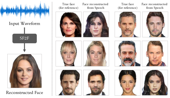
Figure 1: Left: The task of reconstructing the face image of an identity from his/her speech waveform. Right: A few $128\times 128$ sample images produced by our SF2F model, where human speech is the only input to the model. The groundtruth faces are shown for reference.

It is straightforward to understand vocal characteristics reflect important personal features, such as gender and age, which can be easily inferred over an individual’s speech. Existing studies have also demonstrated interesting observations on the presence of additional physical features of human face, strongly correlated to the vocal features in the voice. Unfortunately, the quality of the output facial images from these studies remains far from satisfactory, due to the following technical limitations. Firstly, the poor quality of paired dataset of individuals’ facial image and clean speech hinders the effective training of generative model for speech2face. Secondly, the integration of vocal features into state-of-the-art image synthesis models does not fully utilize the rich information from the speech of the individuals.

To address these technical challenges, we propose speech fusion to face, or SF2F in short, in this paper. Fig. 1 shows sample results of our method. We attempt to improve on top of the existing approaches in two general directions. To tackle the problem of poor data quality, we enhance the VoxCeleb dataset chung2018voxceleb2 ; nagrani2017voxceleb by filtering and rebuilding the face images of the celebrities. In Fig. 2, we present example images from filtered VGGFace dataset used in parkhi2015deep and our refined face image dataset. Common problems associated with the original face images from VGGFace dataset include (1) plenty of monolithic photos containing limited details of the faces; (2) the shooting angle and facial expression are highly diverse and technically difficult to normalize; (3) the background of the face image is not appropriately eliminated. Given these problems, we target to rebuild a high-quality face database for individuals in VoxCeleb database. By carefully retrieving images of these celebrities from the Internet and filtering with specific conditions, we generate HQ-VoxCeleb database with example figures shown in Fig. 2, with highly normalized facial images on different aspects.

Existing studies on speaker recognition, e.g., wan2018generalized , imply that vocal characteristics are highly unstable in the speech. Speaker recognition/verification algorithms usually extract short-time vocal features from speech and combine these features for final decision making. Such strategies cannot be directly copied to the solution for speech2face system because simple aggregation may lose some key information only available in certain pronunciations. In order to exploit the short-term features for face image generation, we introduce a new fusion strategy over speech extraction algorithms, which applies merging over the face images with different embeddings instead of the original embeddings. A new training scheme, with a new combination of loss functions, is introduced accordingly in order to maximize the information flowing from speech domain to facial imaging domain.

The key contributions of the paper are summarized as follows: (1) we introduce an enhanced face image dataset based on VoxCeleb, containing over 3,000 individual identities with high-quality front face images; (2) we present a new fusion strategy over the short-term vocal characteristics to stabilize the facial features for the synthetic image generation; (3) we propose a new loss function for the neural generative model in order to better preserve the vocal features in the facial generation process; (4) we evaluate the performance of the proposed model on both image fidelity and facial similarity to ground-truth and validates the performance gain over the state-of-the-art solutions.

2 Related Work

Generative Models. Plenty of generative frameworks have been proposed in recent years. Auto-regressive approaches such as PixelCNN and PixelRNN oord2016pixel generate images pixel by pixel, modeling the conditional probability distribution of sequences of pixels. Variational Autoencoders (VAEs) kingma2013auto ; NIPS2016_6528 jointly optimize a pair of encoder and decoder. The encoder transforms the input into a latent distribution, and the decoder synthesizes images based on the latent distribution. Remarkably, Generative Adversarial Networks (GANs) NIPS2014_5423 ; radford2015unsupervised which adversarially train a pair of generator and discriminator, have achieved the best visual quality.

Visual generation from audio. The generation of visual information from various types of audio signals has been studied extensively. There exist approaches taylor2017deep ; karras2017audio ; suwajanakorn2017synthesizing to generate an animation that synchronizes to input speech by mappings from phoneme label input sequences to mouth movements. Regarding pixel-level generation, Sadoughi and Busso’s approach sadoughi2019speech synthesizes talking lips from speech, and X2Face model wiles2018x2face manipulates the pose and expression of conditioning on an input face and audio. Wav2Pix model giro2019wav2pix is most relevant to our work, in the sense that it generates face images from speech, with the help of adversarial training. Their objective is to reconstruct the face texture of the speaker including expression and pose. In this paper, our objective is different, targeting to reconstruct a frontal face with a neutral expression, such that most facial attributes of the groundtruth are preserved.

Face-speech association learning. The associations between faces and speech have been widely studied in recent years. Cross-modal matching methods by classification shon2019noise ; nagrani2018learnable ; nagrani2018seeing ; wen2018disjoint and metric learning kim2018learning ; horiguchi2018face are adopted in identity verification and retrieval. Cross-modal features extracted from faces and speech are applied to disambiguate voiced and unvoiced consonants chung2017lip ; ngiam2011multimodal ; to track active speakers of a video hoover2017putting ; gebru2015tracking ; or to predict emotion albanie2018emotion and lip motions ngiam2011multimodal ; andrew2013deep from speech.

Face reconstruction from speech. Speech2face is an emerging topic in computer vision and machine learning, aiming to reconstruct face images from a voice signal based on existing sample pairs of speech and face images. Oh et al. Oh_2019_CVPR propose to use a voice encoder that predicts the face recognition embedding, and decode the face image using a pre-trained face decoder Cole_2017_CVPR . As the most similar approach to ours, Wen et al. wen2019face employ an end-to-end encoder-decoder model together with GAN framework, based on filtered VGGFace dataset parkhi2015deep . In this paper, we propose a suite of new approaches and strategies to improve the quality of face images on top of these studies.

3 Data Quality Enhancement

As demonstrated in Fig. 2, the poor quality of training dataset for speech2face is one of the major factors hindering the improvement of speech2face performance. To eliminate the negative impact of the training dataset, we carefully design and build a new high-quality face database on top of VoxCeleb dataset chung2018voxceleb2 ; nagrani2017voxceleb , such that face images associated with the celebrities are all at reasonable quality. To fulfill the vision of data quality, we set a number of general guidelines over the face images as the underlying measurement on quality, covering attributes including face angles, lighting conditions, facial expressions, and image background. In order to fully meet the standards as listed above, we adopt a data processing pipeline to build the enhanced HQ-VoxCeleb dataset for our speech2face model training, with details available in Appendix B.1. In Table 1, we summarize the statistics of the result dataset after the adoption of the processing steps above. In Appendix B.1, we compare HQ-VoxCeleb with existing audiovisual datasets, to justify HQ-VoxCeleb is the most suitable dataset for end-to-end learning of speech2face algorithms. HQ-VoxCeleb dataset will be released later.

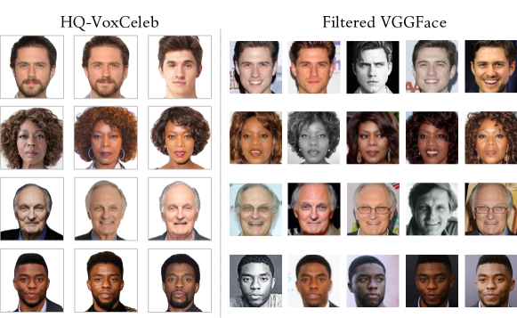
Figure 2: The quality variance of the original manually filtered VGGFace dataset (on the right of the figure) parkhi2015deep diverts the efforts of face generator model to the normalization of the faces. By filtering and correcting the face database (on the left), the machine learning models could focus more on linking facial and vocal features.

Table 1: Statistics of HQ-VoxCeleb dataset, where speech data is acquired from the identity intersection with VoxCeleb dataset.

Attribute	Total	Train. Set	Val. Set	Test Set
#Identity	3,638	2,890	370	378
#Image	8,028	6,375	859	794
#Speech	609,700	478,009	63,337	68,354
Avg. Reso.	505.41$\times$505.41	505.78$\times$505.78	503.63$\times$503.63	504.37$\times$504.37

4 Model and Approaches

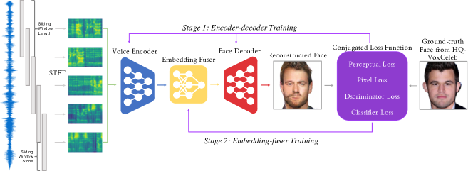
Figure 3: Overview of the framework of our proposed SF2F

The overall architecture of our proposed SF2F model is illustrated in Fig. 3. The pipeline of our model follows the popular encoder-decoder architecture used in most of the generative models. We refine the structure to make a better fit for the speech2face task. At inference, we apply a rolling window over the input speech audio. Each window is regarded as an individual local speech segment and the corresponding features from one segment are extracted and stored in a 1D vector by a speech encoder. The global facial features are generated by applying an attention fuser over the sequence of local facial features from the sliding windows. As shown in Fig. 3, the whole training procedure consists of two stages. In the first stage, the voice encoder and face decoder are first optimized to correlate facial features with vocal features extracted from short-time audio windows ranging from 1 second to 1.5 seconds and reconstructing faces based on the features. In the second stage, longer range of audio (global audio) ranging from 6 seconds to 25 seconds are converted into a series of local audio segments with a sliding window; the voice encoder converts the audio segments into corresponding embeddings. An embedding fuser follows to obtain a global facial embedding conditioned on the sequence of local facial embeddings. The weights of voice encoder and face decoder remain fixed in the second stage, while the two training stages share the same conjugated loss function. On the other hand, our approach enables the model to save efforts on learning useless variations mostly contained in long audios, such as the prosody of the speaker and linguistic features of the transcript, and consequently prevents the model from over-fitting. Moreover, the proposed framework maximizes the information extraction from short audios containing most important vocal features with matching features in the facial imaging domain.

Pre-Processing. Over every speech audio waveform, we apply a sliding window at fixed width of 1.25 seconds with 50% overlap. Short-time Fourier Transform (STFT) muller2015fundamentals computes the mel-spectrogram of each window. The input waveform is thus converted into a sequence of mel-spectrograms $M=\left\{m_{i}\in\mathbb{R}^{{T}\times{F}}\right\}$, where $T$ denotes the number of frames in the time domain, and $F$ denotes frequency. As we use an end-to-end training pipeline, instead of relying on pre-trained face decoder as in Oh_2019_CVPR , we expect the groundtruth face images to contain least irrelevant variations, including pose, lighting, and expression. This is enforced by our data enhancement scheme in Section 3. Specifically, each groundtruth face image is denoted by $I\in\mathbb{R}^{3\times{H}\times{W}}$ in the rest of the paper.

Voice Encoder. We use a 1D CNN composed of several 1D Inception modules szegedy2015going to process mel-spectrogram. The voice encoder module converts each short input speech segment into a predicted facial feature embedding. The architecture of the 1D Inception module and the voice encoder is described with details in Appendix D. The encoder’s basic building block is a 1D Inception module, where each Inception module consists of four parallel 1D CNNs, each with kernel size ranging from 2 to 7 and stride 2 with convolution along the time domain, followed by ReLU activation and batch normalization ioffe2015batch . The Inception module models various ranges of short-term mel-spectrogram dependency, and enables more accurate information flow from voice domain to image domain, compared to plain single-kernel-size CNN used in wen2019face . The number of channels grows from lower layers to higher layers in the stack, in order to reflect the bandwidth of the frequency domain to the corresponding layers. On top of the stack of basic building blocks, an average pooling layer outputs a predicted facial embedding $e_{i}\in\mathbb{R}^{d}$ for each mel-spectrogram segment $m_{i}$. The embedding $e_{i}$ is normalized as $e_{i}=\frac{e_{i}}{\max(\lVert e_{i}\rVert_{2},\epsilon)}$, in which $\epsilon=10^{-12}$ by default.

Face Decoder. The decoder reconstructs target individual’s face image based on embeddings from the individual’s speech segments. Since HQ-VoxCeleb dataset eliminates unnecessary and redundant variance on irrelevant features, the face decoder is expected to target the most distinctive features of faces. The basic building blocks of our face decoder include a 2D bilinear upsampling operator, a 4$\times$4 convolution operator, a ReLU activation, and a batch normalization. On top of stacked basic building blocks, a 1$\times$1 convolution with linear activation is deployed to generate the output $I^{\prime}$.

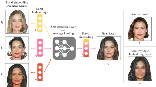
Figure 4: Demonstration of the functionality of embedding fuser. In this case, three local embeddings $\{e_{1},e_{2},e_{3}\}$ are fused into global embedding $f$. Faces $\{I_{1},I_{2}\}$ decoded from embeddings $\{e_{1},e_{2}\}$ contains obvious visual defects due to the noises in the corresponding audio segments. Face $I_{3}$ renders better image quality, while the face shape and skin color is not even close to the ground truth. By fusing $\{e_{1},e_{2},e_{3}\}$ into $f$, the face decoder outputs $I_{f}$ combining the merits of $\{I_{1},I_{2},I_{3}\}$ and avoid the local defects within $\{I_{1},I_{2},I_{3}\}$. Without embedding fuser, the result image can hardly distinguish the appropriate features for the face generation procedure.

Embedding Fuser. The most important part of our model is the fuser of the embeddings from the speech segments. The rationale behind the independent extraction of local features from the speech segment is to enable the model to focus on the vocal characteristics of the individual. When the voice encoder is directly applied to long speech audio, for example, the output features may contain features over the texts in the speech, as well as prosodic features on the emotion and presentation style of the speakers. These features are speaker-independent and therefore irrelevant to the features of the individuals in facial imaging domain. However, embeddings from speech segments are not stable by themselves. Because of the variance of text content in the speech segment, each embedding may reflect completely different vocal characteristics useful to the speech2face task. The embedding fuser is illustrated in the example in Fig. 4.

Given a sequence of mel-spectrograms $M=\{m_{1},m_{2},...,m_{T-1},m_{T}\}$ generated Short-Time Fourier Transform (STFT) over $T$ consecutive speech segments, voice encoder transforms $M$ into a sequence of embedding vectors $E_{1:T}=\{e_{1},e_{2},...,e_{T-1},e_{T}\}$, each of which contains certain vocal features correlated to different facial features. In order to preserve the useful information from all of the embeddings, embedding fuser first processes $E_{1:T}$ with a self-attention layer. Given a voice embedding vector $e_{i}$, its attention score to another voice embedding vector $e_{j}$ is calculated by $s(e_{i},e_{j})=e_{i}^{T}W_{a}e_{j}$. Based on the scores between the embedding vectors, $\beta_{i,j}$ indicates the degree of $e_{i}$ attending to $e_{j}$, measured by $\beta_{i,j}=\frac{\exp(s(e_{i},e_{j}))}{\sum{{}_{j=1}^{N}}\exp(s(e_{i},e_{j}))}$. The output of $e_{i}$, for each $1\leq i\leq T$, attending to the whole sequence $E$ is finalized as $a_{i}=\sum{{}_{j=1}^{T}}\beta_{i,j}e_{j}$. Here, attention output $a_{i}$ is concatenated with voice embedding vector $e_{i}$ and then goes through a linear transformation, generating the output of a fine-grained feature $f_{i}=W_{f}[a_{i},e_{i}]+b_{f}$. Finally, average pooling is performed along the time dimension, $f=\frac{1}{T}\sum{{}_{i=1}^{T}}f_{i}$, where $f$ is the globally fused embedding vector, with dimensionality identical to $e_{i}$ and $f_{i}$.

Discriminators. To improve the generative capability of our proposal, two discriminators, namely $D_{real}$ and $D_{id}$, are employed as the adversary to the generative model. The discriminator $D_{real}$ is the traditional binary discriminator as introduced in standard Generative Adversarial Network (GAN) NIPS2014_5423 that distinguishes the synthesized images from the real images, by optimizing over the following objective function: $\mathcal{L}_{G}=\mathop{\mathbb{E}}\limits_{x\sim p_{\mathrm{real}}}\log D_{real}(x)+\mathop{\mathbb{E}}\limits_{x\sim p_{\mathrm{fake}}}\log(1-D_{real}(x))$, where $x\sim p_{\mathrm{real}}$ and $x\sim p_{\mathrm{fake}}$ represent the distributions of real and synthesized images, respectively. Instead of telling difference between real and fake images, the discriminator $D_{id}$ attempts to classify the images into the identity of the individual in the image. A standard identity classifier aims to optimize the following objective function: $\mathcal{L}_{id}=\mathop{\mathbb{E}}\limits_{x\sim p_{\mathrm{real}}}\sum_{i=1}^{C}y_{i}\log(D_{id}(x)_{i})$.

Conditioned on human speech, the generator network is expected to synthesize human face images, which can be correctly classified by $D_{id}$. This is achieved by minimizing the objective function $\mathcal{L}_{C}=\mathop{\mathbb{E}}\limits_{x\sim p_{\mathrm{fake}}}\sum_{i=1}^{C}-y_{i}\log(D_{id}(x)_{i})$ on generated images .

Training Scheme. As shown in Fig. 3, the weights associated with the encoder-decoder and the embedding fuser are updated in two stages, respectively. The unified conjugated loss function consists of four different types of losses:

(1) Image Reconstruction Loss. $\mathcal{L}{{}_{1}}=\lVert I-\hat{I}\rVert{{}_{1}}$ penalizes the $L_{1}$ differences between the ground-truth image $I$ and the reconstructed image $\hat{I}$. (2) Adversarial Loss. Image adversarial loss $\mathcal{L}_{G}$ from $D_{real}$ encourages generated face image to appear photo-realistic; (3) Auxiliary Classifier Loss. $\mathcal{L}_{C}$ ensures generated objects to be recognizable and well-classified by $D_{id}$; (4) FaceNet Perceptual Loss. Image perceptual loss $\mathcal{L}_{P}$ penalizes the $L_{1}$ difference in the global feature space between the ground truth image $I$ and the reconstructed image $\hat{I}$, while object perceptual loss. Inspired by johnson2016perceptual , we add a lightweight perceptual loss between generated images and ground truth images to keep the perceptual similarity. This loss not only improves the quality of the generated images, but also enhances the similarity of the output images to the ground truth faces. The loss function of our model is finally formulated as, $\mathcal{L}_{conj}=\lambda_{1}\mathcal{L}{{}_{1}}+\lambda_{2}\mathcal{L}_{G}+\lambda_{3}\mathcal{L}_{C}+\lambda_{4}\mathcal{L}_{P}$, where $\{\lambda_{1},\lambda_{2},\lambda_{3},\lambda_{4}\}$ are the hyper-parameters used to balance the loss functions.

5 Experiments

Implementation Details. We train all our SF2F models using Adam optimizer dpk2015adam with learning rate 5e-4 and batch size 256; the encoder-decoder training takes 120,000 iterations, and the fuser training takes 360 iterations. $\lambda_{1}$, $\lambda_{2}$, $\lambda_{3}$, $\lambda_{4}$ are set at 10, 1, 0.05 and 100, respectively. We implement discriminator with ReLU activation and batch normalization. More information of the dataset is covered in Section 3.

Metric on Similarity. We evaluate the quality of synthesis outputs by measuring the perceptual similarity between the reconstructed face and its corresponding groundtruth Oh_2019_CVPR . By feeding the generated face image to a pre-trained FaceNet schroff2015facenet , we generate the face embedding by retrieving the output of the last layer prior to softmax. Given the embeddings from the groundtruth, denoted by $U=\{u_{1},u_{2},\ldots,u_{N}\}$, and the embeddings from the synthesized images, denoted by $U^{\prime}=\{u^{\prime}_{1},u^{\prime}_{2},\ldots,u^{\prime}_{N}\}$, over $N$ individuals in our test dataset, we calculate and report the average cosine similarity, i.e., $\sum^{N}_{i=1}\cos(u_{i},u^{\prime}_{i})/N$, and the average $L_{1}$ distance, i.e., $\sum^{N}_{i=1}\|u_{i}-u^{\prime}_{i}\|/N$.

Metric on Retrieval Performance. We also validate the usefulness of the output face images by querying the test face dataset with the generated face as the reference image, aiming to retrieve the identity of the speaker Oh_2019_CVPR . Specifically, Recall@K with $K=1,2,5,10$ are reported, which is the ratio of query face images with its groundtruth identity included in the top-$K$ similar faces.

Image Quality Evaluation. Existing studies Oh_2019_CVPR ; wen2019face do not report the general quality of the generated face images, partly because of the missing of appropriate metric on face image synthesis quality. While Inception Score salimans2016improved is commonly employed in studies of image generation johnson2018image ; xu2018attngan ; yikang2019pastegan ; zhang2017stackgan , it is designed to cover a wide variety of object types in the images. We introduce and report a new quality metric based on VGGFace classifier, which is calculated in a similar way as Inception Score. Inception classifier is simply replaced with VGGFace classifier. The mutual information based on the probabilities over the identities, i.e., $\mathbf{VFS}(G)=\exp\bigg{(}\frac{1}{N}\sum_{i=1}^{N}D_{KL}\Big{(}p(y|\mathbf{x}^{(i)})||p(y)\Big{)}\bigg{)}$, is used to measure image quality. Here, $\mathbf{x}^{(i)}$ stands for the $i$-th image synthesized by the generator $G$, $y$ is the prediction by VGGFace, and $D_{KL}$ denotes KL Divergence. To justify the adoption of VGGFace Score, we compare it against Inception Score over the real images in HQ-VoxCeleb dataset, at different resolutions. The results in table 2 show that Inception Scores are locked in a small range between 2.0 and 2.6 regardless of the image resolution, implying the total information of the real faces could be encoded with 1 bit only! This is because Inception V3 is not designed for face classification and thus skips the variance of the details on the faces. VGGFace Score, on the other hand, demonstrates a much more reasonable evaluation of face image quality.

Table 2: VGGFace and Inception Scores on face images at different resolutions in HQ-VoxCeleb

Resolution	64 $\times$ 64	128 $\times$ 128	256 $\times$ 256
Inception Score	2.074 $\pm$ 0.067	2.286 $\pm$ 0.036	2.583 $\pm$ 0.108
VGGFace Score	48.720 $\pm$ 1.688	51.048 $\pm$ 3.633	50.525 $\pm$ 1.862

Comparison with existing work. We include voice2face wen2019face as the state-of-the-art baseline in this group of experiments. To make a fair comparison, we implement voice2face by ourselves and train its model with our HQ-VoxCeleb dataset. Both voice2face and our SF2F are trained to generate images with 64$\times$64 pixels, and evaluated with 1.25 seconds and 5 seconds of human speech clips. As is presented in Table 3, SF2F outperforms voice2face by a large margin on all metrics. By deploying fuser in SF2F, the maximal recall@10 reaches 36.65%, almost doubling the recall@10 of voice2face at 20.82. Performance comparison on filtered VGGFace dataset is discussed in Appendix C.2.

Table 3: Performance on HQ-VoxCeleb in feature similarity, retrieval recall@K, and VGGFace Score

Setting		Similarity		Retrieval				Quality
Method	Len.	cosine	L1	R@1	R@2	R@5	R@10	VFS
random	-	-	-	1.00	2.00	5.00	10.00	-
voice2face	1.25 sec	0.202	23.46	1.77	3.55	14.60	20.33	15.47 $\pm$ 0.67
SF2F (no fuser)	1.25 sec	0.304	19.22	5.32	8.10	19.27	32.80	18.59 $\pm$ 0.87
voice2face	5 sec	0.205	23.17	1.64	3.64	15.12	20.82	15.68 $\pm$ 0.64
SF2F (no fuser)	5 sec	0.294	18.51	4.11	8.38	19.43	33.97	18.54 $\pm$ 1.02
SF2F	5 sec	0.317	17.91	5.75	9.32	20.36	36.65	19.49 $\pm$ 0.59

Effect of input audio length. We examine different audio length for the extraction of vocal features. It is crucial to capture the most important vocal features while reserving minimal irrelevant linguistic and prosody information from speech. In Table 4, the results show speech audios between 1 second and 1.5 seconds achieve the best performance on most of the feature similarity and retrieval recall metrics. This justifies the assumption that only short audio’s vocal characteristics are useful to the face reconstruction task. VFS remains stable with different audio lengths, implying the capacity of the information flow from vocal domain to facial domain is fairly static.

Table 4: Performance of SF2F (no fuser) on HQ-VoxCeleb, with audios limited to different lengths.

Setting	Similarity		Retrieval				Quality
Audio Length	cosine	L1	R@1	R@2	R@5	R@10	VFS
0.5 - 1 sec	0.230	21.85	4.67	8.38	15.40	26.05	18.17 $\pm$ 0.75
1 - 1.5 sec	0.296	18.51	5.02	8.60	19.43	32.25	18.53 $\pm$ 0.72
1.5 - 3 sec	0.294	18.79	4.96	8.78	18.59	29.88	18.67 $\pm$ 1.72
3 - 6 sec	0.274	19.21	4.33	8.43	17.10	30.14	18.05 $\pm$ 1.14
6 - 10 sec	0.227	21.92	3.34	6.58	14.73	26.92	18.40 $\pm$ 2.03

Figure 5: Examples of 64 $\times$ 64 generated images using SF2F and voice2face

Effect of output resolution. SF2F is also trained to generate large images with 128$\times$128 pixels. Two different approaches are tested over higher resolution, including a single-resolution SF2F model optimized to generate 128$\times$128 pixels only, and a multi-resolution model optimized to generate both 64$\times$64 pixels and 128$\times$128 pixels. Both of the solutions are equipped with the same conjugated loss function. Table 5 compares the performance of SF2F with fusers trained under different schemes with speech length at 5 seconds. Single resolution model performs worse than the other two, suffering from the unstable optimization gradient over a deeper face decoder. Multi-resolution model achieves comparable performance to single-resolution model. This is because most of the speaker-dependent facial features are already included in 64$\times$64 pixels. The addition of more details with higher resolution does not benefit at all.

Table 5: Performance of SF2F on HQ-VoxCeleb, with image data resized to different resolution

Setting		Similarity		Retrieval				Quality
Optimization	Resolution	cosine	L1	R@1	R@2	R@5	R@10	VFS
single-reso.	64 $\times$ 64	0.317	17.91	5.75	9.32	20.36	36.65	19.49 $\pm$ 0.59
single-reso.	128 $\times$ 128	0.278	18.54	5.02	8.60	19.43	32.25	18.53 $\pm$ 1.75
multi-reso.	128 $\times$ 128	0.313	17.46	6.10	9.25	18.77	35.38	20.10 $\pm$ 0.47

Qualitative results. We also directly compare the visual performance of the generated face images from SF2F and voice2face. We compare SF2F and voice2face trained on HQ-VoxCeleb, to justify the performance boost brought by our model design. We also provide results generated by voice2face pre-trained and released by Wen et al. v2f_github , to prove the improvement brought by HQ-VoxCeleb. All of the images, from all three of the models, are reconstructed based on speech ranging from 4-7 seconds. As shown in Fig. 5, faces reconstructed by SF2F contain obviously preserves more accurate and meaningful facial features. The pose, expression, and lighting over the faces from SF2F are generally more stable and consistent. More qualitative results of 128 $\times$ 128 face image generation are available in Appendix A.

Ablation study. Ablation experiments are discussed in Appendix C.1.

6 Conclusion and Future Work

In this paper, we present Speech Fusion to Face (SF2F), a new strategy of building generative models converting speech into vivid face images of the target individual. We demonstrate the huge performance boost, on both face similarity and image fidelity, brought by the enhancement of training data quality and the new vocal embedding fusion strategy. In the future, we will explore the following research directions for further performance improvement of speech2face system. Firstly, we plan to introduce more accurate vocal embedding methods, in terms of the capability to distinguish different speakers. Secondly, we will evaluate the possibilities of hierarchical attention mechanisms, in order to link the vocal features to the corresponding facial features on the correct layers.

Broader Impact

Speech Fusion to Face (SF2F) makes the following positive impacts to the society: (1) with the help of SF2F, law enforcement departments can convert voiceprint evidence to face portraits, to facilitate tracking or identifying culprits; (2) SF2F can be used together with video processing techniques to create entertaining videos. On the other hand, the privacy protection of personal facial images will become more challenging. SF2F could be abused to infer facial images, even when the individual prefers to keep anonymous by using his voice only. When SF2F is applied for public security, inaccurate face reconstruction could wrongly identify innocent people as suspects, therefore, the police departments should only use SF2F as an auxiliary system in their crime fighting campaign. If SF2F is trained on a biased population with unbalanced geographical attributes, such as race, age, and gender, the performance of SF2F may worsen when used to predict facial images of minorities, consequently leading to potential fairness problem.

Appendix A Qualitative Results

In the main paper, we compare $64\times 64$ face images generated by SF2F and voice2face [5]. In this section, we compare $128\times 128$ face images reconstructed by both models. As the original voice2face [5, 45] is only trained to generate $64\times 64$ images, we compare SF2F and voice2face trained on HQ-VoxCeleb dataset. To ensure fairness in the comparison, both models are trained until convergence, and checkpoints with the best L1 similarity are used for inference. As shown in Fig. 6, although voice2face can capture attributes such as gender, SF2F generates images with much more accurate facial features as well as face contours. The pose, expression and lighting condition over the faces from SF2F are generally more stable and consistent than the face images from voice2face. In group (f), for example, SF2F predicts a face almost identical to the groundtruth, when the respective output from voice2face is hardly recognizable. This verifies our model enables more accurate information flow from the speech domain to the face domain.

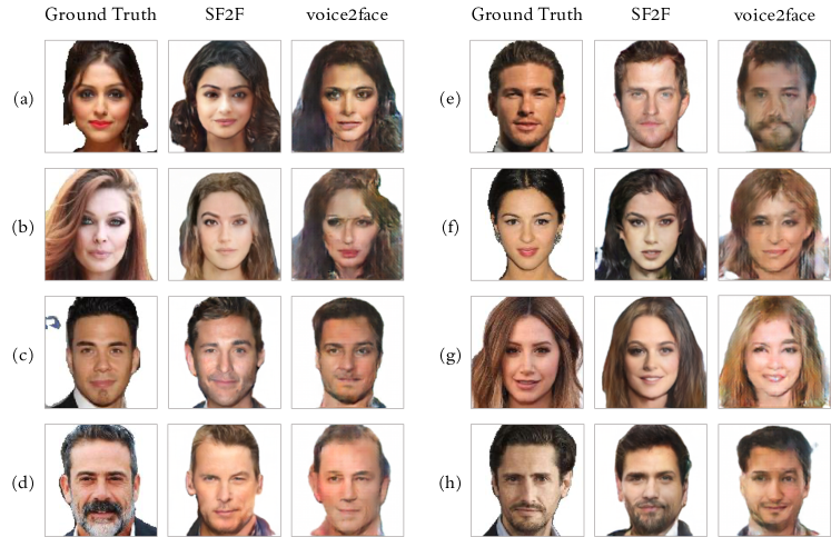
Figure 6: Examples of 128 $\times$ 128 generated images using SF2F and voice2face

Appendix B Data Quality Enhancement

B.1 HQ-VoxCeleb Dataset

As an overview of the HQ-VoxCeleb dataset is presented in the main paper, in this section, we elaborate on the standards and process in our data enhancement scheme. As demonstrated in Fig. 7, the poor quality of training dataset for speech2face is one of the major factors hindering the improvement of speech2face performance. To eliminate the negative impact of the training data itself, we carefully design and build a new high-quality face database on top of VoxCeleb dataset, such that face images associated with the celebrities are all at reasonable quality.

To fulfill the vision of data quality, we set a number of general guidelines over the face images as the underlying measurement on quality, as follows:

• Face angle between human’s facial plane and the photo imaging plane is no larger than 5^∘;

• Lighting condition on the face is generally uniform, without any noticeable shadow and sharp illumination change;

• Expression on the human faces is generally neutral, while minor smile expression is also acceptable;

• Background does not contain irrelevant information in the image, and completely void background in white is preferred.

To fully meet the standards as listed above, we adopt the following methodology to build the enhanced HQ-VoxCeleb dataset for our speech2face model training.

Figure 7: The quality variance of the original manually filtered VGGFace dataset (on the right of the figure) [8] diverts the efforts of face generator model to the normalization of the faces. By filtering and correcting the face database (on the left), the computer vision models are expected to focus more on the construction of mapping between vocal features and physical facial features.

Data Collection. We collect 300 in-the-wild images for each of the 7,363 individuals in VoxCeleb dataset, by crawling images of the celebrities on the Internet. The visual qualities of the retrieved images are highly diverse. The resolution of the images, for example, ranges from 47$\times$59 to 6245$\times$8093 in pixels. Moreover, some of the images cover the full body of the celebrity of interest, while other images only include the face of the target individual. It is, therefore, necessary to apply pre-processing and filtering operations to ensure 1) the variance of the image quality is reasonably small; and 2) all the images are centered at the face of the target individuals.

Machine Filtering. To filter out unqualified images from the massive in-the-wild images, we deploy an automated filtering module, together with a suite of concrete selection rules, to eliminate images at poor quality, before dispatching the images for human filtering. In the filtering module, the algorithm first detects the landmarks from the raw face images. Based on the output landmarks of the faces, the algorithm identifies poorly posed faces, if the landmarks from left/right sides cannot be well aligned. Low-resolution face images, with distance between pupils covers fewer than 30 pixels, are also removed. Finally, a pre-trained CNN classifier [46] is deployed to infer the emotion of the individual in the image, such that faces not recognized as "neutral” emotion are also removed from the dataset.

Image Processing. Given the face images passing the first round machine-based filtering, we apply a two-step image processing, namely face alignment and image segmentation in the second round of filtering. In the first step of face alignment, the images are rotated and cropped to make sure both the pupils of the faces in all these images are always at the same coordinates. In the second step of image segmentation, we apply a pyramid scene parsing network [47] pre-trained on Pascal VOC 2012 dataset [48] to split the target individuals from the background in the images. The background is then refilled with white pixels. Note that the second step is helpful because irrelevant noise in the background may potentially confuse the generation model.

Human Filtering. To guarantee the final quality of the images in HQ-VoxCeleb dataset, human workers are employed to select 3 to 7 images at best qualities for each celebrity. Only celebrities with at least 3 qualified face images are kept in the final dataset.

B.2 Comparison with Existing Datasets

In the main paper, we summarize the statistics of the result dataset after the adoption of the processing steps above. In this section, we compare HQ-VoxCeleb with existing audiovisual datasets [26, 25, 49, 7, 6] in terms of data quality and its impact to model training, in order to justify the contribution of HQ-VoxCeleb. Table 6 shows the attributes of existing audiovisual datasets.

Existing datasets, including VoxCeleb [6, 7] and AVSpeech [49], contain a massive number of pairwise data of human speech and face images. However, the existing datasets are constructed by cropping face images and speech audio from in-the-wild online data, and the face images thus vary hugely in pose, lighting, and emotion, which makes the existing datasets unfit for end-to-end learning of speech-to-face algorithms. To the highest image quality of existing datasets, Wen et al. [5] use the intersection of the filtered VGGFace [26] and VoxCeleb with the common identities. However, as shown in Fig. 7, the filtered VGGFace cannot meet the quality standards defined in section B.1. Moreover, HQ-VoxCeleb has triple as many identities as filtered VGGFace as shown in Table 6. In conclusion, the high quality and reasonable amount of data make HQ-VoxCeleb the most suitable dataset for speech2face tasks.

Table 6: The attributes of HQ-VoxCeleb and existing audiovisual datasets

Dataset	#Identity	#Image	#Speech	Normalized Faces
FVMatching [26]	1,078	118,553	131,815	No
FVCeleb [25]	181	181	239	No
AVSpeech [49]	100,000+	-	-	No
VoxCeleb [7, 6]	7,245	-	1,237,274	No
Filtered VGGFace [8, 5]	1,225	139,572	149,354	No
HQ-VoxCeleb	3,638	8,028	609,700	Yes

Appendix C Additional Experimental Results

C.1 Ablation Study

In this section, we focus on the effectiveness evaluation over the model components, loss functions, and dataset used in our SF2F approach. The ablated models are trained to generate $64\times 64$ images, with all the results are summarized in Table 7. When removing any of the four loss functions in $\{L_{1},L_{G},L_{C},L_{P}\}$, the performance of SF2F drops accordingly. This shows it is necessary to include all these components to ensure the learning procedure of the model is well balanced. 1D-CNN encoder is used in the baseline approach [5], while SF2F employs 1D-Inception encoder instead. We report the performance of SF2F by substituting our encoder with 1D-CNN, referred to as Baseline Encoder in Table 7. This replacement causes a significant drop of the performance on all metrics. Similarly, by adopting the deconvolution-based decoder used in [5, 4] instead of the upsampling-and-convolution-based decoder in SF2F, referred as Baseline Decoder in Table 7, we observe a slight yet consistent performance drop. The impact of data quality is also evaluated, by training the SF2F model with the manually filtered version of VGGFace dataset [8] instead of HQ-VoxCeleb, by including overlap celebrity individuals included in both datasets. Poor data quality obviously leads to a huge performance plunge, which further justifies the importance of training data quality enhancement.

Table 7: Ablation Study on HQ-VoxCeleb dataset

Setting	Similarity		Retrieval				Quality
Ablation	cosine	L1	R@1	R@2	R@5	R@10	VFS
w/o $L_{1}$	0.310	21.74	3.47	7.26	18.36	31.56	16.84
w/o $L_{G}$	0.298	20.97	3.23	8.70	16.73	32.36	18.51
w/o $L_{C}$	0.310	18.13	5.24	8.45	17.30	34.28	19.16
w/o $L_{P}$	0.236	18.22	2.73	5.23	15.39	26.37	18.44
Baseline Encoder	0.309	18.47	5.54	9.26	19.18	34.75	18.89
Baseline Decoder	0.311	18.52	4.32	8.56	19.47	34.25	18.46
LQ. Dataset	0.267	19.94	1.96	4.21	10.67	21.34	16.73
Full Model	0.317	17.91	5.75	9.32	20.36	36.65	19.49

C.2 Performance on Filtered VGGFace

We also compare the performance of SF2F and voice2face [5] on the filtered VGGFace dataset [8], to evaluate how SF2F functions under less controlled conditions. To make a fair comparison, we train both models with filtered VGGFace dataset. Both voice2face and our SF2F are trained to generate images with 64$\times$64 pixels, and evaluated with 1.25 seconds and 5 seconds of human speech clips. As is presented in Table 8, SF2F outperforms voice2face by a large margin on all metrics. By deploying fuser in SF2F, the maximal recall@10 reaches 21.34%, significantly outperforming voice2face.

Table 8: Performance on filtered VGGFace dataset in feature similarity, retrieval recall@K, and VGGFace Score

Setting		Similarity		Retrieval				Quality
Method	Len.	cosine	L1	R@1	R@2	R@5	R@10	VFS
random	-	-	-	1.00	2.00	5.00	10.00	-
voice2face	1.25 sec	0.164	26.45	1.46	3.12	7.25	20.71	12.94 $\pm$ 0.57
SF2F (no fuser)	1.25 sec	0.251	21.23	1.81	4.05	9.77	18.56	16.62 $\pm$ 0.44
voice2face	5 sec	0.165	26.42	1.45	3.17	7.89	15.43	12.72 $\pm$ 0.73
SF2F (no fuser)	5 sec	0.248	21.46	1.77	3.98	9.75	18.36	16.49 $\pm$ 0.83
SF2F	5 sec	0.267	19.94	1.96	4.21	10.67	21.34	16.73 $\pm$ 0.67

Appendix D Model Details

D.1 Voice Encoder

We use a 1D-CNN composed of several 1D Inception modules [35] to process mel-spectrogram. The voice encoder module converts each short input speech segment into a predicted facial feature embedding. The architecture of the 1D Inception module and the voice encoder is summarized in Table 9. The Inception module models various ranges of short-term mel-spectrogram dependency, and enables more accurate information flow from voice domain to image domain, compared to plain single-kernel-size CNN used in [5].

Table 9: The detailed structure of the 1D Inception module and voice encoder. In the descriptions, Conv $x$/$y$ denotes 1D convolution with kernel size of $x$ and stride length of $y$.

1D Inception Module
Component	Activation	Dimension
Input	-	$d_{i}\times t_{i}$
Conv 2/2	BN + ReLU	$d\times t_{o}$
Conv 3/2	BN + ReLU	$d\times t_{o}$
Conv 5/2	BN + ReLU	$d\times t_{o}$
Conv 7/2	BN + ReLU	$d\times t_{o}$
Concat.	-	$4d\times t_{o}$

Voice Encoder
Layer	Dimension
Input	$40\times t_{0}$
Inception 1	$256\times t_{1}$
Inception 2	$384\times t_{2}$
Inception 3	$576\times t_{3}$
Inception 4	$864\times t_{4}$
Inception 5	$512\times t_{5}$
Time AvePool	$512\times 1$

D.2 Face Decoder

D.2.1 Single-resolution Decoder

The face decoder reconstructs the target individual’s face image based on the embeddings extracted from the individual’s speech segments. The architectures of the upsampling block (UpBlock) and the face decoder are summarized in Table 10. We show the structure of the face decoder generating 64$\times$64 images, and the face decoder generating 128$\times$128 images can be built by adding UpBlock 7 after UpBlock 6. Our empirical evaluations prove that our decoder based on upsampling and convolution renders better performance in all the metrics compared to the deconvolution-based decoder employed in existing studies [4] and [5].

Table 10: The detailed structure of the upsampling block and face decoder. In the descriptions, Conv $x_{/y,z}$ denotes 2D convolution with kernel size of $x$, stride length of $y$, and padding size of $z$.

Upsampling Block
Component	Dimension
Input	$d_{i}\times w_{i}\times w_{i}$
Upsampling	$d_{i}\times 2w_{i}\times 2w_{i}$
Conv $3_{/2,1}$	$d\times 2w_{i}\times 2w_{i}$
ReLU	$d\times 2w_{i}\times 2w_{i}$
Batch Norm	$d\times 2w_{i}\times 2w_{i}$

Face Decoder
Layer	Dimension
Input	$512\times 1\times 1$
UpBlock 1	$1024\times 2\times 2$
UpBlock 2	$512\times 4\times 4$
UpBlock 3	$256\times 8\times 8$
UpBlock 4	$128\times 16\times 16$
UpBlock 5	$64\times 32\times 32$
UpBlock 6	$32\times 64\times 64$
Conv $1_{/1,0}$	$3\times 64\times 64$

D.2.2 Multi-resolution Decoder

Inspired by [50], the multi-resolution decoder is optimized to generate images at both low resolution and high resolution, which is shown in Fig. 8. With the multi-resolution approach, the decoder learns to model the multiple target domain distributions of different scales, which helps to overcome the difficulty of generating high-resolution images.

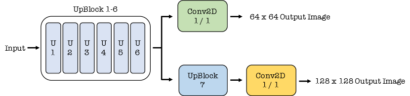
Figure 8: Structure of the multi-resolution face decoder

D.3 Discriminators

The network structure of image discriminator $D_{real}$ and identity classifier $D_{id}$ is described in Table 11. Both networks are convolutional neural networks, followed by fully connected networks. In Table 11, we demonstrate the structure of discriminators for 64 $\times$ 64 images, and the discriminator of 128 $\times$ 128 images can be simply implemented by adding another convolution layer before average pooling layer.

Table 11: The structure of the discriminators for 64 $\times$ 64 images. In this table, Conv $x_{/y,z}$ denotes 2D convolution with kernel size of $x$, stride length of $y$, and padding size of $z$. $d_{o}=2$ for binary image discriminator, and $d_{o}=N_{id}$ for identity classifier.

Discriminator Network
Component	Activation	Dimension
Input	-	$3\times 64\times 64$
Conv $4_{/2,1}$	BN + ReLU	$64\times 32\times 32$
Conv $4_{/2,1}$	BN + ReLU	$128\times 16\times 16$
Conv $4_{/2,1}$	BN + ReLU	$256\times 8\times 8$
Avg. Pooling	-	$256\times 1\times 1$
Linear	ReLU	$1024$
Linear	Softmax	$d_{o}$

D.4 Complexity Analysis of SF2F model

Shown in Table 12 is the time and space complexity of each component of SF2F model, where $t$ stands for the length of the input audio and $w$ stands for the dimension of the output face image. The time complexity of convolution and attention is $\Omega(1)$ regardless of the input length. The space complexity of 1D convolution is $O(t)$ and the space complexity of self attention is $O(t^{2})$.

Table 12: Complexity analysis

Component	Time Complexity	Space Complexity
Voice Encoder	$\Omega(1)$	$O(t)$
Embedding Fuser	$\Omega(1)$	$O(t^{2})$
Face Decoder	$\Omega(1)$	$O(w^{2})$

Appendix E Implementation Details

E.1 Training

We train all our SF2F models on 1 NVIDIA V100 GPU with 32 GB memory; SF2F is implemented with PyTorch [51]. The encoder-decoder training takes 120,000 iterations, and the fuser training takes 360 iterations. The training of 64 $\times$ 64 models takes about 18 hours, and the training of 128 $\times$ 128 models takes about 32 hours. The model is trained only once in each experiment.

E.2 Evaluation

Evaluation is conducted on the same GPU machine. The details of the implementation are provided in this part of the section.

Ground Truth Embedding Matrix.

As mentioned in the main paper, the ground truth embedding matrix $U=\{u_{1},u_{2},\ldots,u_{N}\}$ extracted by FaceNet [39] is used for similarity metric and retrieval metric. Given that one identity is often associated with multiple, i.e., $K$, face images in both datasets, for an identity of index $n$, the ground truth embedding is computed by ${u}_{n}=\sum^{K}_{j=1}u_{nj}/K$. The embedding $u_{n}$ is normalized as $u_{n}=\frac{u_{n}}{\max(\lVert u_{n}\rVert_{2},\epsilon)}$, because the embeddings extracted by FaceNet are also L2 normalized. Building embedding matrix with all the image data helps remove variance in data. This makes the evaluation results fair and stable.

Evaluation Runs.

In each experiment, we randomly crop 10 pieces of audio with desired length for each identity in the evaluation dataset. With the data above, each experiment is evaluated ten times, the mean of each metric is calculated based on the outcomes of all these ten evaluation runs. We additionally report the variance of VGGFace Score.

E.3 Hyperparameter

The hyperparameters for SF2F’s model training are listed in Table 13. The detailed configuration of SF2F’s network is available in Section D as well as the main paper.

Table 13: Hyperparameters of SF2F

Hyperparameter	Value
Optimizer	Adam [38]
Optimizer $\beta_{1}$	0.9
Optimizer $\beta_{2}$	0.98
Learning Rate	5e-4
Batch Size	256
$\lambda_{1}$	10
$\lambda_{2}$	1
$\lambda_{3}$	0.05
$\lambda_{4}$	100
Fuser Dimension	512

Hyperparameters are carefully tuned. As the training is time-consuming and the hyperparameter space is large, it is difficult to apply grid search directly. We adopt other methods for parameter tuning instead.

We first train a SF2F model with $\lambda_{1},\lambda_{2},\lambda_{3}=1$ and $\lambda_{4}=0$, we adjust the parameters $\lambda_{1}$ and $\lambda_{3}$ and find that increasing the Image Reconstruction Loss weight $\lambda_{1}$ and decreasing the Auxiliary Classifier Loss weight $\lambda_{3}$ both improve the model performance. We adjust $\lambda_{1}$ and $\lambda_{3}$ gradually and find out the model achieves the best performance when $\lambda_{1}=10$ and $\lambda_{3}=0.05$ . Afterward, we apply Perceptual Loss to our model training with initial weight $\lambda_{4}=1$. We find increasing $\lambda_{4}$ improves SF2F’s performance, which is because the original scale of Perceptual Loss is much smaller than the scale of the other three losses. We gradually increase $\lambda_{4}$ until we observe SF2F achieving the best performance when $\lambda_{4}=100$. Therefore, $\lambda_{1},\lambda_{2},\lambda_{3},\lambda_{4}$ are set at 10, 1, 0.05 and 100, respectively.

Afterwards, we apply a grid search over learning rate and batch size. We test with different values, which are listed in Table 14 with optimal values singled out in the last column.

Table 14: The values considered for grid search

Hyperparamter	Values Considered	Optimal Value
Learning Rate	1e-4, 2e-4, 5e-4, 1e-3	5e-4
Batch Size	64, 128, 256, 512	256

The hyperparameters above are determined by tuning a $64\times 64$ SF2F model with HQ-VoxCeleb dataset, and we find this hyperparameter configuration works well with $128\times 128$ SF2F model. With this hyperparameter configuration, SF2F outperforms voice2face on filtered VGGFace dataset. Consequently, we opt to skip further hyperparameter tuning on filtered VGGFace. The total cost of hyperparameter tuning is around 558 GPU hours on V100.

References

- [1] Yunjey Choi, Min-Je Choi, Munyoung Kim, Jung-Woo Ha, Sunghun Kim, and Jaegul Choo. Stargan: Unified generative adversarial networks for multi-domain image-to-image translation. In 2018 IEEE Conference on Computer Vision and Pattern Recognition, CVPR 2018, Salt Lake City, UT, USA, June 18-22, 2018, pages 8789–8797, 2018.
- [2] Yunjey Choi, Youngjung Uh, Jaejun Yoo, and Jung-Woo Ha. Stargan v2: Diverse image synthesis for multiple domains. CoRR, abs/1912.01865, 2019.
- [3] Tero Karras, Samuli Laine, and Timo Aila. A style-based generator architecture for generative adversarial networks. In IEEE Conference on Computer Vision and Pattern Recognition, CVPR 2019, Long Beach, CA, USA, June 16-20, 2019, pages 4401–4410. Computer Vision Foundation / IEEE, 2019.
- [4] Tae-Hyun Oh, Tali Dekel, Changil Kim, Inbar Mosseri, William T. Freeman, Michael Rubinstein, and Wojciech Matusik. Speech2face: Learning the face behind a voice. In The IEEE Conference on Computer Vision and Pattern Recognition (CVPR), June 2019.
- [5] Yandong Wen, Bhiksha Raj, and Rita Singh. Face reconstruction from voice using generative adversarial networks. In Advances in Neural Information Processing Systems, pages 5266–5275, 2019.
- [6] Joon Son Chung, Arsha Nagrani, and Andrew Zisserman. Voxceleb2: Deep speaker recognition. In Interspeech, pages 1086–1090, 2018.
- [7] Arsha Nagrani, Joon Son Chung, and Andrew Zisserman. Voxceleb: A large-scale speaker identification dataset. In Interspeech, pages 2616–2620, 2017.
- [8] Omkar M Parkhi, Andrea Vedaldi, and Andrew Zisserman. Deep face recognition. 2015.
- [9] Li Wan, Quan Wang, Alan Papir, and Ignacio Lopez-Moreno. Generalized end-to-end loss for speaker verification. In ICASSP, pages 4879–4883, 2018.
- [10] Aaron van den Oord, Nal Kalchbrenner, and Koray Kavukcuoglu. Pixel recurrent neural networks. arXiv preprint arXiv:1601.06759, 2016.
- [11] Diederik P Kingma and Max Welling. Auto-encoding variational bayes. arXiv preprint arXiv:1312.6114, 2013.
- [12] Yunchen Pu, Zhe Gan, Ricardo Henao, Xin Yuan, Chunyuan Li, Andrew Stevens, and Lawrence Carin. Variational autoencoder for deep learning of images, labels and captions. In D. D. Lee, M. Sugiyama, U. V. Luxburg, I. Guyon, and R. Garnett, editors, Advances in Neural Information Processing Systems 29, pages 2352–2360. Curran Associates, Inc., 2016.
- [13] Ian Goodfellow, Jean Pouget-Abadie, Mehdi Mirza, Bing Xu, David Warde-Farley, Sherjil Ozair, Aaron Courville, and Yoshua Bengio. Generative adversarial nets. In Z. Ghahramani, M. Welling, C. Cortes, N. D. Lawrence, and K. Q. Weinberger, editors, Advances in Neural Information Processing Systems 27, pages 2672–2680. Curran Associates, Inc., 2014.
- [14] Alec Radford, Luke Metz, and Soumith Chintala. Unsupervised representation learning with deep convolutional generative adversarial networks. arXiv preprint arXiv:1511.06434, 2015.
- [15] Sarah Taylor, Taehwan Kim, Yisong Yue, Moshe Mahler, James Krahe, Anastasio Garcia Rodriguez, Jessica Hodgins, and Iain Matthews. A deep learning approach for generalized speech animation. ACM Transactions on Graphics (TOG), 36(4):1–11, 2017.
- [16] Tero Karras, Timo Aila, Samuli Laine, Antti Herva, and Jaakko Lehtinen. Audio-driven facial animation by joint end-to-end learning of pose and emotion. ACM Transactions on Graphics (TOG), 36(4):1–12, 2017.
- [17] Supasorn Suwajanakorn, Steven M Seitz, and Ira Kemelmacher-Shlizerman. Synthesizing obama: learning lip sync from audio. ACM Transactions on Graphics (TOG), 36(4):1–13, 2017.
- [18] Najmeh Sadoughi and Carlos Busso. Speech-driven expressive talking lips with conditional sequential generative adversarial networks. IEEE Transactions on Affective Computing, 2019.
- [19] Olivia Wiles, A Sophia Koepke, and Andrew Zisserman. X2face: A network for controlling face generation using images, audio, and pose codes. In Proceedings of the European Conference on Computer Vision (ECCV), pages 670–686, 2018.
- [20] Xavier Giro, Amanda Duarte, Francisco Roldan, Miquel Tubau, Janna Escur, Santiago Pascual, Amaia Salvador, Eva Mohedano, Kevin McGuinness, Jordi Torres, et al. Wav2pix: Speech-conditioned face generation using generative adversarial networks. 2019.
- [21] Suwon Shon, Tae-Hyun Oh, and James Glass. Noise-tolerant audio-visual online person verification using an attention-based neural network fusion. In ICASSP 2019-2019 IEEE International Conference on Acoustics, Speech and Signal Processing (ICASSP), pages 3995–3999. IEEE, 2019.
- [22] Arsha Nagrani, Samuel Albanie, and Andrew Zisserman. Learnable pins: Cross-modal embeddings for person identity. In Proceedings of the European Conference on Computer Vision (ECCV), pages 71–88, 2018.
- [23] Arsha Nagrani, Samuel Albanie, and Andrew Zisserman. Seeing voices and hearing faces: Cross-modal biometric matching. In Proceedings of the IEEE conference on computer vision and pattern recognition, pages 8427–8436, 2018.
- [24] Yandong Wen, Mahmoud Al Ismail, Weiyang Liu, Bhiksha Raj, and Rita Singh. Disjoint mapping network for cross-modal matching of voices and faces. arXiv preprint arXiv:1807.04836, 2018.
- [25] Changil Kim, Hijung Valentina Shin, Tae-Hyun Oh, Alexandre Kaspar, Mohamed Elgharib, and Wojciech Matusik. On learning associations of faces and voices. In Asian Conference on Computer Vision, pages 276–292. Springer, 2018.
- [26] Shota Horiguchi, Naoyuki Kanda, and Kenji Nagamatsu. Face-voice matching using cross-modal embeddings. In Proceedings of the 26th ACM international conference on Multimedia, pages 1011–1019, 2018.
- [27] Joon Son Chung, Andrew Senior, Oriol Vinyals, and Andrew Zisserman. Lip reading sentences in the wild. In 2017 IEEE Conference on Computer Vision and Pattern Recognition (CVPR), pages 3444–3453. IEEE, 2017.
- [28] Jiquan Ngiam, Aditya Khosla, Mingyu Kim, Juhan Nam, Honglak Lee, and Andrew Y Ng. Multimodal deep learning. 2011.
- [29] Ken Hoover, Sourish Chaudhuri, Caroline Pantofaru, Malcolm Slaney, and Ian Sturdy. Putting a face to the voice: Fusing audio and visual signals across a video to determine speakers. arXiv preprint arXiv:1706.00079, 2017.
- [30] Israel D Gebru, Sileye Ba, Georgios Evangelidis, and Radu Horaud. Tracking the active speaker based on a joint audio-visual observation model. In Proceedings of the IEEE International Conference on Computer Vision Workshops, pages 15–21, 2015.
- [31] Samuel Albanie, Arsha Nagrani, Andrea Vedaldi, and Andrew Zisserman. Emotion recognition in speech using cross-modal transfer in the wild. In Proceedings of the 26th ACM international conference on Multimedia, pages 292–301, 2018.
- [32] Galen Andrew, Raman Arora, Jeff Bilmes, and Karen Livescu. Deep canonical correlation analysis. In International conference on machine learning, pages 1247–1255, 2013.
- [33] Forrester Cole, David Belanger, Dilip Krishnan, Aaron Sarna, Inbar Mosseri, and William T. Freeman. Synthesizing normalized faces from facial identity features. In The IEEE Conference on Computer Vision and Pattern Recognition (CVPR), July 2017.
- [34] Meinard Müller. Fundamentals of music processing: Audio, analysis, algorithms, applications. Springer, 2015.
- [35] Christian Szegedy, Wei Liu, Yangqing Jia, Pierre Sermanet, Scott Reed, Dragomir Anguelov, Dumitru Erhan, Vincent Vanhoucke, and Andrew Rabinovich. Going deeper with convolutions. In Proceedings of the IEEE conference on computer vision and pattern recognition, pages 1–9, 2015.
- [36] Sergey Ioffe and Christian Szegedy. Batch normalization: Accelerating deep network training by reducing internal covariate shift. arXiv preprint arXiv:1502.03167, 2015.
- [37] Justin Johnson, Alexandre Alahi, and Li Fei-Fei. Perceptual losses for real-time style transfer and super-resolution. In European conference on computer vision, pages 694–711. Springer, 2016.
- [38] Diederik P. Kingma and Jimmy Ba. Adam: A method for stochastic optimization. In ICLR, 2015.
- [39] Florian Schroff, Dmitry Kalenichenko, and James Philbin. Facenet: A unified embedding for face recognition and clustering. In Proceedings of the IEEE conference on computer vision and pattern recognition, pages 815–823, 2015.
- [40] Tim Salimans, Ian Goodfellow, Wojciech Zaremba, Vicki Cheung, Alec Radford, and Xi Chen. Improved techniques for training gans. In Advances in neural information processing systems, pages 2234–2242, 2016.
- [41] Justin Johnson, Agrim Gupta, and Li Fei-Fei. Image generation from scene graphs. In Proceedings of the IEEE conference on computer vision and pattern recognition, pages 1219–1228, 2018.
- [42] Tao Xu, Pengchuan Zhang, Qiuyuan Huang, Han Zhang, Zhe Gan, Xiaolei Huang, and Xiaodong He. Attngan: Fine-grained text to image generation with attentional generative adversarial networks. In Proceedings of the IEEE conference on computer vision and pattern recognition, pages 1316–1324, 2018.
- [43] LI Yikang, Tao Ma, Yeqi Bai, Nan Duan, Sining Wei, and Xiaogang Wang. Pastegan: A semi-parametric method to generate image from scene graph. In Advances in Neural Information Processing Systems, pages 3950–3960, 2019.
- [44] Han Zhang, Tao Xu, Hongsheng Li, Shaoting Zhang, Xiaogang Wang, Xiaolei Huang, and Dimitris N Metaxas. Stackgan: Text to photo-realistic image synthesis with stacked generative adversarial networks. In Proceedings of the IEEE international conference on computer vision, pages 5907–5915, 2017.
- [45] Yandong Wen, Bhiksha Raj, and Rita Singh. Implementation of reconstructing faces from voices paper. https://github.com/cmu-mlsp/reconstructing_faces_from_voices. Accessed: 2020-5-29.
- [46] Octavio Arriaga, Matias Valdenegro-Toro, and Paul Plöger. Real-time convolutional neural networks for emotion and gender classification. arXiv preprint arXiv:1710.07557, 2017.
- [47] Hengshuang Zhao, Jianping Shi, Xiaojuan Qi, Xiaogang Wang, and Jiaya Jia. Pyramid scene parsing network. In Proceedings of the IEEE conference on computer vision and pattern recognition, pages 2881–2890, 2017.
- [48] M. Everingham, L. Van Gool, C. K. I. Williams, J. Winn, and A. Zisserman. The PASCAL Visual Object Classes Challenge 2012 (VOC2012) Results. http://www.pascal-network.org/challenges/VOC/voc2012/workshop/index.html.
- [49] Ariel Ephrat, Inbar Mosseri, Oran Lang, Tali Dekel, Kevin Wilson, Avinatan Hassidim, William T Freeman, and Michael Rubinstein. Looking to listen at the cocktail party: A speaker-independent audio-visual model for speech separation. arXiv preprint arXiv:1804.03619, 2018.
- [50] Han Zhang, Tao Xu, Hongsheng Li, Shaoting Zhang, Xiaogang Wang, Xiaolei Huang, and Dimitris N Metaxas. Stackgan++: Realistic image synthesis with stacked generative adversarial networks. IEEE transactions on pattern analysis and machine intelligence, 41(8):1947–1962, 2018.
- [51] Adam Paszke, Sam Gross, Francisco Massa, Adam Lerer, James Bradbury, Gregory Chanan, Trevor Killeen, Zeming Lin, Natalia Gimelshein, Luca Antiga, et al. Pytorch: An imperative style, high-performance deep learning library. In Advances in Neural Information Processing Systems, pages 8024–8035, 2019.