Optimal quantum phase estimation in an atomic gyroscope based on Bose-Hubbard model

Abstract

We investigate the optimal quantum state for an atomic gyroscope based on a three-site Bose-Hubbard model. In previous studies, various states such as the uncorrelated state, the BAT state and the NOON state are employed as the probe states to estimate the phase uncertainty. In this article, we present a Hermitian operator $\mathcal{H}$ and an equivalent unitary parametrization transformation to calculate the quantum Fisher information for any initial states. Exploiting this equivalent unitary parametrization transformation, we can seek the optimal state which gives the maximal quantum Fisher information on both lossless and lossy conditions. As a result, we find that the entangled even squeezed state (EESS) can significantly enhance the precision for moderate loss rates.

I Introduction

In recent decades, the technology of quantum physics plays an important role in precision measurements and the accuracy has been improved significantly in comparison with classical systems. The advantages of quantum technology are reflected in various fields such as the biological sensing Taylor and Bowen (2016); Taylor et al. (2013); Nasr et al. (2009); Morris et al. (2015), the measurements of physical constants Fixler et al. (2007); Hu et al. (2013); Lamporesi et al. (2008), and the gravitational wave detection Demkowicz-Dobrzański et al. (2013); Purdy et al. (2013); Punturo et al. (2010); Braginsky and Vyatchanin (2004); Adhikari (2014); McGuirk et al. (2002). In quantum metrology, the optical interferometer such as the Mach-Zehnder (MZ) interferometer is frequently used to estimate the relative phase of two modes, and the precision obtained by using classic states can reach the standard quantum limit (SQL), i.e., $1/\sqrt{N}$ , where $N$ is the total mean number of photons of two modes. In 1981, a typical scheme proposed by Caves Caves (1981) is to take a coherent state $\left|\alpha\right\rangle$ and a squeezed vacuum state $\left|\xi\right\rangle$ as the input states of the Mach-Zehnder interferometer, which can beat the SQL. On the other hand, the unique characteristics of quantum states such as entanglement provide us with a way to reach the Heisenberg limit, i.e., $1/N$, and the NOON state Dorner et al. (2009); Lee et al. (2002); Cooper et al. (2010); Tsarev et al. (2018) is widely studied since its quantum property of maximal entanglement and superior performance in metrology. Based on the result of the NOON state, the entangled coherent state (ECS) Joo et al. (2011, 2012); Zhang et al. (2013); Liu et al. (2016) which is viewed as a similar probe state, gives a remarkable precision enhancement on both lossless and lossy conditions than the NOON state.

Similar researches for phase estimation can be applied to fiber-optic gyroscopes Arditty and Lefèvre (1981) and atomic gyroscopes, which are designed to measure the phase caused by rotation and broadly used for navigation systems. Atomic gyroscopes have received considerable attention for their excellent performance in enhancing sensitivity of rotation, and atomic Sagnac interferometers such as light-pulse atomic interferometers Gustavson et al. (1997); Kasevich and Chu (1992); Gustavson et al. (2000), and guided matter-wave interferometers Wu et al. (2007); Alzar et al. (2012); Stevenson et al. (2015); Rico-Gutierrez et al. (2015) are widely studied. Another novel type of gyroscope is based on Bose-Hubbard model and it is composed of a collection of ultracold atoms trapped in an optical lattice loop of several sites Cooper et al. (2009, 2010). In Ref. Cooper et al. (2010), Cooper et al. investigated three different input states and found that the NOON state produces the best precision with scaling $1/N$ under lossless conditions. However, considering the presence of particle loss in practical systems, the BAT state is a better choice because of its robustness in high loss regime. In the above studies, quantum Fisher information (QFI) Helstrom (1976); Braunstein and Caves (1994); Holevo (1982); Braunstein et al. (1996); Liu et al. (2019) is an important concept in quantum metrology, which gives the lower limit of the variance of parameter $\theta$ due to the quantum Cramér-Rao bound, i.e.,

$$\Delta\theta\geq\frac{1}{\sqrt{\mu F_{Q}}},$$ (1)

where $\mu$ is the number of independent repeats of the experiment and $F_{Q}$ is the QFI. Hence, the core task in many studies is trying every means to obtain larger QFI. For a general measurement scheme, quantum states passing through an atomic gyroscope or optical devices will cause a phase $\theta$, and such a variation can be regarded as a unitary parametrization processes $U(\theta)$. For a pure initial state $\left|\psi\right\rangle_{\rm in}$, the QFI with respect to the parameter $\theta$ is defined as Pang and Brun (2014); Liu et al. (2015); Jing et al. (2015)

$$F_{Q}=4\left(\left\langle\mathcal{H}^{2}\right\rangle-\left\langle\mathcal{H}\right\rangle^{2}\right),$$ (2)

where

$$\mathcal{H}\equiv i\left(\partial_{\theta}U^{\dagger}\right)U$$ (3)

is a Hermitian operator and the QFI is determined by the variance of $\mathcal{H}$. Thus the dynamical property of a definite unitary parametrization process is characterized by a fixed $\mathcal{H}$, and the optimal probe state could be gotten by comparing various input states.

In this article, we follow the work of the Ref. Cooper et al. (2010), and propose an equivalent unitary parametrization processes $U_{\rm eq}$ to calculate the highest precision we can reach with the atomic gyroscope introduced above. Although three input states, i.e., the uncorrelated state, the BAT state and the NOON state have been discussed before, there are still superior states can be chosen to boost the precision. We also investigate the effects of particle loss in the atomic gyroscope. In principle, the maximally entangled states such as the NOON state are vulnerable, and the phase information will be rapidly lost when decoherence occurs Cooper et al. (2010); Joo et al. (2011); Tsarev et al. (2018); Huver et al. (2008). Therefore, it is important to find a state that can reach the Heisenberg limit and meanwhile has good robustness against decoherence. Apart from the ECS involved in Ref. Joo et al. (2011), the squeezed entangled state (SES) Knott et al. (2016); Lee et al. (2016); Rubio and Dunningham (2019) which can be regarded as the superposition of NOON states with different even particle numbers shows great potential. The comparison between the ECS and the SES is similar to the relationship between the uncorrelated state and the BAT state discussed in Ref. Cooper et al. (2010), which shows the superposition of even number states produces better precision and robustness than the superposition of the general number states. Furthermore, Refs. Lee et al. (2016); Knott et al. (2016) indicate that the Mandel $\mathcal{Q}$-parameter of the single-mode in a path-symmetric state determines the upper limit of precision. Inspired by these work , we seek for a state can give larger Mandel-$\mathcal{Q}$ parameter, and this leads us to propose "entangled even squeezed state" (EESS). The numerical simulation show that the EESS can give a significant precision enhancement in the small-particle-number regime, and this advantage is maintained until particle loss is larger than $50\%$.

This article is organized as follow. In Section II, we give a Hermitian operator and general expression to calculate the QFI of atomic gyroscope. In In Section III, we discuss the influence of different initial state on the precision in lossless case. In Section IV, we consider the effects of particle loss on the atomic gyroscope.

II GENERAL EXPRESSION OF QFI

First of all, it is necessary to review the procedure of phase measurement in Ref. Cooper et al. (2010). The atomic gyroscope is composed of $N$ ultracold atoms of mass $m$ trapped in an optical lattice loop of three sites where the circumference of the loop is $L$ Hallwood et al. (2007); Cooper et al. (2009); Dunningham et al. (2012), and a schematic diagram is shown in Fig. 1. This scheme can be described by Bose-Hubbard Hamiltonian

$$\frac{H}{\hbar}=\sum_{i=0}^{2}\epsilon_{i}a_{i}^{\dagger}a_{i}-\sum_{i=0}^{2}J_{i}\left(a_{i}^{\dagger}a_{i+1}+a_{i+1}^{\dagger}a_{i}\right)+\sum_{i=0}^{2}V_{i}a_{i}^{\dagger 2}a_{i}^{2},$$ (4)

where $a_{i}^{\dagger}$ and $a_{i}$ are creation and annihilation operators in site $i$. The first term accounts for energy offset, and it can be ignored by taking a fixed zero-energy for each site, and we set $\epsilon_{i}=0$. The second term is the coupling between site $i$ and site $i+1$ , and the last term represents the interaction between atoms on each site. Moreover, the strengths of coupling energy and interaction energy are described by the parameters $J_{i}$ and $V_{i}$ respectively, and the latter can be ignored compared with the former when the potential barrier between two sites is reduced, i.e., $V_{i}\approx 0$. This system is described in detail in Ref. Cooper et al. (2009). Therefore, the unitary transformation $U=e^{-iHt/\hbar}$ only depends on the coupling energy in the high coupling regime. It is convenient to diagonalize the Hamiltonian by using the quasi-momentum basis, or flow basis, Hallwood et al. (2007); Dunningham et al. (2012); Hallwood et al. (2006), i.e.,

$$\begin{pmatrix}\alpha_{-\!\!1}\\ \alpha_{\,0}\\ \alpha_{\,1}\end{pmatrix}=\frac{1}{\sqrt{3}}\begin{pmatrix}1&e^{-i2\pi/3}&e^{i2\pi/3}\\ 1&1&1\\ 1&e^{i2\pi/3}&e^{-i2\pi/3}\end{pmatrix}\begin{pmatrix}a_{0}\\ a_{1}\\ a_{2}\end{pmatrix}$$ (5)

and the Hamiltonian in high coupling regime is given by

$$\frac{H}{\hbar}=-2J\sum_{j=-1}^{1}\cos\left(2\pi j/3\right)\alpha_{j}^{\dagger}\alpha_{j}.$$ (6)

In this way, the three-port beam splitter (tritter) described in Ref. Cooper et al. (2009) is able to be realized. Specifically, the unitary transformation of the tritter is expressed as

$$U_{2} =e^{i\frac{2\pi}{9}\left(a_{0}^{\dagger}a_{1}+a_{1}^{\dagger}a_{2}+a_{2}^{\dagger}a_{0}+h.c.\right)}$$

$$=e^{i\frac{2\pi}{9}\left(2\alpha_{0}^{\dagger}\alpha_{0}-\alpha_{1}^{\dagger}\alpha_{1}-\alpha_{-1}^{\dagger}\alpha_{-1}\right)}$$ (7)

Figure 1: Schematic diagram of the phase estimation in the atomic gyroscope. A quantum state is prepared as an input state of the atomic gyroscope which is a ring configuration of three sites. Then the mechanical rotation of the atomic gyroscope causes a phase $\theta$, and after performing several operations the phase $\theta$ is able to read out.

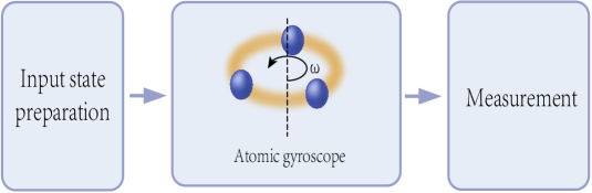
The inverse tritter operation is realized by changing the phase from $2\pi/9$ to $4\pi/9$. The procedure of phase estimation can be briefly summarized as follows: (i) Prepare an initial state. (ii) Perform a tritter operation. (iii) Apply a $2\pi/3$ phase to site two with the unitary transformation $U_{3}=\exp(i2\pi a^{\dagger}_{2}a_{2}/3)$. (iv) Rotate the system with velocity $\omega$. (v) Apply a $-2\pi/3$ phase to site two with the unitary transformation $U_{5}=\exp(-i2\pi a^{\dagger}_{2}a_{2}/3)$. (vi) Perform an inverse tritter operation. (vii) Read out the phase $\theta$ caused by the rotation. The Hamiltonian used in step (iv) is Cooper et al. (2010, 2009)

$$\frac{H_{r}}{\hbar}=-2J\sum_{j=-1}^{1}\cos\left(\theta/3-2\pi j/3\right)\alpha_{j}^{\dagger}\alpha_{j}.$$ (8)

The purpose of step (ii) and step (iii) is to realize the transformation from the particle number states of each site to the flow states, i.e., $\left|l,m,n\right\rangle_{a_{0},a_{1},a_{2}}\Rightarrow$ $\left|l,m,n\right\rangle_{\alpha_{-1},\alpha_{0},\alpha_{1}}$. The term on the left side represents the number of atoms in each site, and the term on the right side represents the number of atoms in the $\alpha_{-1}$,$\alpha_{0}$ and $\alpha_{1}$ flow states, respectively. Similarly, step (v) and step (vi) are the inverse operations of step (ii) and step (iii). One can immediately see that the Hamiltonian in Eq. (8) is diagonalized and can act on the flow states directly. More details of this procedure are described in Ref. Cooper et al. (2010).

To obtain the velocity of rotation more accurately, we need to reduce the variance of $\theta$ since $\Delta\omega=\Delta\theta\cdot\left(h/L^{2}m\right)$. It is worthy to note that the QFI for various initial states only depends on step (i) to (iv), hence the ultimate precision of the atomic gyroscope is able to be calculated by a general Hermitian operator $\mathcal{H}$, which can be expressed as

$$\begin{split}\mathcal{H}&=U_{2}^{\dagger}U_{3}^{\dagger}\mathcal{H}_{4}U_{3}U_{2}\\ &=\frac{-2Jt_{\omega}}{3}\left[\sin\left(\frac{\theta+2\pi}{3}\right)n_{0}+\sin\left(\frac{\theta-2\pi}{3}\right)n_{1}+\sin\left(\frac{\theta}{3}\right)n_{2}\right],\end{split}$$ (9)

where $\mathcal{H}_{4}=i\left(\partial_{\theta}U_{4}^{\dagger}\right)U_{4}=-\partial_{\theta}H_{r}t_{\omega}/\hbar$ according to Eq. (3) and $U_{4}=e^{-iH_{r}t_{\omega}/\hbar}$ is the unitary transformation of rotation, and $t_{\omega}$ is the time the gyroscope takes to rotate. The detailed derivation of $\mathcal{H}$ is presented in Appendix A. Utilizing Eqs. (2) and (9), a general expression of QFI for the atomic gyroscope is obtained, which is helpful to find the optimal state corresponds to this scheme.

In addition, the overall process of phase estimation can be simplified as an equivalent unitary parametrization transformation with Eqs. (3) and (9),

$$\begin{split}U_{\rm eq}&=\exp\left(i\phi_{\,0}n\right)\exp\left(i\phi_{\,1}n_{1}\right)\exp\left(i\phi_{\,2}n_{2}\right)\\ &=\exp\left(i\phi_{\,0}n\right)\exp\left(i\phi_{+}\left(n_{1}+n_{2}\right)/2\right)\exp\left(i\phi_{-}\left(n_{1}-n_{2}\right)/2\right),\end{split}$$ (10)

where $n_{i}=a_{i}^{\dagger}a_{i}$, $n=n_{0}+n_{1}+n_{2}$, and $\phi_{\pm}=\left(\phi_{\,1}\pm\phi_{\,2}\right)$, $\phi_{\,0}=2Jt_{\omega}\cos\left(\theta/3+2\pi/3\right)$, $\phi_{\,1}=2\sqrt{3}Jt_{\omega}\sin\left(\theta/3\right)$, and $\phi_{\,2}=2\sqrt{3}Jt_{\omega}\sin\left(\theta/3+\pi/3\right)$. Actually, it is a hard work to obtain the unitary transformation of this system via multiplying that of each step, however, the approach we used here only needs the calculation of Eq. (9) to get an equivalent unitary parametrization transformation Eq. (10). Note that if the input state is a path-symmetric pure state Jarzyna and Demkowicz-Dobrzański (2012); Knott et al. (2016), a QFI formula for relative phase $\phi_{-}$ will be given by

$$F_{Q}(\phi_{-})=\Delta^{2}\left(n_{1}-n_{2}\right),$$ (11)

and $\Delta\theta$ can be got via the error propagation formula

$$\Delta\theta=\sqrt{3}\Delta\phi_{-}/2Jt_{\omega}\cos\left(\theta/3-\pi/3\right).$$ (12)

III OPTIMAL INPUT STATE

In this section, we investigate the variance of Hermitian operator $\mathcal{H}$ with various input states under the condition of no particle loss. To compare different resources equivalently, we take into account the same average particle number $\bar{n}=N$ for each state.

III.1 Particle number state

First of all, we consider the particle number state which is very common as an input state in quantum metrology. Eq. (9) shows that the Hermitian operator $\mathcal{H}$ is the function of $a^{\dagger}_{i}a_{i}$, and the precision of the phase will be more accurate with a larger variance of number operators. According to Refs. Dorner et al. (2009); Demkowicz-Dobrzanski et al. (2009), a general input state for three-mode is expressed as $\left|\psi\right\rangle_{\rm in}=\sum_{m,n=0}^{m+n=N}c_{m,n}\left|m,n,N-m-n\right\rangle$ where $\sum_{m,n=0}^{m+n=N}\left|c_{m,n}\right|^{2}=1$. From Eq. (10), one can see that the first term $e^{i\phi_{\,0}n}$ only provides a global phase and can be ignored. Furthermore, it is easy to find that the QFI only depends on the relative number of particles from two modes, which means concentrating particles in two modes to increase the variance of number operators is the optimal way to improve the QFI.

In this article, we set site zero as a phase reference (phase remains constant), and only the phase changes of the other two modes are considered here. For the uncorrelated state, the BAT state involved in Ref. Cooper et al. (2010), $F_{Q}$ for parameter $\phi_{-}$ are $N$ and $N\left(N/2+1\right)$, respectively. And for the NOON state, which is considered as the optimal state in the lossless case in Ref. Cooper et al. (2010), gives the maximal QFI of $F_{Q}(\phi_{-})=N^{2}$ . Moreover, we find that $\Delta\theta$ can be improved slightly by utilizing $\Delta\phi_{+}$ and the maximally entangled state $\left|\psi\right\rangle_{M}=1/\sqrt{2}\left(\left|N,N\right\rangle+\left|0,0\right\rangle\right)$ that also gives the maximal QFI of $F_{Q}(\phi_{+})=N^{2}$. Note that the error propagation formula of $\Delta\phi_{+}$ is $\Delta\theta=\Delta\phi_{+}/2Jt_{\omega}\cos\left(\theta/3+\pi/6\right)$, and the minimal uncertainty of the phase $\theta$ is given by

$$\Delta\theta_{min}=\frac{1}{2NJt_{\omega}}.$$ (13)

In contrast with the precision given by the NOON state and Eq. (12), $\Delta\theta$ can be improved by $\sqrt{3}$ times with $\phi_{+}$ and $\left|\psi\right\rangle_{M}$.

III.2 Entangled coherent state

Entangled coherent state (ECS) presents the superiority for phase estimation in optical interferometers Joo et al. (2011), and its advantage still exists in the atomic gyroscope. In general, the ECS is given by

$$\left|\psi\right\rangle_{E}=\mathcal{N}_{\alpha}\left(\left|\alpha,0\right\rangle+\left|0,\alpha\right\rangle\right)$$ (14)

where $\left|\alpha\right\rangle=\exp(\alpha a^{\dagger}-\alpha^{*}a))\left|0\right\rangle$ is a coherent state and the normalization factor is $\mathcal{N}_{\alpha}=\left(2+2e^{-\left|\alpha\right|^{2}}\right)^{-1/2}$. The normalization factor must satisfy that $2\mathcal{N}_{\alpha}^{2}\left|\alpha\right|^{2}=N$ for the same average particle number $N$. On the situation of no particle loss, we make the approximation that $\left|\alpha\right|^{2}\approx N$ and $\mathcal{N}_{\alpha}\approx 1/\sqrt{2}$ when $N\gg 1$. Note that if we use the parameter $\phi_{-}$ or Eq. (9) to estimate the phase $\theta$, then we will obtain the QFI of $F_{Q}\approx N(N+1)$. This is indeed correct for two-mode input states in the absence of a phase reference Jarzyna and Demkowicz-Dobrzański (2012); Knott et al. (2016), but for the gyroscope we consider here, there is an extra mode (i.e., site zero), which can be seen as a phase reference. It allows us to estimate $\phi_{\,1}$ or $\phi_{\,2}$ directly instead of the relative phase $\phi_{-}$ between different modes. Utilizing Eqs. (2), (3) and (10), the maximal QFI is given by

$$F_{Q}\left(\phi_{\,1(2)}\right)=4\Delta^{2}n_{1(2)}\approx N(N+2).$$ (15)

This precision is consistent with the result obtained in Ref. Joo et al. (2011). Hence, the minimal uncertainty of the phase $\theta$ is given by,

$$\Delta\theta_{min}\approx\frac{\sqrt{3}}{2\sqrt{N(N+2)}Jt_{\omega}}.$$ (16)

Eq. (16) shows that the ECS produces a better precision than the NOON state involved in Ref. Cooper et al. (2010), especially when $N$ is modest. In addition, we can also use the parameter $\phi_{+}$ and a state similar to $\left|\psi\right\rangle_{M}$, that is, $\left|\psi\right\rangle_{EM}=\mathcal{N}_{\alpha}\left(\left|\alpha,\alpha\right\rangle+\left|0,0\right\rangle\right)$, to improve $\Delta\theta$ slightly. Finally, the minimal $\Delta\theta$ is given by,

$$\Delta\theta_{min}\approx\frac{1}{2\sqrt{N(N+1)}Jt_{\omega}}.$$ (17)

The reason the ECS has such an advantage is that $\left|\psi\right\rangle_{E}$ can be rewritten as Joo et al. (2011)

$$\left|\psi\right\rangle_{E}=\mathcal{N}_{\alpha}e^{-\left|\alpha\right|^{2}/2}\sum_{n=0}^{\infty}\frac{\alpha^{n}}{\sqrt{n!}}\left(\left|n,0\right\rangle+\left|0,n\right\rangle\right),$$ (18)

and it can be regarded as a NOON-like state, which is the superposition of the NOON states with different particle numbers, and the QFI is proportional to the square of the number of particles, thus the NOON states with larger particle numbers in Eq. (18) would improve the precision significantly.

III.3 Squeezed entangled state

Inspired by the ECS, it is easy to get an idea that we can turn the coherent state in the ECS into the squeezed vacuum state $\left|\xi\right\rangle=\exp\left[\left(\xi^{*}a^{2}-\xi(a^{\dagger})^{2}\right)/2\right]\left|0\right\rangle$ to obtain the squeezed entangled state (SES), that is,

$$\left|\psi\right\rangle_{S}=\mathcal{N}_{\xi}\left(\left|\xi,0\right\rangle+\left|0,\xi\right\rangle\right),$$ (19)

where $\mathcal{N}_{\xi}=\left(2/\cosh r+2\right)^{-1/2}$, $r=\left|\xi\right|$. And $r$ is determined by $\cosh r/(1+\cosh r)\sinh^{2}r=N$ in the case of the fixed average particle number. The SES has been discussed in Refs. Knott et al. (2016); Lee et al. (2016), and a generation scheme is proposed in Ref. Lee et al. (2016). Likewise, we can use $\phi_{\,1}$ or $\phi_{\,2}$ to obtain the variance of $\theta$. With a phase reference, the maximal QFI is $F_{Q}(\phi_{\,1(2)})\approx 5N^{2}+4N$ in the large squeezing regime $r\gg 1$, which is almost 2 times better than the QFI of $F_{Q}\left(\phi_{-}\right)\approx 3N^{2}+2N$ with respect to the relative phase $\phi_{-}$ involved in Refs. Knott et al. (2016); Lee et al. (2016). And the minimal phase uncertainty $\Delta\theta$ is given by

$$\Delta\theta_{min}\approx\frac{\sqrt{3}}{2\sqrt{N(5N+4)}Jt_{\omega}}.$$ (20)

Similarly, utilizing $\phi_{+}$ and $\left|\psi\right\rangle_{SM}=\mathcal{N}_{\xi}\left(\left|\xi,\xi\right\rangle+\left|0,0\right\rangle\right)$, we obtain a smaller phase uncertainty, that is

$$\Delta\theta_{min}\approx\frac{1}{2\sqrt{N(3N+2))}Jt_{\omega}},$$ (21)

and we see that the precision is improved $\sqrt{3}$ times compared with the NOON state and the ECS.

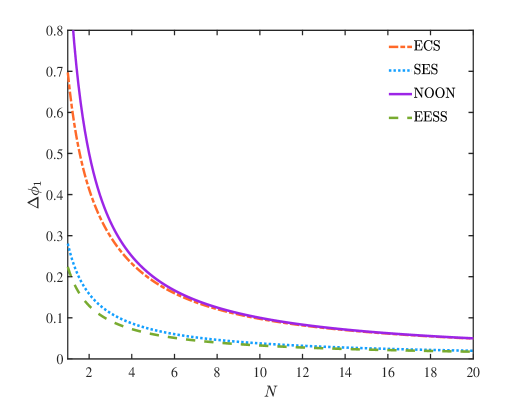
Fig. 2 shows the phase uncertainty $\Delta\phi_{\,1}$ for various quantum states varies with the average particle number $N$ in the lossless case. We find that when the average particle number is fixed, the ECS is superior to the NOON state only if $N$ is small, however, if we choose the SES as the input state, the precision is enhanced significantly regardless of the number of particles. To appreciate this, Eq. (19) is rewritten as

$$\left|\psi\right\rangle_{S}=\mathcal{N}_{\xi}\sum_{n=0}^{\infty}C_{2n}\left(\left|2n,0\right\rangle+\left|0,2n\right\rangle\right),$$ (22)

where $C_{2n}=1/\sqrt{\cosh r}\left(-e^{i\vartheta}\rm{tanh}r/2\right)^{n}\sqrt{(2n)!}/n!$, $\vartheta=\rm arg(\xi)$. It is easy to find that SES is a coherent superposition of the NOON states with different even numbers. It means larger particle number states are included in the SES than the ECS under the condition of the same average particle number, which is beneficial to improve the precision of the gyroscope.

Furthermore, Refs. Lee et al. (2016); Knott et al. (2016); Rubio and Dunningham (2019) show that the QFI is proportional to Mandel $\mathcal{Q}$-parameter of the single-mode in path-symmetric state, and in this article the QFI for parameter $\phi_{\,1}$ can be rewiritten as

$$F_{Q}=2N(\mathcal{Q}+1),$$ (23)

where $\mathcal{Q}=\Delta^{2}n_{1}/\left\langle n_{1}\right\rangle-1$, hence the squeezed vacuum state has an advantage over the coherent state for its super-Poissonian statistics.

Figure 2: Phase uncertainty $\Delta\phi_{\,1}$ varies with the number of particles in lossless case. $\Delta\phi_{\,1}$ of the NOON state (purple solid line) is approximately equal to that of the ECS (red dot-dashed line) for large $N$; $\Delta\phi_{1}$ of the EESS (green dashed line) is minimal in the low particle-number regime, however, when the particle number increases, the precision of the EESS is roughly equal to that of the SES.

III.4 Entangled even squeezed state

In the previous result, we reveal the relationship between the QFI and Mandel $\mathcal{Q}$-parameter, and one can immediately see that the states with larger Mandel $\mathcal{Q}$-parameters can give larger QFI. In general, the Mandel $\mathcal{Q}$ -parameter of the even coherent state is larger in comparision with the coherent state, and we follow this idea to consider the superpostion of two squeezed vacuum states, i.e.,

$$\left|\Phi\right\rangle=\mathcal{N}\left(\left|\xi\right\rangle+\left|-\xi\right\rangle\right),$$ (24)

where $\mathcal{N}=\left(2+2\left(\cosh 2r\right)^{-1\text{/2}}\right)^{-1/2},r=\left|\xi\right|$. Then we introduce the "entangled even squeezed state" (EESS) which is an original NOON-like state and constructed with $\left|\Phi\right\rangle$, that is

$$\left|\psi\right\rangle_{ES}=\mathcal{N}_{\Phi}\left(\left|\Phi,0\right\rangle+\left|0,\Phi\right\rangle\right)$$ (25)

where

$$\mathcal{N}_{\Phi}=\frac{\left(1+\left(\cosh 2r\right)^{-1\text{/2}}\right)^{1/2}}{\left[2+2\left(\cosh 2r\right)^{-1/2}+4\left(\cosh r\right)^{-1}\right]^{1/2}}.$$ (26)

Although $\left|\xi\right\rangle$ is an even state, the superposition shown in Eq. (24) can generate a more "even" state. The analytical expression of the QFI for parameter $\phi_{\,1}$ is presented in Appendix B, and the phase uncertainty $\Delta\phi_{\,1}$ of EESS with respect to $N$ is shown in Fig 2. We find the EESS has the best performance in the low-particle-number regime, but similar to the case of the NOON state and the ECS, the precision of the EESS and the SES tend to be the same as the average particle number increases. The specific explanation is presented in Appendix B. Then we set $\mathrm{arg}(\xi)=0$, and Eq. (25) can be expanded with Fock states, that is

$$\left|\psi\right\rangle_{ES}=\mathcal{N}_{\xi,-\xi}\sum_{m=0}^{\infty}D_{4m}\left(\left|4m,0\right\rangle+\left|0,4m\right\rangle\right),$$ (27)

where $D_{4m}=2\left(\cosh r\right)^{-1/2}\left(\tanh r/2\right)^{2m}\sqrt{\left(4m\right)!}/\left(2m\right)!$, $\mathcal{N}_{\xi,-\xi}=\mathcal{N}_{\Phi}\mathcal{N}$. Note that the EESS only involves number states that are multiples of four, and this leads to larger number states are included in the EESS than the SES for a fixed average particle number, which means larger QFI can be obtianed. Moreover, from Eq.(23) we see that the Mandel $\mathcal{Q}$-parameter of the single-mode component $\left|\Phi\right\rangle$ in the EESS determines the QFI directly. For a more specific example, taking $N=2$ and the $\mathcal{Q}$ for the SES is $\mathcal{Q}_{SES}\approx 9$, and $\mathcal{Q}_{EESS}\approx 14$ for the EESS. In Ref. Rubio and Dunningham (2019), the Mandel $\mathcal{Q}$-parameter for various states are given, and we see that the EESS has an even larger $\mathcal{Q}$ than the squeezed cat state ($\mathcal{Q}\approx 11.75$), which is considered as the optimal state in Ref. Knott et al. (2016). Additionally, $\phi_{+}$ and $\mathcal{N}_{\Phi}\left(\left|\Phi,\Phi\right\rangle+\left|0,0\right\rangle\right)$ can be employed to enhance the precision slightly, and in the large squeezing regime we can get the same result shown in Eq. (20).

IV EFFECTS OF PARTICLE LOSS

In practice, decoherence and particle loss are inevitable, thus it is necessary to take into account the effects of particle loss of the atomic gyroscope in this section. In Refs. Cooper et al. (2010); Zhang et al. (2013); Demkowicz-Dobrzanski et al. (2009), the related issues have been involved. In this paper, we still use the model that inserting two fictitious "beam splitter" with the transmission rate $\eta$ into two sites and, in general, the output state is described by a mixed state $\rho$. In this scheme, the particle loss is the loss from the momentum modes during $t_{\omega}$ Cooper et al. (2010). We assume that both modes have the same loss rates $R=1-\eta$, and the model in Ref. Demkowicz-Dobrzanski et al. (2009) is used here to describe the effect of particle loss on the QFI. The situations of the particle number state and the ECS have been discussed in Refs. Demkowicz-Dobrzanski et al. (2009); Joo et al. (2011); Zhang et al. (2013), thus we focus on the calculation of the SES and the EESS in this article, and more specific calculations are presented in Appendix C.

First of all, we should calculate the reduced density matrix of the SES after particle loss. The particle number states in Eq. (22) evolve into

$$\begin{split}\left|2n,0\right\rangle\rightarrow\sum_{l_{a}=0}^{2n}\sqrt{B_{l_{a}}^{2n}}\left|2n-l_{a},0\right\rangle\otimes\left|l_{a},0\right\rangle,\\ \left|0,2n\right\rangle\rightarrow\sum_{l_{b}=0}^{2n}\sqrt{B_{l_{b}}^{2n}}\left|0,2n-l_{b}\right\rangle\otimes\left|0,l_{b}\right\rangle,\end{split}$$ (28)

where

$$B_{l_{a(b)}}^{2n}=\left(\begin{array}[]{c}2n\\ l_{a(b)}\end{array}\right)\eta^{2n-l_{a(b)}}\left(1-\eta\right)^{l_{a(b)}},$$ (29)

and $\left|l_{a},0\right\rangle$ and $\left|0,l_{b}\right\rangle$ are the states which represent $l_{a},l_{b}$ particles are lost from site one and site two, respectively. Then we obtain the reduced density matrix which is expressed as

$$\rho=p_{0,0}\rho_{0,0}+\sum_{l_{a}=1}^{\infty}p_{l_{a},0}\rho_{l_{a},0}+\sum_{l_{b}=1}^{\infty}p_{0,l_{b}}\rho_{0,l_{b}},$$ (30)

where $\rho_{l,m}=\left|\psi_{l,m}\right\rangle\left\langle\psi_{l,m}\right|$, and $l,m$ are the number of particles lost. When $l=m=0$, we have

$$\left|\psi_{0,0}\right\rangle=\frac{1}{\sqrt{p_{0,0}}}\mathcal{N}_{\xi}\sum_{n=0}^{\infty}C_{2n}\eta^{n}\left(\left|2n,0\right\rangle+\left|0,2n\right\rangle\right).$$ (31)

Figure 3: Phase uncertainty $\Delta\phi_{\,1}$ varies with transmission rate $\eta$ for $N=2$. The green dashed line and the blue dotted line show the precision of $\phi_{\,1}$ for the EESS and the SES, respectively. The ECS and the NOON state which are investigated in the previous studies are depicted in red dot-dashed line and purple solid line for comparison.

While $l=l_{a},m=0$ and $l=0,m=l_{b}$, we also obtain

$$\begin{split}\left|\psi_{l_{a},0}\right\rangle=\frac{1}{\sqrt{p_{l_{a},0}}}\mathcal{N}_{\xi}\left(\sum_{n=\Gamma}^{\infty}C_{2n}\sqrt{B_{l_{a}}^{2n}}\left|2n-l_{a},0\right\rangle\right),\\ \left|\psi_{0,l_{b}}\right\rangle=\frac{1}{\sqrt{p_{0,l_{b}}}}\mathcal{N}_{\xi}\left(\sum_{n=\Gamma}^{\infty}C_{2n}\sqrt{B_{l_{b}}^{2n}}\left|0,2n-l_{b}\right\rangle\right),\end{split}$$ (32)

where

$$\Gamma=\begin{cases}\left(l_{a(b)}+1\right)/2&{\rm for}\ l_{a(b)}\rm\ is\ odd,\\ \ l_{a(b)}/2&{\rm for}\ l_{a(b)}\rm\ is\ even.\end{cases}$$ (33)

$p_{0,0}$, $p_{l_{a},0}$ and $p_{0,l_{b}}$ are the normalization factors required for calculation of the mixed state $\rho$. We set $\vartheta=0$, $\xi=r$, then Eq. (29) can be rewritten as

$$\left|\psi_{0,0}\right\rangle=\mathcal{N}_{\tilde{\xi}}\left(\left|\tilde{r},0\right\rangle+\left|0,\tilde{r}\right\rangle\right),$$ (34)

where $\tilde{r}=\mathrm{arc}\tanh\left(\eta\tanh r\right)$, and $\mathcal{N}_{\tilde{\xi}}=\left(2/\cosh\tilde{r}+2\right)^{-1/2}$. Utilizing Eqs. (31), (32), (34) and the normalized property of states, we can obtain

$$\begin{split}&p_{0,0}=\frac{1+\cosh\tilde{r}}{1+\cosh r},\\ \sum_{l_{a}=1}^{\infty}&p_{l_{a},0}=\sum_{l_{b}=1}^{\infty}p_{0,l_{b}}=\frac{\cosh r-\cosh\tilde{r}}{2\left(1+\cosh r\right)}.\end{split}$$ (35)

To obtain the QFI of the mixed state $\rho$, we have to diagonalize the mixed state as $\rho=\sum_{m}\lambda_{m}\left|\lambda_{m}\right\rangle\left\langle\lambda_{m}\right|$, where $\lambda_{m}$ is an eigenvalue and $\left|\lambda_{m}\right\rangle$ is eigenvector. Here we first estimate the phase $\theta$ through $\phi_{\,1}$, then choose average particle number $N=2$, and then truncate the particle number state at $n=56$ in Eq. (31). For a mixed state $\rho$, the QFI is expressed as Liu et al. (2014a, b); Yu et al. (2018)

$$F_{Q}=4\sum_{m}\lambda_{m}\left\langle\lambda_{m}\right|n_{1}^{2}\left|\lambda_{m}\right\rangle-\sum_{m,m^{\prime}}\frac{8\lambda_{m}\lambda_{m^{\prime}}}{\lambda_{m}+\lambda_{m^{\prime}}}\left|\left\langle\lambda_{m}\right|n_{1}\left|\lambda_{m^{\prime}}\right\rangle\right|^{2},$$ (36)

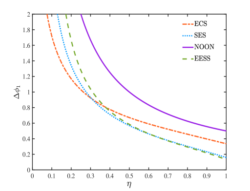
and the numerical simulation of QFI is shown in Fig. 3. Here we give the specific calculation of the SES, and the case of the EESS is very similar so we put it into Appendix C.

In Fig. 3 we present the variation of $\Delta\phi_{\,1}$ with the change of $\eta$. In the low loss regime, the EESS gives the best precision compared with the SES state, the ECS, and the NOON state. This advantage in precision persists until $\eta<0.5$, and is inferior to the ECS when $\eta<0.37$. In general, the loss rates in an experiment is smaller than $50\%$ Cooper et al. (2010), and thus the EESS is the preferred state to obtain the maximum precision.

V CONCLUSION

In this paper, we have investigated the optimal input state in the atomic gyroscope which is based on three-site Bose-Hubbard model, and the main approach is to find the state that has the maximal QFI. We have provided a Hermitian operator $\mathcal{H}$ which contains the dynamical information of the whole process, hence the measurement procedure can be simplified as an equivalent unitary transformation. To obtain the maximal QFI, we take the squeezed entangled state (SES) and the entangled even squeezed state (EESS) as candidates to improve the precision of the atomic gyroscope.

Compared with the particle number state (especially the NOON state) and the entangled coherent state, the best precision is achieved by taking the EESS as the input state in the ideal case. In addition, the existence of an extra mode allows us to set up a phase reference, which can make it possible to estimate the phase change of a mode directly. And on this basis, we found that using another form of entangled states, such as $\left|\psi\right\rangle_{M}$, $\left|\psi\right\rangle_{EM}$ and $\left|\psi\right\rangle_{SM}$ can obtain slightly better precision in the lossless case. Moreover, the QFI under practical conditions is also considered, and we found that the EESS improve the precision significantly in moderate loss regime. Although we face some challenges that there is no current experimental scheme or technology is proposed to generate the EESS, it is still the preferred input state in this measurement scheme. And the results we obtained in this article also fully demonstrate the EESS has a great potential in quantum metrology. Furthermore, we believe that the method we used in this article is helpful to the people who want to improve the precision of other measurement systems.

Appendix A THE DERIVATION OF $\mathcal{H}$

First, we know that step (ii) to (vi) can be regarded as unitary transformations, and we use $\left\{U_{2}...U_{6}\right\}$ to represent step (ii)-(vi). For a pure state, the QFI with respect to parameter $\theta$ is given by

$$F_{Q}=4\left(\left\langle\partial_{\theta}\psi|\partial_{\theta}\psi\right\rangle-\left|\left\langle\psi|\partial_{\theta}\psi\right\rangle\right|^{2}\right).$$ (37)

In step (i) an initial state $\left|\psi\right\rangle_{\rm in}$ is prepared, and $\left|\psi\right\rangle=U_{6}U_{5}...U_{2}\left|\psi\right\rangle_{\rm in}=\prod_{i=2}^{6}U_{8-i}\left|\psi\right\rangle_{\rm in}$. Note that only $U_{4}$ is the function of $\theta$, and utilizing Eq. (2) the QFI with respect with $\theta$ is express as

$$\begin{split}F_{Q}&=4\left({}_{\rm in}\!\left\langle\psi\right|U_{2}^{\dagger}U_{3}^{\dagger}\mathcal{H}_{4}^{2}U_{3}U_{2}\left|\psi\right\rangle_{\rm in}-\left|{}_{\rm in}\!\left\langle\psi\right|U_{2}^{\dagger}U_{3}^{\dagger}\mathcal{H}_{4}U_{3}U_{2}\left|\psi\right\rangle_{\rm in}\right|^{2}\right)\\ &=4\left({}_{\rm in}\!\left\langle\psi\right|\mathcal{H}^{2}\left|\psi\right\rangle_{\rm in}-\left|{}_{\rm in}\!\left\langle\psi\right|\mathcal{H}\left|\psi\right\rangle_{\rm in}\right|^{2}\right)\end{split}$$ (38)

where $U_{4}=e^{-iH_{r}t_{\omega}/\hbar}$,$\mathcal{H}_{4}=i\left(\partial_{\theta}U_{4}^{\dagger}\right)U_{4}=-\partial_{\theta}H_{r}t_{\omega}/\hbar$, and the equality $\left(\partial_{\theta}U^{\dagger}\right)U=-U^{\dagger}\left(\partial_{\theta}U\right)$ is used here. The specific expression of $\mathcal{H}_{4}$ is given by

$$\begin{split}\mathcal{H}_{4}&=\frac{-2Jt_{\omega}}{3}\left[\sin\left(\frac{\theta+2\pi}{3}\right)n_{-1}^{\alpha}+\sin\left(\frac{\theta}{3}\!\right)n_{0}^{\alpha}+\sin\left(\frac{\theta-2\pi}{3}\right)n_{1}^{\alpha}\right]\\ &=\frac{iJt_{\omega}}{3}e^{\frac{i\theta}{3}}\left(a_{0}^{\dagger}a_{1}+a_{1}^{\dagger}a_{2}+a_{2}^{\dagger}a_{0}\right)+h.c.,\end{split}$$ (39)

where $n_{j}^{\alpha}=\alpha_{j}^{\dagger}\alpha_{j}$, $j=-1,0,1$, and Eq. (5) is used to obtain the second line of Eq. (39). In order to obtain $\mathcal{H}$, we have

$$U_{3}^{\dagger}\mathcal{H}_{4}U_{3}=\frac{iJt_{\omega}}{3}e^{\frac{i\theta}{3}}\left(a_{0}^{\dagger}a_{1}+a_{1}^{\dagger}a_{2}e^{-i\frac{4\pi}{3}}+a_{2}^{\dagger}a_{0}e^{i\frac{4\pi}{3}}\right)+h.c.$$ (40)

Then we use quasi-momentum basis in the following calculation, and Eq. (40) becomes

$$U_{3}^{\dagger}\mathcal{H}_{4}U_{3}=\frac{iJt_{\omega}}{3}e^{\frac{i\theta}{3}}\left(\alpha_{-1}^{\dagger}\alpha_{0}+\alpha_{0}^{\dagger}\alpha_{1}e^{-i\frac{2\pi}{3}}+\alpha_{1}^{\dagger}\alpha_{-1}e^{i\frac{2\pi}{3}}\right)+h.c.,$$ (41)

and $U_{2}$ in Eq. (II) is expressed as

$$U_{2}=e^{i\frac{2\pi}{9}\left(2\alpha_{0}^{\dagger}\alpha_{0}-\alpha_{-1}^{\dagger}\alpha_{-1}-\alpha_{1}^{\dagger}\alpha_{1}\right)}.$$ (42)

Utilizing Eqs. (41) and (42), we have

$$\begin{split}\mathcal{H}&=U_{2}^{\dagger}U_{3}^{\dagger}\mathcal{H}_{4}U_{3}U_{2}\\ &=\frac{iJt_{\omega}}{3}e^{i\frac{\left(\theta+2\pi\right)}{3}}\left(\alpha_{-1}^{\dagger}\alpha_{0}+\alpha_{0}^{\dagger}\alpha_{1}+\alpha_{1}^{\dagger}\alpha_{-1}\right)+h.c.\end{split}$$ (43)

Finally, we utilize the initial basis $\left(a_{0},a_{1},a_{2}\right)^{\rm T}$ and obtain Eq. (9)

$$\mathcal{H}=-\frac{2Jt_{\omega}}{3}\left[\sin\left(\frac{\theta+2\pi}{3}\right)n_{0}+\sin\left(\frac{\theta\!-2\pi}{3}\right)n_{1}+\sin\left(\frac{\theta}{3}\right)n_{2}\right].$$ (44)

Appendix B THE ANALYTICAL EXPRESSION OF THE QFI OF THE ESES

To obtain the QFI of the EESS with respect to parameter $\phi_{\,1}$, we need to calculate $\Delta^{2}n_{1}$. For a squeezed vacuum state $\left|\xi\right\rangle=S(\xi)\left|0\right\rangle$, we have

$$\left\langle\xi|-\xi\right\rangle=\frac{1}{\sqrt{\cosh 2r}},$$ (45)

$$\left\langle\xi|a^{\dagger}a|-\xi\right\rangle=-\frac{\sinh^{2}r}{\left(\cosh 2r\right)^{3/2}},$$ (46)

$$\left\langle\xi\right|a^{\dagger}aa^{\dagger}a\left|-\xi\right\rangle=-\frac{\left(3+\cosh 2r\right)\sinh^{2}r}{2\left(\cosh 2r\right)^{5/2}}$$ (47)

and here we set $\rm arg(\xi)=0$. It is known that $\Delta^{2}n_{1}=_{ES}\!\!\left\langle\psi|n_{1}^{2}|\psi\right\rangle\!_{ES}-\left|{}_{ES}\!\left\langle\psi|n_{1}|\psi\right\rangle\!_{ES}\right|^{2}$, and the first term of the right side is

$$\left\langle n_{1}^{2}\right\rangle=2\mathcal{N}_{\xi,-\xi}^{2}\left(2\sinh^{2}r\cosh^{2}r+\!\sinh^{4}r-\frac{\left(3+\cosh 2r\right)\sinh^{2}r}{2\left(\cosh 2r\right)^{5/2}}\right),$$ (48)

and the second term is

$$\begin{split}\left\langle n_{1}\right\rangle^{2}&=4\mathcal{N}_{\xi,-\xi}^{4}\sinh^{4}r\left(1-\left(\cosh 2r\right)^{-3/2}\right)^{2}\\ &=\frac{N^{2}}{4}\end{split}$$ (49)

where $\mathcal{N}_{\xi,-\xi}=\left(1+(\cosh 2r)^{-1/2}+2(\cosh r)^{-1}\right)^{-1/2}/2$. The second line of Eq. (49) is because the total average particle number is $N$. Finally, the QFI of the EESS is give by

$$\begin{split}F_{Q}(\phi_{\,1})&=\frac{2N\left(2\cosh^{2}r+\sinh^{2}r-\frac{\left(3+\cosh 2r\right)}{2\left(\cosh 2r\right)^{5/2}}\right)}{1-\left(\cosh 2r\right)^{-3/2}}-N^{2}\\ &=N\left(\frac{3+3(\cosh 2r)^{2}+\cosh 2r}{\cosh 2r}+\frac{3\left(\cosh 2r\right)^{1/2}}{1+\left(\cosh 2r\right)^{1/2}+\cosh 2r}-N\right)\end{split}$$ (50)

In the large squeezing regime $r\gg 1$, we have $\mathcal{N}_{\xi,-\xi}\approx 1/2$, $\sinh^{2}r=(\cosh 2r-1)/2\approx N$, and $F_{Q}$ becomes

$$F_{Q}(\phi_{\,1})\approx 5N^{2}+4N.$$ (51)

This result shows that the QFI of the EESS is approximately equal to that of the SES under condition of large $N$.

Appendix C PARTICLE LOSS OF THE ESES

In this Appendix, we give a specific approach to calculate the effect of particle loss of the EESS. The reduced density matrix of the EESS is expressed as

$$\bar{\rho}=\bar{p}_{0,0}\bar{\rho}_{0,0}+\sum_{l_{a}=1}^{\infty}\bar{p}_{l_{a},0}\bar{\rho}_{l_{a},0}+\sum_{l_{b}=1}^{\infty}\bar{p}_{0,l_{b}}\bar{\rho}_{0,l_{b}},$$ (52)

where $\bar{\rho}_{l,m}=\left|\bar{\psi}_{l,m}\right\rangle\left\langle\bar{\psi}_{l,m}\right|$, and $l,m$ are the number of particles lost. Similar to Eqs. (31) and (32), we have

$$\left|\bar{\psi}_{0,0}\right\rangle=\frac{1}{\sqrt{\bar{p}_{0,0}}}\mathcal{N}_{\xi,-\xi}\sum_{n=0}^{\infty}D_{4m}\eta^{2m}\left(\left|4m,0\right\rangle+\left|0,4m\right\rangle\right),$$ (53)

and

$$\begin{split}\left|\bar{\psi}_{l_{a},0}\right\rangle=\frac{1}{\sqrt{\bar{p}_{l_{a},0}}}\mathcal{N}_{\xi,-\xi}\left(\sum_{\{m|4m\geq l_{a},m\in z\}}\!\!\!\!\!\!\!\!\!\!\!\!\!\!D_{4m}\sqrt{B_{l_{a}}^{4m}}\left|4m-l_{a},0\right\rangle\right),\\ \left|\bar{\psi}_{0,l_{b}}\right\rangle=\frac{1}{\sqrt{\bar{p}_{0,l_{b}}}}\mathcal{N}_{\xi,-\xi}\left(\sum_{\{m|4m\geq l_{b},m\in z\}}\!\!\!\!\!\!\!\!\!\!\!\!\!\!D_{4m}\sqrt{B_{l_{b}}^{4m}}\left|0,4m-l_{b}\right\rangle\right),\end{split}$$ (54)

where $\bar{p}_{0,0}$, $\bar{p}_{l_{a},0}$ and $\bar{p}_{0,l_{b}}$ are the normalization factors. To obtain these three factors, $D_{4m}\eta^{2m}$ in Eq. (53) can be written as

$$\begin{split}D_{4m}\eta^{2m}&=\frac{2}{\sqrt{\cosh r}}\left(\frac{1}{2}\eta\tanh r\right)^{2m}\frac{\sqrt{(4m)!}}{(2m)!}\\ &=\sqrt{\frac{\cosh\tilde{r}}{\cosh r}}\frac{2}{\sqrt{\cosh\tilde{r}}}\left(\frac{1}{2}\tanh\tilde{r}\right)^{2m}\frac{\sqrt{(4m)!}}{(2m)!}\\ &=\sqrt{\frac{\cosh\tilde{r}}{\cosh r}}\widetilde{D}_{4m},\end{split}$$ (55)

where $\tilde{r}=\rm arctanh(\eta\tanh r)$. Then we rewrite Eq. (53) as

$$\begin{split}\left|\bar{\psi}_{0,0}\right\rangle&=\frac{1}{\sqrt{\bar{p}_{0,0}}}\mathcal{N}_{\xi,-\xi}\sum_{n=0}^{\infty}D_{4m}\eta^{2m}\left(\left|4m,0\right\rangle+\left|0,4m\right\rangle\right)\\ &=\frac{1}{\sqrt{\bar{p}_{0,0}}}\sqrt{\frac{\cosh\tilde{r}}{\cosh r}}\frac{\mathcal{N}_{\Phi}\mathcal{N}}{\widetilde{\mathcal{N}}}\sum_{m=0}^{\infty}\widetilde{D}_{4m}\widetilde{\mathcal{N}}\left(\left|4m,0\right\rangle+\left|0,4m\right\rangle\right)\\ &=\mathcal{N}_{\tilde{\Phi}}\left(\left|\tilde{\Phi},0\right\rangle+\left|0,\tilde{\Phi}\right\rangle\right)\end{split}$$ (56)

where $\widetilde{\mathcal{N}}=\left(2+2\left(\cosh 2\tilde{r}\right)^{-1\text{/2}}\right)^{-1/2}$, $\left|\tilde{\Phi}\right\rangle=\mathcal{N}\left(\left|\tilde{r}\right\rangle+\left|-\tilde{r}\right\rangle\right)$, and

$$\mathcal{N}_{\tilde{\Phi}}=\frac{\left(1+\left(\cosh 2\tilde{r}\right)^{-1/2}\right)^{1/2}}{\left[2+2\left(\cosh 2\tilde{r}\right)^{-1/2}+4\left(\cosh\tilde{r}\right)^{-1}\right]^{1/2}}.$$ (57)

Note that we set $\arg(\xi)=0$ here. From Eqs. (56) and (57), we can obtain

$$\bar{p}_{0,0}=\frac{\mathcal{N}^{2}}{\mathcal{\widetilde{N}}^{2}}\frac{\cosh\tilde{r}}{\cosh r}\frac{\mathcal{N}_{\Phi}^{2}}{\mathcal{N}_{\tilde{\Phi}}^{2}}.$$ (58)

For $\bar{p}_{l_{a},0}$ and $\bar{p}_{0,l_{b}}$, we have

$$\begin{split}\sum_{l_{a}=1}^{\infty}\bar{p}_{l_{a},0}&=\sum_{l_{b}=1}^{\infty}\bar{p}_{0,l_{b}}\\ &={\sum_{l_{a}=0}^{\infty}}\mathcal{N}_{\Phi}^{2}\mathcal{N}^{2}\!\!\!\!\!\!\!\!\!\!\!\!\!\sum_{\{m|4m\geq l_{a},m\in z\}}\!\!\!\!\!\!\!\!\!\!\!\!\!D_{4m}^{2}B_{l_{a}}^{4m}-\mathcal{N}_{\Phi}^{2}\mathcal{N}^{2}\sum_{m=0}^{\infty}D_{4m}^{2}B_{0}^{4m}\\ &=\mathcal{N}_{\Phi}^{2}\left(1-\frac{\cosh\tilde{r}}{\cosh r}\frac{\mathcal{N}^{2}}{\mathcal{\widetilde{N}}^{2}}\right).\end{split}$$ (59)

In fact, $\bar{p}_{l,m}$ is the probability of the density matrix with the corresponding particle loss. And utilizing the relationship between $\mathcal{N}_{\Phi}$ and $\mathcal{N}_{\tilde{\Phi}}$

$$\frac{\mathcal{N}^{2}\cosh\tilde{r}}{\mathcal{\widetilde{N}}^{2}\cosh r}\left(\frac{1-2\mathcal{N}_{\tilde{\Phi}}^{2}}{\mathcal{N}_{\tilde{\Phi}}^{2}}\right)=\frac{1-2\mathcal{N}_{\Phi}^{2}}{\mathcal{N}_{\Phi}^{2}},$$ (60)

It’s easy to verify that $p_{0,0}+\sum_{l_{a}=1}^{\infty}\bar{p}_{l_{a},0}+\sum_{l_{b}=1}^{\infty}\bar{p}_{0,l_{b}}=1$.

References

- Taylor and Bowen (2016) M. A. Taylor and W. P. Bowen, Quantum metrology and its application in biology, Physics Reports 615, 1 (2016), quantum metrology and its application in biology.
- Taylor et al. (2013) M. A. Taylor, J. Janousek, V. Daria, J. Knittel, B. Hage, H.-A. Bachor, and W. P. Bowen, Biological measurement beyond the quantum limit, Nature Photonics 7, 229 (2013).
- Nasr et al. (2009) M. B. Nasr, D. P. Goode, N. Nguyen, G. Rong, L. Yang, B. M. Reinhard, B. E. Saleh, and M. C. Teich, Quantum optical coherence tomography of a biological sample, Optics Communications 282, 1154 (2009).
- Morris et al. (2015) P. A. Morris, R. S. Aspden, J. E. C. Bell, R. W. Boyd, and M. J. Padgett, Imaging with a small number of photons, Nature Communications 6, 5913 (2015).
- Fixler et al. (2007) J. B. Fixler, G. T. Foster, J. M. McGuirk, and M. A. Kasevich, Atom interferometer measurement of the newtonian constant of gravity, Science 315, 74 (2007), https://science.sciencemag.org/content/315/5808/74.full.pdf .
- Hu et al. (2013) Z.-K. Hu, B.-L. Sun, X.-C. Duan, M.-K. Zhou, L.-L. Chen, S. Zhan, Q.-Z. Zhang, and J. Luo, Demonstration of an ultrahigh-sensitivity atom-interferometry absolute gravimeter, Phys. Rev. A 88, 043610 (2013).
- Lamporesi et al. (2008) G. Lamporesi, A. Bertoldi, L. Cacciapuoti, M. Prevedelli, and G. M. Tino, Determination of the newtonian gravitational constant using atom interferometry, Phys. Rev. Lett. 100, 050801 (2008).
- Demkowicz-Dobrzański et al. (2013) R. Demkowicz-Dobrzański, K. Banaszek, and R. Schnabel, Fundamental quantum interferometry bound for the squeezed-light-enhanced gravitational wave detector geo 600, Phys. Rev. A 88, 041802 (2013).
- Purdy et al. (2013) T. P. Purdy, R. W. Peterson, and C. A. Regal, Observation of radiation pressure shot noise on a macroscopic object, Science 339, 801 (2013), https://science.sciencemag.org/content/339/6121/801.full.pdf .
- Punturo et al. (2010) M. Punturo, M. Abernathy, F. Acernese, B. Allen, N. Andersson, K. Arun, F. Barone, B. Barr, M. Barsuglia, M. Beker, et al., The third generation of gravitational wave observatories and their science reach, Classical and Quantum Gravity 27, 084007 (2010).
- Braginsky and Vyatchanin (2004) V. Braginsky and S. Vyatchanin, Corner reflectors and quantum-non-demolition measurements in gravitational wave antennae, Physics Letters A 324, 345 (2004).
- Adhikari (2014) R. X. Adhikari, Gravitational radiation detection with laser interferometry, Rev. Mod. Phys. 86, 121 (2014).
- McGuirk et al. (2002) J. M. McGuirk, G. T. Foster, J. B. Fixler, M. J. Snadden, and M. A. Kasevich, Sensitive absolute-gravity gradiometry using atom interferometry, Phys. Rev. A 65, 033608 (2002).
- Caves (1981) C. M. Caves, Quantum-mechanical noise in an interferometer, Phys. Rev. D 23, 1693 (1981).
- Dorner et al. (2009) U. Dorner, R. Demkowicz-Dobrzanski, B. J. Smith, J. S. Lundeen, W. Wasilewski, K. Banaszek, and I. A. Walmsley, Optimal quantum phase estimation, Phys. Rev. Lett. 102, 040403 (2009).
- Lee et al. (2002) H. Lee, P. Kok, and J. P. Dowling, A quantum rosetta stone for interferometry, Journal of Modern Optics 49, 2325 (2002).
- Cooper et al. (2010) J. J. Cooper, D. W. Hallwood, and J. A. Dunningham, Entanglement-enhanced atomic gyroscope, Phys. Rev. A 81, 043624 (2010).
- Tsarev et al. (2018) D. V. Tsarev, S. M. Arakelian, Y.-L. Chuang, R.-K. Lee, and A. P. Alodjants, Quantum metrology beyond heisenberg limit with entangled matter wave solitons, Opt. Express 26, 19583 (2018).
- Joo et al. (2011) J. Joo, W. J. Munro, and T. P. Spiller, Quantum metrology with entangled coherent states, Phys. Rev. Lett. 107, 083601 (2011).
- Joo et al. (2012) J. Joo, K. Park, H. Jeong, W. J. Munro, K. Nemoto, and T. P. Spiller, Quantum metrology for nonlinear phase shifts with entangled coherent states, Phys. Rev. A 86, 043828 (2012).
- Zhang et al. (2013) Y. M. Zhang, X. W. Li, W. Yang, and G. R. Jin, Quantum fisher information of entangled coherent states in the presence of photon loss, Phys. Rev. A 88, 043832 (2013).
- Liu et al. (2016) J. Liu, X.-M. Lu, Z. Sun, and X. Wang, Quantum multiparameter metrology with generalized entangled coherent state, Journal of Physics A: Mathematical and Theoretical 49, 115302 (2016).
- Arditty and Lefèvre (1981) H. J. Arditty and H. C. Lefèvre, Sagnac effect in fiber gyroscopes, Opt. Lett. 6, 401 (1981).
- Gustavson et al. (1997) T. L. Gustavson, P. Bouyer, and M. A. Kasevich, Precision rotation measurements with an atom interferometer gyroscope, Phys. Rev. Lett. 78, 2046 (1997).
- Kasevich and Chu (1992) M. Kasevich and S. Chu, Measurement of the gravitational acceleration of an atom with a light-pulse atom interferometer, Applied Physics B 54, 321 (1992).
- Gustavson et al. (2000) T. L. Gustavson, A. Landragin, and M. A. Kasevich, Rotation sensing with a dual atom-interferometer sagnac gyroscope, Classical and Quantum Gravity 17, 2385 (2000).
- Wu et al. (2007) S. Wu, E. Su, and M. Prentiss, Demonstration of an area-enclosing guided-atom interferometer for rotation sensing, Phys. Rev. Lett. 99, 173201 (2007).
- Alzar et al. (2012) C. L. G. Alzar, W. Yan, and A. Landragin, Towards high sensitivity rotation sensing using an atom chip, in Research in Optical Sciences (Optical Society of America, 2012) p. JT2A.10.
- Stevenson et al. (2015) R. Stevenson, M. R. Hush, T. Bishop, I. Lesanovsky, and T. Fernholz, Sagnac interferometry with a single atomic clock, Phys. Rev. Lett. 115, 163001 (2015).
- Rico-Gutierrez et al. (2015) L. M. Rico-Gutierrez, T. P. Spiller, and J. A. Dunningham, Quantum-enhanced gyroscopy with rotating anisotropic bose–einstein condensates, New Journal of Physics 17, 043022 (2015).
- Cooper et al. (2009) J. J. Cooper, D. W. Hallwood, and J. A. Dunningham, Scheme for implementing atomic multiport devices, Journal of Physics B: Atomic, Molecular and Optical Physics 42, 105301 (2009).
- Helstrom (1976) C. W. Helstrom, Quantum detection and estimation theory (Academic, New York, 1976).
- Braunstein and Caves (1994) S. L. Braunstein and C. M. Caves, Statistical distance and the geometry of quantum states, Phys. Rev. Lett. 72, 3439 (1994).
- Holevo (1982) A. S. Holevo, Probabilistic and Statistical Aspects of Quantum Theory (North-Holland, Amsterdam, 1982).
- Braunstein et al. (1996) S. L. Braunstein, C. M. Caves, and G. Milburn, Generalized uncertainty relations: Theory, examples, and lorentz invariance, Annals of Physics 247, 135 (1996).
- Liu et al. (2019) J. Liu, H. Yuan, X.-M. Lu, and X. Wang, Quantum fisher information matrix and multiparameter estimation, Journal of Physics A: Mathematical and Theoretical 53, 023001 (2019).
- Pang and Brun (2014) S. Pang and T. A. Brun, Quantum metrology for a general hamiltonian parameter, Phys. Rev. A 90, 022117 (2014).
- Liu et al. (2015) J. Liu, X.-X. Jing, and X. Wang, Quantum metrology with unitary parametrization processes, Scientific Reports 5, 8565 (2015).
- Jing et al. (2015) X.-X. Jing, J. Liu, H.-N. Xiong, and X. Wang, Maximal quantum fisher information for general su(2) parametrization processes, Phys. Rev. A 92, 012312 (2015).
- Huver et al. (2008) S. D. Huver, C. F. Wildfeuer, and J. P. Dowling, Entangled fock states for robust quantum optical metrology, imaging, and sensing, Phys. Rev. A 78, 063828 (2008).
- Knott et al. (2016) P. A. Knott, T. J. Proctor, A. J. Hayes, J. P. Cooling, and J. A. Dunningham, Practical quantum metrology with large precision gains in the low-photon-number regime, Phys. Rev. A 93, 033859 (2016).
- Lee et al. (2016) S.-Y. Lee, C.-W. Lee, J. Lee, and H. Nha, Quantum phase estimation using path-symmetric entangled states, Scientific Reports 6, 30306 (2016).
- Rubio and Dunningham (2019) J. Rubio and J. Dunningham, Quantum metrology in the presence of limited data, New Journal of Physics 21, 043037 (2019).
- Hallwood et al. (2007) D. W. Hallwood, K. Burnett, and J. Dunningham, The barriers to producing multiparticle superposition states in rotating bose–einstein condensates, Journal of Modern Optics 54, 2129 (2007), https://doi.org/10.1080/09500340701427128 .
- Dunningham et al. (2012) J. A. Dunningham, J. J. Cooper, and D. W. Hallwood, Quantum metrology with rotating matter waves in different geometries, AIP Conference Proceedings 1469, 23 (2012), https://aip.scitation.org/doi/pdf/10.1063/1.4746058 .
- Hallwood et al. (2006) D. W. Hallwood, K. Burnett, and J. Dunningham, Macroscopic superpositions of superfluid flows, New Journal of Physics 8, 180 (2006).
- Jarzyna and Demkowicz-Dobrzański (2012) M. Jarzyna and R. Demkowicz-Dobrzański, Quantum interferometry with and without an external phase reference, Phys. Rev. A 85, 011801 (2012).
- Demkowicz-Dobrzanski et al. (2009) R. Demkowicz-Dobrzanski, U. Dorner, B. J. Smith, J. S. Lundeen, W. Wasilewski, K. Banaszek, and I. A. Walmsley, Quantum phase estimation with lossy interferometers, Phys. Rev. A 80, 013825 (2009).
- Liu et al. (2014a) J. Liu, X.-X. Jing, W. Zhong, and X.-G. Wang, Quantum fisher information for density matrices with arbitrary ranks, Communications in Theoretical Physics 61, 45 (2014a).
- Liu et al. (2014b) J. Liu, H.-N. Xiong, F. Song, and X. Wang, Fidelity susceptibility and quantum fisher information for density operators with arbitrary ranks, Physica A: Statistical Mechanics and its Applications 410, 167 (2014b).
- Yu et al. (2018) X. Yu, X. Zhao, L. Shen, Y. Shao, J. Liu, and X. Wang, Maximal quantum fisher information for phase estimation without initial parity, Opt. Express 26, 16292 (2018).