A fundamental problem of hypothesis testing with finite inventory in e-commerce

Abstract.

In this paper, we draw attention to a problem that is often overlooked or ignored by companies practicing hypothesis testing (A/B testing) in online environments. We show that conducting experiments on limited inventory that is shared between variants in the experiment can lead to high false positive rates since the core assumption of independence between the groups is violated. We provide a detailed analysis of the problem in a simplified setting whose parameters are informed by realistic scenarios. The setting we consider is a $2$-dimensional random walk in a semi-infinite strip. It is rich enough to take a finite inventory into account, but is at the same time simple enough to allow for a closed form of the false-positive probability. We prove that high false-positive rates can occur, and develop tools that are suitable to help design adequate tests in follow-up work. Our results also show that high false-negative rates may occur. The proofs rely on a functional limit theorem for the $2$-dimensional random walk in a semi-infinite strip.

1. Introduction

The golden standard for testing product changes on e-commerce websites is large scale hypothesis testing also known as A/B-Testing.

When a given version of a website is modified, it is natural to ask whether or not the modified (new) version of the website performs better than the old one. It is very common to use the following approach based on classic hypothesis testing:

During a fixed time period, the so-called testing phase, whenever customers visit the website, they are displayed one of the two versions of it, where the choice which one they get to see is random. For each version of the website the owner thus collects a sample containing for each customer visiting that website relevant data such as whether or not they bought a good or how much money was spent by the customers, etc. Then a statistical test (A/B test) is applied to evaluate which version of the website performed better.

Typically, these tests rely on the assumption of independent samples. In the present paper, we point out in a quantitative way that in the situation where there is a finite amount of a popular good the independence assumption is not feasible and can often lead to wrong conclusions. The inventory is shared between variants and if a copy of an item is sold it can not be bought by users that enter the experiment later. This implies that users are not independent both inside as well as between the variants. These dependencies could be avoided by randomly splitting on an item level instead of a user level, but this would reduce the choice of the customer and is therefore not a realistic setup.

We think it is best to illustrate the dependence problem with a ranking example that we will use throughout the paper. We limit ourselves to only two distinct products (which each should be thought of as a variety of different products grouped into one). Using realistic parameters we show that two different ranking algorithms which perform identical if run independently show a significant difference almost 20% of the time when run in an industry standard A/B experiment. We also show that if there is a difference in performance between the algorithms there are scenarios where the power of a standard A/B test is close to 0.

Example 1.1 (Ranking experiment, take 1).

We consider a ranking experiment with two types of goods, one rare good, which is very attractive (good $2$), and a second, less attractive good (good $1$) available in practically unlimited quantities. In applications, there may be more than two types of goods, but the less attractive ones are labeled as type-$1$ goods, while the most attractive ones are labeled as type-$2$ goods. Suppose that in total there are $1\,000$ goods of type $2$ and $1\,000\,000$ goods of type $1$.

A website displays the available goods to each visitor. The goods are displayed in a certain order, which depends on the ranking algorithm used. The owner of the website wants to compare two different algorithms. The default algorithm, Algorithm $0$, displays the goods such that the type-$2$ goods have a low ranking and appear late in the list. Thus, only a fraction of the visitors gets to see them. The new algorithm, Algorithm $1$, displays the goods such that the type-$2$ goods have the highest ranking and appear first in the list. Every visitor seeing the goods ranked by Algorithm $1$ will see both, type-$1$ and type-$2$ goods (as long as they are available). The goal is to find out which of the two algorithms leads to a higher overall conversion rate, i.e., to a higher empirical probability to make a sale.

Suppose that during a test phase, $n=4\,000\,000$ customers visit the website. Whenever a customer visits the website, a fair coin is tossed. If the coin shows heads, the products are displayed ranked according to Algorithm $1$, if the coin shows tails, the products are displayed ranked according to Algorithm $0$.

We now make the following model assumptions. We assume that, independent of all other customers, each customer has a chance of $20\%$ of preferring good $1$ over good $2$ and an $80\%$ chance of preferring good $2$ over good $1$. When the goods are ranked according to Algorithm $0$, the customer first sees type-$1$ goods. There is a $5\%$ chance that the customer scrolls down and spots a type-$2$ good (if still available). A customer who sees both goods and has a preference for good $2$ will buy good $2$ with $10\%$ chance and will not buy at all with $90\%$ chance. A customer who either sees both goods and has a preference for good $1$ or sees only good $1$ will buy good $1$ with a $5\%$ chance and will not make a buy at all with $95\%$ chance. For simplicity, we assume that each customer buys at most one good.

Figure 1. Ranking experiment: Algorithm 0

Figure 2. Ranking experiment: Algorithm 1

The data collected is a sample $(x_{1},y_{1},i_{1}),\ldots,(x_{n},y_{n},i_{n})$ where $n$ is the sample size, i.e., the number of customers visiting the website during a certain test period. Here, $i_{k}$ is either $0$ or $1$, depending on whether Algorithm $0$ or $1$ was used to display the goods to the $k^{\rm th}$ customer. Further, $x_{k}=1$ or $x_{k}=0$ depending on whether good 1 was bought or not and, analogously, $y_{k}=1$ or $y_{k}=0$ depending on whether good 2 was bought or not. Notice that by our assumption that each customer buys at most one good, we have $x_{k}+y_{k}\in\{0,1\}$. Those $(x_{k},y_{k},i_{k})$ with $i_{k}=0$ are assigned to sample $0$ and the others to sample $1$. We write $n_{0}\vcentcolon=\sum_{k=1}^{n}(1-i_{k})$ and $n_{1}\vcentcolon=\sum_{k=1}^{n}i_{k}$ for the corresponding sample sizes. The numbers of sales in each group are $\ell_{0}=\sum_{k=1}^{n}(x_{k}+y_{k})(1-i_{k})$ and $\ell_{1}=\sum_{k=1}^{n}(x_{k}+y_{k})i_{k}$, the total number of sales is $\ell=\ell_{0}+\ell_{1}$. The empirical probabilities for sales in samples $0$ and $1$ are

$$p_{0}\vcentcolon=\frac{1}{n_{0}}\sum_{k=1}^{n}(x_{k}+y_{k})(1-i_{k})=\frac{\ell_{0}}{n_{0}}\quad\text{and}\quad p_{1}\vcentcolon=\frac{1}{n_{1}}\sum_{k=1}^{n}(x_{k}+y_{k})i_{k}=\frac{\ell_{1}}{n_{1}}.$$

The website owner wants to find out whether Algorithm $1$ performs better than Algorithm $0$.

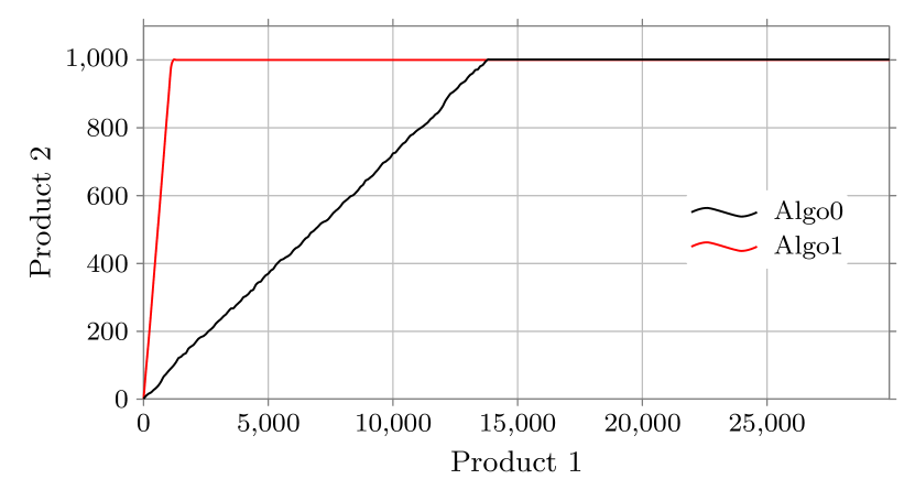
(a) Simulation of sales for Algorithms $0$ and $1$ run on separate inventories. Both algorithms sell all 1 000 attractive goods. Algorithm $0$ additionally sells $199\,528$ goods of type $1$, Algorithm $1$ sells $199\,325$. The differences between the two algorithms are within the fluctuations one expects. Surely, this simulation does not give rise to the conclusion that Algorithm $1$ outperforms Algorithm $0$. However, Algorithm $1$ sells the attractive goods earlier.

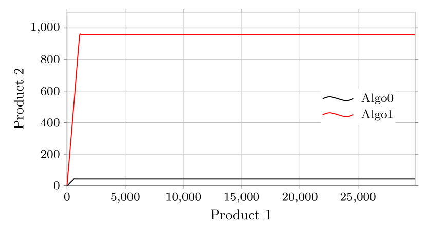
(b) Simulation of sales for Algorithms $0$ and $1$ run on shared inventory. Algorithm $0$ sells $99\,224$ items of good $1$ and $43$ items of good $2$, while Algorithm $1$ sells $99\,229$ items of product $1$ and the remaining $957$ items of product $2$. The huge difference in sales of the attractive good leads to a rejection of the null hypothesis (of both algorithms performing equally well) by the chi-squared test, the $p$-value in this simulation is $0.0369\ldots<0.05$.

Figure 3. Simulation of sales in Example 1.1 on separate and shared inventory.

It is a common approach to test for the higher probability of a sale by assuming an independent sample and using a $G$-test or the asymptotically equivalent two-sample chi-squared test. The hypothesis is that the conversion rates are identical in both samples. For simplicity, in the paper at hand, we shall always consider the chi-squared test. The test statistics for the latter is

$$\chi^{2}=\sum_{i=0,1}\frac{(\ell_{i}-\ell\frac{n_{i}}{n})^{2}}{\ell\frac{n_{i}}{n}}+\sum_{i=0,1}\frac{(n_{i}\!-\!\ell_{i}-\ell\frac{n_{i}}{n})^{2}}{(n-\ell)\frac{n_{i}}{n}}.$$

The hypothesis is rejected if $\chi^{2}>q_{1-\alpha}$ where $\alpha\in(0,1)$ is the significance level and $q_{1-\alpha}$ is the $(1\!-\!\alpha)$-quantile of the chi-squared distribution with one degree of freedom, see [3, Chapter 17].

Throughout the paper, we shall return repeatedly to Example 1.1 and discuss it in the light of our findings.

We shall discuss a variant of this example later on showing that ignoring the dependencies might also lead to too high false negative rates, see Example 3.8 below.

2. Model assumptions

We return to the general situation, in which a website offers two types of goods, good $1$ and good $2$. During a test phase, in which a new website design is used in parallel, the website has $n$ visitors. Suppose that the website has a practically unlimited supply of items of good $1$, while there are only $c_{n}\in\{1,2,3,\ldots\}=\vcentcolon\mathbb{N}$ items of good $2$. Typically, $n$ will be very large and $c_{n}$ will also be large, but significantly smaller than $n$. Whenever a user visits the website, a coin with success probability $p$ is tossed. If the coin shows heads, the new website design is displayed, whereas if the coin shows tails, the old design is displayed. We thus observe a sample $((x_{1},y_{1},i_{1}),\ldots,(x_{n},y_{n},i_{n}))\in(\mathbb{N}_{0}^{2}\times\{0,1\})^{n}$ where $\mathbb{N}_{0}\vcentcolon=\mathbb{N}\cup\{0\}$. Here, $x_{k}$ and $y_{k}$ are the numbers of goods of type $1$ and $2$, respectively, that have been bought by the $k^{\rm th}$ visitor of the website during the test phase, while $i_{k}=1$ if the new design has been displayed to the $k^{\rm th}$ visitor, and $i_{k}=0$, otherwise. We consider $((x_{1},y_{1},i_{1}),\ldots,(x_{n},y_{n},i_{n}))$ as the realization of a random vector $((X_{1},Y_{1},I_{1}),\ldots,(X_{n},Y_{n},I_{n}))$. We define $Z_{k}\vcentcolon=\mathbbm{1}_{\{X_{k}+Y_{k}>0\}}$ to be the indicator of the event that the $k^{\rm th}$ customer bought something. Further, we set $\mathbf{r}_{k}\vcentcolon=(s_{k},t_{k})\vcentcolon=(x_{1},y_{1})+\ldots+(x_{k},y_{k})$ and $\mathbf{R}_{k}\vcentcolon=(S_{k},T_{k})\vcentcolon=(X_{1},Y_{1})+\ldots+(X_{k},Y_{k})$ for $k=0,\ldots,n$ where the empty sum is defined to be the zero vector.

2.1. The classical model assuming independence

Many website owners in e-commerce use the $G$-test or the chi-squared test in the given situation. This test only uses the information whether or not a good was purchased, that is, the only information from the sample $((X_{1},Y_{1},I_{1}),\ldots,(X_{n},Y_{n},I_{n}))$ used by the test is $(Z_{1},I_{1}),\ldots,(Z_{n},I_{n})$. This amounts to the following model assumptions.

• There is a sequence $(I_{1},I_{2},\ldots)$ of i.i.d. copies of a Bernoulli variable $I$ with $\mathbb{P}(I=1)=p=1-\mathbb{P}(I=0)\in(0,1)$.

• There are a random variable $\zeta$ and $p_{0},p_{1}\in(0,1)$ such that

  $$\mathbb{P}(Z_{k}\in\cdot|I_{k}=i)=\mathbb{P}(\zeta\in\cdot|I=i)=\mathrm{Ber}(p_{i})(\cdot)=p_{i}\delta_{1}(\cdot)+(1-p_{i})\delta_{0}(\cdot)$$

  for all $k\in\mathbb{N}$ and $i=0,1$,

• The family $((I_{k},Z_{k}))_{k\in\mathbb{N}}$ is independent.

Here, and throughout the paper, for $x\in\mathbb{R}^{d}$, we write $\delta_{x}$ for the Dirac measure with a point at $x$. Assumptions ($\chi 1$) through ($\chi 3$) possess the following interpretations.

($\chi 1$): The random variable $I_{k}$ models the coin toss that is used to decide whether the new or the old website design is displayed to the $k^{\rm th}$ visitor of the website during the test phase.

($\chi 2$): The random variable $Z_{k}$ is the indicator of the event that the $k^{\rm th}$ visitor bought something.

($\chi 3$): The independence assumption in the context of the low inventory problem is made for simplicity. We question the feasibility of this assumption in the present paper.

2.2. A model incorporating low inventory of a popular good.

We propose a simple model in which we keep track of the inventory of a rare good. Throughout the paper, we shall refer to this model as the ‘model incorporating low inventory’. By $c_{n}\in\mathbb{N}$ we denote the quantity at which the rare good is available. The most important case we consider is where $c_{n}$ is asymptotically equivalent to a constant times $\sqrt{n}$. However, as we need this assumption only occasionally, throughout the paper, we only assume that $(c_{n})_{n\in\mathbb{N}}$ is a non-decreasing unbounded sequence of integers which is regularly varying with index $\rho\in(0,1]$ at infinity, that is,

$$\lim_{n\to\infty}\frac{c_{\lfloor nt\rfloor}}{c_{n}}=t^{\rho},\quad t\geq 0$$ (2.1)

and further $c_{n}=O(n)$ as $n\to\infty$, which is relevant only if $\rho=1$. Notice that the case $c_{n}\sim\mathrm{const}\cdot\sqrt{n}$ is covered. Indeed, in this case, we have $\rho=\frac{1}{2}$.

In the next step, we informally describe the evolution of the process $(\mathbf{R}_{k})_{k\in\mathbb{N}_{0}}$. Let $C_{n}\vcentcolon=\mathbb{N}_{0}\times([0,c_{n}]\cap\mathbb{N}_{0})$, $C_{n}^{\circ}\vcentcolon=\mathbb{N}_{0}\times([0,c_{n})\cap\mathbb{N}_{0})$ and $\partial C_{n}\vcentcolon=C_{n}\setminus C_{n}^{\circ}=\mathbb{N}\times\{c_{n}\}$. At each step, a coin with success probability $p$ is tossed. Depending on whether the coin shows heads or tails, the walk attempts to make one step according to a probability distribution $\mu_{1}$ or $\mu_{0}$, respectively, on $\mathbb{N}_{0}^{2}$. The step is actually performed if the walk stays in the strip $C_{n}$. Otherwise, another independent coin with success probability $q$ is tossed. If the second coin shows heads, the walk moves in each coordinate direction according to the attempted step as far as possible but stops at the boundary of $C_{n}$. If the second coin shows tails, the walk stays put. Once the walk is on the boundary of $C_{n}$, it moves there according to a one-dimensional random walk in horizontal direction.

Figure 4. The $2$-dimensional random walk in a semi-infinite strip. The $k^{\rm th}$ step is drawn in red if $I_{k}=1$ and it is drawn in blue, otherwise. The walk moves in the strip until it hits the upper boundary and continues on the boundary as a $1$-dimensional random walk. Here, we use the particular model from Example 1.1. Notice that the majority of steps have length zero and are not displayed.

The underlying model assumptions are the following.

• There are two sequences $(I_{1},I_{2},\ldots)$ and $(J_{1},J_{2},\ldots)$ of i.i.d. copies of Bernoulli variables $I$ and $J$, respectively, with $\mathbb{P}(I=1)=p=1-\mathbb{P}(I=0)\in(0,1)$ and $\mathbb{P}(J=1)=q=1-\mathbb{P}(J=0)\in[0,1]$.

• There are a sequence $(\xi_{1},\eta_{1}),(\xi_{2},\eta_{2}),\ldots$ of i.i.d. copies of a random variable $(\xi,\eta)$ and two probability measures $\mu_{0}$, $\mu_{1}$ on $\mathbb{N}_{0}^{2}$ satisfying $\mu_{i}(\{(a,b)\})>0$ for all $(a,b)\in\{0,1\}^{2}$ and $i=0,1$ such that

  $$\mathbb{P}((\xi_{k},\eta_{k})\in\cdot|I_{k}=i)=\mathbb{P}((\xi,\eta)\in\cdot|I=i)=\mu_{i}(\cdot)$$

  for all $k\in\mathbb{N}$ and $i=0,1$. We set $\mu_{p}(\cdot)\vcentcolon=p\mu_{1}(\cdot)+(1-p)\mu_{0}(\cdot)=\mathbb{P}((\xi,\eta)\in\cdot)$.

• There are a probability measure $\nu$ on $\mathbb{N}_{0}$ and i.i.d. copies $\theta_{1},\theta_{2},\ldots$ of a random variable $\theta$ with $\mathbb{P}(\theta\in\cdot)=\nu(\cdot)$.

• The sequences $(I_{k})_{k\in\mathbb{N}}$, $(J_{k})_{k\in\mathbb{N}}$, $((\xi_{k},\eta_{k}))_{k\in\mathbb{N}}$ and $(\theta_{k})_{k\in\mathbb{N}}$ are independent; all random variables have finite second moments.

• Let $k\in\mathbb{N}$. If $\mathbf{R}_{k-1}=(S_{k-1},T_{k-1})\in C_{n}^{\circ}$, then

  $$\mathbf{R}_{k}=\begin{cases}\mathbf{R}_{k-1}+(\xi_{k},\eta_{k})&\text{if }T_{k-1}+\eta_{k}\leq c_{n},\\ (S_{k},(T_{k-1}+\eta_{k})\wedge c_{n})&\text{if }T_{k-1}+\eta_{k}>c_{n}\text{ and }J_{k}=1,\\ \mathbf{R}_{k-1}&\text{if }T_{k-1}+\eta_{k}>c_{n}\text{ and }J_{k}=0.\end{cases}$$

  On the other hand, if $\mathbf{R}_{k-1}\in\partial C_{n}$, then $T_{k-1}=c_{n}$. In this case,

  $$\mathbf{R}_{k}=\mathbf{R}_{k-1}+(\theta_{k},0).$$

  Finally, define $(X_{k},Y_{k})\vcentcolon=\mathbf{R}_{k}-\mathbf{R}_{k-1}$.

The interpretations of these assumptions are the following.

(A1): The random variable $I_{k}$ models the coin toss that is used to decide whether the new or the old website design is displayed to the $k^{\rm th}$ visitor of the website during the test phase. The random variable $J_{k}$ models the preference of the $k^{\rm th}$ visitor. If $J_{k}=1$, then the user must buy. Users with $J_{k}=0$ only buy when they get exactly what they want in the first place.

(A2): The random variable $(\xi_{k},\eta_{k})$ can be interpreted as the vector of goods that the $k^{\rm th}$ visitor would buy when visiting the (displayed version of the) website if there was enough supply of these goods.

(A3): The random variable $\theta_{k}$ can be interpreted as the amount of type-$1$ goods that the $k^{\rm th}$ visitor would buy when visiting the website and finding only goods of type $1$ left.

(A4): This is an independence assumption which is made to keep the model as simple as possible.

(A5): The random variable $(X_{k},Y_{k})$ models what is actually bought by the $k^{\rm th}$ user. This depends on the needs of the user, $\xi_{k}$, $\eta_{k}$ and $\theta_{k}$, the remaining amount of the rare good $2$ given by $c_{n}-T_{k-1}$, and the user’s preference $J_{k}$. If there are enough goods available to meet the needs of the $k^{\rm th}$ user, then the user will buy exactly the needed amounts, namely, $\xi_{k}$ of good $1$ and $\eta_{k}$ of good $2$. If good $2$ is not available at a sufficient quantity, then the user will either buy as much as possible of each of the goods if $J_{k}=1$ or nothing at all if $J_{k}=0$. If there is nothing left of good $2$, the user will buy $\theta_{k}$ of good $1$.

Notice that in both models, $\mathbb{P}$ depends on $p$, which is not explicit in the notation. While in large parts of the paper, $p$ is fixed, in some places, however, it is important to make the dependence of $\mathbb{P}$ on $p$ explicit. In these places, we write $\mathbb{P}_{p}$. Often, this will be $\mathbb{P}_{0}$ or $\mathbb{P}_{1}$, which correspond to the situations where only one version of the website is used.

Let us introduce some notation for various characteristics of the above variables which we shall use throughout the paper.

• We set ${\bf m}_{0}\vcentcolon=(m^{\xi}_{0},m^{\eta}_{0})\vcentcolon=\mathbb{E}[(\xi,\eta)|I=0]$, ${\bf m}_{1}\vcentcolon=(m^{\xi}_{1},m^{\eta}_{1})\vcentcolon=\mathbb{E}[(\xi,\eta)|I=1]$ and ${\bf m}\vcentcolon=(m^{\xi},m^{\eta})\vcentcolon=\mathbb{E}[(\xi,\eta)]=p{\bf m}_{1}+(1-p){\bf m}_{0}$. Notice that $m^{\xi}$ and $m^{\eta}$ depend on $p$ even though this is not explicit in the notation.

• The covariance matrices of the probability measures $\mu_{i}$, $i=0,1$ are denoted by ${\bf C}_{i}$, $i=0,1$, respectively. The covariance matrix of the probability measure $\mu_{p}$ is then

  $${\bf C}=p{\bf C}_{1}+(1-p){\bf C}_{0}=\left(\begin{matrix}\sigma_{\xi}^{2}&\rho_{\xi\eta}\\ \rho_{\xi\eta}&\sigma^{2}_{\eta}\end{matrix}\right).$$

• We denote by $m^{\theta}=\mathbb{E}[\theta]$ and $\sigma^{2}_{\theta}=\mathrm{Var}[\theta]$, the mean and the variance of the probability measure $\nu$.

• Finally, we set $p_{i}\vcentcolon=\mu_{i}(\{(0,0)^{\mathsf{c}}\})=\mathbb{P}(\xi+\eta>0|I=i)$ for $i=0,1$ and $p_{\theta}\vcentcolon=\mathbb{P}(\theta>0)$. The $p_{i}$, $i=0,1$ and $p_{\theta}$ are the theoretical conversion rates.

Example 2.1 (Ranking experiment, take 2).

We return to Example 1.1 and briefly explain how this example fits into the framework of the above model. The number of visitors during the test phase is $n=4\cdot 10^{6}$. The quantity of the attractive good $2$ is $c_{n}=1\,000=\frac{1}{2}\cdot\sqrt{n}$. Website visitors view each version of the website with equal probability, so $I_{1},I_{2},\ldots$ have success probability $p=\frac{1}{2}$.

Further, as can be readily seen from Figure 1,

$$\textstyle\mu_{0}=\frac{96}{100}(\frac{1}{20}\delta_{(1,0)}+\frac{19}{20}\delta_{(0,0)})+\frac{4}{100}(\frac{1}{10}\delta_{(0,1)}+\frac{9}{10}\delta_{(0,0)})=\frac{948}{1\,000}\delta_{(0,0)}+\frac{4}{1\,000}\delta_{(0,1)}+\frac{48}{1\,000}\delta_{(1,0)}.$$

Analogously, from Figure 2, we deduce

$$\textstyle\mu_{1}=\frac{1}{5}(\frac{1}{20}\delta_{(1,0)}+\frac{19}{20}\delta_{(0,0)})+\frac{4}{5}(\frac{1}{10}\delta_{(0,1)}+\frac{9}{10}\delta_{(0,0)})=\frac{91}{100}\delta_{(0,0)}+\frac{8}{100}\delta_{(0,1)}+\frac{1}{100}\delta_{(1,0)}.$$

Moreover, the law of $\theta$ is given by $\frac{19}{20}\delta_{(0,0)}+\frac{1}{20}\delta_{(1,0)}$. The variables $J_{k}$ are irrelevant in the given situation as step sizes here are at most one, hence there will never be the situation where a visitor attempts to buy more of the popular good than what is left. We conclude that the theoretical conversion rates are given by

$$\textstyle p_{0}=\mu_{0}(\{(0,0)\}^{\mathsf{c}})=\frac{52}{1\,000},\quad p_{1}=\mu_{1}(\{(0,0)\}^{\mathsf{c}})=\frac{9}{100}\quad\text{and}\quad p_{\theta}=\frac{5}{100}.$$

We shall see that if $c_{n}=c\sqrt{n}$, then the chi-squared test will reject the hypothesis with probability tending to $1$ as $c$ becomes large. On the other hand, we shall demonstrate that Algorithm $2$ does not perform better given the model assumptions (A1) through (A5).

3. Testing for the higher conversion rate

We address the question which algorithm, when used alone, leads to the higher conversion rate, where the conversion rate is the total number of sales divided by the total number of visitors. More formally, for $i=0,1$, we define

$$N_{n}^{(i)}\vcentcolon=\sum_{k=1}^{n}\mathbbm{1}_{\{I_{k}=i\}}\quad\text{and}\quad L_{n}^{(i)}\vcentcolon=\sum_{k=1}^{n}\mathbbm{1}_{\{Z_{k}>0,\,I_{k}=i\}},$$

which model the number of visitors of website version $i$ and the number of those visitors who make a purchase. We set $L_{n}\vcentcolon=L_{n}^{(0)}+L_{n}^{(1)}$, which is the total number of purchases, and notice that $N_{n}^{(0)}+N_{n}^{(1)}=n$. Then

$$C_{n}^{(i)}\vcentcolon=\tfrac{L_{n}^{(i)}}{N_{n}^{(i)}}$$

is the empirical conversion rate in group $i$. We stipulate that $C_{n}^{(i)}\vcentcolon=0$ on $\{N_{n}^{(i)}=0\}$.

If one chooses $p\in\{0,1\}$, then $C_{n}^{(p)}$ under $\mathbb{P}_{p}$ is the empirical conversion rate when only website $i=p$ is used. In view of this, version $1$ of the website is better than version $0$ if $C_{n}^{(1)}$ under $\mathbb{P}_{1}$ is ‘larger’ than $C_{n}^{(0)}$ under $\mathbb{P}_{0}$. Here, the term ‘larger’ is not specified a priori, so we need to clarify what we mean by this.

3.1. The chi-squared test statistics in the classical model

In the classical model, i.e., if assumptions ($\chi 1$), ($\chi 2$) and ($\chi 3$) are in force, $Z_{1},Z_{2},\ldots$ are i.i.d. with expectation $\mathbb{E}[Z_{1}]=\mathbb{P}(Z_{1}=1)=pp_{1}+(1-p)p_{0}$. Hence, by the strong law of large numbers, for $p\in\{0,1\}$,

$$c^{(p)}\vcentcolon=\lim_{n\to\infty}C_{n}^{(p)}=\lim_{n\to\infty}\tfrac{1}{n}L_{n}^{(p)}=\mathbb{P}(\xi+\eta>0)=pp_{1}+(1-p)p_{0}\quad\text{a.\,s.}$$

Consequently, testing whether $C_{n}^{(1)}$ under $\mathbb{P}_{1}$ is ‘different’ from $C_{n}^{(0)}$ under $\mathbb{P}_{0}$ can be formulated as follows:

$$H_{0}:p_{1}=p_{0}\qquad\text{vs.}\qquad H_{1}:p_{1}\not=p_{0}.$$

More interest, in fact, would be in the corresponding one-sided test problem. Hence, in this case, it is a classical test problem and widely used tests for this problem are the chi-squared test, the $G$-test, and Fisher’s exact test. To keep the paper short, we shall always restrict attention to the chi-squared test. For the reader’s convenience, we recall some facts about this test.

Table 1. Contingency table

	purchase	no purchase	$\sum$
group 0	$L_{n}^{(0)}$	$N_{n}^{(0)}-L_{n}^{(0)}$	$N_{n}^{(0)}$
group 1	$L_{n}^{(1)}$	$N_{n}^{(1)}-L_{n}^{(1)}$	$N_{n}^{(1)}$
$\sum$	$L_{n}$	$n-L_{n}$	$n$

The test statistics for the chi-squared test is

$$\chi^{2}\vcentcolon=\sum_{i=0,1}\frac{\big{(}L_{n}^{(i)}-L_{n}\frac{N_{n}^{(i)}}{n}\big{)}^{2}}{L_{n}\frac{N_{n}^{(i)}}{n}}+\sum_{i=0,1}\frac{\big{(}N_{n}^{(i)}\!-\!L_{n}^{(i)}-(n\!-\!L_{n})\frac{N_{n}^{(i)}}{n}\big{)}^{2}}{(n\!-\!L_{n})\frac{N_{n}^{(i)}}{n}}.$$ (3.1)

If ($\chi$1) through ($\chi 3$) are in force, as $n\to\infty$, the distribution of $\chi^{2}$ approaches a chi-squared distribution with $1$ degree of freedom [3, Chapter 17]. Write $q_{1-\alpha}$ for the $1-\alpha$ quantile of the chi-squared distribution with $1$ degree of freedom. Then, with significance level of $\alpha$, the hypothesis is rejected if $\chi^{2}>q_{1-\alpha}$.

3.2. The limiting law of the chi-squared test statistics in the model incorporating low inventory

Now suppose that there is a rare but popular good, i.e., suppose that the model assumptions (A1) through (A5) hold. One goal of this paper is to point out in a quantitative way that when (A1) through (A5) instead of ($\chi 1$) through ($\chi 3$) are in force, then the chi-squared test may produce too many false positives. In other words, it may fail to hold the specified significance level. This is because the distribution of $\chi^{2}$ under the null hypothesis is different when (A1) through (A5) rather than ($\chi 1$) through ($\chi 3$) are in force. The detailed statement is given in the following theorem.

Theorem 3.1.

Suppose that (A1) through (A5) and (2.1) are in force. Assume additionally that

$$d_{\infty}\vcentcolon=\lim_{n\to\infty}\frac{c_{n}}{\sqrt{n}}\in[0,\infty).$$

Then the chi-squared statistics defined by (3.1) satisfies

$$\textstyle\chi^{2} \mathrel{\vbox{\offinterlineskip\halign{\hfil#\hfil\cr$\scriptscriptstyle\mathrm{d}$\cr\kern 0.6458pt\cr$\to$\cr}}}\left(\mathcal{N}-\frac{d_{\infty}(p_{0}-p_{1})\sqrt{p(1-p)}}{m^{\eta}\sqrt{p_{\theta}(1-p_{\theta})}}\right)^{\!\!2}\qquad\text{as }n\to\infty$$

where $\mathcal{N}$ is a standard normal random variable.

Hence, if one applies the chi-squared test with significance level $\alpha\in(0,1)$ in the given situation, the test rejects the hypothesis with (asymptotic) probability

$$\textstyle\mathbb{P}\left(\left(\mathcal{N}-\frac{d_{\infty}(p_{0}-p_{1})\sqrt{p(1-p)}}{m^{\eta}\sqrt{p_{\theta}(1-p_{\theta})}}\right)^{\!\!2}>q_{1-\alpha}\right)>\mathbb{P}\left(\mathcal{N}^{2}>q_{1-\alpha}\right)=\alpha.$$

In fact, the probability on the left-hand side tends to $1$ as $d_{\infty}\to\infty$. We specialize to the situation of Example 1.1.

Example 3.2 (Ranking experiment, take 3).

Recall the situation of Example 1.1. Then, see also Example 2.1, we have

$$\textstyle p=\frac{1}{2},\qquad p_{\theta}=\frac{1}{20},\qquad p_{0}=\frac{52}{1\,000},\qquad p_{1}=\frac{9}{100},\qquad m^{\eta}=\frac{42}{1\,000}\qquad\text{and}\qquad d_{\infty}=\frac{1}{2}.$$

Consequently,

$$\frac{d_{\infty}(p_{0}-p_{1})\sqrt{p(1-p)}}{m^{\eta}\sqrt{p_{\theta}(1-p_{\theta})}}=\frac{\frac{1}{2}\cdot\frac{-38}{1\,000}\cdot\frac{1}{2}}{\frac{42}{1\,000}\cdot\sqrt{\frac{19}{400}}}=-\frac{\sqrt{19}\cdot 5}{21}=-1.037833\ldots$$ (3.2)

Hence, in the given situation, the chi-squared test rejects the hypothesis with (asymptotic) probability

$$\textstyle\mathbb{P}\left((\mathcal{N}+1.037833)^{2}>q_{95\%}\right)=0.1795898\ldots>0.05.$$

This becomes worse as $d_{\infty}$ becomes larger, see Figure 5 below.

Figure 5. False-positive probability as a function of $d_{\infty}$ with all other parameters fixed as in (3.2).

At first glance, this may occur to be no problem as $p_{1}>p_{0}$, so one is tempted to guess that algorithm $1$ performs better than algorithm $0$ and what we see above is just the power of the test, which becomes better as $d_{\infty}$ becomes large. However, we shall argue in Example 3.6 below that the two algorithms perform equally well when used separately.

Next, we show that in the general situation, assuming that (A1) through (A5) hold and that $\frac{c_{n}}{n}\to 0$, we show that on the linear scale, the asymptotic empirical conversion rates of the two versions of the website, when used separately, are identical.

Theorem 3.3.

Suppose that (A1) through (A5) hold and that $c_{\infty}\vcentcolon=\lim_{n\to\infty}\frac{c_{n}}{n}=0$. Then, for $p\in\{0,1\}$,

$$\lim_{n\to\infty}C_{n}^{(p)}=p_{\theta}\quad\mathbb{P}_{p}\text{-a.\,s.}$$

Proof.

The result is a consequence of Theorem 3.4 below. ∎

Hence, in the relevant regime ($\frac{c_{n}}{n}\to 0$) the first order of growth of $C_{n}^{(p)}$ depends only on what happens after the popular good is sold out. According to our model assumptions, the two versions of the website have identical performance once the popular good is sold out. This implies that on the linear scale, there is no difference between the two versions of the website. Hence, we need to make a comparison on a finer scale.

3.3. A joint limit theorem for the group sizes and numbers of purchases in each group

As $\chi^{2}$ is a function of $(N_{n}^{(0)},N_{n}^{(1)},L_{n}^{(0)},L_{n}^{(1)})$, a limit theorem for $\chi^{2}$ follows from one for the above vector via the continuous mapping theorem [1, Theorem 2.7]. We begin with a strong law of large numbers for the variables $L_{n}^{(0)}$ and $L_{n}^{(1)}$ (the corresponding result for $N_{n}^{(0)}$ and $N_{n}^{(1)}$ is classical).

Theorem 3.4.

Suppose that (A1) through (A5) are in force and that the limit

$$c_{\infty}\vcentcolon=\lim_{n\to\infty}\frac{c_{n}}{n}\in[0,\infty)$$

exists. If $c_{\infty}\in[0,\frac{1}{m^{\eta}})$, then

$$\tfrac{1}{n}L_{n}^{(0)}\to(1-p)p_{\theta}+c_{\infty}(1-p)\tfrac{1}{m^{\eta}}(p_{0}-p_{\theta})\quad\text{and}\quad\tfrac{1}{n}L_{n}^{(1)}\to pp_{\theta}+c_{\infty}p\tfrac{1}{m^{\eta}}(p_{1}-p_{\theta})\quad\text{a.\,s.}$$

In particular, in the most relevant case $c_{\infty}=0$,

$$\tfrac{1}{n}L_{n}^{(0)}\to(1-p)p_{\theta}\quad\text{and}\quad\tfrac{1}{n}L_{n}^{(1)}\to pp_{\theta}\quad\text{a.\,s.}$$

If $c_{\infty}>\frac{1}{m^{\eta}}$, then

$$\tfrac{1}{n}L_{n}^{(0)}\to(1-p)p_{0}\quad\text{and}\quad\tfrac{1}{n}L_{n}^{(1)}\to pp_{1}\quad\text{a.\,s.}$$

We continue with the asymptotic law of the vector $(N_{n}^{(0)},N_{n}^{(1)},L_{n}^{(0)},L_{n}^{(1)})$, suitably shifted and scaled in the most relevant scenario where $c_{n}$ is of the order $\sqrt{n}$.

Theorem 3.5.

Suppose that (A1) through (A5) are in force and suppose in addition to (2.1) that the limit

$$d_{\infty}=\lim_{n\to\infty}\frac{c_{n}}{\sqrt{n}}\in[0,\infty)$$

exists, we have, as $n\to\infty$,

$$\bigg{(}\frac{N^{(0)}_{n}-(1-p)n}{\sqrt{n}},\frac{N^{(1)}_{n}-pn}{\sqrt{n}},\frac{L_{n}^{(0)}-n(1-p)p_{\theta}}{\sqrt{n}},\frac{L_{n}^{(1)}-npp_{\theta}}{\sqrt{n}}\bigg{)}\\ \mathrel{\vbox{\offinterlineskip\halign{\hfil#\hfil\cr$\scriptscriptstyle\mathrm{d}$\cr\kern 0.6458pt\cr$\to$\cr}}}d_{\infty}\big{(}0,0,(1\!-\!p)\tfrac{1}{m^{\eta}}(p_{0}\!-\!p_{\theta}),p\tfrac{1}{m^{\eta}}(p_{1}\!-\!p_{\theta})\big{)}+(G_{1},-G_{1},G_{2},G_{3})$$ (3.3)

where $\left(G_{1},G_{2},G_{3}\right)$ is a centered Gaussian vector with covariance matrix

$$\mathbf{V_{1}}=\left(\begin{matrix}p(1\!-\!p)&p(1\!-\!p)p_{\theta}&-p(1\!-\!p)p_{\theta}\\ p(1\!-\!p)p_{\theta}&p_{\theta}(1\!-\!p)(1\!-\!p_{\theta}(1\!-\!p))&-p(1\!-\!p)p_{\theta}^{2}\\ -p(1\!-\!p)p_{\theta}&-p(1\!-\!p)p_{\theta}^{2}&pp_{\theta}(1\!-\!pp_{\theta})\\ \end{matrix}\right).$$ (3.4)

Notice that the theorem contains a limit theorem for the pure conversion rates $C_{n}^{(0)}$ and $C_{n}^{(1)}$ by choosing $p=0$ and projecting on the third coordinate or by choosing $p=1$ and projecting on the fourth component, respectively. This gives, with $\mathcal{N}(\mu,\sigma^{2})$ denoting a normal random variable with mean $\mu$ and variance $\sigma^{2}$,

$$\frac{L_{n}^{(0)}-np_{\theta}}{\sqrt{n}} \mathrel{\vbox{\offinterlineskip\halign{\hfil#\hfil\cr$\scriptscriptstyle\mathrm{d}$\cr\kern 0.6458pt\cr$\to$\cr}}}\mathcal{N}(d_{\infty}\tfrac{p_{0}\!-\!p_{\theta}}{m_{0}^{\eta}},p_{\theta}(1\!-\!p_{\theta}))\quad\text{under }\mathbb{P}_{0}$$ (3.7)

$$\text{and}\qquad\frac{L_{n}^{(1)}-np_{\theta}}{\sqrt{n}} \mathrel{\vbox{\offinterlineskip\halign{\hfil#\hfil\cr$\scriptscriptstyle\mathrm{d}$\cr\kern 0.6458pt\cr$\to$\cr}}}\mathcal{N}(d_{\infty}\tfrac{p_{1}\!-\!p_{\theta}}{m_{1}^{\eta}},p_{\theta}(1\!-\!p_{\theta}))\quad\text{under }\mathbb{P}_{1}$$ (3.10)

where $m^{\eta}=pm^{\eta}_{1}+(1-p)m^{\eta}_{0}$ with $p=0$ and $p=1$, respectively, has been used. Hence, if the two expectations in (3.7) and (3.10) coincide, then the performances of the two websites coincide asymptotically both on the linear scale as well as on the level of fluctuations. The subsequent example demonstrates that this can be the case even if $p_{0}\not=p_{1}$.

Example 3.6 (Ranking experiment, take 4).

Recall the situation of Example 1.1 and the calculations of Example 3.2:

$$\textstyle p_{\theta}=\frac{1}{20},\qquad p_{0}=\frac{52}{1\,000},\qquad p_{1}=\frac{9}{100},\qquad m_{0}^{\eta}=\frac{4}{1\,000},\qquad m_{1}^{\eta}=\frac{8}{100}\qquad\text{and}\qquad d_{\infty}=\frac{1}{2}.$$

Consequently,

$$\tfrac{p_{0}\!-\!p_{\theta}}{m_{0}^{\eta}}=\frac{\frac{2}{1\,000}}{\frac{4}{1\,000}}=\frac{1}{2}=\frac{\frac{4}{100}}{\frac{8}{100}}=\tfrac{p_{1}\!-\!p_{\theta}}{m_{1}^{\eta}}.$$

This means that the two limits in (3.7) and (3.10) coincide in the given example even though $p_{1}>p_{0}$.

From Theorem 3.5, we may immediately deduce a limit theorem for $\chi^{2}$, which is a preliminary version of Theorem 3.1.

Corollary 3.7.

Suppose that (A1) through (A5) and (2.1) are in force and that the limit

$$d_{\infty}=\lim_{n\to\infty}\frac{c_{n}}{\sqrt{n}}\in[0,\infty)$$

exists, we have the following limit theorem for the chi-squared statistics defined by (3.1)

$$\chi^{2} \mathrel{\vbox{\offinterlineskip\halign{\hfil#\hfil\cr$\scriptscriptstyle\mathrm{d}$\cr\kern 0.6458pt\cr$\to$\cr}}}\frac{(d_{2}+G_{2}-p_{\theta}G_{1}-(1-p)(d_{2}+d_{3}+G_{2}+G_{3}))^{2}}{(1-p_{\theta})p_{\theta}(1-p)}$$

$$\hphantom{\mathrel{\vbox{\offinterlineskip\halign{\hfil#\hfil\cr$\scriptscriptstyle\mathrm{d}$\cr\kern 0.6458pt\cr$\to$\cr}}}\ }+\frac{(d_{3}+G_{3}+p_{\theta}G_{1}-p(d_{2}+d_{3}+G_{2}+G_{3}))^{2}}{(1-p_{\theta})p_{\theta}p}\qquad\text{as }n\to\infty$$

where $(0,0,d_{2},d_{3})$ denotes the expectation of the right-hand side in (3.3) and $(G_{1},G_{2},G_{3})$ is the Gaussian vector from Theorem 3.5.

We close this section with another example showing that ignoring the dependencies might also lead to a high false negative rate.

Example 3.8 (Ranking experiment with picky customers).

We consider a variant of Example 1.1 in which there are picky customers that will only buy the rare good. This time, we use the former Algorithm $1$ from above as the default algorithm displaying the rare goods first. The former Algorithm $0$ strategically keeps the rare inventory for later arrival of picky customers by ranking the rare good low. In an experiment with shared inventory, Algorithm $1$ sells off the rare good greedily, and the value of Algorithm $0$’s strategy will not be properly assessed in the model ignoring dependencies. We make this precise in the following.

Again suppose that during a test phase, $n=4\,000\,000$ customers visit the website. Again, there are $c_{n}=1\,000$ rare goods while good $1$ is available at sufficient quantities.

The algorithms work as in Example 1.1, but there is a difference in the behavior of the customers. We assume that, independent of all other customers, each customer has a $1\%$ chance of being picky. If not picky, the customer behaves like the customers of Example 1.1. A picky customer, however, will search as long as required to check whether there is something of the rare good left. If the rare good is still available, the picky customer buys one unit with $50\%$ chance. Otherwise, the customer leaves the website. The overviews given in Figure 2 still apply to regular customers, for picky customers and when good 2 is still available, there is a simplified decision tree:

Figure 6. Ranking experiment: Picky customer behavior when good $2$ is still available

A calculation of the relevant model parameters in this example based on the corresponding parameter values from Example 3.2 gives $p=\frac{1}{2}$ and $d_{\infty}=\frac{1}{2}$ as before and

$$\textstyle p_{\theta}=\frac{99}{100}\cdot\frac{1}{20},\quad p_{0}=\frac{99}{100}\cdot\frac{52}{1\,000}+\frac{1}{100}\cdot\frac{1}{2},\quad p_{1}=\frac{99}{100}\cdot\frac{9}{100}+\frac{1}{100}\cdot\frac{1}{2},\quad m^{\eta}=\frac{99}{100}\cdot\frac{42}{1\,000}+\frac{1}{100}\cdot\frac{1}{2}.$$

We shall now show that Algorithm $0$ performs actually better than Algorithm $1$. We have

$$\textstyle m_{0}^{\eta}=\frac{99}{100}\cdot\frac{4}{1\,000}+\frac{1}{100}\cdot\frac{1}{2}\quad\text{and}\quad m_{1}^{\eta}=\frac{99}{100}\cdot\frac{8}{100}+\frac{1}{100}\cdot\frac{1}{2}.$$

Consequently,

$$d_{\infty}\cdot\tfrac{p_{0}\!-\!p_{\theta}}{m_{0}^{\eta}}=\frac{349}{896}>\frac{223}{842}=d_{\infty}\cdot\tfrac{p_{1}\!-\!p_{\theta}}{m_{1}^{\eta}}.$$

In view of (3.7) and (3.10), Algorithm $0$ does perform better than Algorithm $1$. Now let us calculate the probability that the chi-squared test rejects the hypothesis that Algorithm $0$ and Algorithm $1$ perform equally well. To this end, we first calculate

$$\frac{d_{\infty}(p_{1}-p_{0})\sqrt{p(1-p)}}{m^{\eta}\sqrt{p_{\theta}(1-p_{\theta})}}=0.930852\ldots.$$

According to Theorem 3.1, the chi-squared test (with significance level $5\%$) rejects the hypothesis with probability $0.1536348\dotsc$. However, it is a standard practice to say that Algorithm $0$ is significantly better than Algorithm $1$ only when $\chi^{2}>q_{1-\alpha}$ and $C_{n}^{(0)}>C_{n}^{(1)}$ (with $\alpha\in(0,1)$ being the significance level). So, asymptotically, the power of the test is $\lim_{n\to\infty}\mathbb{P}(C_{n}^{(0)}>C_{n}^{(1)},\chi^{2}>q_{1-\alpha})$. We shall now calculate this probability in the given situation with $d_{\infty}=1/2$ but also as a function of $d_{\infty}$ to point out that the probability becomes arbitrarily small as $d_{\infty}$ becomes large. We begin by reformulating the condition $C_{n}^{(0)}>C_{n}^{(1)}$. Recall that $C_{n}^{(i)}=L_{n}^{(i)}/N_{n}^{(i)}$ for $i=0,1$. Hence,

$$C_{n}^{(0)}>C_{n}^{(1)}\quad\text{iff}\quad L_{n}^{(0)}N_{n}^{(1)}-L_{n}^{(1)}N_{n}^{(0)}>0$$

$$\text{iff}\quad(L_{n}^{(0)}-\tfrac{np_{\theta}}{2})(N_{n}^{(1)}-\tfrac{n}{2})-(L_{n}^{(1)}-\tfrac{np_{\theta}}{2})(N_{n}^{(0)}-\tfrac{n}{2})+\tfrac{np_{\theta}}{2}(N_{n}^{(1)}-N_{n}^{(0)})+\tfrac{n}{2}(L_{n}^{(0)}-L_{n}^{(1)})>0$$

$$\text{iff}\quad\frac{2}{\sqrt{n}}\frac{L_{n}^{(0)}-np_{\theta}/2}{\sqrt{n}}\cdot\frac{N_{n}^{(1)}-n/2}{\sqrt{n}}-\frac{2}{\sqrt{n}}\frac{L_{n}^{(1)}-np_{\theta}/2}{\sqrt{n}}\cdot\frac{N_{n}^{(0)}-n/2}{\sqrt{n}}$$

$$\hphantom{\text{iff}}\quad-p_{\theta}\frac{N_{n}^{(0)}-n/2}{\sqrt{n}}+p_{\theta}\frac{N_{n}^{(1)}-n/2}{\sqrt{n}}+\frac{L_{n}^{(0)}-np_{\theta}/2}{\sqrt{n}}-\frac{L_{n}^{(1)}-np_{\theta}/2}{\sqrt{n}}>0.$$

By Theorem 3.5 and Slutsky’s theorem, the two terms in the penultimate line tend to $0$ in probability as $n\to\infty$. By Theorem 3.5, the other summands converge in distribution so that in the limit, the above inequality becomes

$$-2p_{\theta}G_{1}+d_{\infty}\tfrac{p_{0}\!-\!p_{\theta}}{2m^{\eta}}+G_{2}-d_{\infty}\tfrac{p_{1}\!-\!p_{\theta}}{2m^{\eta}}-G_{3}>0,$$

which can be simplified to

$$-2p_{\theta}G_{1}+G_{2}-G_{3}>d_{\infty}\tfrac{p_{1}\!-\!p_{0}}{2m^{\eta}}.$$

By Theorem 3.1, $\chi^{2}$ converges also in distribution. According to Corollary 3.7, we can express the condition $\chi^{2}>q_{1-\alpha}$ in the limit as $n\to\infty$ in the form

$$(d_{2}+G_{2}-p_{\theta}G_{1}-\tfrac{1}{2}(d_{2}+d_{3}+G_{2}+G_{3}))^{2}+(d_{3}+G_{3}+p_{\theta}G_{1}-\tfrac{1}{2}(d_{2}+d_{3}+G_{2}+G_{3}))^{2}$$

$$>\tfrac{1}{2}(1-p_{\theta})p_{\theta}q_{1-\alpha}$$ (3.11)

where $(0,0,d_{2},d_{3})$ is the expectation vector in (3.3), i.e., $(0,0,d_{2},d_{3})=d_{\infty}\big{(}0,0,\tfrac{p_{0}\!-\!p_{\theta}}{2m^{\eta}},\tfrac{p_{1}\!-\!p_{\theta}}{2m^{\eta}}\big{)}$. Since the convergence in Theorem 3.5 is jointly and since the law of $(G_{1},G_{2},G_{3})$ on $\mathbb{R}^{3}$ is absolutely continuous with respect to Lebesgue measure, the Portmanteau theorem implies that

$$\lim_{n\to\infty}\mathbb{P}(\chi^{2}>q_{1-\alpha},C_{n}^{(0)}>C_{n}^{(1)})=\mathbb{P}\big{(}\text{\eqref{eq:chi^2 > q_1-alpha in terms of Gs} holds and }-2p_{\theta}G_{1}+G_{2}-G_{3}>d_{\infty}\tfrac{p_{1}\!-\!p_{0}}{2m^{\eta}}\big{)}.$$

In the given situation (with $d_{\infty}=\frac{1}{2}$), we have used a Monte Carlo simulation (with $2\cdot 10^{6}$ iterations) to estimate the power of the test resulting in an estimate of $0.001933\ldots$ Further, it is already immediate that the power tends to $0$ as $d_{\infty}$ tends to $\infty$ since $p_{1}>p_{0}$. To get a better quantitative picture, we have performed Monte Carlo simulations for 200 equidistant values of $d_{\infty}$ between $0$ and $1$, each with $2\cdot 10^{6}$ iterations. The results of the Monte Carlo simulations are displayed in Figure 7.

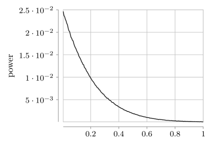
Figure 7. Monte Carlo simulation of the power of the test as a function of $d_{\infty}$ with all other parameters fixed as above.

In particular, for every value $d_{\infty}>0$, the estimate of the power of the test is strictly smaller than $0.025=\frac{\alpha}{2}$.

3.4. Functional limit theorem for the model incorporating low inventory

We deduce Theorem 3.5 from a more general result, namely, a joint functional central limit theorem. To formulate it, we need additional notation.

Henceforth, convergence in distribution of random elements in the Skorohod spaces $D([0,\infty),\mathbb{R}^{d})$ and $D((0,\infty),\mathbb{R}^{d})$ of $\mathbb{R}^{d}$-valued, right-continuous functions with existing left limits is with respect to the standard $J_{1}$-topology and will be denoted by $\Longrightarrow$. To distinguish between convergence in the above two spaces we adopt the following convention. The convergence is in $D([0,\infty),\mathbb{R}^{d})$ if the processes are written with subscript $(\cdot)_{t\geq 0}$, whilst if the subscript is $(\cdot)_{t>0}$, the convergence is in $D((0,\infty),\mathbb{R}^{d})$.

Let $({\bf B}(t))_{t\geq 0}=\left((B_{1}(t),\ldots,B_{7}(t))\right)_{t\geq 0}$ be a centered $7$-dimensional Brownian motion with covariance matrix

$$\mathbf{V}=\left(\begin{matrix}p_{0}(1\!-\!p)(1\!-\!p_{0}(1\!-\!p))&-p_{0}p_{1}p(1\!-\!p)&-p_{0}(1\!-\!p)p&(1\!-\!p)(m_{0}^{\xi}-m^{\xi}p_{0})\\ -p_{0}p_{1}p(1\!-\!p)&pp_{1}(1\!-\!pp_{1})&pp_{1}(1\!-\!p)&p(m_{1}^{\xi}-p_{1}m^{\xi})\\ -p_{0}(1\!-\!p)p&pp_{1}(1\!-\!p)&p(1\!-\!p)&p(m_{1}^{\xi}-m^{\xi})\\ (1\!-\!p)(m_{0}^{\xi}-m^{\xi}p_{0})&p(m_{1}^{\xi}-p_{1}m^{\xi})&p(m_{1}^{\xi}-m^{\xi})&\sigma^{2}_{\xi}\\ (1\!-\!p)(m_{0}^{\eta}-m^{\eta}p_{0})&p(m_{1}^{\eta}-p_{1}m^{\eta})&p(m_{1}^{\eta}-m^{\eta})&\rho_{\xi\eta}\\ p_{0}(1\!-\!p)pp_{\theta}&-p_{1}p(1\!-\!p)p_{\theta}&-p(1\!-\!p)p_{\theta}&(1\!-\!p)p_{\theta}(m_{0}^{\xi}-m^{\xi})\\ -p_{0}p(1\!-\!p)p_{\theta}&pp_{1}(1\!-\!p)p_{\theta}&p(1\!-\!p)p_{\theta}&pp_{\theta}(m_{1}^{\xi}-m^{\xi})\\ \end{matrix}\right.\\ \left.\begin{matrix}(1\!-\!p)(m_{0}^{\eta}-m^{\eta}p_{0})&p_{0}(1\!-\!p)pp_{\theta}&-p_{0}p(1\!-\!p)p_{\theta}\\ p(m_{1}^{\eta}-p_{1}m^{\eta})&-p_{1}p(1\!-\!p)p_{\theta}&pp_{1}(1\!-\!p)p_{\theta}\\ p(m_{1}^{\eta}-m^{\eta})&-p(1\!-\!p)p_{\theta}&p(1\!-\!p)p_{\theta}\\ \rho_{\xi\eta}&(1\!-\!p)p_{\theta}(m_{0}^{\xi}-m^{\xi})&pp_{\theta}(m_{1}^{\xi}-m^{\xi})\\ \sigma_{\eta}^{2}&(1\!-\!p)p_{\theta}(m_{0}^{\eta}-m^{\eta})&pp_{\theta}(m_{1}^{\eta}-m^{\eta})\\ (1\!-\!p)p_{\theta}(m_{0}^{\eta}-m^{\eta})&p_{\theta}(1\!-\!p)(1\!-\!p_{\theta}(1\!-\!p))&-p(1\!-\!p)p_{\theta}^{2}\\ pp_{\theta}(m_{1}^{\eta}-m^{\eta})&-p(1\!-\!p)p_{\theta}^{2}&pp_{\theta}(1\!-\!pp_{\theta})\\ \end{matrix}\right),$$ (3.12)

that is, ${\bf B}(t)={\bf V}^{1/2}{\bf B}^{\prime}(t)$, $t\geq 0$ where ${\bf B}^{\prime}(t)$ is a $7$-dimensional Brownian motion with independent components each being a one-dimensional standard Brownian motion, and ${\bf V}^{1/2}$ is the square root of the positive semi-definite matrix ${\bf V}$.

Theorem 3.9.

Suppose that (A1) through (A5) and (2.1) are in force and that the limit

$$c_{\infty}=\lim_{n\to\infty}\frac{c_{n}}{n}\in[0,\infty)$$

exists. If $c_{\infty}\in[0,\frac{1}{m^{\eta}})$, then, as $n\to\infty$,

$$\Bigg{(}\frac{N^{(0)}_{\lfloor nt\rfloor}-(1-p)nt}{\sqrt{n}},\frac{N^{(1)}_{\lfloor nt\rfloor}-pnt}{\sqrt{n}},\frac{L_{\lfloor nt\rfloor}^{(0)}-(1-p)\tfrac{1}{m^{\eta}}(p_{0}-p_{\theta})c_{\lfloor nt\rfloor}-nt(1-p)p_{\theta}}{\sqrt{n}},$$

$$\hphantom{\Bigg{(}\frac{N^{(0)}_{\lfloor nt\rfloor}-(1-p)nt}{\sqrt{n}},}\frac{L_{\lfloor nt\rfloor}^{(1)}-p\tfrac{1}{m^{\eta}}(p_{1}-p_{\theta})c_{\lfloor nt\rfloor}-ntpp_{\theta}}{\sqrt{n}}\Bigg{)}_{t>0}$$

$$\Longrightarrow\Big{(}-B_{3}(t),B_{3}(t),c_{\infty}^{\frac{1}{2}}\big{(}B_{1}\big{(}\tfrac{t}{m^{\eta}}\big{)}+(1\!-\!p)(p_{\theta}-p_{0})(m^{\eta})^{\frac{3}{2}}B_{5}(t)-B_{6}\big{(}\tfrac{t}{m^{\eta}}\big{)}\big{)}+B_{6}(t),$$

$$\hphantom{\Longrightarrow\big{(}-B_{3}(t),B_{3}(t),}c_{\infty}^{\frac{1}{2}}\big{(}B_{2}\big{(}\tfrac{t}{m^{\eta}}\big{)}+p(p_{\theta}-p_{1})(m^{\eta})^{\frac{3}{2}}B_{5}(t)-B_{7}\big{(}\tfrac{t}{m^{\eta}}\big{)}\big{)}+B_{7}(t)\Big{)}_{\!t>0}\!\!.$$ (3.13)

On the other hand, if $c_{\infty}>\frac{1}{m^{\eta}}$, then, as $n\to\infty$,

$$\Bigg{(}\frac{N^{(0)}_{\lfloor nt\rfloor}-(1-p)nt}{\sqrt{n}},\frac{N^{(1)}_{\lfloor nt\rfloor}-pnt}{\sqrt{n}},\frac{L_{\lfloor nt\rfloor}^{(0)}-(1-p)p_{0}nt}{\sqrt{n}},\frac{L_{\lfloor nt\rfloor}^{(1)}-pp_{1}nt}{\sqrt{n}}\Bigg{)}_{t>0}$$

$$\Longrightarrow\left(-B_{3}(t),B_{3}(t),B_{1}(t),B_{2}(t)\right)_{t>0}.$$ (3.14)

4. Proofs

In the model, there are two natural breaks, namely, first the process evolves in the positive quadrant like an unrestricted two-dimensional random walk until the second coordinate of the walk for the first time attempts to step to or beyond the level $c_{n}$. This time we call $\tau_{1}(n)$. Then there is a number of attempts to reach that border until this is eventually achieved at a time we call $\tau_{2}(n)$. From that time on, the walk keeps the second coordinate fixed at $c_{n}$ and evolves horizontally as a one-dimensional walk. Crucial both for the proof of the strong law of large numbers, Theorem 3.4, and the joint functional limit theorem, Theorem 3.9, is a sufficient understanding of these times, $\tau_{1}(n)$ and $\tau_{2}(n)$.

4.1. Stopping time analysis and the strong law of large numbers

Formally, the two natural stopping times associated with the stochastic process $(\mathbf{R}_{k})_{k\in\mathbb{N}_{0}}$ are defined as follows:

• $\tau_{1}(n)\vcentcolon=\inf\{k\in\mathbb{N}:T_{k-1}+\eta_{k}\geq c_{n}\}$, the first attempt to reach the half-plane $\mathbb{N}_{0}\times[c_{n},\infty)$, and

• $\tau_{2}(n)\vcentcolon=\inf\{k\in\mathbb{N}:T_{k}=c_{n}\}$, the first entrance to the horizontal line $\mathbb{N}_{0}\times\{c_{n}\}$.

We stipulate that $\tau_{1}(0)=\tau_{2}(0)=0$. To simplify notation later on, we set $\tau_{j}(t)\vcentcolon=\tau_{j}(\lfloor t\rfloor)$ for $t\geq 0$ and $j=1,2$. The above quantities are stopping times with respect to the natural filtration of $(\mathbf{R}_{k})_{k\in\mathbb{N}_{0}}$. By the strong law of large numbers, we have

$$\frac{\tau_{1}(n)}{c_{n}}\to\frac{1}{\mathbb{E}[\eta]}=\frac{1}{m^{\eta}}\quad\text{as }n\to\infty\quad\text{a.\,s.}$$ (4.1)

Note that $\tau_{1}(n)\leq\tau_{2}(n)$ and

$$\{\tau_{1}(n)=\tau_{2}(n)\}=\{T_{\tau_{1}(n)-1}+\eta_{\tau_{1}(n)}=c_{n}\}\cup\{T_{\tau_{1}(n)-1}+\eta_{\tau_{1}(n)}>c_{n},J_{\tau_{1}(n)}=1\}.$$

We start by proving that $\tau_{1}(n)$ and $\tau_{2}(n)$ are uniformly close on the $\sqrt{c_{n}}$-scale.

Lemma 4.1.

For arbitrary $T>0$ we have

$$\sup_{t\in[0,\,T]}\frac{|\tau_{2}(nt)-\tau_{1}(nt)|}{\sqrt{c_{n}}}\mathrel{\vbox{\offinterlineskip\halign{\hfil#\hfil\cr$\scriptscriptstyle\!\mathbb{P}$\cr\kern 0.6458pt\cr$\to$\cr}}}0\quad\text{as }n\to\infty.$$

Proof.

By the regular variation of $(c_{n})_{n\in\mathbb{N}}$ it is enough to prove the claim for $T=1$. We have the following bound

$$\tau_{2}(n)-\tau_{1}(n) =\inf\Bigg{\{}k\geq 0:T_{\tau_{1}(n)}+\sum_{j=1}^{k}Y_{\tau_{1}(n)+j}=c_{n}\Bigg{\}}$$

$$\leq\inf\Bigg{\{}k\geq 0:T_{\tau_{1}(n)}+\sum_{j=1}^{k}\eta_{\tau_{1}(n)+j}\mathbbm{1}_{\{J_{\tau_{1}(n)+j}=1\}}\geq c_{n}\Bigg{\}},$$ (4.2)

and therefore

$$\sup_{t\in[0,1]}|\tau_{2}(nt)-\tau_{1}(nt)|\\ \leq\inf\Bigg{\{}k\geq 0:\inf_{t\in[0,1]}\sum_{j=1}^{k}\eta_{\tau_{1}(\lfloor nt\rfloor)+j}\mathbbm{1}_{\{J_{\tau_{1}(\lfloor nt\rfloor)+j}=1\}}\geq\sup_{t\in[n^{-1},1]}\left(c_{\lfloor nt\rfloor}-T_{\tau_{1}(nt)}\right)\Bigg{\}}.$$ (4.3)

Furthermore, $c_{m}-T_{\tau_{1}(m)}\leq\eta_{\tau_{1}(m)}$ and thus

$$\sup_{t\in[n^{-1},1]}\left(c_{\lfloor nt\rfloor}-T_{\tau_{1}(nt)}\right)\leq\max_{t\in[n^{-1},1]}\eta_{\tau_{1}(nt)}\leq\max_{m=1,\ldots,\tau_{1}(n)}\eta_{m},$$

which in view of (4.3) yields

$$\sup_{t\in[0,1]}|\tau_{2}(nt)-\tau_{1}(nt)|\leq\inf\Bigg{\{}k\geq 0:\min_{m=0,\ldots,\tau_{1}(n)}\sum_{j=1}^{k}\eta_{m+j}\mathbbm{1}_{\{J_{m+j}=1\}}\geq\max_{m=1,\ldots,\tau_{1}(n)}\eta_{m}\Bigg{\}}.$$ (4.4)

From (4.1) we conclude that for any $a>\tfrac{1}{m^{\eta}}$ there exists a random $n_{0}\in\mathbb{N}$ such that for all $n\geq n_{0}$, we have

$$\sup_{t\in[n^{-1},1]}\left(c_{\lfloor nt\rfloor}-T_{\tau_{1}(nt)}\right)\leq\max_{k=1,\ldots,\lfloor ac_{n}\rfloor}\eta_{k}.$$

This further implies

$$\sup_{t\in[0,1]}|\tau_{2}(nt)-\tau_{1}(nt)|\leq\inf\bigg{\{}k\geq 0:\min_{m=0,\ldots,\lfloor ac_{n}\rfloor}\sum_{j=1}^{k}\eta_{m+j}\mathbbm{1}_{\{J_{m+j}=1\}}\geq\max_{m=0,\ldots,\lfloor ac_{n}\rfloor}\eta_{m}\bigg{\}}$$ (4.5)

if $n\geq n_{0}$. Using the assumption $\mathbb{E}[\eta^{2}]<\infty$ it is not difficult to check that

$$c_{n}^{-\frac{1}{2}}\max_{k=1,\ldots,\lfloor ac_{n}\rfloor}\eta_{k}\mathrel{\vbox{\offinterlineskip\halign{\hfil#\hfil\cr$\scriptscriptstyle\!\mathbb{P}$\cr\kern 0.6458pt\cr$\to$\cr}}}0\quad\text{as }n\to\infty.$$ (4.6)

Define

$$\widetilde{S}_{0}\vcentcolon=0\quad\text{and}\quad\widetilde{S}_{n}=\sum_{k=1}^{n}\eta_{k}\mathbbm{1}_{\{J_{k}=1\}},\ n\in\mathbb{N}$$

and note that by (4.5) and (4.6) it is enough to prove that for arbitrary $\varepsilon>0$ there exist $\delta>0$ such

$$\mathbb{P}\bigg{(}\min_{m=1,\ldots,\lfloor ac_{n}\rfloor}(\widetilde{S}_{m+\lfloor\varepsilon\sqrt{c_{n}}\rfloor}-\widetilde{S}_{m})\geq\delta\sqrt{c_{n}}\bigg{)}\to 1\quad\text{as }n\to\infty.$$ (4.7)

Fix $\varepsilon>0$ and let us show that (4.7) holds for any $\delta\in(0,\varepsilon\mathbb{E}\widetilde{S}_{1})=(0,\varepsilon qm^{\eta})$. To this end, fix arbitrary such $\delta$ and write

$$\mathbb{P}\Big{(}\min_{m=1,\ldots,\lfloor ac_{n}\rfloor}(\widetilde{S}_{m+\lfloor\varepsilon\sqrt{c_{n}}\rfloor}-\widetilde{S}_{m})<\delta\sqrt{c_{n}}\Big{)} \leq\sum_{m=1}^{\lfloor ac_{n}\rfloor}\mathbb{P}\Big{(}\widetilde{S}_{m+\lfloor\varepsilon\sqrt{c_{n}}\rfloor}-\widetilde{S}_{m}<\delta\sqrt{c_{n}}\Big{)}$$

$$=\lfloor ac_{n}\rfloor\mathbb{P}\Big{(}\widetilde{S}_{\lfloor\varepsilon\sqrt{c_{n}}\rfloor}<\delta\sqrt{c_{n}}\Big{)}.$$

For every $\lambda>0$ we have by Markov’s inequality

$$\mathbb{P}\Big{(}\widetilde{S}_{\lfloor\varepsilon\sqrt{c_{n}}\rfloor}<\delta\sqrt{c_{n}}\Big{)}=\mathbb{P}\Big{(}e^{-\lambda\widetilde{S}_{\lfloor\varepsilon\sqrt{c_{n}}\rfloor}}>e^{-\lambda\delta\sqrt{c_{n}}}\Big{)}\leq e^{\lambda\delta\sqrt{c_{n}}}(\mathbb{E}[e^{-\lambda\eta\mathbbm{1}_{\{J=1\}}}])^{\lfloor\varepsilon\sqrt{c_{n}}\rfloor}.$$

It remains to note that $e^{\lambda\delta\varepsilon^{-1}}(\mathbb{E}[e^{-\lambda\eta\mathbbm{1}_{\{J=1\}}}])<1$ for $\delta\in(0,\varepsilon qm^{\eta})$ and sufficiently small $\lambda>0$. The proof is complete. ∎

For the proof of Theorem 3.4 we also need a counterpart of the above lemma for convergence in the almost sure sense.

Lemma 4.2.

It holds that

$$\lim_{n\to\infty}\frac{\tau_{2}(n)-\tau_{1}(n)}{c_{n}}=0\quad\text{a.\,s.}$$

Proof.

In view of (4.1) for every $\varepsilon>0$ it holds

$$\{\tau_{2}(n)-\tau_{1}(n)>\lfloor\varepsilon c_{n}\rfloor\} \subseteq\Bigg{\{}\sum_{j=1}^{\lfloor\varepsilon c_{n}\rfloor}\eta_{\tau_{1}(n)+j}\mathbbm{1}_{\{J_{\tau_{1}(n)+j}=1\}}<c_{n}-T_{\tau_{1}(n)}\Bigg{\}}$$

$$=\Big{\{}\widetilde{S}_{\tau_{1}(n)+\lfloor\varepsilon c_{n}\rfloor}-\widetilde{S}_{\tau_{1}(n)}<c_{n}-T_{\tau_{1}(n)}\Big{\}}.$$ (4.8)

By the classical strong law of large numbers for $(\widetilde{S}_{k})_{k\in\mathbb{N}_{0}}$ and in view of (4.1)

$$\lim_{n\to\infty}\frac{\widetilde{S}_{\tau_{1}(n)+\lfloor\varepsilon c_{n}\rfloor}-\widetilde{S}_{\tau_{1}(n)}}{c_{n}}=\varepsilon qm^{\eta}>0\quad\text{and}\quad\lim_{n\to\infty}\frac{T_{\tau_{1}(n)}}{c_{n}}=1\quad\text{a.\,s.}$$

Therefore, with probability one, the event in (4.8) occurs only for finitely many $n$. ∎

Proof of Theorem 3.4.

Note that for $i=0,1$ we can write

$$L_{n}^{(i)}=\sum_{k=1}^{n}\mathbbm{1}_{\{X_{k}+Y_{k}>0,I_{k}=i\}} =\sum_{k=1}^{(\tau_{1}(n)-1)\wedge n}\!\!\!\!\mathbbm{1}_{\{\xi_{k}+\eta_{k}>0,I_{k}=i\}}$$

$$\hphantom{=\ }+\sum_{k=\tau_{1}(n)}^{\tau_{2}(n)\wedge n}\!\!\mathbbm{1}_{\{X_{k}+Y_{k}>0,I_{k}=i\}}+\sum_{k=\tau_{2}(n)+1}^{n}\!\!\!\mathbbm{1}_{\{\theta_{k}>0,I_{k}=i\}}.$$ (4.9)

From this representation all the claims follow immediately from the classical strong law of large numbers and the fact

$$\lim_{n\to\infty}\frac{\tau_{1}(n)}{c_{n}}=\lim_{n\to\infty}\frac{\tau_{2}(n)}{c_{n}}=\frac{1}{m^{\eta}}\quad\text{a.\,s.},$$

which is a consequence of (4.1) and Lemma 4.2. ∎

4.2. Proof of Theorem 3.9

Define $X_{n}\in D([0,\infty),\mathbb{R}^{5})$ and $Y_{n}\in D([0,\infty),\mathbb{R}^{2})$ via

$$X_{n}(t) =\sum_{k=1}^{\lfloor nt\rfloor}\left(\mathbbm{1}_{\{\xi_{k}+\eta_{k}>0,I_{k}=0\}},\mathbbm{1}_{\{\xi_{k}+\eta_{k}>0,I_{k}=1\}},I_{k},\xi_{k},\eta_{k}\right)$$

$$\text{and}\quad Y_{n}(t) =\sum_{k=1}^{\lfloor nt\rfloor}\left(\mathbbm{1}_{\{\theta_{k}>0,I_{k}=0\}},\mathbbm{1}_{\{\theta_{k}>0,I_{k}=1\}}\right)$$

for $t\geq 0$. The following proposition is the key ingredient in the proof of Theorem 3.9.

Proposition 4.3.

If the assumptions of Theorem 3.9 hold, then, as $n\to\infty$,

$$\bigg{(}\frac{X_{n}(t)-nt\big{(}(1\!-\!p)p_{0},pp_{1},p,m^{\xi},m^{\eta}\big{)}}{\sqrt{n}},\frac{Y_{n}(t)-nt\big{(}(1\!-\!p)p_{\theta},pp_{\theta}\big{)}}{\sqrt{n}}\bigg{)}_{\!t\geq 0}\!\Longrightarrow({\bf B}(t))_{t\geq 0},$$

where $({\bf B}(t))_{t\geq 0}$ is a centered Brownian motion with covariance matrix $\mathbf{V}$ as in (3.12).

Proof.

The convergence follows from Donsker’s invariance principle since $(X_{n}(t),Y_{n}(t))$ is the sum of independent identically distributed random vectors in $\mathbb{R}^{7}$ with finite second moments. The increment vectors have expectation

$$\mathbb{E}\big{[}\big{(}\mathbbm{1}_{\{\xi_{k}+\eta_{k}>0,I_{k}=0\}},\mathbbm{1}_{\{\xi_{k}+\eta_{k}>0,I_{k}=1\}},I_{k},\xi_{k},\eta_{k},\mathbbm{1}_{\{\theta_{k}>0,I_{k}=0\}},\mathbbm{1}_{\{\theta_{k}>0,I_{k}=1\}}\big{)}\big{]}\\ =\big{(}p_{0}(1-p),p_{1}p,p,m^{\xi},m^{\eta},p_{\theta}(1-p),p_{\theta}p\big{)}.$$

The explicit form of the covariance matrix now results from elementary, yet cumbersome calculations. For example the entry at the first row and fourth column of ${\bf V}$ can be calculated as follows:

$$\mathrm{Cov}\big{[}\mathbbm{1}_{\{\xi_{k}+\eta_{k}>0,I_{k}=0\}},\xi_{k}\big{]} =\mathbb{E}\big{[}\xi_{k}\mathbbm{1}_{\{\xi_{k}+\eta_{k}>0,I_{k}=0\}}\big{]}-m^{\xi}\mathbb{P}(\xi_{k}+\eta_{k}>0,I_{k}=0)$$

$$=\mathbb{E}\big{[}\xi_{k}\mathbbm{1}_{\{\xi_{k}>0,I_{k}=0\}}\big{]}-m^{\xi}(1\!-\!p)p_{0}$$

$$=\mathbb{E}\big{[}\xi_{k}\mathbbm{1}_{\{I_{k}=0\}}\big{]}-m^{\xi}(1\!-\!p)p_{0}$$

$$=(1\!-\!p)(m_{0}^{\xi}-m^{\xi}p_{0}).$$

∎

In what follows, we shall frequently use the following two facts (see the Lemma on p. 151 in [1] and [4, Theorem 3.1]):

• the addition mapping $+:D([0,\infty),\mathbb{R})\times D([0,\infty),\mathbb{R})\mapsto D([0,\infty))$ defined by $(f+g)(x)=f(x)+g(x)$, is continuous with respect to the $J_{1}$-topology at all points $(f,g)$ such that both $f$ and $g$ are continuous;

• the composition mapping $\circ:D([0,\infty),\mathbb{R})\times D([0,\infty),\mathbb{R})\mapsto D([0,\infty))$ defined by $(f\circ g)(x)=f(g(x))$ is continuous with respect to the $J_{1}$-topology at all points $(f,g)$ such that both $f$ and $g$ are continuous and $g$ is nondecreasing.

Proof of Theorem 3.9.

From [5, Corollary 7.3.1], (2.1) and Fact 2, we infer

$$\bigg{(}\frac{\tau_{1}(nt)-\tfrac{1}{m^{\eta}}c_{\lfloor nt\rfloor}}{(m^{\eta})^{-3/2}\sqrt{c_{n}}}\bigg{)}_{\!t\geq 0}\!\Longrightarrow(-B_{5}(t^{\rho}))_{t\geq 0},$$ (4.10)

and, in view of Lemma 4.1, the same relation for $\tau_{2}(nt)$. By applying Corollary 13.8.1 in [5] and again Lemma 4.1, we can further extend the convergence in Proposition 4.3 to a joint convergence:

$$\left(\frac{X_{n}(t)-nt\left(p_{0}(1-p),pp_{1},p,m^{\xi},m^{\eta}\right)}{\sqrt{n}},\frac{Y_{n}(t)-nt\left((1-p)p_{\theta},pp_{\theta}\right)}{\sqrt{n}},\right.\\ \left.\frac{\tau_{1}(nt)-\tfrac{1}{m^{\eta}}c_{\lfloor nt\rfloor}}{(m^{\eta})^{-3/2}\sqrt{c_{n}}},\frac{\tau_{2}(nt)-\tfrac{1}{m^{\eta}}c_{\lfloor nt\rfloor}}{(m^{\eta})^{-3/2}\sqrt{c_{n}}}\right)_{t\geq 0}\Longrightarrow({\bf B}(t),-B_{5}(t^{\rho}),-B_{5}(t^{\rho}))_{t\geq 0}.$$ (4.11)

As in (4.9), for $i=0,1$, we can write

$$L_{\lfloor nt\rfloor}^{(i)}=\sum_{k=1}^{\lfloor nt\rfloor}\mathbbm{1}_{\{X_{k}+Y_{k}>0,I_{k}=i\}} =\sum_{k=1}^{(\tau_{1}(nt)-1)\wedge\lfloor nt\rfloor}\!\!\!\!\!\mathbbm{1}_{\{\xi_{k}+\eta_{k}>0,I_{k}=i\}}$$

$$\hphantom{=~{}}+\sum_{k=\tau_{1}(nt)\wedge(\lfloor nt\rfloor+1)}^{\tau_{2}(nt)\wedge\lfloor nt\rfloor}\!\!\!\!\!\!\mathbbm{1}_{\{X_{k}+Y_{k}>0,I_{k}=i\}}+\sum_{k=\tau_{2}(nt)\wedge\lfloor nt\rfloor+1}^{\lfloor nt\rfloor}\!\!\!\!\!\mathbbm{1}_{\{\theta_{k}>0,I_{k}=i\}}.$$

The second summand above is bounded by $\tau_{2}(nt)-\tau_{1}(nt)+1$ and thus the supremum over $t$ in a compact interval divided by $\sqrt{c_{n}}=O(\sqrt{n})$ converges to zero in probability by Lemma 4.1 as $n\to\infty$. The behavior of the second and the third summand strongly depends on whether $\lim_{n\to\infty}\frac{c_{n}}{n}$ is smaller, larger or equal to $\tfrac{1}{m^{\eta}}$.

Given $0<a<b$ and $i=1,2$ we put

$$A^{a,b,i}_{n}\vcentcolon=\{\tau_{i}(nt)\leq\lfloor nt\rfloor\text{ for all }t\in[a,b]\}\quad\text{and}\quad B^{a,b,i}_{n}\vcentcolon=\{\tau_{i}(nt)\geq\lfloor nt\rfloor+1\text{ for all }t\in[a,b]\}.$$

We first deal with the case $c_{\infty}\in(0,\tfrac{1}{m^{\eta}})$. In this case, we necessarily have $\rho=1$. By Eq. (4.10), Lemma 4.1 and the uniform convergence theorem for regularly varying functions we obtain for $i=1,2$ and arbitrary $0<a<b$

$$\sup_{t\in[a,b]}\left|\frac{\tau_{i}(nt)}{c_{n}}-\frac{t}{m^{\eta}}\right|\mathrel{\vbox{\offinterlineskip\halign{\hfil#\hfil\cr$\scriptscriptstyle\!\mathbb{P}$\cr\kern 0.6458pt\cr$\to$\cr}}}0\quad\text{as }n\to\infty,$$ (4.12)

and therefore

$$\lim_{n\to\infty}\mathbb{P}(A^{a,b,1}_{n}\cap A^{a,b,2}_{n})=1.$$ (4.13)

For $i=1,2$, put

$$\widehat{L}_{\lfloor nt\rfloor}^{(i)}=\sum_{k=1}^{\tau_{1}(nt)-1}\mathbbm{1}_{\{\xi_{k}+\eta_{k}>0,I_{k}=i\}}+\sum_{k=\tau_{2}(nt)}^{\lfloor nt\rfloor}\mathbbm{1}_{\{\theta_{k}>0,I_{k}=i\}}.$$ (4.14)

From what have proved above it is clear that it suffices to check (3.13) with $L_{\lfloor nt\rfloor}^{(i)}$ replaced by $\widehat{L}_{\lfloor nt\rfloor}^{(i)}$, $i=1,2$. For typographical reasons we shall write convergences of various components in separate formulas keeping in mind that they actually converge jointly in view of (4.11). Firstly,

$$\bigg{(}\frac{\sum_{k=1}^{\lfloor c_{n}t\rfloor-1}\mathbbm{1}_{\{\xi_{k}+\eta_{k}>0,I_{k}=0\}}-c_{n}tp_{0}(1-p)}{\sqrt{c_{n}}},\frac{\sum_{k=1}^{\lfloor c_{n}t\rfloor-1}\mathbbm{1}_{\{\xi_{k}+\eta_{k}>0,I_{k}=1\}}-c_{n}tpp_{1})}{\sqrt{c_{n}}}\bigg{)}_{\!t\geq 0}\\ \Longrightarrow(B_{1}(t),B_{2}(t))_{t\geq 0}\quad\text{as }n\to\infty,$$

and therefore using Fact 2 (continuity of the composition mapping), the continuous mapping theorem and (4.12)

$$\bigg{(}\frac{\sum_{k=1}^{\tau_{1}(nt)-1}\mathbbm{1}_{\{\xi_{k}+\eta_{k}>0,I_{k}=0\}}-\tau_{1}(nt)p_{0}(1\!-\!p)}{\sqrt{c_{n}}},\frac{\sum_{k=1}^{\tau_{1}(nt)-1}\mathbbm{1}_{\{\xi_{k}+\eta_{k}>0,I_{k}=1\}}-\tau_{1}(nt)pp_{1})}{\sqrt{c_{n}}}\bigg{)}_{\!t>0}\\ \Longrightarrow\Big{(}B_{1}\left(\tfrac{t}{m^{\eta}}\right),B_{2}\left(\tfrac{t}{m^{\eta}}\right)\Big{)}_{\!t>0}\quad\text{ as }n\to\infty.$$

Secondly, using Fact 1 (continuity of addition) and convergence of the last components in (4.11) we deduce

$$\bigg{(}\frac{\sum_{k=1}^{\tau_{1}(nt)-1}\mathbbm{1}_{\{\xi_{k}+\eta_{k}>0,I_{k}=0\}}-p_{0}(1\!-\!p)\tfrac{1}{m^{\eta}}c_{\lfloor nt\rfloor}}{\sqrt{c_{n}}},\frac{\sum_{k=1}^{\tau_{1}(nt)-1}\mathbbm{1}_{\{\xi_{k}+\eta_{k}>0,I_{k}=1\}}-pp_{1}\tfrac{1}{m^{\eta}}c_{\lfloor nt\rfloor})}{\sqrt{c_{n}}}\bigg{)}_{t>0}\\ \Longrightarrow\Big{(}B_{1}\left(\tfrac{t}{m^{\eta}}\right)-p_{0}(1\!-\!p)(m^{\eta})^{3/2}B_{5}(t),B_{2}\left(\tfrac{t}{m^{\eta}}\right)-pp_{1}(m^{\eta})^{3/2}B_{5}(t)\Big{)}_{t>0}\quad\text{as }n\to\infty.$$ (4.15)

In the same vein,

$$\bigg{(}\frac{\sum_{k=1}^{\tau_{2}(nt)-1}\mathbbm{1}_{\{\theta_{k}>0,I_{k}=0\}}-p_{\theta}(1\!-\!p)\tfrac{1}{m^{\eta}}c_{\lfloor nt\rfloor}}{\sqrt{c_{n}}},\frac{\sum_{k=1}^{\tau_{2}(nt)-1}\mathbbm{1}_{\{\theta_{k}>0,I_{k}=1\}}-pp_{\theta}\tfrac{1}{m^{\eta}}c_{\lfloor nt\rfloor})}{\sqrt{c_{n}}}\bigg{)}_{t>0}\\ \Longrightarrow\Big{(}B_{6}\left(\tfrac{t}{m^{\eta}}\right)-p_{\theta}(1\!-\!p)(m^{\eta})^{3/2}B_{5}(t),B_{7}\left(\tfrac{t}{m^{\eta}}\right)-pp_{\theta}(m^{\eta})^{3/2}B_{5}(t)\Big{)}_{t>0}\quad\text{as }n\to\infty$$ (4.16)

Replacing $\sqrt{c_{n}}$ in the denominators by $\sqrt{c_{\infty}n}$ and summing everything up we get

$$\bigg{(} \frac{L_{\lfloor nt\rfloor}^{(0)}-(1\!-\!p)\tfrac{1}{m^{\eta}}(p_{0}-p_{\theta})c_{\lfloor nt\rfloor}-nt(1\!-\!p)p_{\theta}}{\sqrt{n}},\frac{L_{\lfloor nt\rfloor}^{(1)}-p\tfrac{1}{m^{\eta}}(p_{1}-p_{\theta})c_{\lfloor nt\rfloor}-ntpp_{\theta}}{\sqrt{n}}\bigg{)}_{t>0}$$

$$\Longrightarrow\Big{(}\sqrt{c_{\infty}}\left(B_{1}\left(\tfrac{t}{m^{\eta}}\right)-p_{0}(1\!-\!p)(m^{\eta})^{3/2}B_{5}(t)-B_{6}\left(\tfrac{t}{m^{\eta}}\right)+p_{\theta}(1\!-\!p)(m^{\eta})^{3/2}B_{5}(t)\right)+B_{6}(t),$$

$$\hphantom{\Longrightarrow\Big{(}\ }\sqrt{c_{\infty}}\left(B_{2}\left(\tfrac{t}{m^{\eta}}\right)-pp_{1}(m^{\eta})^{3/2}B_{5}(t)-B_{7}\left(\tfrac{t}{m^{\eta}}\right)+pp_{\theta}(m^{\eta})^{3/2}B_{5}(t))\Big{)}+B_{7}(t)\right)_{t>0}$$ (4.17)

as $n\to\infty$. It remains to note that (4.17) holds jointly with

$$\Bigg{(}\frac{N^{(0)}_{\lfloor nt\rfloor}-(1\!-\!p)nt}{\sqrt{n}},\frac{N^{(1)}_{\lfloor nt\rfloor}-pnt}{\sqrt{n}}\Bigg{)}_{t\geq 0}\Longrightarrow(-B_{3}(t),B_{3}(t))_{t\geq 0},$$

and together this is (3.13).

Case $c_{\infty}=0$. In this case (4.13) still holds but there are significant simplifications. First of all note that in this case we can have $\rho\leq 1$ and thus in (4.12) $\tfrac{1}{m^{\eta}}t$ must be replaced by $\tfrac{1}{m^{\eta}}t^{\rho}$. Further, in (4.15) and (4.16) upon replacing $\sqrt{c_{n}}$ in the denominator by $\sqrt{n}$ the limit becomes identical zero and, thus we have the same convergence (4.17) but with $c_{\infty}=0$ on the right-hand side.

Finally, we deal with the case $c_{\infty}>\tfrac{1}{m^{\eta}}$. In this case (4.12) implies

$$\lim_{n\to\infty}\mathbb{P}(B^{a,b,1}_{n}\cap B^{a,b,1}_{n})=1.$$

Similar to (4.14), for $i=1,2$, we now put

$$\widehat{L}^{(i)}_{\lfloor nt\rfloor}\vcentcolon=\sum_{k=1}^{\lfloor nt\rfloor}\mathbbm{1}_{\{\xi_{k}+\eta_{k}>0,I_{k}=i\}},$$

and note that now $L^{(i)}_{\lfloor nt\rfloor}$ can be replaced by $\widehat{L}^{(i)}_{\lfloor nt\rfloor}$ in (3.14). After this replacement (3.14) is just a part of (4.11). ∎

We now turn to the proof of Theorem 3.1. As a first step, we notice that Corollary 3.7 follows from Theorem 3.5 and the continuous mapping theorem. Theorem 3.5, in turn, follows immediately from Theorem 3.9. It thus remains to deduce Theorem 3.1 from Theorem 3.5.

Proof of Theorem 3.1.

Our aim is to show how to calculate the distribution of the variable

$$\chi_{\infty}^{2} \vcentcolon=\frac{(d_{2}+G_{2}-p_{\theta}G_{1}-(1\!-\!p)(d_{2}\!+\!d_{3}\!+\!G_{2}\!+\!G_{3}))^{2}}{(1-p_{\theta})p_{\theta}(1-p)}+\frac{(d_{3}+G_{3}+p_{\theta}G_{1}-p(d_{2}\!+\!d_{3}\!+\!G_{2}\!+\!G_{3}))^{2}}{(1-p_{\theta})p_{\theta}p}$$

$$=\frac{(pd_{2}-(1\!-\!p)d_{3}-p_{\theta}G_{1}+pG_{2}-(1\!-\!p)G_{3})^{2}}{(1-p_{\theta})p_{\theta}(1-p)}+\frac{((1\!-\!p)d_{3}-pd_{2}+p_{\theta}G_{1}-pG_{2}+(1\!-\!p)G_{3})^{2}}{(1-p_{\theta})p_{\theta}p},$$

where ${\bf G}\vcentcolon=(G_{1},G_{2},G_{3})$ is a centered Gaussian vector with covariance matrix ${\bf V_{1}}$. A simple calculation shows that

$$\chi_{\infty}^{2}=\frac{(p_{\theta}G_{1}-pG_{2}+(1-p)G_{3}-(pd_{2}-(1-p)d_{3}))^{2}}{(1-p_{\theta})p_{\theta}(1-p)p}.$$

Note that $p_{\theta}G_{1}-pG_{2}+(1-p)G_{3}$ has a centered normal distribution with the variance

$$\mathrm{Var}[p_{\theta}G_{1}-pG_{2}+(1-p)G_{3}] =p_{\theta}^{2}\mathrm{Var}[G_{1}]+p^{2}\mathrm{Var}[G_{2}]+(1-p)^{2}\mathrm{Var}[G_{3}]-2pp_{\theta}\mathrm{Cov}[G_{1},G_{2}]$$

$$\hphantom{=}+2p_{\theta}(1-p)\mathrm{Cov}[G_{1},G_{3}]-2p(1-p)\mathrm{Cov}[G_{2},G_{3}]$$

$$=p_{\theta}(1-p_{\theta})p(1-p).$$

Thus, for $\mathcal{N}$ having the standard normal distribution, we see that

$$\chi_{\infty}^{2}\mathrel{\vbox{\offinterlineskip\halign{\hfil#\hfil\cr$\scriptscriptstyle\mathrm{law}$\cr\kern 0.6458pt\cr$=$\cr}}}\left(\mathcal{N}-\frac{pd_{2}-(1-p)d_{3}}{\sqrt{pp_{\theta}(1-p)(1-p_{\theta})}}\right)^{2}=\left(\mathcal{N}-\frac{d_{\infty}(p_{0}-p_{1})\sqrt{p(1-p)}}{m^{\eta}\sqrt{p_{\theta}(1-p_{\theta})}}\right)^{2}.$$

The proof is complete. ∎

5. Conclusions

Starting from the observation that the standard for testing product changes on e-commerce websites is large scale hypothesis testing with statistical tests based on the assumption of independent samples such as the chi-squared test, we have suggested a new model for the samples which incorporates shared inventories. This model introduces new dependencies. Our main result is the calculation of the asymptotic law of the chi-squared test statistics under the new model assumptions in the critical regime where the number of items of a popular good is of the order of the square root of the sample size. Website versions that greedily sell the popular good have an initial advantage in the number of sales of the order of the square root of the sample size, which is the order of the overall random fluctuations. Thus the initial advantage has an impact on the probability of rejecting the hypothesis. We have demonstrated in examples that this may lead to both, arbitrarily high false-positive as well as arbitrarily high false-negative rates. This questions the assumption implicit in the industry standard that dependencies are small enough to be ignored. Moreover, it suggests that the present standard of A/B testing favors algorithms that are designed to be good in competition against others, but not necessarily good when used on separate inventory.

Our work may be extended in the future in several directions. On the one hand, our results may be used to construct tests for the model that keep the significance level. On the other hand, the model may be extended to incorporate more features of real samples such as a priori information about website visitors etc.

6. Acknowledgements

A. M. was supported by the Ulam programme funded by the Polish national agency for academic exchange (NAWA), project no. PPN/ULM/2019/1/00004/DEC/1. The authors would like to thank Tanja Matic and Onno Zoeter for many helpful discussions. We are particularly grateful to Onno Zoeter for communicating the essence of Example 3.8.

References

• [1] Patrick Billingsley. Convergence of probability measures. Wiley Series in Probability and Statistics: Probability and Statistics. John Wiley & Sons, Inc., New York, second edition, 1999. A Wiley-Interscience Publication.
• [2] N. H. Bingham, C. M. Goldie, and J. L. Teugels. Regular variation, volume 27 of Encyclopedia of Mathematics and its Applications. Cambridge University Press, Cambridge, 1987.
• [3] A. W. van der Vaart. Asymptotic statistics, volume 3 of Cambridge Series in Statistical and Probabilistic Mathematics. Cambridge University Press, Cambridge, 1998.
• [4] Ward Whitt. Some useful functions for functional limit theorems. Math. Oper. Res., 5(1):67–85, 1980.
• [5] Ward Whitt. Stochastic-process limits. Springer Series in Operations Research. Springer-Verlag, New York, 2002. An introduction to stochastic-process limits and their application to queues.