Determination of generalized parton distributions through a simultaneous analysis of axial form factor and wide-angle Compton scattering data

Abstract

In this work, we present a new set of unpolarized ($H$) and polarized ($\widetilde{H}$) generalized parton distributions (GPDs) that have been determined using a simultaneous $\chi^{2}$ analysis of the nucleon axial form factor (AFF) and wide-angle Compton scattering (WACS) experimental data at the next-to-leading order (NLO) accuracy in QCD. We explore various Ansatzes presented in the literature for GPDs, which use forward parton distributions as input, and choose the ones most suited to our analysis. The experimental data included in our analysis cover a wide range of the squared transverse momentum, which is $0.025<-t<6.46$ GeV². We show that the WACS data affect significantly the large $-t$ behavior of $\widetilde{H}$. The polarized GPDs obtained from the simultaneous analysis of AFF and WACS data differ considerably from the corresponding ones obtained by analyzing AFF and WACS separately, and have less uncertainties. We show that the theoretical predictions obtained using our GPDs are in good agreement with the analyzed AFF and WACS data for the entire range of $-t$ studied. Finally, we obtain the impact parameter dependent parton distributions, both in an unpolarized and in a transversely polarized proton, and present them as tomography plots.

I Introduction

The factorization theorem has been very successful in describing perturbative quantum chromodynamics (QCD) processes, considering them as being composed of a soft nonperturbative and a hard parton level (perturbatively calculable) part. Many processes that are used to understand the structure of hadrons such as the deep inelastic scattering (DIS), deeply virtual Compton scattering (DVCS), deeply virtual meson production (DVMP), and wide-angle Compton scattering (WACS) can be studied using the factorization theorem and perturbative QCD analysis. It is well known that the nonperturbative part can be described using the language of parton distribution functions (PDFs) Pumplin:2002vw ; Jimenez-Delgado:2014twa ; Harland-Lang:2014zoa ; Ball:2014uwa ; Butterworth:2015oua ; Dulat:2015mca ; Alekhin:2017kpj ; Ball:2017nwa ; AbdulKhalek:2019bux ; AbdulKhalek:2019ihb ; Radyushkin:2019mye and also polarized PDFs (PPDFs) deFlorian:2009vb ; Blumlein:2010rn ; Leader:2010rb ; deFlorian:2014yva ; Nocera:2014gqa ; Jimenez-Delgado:2014xza ; Sato:2016tuz ; Shahri:2016uzl ; Khanpour:2017cha ; Ethier:2017zbq ; Salajegheh:2018hfs . In fact, these nonperturbative objects, which are usually extracted from the experimental data by the well-established means of global analysis, play a crucial role in all calculations of high-energy processes with initial hadrons. However, the structure of the nucleon in both the unpolarized and polarized cases can be investigated in more detail using generalized parton distributions (GPDs) Goeke:2001tz ; Diehl:2003ny ; Polyakov:2002yz ; Freund:2002qf ; Scopetta:2003et ; Belitsky:2005qn ; Boffi:2007yc ; Guzey:2005ec ; Guzey:2006xi ; Goeke:2008jz ; Hagler:2007xi ; Alexandrou:2013joa ; Kumericki:2007sa ; Guidal:2013rya ; Kumericki:2016ehc ; Khanpour:2017slc ; Kroll:2017hym ; Kaur:2018ewq ; Moutarde:2018kwr ; Sun:2018ldr ; deTeramond:2018ecg ; Duplancic:2018bum ; Siddikov:2019ahb ; Kriesten:2019jep ; Hashamipour:2019pgy ; Kroll:2020jat which are directly related to amplitudes of physical processes in Bjorken kinematics Ji:1998xh ; Collins:1998be .

GPDs display the characteristic properties to present a three-dimensional (3D) description of hadrons since they provide quantitative information on both the longitudinal and transverse distributions of partons inside the nucleon, and also their intrinsic and orbital angular momenta. Indeed, they can be easily reduced to PDFs, form factors (FFs), charge distributions, magnetization density, and gravitational form factors. Generally, GPDs are functions of three variables $x$, $\xi$ and $t$. The variables $x$ and $t$ are the fraction of momentum carried by the active quark and the square of the momentum transfer in the process, respectively, while $\xi$ gives the longitudinal momentum transfer. It was recognized from the beginning that the exclusive scattering processes like DVCS Kroll:1995pv ; Ji:1996nm ; Guichon:1998xv ; Belitsky:2001ns ; Belitsky:2012ch ; Benali:2020vma or DVMP Mueller:1998fv ; Collins:1996fb ; Favart:2015umi ; Brooks:2018uqk are an excellent way to probe GPDs. However, because of the poorly known wave functions of the produced mesons as well as the sizable higher twist contributions, additional channels are needed to get further information on GPDs. It is well known now that other exclusive processes such as the time-like Compton scattering Berger:2001xd ; Moutarde:2013qs ; Boer:2015fwa , $\rho$-meson photoproduction Diehl:1998pd ; Mankiewicz:1999tt ; Anikin:2009bf , heavy vector meson production Ivanov:2004vd , double deeply virtual Compton scattering Guidal:2002kt ; Belitsky:2002tf , exclusive pion- or photon-induced lepton pair production Muller:2012yq ; Sawada:2016mao , two particles Boussarie:2016qop ; Pedrak:2017cpp and neutrino induced exclusive reactions Kopeliovich:2012dr ; Pire:2017tvv ; Pire:2017lfj , as well as a few other channels Kofler:2014yka ; Accardi:2012qut , can also provide information on GPDs.

Although the first Mellin moments of GPDs in special cases can be determined from the lattice QCD calculations Hagler:2007xi ; Alexandrou:2013joa and also there are early studies of GPDs using various dynamical models of the nucleon structure Khanpour:2017slc , the well-established method to extract GPDs is analyzing the related experimental data through a QCD fit Kumericki:2016ehc , same as for the PDFs and PPDFs. To this end, there have been various models Pasquini:2005dk ; Pasquini:2006dv ; Dahiya:2007mt ; Frederico:2009fk ; Mukherjee:2013yf ; Maji:2015vsa and parameterizations Goldstein:2010gu ; Goldstein:2013gra ; Sharma:2016cnf for GPDs during the last two decades. In the early analyses of GPDs, the experimental data from DVCS and DVMP were mostly used. In fact, there are valuable data provided by the H1, ZEUS and HERMES Collaborations at DESY, in addition to some measurements by the CLAS and Hall A Collaborations at JLab which cover a wide kinematical region Kumericki:2016ehc . Note that the HERMES, CLAS and Hall A measurements were performed with a fixed proton target. Fortunately, some forthcoming experiments are also being done at upgraded the JLab Kubarovsky:2011zz ; Armstrong:2017wfw , COMPASS dHose:2004usi ; Silva:2013dta ; Kouznetsov:2016vvo and J-PARC Sawada:2016mao ; Kroll:2016kvd which can provide further constraints on GPDs. Moreover, there are planned experiments at the electron ion collider (EIC) Accardi:2012qut and large hadron electron collider (LHeC) AbelleiraFernandez:2012cc , where the measurements of exclusive processes are among the main goals of their experimental programs.

As mentioned, FFs, whether the electric and magnetic form factors or those associated with the energy-momentum tensor, can be obtained from GPDs Diehl:2004cx ; Diehl:2007uc ; Diehl:2013xca through the so-called Ji’s sum rule Ji:1996nm ; Ji:1996ek . In this regard, the nucleon axial form factor (AFF), that describe spin content of the nucleon, is also related to polarized GPDs. There are various approaches to extract AFF including lattice QCD calculations and neural networks (see Ref. Hashamipour:2019pgy and references therein). It can also be obtained from the eigenstates of a light-front effective Hamiltonian in the leading Fock representation Xu:2019xhk . One can refer to Refs. Bernard:2001rs ; Schindler:2006jq to get a review of AFF experimental data. In our previous work Hashamipour:2019pgy , we used a practical Ansatz suggested by Diehl, Feldmann, Jakob, and Kroll (DFJK) Diehl:2004cx ; Diehl:2007uc ; Diehl:2013xca , which relates the predetermined (polarized) PDFs as input to (polarized) GPDs, to extract the polarized GPDs for quarks ($\widetilde{H}$) through a standard $\chi^{2}$ analysis of the nucleon AFF data. We showed that some parameters of the model should be readjusted to obtain better consistency between the theoretical predictions and experimental data. In this work, we are going to continue our studies in this area by determining GPDs using a simultaneous analysis of AFF and WACS data to investigate the impact of latter one on the extracted GPDs compared to those obtained by analyzing AFF data solely. Actually, our motivation comes from the recent Kroll’s work Kroll:2017hym , where it has been shown that the WACS data can be used to constrain the large $-t$ behavior of $\widetilde{H}$.

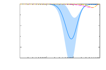
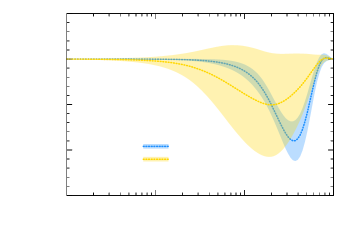
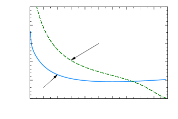
In Fig. 1, we have compared the results obtained from the WACS data Kroll:2017hym (dashed and dashed-dotted curves) for up valence $\widetilde{H}_{v}^{u}$ (up panel) and down valence $\widetilde{H}_{v}^{d}$ (bottom panel) polarized GPDs at $t=-4$ GeV² with our previous work Hashamipour:2019pgy (HGG19) that included only the AFF data (solid curve). As can be seen, there are considerable differences between two approaches. To be more precise, for both valence polarized GPDs, Kroll’s results are more inclined to larger $x$ so that they peaked at $x\sim 0.5$, while HGG19 results peaked at $x\sim 0.1$. This exactly indicates the impact of WACS data on polarized GPDs $\widetilde{H}$, especially at larger values of $-t$. Another point which should be noted is that for the case of $\widetilde{H}_{v}^{d}$, our previous result has a greater magnitude compared to Kroll’s result, while both of them have almost same magnitude for the case of $\widetilde{H}_{v}^{u}$. As we shall explain in details later, we showed in our previous work Hashamipour:2019pgy that the final results are not very sensitive to the choice of PPDFs set used, i.e., DSSV08 deFlorian:2009vb and NNPDFpol1.1 Nocera:2014gqa .Therefore, the different PPDFs used in these two works (Kroll used DSSV08 deFlorian:2009vb , but we used NNPDFpol1.1 Nocera:2014gqa ) cannot lead to such differences, and the resolution must lie elsewhere. As we shall show, performing a simultaneous analysis of AFF and WACS data leads to an improved polarized GPDs $\widetilde{H}$ which differs from the corresponding ones obtained by analyzing AFF and WACS data separately.

Figure 1: A comparison between the Kroll’s results Kroll:2017hym (dashed and dashed-dotted curves) for $\widetilde{H}_{v}^{u}$ (up panel) and $\widetilde{H}_{v}^{d}$ (bottom panel) valence GPDs at $t=-4$ GeV², and corresponding ones from HGG19 analysis Hashamipour:2019pgy (solid curve).

This paper is organized as follows. In Sec. II, we present the theoretical framework we use in this work to analyze the AFF and WACS data and extract GPDs. To this end, following a brief introduction about GPDs, we first review the physics of the theoretical calculation of the nucleon AFF and WACS cross section. Then, we introduce the DFJK model which is used for calculating (polarized) GPDs using predetermined (polarized) PDFs as input. We discuss also the impact parameter dependent PDFs and nucleon helicity flip distribution $E$. In Sec. III, we specify the experimental data included in our analysis and describe our procedure of data selection. Sec. IV is devoted to presenting the results obtained using various scenarios for theoretical calculation of WACS cross section and also changing input PDFs. The extracted GPDs from different analyses are compared to final GPDs corresponding to the analysis with the lowest value of $\chi^{2}$. Some comparisons between the theoretical predictions obtained using the final GPDs and the experimental data included in the analysis are also presented. Finally, by calculating the distribution in the transverse plane of valence quarks, both in an unpolarized and in a transversely polarized proton, we present our results for ‘proton tomography’. We summarize our results and conclusions in Sec. V.

II Theoretical Framework

As pointed out before, GPDs are nonperturbative objects describing soft dynamics inside hadrons. They are in a sense generalization of both FFs and PDFs. Although GPDs cannot be calculated from perturbative QCD, they can be extracted using the standard $\chi^{2}$ analysis of the related experimental data, thanks to the factorization theorem. In this section, we are going to review some of their features together with their relation to the nucleon AFF, WACS cross section, and Impact parameter dependent PDFs. We also we discuss various Ansatzes for GPDs suggested by DFJK Diehl:2004cx ; Diehl:2007uc ; Diehl:2013xca . Here, just like our previous analysis Hashamipour:2019pgy , we use the convention of Ji Ji:1996ek for GPDs, in which $H$, $E$, $\widetilde{H}$ and $\widetilde{E}$ are defined as Belitsky:2005qn ; Diehl:2003ny :

$$\frac{1}{2}\int\frac{dz^{-}}{2\pi}\,e^{ixP^{+}z^{-}}\langle p^{\prime}|\,\bar{q}(-\frac{1}{2}z)\,\gamma^{+}q(\frac{1}{2}z)\,|p\rangle\Big{|}_{\begin{subarray}{c}z^{+}=0,\\ \bm{z_{\perp}=0}\end{subarray}}$$

$$=\frac{1}{2P^{+}}\left[H^{q}(x,\xi,t)\,\bar{u}(p^{\prime})\gamma^{+}u(p)\right.$$

$$\left.+E^{q}(x,\xi,t)\,\bar{u}(p^{\prime})\frac{i\sigma^{+\alpha}\Delta_{\alpha}}{2m}u(p)\,\right],$$

$$\frac{1}{2}\int\frac{dz^{-}}{2\pi}\,e^{ixP^{+}z^{-}}\langle p^{\prime}|\,\bar{q}(-\frac{1}{2}z)\,\gamma^{+}\gamma_{5}\,q(\frac{1}{2}z)\,|p\rangle\Big{|}_{\begin{subarray}{c}z^{+}=0,\\ \bm{z_{\perp}=0}\end{subarray}}$$

$$=\frac{1}{2P^{+}}\left[\widetilde{H}^{q}(x,\xi,t)\,\bar{u}(p^{\prime})\gamma^{+}\gamma_{5}u(p)\right.$$

$$\left.+\widetilde{E}^{q}(x,\xi,t)\,\bar{u}(p^{\prime})\frac{\gamma_{5}\Delta^{+}}{2m}u(p)\,\right],$$ (1)

where $z=\left(z^{+},\bm{z_{\perp}},z^{-}\right)$. As it is evident from Eq. (II), GPDs depend on three kinematical variables, $x$, $\xi$ and $t$. The first one is the well-known Bjorken scaling variable $x=\frac{Q^{2}}{2p\cdot q}$, with photon virtuality $Q^{2}$, which can be interpreted as the average of momentum fractions of active quarks. The other longitudinal variable $\xi=\frac{p^{+}-p^{\prime+}}{p^{+}+p^{\prime+}}$, which is called ‘skewness’, does not appear in PDFs. The last argument is $t=(p^{\prime}-p)^{2}=\Delta^{2}$, i.e. the squared of the momentum transferred to the proton target.

We can express valence GPDs $H_{v}^{q}$ of flavor $q$ in terms of quark GPDs $H^{q}$ as

$$H_{v}^{q}(x,t)=H^{q}(x,\xi=0,t)+H^{q}(-x,\xi=0,t),$$ (2)

with $H^{q}(-x,\xi=0,t)=-H^{\bar{q}}(x,\xi=0,t)$. An analogous relation holds for the valence GPDs $E_{v}^{q}$. The situation is somewhat different for the case of valence polarized GPDs $\widetilde{H}^{q}_{v}$ so that we have

$$\widetilde{H}^{q}_{v}(x,t)=\widetilde{H}^{q}(x,\xi=0,t)-\widetilde{H}^{q}(-x,\xi=0,t),$$ (3)

with $\widetilde{H}^{q}(-x,\xi=0,t)=\widetilde{H}^{\bar{q}}(x,\xi=0,t)$.

Since we are going to analyze the nucleon AFF and WACS data to put constraints on GPDs, it is worthwhile to review the relevant theoretical framework. To this aim, we will first describe the important sum rules which relate GPDs and FFs in Subsection II.1, with more emphasis on the nucleon AFF. The formulas and relations needed for theoretical calculations of the WACS cross section are given in Subsection II.2. In Subsection II.3, we introduce our phenomenological framework for modeling GPDs and performing a global analysis of AFF and WACS data. Finally, we introduce the impact parameter dependent PDFs and nucleon helicity flip distribution $E$ that we use for proton tomography in Subsection II.4.

II.1 Axial Form Factor

There are a certain number of sum rules that relate nucleon FFs to GPDs by exploiting the fact that they are different moments of GPDs Diehl:2013xca . The Dirac and Pauli form factors, $F_{1}$ and $F_{2}$, for example, can be written as follows

$$F_{i}^{p}=e_{u}F_{i}^{u}+e_{d}F_{i}^{d}+e_{s}F_{i}^{s},$$

$$F_{i}^{n}=e_{u}F_{i}^{d}+e_{d}F_{i}^{u}+e_{s}F_{i}^{s},$$ (4)

where $F_{i}^{q}$ for $i=1(2)$ is the contribution of quark flavor $q$ to the Dirac (Pauli) FF of the proton ($F^{p}$) or neutron ($F^{n}$), respectively. Note that $e_{q}$ is the charge of the quark in units of the positron charge. On the other hand, we can write the flavor form factors $F_{i}^{q}$ in terms of the proton valence GPDs $H_{v}$ and $E_{v}$ for unpolarized quarks of flavor $q$ as

$$F_{1}^{q}(t)=\int_{0}^{1}dx~{}H_{v}^{q}(x,t),$$

$$F_{2}^{q}(t)=\int_{0}^{1}dx~{}E_{v}^{q}(x,t).$$ (5)

It is worth noting that the Lorentz invariance makes the result independent of skewness $\xi$, so we choose zero-skewness GPDs and omit this variable from now on.

In analogy with the Dirac and Pauli FFs, the nucleon AFF can be expressed in terms of polarized GPDs as Diehl:2013xca

$$G_{A}(t)= \int_{0}^{1}dx\left[\widetilde{H}^{u}_{v}(x,t)-\widetilde{H}^{d}_{v}(x,t)\right]+$$

$$2 \int_{0}^{1}dx\left[\widetilde{H}^{\bar{u}}(x,t)-\widetilde{H}^{\bar{d}}(x,t)\right].$$ (6)

As it can be readily seen from Eq. (6), contrary to Pauli and Dirac FFs, the AFF involves some contributions from the sea quarks. We examined these contributions in our previous study Hashamipour:2019pgy and found that they are not significant compared to the valence contributions, but not negligible. It is worth mentioning that, from the conceptual point of view, $\int_{0}^{1}dx~{}\widetilde{H}^{q}(x,t)$ is the intrinsic spin contribution of quark $q$ to the spin of proton. Some other moments of GPDs can be related to the matrix elements of energy-momentum tensor.

II.2 Wide-angle Compton scattering

As mentioned in the Introduction, we are going to study the impact of WACS data on the behavior of GPDs, especially at larger values of $-t$, by analyzing them simultaneously with AFF data. To this end, in this subsection we briefly review the relations and formulae needed to calculate the WACS amplitudes and cross section. If one considers a regime in which the Mandelstam variables $s$, $-t$, and $-u$ are large compared to the QCD scale parameter $\Lambda$, the (unpolarized) WACS cross section can be written as Huang:2001ej ,

$${}\frac{d\sigma}{dt}= \frac{1}{32\pi\left(s-m^{2}\right)^{2}}\left\{\left|\Phi_{1}\right|^{2}+\left|\Phi_{2}\right|^{2}+2\left|\Phi_{3}\right|^{2}+2\left|\Phi_{4}\right|^{2}\right.$$

$$\left.+\left|\Phi_{5}\right|^{2}+\left|\Phi_{6}\right|^{2}\right\},$$ (7)

where $\Phi_{1},\dots,\Phi_{6}$ represent the six independent $\Phi_{\mu^{\prime}\nu^{\prime},\mu\nu}$ which denote the center-of-mass-system (c.m.s.) helicity amplitudes. In fact, 16 ($2^{4}$) amplitudes contribute to the Compton scattering theoretically. However, the parity and time-reversal invariance lead to the following relations among them which reduce the number of independent amplitudes to six Kroll:2017hym ,

$${}\Phi_{-\mu^{\prime}-\nu^{\prime},-\mu-\nu}=\Phi_{\mu\nu,\mu^{\prime}\nu^{\prime}}=\left(-1\right)^{\mu-\nu-\mu^{\prime}+\nu}\Phi_{\mu^{\prime}\nu^{\prime},\mu\nu}.$$ (8)

Below, we show the convention that we have used  Huang:2001ej ,

$${}\Phi_{1}= \Phi_{++,++},\quad \Phi_{2}= \Phi_{--,++},\quad \Phi_{3}= \Phi_{-+,++},$$

$$\Phi_{4}= \Phi_{+-,++},\quad \Phi_{5}= \Phi_{-+,-+},\quad \Phi_{6}= \Phi_{-+,+-}.$$ (9)

It can be shown that, in the handbag approach, the derivation of the Compton amplitudes is inherently simpler using the light-cone helicity basis. On the other hand, the ordinary photon-proton c.m.s. helicity basis is more convenient for comparison with experimental and other theoretical results. The relation between the light-cone helicity amplitudes, $\mathcal{M}_{\mu^{\prime}\nu^{\prime},\mu\nu}$, and the c.m.s. helicity amplitudes, $\Phi_{\mu^{\prime}\nu^{\prime},\mu\nu}$, is as follows Huang:2001ej ,

$${}\Phi_{\mu^{\prime}\nu^{\prime},\mu\nu}= \mathcal{M}_{\mu^{\prime}\nu^{\prime},\mu\nu}+\frac{\beta}{2}\left[(-1)^{\frac{1}{2}-\nu^{\prime}}\mathcal{M}_{\mu^{\prime}-\nu^{\prime},\mu\nu}\right.$$

$$\left.+(-1)^{\frac{1}{2}+\nu}\mathcal{M}_{\mu^{\prime}\nu^{\prime},\mu-\nu}\right],$$ (10)

where,

$${}\beta=\frac{2m}{\sqrt{s}}\frac{\sqrt{-t}}{\sqrt{s}+\sqrt{-u}}.$$ (11)

In the handbag approximation, the WACS amplitudes, $\mathcal{M}_{\mu^{\prime}\nu^{\prime},\mu\nu}$, can be factored into two parts: the (hard) parton level subprocess amplitudes, $\mathcal{H}_{\mu^{\prime}\nu^{\prime},\mu\nu}$, and the (soft) form factors of the proton, $R_{i}$, as follows Huang:2001ej ,

$${}\mathcal{M}_{\mu^{\prime}+,\mu+}(s,t)=$$

$$2\pi\alpha_{\mathrm{em}}\left[\mathcal{H}_{\mu^{\prime}+,\mu+}(\hat{s},\hat{t})\left(R_{V}(t)+R_{A}(t)\right)\right.$$

$$\left.+\mathcal{H}_{\mu^{\prime}+,\mu+}(\hat{s},\hat{t})\right(R_{V}(t)-R_{A}(t)\left)\right],$$

$$\mathcal{M}_{\mu^{\prime}-,\mu-}(s,t)=$$

$$\pi\alpha_{\mathrm{em}}\frac{\sqrt{-t}}{m}R_{T}(t)\left[\mathcal{H}_{\mu^{\prime}+,\mu+}(\hat{s},\hat{t})\right.$$

$$\left.+\mathcal{H}_{\mu^{\prime}+,\mu+}(\hat{s},\hat{t})\right].$$ (12)

Note that the $\mathcal{M}$ and $\mathcal{H}$ also satisfy Eq. (8). We have denoted the Mandelstam variables for the photon-parton subprocess by $\hat{s}$, $\hat{t}$, and $\hat{u}$, and for the overall photon-proton reaction by $s$, $t$, $u$. In the above relations, $\mu$ and $\mu^{\prime}$ refer to the polarization of photons before and after interaction. The explicit helicities in the light-cone helicity amplitudes, $\mathcal{M}$, and the subprocess amplitudes, $\mathcal{H}$, represent the polarizations of the proton and active quarks, respectively. The hard scattering amplitudes, $\mathcal{H}_{\mu^{\prime}\nu^{\prime},\mu\nu}$, associated with $\gamma q\rightarrow\gamma q$ subprocess can be calculated in the perturbative QCD. To the leading order (LO) they read Huang:2001ej ,

$${}\mathcal{H}_{++,++}^{\mathrm{LO}}=2\sqrt{\frac{\hat{s}}{-\hat{u}}},\quad\mathcal{H}_{-+,-+}^{\mathrm{LO}}=2\sqrt{\frac{-\hat{u}}{\hat{s}}},\quad\mathcal{H}_{-+,++}^{\mathrm{LO}}=0,$$ (13)

while they have more complicated forms at the next-to-leading order (NLO),

$${}\mathcal{H}_{++,++}^{\mathrm{NLO}} =\frac{\alpha_{\mathrm{s}}}{2\pi}C_{F}\left\{\frac{\pi^{2}}{3}-7+\frac{2\hat{t}-\hat{s}}{\hat{s}}\log\frac{\hat{t}}{\hat{u}}+\log^{2}\frac{-\hat{t}}{\hat{s}}\right.$$

$$\left.+\frac{\hat{t}^{2}}{\hat{s}^{2}}\left(\log^{2}\frac{\hat{t}}{\hat{u}}+\pi^{2}\right)-2i\pi\log\frac{-\hat{t}}{\hat{s}}\right\}\sqrt{\frac{\hat{s}}{-\hat{u}}},$$

$$\mathcal{H}_{-+,-+}^{\mathrm{NLO}} =\frac{\alpha_{\mathrm{s}}}{2\pi}C_{F}\left\{\frac{4}{3}\pi^{2}-7+\frac{2\hat{t}-\hat{u}}{\hat{u}}\log\frac{-\hat{t}}{\hat{s}}+\frac{\hat{t}^{2}}{\hat{u}^{2}}\log^{2}\frac{-\hat{t}}{\hat{s}}\right.$$

$$\left.+\log^{2}\frac{\hat{t}}{\hat{u}}-2i\pi\left(\frac{2\hat{t}-\hat{u}}{2\hat{u}}+\frac{\hat{t}^{2}}{\hat{u}^{2}}\log\frac{-\hat{t}}{\hat{s}}\right)\right\}\sqrt{\frac{-\hat{u}}{\hat{s}}},$$

$$\mathcal{H}_{-+,++}^{\mathrm{NLO}} =-\frac{\alpha_{\mathrm{s}}}{2\pi}C_{F}\left\{\sqrt{\frac{-\hat{u}}{\hat{s}}}+\sqrt{\frac{\hat{s}}{-\hat{u}}}\right\}.$$ (14)

Where $C_{F}=4/3$ is QCD color factor.

The soft form factors of the proton in Eq. (II.2) are denoted by $R_{i}$, where the subscript $i=V,A,T$ stands for vector, axial, and transverse, respectively. They can be expressed as follows,

$${}R_{V}^{q}(t)= \int_{-1}^{1}\frac{dx}{x}H^{q}(x,t),$$

$$R_{A}^{q}(t)= \int_{-1}^{1}\frac{dx}{x}\ \mathrm{sign}(x)\widetilde{H}^{q}(x,t),$$

$$R_{T}^{q}(t)= \int_{-1}^{1}\frac{dx}{x}E^{q}(x,t).$$ (15)

Indeed, as mentioned before, the skewness dependence drops in $x$ integration due to the Lorentz invariance so that one can safely omit this variable and take the GPDs at $\xi=0$. Now, using the above relations, one can obtain the full form factors from the individual quark contributions as follows,

$${}R_{i}(t)=\sum_{q}e^{2}_{q}R_{i}^{q}(t),$$ (16)

where $e_{q}$ is the charge of quark $q$ in units of positron charge. More explicitly, we have

$${}R_{V}(t)= \sum_{q}e^{2}_{q}\int_{0}^{1}\frac{dx}{x}[H_{v}^{q}(x,t)+2H^{\bar{q}}(x,t)],$$

$$R_{A}(t)= \sum_{q}e^{2}_{q}\int_{0}^{1}\frac{dx}{x}[\widetilde{H}_{v}^{q}(x,t)+2\widetilde{H}^{\bar{q}}(x,t)],$$

$$R_{T}(t)= \sum_{q}e^{2}_{q}\int_{0}^{1}\frac{dx}{x}[E_{v}^{q}(x,t)+2E^{\bar{q}}(x,t)].$$ (17)

In general, the Mandelstam variables at the partonic level are different from those of the whole process. Following the work of Diehl et al. Diehl:2002ee , and assuming massless quarks, we introduce three scenarios to relate these two sets of variables. If the mass of the proton can be neglected, the matching of the subprocess and full Mandelstam variables is simplest. In this case we have

$${}\mathrm{scenario\ 1:}\quad\hat{s}=s,\quad\hat{t}=t,\quad\hat{u}=u.$$ (18)

In order to estimate the influence of the proton mass, two more scenarios are also introduced:

$$\mathrm{scenario\ 2:}\quad\hat{s}=s-m^{2},\quad\hat{t}=t,\quad\hat{u}=u-m^{2}.$$

$$\mathrm{scenario\ 3:}\quad\hat{s}=s-m^{2},\quad\hat{t}=-\frac{\hat{s}}{2}\left(1-\cos\theta_{\mathrm{cm}}\right),$$

$$\qquad\qquad\qquad\hat{u}=-\hat{s}-\hat{t}.$$ (19)

It is worth noting that, in contrast to scenario 1, the relation $\hat{s}+\hat{t}+\hat{u}=0$ holds in scenarios 2 and 3 even though we do not ignore the nucleon mass, since $s+t+u=2m_{p}^{2}$. Note also that the aforementioned differences in the Mandelstam variables can be regarded as a source of theoretical uncertainty to the results Diehl:2002ee . We will study in detail the effects of considering these different scenarios for calculating the WACS cross section on the quality of the fit in Sec. IV.2.

II.3 Modeling the GPDs

As a result of many theoretical and phenomenological work, there are numerous models Pasquini:2005dk ; Pasquini:2006dv ; Dahiya:2007mt ; Frederico:2009fk ; Mukherjee:2013yf ; Maji:2015vsa and parameterizations Goldstein:2010gu ; Goldstein:2013gra ; Sharma:2016cnf for GPDs such as Radyushkin’s double distributions Radyushkin:1997ki , light-front constituent quark models Frederico:2009fk , and quark-diquark induced parameterization Goldstein:2010gu . Here, as in our previous work Hashamipour:2019pgy , we consider a simple but advantageous Ansatz suggested by DFJK Diehl:2004cx ; Diehl:2007uc ; Diehl:2013xca . This Ansatz expresses the (polarized) GPDs as a product of ordinary (PPDFs) PDFs and an exponential which contains the $t$ dependence of GPDs, regulated with a specific profile function in $x$. This structure is such that, in the forward limit, (polarized) GPDs will reduce to their ordinary (PPDF) PDF equivalents. For example, for positive $x$, the GPD $H$ changes to the usual quark and antiquark densities as $H^{q}(x,0,0)=q(x)$ and $H^{q}(-x,0,0)=\bar{q}(x)$. According to the DFJK Ansatz which gives $x$ and $t$ dependence of GPDs at zero skewness, the valence GPDs $H_{v}^{q}$ can be related to ordinary valence PDFs as

$$H_{v}^{q}(x,t,\mu^{2})=q_{v}(x,\mu^{2})\exp[tf_{q}(x)],$$ (20)

where $\mu$ is the factorization scale at which the partons are resolved, just like the usual quark densities Diehl:2004cx . It should be noted that in Ansatz (20), which has a motivation from Regge theory, the profile function $f_{q}(x)$ in the exponential is $x$-dependent slope of $\partial\left(\log H_{v}^{q}\right)/{\partial t}$ and can have various functional forms. In the simplest form, which we shall refer to as the simple Ansatz, $f_{q}(x)$ is as follows,

$$f_{q}(x)=\alpha^{\prime}(1-x)\log\frac{1}{x},$$ (21)

where $\alpha^{\prime}$ is an adjustable parameter that should be determined from the analysis of the relevant experimental data. In fact, it has been indicated Diehl:2004cx that the low- and high-$x$ behavior of $f_{q}(x)$, as well as the intermediate-$x$ region, can be well characterized by the following forms

$$f_{q}(x)=\alpha^{\prime}(1-x)^{2}\log\frac{1}{x}+B_{q}(1-x)^{2}+A_{q}x(1-x),$$ (22)

and

$$f_{q}(x)=\alpha^{\prime}(1-x)^{3}\log\frac{1}{x}+B_{q}(1-x)^{3}+A_{q}x(1-x)^{2},$$ (23)

where $A_{q}$ and $B_{q}$ are additional adjustable parameters. For example, the above profile functions were used for a fit to the experimental data of the Dirac and Pauli FFs Diehl:2004cx , and also for a phenomenological study of the strange Dirac form factor $F_{1}^{s}$ Diehl:2007uc . It is worth noting that a profile function of the form $\alpha^{\prime}\log(1/x)+B$ is also used for studying the hard exclusive pion electroproduction, where GPDs play a key role Goloskokov:2011rd . However, in our previous work Hashamipour:2019pgy , we studied the effect of using this profile function for analyzing the nucleon AFF data and observed that it will not lead to an improvement in the quality of the fit. Moreover, we indicated that among the profile functions (21), (22), and (23), the last one can lead to lower values for the $\chi^{2}$ divided by the number of degrees of freedom, $\chi^{2}/\mathrm{d.o.f.}$, by considering the same $A_{v}$ and $B_{v}$ parameters for valence quarks and setting the corresponding sea quark parameters equal to zero.

According to DFJK model, an Ansatz similar to that shown in Eq. (20) can also be considered for the valence polarized GPDs $\widetilde{H}^{q}_{v}$, so that they can be related to valence PPDFs, $\Delta q_{v}(x)\equiv q^{+}(x)-q^{-}(x)$, as following

$$\widetilde{H}^{q}_{v}(x,t,\mu^{2})=\Delta q_{v}(x,\mu^{2})\exp[t\widetilde{f}_{q}(x)],$$ (24)

where $\widetilde{f}_{q}(x)$ is the corresponding profile function which again can have a simple form like Eq. (21), or a complex form with more adjustable parameters like Eq. (22) or (23).

In the present work, we are going to analyze both the AFF and WACS data simultaneously to determine GPDs and also compare the results with the previous ones obtained by analyzing the AFF data solely Hashamipour:2019pgy , in order to investigate the impact of WACS data on the extracted densities, especially at larger values of $-t$. To this end, we use the DFJK Ansatzes of Eqs. (20) and (24) for the unpolarized and polarized GPDs $H$ and $\widetilde{H}$, respectively. Moreover, for simplicity, we use these Ansatzes both for the valence and sea quark contributions as before Hashamipour:2019pgy , though the physical motivation to use them for the sea contributions is not as strong as that of the valence ones Diehl:2013xca . As is expected and we shall show, the contributions of the sea are not significant compared to those that come from the valence sector. Another point which should be mentioned is that, according to Eq. (6), only the polarized GPDs $\widetilde{H}$ contribute to the AFF, while for the case of WACS cross section three kinds of GPDs, namely $H$, $\widetilde{H}$, and $E$, are involved through the soft FFs of the proton $R_{V}$, $R_{A}$, and $R_{T}$, respectively (see Eq. (II.2)). Since the contribution of the $R_{T}$ in WACS cross section is considerably smaller than $R_{V}$ and $R_{A}$ (see Fig. 24 of Ref. Diehl:2013xca ), we fix the GPDs $E_{v}^{q}(x,t)$ and $E^{\bar{q}}(x,t)$ from the analysis of Ref. Diehl:2004cx , and just parameterize the $H$ and $\widetilde{H}$ GPDs. Consequently, the constraints on $H$ come just from the WACS data, while $\widetilde{H}$ can be constrained by both the AFF and WACS data.

II.4 Impact parameter dependent PDFs and nucleon helicity flip distribution $E$

As is well known, the Fourier transform of GPDs at zero skewness, $\xi=0$, which are called impact parameter dependent PDFs, satisfy positivity constraints so that one can associate the physical interpretation of a probability density with them. Indeed, they describe the distribution of partons in the transverse plane Diehl:2004cx ; Burkardt:2000za ; Burkardt:2002hr . Therefore, one can relate GPDs $H$ and $\widetilde{H}$ to the impact parameter distribution of unpolarized quarks in an unpolarized nucleon and the distribution of longitudinally polarized quarks in a longitudinally polarized nucleon, respectively. Moreover, $E$ is related to the distortion of the unpolarized quark distribution in the transverse plane when the nucleon has transverse polarization. In fact, the distribution $E_{v}^{q}(x,\xi,t)$ at zero skewness describes proton-helicity flip in a frame where the proton moves fast Burkardt:2002hr , i.e., in the infinite momentum frame.

As mentioned, one can achieve a density interpretation of GPDs at $\xi=0$ in the mixed representation of longitudinal momentum and transverse position in the infinite-momentum frame Burkardt:2000za ; Burkardt:2002hr . For instance, the impact parameter dependent parton distribution related to $H$ can be defined as follows Diehl:2004cx

$$q_{v}(x,\bm{b})=\int\frac{\mathrm{d}^{2}\bm{\mathbold{\Delta}}}{(2\pi)^{2}}\,\mathrm{e}^{-\mathrm{i}\bm{b}.\mathbold{\Delta}}\,H_{v}^{q}(x,t=-\mathbold{\Delta}^{2}).$$ (25)

From the physical point of view, $q_{v}(x,\bm{b})$ gives the probability of finding a quark with longitudinal momentum fraction $x$ and impact parameter $\bm{b}=(b^{x},b^{y})$ minus the probability of finding an antiquark with the same $x$ and $\bm{b}$. Here we have adhered to the usual convention of using the $x$ and $y$ superscripts to denote the $x$ and $y$ axes in the transverse plane, where the distinction between the former and the Bjorken $x$ is implicit. Actually, the impact parameter $\bm{b}$ in $q_{v}(x,\bm{b})$ is the transverse distance between the struck parton and the center of momentum of the hadron Burkardt:2002hr . We use the boldface notation for the two-dimensional vectors in the transverse plane. We can obtain the average of impact parameter squared from $q_{v}(x,\bm{b})$ as follows Diehl:2004cx

$$\langle\bm{b}^{2}\rangle^{q}_{x}=\frac{\int\mathrm{d}^{2}\bm{b}\,\bm{b}^{2}\,q_{v}(x,\bm{b})}{\int\mathrm{d}^{2}\bm{b}\,q_{v}(x,\bm{b})}=4\frac{\partial}{\partial t}\log H_{v}^{q}(x,t)\Bigg{|}_{t=0},$$ (26)

which is to be calculated at fixed $x$. It is worth noting that the use of an exponential Ansatz for the $t$-dependence of unpolarized GPDs, given in Eq. (20), guarantees that $q_{v}(x,\bm{b})$ is positive. An estimate of the size of the hadron can be provided using the relative distance between the struck parton and the spectator system, $\bm{b}/(1-x)$. As explained in Ref. Diehl:2004cx , the average square of this distance is calculated from

$$d_{q}^{2}(x)=\frac{\langle\bm{b}^{2}\rangle^{q}_{x}}{(1-x)^{2}},$$ (27)

so that $d_{q}$ provides a lower limit for the transverse size of the hadron.

It can be shown that Burkardt:2002hr if one changes basis from longitudinal to transverse polarization states of the proton, $E^{q}_{v}$ has also a probability interpretation in impact parameter space. In analogy to Eq. (25), the probability to find an unpolarized quark with momentum fraction $x$ and impact parameter $\bm{b}$ in a transversly polarized proton, minus the probability to find an antiquark with the same $x$ and $\bm{b}$ is given by the distribution Burkardt:2002hr ,

$$q_{v}^{X}(x,\bm{b})=q_{v}(x,\bm{b})-\frac{b^{y}}{m}\,\frac{\partial}{\partial\bm{b}^{2}}\,e_{v}^{q}(x,\bm{b}),$$ (28)

where the Fourier transform $e_{v}^{q}(x,\bm{b})$ is given by,

$$e_{v}^{q}(x,\bm{b})=\int\frac{\mathrm{d}^{2}\bm{\mathbold{\Delta}}}{(2\pi)^{2}}\,\mathrm{e}^{-\mathrm{i}\bm{b}.\mathbold{\Delta}}\,E_{v}^{q}(x,t=-\mathbold{\Delta}^{2}).$$ (29)

Eq. (28) clearly indicates that transverse target polarization induces a shift in the quark distribution along the $y$-axis. One can consider the classical picture of the polarized proton as a sphere that rotates about the $x$-axis and moves in the $z$-direction to better understand such effect Burkardt:2002hr ; Belitsky:2003nz . The average of this shift is given by

$$\langle b^{y}\rangle^{q}_{x}=\frac{\int\mathrm{d}^{2}\mathbold{b}\;b^{y}\,q_{v}^{X}(x,\mathbold{b})}{\int\mathrm{d}^{2}\mathbold{b}\,q_{v}^{X}(x,\mathbold{b})}=\frac{1}{2m}\,\frac{E_{v}^{q}(x,0)}{H_{v}^{q}(x,0)}\,.$$ (30)

Note that, in this case, the corresponding shift for the distance between the struck quark and the spectator system is as follows

$$s_{q}(x)=\frac{\langle b^{y}\rangle^{q}_{x}}{1-x},$$ (31)

which is comparable to the distance function $d_{q}(x)$ in Eq. (27). An important property of the impact parameter space distributions is that they satisfy certain inequalities Burkardt:2003ck , ensuring that the quark densities for various combinations of proton and quark spins are positive. By calculating the impact parameter dependent PDFs according to the above formulations, we can present the proton tomography that illustrates the interplay between longitudinal and transverse partonic degrees of freedom in the proton.

In the following, by performing various $\chi^{2}$ analyses of the AFF and WACS data at NLO, we determine the optimum values of not only the free parameters of the profile function (23), in particular $\alpha^{\prime}$, but also the scale $\mu$ at which the PDFs and PPDFs are chosen in Ansatzes (20) and (24), respectively.

It should be noted that the Regge phenomenology and various studies have indicated that the value of $\alpha^{\prime}$ should be close to 1 Diehl:2004cx ; Diehl:2007uc ; Diehl:2013xca . Although our final analysis of the AFF data Hashamipour:2019pgy also confirmed this value, it led to a smaller value for $\mu$ (1 GeV) than that which has been considered in Refs. Diehl:2004cx ; Diehl:2007uc ; Diehl:2013xca (2 GeV). So, it is of interest to investigate to what extent the inclusion of WACS data in the analysis affects the values of $\alpha^{\prime}$ and $\mu$, along with the shape of extracted GPDs.

III Data selection

As mentioned before, our goal is analyzing the AFF and WACS experimental data simultaneously, in order to determine quark GPDs $H$ and $\widetilde{H}$ within the theoretical framework described in Sec. II. To this aim, an important step is gathering the available experimental data for both processes. Contrary to the electromagnetic nucleon FFs which their extraction has a long history and remains a popular field of experimental research (see Ref. Diehl:2013xca for an overview), there are fewer measurements of the nucleon AFF. In fact, at the present, one can only use the (anti)neutrino scattering off nucleons and charged pion electroproduction to determine nucleon AFF. Most of the available measurements for the nucleon AFF obtained from charged pion electroproduction have been reviewed and discussed in Refs. Bernard:2001rs ; Schindler:2006jq , and for the case of (anti)neutrino scattering experiments, one can refer to the data obtained from MiniBooNE experiments Butkevich:2013vva . Similarly, there are not many measurements of WACS cross section. As a comprehensive effort, one can refer to the measurements by the Jefferson Lab Hall A Collaboration Danagoulian:2007gs which include 25 kinematic settings over the range $s=5-11$ GeV² and $-t=2-7$ GeV².

In our previous work Hashamipour:2019pgy , we used the available data of nucleon AFF to determine polarized GPDs $\widetilde{H}$ using the DFJK Ansatz of Eq. (24) and considering various profile functions. Although there were 84 data points from Refs. Butkevich:2013vva ; Amaldi:1970tg ; Amaldi:1972vf ; Bloom:1973fn ; Brauel:1973cw ; DelGuerra:1975uiy ; DelGuerra:1976uj ; Joos:1976ng ; Esaulov:1978ed ; Choi:1993vt ; Choi:1993 , we formed a “reduced” data set by removing data points with the same value of $-t$ and retaining the most accurate ones which reduced the number of data to 40 (see Fig. 1 of Ref. Hashamipour:2019pgy ). However, because of the inconsistencies in data sets (our investigations indicated that these inconsistencies are not due to the normalization), analyzing the reduced set led to a large value for the $\chi^{2}$ divided by the number of degrees of freedom, $\chi^{2}/\mathrm{d.o.f.}$, of the order of 4.5. In this work, we further reduce our AFF data by removing the older data sets and only use data from Refs. Butkevich:2013vva ; Esaulov:1978ed ; DelGuerra:1975uiy ; Bloom:1973fn ; Joos:1976ng ; Choi:1993vt . Consequently, the number of data points of the nucleon AFF included in our new reduced set is 34 which cover the range $0.025<-t<1.84$ GeV². Another important point which should be mentioned is that we use data as $G_{A}(-t)$, just like before, while the original data are given as $G_{A}(-t)/G_{A}(0)$. In fact, as we have indicated, the quantity $G_{A}(-t)/G_{A}(0)$ cannot put any constraint on the value of scale $\mu$ at which PPDFs are chosen, and hence the resulting value for $\alpha^{\prime}$ is not very reliable in such cases. For extracting $G_{A}(-t)$ from original $G_{A}(-t)/G_{A}(0)$ data, we use the latest value of $G_{A}(0)$ (axial charge $g_{A}$) from PDG Tanabashi:2018oca , i.e. $g_{A}=1.2723\pm 0.0023$.

For the case of WACS data, we use the measurements by the Jefferson Lab Hall A Collaboration Danagoulian:2007gs with four values of $s$, namely $s=4.82,6.79,8.90,$ and 10.92 GeV². Their measurements contain 25 data points which cover a wide range of $-t$, i.e. $1.65<-t<6.46$ GeV². As can be seen, although the AFF data can be used to constrain polarized GPDs mainly at smaller values of $-t$, some important information can also be obtained from WACS data, which mainly constrain the large $-t$ behavior of $\widetilde{H}$. In the next section, we perform various analyses on the aforementioned AFF and WACS data simultaneously to study in detail the possible changes in the extracted GPDs, and also the values of $\alpha^{\prime}$ and $\mu$.

IV Results and Discussions

In the previous sections, we have introduced the theoretical framework and experimental data which we use in the present study to determine GPDs $H$ and $\widetilde{H}$. In this section, we perform various analyses of the AFF and WACS data at NLO using different approaches to find the best one which leads to lowest $\chi^{2}$ with minimum number of parameters. In this regard, we first do a parameterization scan (similar to what was done in Ref. Aaron:2009aa ) to find the optimum form of profile function (23) for each flavor of $H$ and $\widetilde{H}$ GPDs, and reduce the number of free parameters as far as possible. Then, since the theoretical calculation of WACS cross section can be done within the various scenarios (see Sec. II.2), we perform three separate analyses in order to find the best scenario which leads to lowest $\chi^{2}$ for AFF and WACS data simultaneously, and thus the best agreement between the theoretical predictions and experimental data. As mentioned before, in our previous work Hashamipour:2019pgy we showed that if $\widetilde{H}$ is represented by the Ansatz of Eq. (24) for calculating $G_{A}$, the final results will not be very sensitive to the choice of PPDFs set. In this work, since the theoretical calculation of WACS cross section needs $H$ and hence the unpolarized PDFs according to Ansatz (20), we perform various analyses using different sets of PDFs to study the sensitivity of the results to changes of PDFs. After finding the optimum form of profile function (23) for each flavor, the best scenario for calculating WACS cross section, and the most compatible PDFs set, we present the final results of the extracted GPDs $H$ and $\widetilde{H}$ along with their uncertainties. Some comparisons between the theoretical calculations obtained using the final GPDs and the experimental data included in the analysis are also presented. Finally, we present some tomography plots by calculating the impact parameter dependent PDFs introduced in Sec. II.4. It should be noted that we use the CERN program MINUIT James:1975dr for doing the optimization and finding the best values of the fit parameters. Wherever needed, we use the LHAPDF package Buckley:2014ana to access a specific PDFs or PPDFs set and also the value of the strong coupling constant $\alpha_{s}(\mu)$.

IV.1 Parameterization scan

As mentioned before, in our previous study Hashamipour:2019pgy , we used Ansatz (24) to analyze AFF data and determine polarized GPDs $\widetilde{H}$. We indicated that considering a more flexible profile function like Eq. (23) with the same $A_{v}$ and $B_{v}$ parameters for valence quarks and setting the corresponding sea quark parameters equal to zero can lead to a lower value of $\chi^{2}$, as compared to the simple profile function (21). In this work, we are also going to include the WACS data in the analysis and determine simultaneously the unpolarized GPDs $H$ and polarized GPDs $\widetilde{H}$. So, it is necessary to examine the possibility of constraining a more flexible profile function using the available data and reducing the number of free parameters as far as possible. Such a parameterization scan can be done, for example, by following the procedure described in Ref. Aaron:2009aa which was used to find the optimum functional forms of PDFs.

To find the optimum forms of profile function (23) for GPDs $H$ and $\widetilde{H}$, at this stage we analyze the AFF and WACS data described in Sec. III at NLO, using scenario 1 for theoretical calculation of WACS cross section (Eq. (18)), and also taking the cteq6 PDFs Pumplin:2002vw and NNPDFpol1.1 PPDFs Nocera:2014gqa in Ansatzes (20) and (24), respectively. By doing an exhaustive analytical search, we have found that the lowest $\chi^{2}/\mathrm{d.o.f.}$ occurs when one takes the following profile functions for the polarized GPDs $\widetilde{H}_{v}^{u}$, $\widetilde{H}_{v}^{d}$, and $\widetilde{H}^{\bar{q}}$ ($\bar{q}=\bar{u},\bar{d}$),

$$\widetilde{f}_{u_{v}}(x)= \widetilde{\alpha^{\prime}}_{v}(1-x)^{3}\log\frac{1}{x}+\widetilde{B}_{u_{v}}(1-x)^{3}+\widetilde{A}_{u_{v}}x(1-x)^{2},$$

$$\widetilde{f}_{d_{v}}(x)= \widetilde{\alpha^{\prime}}_{v}(1-x)^{3}\log\frac{1}{x},$$

$$\widetilde{f}_{\bar{q}}(x)= \widetilde{\alpha^{\prime}}_{v}(1-x)^{3}\log\frac{1}{x},$$ (32)

which are obtained by considering $\widetilde{\alpha^{\prime}}_{u_{v}}=\widetilde{\alpha^{\prime}}_{d_{v}}=\widetilde{\alpha^{\prime}}_{\bar{q}}=:\widetilde{\alpha^{\prime}}_{v}$, $\widetilde{A}_{d_{v}}=\widetilde{B}_{d_{v}}=0$, and $\widetilde{A}_{\bar{q}}=\widetilde{B}_{\bar{q}}=0$, and the following profile functions for the unpolarized GPDs $H_{v}^{u}$, $H_{v}^{d}$, and $H^{\bar{q}}$

$$f_{u_{v}}(x) = \widetilde{\alpha^{\prime}}_{v}(1-x)^{3}\log\frac{1}{x}+\widetilde{A}_{u_{v}}x(1-x)^{2},$$

$$f_{d_{v}}(x) = \widetilde{\alpha^{\prime}}_{v}(1-x)^{3}\log\frac{1}{x}+\widetilde{A}_{u_{v}}x(1-x)^{2},$$

$$f_{\bar{q}}(x) = \widetilde{\alpha^{\prime}}_{v}(1-x)^{3}\log\frac{1}{x},$$ (33)

which are obtained by considering $\alpha^{\prime}_{u_{v}}=\alpha^{\prime}_{d_{v}}=\alpha^{\prime}_{\bar{q}}=\widetilde{\alpha^{\prime}}_{v}$, $B_{u_{v}}=B_{d_{v}}=0$, $A_{u_{v}}=A_{d_{v}}=\widetilde{A}_{u_{v}}$, and $A_{\bar{q}}=B_{\bar{q}}=0$. With these choices, only three parameters $\widetilde{\alpha^{\prime}}_{v}$, $\widetilde{A}_{u_{v}}$, and $\widetilde{B}_{u_{v}}$ are free and should be determined from the fit. Finally, by also considering the scale $\mu$ as a free parameter, we have four free parameters. Note that, although increasing the number of free parameters can somewhat reduce the value of total $\chi^{2}$, it generically leads to a larger value for $\chi^{2}/\mathrm{d.o.f.}$. Hence, a major limitation at this point in time is the number of experimental data. Nevertheless, the results of the parameterization scan shown in Eq. (IV.1) seem unsatisfactory in the sense that the symmetry between $\widetilde{f}_{u_{v}}(x)$ and $\widetilde{f}_{d_{v}}(x)$ is lost once the parameters $\widetilde{A}_{d_{v}}$ and $\widetilde{B}_{d_{v}}$ are set to zero. Here we adhere to the usual practice of using the results of the parameterization scan as it stands. However, at the end of Sec. IV.4 we perform a new analysis by letting $\widetilde{A}_{d_{v}}$ and $\widetilde{B}_{d_{v}}$ be free parameters in Eq. (IV.1). Upon comparing the results, we show that this has a drastic effect on $\widetilde{H}_{v}^{d}$, which we shall argue to be an improvement, with a decrease of $3\%$ in $\chi^{2}$ and at a cost of only $0.7\%$ increase in $\chi^{2}/\mathrm{d.o.f.}$ We shall compare the results in detail in Sec. IV.4.

IV.2 Study of different scenarios for calculating WACS

As we explained in Sec. II.2, there are three scenarios to relate the Mandelstam variables at partonic level to those of the whole process for calculating the WACS cross section. Using different scenarios may lead to different theoretical predictions for WACS and thus different fit results. In this section, we are going to study this issue to find the best scenario which leads to the lowest value of $\chi^{2}/\mathrm{d.o.f.}$ in analyzing the AFF and WACS data. Note that, like before, we take the cteq6 PDFs Pumplin:2002vw and NNPDFpol1.1 PPDFs Nocera:2014gqa in Ansatzes (20) and (24), respectively to calculate the unpolarized and polarized GPDs $H$ and $\widetilde{H}$.

Table 1 shows the results of three analyses of the experimental data introduced in Sec. III that have been performed using scenarios 1, 2, and 3 described in Sec. II.2. This table contains the list of data sets included in the analysis, along with their related observables and references. For each data set, we have presented the value of $\chi^{2}$ divided by the number of data points, $\chi^{2}$/$N_{\textrm{pts.}}$. The value of $\chi^{2}$/d.o.f. has also been presented for each analysis in the last row of the table. As can be seen, the least $\chi^{2}$/d.o.f. belongs to scenario 3 which is in good agreement with scenario 2. However, scenario 1 leads to the largest $\chi^{2}$/d.o.f., such that its difference with the other scenarios in total $\chi^{2}$ is about 82. Another point should be noted is that the scenarios 1 and 2 lead to significantly different results for AFF data from Refs. Butkevich:2013vva and Esaulov:1978ed , even though they lead to approximately the same $\chi^{2}$/d.o.f..

Table 2 makes a comparison between the optimum parameters of the profile functions (IV.1) and (IV.1), in addition to the scale $\mu^{2}$ at which the PDFs and PPDFs are chosen in Ansatzes (20) and (24), respectively, obtained from three aforementioned analyses. As can be seen, there are considerable differences between the scenarios 1, 2, and 3 so that they lead to considerably different values for parameters $\mu$ and $\alpha^{\prime}$. Note that among these scenarios, only scenario 3 leads to a value for $\alpha^{\prime}$ close to 1 as expected from the previous studies Hashamipour:2019pgy ; Diehl:2004cx ; Diehl:2007uc ; Diehl:2013xca . However, the value of $\mu^{2}$ obtained from scenario 3 (1.5 GeV²) is larger than the corresponding one obtained in our previous work Hashamipour:2019pgy (1 GeV²), where we analyzed the AFF data solely to determined the polarized GPDs $\widetilde{H}$. From now on we consider scenario 3 as the best scenario since it has led to the lowest $\chi^{2}$/d.o.f. (especially for the WACS data) and a more reasonable value for $\alpha^{\prime}$ as compared to scenario 2. In the next subsection, we continue our study by investigating the sensitivity of the results to the PDFs set we choose for calculating the unpolarized GPDs using the Ansatz Eq. (20).

Table 1: The results of three analyses of the experimental data introduced in Sec. III that have been performed using scenarios 1, 2, and 3 described in Sec. II.2.

Observable	Reference	$\chi^{2}$/$N_{\textrm{pts.}}$
		Scenario 1	Scenario 2	Scenario 3
$G_{A}$	Butkevich and Perevalov Butkevich:2013vva	74.78 / 14	54.81 / 14	69.04 / 14
	Del Guerra et al. DelGuerra:1975uiy	2.99 / 4	5.09 / 4	3.36 / 4
	Esaulov et al. Esaulov:1978ed	31.14 / 4	40.75 / 4	33.22 / 4
	Bloom et al. Bloom:1973fn	6.84 / 6	6.09 / 6	6.23 / 6
	Joos et al. Joos:1976ng	16.42 / 5	21.49 / 5	18.90 / 5
	Choi et al. Choi:1993vt	$0.02$ / 1	$0.01$ / 1	$0.01$ / 1
$\frac{d\sigma}{dt}(\mathrm{WACS})$	Danagoulian et al. Danagoulian:2007gs	193.69 / 25	116.13 / 25	113.00 / 25
Total $\chi^{2}/\mathrm{d.o.f.}$		325.88 / 55	244.37 / 55	243.76 / 55

Table 2: The optimum parameters of the profile functions (IV.1) and (IV.1), in addition to the scale $\mu^{2}$ at which the PDFs and PPDFs are chosen, in Ansatzes (20) and (24), respectively, obtained from three analyses of the experimental data of Table 1 that have been performed using scenarios 1, 2, and 3 described in Sec. II.2.

Parameter	Scenario 1	Scenario 2	Scenario 3
$\mu^{2}$	$0.97\pm 0.05$	$1.91\pm 0.32$	$1.50\pm 0.22$
$\widetilde{\alpha^{\prime}}_{v}$	$1.08\pm 0.03$	$0.73\pm 0.02$	$0.99\pm 0.02$
$\widetilde{A}_{u_{v}}$	$3.59\pm 0.17$	$8.30\pm 0.48$	$3.94\pm 0.16$
$\widetilde{B}_{u_{v}}$	$-1.83\pm 0.06$	$-2.12\pm 0.03$	$-1.89\pm 0.03$

IV.3 Dependence on the PDFs

In our previous work Hashamipour:2019pgy , we studied the impact of choosing different sets of PPDFs on the theoretical calculations of the nucleon AFF of Eq. (6), using the Ansatz (24), and showed that the final results were not very sensitive to the choice of PPDFs set. To be more precise, we concluded that the difference between the results obtained for $G_{A}$ using the DSSV08 deFlorian:2009vb and NNPDFpol1.1 Nocera:2014gqa PPDFs was approximately 2% in full range of $-t$ under consideration. In this work, we have also included some new data from the WACS cross section which their theoretical calculations require PDFs according to Eq. (II.2) (through $H$ in $R_{V}$). Therefore, it is also of interest to study the sensitivity of the results to the PDFs set that we choose for calculating the GPDs $H$, and subsequently the WACS cross section.

In the previous subsections, we used the cteq6 PDFs Pumplin:2002vw for doing the parameterization scan and finding the best scenario for calculating the WACS cross section. Now, in order to investigate the effect of PDFs on the fit results, in particular the value of the $\chi^{2}$, the shape of GPDs, and the optimum values of the free parameters, we repeat the analysis of Sec. IV.2 using scenario 3, but this time considering more recent sets of PDFs. To this aim, we use the NLO PDFs from the CT14 Dulat:2015mca , MMHT14 Harland-Lang:2014zoa and NNPDF3.0 Ball:2014uwa and compare their results with each other. The results of these three analyses have been presented in the third, fourth and fifth columns of Table 3, respectively. Overall, we conclude that there are no significant differences between the analyses performed using different PDFs, i.e., the value of total $\chi^{2}$ does not change by more than 1 unit. Table 4 makes a comparison between the optimum parameters obtained from the three aforementioned analyses. As can be seen, the values of the parameters also do not change significantly by choosing different sets of PDFs. However, since the analysis performed using the CT14 PDFs has led to the lowest $\chi^{2}$/d.o.f. according to Table 3, we consider it to be the most suitable. Therefore, our final GPDs are those that have been obtained using scenario 3 for calculating the WACS cross section, and the CT14 PDFs and NNPDFpol1.1 PPDFs Nocera:2014gqa in Ansatzes (20) and (24), respectively. Note that, according to Table 4, our new analysis, which includes the WACS data, confirms the result obtained in our previous work Hashamipour:2019pgy (where we analyzed the AFF data solely) and also other studies Diehl:2004cx ; Diehl:2007uc ; Diehl:2013xca for $\alpha^{\prime}$ ($\alpha^{\prime}\sim 1$). However, the final value of $\mu^{2}$, $\mu^{2}=1.48$ GeV² is larger than our previous work (1 GeV²) and smaller than other studies (4 GeV²) Diehl:2004cx ; Diehl:2007uc ; Diehl:2013xca .

Table 3: The results of three analyses of the experimental data introduced in Sec. III that have been performed using scenario 3 described in Sec. II.2 and the CT14 Dulat:2015mca , MMHT14 Harland-Lang:2014zoa , and NNPDF3.0 Ball:2014uwa PDFs.

Observable	Reference	$\chi^{2}$/$N_{\textrm{pts.}}$
		CT14	MMHT14	NNPDF3.0
$G_{A}$	Butkevich and Perevalov Butkevich:2013vva	68.83 / 14	69.98 / 14	69.86 / 14
	Del Guerra et al. DelGuerra:1975uiy	3.37 / 4	3.31 / 4	3.33 / 4
	Esaulov et al. Esaulov:1978ed	33.32 / 4	32.81 / 4	32.86 / 4
	Bloom et al. Bloom:1973fn	6.21 / 6	6.31 / 6	6.29 / 6
	Joos et alJoos:1976ng	19.01 / 5	18.52 / 5	18.57 / 5
	Choi et al.Choi:1993vt	$0.01$ / 1	$0.01$ / 1	$0.01$ / 1
$\frac{d\sigma}{dt}(\mathrm{WACS})$	Danagoulian et al. Danagoulian:2007gs	111.77 / 25	112.29 / 25	112.48 / 25
Total $\chi^{2}/\mathrm{d.o.f.}$		242.52 / 55	243.23 / 55	243.40 / 55

Table 4: The optimum parameters of the profile functions (IV.1) and (IV.1), in addition to the scale $\mu^{2}$ at which the PDFs and PPDFs are chosen in Ansatzes (20) and (24), respectively, obtained from three analyses of the experimental data of Table 3 that have been performed using scenario 3 described in Sec. II.2 and the CT14 Dulat:2015mca , MMHT14 Harland-Lang:2014zoa and NNPDF3.0 Ball:2014uwa PDFs.

Parameter	CT14	MMHT14	NNPDF3.0
$\mu^{2}$	$1.48\pm 0.21$	$1.52\pm 0.24$	$1.55\pm 0.24$
$\widetilde{\alpha^{\prime}}_{v}$	$0.99\pm 0.02$	$0.99\pm 0.02$	$0.99\pm 0.02$
$\widetilde{A}_{u_{v}}$	$3.90\pm 0.16$	$3.96\pm 0.15$	$3.89\pm 0.15$
$\widetilde{B}_{u_{v}}$	$-1.88\pm 0.03$	$-1.90\pm 0.04$	$-1.87\pm 0.04$

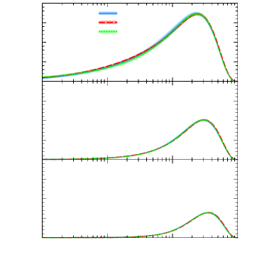
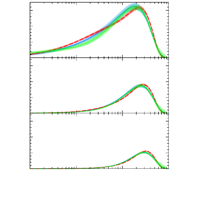
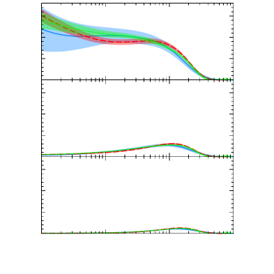
Although there are no significant differences between the results of analyses performed using different sets of PDFs in view of $\chi^{2}$ (Table 3) and parameter (Table 4) values, it is also of interest to compare different GPDs of various flavors obtained from three aforementioned analyses. Top panel of Fig. 2 shows a comparison between the $H_{v}^{u}$ GPDs with their uncertainties obtained using three different sets of NLO PDFs, namely CT14 (blue solid curve), MMHT14 (red dashed curve) and NNPDF3.0 (green dotted curve), and profile function $f_{u_{v}}$ of Eq. (IV.1) with parameters listed in Table 4 at three different values of $t$, $t=0,-0.5$ and $-1$ GeV². As can be seen, the differences between these three sets of GPDs are not very significant. Indeed, we have evaluated them and found that, excluding the regions close to the end points, the differences are less than 5%. However, the results differ more for $H_{v}^{d}$ GPDs which have been compared in the bottom panel of Fig. 2. In fact, in this case, the differences can reach 20% in the same domain as above. An important point which should be mentioned is that, according to Eq. (IV.1), the profile functions $f_{u_{v}}$ and $f_{d_{v}}$ are equal. Therefore, the larger differences observed in the bottom panel of Fig. 2 between the $H_{v}^{d}$ GPDs compared to the $H_{v}^{u}$ GPDs in the top panel come directly from the larger differences in $d_{v}$ PDFs compared to $u_{v}$ PDFs of the CT14, MMHT14 and NNPDF3.0 sets. Figure 3 shows the same comparison of Fig. 2 but for up and down sea quark GPDs $H^{\bar{u}}$ (top panel) and $H^{\bar{d}}$ (bottom panel). As can be seen, the three sets of PDFs produce larger differences for the $H^{\bar{u}}$ and $H^{\bar{d}}$, as compared to their valance counterparts.

Figure 2: A comparison between the up $H_{v}^{u}$ (top panel) and down $H_{v}^{d}$ (bottom panel) unpolarized GPDs with their uncertainties obtained using three different sets of NLO PDFs, namely CT14 (blue solid curve), MMHT14 (red dashed curve) and NNPDF3.0 (green dotted curve), and profile function $f_{u_{v}}$ of Eq. (IV.1) with parameters listed in Table 4 at three different values of $t$, $t=0,-0.5$ and $-1$ GeV².

Figure 3: Same as Fig. 2 but for the up and down sea quark GPDs $H^{\bar{u}}$ (top panel) and $H^{\bar{d}}$ (bottom panel).

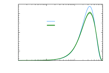
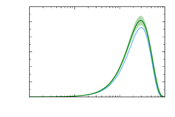
As mentioned before, we consider the GPDs obtained using scenario 3 for calculating the WACS cross section, and the CT14 PDFs and NNPDFpol1.1 PPDFs Nocera:2014gqa in Ansatzes (20) and (24), respectively, as our final GPDs. To check the validity of the results obtained, in Fig. 4 we have compared our GPDs (green solid curve labeled as HGG20) for the up (top panel) and down (bottom panel) valence quarks with the results obtained by Diehl, Feldmann, Jakob, and Kroll (blue dotted curve labeled as DFJK05) Diehl:2004cx . This figure clearly shows a good agreement between the results of these two analyses. Note that in the DFJK05 analysis, the main body of the experimental data was composed of the Dirac and Pauli form factors of the nucleon, while our analysis contains data from the AFF and WACS.

Figure 4: A comparison between our final unpolarized GPDs (green solid curve labeled as HGG20) for the up (top panel) and down (bottom panel) valence quarks with the results obtained by Diehl, Feldmann, Jakob, and Kroll (blue dotted curve labeled as DFJK05) Diehl:2004cx . See Sec. IV.3 for more information.

IV.4 Final polarized GPDs

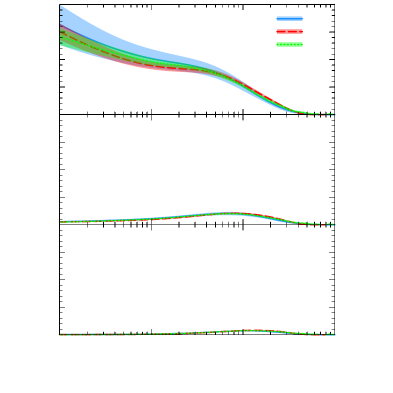
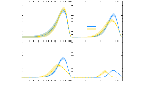
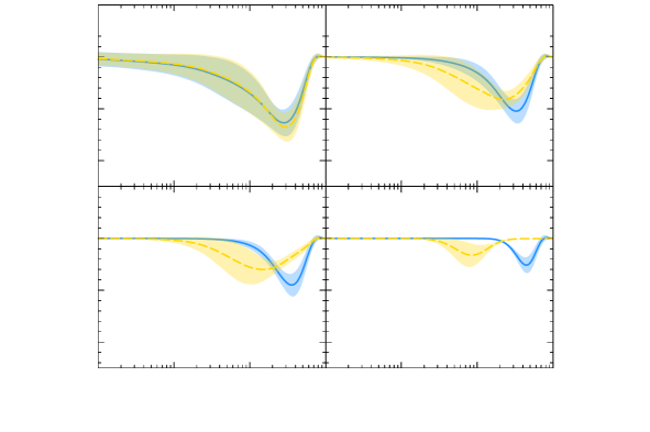
In the previous subsection, we studied in detail the sensitivity of the fit results to the PDFs set that we choose for calculating the GPDs $H$ and WACS cross section. We showed that although there are no significant differences between the analyses performed using different sets of PDFs in view of $\chi^{2}$ and parameter values, the extracted GPDs, especially for the case of down valence and sea quark distributions, differ as functions of $x$. In this subsection, we present our final results for the polarized GPDs $\widetilde{H}_{v}^{u}$, $\widetilde{H}_{v}^{d}$, and $\widetilde{H}^{\bar{q}}$ which can be calculated using the Ansatz (24) and profile functions (IV.1) with parameter values listed in Table 4 for the CT14 analysis and NNPDFpol1.1 as the PPDFs set. Figure 5 shows a comparison between the $\widetilde{H}_{v}^{u}$ (top panel) and $\widetilde{H}_{v}^{d}$ (bottom panel) GPDs with their uncertainties obtained from this work (blue solid curve labeled as HGG20) and our previous work (orange dashed curve labeled as HGG19) Hashamipour:2019pgy at four different values of $t$, $t=0,-0.5,-1$ and $-4$ GeV². As can be seen, for both $\widetilde{H}_{v}^{u}$ and $\widetilde{H}_{v}^{d}$ GPDs, the results of HGG20 and HGG19 analyses are very close at $t=0$. However, as the absolute value of $t$ increases, the differences between these two analyses become more significant, i.e., the peaks of HGG20 GPDs moves to the larger values of $x$ and their magnitudes increase as compared to the HGG19 GPDs. In fact, since the HGG20 analysis has included the WACS data, in addition to the AFF data, which contain data points with larger values of $-t$ up to 6.46 GeV², such changes in valence GPDs at large $-t$ are not unexpected. Another point that should be noted is the relative reduction in uncertainties of the HGG20 GPDs compared to the HGG19 GPDs.

Figure 5: A comparison between our final results for the polarized GPDs $\widetilde{H}_{v}^{u}$ (top panel) and $\widetilde{H}_{v}^{d}$ (bottom panel) with their uncertainties obtained from this work (blue solid curve labeled as HGG20) and our previous work (orange dashed curve labeled as HGG19) Hashamipour:2019pgy at four different values of $t$, $t=0,-0.5,-1$ and $-4$ GeV².

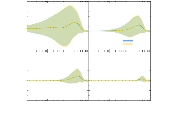
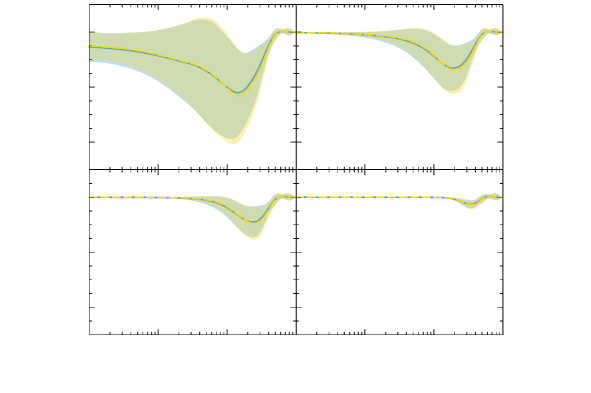
Although the inclusion of WACS data in the analysis of GPDs leads to significant changes in the shapes of extracted polarized valence GPDs at larger values of $-t$, the situation is different for the case of up and down sea quark GPDs $\widetilde{H}^{\bar{u}}$ and $\widetilde{H}^{\bar{d}}$, since their contributions in the theoretical calculations of AFF and WACS cross section are small compared with the valence ones Diehl:2004cx ; Diehl:2013xca . Figure 6 shows the same comparison as Fig. 5 but for the $\widetilde{H}^{\bar{u}}$ (top panel) and $\widetilde{H}^{\bar{d}}$ (bottom panel) GPDs. As can be seen, in this case, there are no considerable differences between the HGG20 and HGG19 GPDs even at larger values of $-t$. This indicates that both AFF and WACS data lead to similar behavior for the sea quark polarized GPDs.

Figure 6: Same as Fig. 5 but for the up and down sea quark GPDs $\widetilde{H}^{\bar{u}}$ (top panel) and $\widetilde{H}^{\bar{d}}$ (bottom panel).

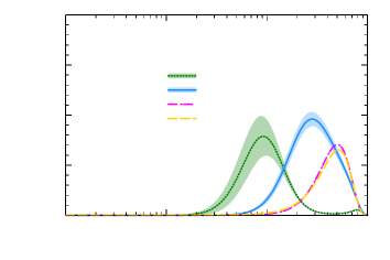
In the Introduction, we compared two sets of polarized GPDs $\widetilde{H}_{v}^{u}$ and $\widetilde{H}_{v}^{d}$ (see Fig. 1) from our previous work Hashamipour:2019pgy (HGG19) which analyzed the AFF data solely and Kroll’s work Kroll:2017hym which considered only the WACS data. We showed that there are considerable differences between these two sets of GPDs at large value of $-t$ (4 GeV²) so that the Kroll’s results are more inclined to larger $x$. Therefore, it is of interest now to compare our new polarized GPDs (HGG20) with the HGG19 and Kroll’s ones since we have extracted them using a simultaneous analysis of AFF and WACS data. Fig. 7 shows such a comparison between the results obtained for the $\widetilde{H}_{v}^{u}$ (top panel) and $\widetilde{H}_{v}^{d}$ (bottom panel) GPDs from four analyses HGG19 (dotted curve), Kroll-I (dashed curve), Kroll-II (dotted-dashed curve), and HGG20 (solid curve) at $t=-4$ GeV². This figure indicates that the simultaneous analysis of AFF and WACS data leads to a significant shift of the valence polarized GPDs to the large $x$ region at larger values of $-t$. Indeed, one can clearly see the better agreement of our results with those of Kroll after the inclusion of the WACS data in the analysis. Kroll did not report uncertainty for his distribution, we guess that his uncertainty should be same order as ours and as a result the uncertainty bands would touch. From the bottom panel of Fig. 7 we infer that the inclusion of the AFF data affects significantly $\widetilde{H}_{v}^{d}$, since both analyses containing these data (HGG19 and HGG20) have a distribution which is greater by an order of magnitude than the Kroll-I and Kroll-II.

Figure 7: A comparison between the results of four analyses HGG19 (dotted curve), Kroll-I (dashed curve), Kroll-II (dotted-dashed curve), and HGG20 (solid curve) for the polarized GPDs $\widetilde{H}_{v}^{u}$ (top panel) and $\widetilde{H}_{v}^{d}$ (bottom panel) at $t=-4$ GeV². See Sec. IV.4 for more information.

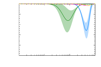
As mentioned in Sec. IV.1, it is also of interest to study the impact of using a more flexible profile function for $\widetilde{H}_{v}^{d}$ by letting $\widetilde{A}_{d_{v}}$ and $\widetilde{B}_{d_{v}}$ be free parameters, leading to symmetrical Ansatzes for $\widetilde{H}_{v}^{u}$ and $\widetilde{H}_{v}^{d}$. By performing a new analysis of the AFF and WACS data using scenario 3 for calculating the WACS cross section, and the CT14 PDFs and NNPDFpol1.1 PPDFs in Ansatzes (20) and (24), respectively, and also adding two free parameters $\widetilde{A}_{d_{v}}$ and $\widetilde{B}_{d_{v}}$ in profile function $\widetilde{f}_{d_{v}}(x)$ of Eq. (IV.1), the optimum values of the fit parameters are obtained as follows,

$$\widetilde{\alpha^{\prime}}_{v}=0.98\pm 0.02,\qquad\mu^{2}=2.22\pm 0.82,$$

$$\widetilde{A}_{u_{v}}=3.79\pm 0.22,\qquad\widetilde{B}_{u_{v}}=-1.82\pm 0.05,$$

$$\widetilde{A}_{d_{v}}=9.85\pm 3.43,\qquad\widetilde{B}_{d_{v}}=-2.48\pm 0.43,$$

and the value of $\chi^{2}/\mathrm{d.o.f.}$ increases by 0.03 (from 4.41 to 4.44), though the value of $\chi^{2}$ itself decreases by about 7 units (from 242.5 to 235.1). Comparing these values with the corresponding ones from Table 4 (see column entitled CT14), one observes that the differences between the $\widetilde{\alpha^{\prime}}_{v}$, $\widetilde{A}_{u_{v}}$, and $\widetilde{B}_{u_{v}}$ parameters are not significant. However, the value of $\mu^{2}$ has increased considerably from 1.48 to 2.22 GeV². By calculating $\widetilde{H}_{v}^{u}(x)$ and $\widetilde{H}^{\bar{q}}(x)$ using the new values obtained for their parameters and comparing them with the previous distributions at typical values of $-t$, we have found that their graphs have not changed significantly by adding two free parameters for $\widetilde{H}_{v}^{d}(x)$. However, their uncertainties have increased, as the numbers reported above for the parameters clearly indicate. It is worth noting that the uncertainties obtained for the two new parameters $\widetilde{A}_{d_{v}}$ and $\widetilde{B}_{d_{v}}$ of $\widetilde{H}_{v}^{d}(x)$ are considerably larger than those of the corresponding parameters of $\widetilde{H}_{v}^{u}(x)$.

Figure 8 shows a comparison between the $\widetilde{H}_{v}^{d}(x)$ obtained from the analysis performed by adding two free parameters $\widetilde{A}_{d_{v}}$ and $\widetilde{B}_{d_{v}}$ in profile function $\widetilde{f}_{d_{v}}(x)$ of Eq. (IV.1) labeled as “HGG20-II” and the corresponding one from the previous analysis (HGG20) at $-t=1$ GeV². As can be seen, there are significant differences between the results of these two analyses. To be more precise, the peak value has decreased by about a factor of two, and its position has shifted from about $x=0.3$ to $x=0.1$. If we superimpose Fig. 8 onto Fig. 7 and compare the trends of changes in the five graphs, we can see that HGG20-II, having equivalent Ansatzes for the up and down valance quarks, is more appropriate. However the increase in the uncertainty is substantial, indicating that the available data is insufficient to fully support this case.

Figure 8: A comparison between the $\widetilde{H}_{v}^{d}(x)$ obtained from two analyses HGG20 (blue solid curve) and HGG20-II (orange dashed curve) at $-t=1$ GeV². See text for details.

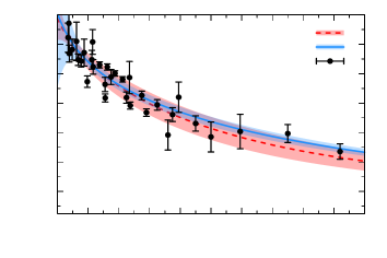
IV.5 Data-theory comparison

Now it is time to compare the theoretical predictions of the AFF and WACS cross section obtained using the final GPDs presented in the previous subsections with the experimental data included in the analysis in order to check the validity of the fit. Figure 9 shows a comparison between the theoretical predictions for the nucleon axial form factor $G_{A}$ with their uncertainties obtained using the HGG20 (blue solid curve) and HGG19 red dashed curve) GPDs and the experimental data included in the analysis (see Sec. III and Table 3). Note again that the HGG20 prediction has been calculated using the polarized GPDs $\widetilde{H}$ obtained from the analysis considering the CT14 as PDFs set and NNPDFpol1.1 as PPDFs set. As can be seen, the agreement between the theory and data has improved in the HGG20 analysis compared to our previous work (HGG19), where we analyzed the AFF data solely. Another point that should be noted is a considerable reduction in the error band of the HGG20 prediction compared to the HGG19, for $x\gtrsim 0.2$, though it is wider for smaller values of $x$.

Figure 9: A comparison between the theoretical predictions of the $G_{A}$ with their uncertainties obtained using the HGG20 (blue solid curve) and HGG19 (red dashed curve) GPDs and the experimental data listed in Table 3.

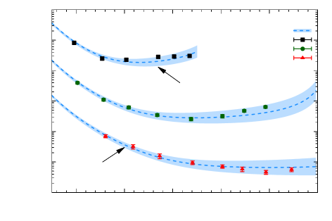
In Fig. 10 we have presented a comparison between the experimental data of the WACS cross section ($d\sigma/dt$) included in the analysis with the related theoretical predictions obtained using our final unpolarized ($H$) and polarized ($\widetilde{H}$) GPDs and considering scenario 3 of Eq. (II.2). The data points belong to three different values of $s$, namely $s=6.79,8.90,$ and 10.92 GeV², which have been shown by the square, circle, and triangle symbols, respectively. The vertical error bars contain both the statistical and systematic uncertainties added in quadrature. It should be noted that in order to better distinguish between the results of these three values of $s$, we have multiplied the experimental data and theoretical predictions of the first and third by a factor of 10 and 1/10, respectively. This figure clearly shows a good agreement between the theoretical predictions and experimental data in the entire interval of $-t$ under consideration, and thus the good quality of the fit. Indeed, almost all data points are within the error band of the theoretical predictions. According to this figure, the reason for the relatively large $\chi^{2}$/$N_{\textrm{pts.}}$ of these data (112/25 for the CT14 analysis in Table 3) is not the poor theoretical description of the data, but it is due to the small values of the experimental uncertainties which appear in the denominator of the expression for $\chi^{2}$.

Figure 10: A comparison between the experimental data of the WACS cross section ($d\sigma/dt$) with the related theoretical predictions obtained using our final GPDs. The data points belong to three different values of $s$, namely $s=6.79,8.90,$ and 10.92 GeV², which have been shown by the square, circle, and triangle symbols, respectively. Multiplication factors indicated are to distinguish the graphs.

IV.6 Proton tomography

As we explained in Sec. II.4, one can associate the physical interpretation of a probability density with the impact parameter dependent PDFs, which are the Fourier transforms of GPDs at zero skewness. In this subsection, we calculate the impact parameter dependent PDFs and present proton tomography in impact parameter space using our final GPDs obtained from the simultaneous analysis of the AFF and WACS data.

In Fig. 11, we have plotted the average shift $s_{q}(x)$ of the distance between struck quark and spectators in a transversely polarized proton for the up (blue solid curve) and down (green dotted-dashed curve) quarks, obtained using Eq. (31). Note that for the case of down quark, since the values of $s$ are negative, we have presented the results as $-s_{d}(x)$ to make the comparison more clear. In fact, the different signs of $s_{u}(x)$ and $s_{d}(x)$ come from the different signs of the anomalous magnetic moments of the up and down quarks Diehl:2004cx . Note that, according to Eqs. (30) and (31), one needs both $H_{v}^{q}$ and $E_{v}^{q}$ GPDs for calculating $s_{q}(x)$. As mentioned before, in our analysis, we have fixed $E_{v}^{q}$ from the analysis of Ref. Diehl:2004cx and just parameterized the $H$ and $\widetilde{H}$ GPDs. Therefore, for calculating $s_{q}(x)$ in Fig. 11, we have used our final result for $H_{v}^{q}$ and the result of Ref. Diehl:2004cx for $E_{v}^{q}$.

Figure 11: Average shift $s_{q}(x)$ of the distance between struck quark and spectators in a polarized proton, defined in Eq. (31), for the up (blue solid curve) and down (green dotted-dashed curve) quarks.

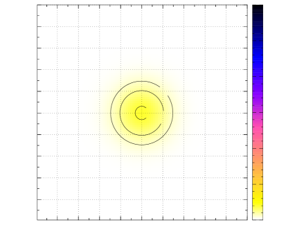
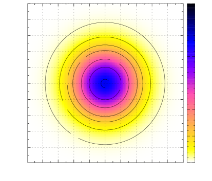
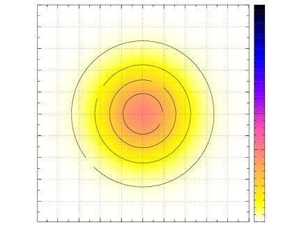
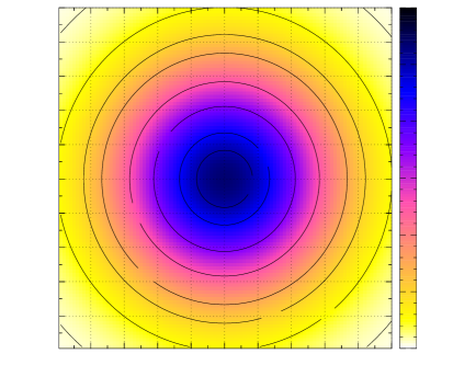
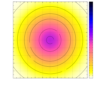
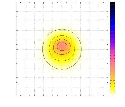
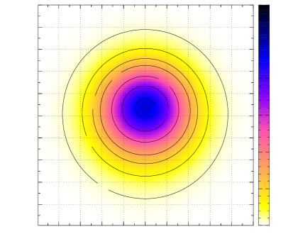
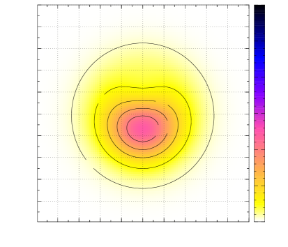
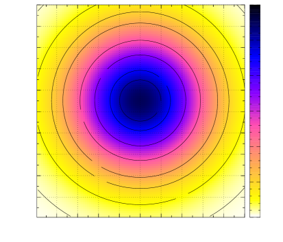
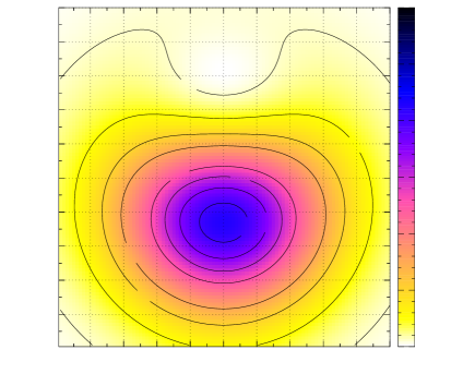
As a further illustration, in Figs. 12 and 13 we have shown our final results for GPDs as tomography plots in impact parameter space for fixed $x$. To be more precise, Fig. 12 displays the results of the unpolarized density $q_{v}(x,\bm{b})$ for the up (left frames) and down (right frames) quarks that have been calculated using Eq. (25) at three fixed values of $x$, namely $x=0.6,0.3,0.05$. Figure 13 shows the corresponding results for the unpolarized density $q_{v}^{X}(x,\bm{b})$ that have been calculated using Eq. (28) for transversely polarized proton. It is obvious from these figures that the displacement of the center of the $q_{v}^{X}(x,\bm{b})$ distribution along the $b^{y}$-axis is different for the up and down quarks. In fact, it is expected from different signs of $s_{u}(x)$ and $s_{d}(x)$ that the center of the $q_{v}^{X}(x,\bm{b})$ density will be shifted toward negative $b^{y}$ for down quarks, whereas it will be shifted toward positive $b^{y}$ for up quarks. It should also be noted that the observed difference between the $q_{v}^{X}(x,\bm{b})$ and $q_{v}(x,\bm{b})$ for down quark at small $x$ compared to the corresponding results for the up quark is due to the fact that the shift $|s_{d}(x)|$ is significantly larger than $s_{u}(x)$ at small values of $x$ (see Fig. 11).

Figure 12: Tomography plots of the unpolarized density $q_{v}(x,\bm{b})$ for the up (left frames) and down (right frames) quarks in the transverse $\bm{b}=(b^{x},b^{y})$ plane at three fixed $x$, namely $x=0.6,0.3,0.05$. The values of $q_{v}(x,\mathbf{b})$ have been shown by color and some guiding contours have been drawn. The unit of $q_{v}(x,\mathbf{b})$ is fm^-2.

Figure 13: Same as Fig. 12 but for the density $q_{v}^{X}(x,\bm{b})$.

V summary and conclusions

It has been well established that the structure of the nucleon, in both the unpolarized and polarized cases, can be investigated in greater detail using GPDs. According to the DFJK model, GPDs can be expressed in terms of PDFs at zero skewness. In this work, considering DFJK model, we have determined both the unpolarized ($H$) and polarized ($\widetilde{H}$) GPDs for quarks at NLO using a simultaneous $\chi^{2}$ analysis of the nucleon AFF and WACS experimental data. It can be considered as a continuation of our previous work Hashamipour:2019pgy where we extracted the polarized GPDs, namely HGG19, through a $\chi^{2}$ analysis of the AFF data solely. The experimental data included in our analysis cover a wide range of the squared transverse momentum $-t$, i.e., $0.025<-t<6.46$ GeV². In order to find the best set of GPDs, we have performed various analyses of the AFF and WACS data using different approaches. In this regard, we first performed a parameterization scan to find the optimum form of profile function Ansatzes for each flavor of $H$ and $\widetilde{H}$ GPDs and reduce the number of free parameters as many as possible. Next, we have considered the three different prescriptions or scenarios for relating the Mandelstam variables at the partonic level to those of the whole process, i.e. at the nucleon level. Then, by performing three separate analyses, we have found the best scenario, namely scenario 3 given by Eq. (II.2), for calculating the WACS cross section theoretically which leads to the lowest $\chi^{2}$ and thus the best agreement between the theoretical predictions and experimental data. Moreover, we have performed various analyses using different sets of PDFs to study the sensitivity of the fit results to the PDFs set that we choose for calculating the GPDs $H$ and the resulting WACS cross section. We have shown that although there are no significant differences between the analyses performed using different sets of PDFs in view of $\chi^{2}$ and parameter values, the extracted GPDs differ as functions of $x$, especially for the case of down valence and sea quark distributions. After finding the optimum form of profile function for each flavor, the best scenario for calculating WACS cross section, and the most compatible PDFs set, we have presented the final results of the extracted GPDs $H$ and $\widetilde{H}$ with their uncertainties, namely HGG20, and have compared them with the corresponding ones obtained from other analyses. We have shown that there is a good agreement between the HGG20 and DFJK05 Diehl:2004cx unpolarized GPDs, even though the latter has used the experimental data of the Dirac and Pauli FFs, while we have used data from the AFF and WACS. Moreover, we have indicated that the WACS data affect the large $-t$ behavior of GPDs more considerably. The main result of the present work is that the simultaneous analysis of AFF and WACS data leads to polarized GPDs which differs substantially as compared to the ones obtained by analyzing each of the AFF and WACS data separately (see Fig. 7). We have compared the theoretical predictions obtained using the final GPDs with the experimental data included in the analysis, and have shown that there is a good agreement in the entire interval of $-t$ under consideration. Finally, by calculating the distribution in the transverse plane of valence quarks, both in an unpolarized and in a transversely polarized proton, we have presented some tomography plots which illustrate the interplay between longitudinal and transverse partonic degrees of freedom in the proton.

References

- (1) J. Pumplin, D. R. Stump, J. Huston, H. L. Lai, P. M. Nadolsky and W. K. Tung, “New generation of parton distributions with uncertainties from global QCD analysis,” JHEP 0207, 012 (2002) [hep-ph/0201195].
- (2) P. Jimenez-Delgado and E. Reya, “Delineating parton distributions and the strong coupling,” Phys. Rev. D 89, no. 7, 074049 (2014) [arXiv:1403.1852 [hep-ph]].
- (3) S. Dulat et al., “New parton distribution functions from a global analysis of quantum chromodynamics,” Phys. Rev. D 93, no. 3, 033006 (2016) [arXiv:1506.07443 [hep-ph]].
- (4) L. A. Harland-Lang, A. D. Martin, P. Motylinski and R. S. Thorne, “Parton distributions in the LHC era: MMHT 2014 PDFs,” Eur. Phys. J. C 75, no. 5, 204 (2015) [arXiv:1412.3989 [hep-ph]].
- (5) R. D. Ball et al. [NNPDF Collaboration], “Parton distributions for the LHC Run II,” JHEP 1504, 040 (2015) [arXiv:1410.8849 [hep-ph]].
- (6) J. Butterworth et al., “PDF4LHC recommendations for LHC Run II,” J. Phys. G 43, 023001 (2016) [arXiv:1510.03865 [hep-ph]].
- (7) R. D. Ball et al. [NNPDF Collaboration], “Parton distributions from high-precision collider data,” Eur. Phys. J. C 77, no. 10, 663 (2017) [arXiv:1706.00428 [hep-ph]].
- (8) S. Alekhin, J. Blümlein, S. Moch and R. Placakyte, “Parton distribution functions, , and heavy-quark masses for LHC Run II,” Phys. Rev. D 96, no. 1, 014011 (2017) [arXiv:1701.05838 [hep-ph]].
- (9) R. Abdul Khalek et al. [NNPDF Collaboration], “A first determination of parton distributions with theoretical uncertainties,” Eur. Phys. J. C , 79:838 (2019) [arXiv:1905.04311 [hep-ph]].
- (10) R. Abdul Khalek et al. [NNPDF Collaboration], “Parton Distributions with Theory Uncertainties: General Formalism and First Phenomenological Studies,” Eur. Phys. J. C 79, no. 11, 931 (2019) [arXiv:1906.10698 [hep-ph]].
- (11) A. V. Radyushkin, “Theory and applications of parton pseudodistributions,” arXiv:1912.04244 [hep-ph].
- (12) D. de Florian, R. Sassot, M. Stratmann and W. Vogelsang, “Extraction of Spin-Dependent Parton Densities and Their Uncertainties,” Phys. Rev. D 80, 034030 (2009) [arXiv:0904.3821 [hep-ph]].
- (13) J. Blumlein and H. Bottcher, “QCD Analysis of Polarized Deep Inelastic Scattering Data,” Nucl. Phys. B 841, 205 (2010) [arXiv:1005.3113 [hep-ph]].
- (14) E. Leader, A. V. Sidorov and D. B. Stamenov, “Determination of Polarized PDFs from a QCD Analysis of Inclusive and Semi-inclusive Deep Inelastic Scattering Data,” Phys. Rev. D 82, 114018 (2010) [arXiv:1010.0574 [hep-ph]].
- (15) D. de Florian, R. Sassot, M. Stratmann and W. Vogelsang, “Evidence for polarization of gluons in the proton,” Phys. Rev. Lett. 113, no. 1, 012001 (2014) [arXiv:1404.4293 [hep-ph]].
- (16) E. R. Nocera et al. [NNPDF Collaboration], “A first unbiased global determination of polarized PDFs and their uncertainties,” Nucl. Phys. B 887, 276 (2014) [arXiv:1406.5539 [hep-ph]].
- (17) P. Jimenez-Delgado et al. [Jefferson Lab Angular Momentum (JAM) Collaboration], “Constraints on spin-dependent parton distributions at large x from global QCD analysis,” Phys. Lett. B 738, 263 (2014) [arXiv:1403.3355 [hep-ph]].
- (18) N. Sato et al. [Jefferson Lab Angular Momentum Collaboration], “Iterative Monte Carlo analysis of spin-dependent parton distributions,” Phys. Rev. D 93, no. 7, 074005 (2016) [arXiv:1601.07782 [hep-ph]].
- (19) F. Taghavi-Shahri, H. Khanpour, S. Atashbar Tehrani and Z. Alizadeh Yazdi, “Next-to-next-to-leading order QCD analysis of spin-dependent parton distribution functions and their uncertainties: Jacobi polynomials approach,” Phys. Rev. D 93, no. 11, 114024 (2016) [arXiv:1603.03157 [hep-ph]].
- (20) H. Khanpour, S. T. Monfared and S. Atashbar Tehrani, “Nucleon spin structure functions at NNLO in the presence of target mass corrections and higher twist effects,” Phys. Rev. D 95, no. 7, 074006 (2017) [arXiv:1703.09209 [hep-ph]].
- (21) J. J. Ethier, N. Sato and W. Melnitchouk, “First simultaneous extraction of spin-dependent parton distributions and fragmentation functions from a global QCD analysis,” Phys. Rev. Lett. 119, no. 13, 132001 (2017) [arXiv:1705.05889 [hep-ph]].
- (22) M. Salajegheh, S. M. Moosavi Nejad, M. Nejad, H. Khanpour and S. Atashbar Tehrani, “Analytical approaches to the determination of spin-dependent parton distribution functions at NNLO approximation,” Phys. Rev. C 97, no. 5, 055201 (2018) [arXiv:1801.04471 [hep-ph]].
- (23) K. Goeke, M. V. Polyakov and M. Vanderhaeghen, “Hard exclusive reactions and the structure of hadrons,” Prog. Part. Nucl. Phys. 47, 401 (2001) [hep-ph/0106012].
- (24) M. Diehl, “Generalized parton distributions,” Phys. Rept. 388, 41 (2003) [hep-ph/0307382].
- (25) M. V. Polyakov, “Generalized parton distributions and strong forces inside nucleons and nuclei,” Phys. Lett. B 555, 57 (2003) [hep-ph/0210165].
- (26) A. Freund, M. McDermott and M. Strikman, “Modeling generalized parton distributions to describe deeply virtual Compton scattering data,” Phys. Rev. D 67, 036001 (2003) [hep-ph/0208160].
- (27) S. Scopetta and V. Vento, “Generalized parton distributions and composite constituent quarks,” Phys. Rev. D 69, 094004 (2004) [hep-ph/0307150].
- (28) A. V. Belitsky and A. V. Radyushkin, “Unraveling hadron structure with generalized parton distributions,” Phys. Rept. 418, 1 (2005) [hep-ph/0504030].
- (29) S. Boffi and B. Pasquini, “Generalized parton distributions and the structure of the nucleon,” Riv. Nuovo Cim. 30, 387 (2007) [arXiv:0711.2625 [hep-ph]].
- (30) V. Guzey and M. V. Polyakov, “Dual parameterization of generalized parton distributions and description of DVCS data,” Eur. Phys. J. C 46, 151 (2006) [hep-ph/0507183].
- (31) V. Guzey and T. Teckentrup, “The Dual parameterization of the proton generalized parton distribution functions H and E and description of the DVCS cross sections and asymmetries,” Phys. Rev. D 74, 054027 (2006) [hep-ph/0607099].
- (32) K. Goeke, V. Guzey and M. Siddikov, “Generalized parton distributions and Deeply Virtual Compton Scattering in Color Glass Condensate model,” Eur. Phys. J. C 56, 203 (2008) [arXiv:0804.4424 [hep-ph]].
- (33) P. Hagler et al. [LHPC Collaboration], “Nucleon Generalized Parton Distributions from Full Lattice QCD,” Phys. Rev. D 77, 094502 (2008) [arXiv:0705.4295 [hep-lat]].
- (34) C. Alexandrou, M. Constantinou, S. Dinter, V. Drach, K. Jansen, C. Kallidonis and G. Koutsou, “Nucleon form factors and moments of generalized parton distributions using twisted mass fermions,” Phys. Rev. D 88, no. 1, 014509 (2013) [arXiv:1303.5979 [hep-lat]].
- (35) K. Kumericki, D. Mueller and K. Passek-Kumericki, “Towards a fitting procedure for deeply virtual Compton scattering at next-to-leading order and beyond,” Nucl. Phys. B 794, 244 (2008) [hep-ph/0703179 [HEP-PH]].
- (36) M. Guidal, H. Moutarde and M. Vanderhaeghen, “Generalized Parton Distributions in the valence region from Deeply Virtual Compton Scattering,” Rept. Prog. Phys. 76, 066202 (2013) [arXiv:1303.6600 [hep-ph]].
- (37) K. Kumericki, S. Liuti and H. Moutarde, “GPD phenomenology and DVCS fitting : Entering the high-precision era,” Eur. Phys. J. A 52, no. 6, 157 (2016) [arXiv:1602.02763 [hep-ph]].
- (38) H. Khanpour, M. Goharipour and V. Guzey, “Effects of next-to-leading order DGLAP evolution on generalized parton distributions of the proton and deeply virtual Compton scattering at high energy,” Eur. Phys. J. C 78, no. 1, 7 (2018) [arXiv:1708.05740 [hep-ph]].
- (39) P. Kroll, “The GPD and spin correlations in wide-angle Compton scattering,” Eur. Phys. J. A 53, no. 6, 130 (2017) [arXiv:1703.05000 [hep-ph]].
- (40) N. Kaur, N. Kumar, C. Mondal and H. Dahiya, “Generalized Parton Distributions of Pion for Non-Zero Skewness in AdS/QCD,” Nucl. Phys. B 934, 80 (2018) [arXiv:1807.01076 [hep-ph]].
- (41) H. Moutarde, P. Sznajder and J. Wagner, “Border and skewness functions from a leading order fit to DVCS data,” Eur. Phys. J. C 78, no. 11, 890 (2018) [arXiv:1807.07620 [hep-ph]].
- (42) B. D. Sun and Y. B. Dong, “Polarized generalized parton distributions and structure functions of the meson,” Phys. Rev. D 99, no. 1, 016023 (2019) [arXiv:1811.00666 [hep-ph]].
- (43) G. F. de Teramond et al. [HLFHS Collaboration], “Universality of Generalized Parton Distributions in Light-Front Holographic QCD,” Phys. Rev. Lett. 120, no. 18, 182001 (2018) [arXiv:1801.09154 [hep-ph]].
- (44) G. Duplančić, K. Passek-Kumerički, B. Pire, L. Szymanowski and S. Wallon, “Probing axial quark generalized parton distributions through exclusive photoproduction of a pair with a large invariant mass,” JHEP 1811, 179 (2018) [arXiv:1809.08104 [hep-ph]].
- (45) M. Siddikov and I. Schmidt, “Generalized Parton Distributions from charged current meson production,” Phys. Rev. D 99, no. 11, 116005 (2019) [arXiv:1904.04252 [hep-ph]].
- (46) B. Kriesten, S. Liuti, L. Calero-Diaz, D. Keller, A. Meyer, G. R. Goldstein and J. Osvaldo Gonzalez-Hernandez, “Extraction of Generalized Parton Distribution Observables from Deeply Virtual Electron Proton Scattering Experiments,” Phys. Rev. D 101, no.5, 054021 (2020) [arXiv:1903.05742 [hep-ph]].
- (47) H. Hashamipour, M. Goharipour and S. S. Gousheh, “Nucleon axial form factor from generalized parton distributions,” Phys. Rev. D 100, no. 1, 016001 (2019) [arXiv:1903.05542 [hep-ph]].
- (48) P. Kroll, “The role of the GPD E in the determination of the parton angular momenta,” arXiv:2001.01919 [hep-ph].
- (49) X. D. Ji and J. Osborne, “One loop corrections and all order factorization in deeply virtual Compton scattering,” Phys. Rev. D 58, 094018 (1998) [hep-ph/9801260].
- (50) J. C. Collins and A. Freund, “Proof of factorization for deeply virtual Compton scattering in QCD,” Phys. Rev. D 59, 074009 (1999) [hep-ph/9801262].
- (51) P. Kroll, M. Schurmann and P. A. M. Guichon, “Virtual Compton scattering off protons at moderately large momentum transfer,” Nucl. Phys. A 598, 435 (1996) [hep-ph/9507298].
- (52) X. D. Ji, “Deeply virtual Compton scattering,” Phys. Rev. D 55, 7114 (1997) [hep-ph/9609381].
- (53) P. A. M. Guichon and M. Vanderhaeghen, “Virtual Compton scattering off the nucleon,” Prog. Part. Nucl. Phys. 41, 125 (1998) [hep-ph/9806305].
- (54) A. V. Belitsky, D. Mueller and A. Kirchner, “Theory of deeply virtual Compton scattering on the nucleon,” Nucl. Phys. B 629, 323 (2002) [hep-ph/0112108].
- (55) A. V. Belitsky, D. Müller and Y. Ji, “Compton scattering: from deeply virtual to quasi-real,” Nucl. Phys. B 878, 214 (2014) [arXiv:1212.6674 [hep-ph]].
- (56) M. Benali et al., “Deeply virtual Compton scattering off the neutron,” Nature Phys. 16, no. 2, 191 (2020).
- (57) D. Müller, D. Robaschik, B. Geyer, F.-M. Dittes and J. Hořejši, “Wave functions, evolution equations and evolution kernels from light ray operators of QCD,” Fortsch. Phys. 42, 101 (1994) [hep-ph/9812448].
- (58) J. C. Collins, L. Frankfurt and M. Strikman, “Factorization for hard exclusive electroproduction of mesons in QCD,” Phys. Rev. D 56, 2982 (1997) [hep-ph/9611433].
- (59) L. Favart, M. Guidal, T. Horn and P. Kroll, “Deeply Virtual Meson Production on the nucleon,” Eur. Phys. J. A 52, no. 6, 158 (2016) [arXiv:1511.04535 [hep-ph]].
- (60) W. Brooks, I. Schmidt and M. Siddikov, “Deeply virtual meson production on neutrons,” Phys. Rev. D 98, no. 11, 116006 (2018) [arXiv:1810.08077 [hep-ph]].
- (61) E. R. Berger, M. Diehl and B. Pire, “Time - like Compton scattering: Exclusive photoproduction of lepton pairs,” Eur. Phys. J. C 23, 675 (2002) [hep-ph/0110062].
- (62) H. Moutarde, B. Pire, F. Sabatie, L. Szymanowski and J. Wagner, “Timelike and spacelike deeply virtual Compton scattering at next-to-leading order,” Phys. Rev. D 87, no. 5, 054029 (2013) [arXiv:1301.3819 [hep-ph]].
- (63) M. Boër, M. Guidal and M. Vanderhaeghen, “Timelike Compton scattering off the proton and generalized parton distributions,” Eur. Phys. J. A 51, no. 8, 103 (2015).
- (64) M. Diehl, T. Gousset and B. Pire, “Exclusive electroproduction of vector mesons and transversity distributions,” Phys. Rev. D 59, 034023 (1999) [hep-ph/9808479].
- (65) L. Mankiewicz and G. Piller, “Comments on exclusive electroproduction of transversely polarized vector mesons,” Phys. Rev. D 61, 074013 (2000) [hep-ph/9905287].
- (66) I. V. Anikin, D. Y. Ivanov, B. Pire, L. Szymanowski and S. Wallon, “QCD factorization of exclusive processes beyond leading twist: gamma*T —¿ rho(T) impact factor with twist three accuracy,” Nucl. Phys. B 828, 1 (2010) [arXiv:0909.4090 [hep-ph]].
- (67) D. Y. Ivanov, A. Schafer, L. Szymanowski and G. Krasnikov, “Exclusive photoproduction of a heavy vector meson in QCD,” Eur. Phys. J. C 34, no. 3, 297 (2004) Erratum: [Eur. Phys. J. C 75, no. 2, 75 (2015)] [hep-ph/0401131].
- (68) M. Guidal and M. Vanderhaeghen, “Double deeply virtual Compton scattering off the nucleon,” Phys. Rev. Lett. 90, 012001 (2003) [hep-ph/0208275].
- (69) A. V. Belitsky and D. Mueller, “Exclusive electroproduction of lepton pairs as a probe of nucleon structure,” Phys. Rev. Lett. 90, 022001 (2003) [hep-ph/0210313].
- (70) D. Mueller, B. Pire, L. Szymanowski and J. Wagner, “On timelike and spacelike hard exclusive reactions,” Phys. Rev. D 86, 031502 (2012) [arXiv:1203.4392 [hep-ph]].
- (71) T. Sawada, W. C. Chang, S. Kumano, J. C. Peng, S. Sawada and K. Tanaka, “Accessing proton generalized parton distributions and pion distribution amplitudes with the exclusive pion-induced Drell-Yan process at J-PARC,” Phys. Rev. D 93, no. 11, 114034 (2016) [arXiv:1605.00364 [nucl-ex]].
- (72) R. Boussarie, B. Pire, L. Szymanowski and S. Wallon, “Exclusive photoproduction of a pair with a large invariant mass,” JHEP 1702, 054 (2017) Erratum: [JHEP 1810, 029 (2018)] [arXiv:1609.03830 [hep-ph]].
- (73) A. Pedrak, B. Pire, L. Szymanowski and J. Wagner, “Hard photoproduction of a diphoton with a large invariant mass,” Phys. Rev. D 96, no. 7, 074008 (2017) Erratum: [Phys. Rev. D 100, no. 3, 039901 (2019)] [arXiv:1708.01043 [hep-ph]].
- (74) B. Z. Kopeliovich, I. Schmidt and M. Siddikov, “Flavor structure of generalized parton distributions from neutrino experiments,” Phys. Rev. D 86, 113018 (2012) [arXiv:1210.4825 [hep-ph]].
- (75) B. Pire, L. Szymanowski and J. Wagner, “Hard exclusive neutrino production of a light meson,” Phys. Rev. D 95, no. 11, 114029 (2017) [arXiv:1705.11088 [hep-ph]].
- (76) B. Pire, L. Szymanowski and J. Wagner, “Exclusive neutrino-production of a charmed meson,” Phys. Rev. D 95, no. 9, 094001 (2017) [arXiv:1702.00316 [hep-ph]].
- (77) S. Kofler, P. Kroll and W. Schweiger, “ within the Generalized Parton Picture,” Phys. Rev. D 91, 054027 (2015) [arXiv:1412.5367 [hep-ph]].
- (78) A. Accardi et al., “Electron Ion Collider: The Next QCD Frontier : Understanding the glue that binds us all,” Eur. Phys. J. A 52, no. 9, 268 (2016) [arXiv:1212.1701 [nucl-ex]].
- (79) B. Pasquini, M. Pincetti and S. Boffi, “Chiral-odd generalized parton distributions in constituent quark models,” Phys. Rev. D 72, 094029 (2005) [hep-ph/0510376].
- (80) B. Pasquini and S. Boffi, “Virtual meson cloud of the nucleon and generalized parton distributions,” Phys. Rev. D 73, 094001 (2006) [hep-ph/0601177].
- (81) H. Dahiya and A. Mukherjee, “Chiral Odd Generalized Parton Distributions in Impact Parameter Space,” Phys. Rev. D 77, 045032 (2008) [arXiv:0711.1566 [hep-ph]].
- (82) T. Frederico, E. Pace, B. Pasquini and G. Salme, “Pion Generalized Parton Distributions with covariant and Light-front constituent quark models,” Phys. Rev. D 80, 054021 (2009) [arXiv:0907.5566 [hep-ph]].
- (83) A. Mukherjee, S. Nair and V. Kumar Ojha, “Generalized Parton Distributions of the Photon with Helicity Flip,” Phys. Lett. B 721, 284 (2013) [arXiv:1301.6895 [hep-ph]].
- (84) T. Maji, C. Mondal, D. Chakrabarti and O. V. Teryaev, “Relating transverse structure of various parton distributions,” JHEP 1601, 165 (2016) [arXiv:1506.04560 [hep-ph]].
- (85) G. R. Goldstein, J. O. Hernandez and S. Liuti, “Flexible parametrization of Generalized Parton Distributions from Deeply Virtual Compton Scattering Observables,” Phys. Rev. D 84, 034007 (2011) [arXiv:1012.3776 [hep-ph]].
- (86) G. R. Goldstein, J. O. Gonzalez Hernandez and S. Liuti, “Flexible parametrization of Generalized Parton Distributions: The Chiral-Odd Sector,” Phys. Rev. D 91, no. 11, 114013 (2015) [arXiv:1311.0483 [hep-ph]].
- (87) N. Sharma, “Momentum transfer dependence of generalized parton distributions,” Eur. Phys. J. A 52, no. 11, 338 (2016) [arXiv:1610.07745 [hep-ph]].
- (88) V. Kubarovsky [CLAS Collaboration], “Deeply virtual exclusive reactions with CLAS,” Nucl. Phys. Proc. Suppl. 219-220, 118 (2011).
- (89) W. Armstrong et al., “Partonic Structure of Light Nuclei,” arXiv:1708.00888 [nucl-ex].
- (90) N. d’Hose, E. Burtin, P. A. M. Guichon and J. Marroncle, “Feasibility study of deeply virtual Compton scattering using COMPASS at CERN,” Eur. Phys. J. A 19S1, 47 (2004).
- (91) L. Silva, “Experimental Program of the Future COMPASS-II Experiment at CERN,” Few Body Syst. 54, no. 7-10, 1075 (2013).
- (92) O. Kouznetsov [COMPASS Collaboration], “GPD study programme of COMPASS at CERN,” Nucl. Part. Phys. Proc. 270-272, 36 (2016).
- (93) P. Kroll, “The exclusive Drell-Yan process and deeply virtual pion production,” JPS Conf. Proc. 13, 010014 (2017) [arXiv:1611.01623 [hep-ph]].
- (94) J. L. Abelleira Fernandez et al. [LHeC Study Group], “A Large Hadron Electron Collider at CERN: Report on the Physics and Design Concepts for Machine and Detector,” J. Phys. G 39, 075001 (2012) [arXiv:1206.2913 [physics.acc-ph]].
- (95) M. Diehl, T. Feldmann, R. Jakob and P. Kroll, “Generalized parton distributions from nucleon form-factor data,” Eur. Phys. J. C 39, 1 (2005) [hep-ph/0408173].
- (96) M. Diehl, T. Feldmann and P. Kroll, “Form factors and other measures of strangeness in the nucleon,” Phys. Rev. D 77, 033006 (2008) [arXiv:0711.4304 [hep-ph]].
- (97) M. Diehl and P. Kroll, “Nucleon form factors, generalized parton distributions and quark angular momentum,” Eur. Phys. J. C 73, no. 4, 2397 (2013) [arXiv:1302.4604 [hep-ph]].
- (98) X. D. Ji, “Gauge-Invariant Decomposition of Nucleon Spin,” Phys. Rev. Lett. 78, 610 (1997) [hep-ph/9603249].
- (99) C. Mondal, S. Xu, J. Lan, X. Zhao, Y. Li, D. Chakrabarti and J. P. Vary, “Proton structure from a light-front Hamiltonian,” arXiv:1911.10913 [hep-ph].
- (100) V. Bernard, L. Elouadrhiri and U. G. Meissner, “Axial structure of the nucleon: Topical Review,” J. Phys. G 28, R1 (2002) [hep-ph/0107088].
- (101) M. R. Schindler and S. Scherer, “Nucleon Form Factors of the Isovector Axial-Vector Current: Situation of Experiments and Theory,” Eur. Phys. J. A 32, no. 4, 429 (2007) [hep-ph/0608325].
- (102) H. W. Huang, P. Kroll and T. Morii, “Perturbative and nonperturbative QCD corrections to wide angle Compton scattering,” Eur. Phys. J. C 23, 301 (2002) Erratum: [Eur. Phys. J. C 31, 279 (2003)] [hep-ph/0110208].
- (103) M. Diehl, T. Feldmann, H. W. Huang and P. Kroll, “Proton mass effects in wide angle Compton scattering,” Phys. Rev. D 67, 037502 (2003) [hep-ph/0212138].
- (104) A. V. Radyushkin, “Nonforward parton distributions,” Phys. Rev. D 56, 5524 (1997) [hep-ph/9704207].
- (105) S. V. Goloskokov and P. Kroll, “Transversity in hard exclusive electroproduction of pseudoscalar mesons,” Eur. Phys. J. A 47, 112 (2011) [arXiv:1106.4897 [hep-ph]].
- (106) M. Burkardt, “Impact parameter dependent parton distributions and off forward parton distributions for zeta ,” Phys. Rev. D 62, 071503 (2000) Erratum: [Phys. Rev. D 66, 119903 (2002)] [hep-ph/0005108].
- (107) M. Burkardt, “Impact parameter space interpretation for generalized parton distributions,” Int. J. Mod. Phys. A 18, 173 (2003) [hep-ph/0207047].
- (108) A. V. Belitsky, X. d. Ji and F. Yuan, “Quark imaging in the proton via quantum phase space distributions,” Phys. Rev. D 69, 074014 (2004) [hep-ph/0307383].
- (109) M. Burkardt, “Some inequalities for the generalized parton distribution E (x,0,t),” Phys. Lett. B 582, 151 (2004) [hep-ph/0309116].
- (110) A. V. Butkevich and D. Perevalov, “Determination of the Axial Nucleon Form Factor from the MiniBooNE Data,” Phys. Rev. D 89, no. 5, 053014 (2014) [arXiv:1311.3754 [hep-ph]].
- (111) A. Danagoulian et al. [Hall A Collaboration], “Compton scattering cross-section on the proton at high momentum transfer,” Phys. Rev. Lett. 98, 152001 (2007) [nucl-ex/0701068 [NUCL-EX]].
- (112) E. Amaldi, B. Borgia, P. Pistilli, M. Balla, G. V. Di Giorgio, A. Giazotto, S. Serbassi and G. Stoppini, “On pion electroproduction at 5 fm-squared near threshold,” Nuovo Cim. A 65, 377 (1970).
- (113) E. Amaldi, M. Benevantano, B. Borgia, F. De Notaristefani, A. Frondaroli, P. Pistilli, I. Sestili and M. Severi, “Axial-vector form-factor of the nucleon from a coincidence experiment on electroproduction at threshold,” Phys. Lett. 41B, 216 (1972).
- (114) P. Brauel et al., “ electroproduction on hydrogen near threshold at four-momentum transfers of 0.2, 0.4 and 0.6 GeV2,” Phys. Lett. 45B, 389 (1973).
- (115) A. Del Guerra, A. Giazotto, M. A. Giorgi, A. Stefanini, D. R. Botterill, H. E. Montgomery, P. R. Norton and G. Matone, “Threshold electroproduction at high momentum transfer: a determination of the nucleon axial vector form-factor,” Nucl. Phys. B 107, 65 (1976).
- (116) A. Del Guerra, A. Giazotto, M. A. Giorgi, A. Stefanini, D. R. Botterill, D. W. Braben, D. Clarke and P. R. Norton, “Measurements of Threshold pi+ Electroproduction at Low Momentum Transfer,” Nucl. Phys. B 99, 253 (1975).
- (117) A. S. Esaulov, A. M. Pilipenko and Y. I. Titov, “Longitudinal and Transverse Contributions to the Threshold Cross-Section Slope of Single Pion Electroproduction by a Proton,” Nucl. Phys. B 136, 511 (1978).
- (118) E. D. Bloom et al., “Measurements Of Inelastic Electron Scattering Cross-sections Near One Pion Threshold,” Phys. Rev. Lett. 30, 1186 (1973).
- (119) P. Joos et al., “Determination of the Nucleon Axial Vector Form-Factor from pi Delta Electroproduction Near Threshold,” Phys. Lett. 62B, 230 (1976).
- (120) S. Choi et al., “Axial and pseudoscalar nucleon form-factors from low-energy pion electroproduction,” Phys. Rev. Lett. 71, 3927 (1993).
- (121) S. Choi, ”Etude experimentale et theorique de l’electroproduction de pions pres du seuil mesure des facteurs de forme axial et pseudo-scalaire,” These No. 2643, Universite Paris XI Orsay, Paris. (1993).
- (122) M. Tanabashi et al., “Review of Particle Physics,” Phys. Rev. D 98, no. 3, 030001 (2018).
- (123) F. D. Aaron et al. [H1 and ZEUS Collaborations], “Combined Measurement and QCD Analysis of the Inclusive e+- p Scattering Cross Sections at HERA,” JHEP 1001, 109 (2010) [arXiv:0911.0884 [hep-ex]].
- (124) F. James and M. Roos, “Minuit: A System for Function Minimization and Analysis of the Parameter Errors and Correlations,” Comput. Phys. Commun. 10, 343 (1975); F. James, “MINUIT Function Minimization and Error Analysis: Reference Manual Version 94.1,” CERN-D-506, CERN-D506.
- (125) A. Buckley, J. Ferrando, S. Lloyd, K. Nordström, B. Page, M. Rüfenacht, M. Schönherr and G. Watt, “LHAPDF6: parton density access in the LHC precision era,” Eur. Phys. J. C 75, 132 (2015) [arXiv:1412.7420 [hep-ph]].