Constraining nuclear matter parameters from correlation systematics: a mean-field perspective

Abstract

The nuclear matter parameters define the nuclear equation of state (EoS), they appear as coefficients of expansion around the saturation density of symmetric and asymmetric nuclear matter. We review their correlations with several properties of finite nuclei and of neutron stars within mean-field frameworks. The lower order nuclear matter parameters such as the binding energy per nucleon, incompressibility and the symmetry energy coefficients are found to be constrained in narrow limits through their strong ties with selective properties of finite nuclei. From the correlations of nuclear matter parameters with neutron star observables, we further review how precision knowledge of the radii and tidal deformability of neutron stars in the mass range $1-2M_{\odot}$ may help cast them in narrower bounds. The higher order parameters such as the density slope and the curvature of the symmetry energy or the skewness of the symmetric nuclear matter EoS are, however, plagued with larger uncertainty. From inter-correlation of these higher order nuclear matter parameters with lower order ones, we explore how they can be brought to more harmonious bounds.

1 Introduction

Precise determination of the equation of state (EoS) of nuclear matter is one of the major goals in nuclear physics. Relying on a realistic nucleonic interaction, in a microscopic framework, the energy density $\mathcal{E}$ of the system (a finite nucleus or a macroscopic nuclear system) is computed; the parameters of the interaction or of the energy density functional (EDF) are tuned so that the predicted observables calculated with the EDF match with the experimental data. In a broad sweep, the EoS or the EDF then entails knowledge of the diverse nuclear matter parameters that define infinite nuclear matter: its saturation density $\rho_{0}$, the energy per nucleon $e(\rho_{0})$, the incompressibility $K(\rho_{0})$, the symmetry energy coefficient $C_{2}(\rho_{0})$ and their density derivatives of different orders. These nuclear matter parameters enter into the EoS as Taylor expansion coefficients around the saturation density; when precisely determined they stand out as irreducible elements of physical reality as they have the mark of defining a model-independent nuclear EoS.

Not all of the nuclear matter parameters are known in very good bounds. The profusion of data on the masses of atomic nuclei has kept the uncertainties in the values of $\rho_{0}$ and $e(\rho_{0})$ quite small Myers1969 ; Myers1980 ; Moeller2012 . Correlation systematics has proved to be a useful tool in arriving at values of many others. For example, the centroid energy $E_{\scriptsize{GMR}}$ of the isoscalar giant monopole resonance (ISGMR) is a measure of $K(\rho_{0})(=K_{0}=9\rho_{0}^{2}\frac{\partial^{2}e}{\partial\rho^{2}}|_{\rho_{0}}$). The correlation diagram drawn between the predicted ISGMR energies for a heavy nucleus like ²⁰⁸Pb with different EDFs against the related nuclear matter parameter $K_{0}$ pertaining to the EDFs has proved to be an effective method of projecting its value Blaizot1980 at saturation density. Noticing the recently found remarkable soft nuclear matter compression from the ISGMR data in Sn and Cd isotopes Lui2004 ; Li2007 ; Garg2007 ; Li2010 ; Patel2012 , questions are asked Khan2010 ; Khan2012 ; Khan2013 on whether ISGMR energy is a reflection of compression at saturation density or whether $E_{\scriptsize{GMR}}$ is related to the nuclear matter incompressibility averaged over the whole density range within the nucleus. The correlation systematics was, however, not severely called into question. In several non-relativistic and relativistic EDFs, the ISGMR energy $E_{\scriptsize{GMR}}$ was found to be well correlated to $M(\rho_{c}))$, the density derivative of $K(\rho)~{}[M(\rho_{c})=3\rho_{c}K^{\prime}(\rho_{c})]$ at a crossing density $\rho_{c}$ that is close to the average density in a nucleus Khan2012 . A subtle correlation analysis at the end then leads to a value of $K_{0}$ De2015 , $M_{c}$ and also to $K_{c}$, the incompressibility at $\rho_{c}$ Khan2012 .

There is a cultivated focus in recent times in tightening the bounds on the values of the isovector nuclear matter parameters, namely, the symmetry energy $C_{2}^{0}(\equiv C_{2}(\rho_{0}))$ , its density derivative $L_{0}(\equiv L(\rho_{0}))$, the symmetry incompressibility $K_{\rm sym}^{0}(\equiv K_{\rm sym}(\rho_{0}))$ etc RocaMaza2018 . They have a fundamental role in deciding pressures in neutron-rich matter; they determine the nuclear masses, the neutron-skin thickness and the size and structure of neutron stars. From a Bethe-Weizacker type of expansion of the nuclear binding energy in powers of the mass number $A$, the symmetry energy $C_{2}^{0}$ is well obtained Myers1969 ; Moeller2012 ; the exhibited compact correlation of the double differences of the ’experimental symmetry energies’ of four neighboring nuclei with the nuclear mass number $A$ yields Jiang2012 , however, the value of the volume and surface symmetry energies at $\rho_{0}$ with much less uncertainty. No less important is the strong correlation of the value of the centroid of the isovector giant dipole resonance (IVGDR) energy in spherical nuclei with the symmetry energy $C_{2}(\rho)$ Trippa2008 at $\rho\sim 0.1$fm ^-3 found in Skyrme EDFs in imposing a quantitative constraint on the symmetry energy at a sub-saturation density. The value ($C_{2}(\rho\sim 0.1)\approx 23.3\pm 0.8$ MeV) is in extremely good agreement with that found from analysis of experimental isoscalar and isovector giant quadrupole resonances of the nucleus ²⁰⁸Pb RocaMaza2013 .

Systematics in relativistic and non-relativistic models have revealed that there is a strong correlation between the density derivative of symmetry energy $L_{0}$ with the neutron-skin thickness $\Delta r_{np}$ [$=(R_{n}-R_{p})$, $R_{n}$ and $R_{p}$ are the neutron and proton root mean squared radius (rms) ] of a heavy nucleus like ²⁰⁸Pb Brown2000 ; Typel2001 ; Centelles2009 . Analyzing the correlation systematics of nuclear isospin with neutron-skin thickness for a series of nuclei in the ambit of the droplet model, the Barcelona group Centelles2009 ; Warda2009 predicted $L_{0}$ in a comparatively narrow window, but it suffers from the unavoidable strong interaction-related uncertainties in the neutron-skin thickness derived from anti-protonic atom experiments. Finding a model-independent precise value of the neutron-skin thickness is a major challenge still not quite accomplished Abrahamyan2012 , so the converse route of finding $L_{0}$ and then predicting $\Delta r_{np}$ from correlation systematics has been taken by many. The often shifting values of $L_{0}$ obtained from different observables like pygmy dipole resonance Carbone2010 , isovector giant dipole resonance Trippa2008 , nucleonic emission ratios Famiano2006 , nuclear masses Moeller2012 ; Agrawal2012 ; Agrawal2013 or even astrophysical inputs of neutron star radii Steiner2012 render $L_{0}$ and thus $\Delta r_{np}$ still somewhat uncertain. Of late, co-variance analysis with masses of selective highly asymmetric nuclei Mondal2015 and experimental data on collective isovector excitations in nuclei Paar2014 tend to constrain $L_{0}$ tightly, the constraint, however, depends much on the precision of the relevant experimental data.

The multitude of EDFs are rooted to various sets of selective experimental data that may have occasional overlaps. It is therefore not surprising that the bulk nuclear matter parameters (tied to the various parameters in the EDFs) may be intercorrelated and so the nuclear observables display built-in correlations with the nuclear matter parameters pertaining to the concerned EDFs. As examples, further to those mentioned earlier, the core-crust transition density $\rho_{t}$ in neutron star is found to be correlated Horowitz2001 to the neutron-skin $\Delta r_{np}$ in the nucleus ²⁰⁸Pb, $\rho_{t}$ is also seen to be correlated with the symmetry density derivative $L_{0}$ Horowitz2001 ; Ducoin2011 , $\Delta r_{np}$ has a correlation with the product of nuclear dipole polarizability $\alpha_{D}$ with the symmetry energy $C_{2}^{0}$ RocaMaza2015 . Knowledge of a better known entity then throws light on the one lesser known, this is the kernel of the correlation systematics.

The observable properties of neutron stars offer fresh grounds for exploring the nuclear matter EoS on a large density plane, spanning a few times the nuclear saturation density. Behind the solid crust of $\sim 1$ km thickness lies the central homogeneous liquid core, its density increases as one approaches the center. The outer crust is inhomogeneous with neutron-rich nucleons and degenerate electrons. The inner crust, loosely speaking, starts when with increasing density and pressure, neutronization sets in leading to the existence of a neutron ocean with inhomogeneous nucleonic clusters and electrons. The structure of the inner crust is modeled as a lattice in a body centered cubic formation with the electron gas circulating throughout the structure Teukolsky1983 , the free neutrons are assumed to have no effect. However, if the interactions between the neutrons and the lattice are accounted for, a rethink on the structure of the crust and its response to perturbations may be needed Kobyakov2014 . The density at which neutrons drip off from nuclei is rather well known, but the transition density at the inner edge separating the solid crust from the liquid core is still not well settled. The bottom layer of the inner crust consists mostly of exotic nuclear structures collectively known as nuclear pasta Lorenz1993 ; Berry2016 . The transition density offers important insights into the origin of pulsar glitches from its relation to the crustal fraction of the moment of inertia of a neutron star Madhuri2017 with additional information on the gravitational wave radiation GuerraChaves2019 by the neutron star when subjected to a very intense gravitational field.

In this article, we do not deal with the EoS of the neutron star crust, it is assumed to be known Baym1971 , we rather focus on the nuclear matter EoS for the homogeneous core region, from around the saturation density $\rho_{0}$ to the central density of around $\sim 5-6\rho_{0}$, and on the specifics of the nuclear matter parameters that describe them. The analysis of directed and elliptic flow Danielewicz2002 and kaon production Fuchs2006 ; Fantina2014 from heavy ion collisions (HIC) has helped understand the nuclear matter EoS at supra-normal densities. Recently, the detection of gravitational waves from the GW170817 binary neutron star merger Abbott2017 has added much impetus to effectively map the EoS at densities relevant to neutron stars.

Microscopic analysis of different kinds of laboratory data, on the other hand, have probed the nuclear matter EoS at around the saturation density with different levels of satisfaction. Attempts have been made to find a link of these two Malik2018 ; Malik2019 ; Tsang2019 through the nuclear matter parameters , the common denominators appearing as Taylor expansion coefficients in the nuclear matter EoS. Scanning the multitude of terrestrial and astronomical data, coherent systematics have been followed to arrive at their values as best as possible, we aim to describe part of it in this article.

An alternate route, based on ab-initio models (for a brief review, see Ekstroem2019 ) aims at analyzing the properties of finite nuclei and of infinite nuclear matter on a more fundamental level. With a multitude of theoretical descriptions of the interaction between nucleons at various levels of phenomenology Machleidt2001 ; Entem2003 ; Kolck1999 ; Epelbaum2009 ; Machleidt2011 , significant efforts have been employed in solving the many-body Schrödinger equation Lee2009 ; Barrett2013 ; Carbone2013 ; Hagen2014 with as few uncontrolled approximations as possible. The curse of dimensionality in solving the complex many-body problem along with the somewhat hazy knowledge of the nucleonic interaction has limited their predictive power upto only light nuclei and upto density close to saturation density and somewhat beyond Hergert2016 ; Morris2018 ; Holt2019 ; Sammarruca2015 , that too with a precision that may be insufficient. A complementary approach was recently proposed aimed explicitly in bridging the ab-initio methods with an ab-initio equivalent Skyrme EDF Salvioni2020 . This was found to describe properties of nuclei and nuclear matter poorly. Though fundamental, we do not explore the quantification of the nuclear matter parameters in the framework of ab-initio models, but settle on the nuclear matter EoS based on the present broad knowledge of the effective nucleon-nucleon interaction aided by a mean-field perspective.

2 Theoretical Inputs

The energy per nucleon of asymmetric homogeneous nuclear matter at density $\rho$ can be written as,

$$e(\rho,\delta)=e(\rho,\delta=0)+C_{2}(\rho)\delta^{2}+C_{4}(\rho)\delta^{4}+\cdots,$$ (1)

where $\delta=(\rho_{n}-\rho_{p})/\rho$ is the isospin asymmetry of the system. The first term on the right hand side (r.h.s) of Eq. (1) is the energy corresponding to symmetric nuclear matter (SNM), the other terms are the asymmetry contributions. The coefficients $C_{n}(\rho)$ are collectively called the symmetry coefficients. For nearly all energy density functionals, it is found that the parabolic approximation (terms upto $C_{2}$ in Eq. (1)) is quite reasonable for densities upto $\sim 1.5\rho_{0}$ Chen2009 ; Constantinou2014 ; Vidana2002 ; GonzalezBoquera2017 . Around the saturation density $\rho_{0}$, the SNM component $e(\rho,\delta=0)$ can be expanded as,

$$e(\rho,\delta=0)=e_{0}+\frac{1}{2}K_{0}\epsilon^{2}+\frac{1}{6}Q_{0}\epsilon^{3}+\frac{1}{24}Z_{0}\epsilon^{4}+\cdots,$$ (2)

where $e_{0}=e(\rho_{0},\delta=0)$, $\epsilon=(\rho-\rho_{0})/3\rho_{0}$, $K_{0}$ $(=9\rho_{0}^{2}\frac{\partial^{2}e}{\partial\rho^{2}}|_{\rho_{0}})$ is the isoscalar incompressibility, $Q_{0}(=27\rho_{0}^{3}\frac{\partial^{3}e}{\partial\rho^{3}}|_{\rho_{0}})$ the skewness parameter etc. The parameter $Q_{0}$ is related to the density derivative of the nuclear matter incompressibility $(M=3\rho\frac{dK}{d\rho})$ at $\rho_{0}$, $M_{0}=12K_{0}+Q_{0}$. The symmetry coefficient $C_{2}(\rho)$ can likewise be expanded as,

$$C_{2}(\rho)=C_{2}(\rho_{0})+L_{0}\epsilon+\frac{1}{2}K_{\rm sym}^{0}\epsilon^{2}+\frac{1}{6}Q_{\rm sym}^{0}\epsilon^{3}+\frac{1}{24}Z_{\rm sym}^{0}\epsilon^{4}+\cdots,$$ (3)

where $C_{2}(\rho_{0})$ is traditionally taken to be the symmetry energy coefficient of nuclear matter, $L_{0}(=3\rho_{0}\frac{\partial C_{2}}{\partial\rho}|_{\rho_{0}})$ is the symmetry slope, $K_{\rm sym}^{0}(=9\rho_{0}^{2}\frac{\partial^{2}C_{2}}{\partial\rho^{2}}|_{\rho_{0}})$ the symmetry curvature or symmetry incompressibility, $Q_{\rm sym}^{0}(=27\rho_{0}^{3}\frac{\partial^{3}C_{2}}{\partial\rho^{3}}|_{\rho_{0}})$ the symmetry skewness coefficient etc. Precise values of these nuclear matter parameters entering in Eq.(2)and (3) determine the nuclear matter EoS in a model independent way. Sophisticated analysis of laboratory data with microscopic theoretical tools helps to find values for some of these quantities. The lower order density derivatives are particularly known in reasonable bounds. The higher density derivatives like $Q_{0},K_{\rm sym}^{0}$ etc. are somewhat uncertain. The lower and higher density derivatives may, however, be linked in a correlated chain, a correlation analysis then helps to keep the uncertain nuclear matter parameters in somewhat stringent bounds.

3 Symmetric nuclear matter

In a thermodynamic system, the Euler equation relates the energy per particle with its chemical potential and the pressure of the system. In this section, we try to build a simple EDF exploiting this relation. We focus first on the one component system, the SNM. The correlation between the lower and the higher order density derivatives of energy is manifested here in a simple manner without loss of generality.

3.1 EDF: a thermodynamic view point

The Euler equation reads as

$$\mu=e+\frac{P}{\rho},$$ (4)

where $\mu$ is the chemical potential of a nucleon in SNM, $e$ its energy, $P$ the pressure of the system, all at density $\rho$, at a temperature $T=0$. The chemical potential equals the single particle energy $\varepsilon_{F}$ at the Fermi surface,

$$\mu\equiv\varepsilon_{F}=\frac{P_{F}^{2}}{2m}+U=\frac{P_{F}^{2}}{2m^{\star}}+V.$$ (5)

Here $P_{F}$ is the Fermi momentum and $m^{\star}$ the effective nucleon mass given by $\hbar^{2}/2m^{\star}=\delta{\mathcal{H}}/\delta\mathcal{K}$. The single particle potential $V$ is calculated from $V=\delta\mathcal{H}/\delta\rho$. Here $\delta$ refers to the functional derivative, $\mathcal{H}$ is the energy density, $\frac{\hbar^{2}}{2m}\mathcal{K}$ is the kinetic energy density and $m$ the bare nucleon mass. The single particle potential can be redefined as $U$ by including within it the effective mass contribution as seen in Eq. (5). No special assumption is made about the nucleonic interaction except that it is density dependent to simulate many body forces and that it depends quadratically on the momentum. Then, the single-particle potential $U$ separates into three parts,

$$U=V_{0}+P_{F}^{2}V_{1}+V_{2}.$$ (6)

The term $(V_{0}+P_{F}^{2}V_{1})$ is the Hartree-Fock potential and the last term is the rearrangement potential that arises from the density dependence in the interaction. The term $V_{1}$ is the result of momentum dependence of the interaction:

$$\frac{P_{F}^{2}}{2m^{\star}}=\frac{P_{F}^{2}}{2m}+P_{F}^{2}V_{1},$$ (7)

so that,

$$\frac{1}{m^{\star}}=\frac{1}{m}+2V_{1}.$$ (8)

In general, the effective mass is momentum and energy dependent; in the mean-field level, the energy dependence is ignored and the momentum dependence is taken at the Fermi surface. The rearrangement term does not enter explicitly in the energy expression when written in terms of the mean-field potential Brueckner1959 ; Bandyopadhyay1990 .

The energy per nucleon at density $\rho$ is given by

$$e = <\frac{p^{2}}{2m}>+\frac{1}{2}(<p^{2}>V_{1}+V_{0})$$ (9)

$$= \frac{1}{2}(1+\frac{m^{\star}}{m})<\frac{p^{2}}{2m^{\star}}>+\frac{1}{2}V_{0}.$$

Using Eqs (4,5,6,9), this is written as,

$$e=\frac{P_{F}^{2}}{10m}[3-2\frac{m}{m^{\star}}]-V_{2}+\frac{P}{\rho},$$ (10)

where $<p^{2}>=\frac{3}{5}P_{F}^{2}$ is taken.The effective mass is density dependent, to lowest order, it is taken as $\frac{m}{m^{\star}}=1+\frac{k_{+}}{2}\rho$ Bohr1975 , the rearrangement potential $V_{2}=a\rho^{\tilde{\alpha}}$ emerges for finite range density dependent forces Bandyopadhyay1990 or for Skyrme interactions, and so we retain this form. The quantities $a,k_{+}$ and $\tilde{\alpha}$ are numbers.

Writing for $\frac{P_{F}^{2}}{2m}=\gamma\rho^{2/3}$ ($\gamma=(\frac{3}{2}\pi^{2})^{2/3}\hbar^{2}/2m$), the energy of a nucleon in SNM is then

$$e(\rho)=\frac{\gamma}{5}\rho^{2/3}[1-k_{+}\rho]-a\rho^{\tilde{\alpha}}+\frac{P}{\rho}.$$ (11)

Since $P=\rho^{2}\partial e/\partial\rho$, from Eq. (11),

$$P(\rho)=\frac{\gamma}{15}\rho^{5/3}-\frac{\gamma}{6}k_{+}\rho^{8/3}-\frac{1}{2}\tilde{\alpha}a\rho^{\tilde{\alpha}+1}+\frac{\rho}{18}K(\rho),$$ (12)

where use has been made of the relation for incompressibility $K=9\frac{dP}{d\rho}$. Successive density derivatives of Eq. (12) give iteratively a relation of a lower order density derivative with a higher order density derivative, like:

$$K(\rho) = 2\gamma\rho^{2/3}-8\gamma k_{+}\rho^{5/3}-9{\tilde{\alpha}}({\tilde{\alpha}}+1)a{\rho}^{\tilde{\alpha}}+\frac{M(\rho)}{3},$$ (13)

where,

$$M(\rho) = 3\rho\frac{dK}{d\rho}=27\rho\frac{\partial^{2}P}{\partial\rho^{2}}.$$ (14)

At the saturation density $\rho_{0}$, $P=0$. From Eq. (11) and Eq(12), one then gets

$$e_{0}=\frac{\gamma}{5}\rho_{0}^{2/3}\left[1-k_{+}\rho_{0}\right]-a\rho_{0}^{\tilde{\alpha}},$$ (15)

and

$$\frac{1}{2}\tilde{\alpha}a\rho_{0}^{\tilde{\alpha}}+\frac{\gamma}{6}k_{+}\rho_{0}^{5/3}-\left(\frac{K_{0}}{18}+\frac{\gamma}{15}\rho_{0}^{2/3}\right)=0.$$ (16)

If the value of the effective mass $m_{0}^{\star}$ ($\equiv m^{\star}(\rho_{0})$) is given, then $k_{+}$ is known. If $e_{0}$ and the incompressibility $K_{0}(\equiv K(\rho_{0}))$ are further assumed to be known, then the energy of SNM around $\rho_{0}$ can be calculated from Eq. (2) as the values of $Q_{0}$ and further terms involving the higher density derivatives are related in the correlation chain (Eq. (15) and (16) can be solved for the unknown quantities $a$ and $\tilde{\alpha}$ ) De2015 . From given values of $e_{0},\rho_{0},$ and $K_{0}$ for SNM, $\tilde{\alpha}$ is calculated as:

$$\tilde{\alpha}=\frac{\frac{K_{0}}{9}+\frac{E_{F}^{0}}{3}\left(\frac{12}{5}-2\frac{m}{m_{0}^{\star}}\right)}{\frac{E_{F}^{0}}{5}\left(3-2\frac{m}{m_{0}^{\star}}\right)-e_{0}}.$$ (17)

3.2 The nuclear matter incompressibility

In Ref. Blaizot1980 a linear correlation between $K_{0}$ and the ISGMR energy $E_{GMR}$ for a heavy nucleus like ²⁰⁸Pb calculated with various Skyrme EDFs was shown. This correlation led to $K_{0}=210\pm 30$ MeV when subjected to the experimental value of ISGMR energy of the said nucleus. After several revisions from different corners a near settled value of $K_{0}=230\pm 20$ MeV was posited ToddRutel2005 ; Niksic2008 ; Avogadro2013 . The recent ISGMR data on Sn and Cd isotopes were, however, found to be incompatible with this value of $K_{0}$ . These nuclei showed remarkable softness towards compression, apparently the ISGMR data appeared best explained with $K_{0}\sim 200$ MeV Avogadro2013 .

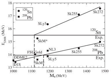
Figure 1: Centroid of the ISGMR in ²⁰⁸Pb and ¹²⁰Sn calculated with the constrained Hartree-Fock method versus the value of $M_{c}$ for various functionals. The experimental values for ²⁰⁸Pb and ¹²⁰Sn are taken from Refs.Lui2004 ; Li2007 ; Youngblood2004 , respectively, with respective error bars of $\pm 200$ and $\pm 100$ keV. This figure is taken from Ref.Khan2012 .

Rigorous analysis questioned the validity of the assumption of a strong correlation between $K_{0}$ and $E_{\scriptsize{GMR}}$ Colo2004 ; Khan2013 calculated from different forces, arguments were placed in favour of the fact that the ISGMR centroid $E_{\scriptsize{GMR}}$ maps the integral of the incompressibility $\int K(\rho)d\rho$ over the whole density rather than a single value at $\rho_{0}$. A larger value of $K(\rho_{0})$ for a given EDF can be compensated by a lower value of $K(\rho)$ at sub-saturation density so as to predict a similar value of ISGMR energy; as a result, $E_{\scriptsize{GMR}}$ might be a reflection of nuclear matter incompressibility at an effective density lower than $\rho_{0}$. Indeed, it is seen that $K(\rho)$ calculated with a multitude of EDFs when plotted against density cross each other at a density $\rho_{c}$ $[=(0.710\pm 0.005)\rho_{0}]$ Khan2012 . This universality possibly arises from the constraints encoded in the EDF from empirical nuclear observables. This crossing density $\rho_{c}$ looks more relevant as an indicator for the ISGMR centroid, with $K_{c}(\equiv K(\rho_{c}))$ found to be around $35\pm 4$ MeV Khan2013 . As the centroid energy $E_{\scriptsize{GMR}}$ maps the incompressibility integral, it seems, $E_{\scriptsize{GMR}}$ is more intimately correlated with $M(\rho_{c})$, the density derivative of $K(\rho)$ at the crossing density. The calculated values of $M(\rho_{c})$ from various EDFs are found to be linearly correlated with the corresponding $E_{\scriptsize{GMR}}$’s for both ²⁰⁸Pb and ¹²⁰Sn (see Fig. 1). From known experimental ISGMR data for the nuclei, a value of $M_{c}(\equiv M(\rho_{c}))\approx 1050\pm 100$ MeV Khan2013 is then obtained. Coming back to Eq. (13), with known values of $\rho_{c}$, $K_{c}$ and $M_{c}$ in conjunction with Eq. (15), the value of $a$ and $\tilde{\alpha}$ are calculated (we already assumed $e_{0}$, $\rho_{0}$ and $k_{+}$ to be known). The value of $K_{0}$ can now be related as

$$K\left(\rho_{0}\right)=K\left(\rho_{c}\right)+ \left(\rho-\rho_{c}\right)K^{\prime}\left(\rho_{c}\right)+\frac{\left(\rho-\rho_{c}\right)^{2}}{2}K^{\prime\prime}\left(\rho_{c}\right)+$$ (18)

$$+\left(\frac{\rho-\rho_{c}}{6}\right)^{3}K^{\prime\prime\prime}\left(\rho_{c}\right)+\cdots$$

The higher derivatives of $K(\rho)$ can be calculated recursively from Eq. (13). With chosen values of $e_{0}\sim-16.0$ MeV, $\rho_{0}\sim 0.155$ fm^-3 and $m^{\star}/m\sim 0.7$, $K_{0}$ comes out to be $\sim 212$ MeV De2015 . The first term in Eq. (18) is 35 MeV, the second term turns out to be 143.3 MeV, the third term is $35.9$ MeV, the fourth term is $-3.2$MeV and so on which adds up to $\sim 212$ MeV. Since ‘$a$’ and $\tilde{\alpha}$ are known, $Q_{0}$ and the other higher derivatives entering in Eq. (2) can be calculated thus defining the nuclear matter EoS, the first few terms giving a nearly precise description of the EoS around the saturation density. The value of $Q_{0}$ turns out to be $\sim-378$ MeV.

4 Asymmetric nuclear matter

We now consider asymmetric nuclear matter (ANM), a two component system consisting of neutrons and protons. To lowest order in the asymmetry parameter $\delta$, the energy of ANM contains, in addition to the SNM term (see Eq. (1)) a contribution $C_{2}(\rho)\delta^{2}$. The knowledge of $C_{2}(\rho)$ Eq. (3) involves understanding of its higher order density derivatives like $L_{0}$, $K_{\rm sym}^{0}$, etc. around $\rho_{0}$, in addition to $C_{2}^{0}$, the symmetry energy coefficient of ANM at $\rho_{0}$. In the following, we discuss on constraining the values of the symmetry elements through their correlations with various observables pertaining to finite nuclei and neutron stars. We further explore the possibility of plausible correlations among the symmetry elements themselves to see how the knowledge of known lower order symmetry elements can throw light on the values of the unknown higher order symmetry elements.

4.1 The symmetry energy coefficient

The value of $C_{2}^{0}$ is now known in very tight bounds Jiang2012 . The higher order density derivatives are, however, not very precisely known. The microscopic-macroscopic mass formula improved with the consideration of mirror nuclei constraint Wang2010 describes the binding energies in the entire nuclear mass table extremely well; removing the contributions of volume, surface, Coulomb, pairing and Wigner terms of this mass formula from the experimental binding energies, one is left with the symmetry energy that is called the ‘experimental symmetry energy’ $S(Z,A)$ for a nucleus with charge $Z$ and mass $A$. It may be a little approximate representation of the symmetry energy because of remnants of the effects due to shell structure, but the double differences of these experimental symmetry energies of neighboring nuclei (denoted by $\mathcal{R}_{ip-jn}(Z,A)$) effectively cancel the shell effects and then the double difference becomes a powerful tool for extracting the symmetry energy elements from the observed compact correlation of $\mathcal{R}_{ip-jn}(Z,A)[\mathcal{R}_{ip-jn}]$ with mass number $A$. The double difference is defined as

$$\mathcal{R}_{ip-jn}(Z,A)= S(Z,A)+S(Z-i,A-i-j)$$ (19)

$$-S(Z,A-j)-S(Z-i,A-i).$$

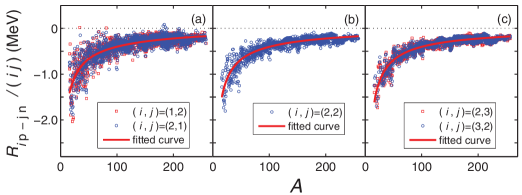
Figure 2: $R_{{ip-jn}}/(ij)$ (MeV) versus mass number $A$ . $R_{{ip}-{jn}}$ is given by double difference of experimental symmetry energies of four neighboring nuclei. Refer to the text for details. Panel (a): $(i,j)=(1,2)$ and (2,1), (b)$(i,j)$ =(2,2) and (c)$(i,j)=(2,3)$ and $(3,2)$ The solid red lines are used to guide the eyes. The figure is taken from Ref. Jiang2012 .

The values of $\mathcal{R}_{ip-jn}(Z,A)/(ij)$ are displayed in Fig. 2 for $(i,j)=(1,2),(2,1),(2,2)$ and $(3,2)$. No noticeable difference is seen between even-odd and odd-even nuclei, or between even-even and odd-odd nuclei for $\mathcal{R}_{ip-jn}$. Assuming

$$S(Z,A)=a_{\rm sym}(A)I^{2}A=(C_{\rm sym}^{v}-C_{\rm sym}^{s}A^{-1/3})I^{2}A,$$ (20)

an expression for $\mathcal{R}_{ip-jn}$ can be obtained in $C_{\rm sym}^{v}$ and $C_{\rm sym}^{s}$, which when fitted across the mass spectrum yields value for $C_{\rm sym}^{v}=32.10\pm 0.31$ MeV and for $C_{\rm sym}^{s}=58.91\pm 1.08$ MeV. In Eq. (20), $a_{\rm sym}(A)$ is the symmetry energy coefficient of a finite nucleus, the volume symmetry energy $C_{\rm sym}^{v}$ is identified with $C_{2}(\rho_{0})$ ($\equiv C_{2}^{0}$), $C_{\rm sym}^{s}$ is the surface symmetry energy coefficient and $I=(N-Z)/A$, the equivalent to the asymmetry parameter $\delta$ of ANM. The volume symmetry energy, so obtained does not differ significantly from that ($C_{2}(\rho_{0})=31.95\pm 1.75$MeV) obtained from analysis of excitation to isobaric analog states Danielewicz2014 augmented with empirical values of neutron skins determined using hadronic probes.

4.2 The density derivatives of symmetry energy

The density derivatives of the symmetry energy coefficients ($L_{0},K_{\rm sym}^{0}$ etc) are not yet known with desirable certainty. Calculations with selective Skyrme and relativistic EDFs show a nearly linear correlation of $C_{2}^{0}$ with $L_{0}$ Carbone2010 ; Tsang2012 ; Danielewicz2014 ; Lattimer2016 pointing to a value of the symmetry derivative $L_{0}$. In a considerable density range around $\rho_{0}$, it has been found that the ansatz

$$C_{2}(\rho)=C_{2}(\rho_{0})(\frac{\rho}{\rho_{0}})^{\beta},$$ (21)

works well Chen2005 ; Li2008 , where $\beta$ is a constant $\sim 0.69$. Then $L_{0}=\left.3\rho_{0}\frac{\partial C_{2}}{\partial\rho}\right|_{\rho_{0}}=3\beta C_{2}^{0}.$ In Ref. Carbone2010 , with a few Skyrme interactions. a nearly linear correlation of $L_{0}$ with $C_{2}^{0}$ has been reported. This is, however, approximate. The tendency of a larger $L_{0}$ with larger $C_{2}^{0}$ can not be overlooked though. Different nuclear physics observables like isospin diffusion, nuclear emission ratio, isoscaling, giant dipole resonances, pygmy dipole resonance etc Li2008 ; Famiano2006 ; Shetty2007 ; Trippa2008 ; Carbone2010 hint at a central value of $L_{0}$, all differing from each other, astronomical data on neutron star masses and radii providing a further different value Steiner2012 . In a novel exercise involving the nuclear Droplet Model (DM), Centelles et al Centelles2009 ; Warda2009 showed that the neutron-skin $\Delta r_{np}$ of a nucleus can be recast to leading order in $L_{0}$ lending a good linear fit of $\Delta r_{np}$ with $L_{0}$ (see Fig. 3). With $\Delta r_{np}$ known from hadronic probes, a value of $L_{0}=75\pm 25$ MeV was arrived at. In the ambit of microscopic calculations with different EDFs, this idea was advanced further, the correlation of the neutron-skin thickness with $L_{0}$ helped to find $L_{0}$ in narrower limits Agrawal2012 ; Agrawal2013 . However the estimates on neutron skin thickness based on the hadronic probes are model dependent. The ²⁰⁸Pb Radius EXperiment (PREX) and ⁴⁸Ca Radius EXperiment CREX experiments based on the electroweak probe would allow the model independent determination of the neutron skin thickness in ²⁰⁸Pb and ⁴⁸Ca nuclei. These experiments are designed to extract the neutron skin thickness from parity violating electron scattering. The extracted ²⁰⁸Pb skin thickness $\Delta r_{np}=0.33^{+0.16}_{-0.18}$ fm Abrahamyan2012 has very large statistical uncertainty. The future experiment PREX-II is designed to achieve the originally proposed experimental precision in $\Delta r_{np}$ to $1$ % PREX-II . The CREX is expected to provide precision in $\Delta r_{np}$ of ⁴⁸Ca to $0.6$% CREX . The ⁴⁸Ca being a light nucleus may provide the key information for bridging ab initio calculations and those based on the density functional theories.

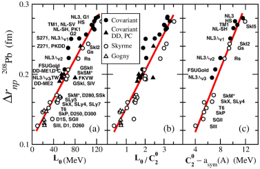
Figure 3: Correlation of the neutron-skin thickness $\Delta r_{np}$ for ²⁰⁸Pb with the slope of the symmetry energy $L_{0}$ (a), the ratio $L_{0}/C_{2}^{0}$ (b), and with $C_{2}^{0}-a_{\rm sym}(A)$ (c), for various nuclear models ( DD and PC stand for density dependent and point coupling models). From left to right, the correlation factors are $r=0.961,0.945,$ and $0.970$. The figure is taken from Ref.Centelles2009 .

The shroud of uncertainty looms larger on the higher symmetry derivatives $K_{\rm sym}^{0}(=K_{\rm sym}(\rho_{0})=9\rho_{0}^{2}\frac{\partial^{2}C_{2}}{\partial\rho^{2}}|_{\rho_{0}}$) and $Q_{\rm sym}^{0}(=Q_{\rm sym}(\rho_{0})=27\rho_{0}^{3}\frac{\partial^{3}C_{2}}{\partial\rho^{3}}|_{\rho_{0}})$. The values of $K_{\rm sym}^{0}$ and $Q_{\rm sym}^{0}$, in different parameterizations of the Skyrme EDFs lie in very wide ranges [-700 MeV $<K_{\rm sym}^{0}<+400$MeV, -800 MeV $<Q_{\rm sym}^{0}<1500$ MeV] Dutra2012 ; Dutra2014 . From the ansatz in Eq. (21), it is seen that $K_{\rm sym}^{0}=3(\beta-1)L_{0}$ and so should have a perfect linear correlation with $L_{0}$ when $\beta$ is a constant. Danielewicz and Lee Danielewicz2009 have shown a linear relationship between $K_{\rm sym}^{0}$ and $L_{0}$, studied with 118 Skyrme EDFs,. Tews et al Tews2017 propose a relation of the form:

$$K_{\rm sym}^{0}\approx 3.41L_{0}-306\pm 40~{}{\rm MeV}.$$ (22)

Mondal et al Mondal2018 , with a total of 237 Skyrme EDFs also find a correlation between them, but the correlation is not very strong (correlation coefficient $r\sim 0.8$); the correlation becomes more robust only when a selected subset of 162 EDFs are chosen ($r\sim 0.91$). These 162 Skyrme EDFs are selected by constraining the iso-scalar nucleon effective mass $\frac{m_{0}^{*}}{m}$ to $0.85\pm 0.15$ and the isovector splitting of effective mass $\mid{\frac{m_{n}^{\star}-m_{p}^{\star}}{m}}\mid$ to less than unity, which more than covers the values from the limited experimental data Zhang2016 ; Coupland2016 ; Kong2017 and recent theoretical values on it.

4.3 Interrelating symmetry elements

Starting from a plausible set of approximations on the nucleonic interaction (density dependent, quadratically dependent on momentum) as stated in the beginning of Sec.3, for asymmetric nuclear matter, the equation for the energy per nucleon can be generalized from Eq. (10) to

$$e(\rho,\delta)=\frac{1}{\rho}\left[\sum_{\tau}\frac{P_{F,\tau}^{2}}{10m}\rho_{\tau}\left(3-2\frac{m}{m_{\tau}^{\star}(\rho)}\right)\right]-V_{2}(\rho,\delta)+\frac{P(\rho,\delta)}{\rho}.$$ (23)

Here $\tau$ is the isospin index, $\rho_{\tau}=(1+\tau\delta)\frac{\rho}{2};\tau=1$ for neutrons and -1 for protons. The Fermi momentum of the component nucleonic matter can be written as $P_{F,\tau}=g_{2}\rho_{\tau}^{1/3}$ with $g_{2}=(3\pi^{2})^{1/3}\hbar$. The effective mass for the two component nuclear matter, to lowest order in $\rho$ is written as

$$\frac{m}{m_{\tau}^{\star}(\rho)}=1+\frac{k_{+}}{2}\rho+\frac{k_{-}}{2}\rho\tau\delta,$$ (24)

and the rearrangement potential generalized for ANM

$$V_{2}(\rho,\delta)=\left(a+b~{}\delta^{2}\right)\rho^{\tilde{\alpha}}.$$ (25)

The new constant $b$ is a measure of the asymmetry dependence of the rearrangement potential. Since, $P=\rho^{2}\frac{\partial e}{\partial\rho}$, Eq. (23) can be integrated Malik2018a

$$e(\rho,\delta)= \frac{3}{10}\gamma\left[\sum_{\tau}\left(1+\tau~{}\delta\right)^{5/3}\left\{\rho^{2/3}+\frac{1}{2}\rho^{5/3}\left(k_{+}+k_{-}\tau~{}\delta\right)\right\}\right]$$ (26)

$$+\left(a+b~{}\delta^{2}\right)\frac{\rho^{\tilde{\alpha}}}{(\tilde{\alpha}-1)}+K(\delta)\rho,$$

where, $\gamma=g_{2}^{2}/(2^{5/3}m)$ and $K(\delta)=(K_{1}+K_{2}\delta^{2}+K_{4}\delta^{4}+...)$ is a constant of integration. The symmetry coefficient $C_{2}(\rho)(=\frac{1}{2}\frac{\partial^{2}e}{\partial\delta^{2}}|_{\delta=0})$ is then derived as

$$C_{2}(\rho)=\frac{b\rho^{\tilde{\alpha}}}{(\tilde{\alpha}-1)}+\frac{\gamma}{3}\rho^{2/3}\left[1+\frac{1}{2}\left(k_{+}+3k_{-}\right)\rho\right]+K_{2}\rho,$$ (27)

so also $L(\rho)$ and $K_{\rm sym}(\rho)$,

$$L(\rho)=\frac{3\tilde{\alpha}}{(\tilde{\alpha}-1)}b\rho^{\tilde{\alpha}}+\frac{2}{3}\gamma\rho^{2/3}+\frac{5}{6}\gamma\rho^{5/3}\left(k_{+}+3k_{-}\right)+3K_{2}\rho,$$ (28)

$$K_{\rm sym}(\rho)=9\tilde{\alpha}b{\rho^{\tilde{\alpha}}}-\frac{2}{3}\gamma\rho^{2/3}+\frac{5}{3}\gamma\rho^{5/3}\left(k_{+}+3k_{-}\right).$$ (29)

A little algebra then leads to an equation interrelating $C_{2}^{0},L_{0}$ and $K_{\rm sym}^{0}$

$$K_{\rm sym}^{0}=-5\left[3C_{2}^{0}-L_{0}\right]+3b\rho_{0}^{\tilde{\alpha}}(3\tilde{\alpha}-5)+E_{F}^{0}.$$ (30)

We note at this point that the r.h.s of Eq. (23) can be expanded in powers of $\delta$ using expressions for $P$ and $V_{2}(\rho,\delta)$. Comparing with Eq. (1) and equating coefficients of the same order in $\delta$ one gets an expression for $C_{2}(\rho)$ (it looks somewhat different Mondal2017 from that given in Eq. (27) though they are equivalent)

$$C_{2}(\rho)=-b\rho^{\tilde{\alpha}}+\rho\frac{\partial C_{2}}{\partial\rho}+\frac{\gamma}{9}\rho^{2/3}\left[1-\left(k_{+}+3k_{-}\right)\rho\right].$$ (31)

This leads to expressions for $K_{\rm sym}^{0}$ and $Q_{\rm sym}^{0}$ as,

$$K_{\rm sym}^{0}=-3\tilde{\alpha}\left[3C_{2}^{0}-L_{0}\right]+E_{F}^{0}\left[(3\tilde{\alpha}-4)+\left(\frac{2}{3}\frac{m}{m_{0}^{\star}}+k_{-}~{}\rho_{0}\right)(5-3\tilde{\alpha})\right],$$ (32)

and

$$Q_{\rm sym}^{0}=15\tilde{\alpha}\left[3C_{2}^{0}-L_{0}\right]+K_{\rm sym}^{0}(3\tilde{\alpha}-1)+E_{F}^{0}(2-3\tilde{\alpha}).$$ (33)

Eqs. (32) and (33) show that there is an interrelationship between $K_{\rm sym}^{0}$ and $Q_{\rm sym}^{0}$. Making use of Eq. (30), one gets :

$$K_{\rm sym}^{0}+Q_{\rm sym}^{0}=9b\rho_{0}^{\tilde{\alpha}}\tilde{\alpha}(3\tilde{\alpha}-5)+E_{F}^{0}.$$ (34)

Eq. (30) looks very similar to that obtained for the correlations among $C_{2}^{0}$, $L_{0}$ and $K_{\rm sym}^{0}$ in Skyrme models Mondal2018 . This is not coincidental. There is an exact equivalence of the Skyrme functional with the EDF given by Eq. (26) provided the term $K(\delta)$ is truncated at $\delta^{2}$. The parameters $\tilde{\alpha},K_{1},K_{2}$ etc. can then be correlated to the standard Skyrme parameters Malik2018a

$$\tilde{\alpha}=\alpha+1$$

$$K_{1}=\frac{3}{8}t_{0}$$

$$K_{2}=-\frac{1}{4}t_{0}\left(x_{0}+\frac{1}{2}\right)$$

$$a=\frac{1}{16}t_{3}\alpha$$

$$b=-\frac{1}{24}t_{3}\left(x_{3}+\frac{1}{2}\right)\alpha$$

$$k_{+}=\frac{m}{\hbar^{2}}\left[\frac{3}{4}t_{1}+\frac{5}{4}t_{2}+t_{2}x_{2}\right]$$

$$k_{-}=\frac{m}{2\hbar^{2}}\left[t_{2}\left(x_{2}+\frac{1}{2}\right)-t_{1}\left(x_{1}+\frac{1}{2}\right)\right].$$ (35)

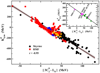
Figure 4: The correlation between $K_{\mathrm{\rm sym}}^{0}$ and $\left[3C_{2}^{0}-L_{0}\right]$ as obtained from 500 EDFs Dutra2012 ; Dutra2014 . The black circles correspond to the Skyrme-inspired EDFs, and the red squares refer to those obtained from RMF models. The models consistent with all the constraints demanded by Dutra et al.Dutra2012 are highlighted by orange circles for Skyrme EDFs Dutra2012 and blue squares for RMF EDFs Dutra2014 . The inner (outer) colored regions around the best-fit straight line through these points depict the loci of $95\%$ confidence (prediction) bands of the regression analysis. The inset shows the correlation line obtained from the Skyrme-RMF models, and the magenta triangles are the results obtained from EDFs with realistic interactions, $\mathrm{MDI}(0),\mathrm{MDI}(1),\mathrm{MDI}(-1)$Chen2009 APR Akmal1998 , BHF Taranto2013 , BCPM Baldo2013 , and $\mathrm{SBM}$Agrawal2017 , respectively. The green diamonds represent results from a few Gogny interactions Sellahewa2014 . The figure is taken from Mondal2017 .

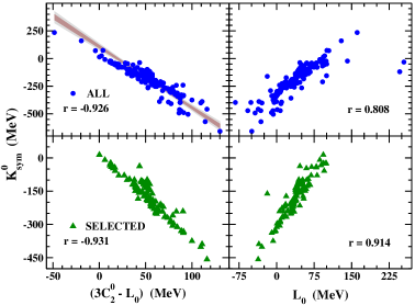
Figure 5: The correlation of $K_{\rm sym}^{0}$ with $L_{0}$ and with $\left[3C_{2}^{0}-L_{0}\right]$ are depicted in the right and left panels respectively. Results for 237 Skyrme EDFs (’ALL’) are displayed in the upper panels, the lower panels contain the results for a selected subset of 162 models (’SELECTED’) (see text for details). The inner(outer) colored regions around the best-fit straight line in upper left panel depict the loci of $95\%$ confidence (prediction) bands of the regression analysis. The figure is taken from Ref. Mondal2018 .

The structure of Eq. (30) and Eq. (32) shows that there is a strong likelihood of a linear correlation between $(3C_{2}^{0}-L_{0})$ and $K_{\rm sym}^{0}$. Realizing that the EDF was obtained from general thermodynamical considerations and some very plausible assumptions on the nature of the nuclear force, one may expect this correlation to be universal; this is vindicated from the correlated structure of $K_{\rm sym}^{0}$ with $(3C_{2}^{0}-L_{0})$ as displayed in Fig. 4 for 500 EDFs Dutra2012 ; Dutra2014 that have been in use to explain nuclear properties. The correlation is seen to be very robust, the correlation coefficient $r=-0.95$ . In the inset of the figure, results corresponding to EDFs obtained from several realistic interactions (magenta triangles) and a few Gogny interactions (green diamonds) are also displayed. They lie nearly on the correlation line highlighting further the universality in the correlation. Imposing a general constraint that the neutron energy per particle should be zero at zero density of neutron matter, a plausible explanation of such a correlation was given recently Margueron2018 . The linear regression analysis yields

$$K_{\rm sym}^{0}=d_{1}\left(3C_{2}-L_{0}\right)+d_{2},$$ (36)

with $d_{1}=-4.97\pm 0.07$ and $d_{2}=66.80\pm 2.14$ MeV. One sees that $d_{1}$ is very close to $-5$ as expected form Eq. (30). In a recently developed density dependent Van der Waals model for nuclear matter, with some constraints on $K_{0}$, exactly such a relation was found Dutra2020 where $d_{1}=-6.3$ and $d_{2}=51.5$ MeV. As mentioned earlier, from Eq. (22) one also expects a correlation between $K_{\rm sym}^{0}$ and $L_{0}$, but it is comparably weaker (see Fig. 5). With a total of 237 Skyrme EDFs Mondal et al Mondal2018 looked for correlation between $Q_{\rm sym}^{0}$ and $(3C_{2}^{0}-L_{0})$ and also with $L_{0}$. The correlation found was poor, only with a selected subset of Skyrme models as discussed earlier, an improved correlation was found (see Fig. 6 ).

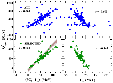
Figure 6: Same as Fig.5, but for $Q_{\rm sym}^{0}$. The confidence bands of regression analysis are given only for the subset of models (’SELECTED’) in the lower left panel. The figure is taken from Ref.Mondal2018 .

Estimates of the symmetry elements $L_{0},K_{\rm sym}^{0}$ etc., were made by Centelles et al Centelles2009 from the correlation systematics of $L_{0}$ with the neutron-skin of nuclei obtained from hadronic probes. The neutron skins have large uncertainties, so do $L_{0}$. From equations we have set up, we show that knowledge of the symmetry energy at another density (but for $\rho_{0}$), say a sub-saturation density $\rho_{1}$, helps to find a more controlled value of $L_{0}$. We choose the value of $C_{2}(\rho_{1})(=24.1\pm 0.8$ MeV) at $\rho_{1}=0.1$ fm^-3 found from its strong correlation with the centroid of the GDR resonance energy in spherical nuclei in Skyrme EDFs Trippa2008 . An initial estimate of $L_{0}$ can be done from Eqs. (3) and (36). Leaving out terms beyond $\epsilon^{2}$ in Eq. (3) (which may not be a very bad approximation), with $C_{2}^{0}=32.1\pm 0.3$ MeV, $\rho_{0}=0.155\pm 0.008$ fm^-3, $C_{2}(\rho_{1})$ and $\rho_{1}$ being just mentioned, one gets $L_{0}\sim 61.3$ MeV. A more dependable value is, however, obtained from an input value of the effective mass $m_{0}^{*}$.

Then, keeping terms upto $Q_{\rm sym}^{0}$ in Eq. (3), from Eqs. (33) and (36), $L_{0}$, $K_{\rm sym}^{0}$, $Q_{\rm sym}^{0}$ can be calculated. For the effective mass, a value of $m_{0}^{*}/m=0.70\pm 0.05$ is taken that is consistent with many analyses Jaminon1989 ; Li2015 . The value of the symmetry elements then turn out to be $L_{0}=60.3\pm 14.5$ MeV, $K_{\rm sym}^{0}=-111.8\pm 71.3$ MeV, and $Q_{\rm sym}^{0}=296.8\pm 73.6$ MeV. The value of $k_{-}$ can be calculated from Eq.(32). It is a measure of the isovector effective mass splitting $\Delta m_{0}^{*}$ at asymmetry $\delta$,

$$\Delta m_{0}^{\star}=\left(\frac{m_{n}^{\star}-m_{p}^{\star}}{m}\right)_{\rho_{0}}\cong-k_{-}\rho_{0}\left(\frac{m_{0}^{\star}}{m}\right)^{2}\delta.$$ (37)

Its value turns out to be $\Delta m_{0}^{*}=(0.17\pm 0.24)\delta$.

4.4 Electric dipole polarizability: relations to symmetry elements

Under the action of an isovector probe, semi-classically speaking, the centers of the neutron and the proton fluids separate leading to an electric dipole polarization in the nucleus. The dipole polarizability $\alpha_{D}$ is defined as,

$$\alpha_{D}=\frac{8\pi e^{2}}{9}\int_{0}^{\infty}\omega^{-1}\mathcal{R}\left(\omega,E_{1}\right)d\omega=\frac{8\pi e^{2}}{9}m_{-1}(E_{1}).$$ (38)

Here $R(\omega,E1)$ is the electric dipole strength as a function of the excitation energy $\omega$ and $m_{-1}(E1)$ is called the inverse energy weighted sum rule for the electric dipole $(E1)$ excitations. The dipole polarizability is an experimentally measurable quantity and thus becomes an effective indicator of the symmetry elements related to asymmetric nuclear matter. The $m_{-1}$ moment may be obtained with the random-phase-approximation ( RPA) methodology, the so-called dielectric theorem Bohigas1979 ; Hinohara2015 also allows to extract it from a constrained ground state calculation. It is related to the constrained energy $E_{x}$ Bohigas1979 as

$$\left(\frac{m_{-1}}{m_{1}}\right)^{1/2}=1/E_{x},$$ (39)

where $m_{k}$ is the $kth$ moment of the energy weighted sum rule (EWSR)

$$m_{k}=\int d\omega\quad\omega^{k}\quad\mathcal{R}\left(\omega,E_{1}\right).$$ (40)

Solving the constrained problem classically in the ambit of the Droplet Model (DM) Myers1974 , it was shown Meyer1982 that for a nucleus of mass $A$ , the dipole polarizability can be written in terms of the symmetry energy constant $C_{2}^{0}$ as

$$\alpha_{D}^{\rm DM}=\frac{\pi e^{2}}{54}\frac{A\left\langle r^{2}\right\rangle}{C_{2}^{0}}\left(1+\frac{5}{3}\times\frac{9}{4}\frac{C_{2}^{0}}{Q}{A}^{-1/3}\right).$$ (41)

In Eq.(41), $<r^{2}>$ is the mean-square radius of the nucleus and $Q$ the surface stiffness constant, a measure of the resistance of the motion of neutrons against protons. Eq. (41) has a few consequences. The ratio $C_{2}^{0}/Q$ and the density slope parameter $L_{0}$ are known to show a strong linear correlation Warda2009 ; Centelles2009 for a large set of EDFs, the electric dipole polarizability is therefore expected to be very closely tied to the symmetry properties of asymmetric nuclear matter. The DM relates the symmetry energy coefficient $a_{\rm sym}(A)$ of a finite nucleus with $C_{2}^{0}/Q$ as

$$a_{\rm sym}(A)=\frac{C_{2}^{0}}{1+\frac{9}{4}\frac{C_{2}^{0}}{Q}A^{-1/3}}.$$ (42)

Expanding Eq. (42) to first order in the small parameter $\frac{C_{2}^{0}}{Q}A^{-1/3}$, Eq. (41) may be written as

$$\alpha_{D}^{DM}\approx\frac{\pi e^{2}}{54}\times\frac{A<r^{2}>}{C_{2}^{0}}\quad\left(1+\frac{5}{3}\frac{C_{2}^{0}-a_{\rm sym}(A)}{C_{2}^{0}}\right).$$ (43)

Since $C_{2}^{0}-a_{\rm sym}(A)=a_{\rm sym}^{s}A^{-1/3}$, where $a_{\rm sym}^{s}$ is the surface symmetry term, it is evident that $\alpha_{D}^{DM}$ is sensitive to the ratio of the surface and bulk symmetry energies. Since,

$$a_{\rm sym}(A)\approx C_{2}\left(\rho_{A}\right),$$ (44)

where $\rho_{A}$ is close to the average density of a nucleus (which is necessarily lower than $\rho_{0}$), Eq. (43) shows that the symmetry energy at the sub-saturation density $\rho_{A}$ can be gauzed RocaMaza2013 if the dipole polarizability is known. In Ref. Centelles2009 , $\rho_{A}$ for ²⁰⁸Pb is taken as $\sim 0.1$ fm^-3. In Ref. Agrawal2012 , it is shown how to evaluate it in a local density approximation. From Eq. (3), to lowest orders, $C_{2}(\rho_{A})$ can be written as $C_{2}(\rho_{A})=C_{2}^{0}+L_{0}\epsilon_{A}$, using this in Eq. (41) results in

$$\alpha_{D}^{\rm DM}\approx\frac{\pi e^{2}}{54}\frac{A<r^{2}>}{C_{2}^{0}}\left[1-\frac{5}{3}\frac{L_{0}}{C_{2}^{0}}\epsilon_{A}\right],$$ (45)

where $\epsilon_{A}=(\rho_{A}-\rho_{0})/3\rho_{0}$. This formula is suggestive of a close relationship between $\alpha_{D}$ and the symmetry elements $L_{0}$ and $C_{2}^{0}$. Indeed, it has been seen with Skyrme and six different families of systematically varied EDFs that $\alpha_{D}C_{2}^{0}$ has a nearly linear relationship with $L_{0}$ RocaMaza2013 as seen in Fig. 7. Specifically with an adopted value of $C_{2}^{0}=(31\pm 2_{\rm est})$ MeV, it is found that

$$L_{0}=43\pm 6_{exp}\pm 8_{theo}\pm 12_{est}~{}{\rm MeV},$$ (46)

where ’est’ refers to the uncertainties derived from different estimates on $C_{2}^{0}$.

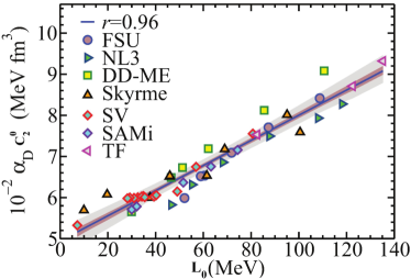
Figure 7: Dipole polarizability in ²⁰⁸ Pb times the symmetry energy at saturation as a function of the slope parameter $L_{0}$ calculated with some modern EDFs (see Ref.RocaMaza2013a for further details). The linear fit gives $10^{-2}\alpha_{D}C_{2}^{0}=(4.80\pm 0.04)+(0.033\pm 0.001)L_{0}$ with a correlation coefficient $r=0.96,$ and the two shaded regions represent the $99.9\%$ and $70\%$ confidence bands. This figure is taken from Ref.RocaMaza2013a

.

The simplicity of the DM allows one to extract a relationship between $\alpha_{D}$ and the neutron-skin thickness $\Delta r_{np}$. In terms of the bulk nuclear matter properties, the neutron skin in DM can be written as Centelles2009 ,

$$\Delta r_{np}=\sqrt{\frac{3}{5}}\left[\frac{3r_{0}}{2}\frac{\frac{C_{2}^{0}}{Q}(I-I_{\scriptsize{C}})}{1+\frac{9}{4}\frac{C_{2}^{0}}{Q}A^{-1/3}}\right]+\Delta r_{np}^{coul}+\Delta r_{np}^{surf},$$ (47)

where $I=(N-Z)/A$ is the relative neutron excess in the nucleus, $I_{\scriptsize{C}}=e^{2}Z/(20C_{2}^{0}R),R=r_{0}A^{1/3},r_{0}=(\frac{3}{4\pi\rho_{0}})^{1/3},\Delta r_{np}^{coul}=-\sqrt{3/5}(e^{2}Z)/(70C_{2}^{0})$ is the correction caused by electrostatic repulsion and $\Delta r_{np}^{surf}=\sqrt{3/5}[5(b_{n}^{2}-b_{p}^{2})/2R]$, a correction coming from the difference in surface widths of the neutron and proton density profiles Myers1980 . Expanding Eq. (47)to first order in $\frac{C_{2}^{0}}{Q}A^{-1/3}$, a little algebra RocaMaza2013 gives the following relation,

$$\alpha_{D}^{DM}\approx\frac{\pi e^{2}}{54}\frac{A<r^{2}>}{C_{2}^{0}}[1+\frac{5}{2}\frac{\Delta r_{np}^{DM}-\Delta r_{np}^{coul}-\Delta r_{np}^{surf}}{<r^{2}>^{1/2}(I-I_{\scriptsize{C}})}].$$ (48)

With an adopted value of $C_{2}^{0}=31\pm 2$ MeV, one finds for ²⁰⁸Pb that $I_{\scriptsize{C}}\approx 0.028\pm 0.002,\Delta r_{np}^{coul}\approx-0.042\pm 0.003$ fm. It was further shown for ²⁰⁸Pb from a large number of EDFs that $\Delta r_{np}^{\rm surf}\approx 0.09\pm 0.01$ fmCentelles2010 . Consequently, the small variations in $\Delta r_{np}^{\rm coul},\Delta r_{np}^{\rm surf}$ and $I_{\scriptsize{C}}$ can reasonably be ignored, resulting in, to a good approximation,

$$\alpha_{D}^{DM}\approx\frac{\pi e^{2}}{54}\frac{A<r^{2}>}{C_{2}^{0}}[1+\frac{5}{2}\frac{\Delta r_{np}^{DM}}{I<r^{2}>^{1/2}}].$$ (49)

Eq. (49) suggests a strong correlation between $\alpha_{D}C_{2}^{0}$ with the neutron skin. This tight correlation (see Fig. 8) was validated RocaMaza2013a in a self-consistent mean-field plus RPA calculation for both neutron-skin thickness and electric dipole polarizability using a large set of representative non-relativistic and relativistic models. If the symmetry energy coefficient $C_{2}^{0}$ and $\alpha_{D}$ are known in good precision, a consequence of this correlation is a pointer to the value of the neutron-skin thickness. Combining the measured value of $\alpha_{D}$ Tamii2011 for ²⁰⁸Pb with the adopted value of $C_{2}^{0}$ as mentioned, the neutron skin thickness of ²⁰⁸Pb is predicted to be,

$$\Delta r_{np}=0.165\pm(0.009)_{exp}\pm(0.013)_{theo}\pm(0.021)_{est}{\rm fm}.$$ (50)

It is to be noted that in the DM model $\alpha_{D}C_{2}^{0}$ is better correlated to $\Delta r_{np}$ rather than $\alpha_{D}$ alone to $\Delta r_{np}$RocaMaza2013a ; this is in contravariance to that obtained in Refs. Tamii2011 ; Reinhard2010 .

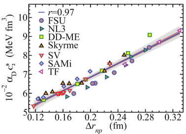
Figure 8: Dipole polarizability times the symmetry energy at saturation of each model against the neutron skin thickness in ²⁰⁸Pb predicted by the EDFs of Fig. 7. The linear fit gives $10^{-2}\alpha_{D}C_{2}^{0}=(3.01\pm 0.32)+(19.22\pm 0.73)\Delta r_{\mathrm{np}}$ with a correlation coefficient $r=0.97,$ and the two shaded regions represent the $99.9\%$ and $70\%$ confidence bands. This figure is taken from Ref. RocaMaza2013a .

4.5 The isovector and isoscalar mass: nucleon isovector mass splitting

Experimental data on dipole polarizability Birkhan2017 ; Hashimoto2015 ; Tamii2011 ; Rossi2013 add new to the wealth of information on atomic nuclei and can be exploited to gain more confidence on the nuclear matter parameters entering the EoS. In the following, we show how it aids in guiding to the nuclear matter EoS, to finding the isovector nucleon mass , the isovector splitting of nucleon mass and then the other nuclear matter parameters Malik2018a . The isovector nucleon mass $m_{v,0}^{*}$ is the effective mass of a proton in pure neutron matter or vice versa, and is defined as

$$\frac{m}{m_{v,0}^{*}}=1+\frac{m}{2\hbar^{2}}\rho_{0}\Theta_{v},$$ (51)

where

$$\Theta_{v}=\frac{\hbar^{2}}{2m}(k_{+}-k_{-}).$$ (52)

We have already seen that $k_{+}$ gives the isoscalar nucleon mass and $k_{-}$ (from Eq. (37)) defines the isovector mass splitting. In Skyrme methodology, one can check from Eq. (4.3) that the isovector parameter $\Theta_{v}$ is,

$$\Theta_{v}=t_{1}(1+x_{1}/2)+t_{2}(1+x_{2}/2).$$ (53)

The energy weighted sum rule $m_{1}$ (see Eq. (40) for the isovector giant dipole resonance (IVGDR) of a nucleus can be written as Bohr1975 ,

$$m_{1}=\frac{9}{4\pi}\frac{\hbar^{2}}{2m}\frac{NZ}{A}(1+\kappa_{A}),$$ (54)

where $\kappa_{A}$ is the polarizability enhancement factor for the nucleus. It has a relation to $\Theta_{v}$ as Chabanat1997 ,

$$\kappa_{A}=\frac{2m}{\hbar^{2}}\frac{A}{4NZ}\Theta_{v}\times I_{A},$$ (55)

where the integral $I_{A}=\int\rho_{n}(r)\rho_{p}(r)d^{3}r$, $\rho_{n}(r)$ and $\rho_{p}(r)$ being the neutron and proton density distributions in the nucleus. In principle, $m_{1}$ can be determined from the experimental strength function $R(\omega)$, $\kappa_{A}$ is then determined. If $I_{A}$ is known from some other source, then $\Theta_{v}$, and hence the isovector mass can be calculated. If the isoscalar effective mass is further known, one gets $k_{-}$ and thence the isovector mass splitting $\Delta m_{0}^{*}$. Any knowledge of the dipole polarizability $\alpha_{D}$ is redundant in the extraction of $\Theta_{v}$, it appears.

The fact that the high energy component of the strength function is plagued with ’quasi-deuteron effect’ renders the determination of $m_{1}$ not very reliable; this forces us to look into dipole polarizability as an extra experimental input. From Eqs. (38) and (39), $m_{1}$ is written as,

$$m_{1}=\frac{9}{8\pi e^{2}}E_{x}^{2}\alpha_{D}.$$ (56)

To find the values of $\Theta_{v}$, values of $m_{1}$ are constructed from reasonable inputs on the constrained energy $E_{x}$ and the integrals $I_{A}$, which are found from correlation systematics.

We first find the isovector integrals $I_{A}$. From the neutron and proton densities $\rho_{n}(r)$ and $\rho_{p}(r)$ calculated in the Hartree-Fock (HF) approximation for the four nuclei, viz, ⁴⁸Ca, ⁶⁸Ni, ¹²⁰Sn and ²⁰⁸Pb (for which the data for $\alpha_{D}$ are available) with selected Skyrme EDFs (called ’best-fit’ Skyrme EDFs Brown2013 ), it is found that the integrals $I_{A}$ for a particular nucleus are nearly independent of EDFs Malik2018a . The values of $m_{1}$ calculated from the HF +RPA and hence $\kappa_{A}$ are different for different EDFs with differing values of $\Theta_{v}$, but there is an extremely strong correlation (with correlation coefficient $r$ practically unity) between $\Theta_{v}$ and $\kappa_{A}$ as displayed in Fig. 9. The slopes of the correlation lines are taken as measures for $I_{A}$ for each nuclei; they are shown in respective panels in the figure.

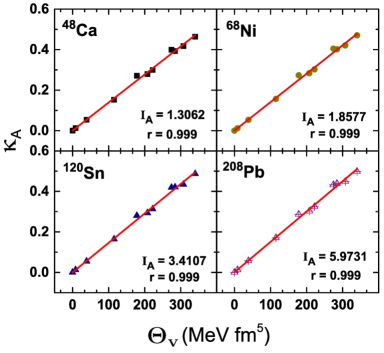
Figure 9: The correlation of the isovector parameter $\Theta_{v}$ obtained from the Skyrme EDFs Brown2013 with the calculated dipole enhancement factor $\kappa_{A}$ for the nuclei ${}^{48}\mathrm{Ca},^{68}\mathrm{Ni},^{120}\mathrm{Sn}$, and ${}^{208}\mathrm{Pb}$. The corresponding values of the integrals $I_{A}$ (in units of $\mathrm{fm}^{-3}$ ) and the correlation coefficients are shown in each panel. The figure is taken from Ref. Malik2018a .

As noted already, experimental values of $m_{1}$ are somewhat uncertain due to ’quasi-deuteron’ effect. With reasonable choice of the constraint energy $E_{x}$, we try to gauze $m_{1}$ in good bounds from existing data on $\alpha_{D}$ for the four nuclei as mentioned. Two choices of $E_{x}$ are made. For the lower values of $E_{x}$, the known peak energy $E_{p}$ of the experimental IVGDR strength function is chosen. For the higher value, $E_{x}=1.05E_{p}$ is taken. This choice is not arbitrary, in RPA calculations with the ’best-fit’ Skyrme EDFsBrown2013 , it has always been found that $E_{x}$ is higher than $E_{p}$ by $\sim(4-6)\%$ for the nuclei studied. These two choices of $E_{x}$ provide the lower and upper bounds of $m_{1}$.

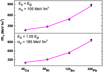
Figure 10: The calibrated values of EWSR $\left(m_{1}\right)$ displayed for the four nuclei (black squares). The upper panel shows the values with $E_{x}=E_{p},$ the lower panel displays the same with $E_{x}=1.05E_{p}$ (see text for details). The solid lines are drawn to show the fit with $\Theta_{v}=105~{}\mathrm{MeV}\mathrm{fm}^{5}$ and $185~{}\mathrm{MeV}\mathrm{fm}^{5},$ respectively. The figure is taken from Ref. Malik2018a .

The value of $\Theta_{v}$ is then obtained as follows: $E_{x}$ equated with $E_{p}$, $m_{1}$ calculated from Eq. (56) for the four nuclei with the experimental values of $\alpha_{D}$, $\kappa_{A}$ obtained from Eq. (54). With known values of $I_{A}$, the so-obtained $\kappa_{A}$ are then subjected to a $\chi^{2}$ minimization by varying $\Theta_{v}$ (Eq. (55)). The optimized value of $\Theta_{v}$ is found to be $\Theta_{v}=105.0$ MeV fm⁵. The calculation is repeated with $E_{x}=1.05E_{p}$. The optimized value of $\Theta_{v}$ is now 185.0 MeV fm⁵. The fitted two sets of results are shown in Fig. 10. The fits are seen to be very good in both cases. An average value of $\Theta_{v}\approx 145.0\pm 40.0$ MeV fm⁵ can be inferred from the calculation. Since, $\Theta_{v}$ is the difference between $k_{+}$ and $k_{-}$ and is a constant, if $k_{+}$ increases $k_{-}$ should also increase or vice versa. The dipole polarizability then helps to find the isovector parameter $\Theta_{v}$ or the isovector mass $m_{v,0}^{*}$, but does not give directions to separately find $k_{+}$ (the isoscalar mass $m_{0}^{*}$) or $k_{-}$ (the isovector mass splitting $\Delta m_{0}^{*}$).

Inference on the value of the effective isoscalar mass $m_{0}^{*}$ has been drawn from many corners; they seem to lie in a rather broad range. Skyrme EDFs yield $m_{0}^{*}/m$ in the range $0.6-1.0$ Brown1980 ; Chen2009 ; Dutra2012 ; Davesne2018 . Many body calculations, irrespective of their level of sophistication give $m_{0}^{*}/m\sim 0.8\pm 0.1$Friedman1981 ; Wiringa1988 ; Zuo1999 . Analysis of isoscalar giant quadrupole resonance (ISGQR) Stone2007 ; RocaMaza2013 ; Zhang2016 points to a similar value $(\sim 0.85\pm 0.1)$, but the analysis is model dependent. Optical model analyses of nucleon-nucleus scattering, on the other hand, yield a value of the effective mass somewhat less, $m_{0}^{*}/m\sim 0.65\pm 0.06$ Li2015 , relativistic models compatible with saturation properties of nuclear matter together with the constraints on low density neutron matter from chiral effective field theory ab-initio approaches Drischler2016 and some recent astrophysical constraints also yield a value of effective mass in a similar range, $0.55\leq m_{0}^{*}/m\leq 0.75$ Hornick2018 .

4.6 Fitting nuclear macro data: approaching an EoS

All the seven model parameters appearing in Eq.(4.3) that enter in the nuclear matter EoS can be determined, in principle, in a single go from a $\chi^{2}$-fitting of the nuclear ’macro data’. By macro data, we mean data on nuclear matter pressure, energy and symmetry energy at different densities accumulated from different experiments involving nuclear collisions and subtle theoretical arguments. They are listed in Table 1. The fitting protocol in addition, includes values of empirical nuclear matter parameters pertaining to SNM, namely its energy per nucleon $e_{0}$, the saturation density $\rho_{0}$ and the incompressibility $K_{0}$. A free variation of all the parameters yields a very shallow minimum in $\chi^{2}$ corresponding to $m_{0}^{*}/m\approx 1.31$ Malik2018a . To get an insight into this flatness problem, we constrain $\tilde{\alpha}$ to a fixed value and then optimize $\chi^{2}$ varying the remaining six parameters. Each choice of $\tilde{\alpha}$ leads to a different set of EDF parameters and hence $m_{0}^{*}/m$. Each parameter set is found to be equally good in fitting the macro data (see Fig. 11). An unique value of $m_{0}^{*}/m$ can not thus be arrived at from this fitting. We, however, find an unique relationship between $m_{0}^{*}/m$ and $\Delta m_{0}^{*}/\delta$ in this fitting procedure, it is found that $\Delta m_{0}^{*}/\delta$ decreases with increasing $m_{0}^{*}/m$ in an almost parabolic way that can be well approximated as

$$\Delta m_{0}^{*}/\delta=\beta_{1}+\beta_{2}(m_{0}^{*}/m)^{2},$$ (57)

with $\beta_{1}=0.733\pm 0.024$ and $\beta_{2}=-2.029\pm 0.032$. This equation can be restated as

$$(k_{-}+\beta_{1}k_{+})\rho_{0}\approx-(\beta_{1}+\beta_{2}).$$ (58)

Since, $\beta_{1}$ and the r.h.s of this equation is seen to be positive, one finds that as $k_{-}$ increases, $k_{+}$ decreases and vice versa. Coupled with the opposing trend obtained from dipole polarizability where $k_{-}$ increases as $k_{+}$ increases, one sees (see Fig. 12) that unique values of $m_{0}^{*}/m$ and then $\Delta m_{0}^{*}/\delta$ can be obtained. The value of effective mass is $0.61\leq m_{0}^{*}/m\leq 0.75$ and for isovector splitting, $-0.3\leq\Delta m_{0}^{*}/\delta\leq-0.1$. The final model parameters of the EoS Malik2018a are listed in Table 2 that contains the correlated and uncorrelated errors obtained within the covariance method. The isovector mass comes out to be $m_{v,0}^{*}/m=0.78^{+0.05}_{-0.04}$. The other nuclear matter parameters can be calculated with the EoS, they are listed in Table 3

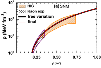
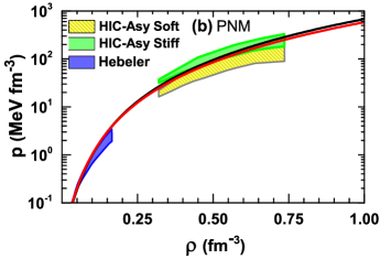
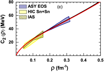
Figure 11: The pressure $P(\rho)$ for SNM (top), PNM (middle) and symmetry energy coefficient $C_{2}(\rho)$ (bottom) as a function of baryon density $\rho$ for the best-fit parameters obtained from free variation of all the parameters (black lines) and for the final values of the parameters (see Table 2) shown by the red line. The figure is taken from Ref. Malik2018a .

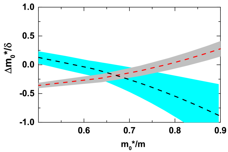
Figure 12: The isovector effective mass-splitting as a function of nucleon effective mass. The black dashed line refers to the best fit obtained from macrodata for different values of $\tilde{\alpha}$; the red dashed line corresponds to the one obtained by satisfying Eq. (57) with $\Theta_{v}=145$ MeV fm⁵. The cyan and grey shades refer to the respective uncertainties. The figure is taken from Ref. Malik2018a .

5 Message from the heavens

5.1 Neutron star properties: relations to symmetry elements

Neutron stars are incredibly dense objects, made of baryonic matter, mostly of neutrons. Matter at supra-nuclear densities, as encountered in the core of the neutron star can not be accessed in terrestrial experiments, astrophysical observations involving the neutron stars are thus essential in understanding dense matter EoS. The degenerate baryon pressure balances the gravitational pull preventing stars as heavy as of mass $\approx 2M_{\odot}$ from turning into black-holes. The so-far observed maximum mass of the neutron star with $M_{\rm NS}\approx 2M_{\odot}$ Antoniadis2013 ; Demorest2010 ; Rezzolla2018 ; Cromartie2019 thus serves as a stringent constraint on the nuclear matter EoS. This observation sets, till now, the absolute limit on the softness/stiffness of the EoS and helps in focussing on those EDFs that satisfy this observational criterion.

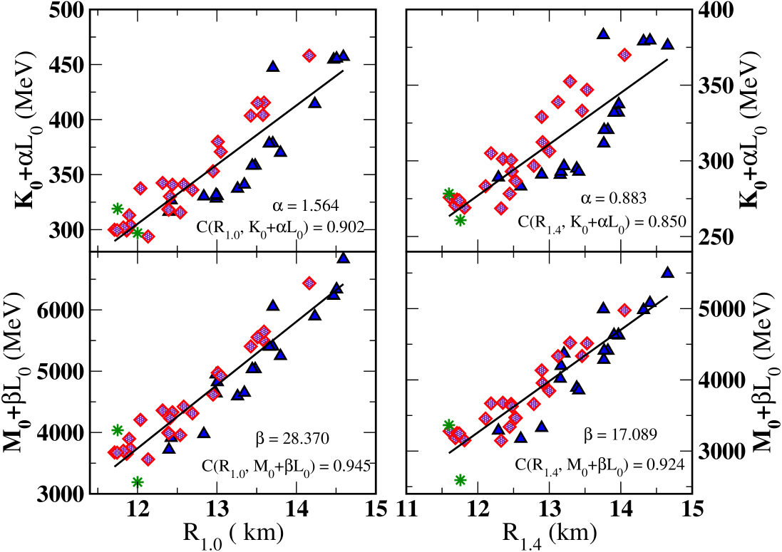
Figure 13: Neutron star radii $R_{1.0}$ (left) and $R_{1.4}$ (right) versus the linear correlations $K_{0}+\alpha L_{0}$ ( top ) and $M_{0}+\beta L_{0}$ (bottom), using a set of RMF (blue triangles), Skyrme (red diamonds), and BHF+APR (green stars) calculations. The figure is taken from Ref. Alam2016 .

Since, the EoS is determined, in principle, by Eqs. (2) and (3), the nuclear matter parameters entering the EoS should show some correlation with some properties of neutron star, such as the crust-core transition density and pressure, radii, maximum mass etc. As examples, the crust-core transition density is seen to be strongly correlated to the symmetry slope $L_{0}$ or the neutron skin of a heavy nucleus Vidana2009 ; Ducoin2010 , the transition pressure is found to be strongly correlated with a linear combination of $L_{0}$ and the symmetry curvature $K_{\rm sym}^{0}$ at a sub-nuclear density ($\rho\sim 0.1$ fm^-3) Ducoin2011 ; Newton2013 ; Fattoyev2014 . Such correlations point to some general interrelationships between the nuclear matter parameters and the properties of high density nuclear matter. They may only be useful in having a close understanding of a still largely unknown nuclear matter parameters when its interrelating partners are well known. For example, the simultaneous determination of mass and radius of a low mass neutron star has been shown to constrain better the product of nuclear matter incompressibility $K_{0}$ and the symmetry slope $L_{0}$Sotani2015 but till now, it appears, the NS radius or $L_{0}$ are not that well constrained; to be more specific, if the mass and radius of the low mass NS and $K_{0}$ are to be taken to the constrained values, the value of $L_{0}$ seems in present knowledge uncharacteristically large. It may not be hard to comprehend that low mass neutron stars ($\sim 0.6M_{\odot}$) may not involve too high core density for degenerate baryon pressure to support the gravitational pull; with that understanding, the radii of low mass neutron stars were correlated with the neutron skin of ²⁰⁸Pb (a manifestation of neutron pressure at $\sim\rho_{0}$ Fattoyev2010 ). However neutron star with such low mass are not yet discovered, the lowest NS mass observed so far is $1.17\pm 0.004M_{\odot}$ Martinez2015 . It was found that the correlation is extremely strong for low mass neutron stars, getting weaker as the mass of the neutron star increases. In the same vein, Alam et al Alam2016 investigate the correlation of neutron star radii with the key nuclear matter parameters governing the nuclear matter EoS; they find a correlation of the NS radii with $K_{0},M_{0},$ and $L_{0}$ but not strong enough to give a good understanding of the EoS. A linear combination of these nuclear matter parameters like $K_{0}+\alpha L_{0}$ and $M_{0}+\beta L_{0}$ with the NS radii give a better correlation, the correlation becoming stronger with lower masses of the neutron star (see Fig. 13). Though, the values of $L_{0}$ and $M_{0}$ are not very certain, their plausible values as deduced from finite nuclear data constrain the radius $R_{1.4}$ of a canonical star of mass $1.4M_{\odot}$ in the range 11.09 - 12.86 km.

5.2 Tidal deformability and relations to symmetry elements

In August 2017, the advanced LIGO and advanced VIRGO gravitational wave observatories detected gravitational waves (The GW170817 event) from merger of two neutron stars Abbott2017 . During the last stages of the inspiral motion of the coalescing neutron stars the strong gravity of each induces a strong tidal deformation in the companion star. The gravitational wave phase evolution caused by the deformation Flanagan2008 is decoded allowing for the determination of a dimensionless tidal deformability parameter $\Lambda$ Hinderer2008 ; Hinderer2010 ; Damour2012 . It measures the response of the gravitational pull on the surface of the neutron star and thus becomes the correlator of the pressure gradients inside the NS serving as an effective probe of the high density nuclear matter EoS Hawking1987 ; Read2009 . A relatively large value of $\Lambda$, for example, points to a relatively large neutron star radiusAnnala2018 ; De2018 ; Malik2018 ; that speaks of a stiff EoS and hence a comparatively large value of the neutron skin of a heavy nucleus Fattoyev2018 .

The tidal deformability parameter $\lambda$ is defined as Flanagan2008 ; Hinderer2008 ; Damour2012

$$Q_{ij}=-\lambda\mathcal{E}_{ij},$$ (59)

where $Q_{ij}$ is the induced quadrupole moment of a star in a binary due to the static external tidal field $\mathcal{E}_{ij}$ of the companion star. The parameter $\lambda$ can be expressed in terms of the dimensionless quadrupole tidal Love number $k_{2}$ as (we take the geometrized unit $G=c=1$),

$$\lambda=\frac{2}{3}k_{2}R^{5},$$ (60)

where $R$ is the radius of the NS. The value of $k_{2}$ depends on the stellar structure, it can be obtained Hinderer2008 ; Malik2018 in conjunction with solving for the Tolmann-Volkoff equations Weinberg1972 . Typically, the value of $k_{2}$ lies in the range $\approx 0.05-0.15$ Hinderer2008 ; Postnikov2010 for neutron stars. The dimensionless tidal deformability is then defined as $\Lambda=\frac{2}{3}k_{2}C^{-5}$ where $C(\equiv M/R)$ is the compactness of the star of mass $M$. The Love number $k_{2}$ has a veiled NS radius dependence: Ref. De2018 finds $\Lambda\sim R^{6}$, Ref. Tsang2019 finds it as $\sim R^{6.26}$ while in Ref. Malik2018 , for a NS of canonical mass $1.4M_{\odot}$, it is $\sim R^{6.13}$. There is thus expected a strong correlation between $\Lambda$ and $R$. The tidal deformabilities of the neutron stars present in the binary system can be combined to yield an weighted average as

$$\tilde{\Lambda}=\frac{16}{13}\frac{(12q+1)\Lambda_{1}+(12+q)q^{4}\Lambda_{2}}{(1+q)^{5}},$$ (61)

where $\Lambda_{1,2}$ are the tidal deformabilities of the NSs of mass $M_{1}$ and $M_{2}$ and $q=M_{2}/M_{1}\leq 1$ is the binary’s mass ratio. Early analysis of the GW170817 event Abbott2017 puts an upper limit for $\tilde{\Lambda}$ at $\approx 800$ for the component neutron stars with masses in the range $\approx 1.17M_{\odot}-1.6M_{\odot}$ involved in the merger event. Revised values of $\tilde{\Lambda}$ seem to be substantially lower De2018 ; Abbott2018 ; Abbott2019 . With a few plausible assumptions for a canonical neutron star, a restrictive constraint has been set for $\Lambda_{1.4}$ to $\sim 190^{+390}_{-120}$ Abbott2018 . From the spectral parameterization of the pressure $P(\rho)$ for the $\beta$-equilibrated matter to fit the observational template, the pressure inside the NS at supra-normal densities is also predicted. The goal now remains to be seen: to find the most realistic EoS that connects all the constraints involving microscopic nuclei with those obtained from astrophysical scenario, namely, the maximum neutron star mass and the tidal deformability.

Initial attempts in this direction have been made on understanding the sensitivity of the tidal deformability to the nuclear matter parameters related to nuclear matter at saturation density. In Ref. Malik2018 , the correlation of $\Lambda,k_{2}$ and $R$ with the nuclear matter parameters $K_{0},Q_{0},M_{0},C_{2}^{0},L_{0},K_{\rm sym}^{0}$ and with several linear combinations of two parameters, in particular, $K_{0}+\alpha L_{0},M_{0}+\beta L_{0}$ and $M_{0}+\eta K_{\rm sym}^{0}$ are studied with a set of 18 relativistic and 24 non-relativistic nuclear models that are known to yield a good description of the properties of finite nuclei and neutron stars. The correlation systematics is determined for NS masses in the range $1.2M_{\odot}-1.6M_{\odot}$, since for analysis of low spin prior as assumed in Ref. Abbott2017 , these masses are close to the GW170817 event. Calculations in Ref. Malik2018 show that the individual nuclear matter parameters are weakly or moderately correlated with $\Lambda,k_{2}$ and $R$, but $\Lambda$ and $R$ have tight correlation with $M_{0}+\beta L_{0}$ and $M_{0}+\eta K_{\rm sym}^{0}$ over a wide range of NS masses considered; the correlation coefficient $r$ is $\sim 0.9$. The Love number $k_{2}$ is, however, only strongly correlated with $M_{0}+\eta K_{\rm sym}^{0}(r\sim 0.92)$. The values of $\alpha,\beta$ and $\eta$ are obtained from the demand of optimum correlations for each NS mass; they are found to decrease monotonically with increase in NS mass. This indicates that the density dependence of the symmetry energy is less important in determining the tidal deformability and the radius at higher NS masses. Representative examples of the fit of $M_{0}+\beta L_{0}$ and $M_{0}+\eta K_{\rm sym}^{0}$ with $\Lambda_{1.4}$ are shown in Fig. 14. The figure shows that once $\Lambda_{1.4}$ and $L_{0}$ are known within tight limits, $M_{0}$ can be constrained and then $K_{\rm sym}^{0}$. Empirical values of $M_{0}$ and $K_{\rm sym}^{0}$ derived for different limits of $\Lambda_{1.4}$ and $L_{0}$ are shown in Table 4. On the other end, the strong correlation of $\Lambda_{1.4}$ with $R_{1.4}$ mentioned earlier puts a strong constraint on the radius of a canonical neutron star that can be compared to that obtained from the simultaneous determination of the radius and mass of a NS with the NICER (Neutron star Interior Composition Explorer) mission Riley2019 ; Raaijmakers2019 ; Miller2019 . To further the understanding of the relationship of the tidal deformability to the isovector nuclear matter parameters, Tsang et. al Tsang2019 studied, with a total of 240 Skyrme interactions the correlation of $\Lambda$ with $C_{2}^{0},~{}L_{0},~{}K_{\rm sym}^{0}$ and $Q_{\rm sym}^{0}$; they found little correlation except between $\Lambda-L_{0}$ and $\Lambda-K_{\rm sym}^{0}$, the later one being the strongest as displayed in Fig.15. In Ref.Zhang2018 , a stronger correlation between $\Lambda$ and $L_{0}$ than between $\Lambda$ and $K_{\rm sym}^{0}$ is reported; this has to be critically examined further as one expects the opposite since $K_{\rm sym}^{0}$ impacts higher densities more.

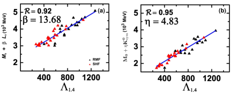
Figure 14: (a) The $M_{0}+\beta L_{0}$ and (b) $M_{0}+\eta K_{\rm sym}^{0}$ versus the dimensionless tidal deformability $\Lambda_{1.4}$ for a $1.4~{}{\rm M}_{\odot}$ NS, using a set of RMF and SHF models. The figure is taken from Ref. Malik2018 .

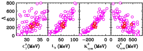
Figure 15: The four panels show the correlation between the tidal deformability of neutron star$\Lambda$ for 1.4 solar-mass neutron stars and Taylor expansion coefficients (from left to right) $C_{2}^{0},L_{0},K_{\rm{\rm sym}}^{0}{\rm and~{}}Q_{\rm{\rm sym}}^{0}$ defined in Eq. 3 obtained for the Skyrme functionals used in Ref. (Tsang2019 ). The figure is taken from Ref. Tsang2019

To avoid model dependence on the results of correlations between nuclear matter parameters and the NS properties and to look for further correlations, an approach taken in several works De2015 ; Margueron2018a ; Margueron2019 termed ’meta-modelling’ has been applied recently Ferreira2020 to construct the nuclear matter EoS. Based on the Taylor expansion of the energy functional around the saturation density (as shown in Eqs.2 and 3), with expansion coefficients identified as different nuclear matter parameters, the EoS in principle, is model-independent provided the nuclear matter parameters are experimentally known. Exploiting the idea, in Ref. Ferreira2020 , millions of EOSs are constructed with the eight nuclear matter parameters ($K_{0}$, $Q_{0}$, $Z_{0}$, $C_{2}^{0}$, $L_{0}$, $K_{\rm sym}^{0}$, $Q_{\rm sym}^{0}$, $Z_{\rm sym}^{0}$) each one having a Gaussian distribution around the supposedly known central values. The multivariate Gaussian is taken to have zero covariance. The saturation energy and density are fixed at $e_{0}=-15.8$ MeV and $\rho_{0}$ = 0.155 fm^-3. Out of the million EoSs so generated only $\sim$ 2000 are selected to be valid ones filtered from imposition of the following constraints: (i) the EoS must be thermodynamically stable (ii) it should be causal, (iii) should support the observational constraint of the maximum mass at least as high as 1.97 $M_{\odot}$, (iv) the tidal deformability should be $70<\Lambda_{1.4}<580$ Abbott2017 and (v) the symmetry energy $C_{2}(\rho)$ should be positive. All the EoSs are obtained for the matter composed of neutrons, protons, electrons and muons in $\beta$-equilibrium. The low density part ($\rho<0.1$ fm^-3) of the EoSs are matched with the SLy4 EoS so that $P_{SLy4}(\mu)=P_{EoS}(\mu)$ where $\mu$ is the chemical potential.

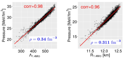
Figure 16: $\Lambda_{1.4M_{\odot}}$ (left) and $R_{1.4M_{\odot}}$ (right) as a function of the pressure for all meta models used in Ref. Ferreira2020 at the densities corresponding to the maximum correlations. These densities and correlation coefficients are indicated in each of the panels. The figure is taken from Ferreira2020 .

The filtered EoSs are employed to calculate the mass ($M$) radius ($R$) and the tidal deformability ($\Lambda$) of neutron stars and then to study the possible existing correlations between the NS observables and the thermodynamic properties of dense stellar matter in $\beta$-equilibrium. Strong correlations between them are found to build up at different densities depending on the NS masses, for example, correlation between $P(\rho)$ for $\beta$-equilibrated matter and $R_{M}$ (radius of NS of mass M) is found to be almost unity at $\rho\sim 0.2$ fm^-3 for NS mass of 1.0 $M_{\odot}$; this peak value shifts to $\sim\rho=0.35$ fm^-3 when the NS mass is 1.6$M_{\odot}$. A similar correlation is observed between $P(\rho)$ and $\Lambda_{M}$ in the same range of densities. Strong correlations are also identified between the energy density $\mathcal{E}(\rho)$ with all the NS observables, but at larger densities, $\rho\simeq 0.32-0.5$ fm^-3, the smaller NS masses corresponding to smaller densities. The strong correlation $r\sim 1.0$ can be used as a tool to constrain thermodynamic quantities at different densities from the NS observables. For example, correlations between $P$ and $\Lambda$ and between $P$ and $R$ for NS mass 1.4$M_{\odot}$ are shown in the left and right panels of Fig. 16.

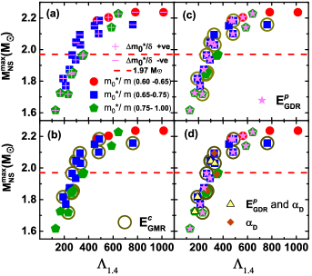
Figure 17: The maximum neutron star mass $M_{\rm NS}^{\rm max}$ versus the tidal deformability parameter $\Lambda_{1.4}$ obtained from the 28 selected EDFs. The red dashed lines refer to $1.97M_{\odot}$, the observed lower bound for $M_{\rm NS}^{\rm max}$ . For more details , see Ref. Malik2019 . The figure is borrowed from Ref. Malik2019 .

In both cases, the correlation is found to be very strong at $\rho\sim 0.32$ fm^-3 . If a simultaneous precise measurement of the mass and radius of NS is possible, say with the NICER mission, then from the radius, a constraint on the pressure of the $\beta$ stable stellar matter can be obtained at $\rho\sim 0.32$ fm^-3. This in turn gives an idea about $\Lambda_{1.4}$. In passing we note that in Ref. Ferreira2020 , correlations between the energy density $\mathcal{E}$ and sound velocity in stellar matter with $\Lambda_{1.4}$ and $R_{1.4}$, respectively, were also observed, but at somewhat different densities. A single determination $\Lambda_{M}$ or radius $R_{M}$ of a NS of mass $M$ thus allows to constrain the thermodynamical properties at three different distinct but close densities.

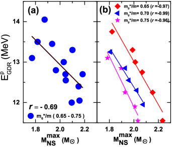
Figure 18: Correlation of $E_{\rm GDR}^{\rm p}$ and $M_{\rm NS}^{\rm max}$ obtained using (a) the set of selected models as in Fig. 17 with effective mass $m^{*}_{0}/m$ in the range 0.65 -0.75 and (b) a set of systematically varied models with chosen fixed effective masses in the present work. The figure is taken from Ref. Malik2019 .

5.3 In tandem with micro-physics: proposing a new EoS

The laudatory approach taken in the meta-modeling of the EoS serves as a guide to reach to probable values of the thermodynamical variables at different densities. Its success, however, depends on the precision choice of the input nuclear matter parameters. They may not be beyond question. The truncation order (see Eqs. (2) and (3)) or the size of the parameter space may also deem to be a suspect, particularly, at very low densities $\leq 0.5\rho_{0}$ and at very high densities, relevant to massive neutron stars Ferreira2020 . However, the efficacy of the EoS in matching many details of microscopic nuclear physics in tandem with astrophysical observations has not yet been soundly checked, even if the few input nuclear matter parameters entering the meta-modeling might be consistent.

Close inspection of nuclear matter EoS shows that it must be stiff enough to support a NS mass of $\sim 2M_{\odot}$, but soft enough so that $\Lambda_{1.4}<580$ Abbott2017 . Attempts have been made to establish a connection between the tidal deformability and microscopic nuclear physics from different ends, from sophisticated microscopic modeling of the low density EoS in chiral effective field theory (CEFT) Tews2018 ; Lim2018 ; Tews2019 ; Lim2019 or from use of a RMF inspired family of EoS models calibrated to provide a good description of a set of finite nuclear properties Fattoyev2018 . The somewhat ambivalent outcomes give the realization that the connection of $\Lambda$ to the laboratory data is not yet fully transparent and that more stringent constraints on the isovector sector of the effective interaction are needed.

The robust correlations of $\Lambda_{1.4}$ and $R_{1.4}$ with selective linear combinations of isoscalar and isovector properties of nuclear matter Malik2018 throw a strong hint that the isovector giant resonances in conjunction with the isoscalar resonances in finite nuclei may help in guiding to such strong constraints. To have a deeper look into these nuances of microscopic nuclear physics, Malik et al Malik2019 chose to study few experimental data of particular interest involving isoscalar and isovector properties of finite nuclei, namely, (i) the centroid energy $E_{\scriptsize{GMR}}$ of isoscalar giant monopole resonance (ISGMR), (ii) the peak energy $E_{GDR}^{p}$ of the isovector giant dipole resonance (IVGDR), and (iii) the dipole polarizability $\alpha_{D}$, all for the heavy nucleus ²⁰⁸Pb, corroborated with results from astrophysical sector, namely, the maximum mass of a NS and the tidal deformability. The analysis was done in the Skyrme framework with twenty-eight chosen ’best’ accepted Skyrme EDFs. These EDFs provided a satisfactory reproduction of the binding energies of finite nuclei and their charge radii, and obeyed reasonable constraints on the saturation density ($\rho_{0}=0.16\pm 0.01$ fm^-3), binding energy ($e_{0}=-15.8\pm 0.5$ MeV), isoscalar nucleon effective mass ($m_{0}^{*}/m=0.60-1.00$) and the isoscalar nuclear matter incompressibility ($K_{0}=240\pm 30$ MeV). The results, displayed in Fig. 17, with the maximum mass of a NS $M_{\rm max}$ plotted against $\Lambda_{1.4}$ are self explanatory with the symbols marked there. They show that only 3 of the 28 EDFs satisfy all the constraints imposed from finite nuclei and astrophysical data. Commensurate with the constraint on the maximum mass of a NS ($M_{\rm max}\sim 2.0M_{\odot}$), the tidal deformability for a canonical star comes out to be $\Lambda_{1.4}\sim 290-330$, the effective mass $m_{0}^{*}/m\sim 0.7$ and the isovector mass splitting $\Delta m_{0}^{*}\sim-0.2\delta$. The essence of the survey is that fulfilling simultaneously isoscalar and isovector constraints with the astrophysical ones is extremely restrictive.

The conclusion drawn from Fig. 17 on the tidal deformability $\Lambda_{1.4}$ is indicative of the domain in which its value may lie. To have a more quantitative assessment on it, a new EoS , albeit in the Skyrme framework, has been proposed Malik2019 with a wider fit data base. These constraints include the observed maximum NS mass, the binding energies of spherical magic nuclei, their charge radii, the ISGMR energies of ⁹⁰Zr, ¹²⁰Sn and ²⁰⁸Pb and the dipole polarizability $\alpha_{D}$ of ⁴⁸Ca, ⁶⁸Ni, ¹²⁰Sn and ²⁰⁸Pb. The IVGDR peak energies are left out of the fitting protocol deliberately. Simultaneously constraining all data impose severe restrictions on the model parameters. As example, calculations with the selected EDFs of Fig. 17 reveal the existence of some anti-correlation ($r\sim-0.69$) of $E_{GDR}^{p}$ (²⁰⁸Pb) with $M_{\rm max}$ when the EDFs are sorted out in groups within narrow windows of $m_{0}^{*}/m$ (see panel (a) of Fig. 18). This correlation shoots up to nearly unity ($r\sim 1.0$) when calculated with systematically varied models with fixed values of $m_{0}^{*}/m$ as displayed in panel (b) of the same figure. For given values of $M_{\rm max}$ and $m_{0}^{*}/m$, $E_{GDR}^{p}$ is the outcome of the calculation keeping all other data in the fitting protocol unchanged.

Looking at the trends depicted by Figs. 17 and 18, it is evident that the values of $\Lambda_{1.4}$ is sensitive to the maximum neutron mass as well as various ground and excited state properties of the finite nuclei. The optimized $\chi^{2}$ -function obtained by fitting these data yields the EDF parameters as listed in Table 5 Malik2019 . The errors on the parameters are calculated within the covariance method Zhang2018a ; Dobaczewski2014 . The central value of $\Lambda_{1.4}$ comes out to be 267; we call this EDF SK$\Lambda$267. With this EDF it is seen that all the nuclear matter parameters and the lower limit on $M_{\rm max}$ are in comfortably acceptable bounds; $\Lambda_{1.4}$ and $R_{1.4}$ are seen to be in very good agreement with those reported recently Sabatucci2020 ; Bonnard2020 . The value of $M_{\rm max}$ is (2.04$\pm$0.15)$M_{\odot}$, that of the neutron skin $\Delta r_{np}$ for ²⁰⁸Pb is $0.15\pm 0.05$ fm.

The experimental value of tidal deformability is not settled yet, we therefore test the tolerance of the fit of the calculated observables with data by arbitrarily constraining $\Lambda_{1.4}$ to different values. As example, an extra constraint $\Lambda_{1.4}=500\pm 100$ was used in the fit. The outcome is $\Lambda_{1.4}=484\pm 215$, with somewhat different Skyrme parameters. This EoS, is called SK$\Lambda$484 Malik2019 is somewhat stiffer than SK$\Lambda$267. As expected, it produces a larger $R_{1.4}$ 13.1$\pm$1.4 km compared to 11.6$\pm$1.0 km for a canonical NS, a larger $\Delta r_{np}$ 0.21$\pm$0.04 fm for ²⁰⁸Pb and a somewhat larger $M_{\rm max}$ 2.10$\pm$ 0.04 $M_{\odot}$. The isoscalar nuclear matter parameters like $e_{0},K_{0},Q_{0}$ or $m_{0}^{*}$ are nearly unaffected, but the isovector parameters suffer some changes. Overall, it appears , the softer model SK$\Lambda$267 is more compatible with the measured properties of finite nuclei.

Table 1: List of fit data corresponding to the symmetric nuclear matter (SNM), pure neutron matter (PNM) and symmetry energy coefficient (SYM) together with the range of densities in which they are determined. Here $P(\rho)$ represents pressure of nuclear matter, ${e}_{n}(\rho)$ is the energy per neutron in PNM and $C_{2}(\rho)$ is the symmetry energy coefficient.

	Quantity	Density region	Band/Range	Ref.
		fm-3	(MeV)
SNM	$P(\rho)$	$0.32~{}{\rm to}~{}0.74$	HIC	Danielewicz2002
SNM	$P(\rho)$	$0.19~{}{\rm to}~{}0.33$	Kaon exp	Fuchs2006 ; Fantina2014
PNM	${e}_{n}(\rho)$	0.1	$10.9\pm 0.5$	Brown2013
PNM	${e}_{n}(\rho)$	$0.03~{}{\rm to}~{}0.17$	N3LO	Hebeler2013
PNM	$P(\rho)$	$0.32~{}{\rm to}~{}0.73$	HIC	Danielewicz2002
PNM	$P(\rho)$	$0.03~{}{\rm to}~{}0.17$	N3LO	Hebeler2013
SYM	$C_{2}(\rho)$	0.1	$24.1\pm 0.8$	Trippa2008
SYM	$C_{2}(\rho)$	$0.01~{}{\rm to}~{}0.19$	IAS,HIC	Danielewicz2014 ; Tsang2009
SYM	$C_{2}(\rho)$	$0.01~{}{\rm to}~{}0.31$	ASY-EoS	Russotto2016

Table 2: The final model parameters obtained by optimizing the $\chi^{2}$ function together with the uncorrelated and correlated errors (see text for details). The parameters $K_{1}$ and $K_{2}$ are in units of MeV.fm^-3, $a$ and $b$ are in MeV and $k_{+}$ and $k_{-}$ are in fm³.

${\tilde{\alpha}}$	$K_{1}$	$K_{2}$	$a$	$b$	$k_{+}$	$k_{-}$
1.11	-1220.21	977.94	120.03	-121.93	6.07	2.60
Unc. err.	1.16	2.38	0.15	0.33	0.10	0.15
Cor. err.	103.04	90.25	15.01	13.57	1.13	0.96

Table 3: Different properties pertaining to nuclear matter (NM) and neutron star (NS) obtained with the final parameters listed in Table 2. $K_{\tau}$ is the symmetry incompressibility at saturation density corresponding to ANM: it is defined as $K_{\tau}=K_{\rm sym}^{0}-6L_{0}-Q_{0}L_{0}/K_{0}$

Type		Unit	Value
NM	$e_{0}$	MeV	$-15.93\pm 0.20$
	$\rho_{0}$	fm-3	$0.1620\pm 0.003$
	$K_{0}$	MeV	$225.23\pm 6.50$
	$m_{0}^{*}/m$		$0.67\pm 0.04$
	${m_{v,0}^{*}}/{m}$		$0.78\pm^{0.05}_{0.04}$
	$\Delta m_{0}^{*}/\delta$		$-0.19\pm 0.08$
	$C_{2}(\rho_{0})$	MeV	$33.94\pm 0.50$
	$L_{0}$	MeV	$68.50\pm 3.74$
	$K_{\rm sym}^{0}$	MeV	$-47.46\pm 17.28$
	$K_{\tau}$	MeV	$-349.22\pm 13.19$
	$M_{\rm c}$	MeV	$998.79\pm 41.38$
	$Q_{0}$	MeV	$-359.23\pm 23.82$
NS	$M_{\rm max}^{\rm NS}$	$M_{\odot}$	$2.07\pm 0.03$
	$R_{1.4}$	km	$12.63\pm 0.17$

Table 4: The empirical values of $M_{0}$ and $K_{\rm sym}^{0}$ derived for different limits on $\Lambda_{1.4}$ and $L_{0}$. The value of $\Lambda<800(400)$ is derived with 90%(50%) confidence limit for GW170817. The ranges of $L_{0}=30-86$ MeV and $40-62$ MeV are taken from references Oertel2017 ; Lattimer2013 . The value of $K_{\rm sym}^{0}$ has a good overlap with that obtained recently Zimmerman2020 from NICER and LIGO/VIRGO constraints.

$L_{0}$	$\Lambda_{1.4}$	$M_{0}$	$K_{\rm sym}^{0}$
(MeV)		(MeV)	(MeV)
30 – 86	0 – 800	1972 – 2878	-143.8 – 19.8
	0 – 400	1972 – 2042	-143.8 – 17.3
40 – 62	0 – 800	1836 – 3206	-115.5 – -48.2
	0 – 400	1836 – 2371	-115.5 – -50.7

Table 5: Parameters for the model Sk$\Lambda$267 and the resulting nuclear matter and neutron star properties along with their errors in the parenthesis. $C_{2}^{0}$ is the symmetry energy coefficient, $L_{0}$ is related to its density derivative Malik2018a .

$t_{0}$	$t_{1}$	$t_{2}$	$t_{3}$	$x_{0}$	$x_{1}$	$x_{2}$	$x_{3}$	$\alpha$	$W_{0}$
( MeVfm3 )	( MeVfm5 )	( MeVfm5 )	( MeVfm3+3α )						( MeVfm5 )
-2481.08	482.51	-516.17	13778.74	0.93	-0.53	-0.97	1.54	0.167	121.38
(89.05)	(50.41)	(407.22)	(123.72)	(0.28)	(0.89)	(0.20)	(0.58)	(0.018)	(9.35)
$e_{0}$	$\rho_{0}$	$K_{0}$	$m_{0}^{*}/m$	$C_{2}^{0}$	$L_{0}$	$\Delta m_{0}^{*}/\delta$	$\Lambda_{1.4}$	$R_{1.4}$	$M_{\rm NS}^{\rm max}$
(MeV)	(fm${}^{-3})$	(MeV)		(MeV)	(MeV)			(km)	($M_{\odot}$)
$16.04$	0.162	230.2	0.70	31.4	41.1	-0.25	267	11.6	2.04
( 0.20 )	(0.002)	(6.4)	(0.05)	( 3.1)	( 18.2)	(0.35)	(144)	( 1.0)	(0.15)

Table 6: The constraints on isoscalar and isovector nuclear matter parameters together with radius and tidal deformability of neutron star with canonical mass and the neutron-skin thickness in ²⁰⁸Pb nucleus derived from microscopic and macroscopic data in the present work. The isoscalar parameters considered are the nuclear matter incompressibility coefficient $K_{0}$, skewness parameter $Q_{0}$ and nucleon effective mass $m_{0}^{*}$ and those corresponding to the isovector sector are the symmetry energy coefficient $C_{2}^{0}$, slope $L_{0}$, curvature $K_{\rm sym}^{0}$ and skewness $Q_{\rm sym}^{0}$ and the effective nucleon mass splitting $\Delta m_{0}^{*}/\delta$.

Quantity		Unit	Values from Refs.
			Mondal2017	Malik2018a	Malik2019	RocaMaza2013a	De2015	Agrawal2012 ; Agrawal2013
SNM	$K_{0}$	MeV		$225.0\pm 6.4$	$230.0\pm 6.4$		$212.0\pm 20.1$
	$Q_{0}$			$-359.0\pm 23.0$	$-367.0\pm 12.0$		$-378.0\pm 31.6$
	$m_{0}^{\star}/m$	-	$0.7\pm 0.1$	$0.68\pm 0.04$	$0.70\pm 0.05$
ANM	$C_{2}^{0}$	MeV	$32.1\pm 0.31$	$33.94\pm 0.5$	$31.4\pm 3.1$	$31\pm 2_{\rm est}$
	$L_{0}$		$60.3\pm 14.5$	$68.5\pm 3.74$	$41.1\pm 18.2$	$43\pm 6_{\rm exp}\pm 8_{\rm the}\pm 12_{\rm est}$		$59.3\pm 12.8$
	$K_{\rm sym,0}$		$-111.8\pm 71.3$	$-47.46\pm 17.28$	$-123.9\pm 70.2$
	$Q_{\rm sym,0}$		$296.8\pm 73.6$	$394.07\pm 24.96$	$564.63\pm 98.73$
	$\Delta m_{0}^{\star}/\delta$	-	$0.17\pm 0.24$	$-0.19\pm 0.08$	$0.25\pm 0.35$
208 Pb	$\Delta r_{np}$	fm						$0.195\pm 0.022$
NS	$R_{1.4}$	km		$12.63\pm 0.17$	$11.6\pm 1.0$
	$\Lambda_{1.4}$	-			$267\pm 144$

In Table 6, we collect the values of various isoscalar and isovector nuclear matter parameters constrained by microscopic and macroscopic data considered in the present work. We also provide the constraints on the radius and tidal deformability for the neutron star with the canonical mass and the neutron-skin thickness in the ²⁰⁸Pb nucleus. This table is far from being complete and may be complemented with the constraints provided recently, for instance Ref. RocaMaza2018 . The splitting of effective nucleon mass are found to be positive as well as negative. The negative values are obtained only when the electric dipole polarizability in nuclei and the maximum mass of the neutron star are constrained simultaneously. The values of $L_{0}$ and $\Delta r_{np}$ presented in the last column of the table are obtained by combining the results from three different ansatz for the density dependence of the symmetry energy. The best fit estimates for radius and the mass of the PSR J0030+0451 obtained by NICER are $R=13.02^{+1.24}_{-1.06}$ km for the $M_{\rm NS}=1.44^{+0.15}_{-0.14}M_{\odot}$ Miller2019 . These values have good overlap with the ones presented in the Table 6. More precise values of these quantities are , however, required to constrain the nuclear matter parameters and the EOS.

6 Summary and Outlook

All the rich physics of the interacting nucleons is telescopically encoded in the nuclear matter parameters; a model-independent EoS of symmetric and asymmetric nuclear matter can be built on them. A convenient means to link these parameters to the properties of finite nuclei and of neutron stars is provided by the nuclear mean-field models. The parameters such as the binding energy per nucleon, the saturation density, the nuclear matter incompressibility coefficient and symmetry energy coefficient have been determined within a narrow window from the ground state and excited state properties of finite nuclei, the higher order density derivatives such as the density slope of symmetry energy or the skewness parameter are still not known in comparative precision. Attempts have been made in the last few years to contain them in narrow bounds through correlation analysis, we review them in this article. The Skyrme mean-field approach, till date has proved to be the most comprehensive in explaining diverse nuclear data, the review places more emphasis on it.

The nuclear matter parameters reflect different properties of nuclear matter, but they may be correlated to each other being the underpinnings of the varied aspects of the same nucleonic interactions. We have explored this correlation property analytically in the mean-field approach. The better known low order density derivatives help in narrowing down the uncertainty in the higher order derivatives. Additional information comes from the correlations of selective nuclear matter parameters with selective nuclear observables. For example, the symmetry density slope is sensitive to the neutron-skin of a finite nucleus as well as to the radii and the tidal deformability of neutron stars. Neutron star properties have been seen to be particularly sensitive to the higher order nuclear matter parameters. Present state of art technology, however, has not been able to contain the data emanating from neutron stars in more tight bounds. We hope, from the NICER mission and from the future advanced LIGO-VIRGO detection of gravitational waves, the cosmic data may find more fine resolution and their consonance with laboratory micro-physics may guide to a better understanding of the nuclear matter equation of state.

Acknowledgments

The authors acknowledge the the contribution of many collaborators, who over many years were instrumental in helping to develop the ideas that we threaded in this review. The authors are extremely thankful to Tanuja Agrawal for her assistance in the preparation of the manuscript. T. M. acknowledges the hospitality extended to him by Saha Institute of Nuclear Physics during the course of this work. J. N. D. acknowledges support from the Department of Science and Technology, Government of India with grant no. EMR/2016/001512.

References

- (1) W.D. Myers, W.J. Swiatecki, Annals Phys. 55, 395 (1969)
- (2) W.D. Myers, W.J. Swiatecki, Nucl. Phys. A336, 267 (1980)
- (3) P. Möller, W.D. Myers, H. Sagawa, S. Yoshida, Phys. Rev. Lett. 108(5), 052501 (2012)
- (4) J.P. Blaizot, Phys. Rept. 64, 171 (1980)
- (5) Y.W. Lui, D.H. Youngblood, Y. Tokimoto, H.L. Clark, B. John, Phys. Rev. C70, 014307 (2004)
- (6) T. Li, et al., Phys. Rev. Lett. 99, 162503 (2007)
- (7) U. Garg, Nucl. Phys. A788, 36 (2007)
- (8) T. Li, et al., Phys. Rev. C81, 034309 (2010)
- (9) D. Patel, et al., Phys. Lett. B718, 447 (2012)
- (10) E. Khan, J. Margueron, G. Colo, K. Hagino, H. Sagawa, Phys. Rev. C82, 024322 (2010)
- (11) E. Khan, J. Margueron, Phys. Rev. Lett. 109, 092501 (2012)
- (12) E. Khan, J. Margueron, Phys. Rev. C88(3), 034319 (2013)
- (13) J.N. De, S.K. Samaddar, B.K. Agrawal, Phys. Rev. C92(1), 014304 (2015)
- (14) X. Roca-Maza, N. Paar, Prog. Part. Nucl. Phys. 101, 96 (2018)
- (15) H. Jiang, G.J. Fu, Y.M. Zhao, A. Arima, Phys. Rev. C85, 024301 (2012)
- (16) L. Trippa, G. Colo, E. Vigezzi, Phys. Rev. C77, 061304 (2008)
- (17) X. Roca-Maza, M. Brenna, B.K. Agrawal, P.F. Bortignon, G. Colò, L.G. Cao, N. Paar, D. Vretenar, Phys. Rev. C87(3), 034301 (2013)
- (18) B.A. Brown, Phys. Rev. Lett. 85, 5296 (2000)
- (19) S. Typel, B.A. Brown, Phys. Rev. C64(2), 027302 (2001)
- (20) M. Centelles, X. Roca-Maza, X. Vinas, M. Warda, Phys. Rev. Lett. 102, 122502 (2009)
- (21) M. Warda, X. Vinas, X. Roca-Maza, M. Centelles, Phys. Rev. C80, 024316 (2009)
- (22) S. Abrahamyan, Z. Ahmed, H. Albataineh, K. Aniol, D.S. Armstrong, W. Armstrong, T. Averett, B. Babineau, A. Barbieri, Bellini, et al., Phys. Rev. Lett. 108, 112502 (2012). URL https://link.aps.org/OPTdoi/10.1103/PhysRevLett.108.112502
- (23) A. Carbone, G. Colo, A. Bracco, L.G. Cao, P.F. Bortignon, F. Camera, O. Wieland, Phys. Rev. C81, 041301 (2010)
- (24) M.A. Famiano, T. Liu, W.G. Lynch, A.M. Rogers, M.B. Tsang, M.S. Wallace, R.J. Charity, S. Komarov, D.G. Sarantites, L.G. Sobotka, Phys. Rev. Lett. 97, 052701 (2006)
- (25) B.K. Agrawal, J.N. De, S.K. Samaddar, Phys. Rev. Lett. 109, 262501 (2012)
- (26) B.K. Agrawal, J.N. De, S.K. Samaddar, G. Colo, A. Sulaksono, Phys. Rev. C87(5), 051306 (2013)
- (27) A.W. Steiner, S. Gandolfi, Phys. Rev. Lett. 108, 081102 (2012)
- (28) C. Mondal, B.K. Agrawal, J.N. De, Phys. Rev. C92(2), 024302 (2015)
- (29) N. Paar, C.C. Moustakidis, T. Marketin, D. Vretenar, G.A. Lalazissis, Phys. Rev. C90(1), 011304 (2014)
- (30) C.J. Horowitz, J. Piekarewicz, Phys. Rev. Lett. 86, 5647 (2001)
- (31) C. Ducoin, J. Margueron, C. Providencia, I. Vidana, Phys. Rev. C83, 045810 (2011)
- (32) X. Roca-Maza, X. Viñas, M. Centelles, B.K. Agrawal, G. Colo’, N. Paar, J. Piekarewicz, D. Vretenar, Phys. Rev. C92, 064304 (2015)
- (33) S. Teukolsky, S. Shapiro, (Wiley, 1983)
- (34) D. Kobyakov, C.J. Pethick, Phys. Rev. Lett. 112(11), 112504 (2014)
- (35) C.P. Lorenz, D.G. Ravenhall, C.J. Pethick, Phys. Rev. Lett. 70, 379 (1993)
- (36) D.K. Berry, M.E. Caplan, C.J. Horowitz, G. Huber, A.S. Schneider, Phys. Rev. C94(5), 055801 (2016)
- (37) K. Madhuri, D.N. Basu, T.R. Routray, S.P. Pattnaik, Eur. Phys. J. A53(7), 151 (2017)
- (38) A. Guerra Chaves, T. Hinderer, J. Phys. G46(12), 123002 (2019)
- (39) G. Baym, C. Pethick, P. Sutherland, Astrophys. J. 170, 299 (1971)
- (40) P. Danielewicz, R. Lacey, W.G. Lynch, Science 298, 1592 (2002)
- (41) C. Fuchs, Prog. Part. Nucl. Phys. 56, 1 (2006)
- (42) A.F. Fantina, N. Chamel, J.M. Pearson, S. Goriely, EPJ Web Conf. 66, 07005 (2014)
- (43) B.P. Abbott, et al., Phys. Rev. Lett. 119(16), 161101 (2017)
- (44) T. Malik, N. Alam, M. Fortin, C. Providência, B.K. Agrawal, T.K. Jha, B. Kumar, S.K. Patra, Phys. Rev. C98(3), 035804 (2018)
- (45) T. Malik, B.K. Agrawal, J.N. De, S.K. Samaddar, C. Providência, C. Mondal, T.K. Jha, Phys. Rev. C99(5), 052801 (2019)
- (46) M.B. Tsang, W.G. Lynch, P. Danielewicz, C.Y. Tsang, Phys. Lett. B795, 533 (2019)
- (47) A. Ekström, (2019)
- (48) R. Machleidt, Phys. Rev. C63, 024001 (2001)
- (49) D.R. Entem, R. Machleidt, Phys. Rev. C68, 041001 (2003)
- (50) U. van Kolck, Prog. Part. Nucl. Phys. 43, 337 (1999)
- (51) E. Epelbaum, H.W. Hammer, U.G. Meissner, Rev. Mod. Phys. 81, 1773 (2009)
- (52) R. Machleidt, D.R. Entem, Phys. Rept. 503, 1 (2011)
- (53) D. Lee, Prog. Part. Nucl. Phys. 63, 117 (2009)
- (54) B.R. Barrett, P. Navratil, J.P. Vary, Prog. Part. Nucl. Phys. 69, 131 (2013)
- (55) A. Carbone, A. Cipollone, C. Barbieri, A. Rios, A. Polls, Phys. Rev. C88(5), 054326 (2013)
- (56) G. Hagen, T. Papenbrock, M. Hjorth-Jensen, D.J. Dean, Rept. Prog. Phys. 77(9), 096302 (2014)
- (57) H. Hergert, S.K. Bogner, T.D. Morris, A. Schwenk, K. Tsukiyama, Phys. Rept. 621, 165 (2016)
- (58) T.D. Morris, J. Simonis, S.R. Stroberg, C. Stumpf, G. Hagen, J.D. Holt, G.R. Jansen, T. Papenbrock, R. Roth, A. Schwenk, Phys. Rev. Lett. 120(15), 152503 (2018)
- (59) J.D. Holt, S.R. Stroberg, A. Schwenk, J. Simonis, (2019)
- (60) F. Sammarruca, L. Coraggio, J.W. Holt, N. Itaco, R. Machleidt, L.E. Marcucci, Phys. Rev. C91(5), 054311 (2015)
- (61) G. Salvioni, J. Dobaczewski, C. Barbieri, G. Carlsson, A. Idini, A. Pastore (2020)
- (62) L.W. Chen, B.J. Cai, C.M. Ko, B.A. Li, C. Shen, J. Xu, Phys. Rev. C80, 014322 (2009)
- (63) C. Constantinou, B. Muccioli, M. Prakash, J.M. Lattimer, Phys. Rev. C89(6), 065802 (2014)
- (64) I. Vidana, I. Bombaci, Phys. Rev. C66, 045801 (2002)
- (65) C. Gonzalez-Boquera, M. Centelles, X. Viñas, A. Rios, Phys. Rev. C96(6), 065806 (2017)
- (66) K.A. Brueckner, D.T. Goldman, Phys. Rev. 116, 424 (1959)
- (67) D. Bandyopadhyay, C. Samanta, S.K. Samaddar, J.N. De, Nucl. Phys. A511, 1 (1990)
- (68) A. Bohr, B.R. Mottelson, vol. V. II (W. A. Benjamin, New York, 1975)
- (69) B.G. Todd-Rutel, J. Piekarewicz, Phys. Rev. Lett. 95, 122501 (2005)
- (70) T. Niksic, D. Vretenar, P. Ring, Phys. Rev. C78, 034318 (2008)
- (71) P. Avogadro, C.A. Bertulani, Phys. Rev. C88, 044319 (2013)
- (72) D.H. Youngblood, Y.W. Lui, H.L. Clark, B. John, Y. Tokimoto, X. Chen, Phys. Rev. C69, 034315 (2004)
- (73) G. Colo, N. Van Giai, J. Meyer, K. Bennaceur, P. Bonche, Phys. Rev. C70, 024307 (2004)
- (74) N. Wang, Z. Liang, M. Liu, X. Wu, Phys. Rev. C82, 044304 (2010)
- (75) P. Danielewicz, J. Lee, Nucl. Phys. A922, 1 (2014)
- (76) M.B. Tsang, et al., Phys. Rev. C86, 015803 (2012)
- (77) J.M. Lattimer, M. Prakash, Phys. Rept. 621, 127 (2016)
- (78) L.W. Chen, C.M. Ko, B.A. Li, Phys. Rev. Lett. 94, 032701 (2005)
- (79) B.A. Li, L.W. Chen, C.M. Ko, Phys. Rept. 464, 113 (2008)
- (80) D.V. Shetty, S.J. Yennello, G.A. Souliotis, Phys. Rev. C76, 024606 (2007). [Erratum: Phys. Rev.C76,039902(2007)]
- (81) P. Souder. Prex-ii, proposal to jefferson lab pac 38.
- (82) S. Riordan. Crex, proposal to jefferson lab pac 40.
- (83) M. Dutra, O. Lourenco, J.S. Sa Martins, A. Delfino, J.R. Stone, P.D. Stevenson, Phys. Rev. C85, 035201 (2012)
- (84) M. Dutra, O. Lourenço, S.S. Avancini, B.V. Carlson, A. Delfino, D.P. Menezes, C. Providência, S. Typel, J.R. Stone, Phys. Rev. C90(5), 055203 (2014)
- (85) P. Danielewicz, J. Lee, Nucl. Phys. A818, 36 (2009)
- (86) I. Tews, J.M. Lattimer, A. Ohnishi, E.E. Kolomeitsev, Astrophys. J. 848(2), 105 (2017)
- (87) C. Mondal, B.K. Agrawal, J.N. De, S.K. Samaddar, Int. J. Mod. Phys. E27(09), 1850078 (2018)
- (88) Z. Zhang, L.W. Chen, Phys. Rev. C93(3), 034335 (2016)
- (89) D.D.S. Coupland, M. Youngs, Z. Chajecki, W.G. Lynch, M.B. Tsang, Y.X. Zhang, M.A. Famiano, T.K. Ghosh, B. Giacherio, M.A. Kilburn, J. Lee, H. Liu, F. Lu, P. Morfouace, P. Russotto, A. Sanetullaev, R.H. Showalter, G. Verde, J. Winkelbauer, Phys. Rev. C 94, 011601 (2016). URL https://link.aps.org/OPTdoi/10.1103/PhysRevC.94.011601
- (90) H.Y. Kong, J. Xu, L.W. Chen, B.A. Li, Y.G. Ma, Phys. Rev. C 95, 034324 (2017). URL https://link.aps.org/OPTdoi/10.1103/PhysRevC.95.034324
- (91) T. Malik, C. Mondal, B.K. Agrawal, J.N. De, S.K. Samaddar, Phys. Rev. C98(6), 064316 (2018)
- (92) C. Mondal, B.K. Agrawal, J.N. De, S.K. Samaddar, M. Centelles, X. Viñas, Phys. Rev. C96(2), 021302 (2017)
- (93) A. Akmal, V.R. Pandharipande, D.G. Ravenhall, Phys. Rev. C58, 1804 (1998)
- (94) G. Taranto, M. Baldo, G.F. Burgio, Phys. Rev. C87(4), 045803 (2013)
- (95) M. Baldo, L.M. Robledo, P. Schuck, X. Vinas, Phys. Rev. C87(6), 064305 (2013)
- (96) B.K. Agrawal, S.K. Samaddar, J.N. De, C. Mondal, S. De, Int. J. Mod. Phys. E26(05), 1750022 (2017)
- (97) R. Sellahewa, A. Rios, Phys. Rev. C90(5), 054327 (2014)
- (98) J. Margueron, R. Hoffmann Casali, F. Gulminelli, Phys. Rev. C97(2), 025805 (2018)
- (99) M. Dutra, B.M. Santos, O. Lourenço, J. Phys. G47, 035101 (2020)
- (100) M. Jaminon, C. Mahaux, Phys. Rev. C40, 354 (1989)
- (101) X.H. Li, W.J. Guo, B.A. Li, L.W. Chen, F.J. Fattoyev, W.G. Newton, Phys. Lett. B743, 408 (2015)
- (102) O. Bohigas, A.M. Lane, J. Martorell, Phys. Rept. 51, 267 (1979)
- (103) N. Hinohara, M. Kortelainen, W. Nazarewicz, E. Olsen, Phys. Rev. C91(4), 044323 (2015)
- (104) W. Myers, W. Swiatecki, Annals of Physics 84(1), 186 (1974). URL http://www.sciencedirect.com/science/article/pii/0003491674902991
- (105) J. Meyer, P. Quentin, B.K. Jennings, Nucl. Phys. A385, 269 (1982)
- (106) X. Roca-Maza, M. Centelles, X. Viñas, M. Brenna, G. Colò, B.K. Agrawal, N. Paar, J. Piekarewicz, D. Vretenar, Phys. Rev. C88(2), 024316 (2013)
- (107) M. Centelles, X. Roca-Maza, X. Vinas, M. Warda, Phys. Rev. C82, 054314 (2010)
- (108) A. Tamii, et al., Phys. Rev. Lett. 107, 062502 (2011)
- (109) P.G. Reinhard, W. Nazarewicz, Phys. Rev. C81, 051303 (2010)
- (110) J. Birkhan, et al., Phys. Rev. Lett. 118(25), 252501 (2017)
- (111) T. Hashimoto, et al., Phys. Rev. C92(3), 031305 (2015)
- (112) D.M. Rossi, et al., Phys. Rev. Lett. 111(24), 242503 (2013)
- (113) E. Chabanat, J. Meyer, P. Bonche, R. Schaeffer, P. Haensel, Nucl. Phys. A627, 710 (1997)
- (114) B.A. Brown, Phys. Rev. Lett. 111(23), 232502 (2013)
- (115) G.E. Brown, M. Rho, Nucl. Phys. A338, 269 (1980)
- (116) D. Davesne, J. Navarro, J. Meyer, K. Bennaceur, A. Pastore, Phys. Rev. C97(4), 044304 (2018)
- (117) B. Friedman, V.R. Pandharipande, Nucl. Phys. A361, 502 (1981)
- (118) R.B. Wiringa, V. Fiks, A. Fabrocini, Phys. Rev. C38, 1010 (1988)
- (119) W. Zuo, I. Bombaci, U. Lombardo, Phys. Rev. C60, 024605 (1999)
- (120) J.R. Stone, P.G. Reinhard, Prog. Part. Nucl. Phys. 58, 587 (2007)
- (121) C. Drischler, K. Hebeler, A. Schwenk, Phys. Rev. C93(5), 054314 (2016)
- (122) N. Hornick, L. Tolos, A. Zacchi, J.E. Christian, J. Schaffner-Bielich, Phys. Rev. C98(6), 065804 (2018)
- (123) J. Antoniadis, et al., Science 340, 6131 (2013)
- (124) P. Demorest, T. Pennucci, S. Ransom, M. Roberts, J. Hessels, Nature 467, 1081 (2010)
- (125) L. Rezzolla, E.R. Most, L.R. Weih, Astrophys. J. 852(2), L25 (2018). [Astrophys. J. Lett.852,L25(2018)]
- (126) H.T. Cromartie, et al., Nat. Astron. 4(1), 72 (2019)
- (127) I. Vidana, C. Providencia, A. Polls, A. Rios, Phys. Rev. C80, 045806 (2009)
- (128) C. Ducoin, J. Margueron, C. Providencia, EPL 91(3), 32001 (2010)
- (129) W.G. Newton, M. Gearheart, B.A. Li, Astrophys. J. Suppl. 204, 9 (2013)
- (130) F.J. Fattoyev, W.G. Newton, B.A. Li, Phys. Rev. C90(2), 022801 (2014)
- (131) H. Sotani, K. Iida, K. Oyamatsu, Phys. Rev. C91(1), 015805 (2015)
- (132) F.J. Fattoyev, C.J. Horowitz, J. Piekarewicz, G. Shen, Phys. Rev. C82, 055803 (2010)
- (133) J.G. Martinez, K. Stovall, P.C.C. Freire, J.S. Deneva, F.A. Jenet, M.A. McLaughlin, M. Bagchi, S.D. Bates, A. Ridolfi, Astrophys. J. 812(2), 143 (2015)
- (134) N. Alam, B.K. Agrawal, M. Fortin, H. Pais, C. Providência, A.R. Raduta, A. Sulaksono, Phys. Rev. C94(5), 052801 (2016)
- (135) E.E. Flanagan, T. Hinderer, Phys. Rev. D77, 021502 (2008)
- (136) T. Hinderer, Astrophys. J. 677, 1216 (2008)
- (137) T. Hinderer, B.D. Lackey, R.N. Lang, J.S. Read, Phys. Rev. D81, 123016 (2010)
- (138) T. Damour, A. Nagar, L. Villain, Phys. Rev. D85, 123007 (2012)
- (139) S.W. Hawking, W. Israel (eds.), (1987)
- (140) J.S. Read, C. Markakis, M. Shibata, K. Uryu, J.D.E. Creighton, J.L. Friedman, Phys. Rev. D79, 124033 (2009)
- (141) E. Annala, T. Gorda, A. Kurkela, A. Vuorinen, Phys. Rev. Lett. 120(17), 172703 (2018)
- (142) S. De, D. Finstad, J.M. Lattimer, D.A. Brown, E. Berger, C.M. Biwer, Phys. Rev. Lett. 121(9), 091102 (2018). [Erratum: Phys. Rev. Lett.121,no.25,259902(2018)]
- (143) F.J. Fattoyev, J. Piekarewicz, C.J. Horowitz, Phys. Rev. Lett. 120(17), 172702 (2018)
- (144) S. Weinberg, (John Wiley and Sons, New York, 1972)
- (145) S. Postnikov, M. Prakash, J.M. Lattimer, Phys. Rev. D82, 024016 (2010)
- (146) B.P. Abbott, et al., Living Rev. Rel. 21(1), 3 (2018)
- (147) B.P. Abbott, et al., Phys. Rev. Lett. 123(1), 011102 (2019)
- (148) T.E. Riley, et al., Astrophys. J. 887(1), L21 (2019)
- (149) G. Raaijmakers, et al., Astrophys. J. 887(1), L22 (2019)
- (150) M.C. Miller, et al., Astrophys. J. 887(1), L24 (2019)
- (151) N.B. Zhang, B.A. Li, J. Xu, Astrophys. J. 859(2), 90 (2018)
- (152) J. Margueron, R. Hoffmann Casali, F. Gulminelli, Phys. Rev. C97(2), 025806 (2018)
- (153) J. Margueron, F. Gulminelli, Phys. Rev. C99(2), 025806 (2019)
- (154) M. Ferreira, M. Fortin, T. Malik, B.K. Agrawal, C. Providência, Phys. Rev. D101(4), 043021 (2020)
- (155) I. Tews, J. Margueron, S. Reddy, Phys. Rev. C98(4), 045804 (2018)
- (156) Y. Lim, J.W. Holt, Phys. Rev. Lett. 121(6), 062701 (2018)
- (157) I. Tews, J. Margueron, S. Reddy, Eur. Phys. J. A55(6), 97 (2019)
- (158) Y. Lim, J.W. Holt, Eur. Phys. J. A55(11), 209 (2019)
- (159) Z. Zhang, Y. Lim, J.W. Holt, C.M. Ko, Phys. Lett. B777, 73 (2018)
- (160) J. Dobaczewski, W. Nazarewicz, P.G. Reinhard, J. Phys. G41, 074001 (2014)
- (161) A. Sabatucci, O. Benhar, (2020)
- (162) J. Bonnard, M. Grasso, D. Lacroix, (2020)
- (163) K. Hebeler, J.M. Lattimer, C.J. Pethick, A. Schwenk, Astrophys. J. 773, 11 (2013)
- (164) M.B. Tsang, Y. Zhang, P. Danielewicz, M. Famiano, Z. Li, W.G. Lynch, A.W. Steiner, Phys. Rev. Lett. 102, 122701 (2009)
- (165) P. Russotto, et al., Phys. Rev. C94(3), 034608 (2016)
- (166) M. Oertel, M. Hempel, T. Klähn, S. Typel, Rev. Mod. Phys. 89(1), 015007 (2017)
- (167) J.M. Lattimer, Y. Lim, Astrophys. J. 771, 51 (2013)
- (168) J. Zimmerman, Z. Carson, K. Schumacher, A.W. Steiner, K. Yagi, (2020)