Abstract

In Extreme Value methodology the choice of threshold plays an important role in efficient modelling of observations exceeding the threshold. The threshold must be chosen high enough to ensure an unbiased extreme value index but choosing the threshold too high results in uncontrolled variances. This paper investigates a generalized model that can assist in the choice of optimal threshold values in the $\gamma$ positive domain. A Bayesian approach is considered by deriving a posterior distribution for the unknown generalized parameter. Using the properties of the posterior distribution allows for a method to choose an optimal threshold without visual inspection.
Key words: Extreme Value Index, Jeffreys prior, Peaks over Threshold, Topp-Leone Pareto distribution.

1 Introduction

In Extreme Value methodology we assume that a random sample $X_{1},...,X_{n}$ from an unknown distribution $F$ belongs to the domain of attraction of a generalized extreme value distribution. Let $X_{n,n}=\text{max}\left(X_{i}\text{'s}\right)$ and assume there exists sequences $a_{n}>0$ and $b_{n}$ such that as $n\rightarrow\infty$,

$$P\left(\frac{X_{n,n}-b_{n}}{a_{n}}\right) \rightarrow G_{\gamma}\left(x\right),$$ (1)

where $\gamma$ is known as the extreme value index (EVI), Beirlant et al. (2004). All extreme value distributions, $G_{\gamma}\left(x\right)=\text{exp}\left[-\left(1+\gamma x\right)^{-\nicefrac{{1}}{{\gamma}}}\right]$ for $1+\gamma x>0$, $x\in\mathbb{R}$, can occur as limits in (1). It is well known that

$$P\left(X-u>y\left|X>u\right.\right) =\frac{\overline{F}\left(u+y\right)}{\overline{F}\left(u\right)}\rightarrow\overline{H}_{\gamma}\left(y\right)=\left(1+\gamma y\right)^{-\nicefrac{{1}}{{\gamma}}},\;\;x>u,\;\;\gamma\in\mathbb{R}.$$ (2)

See for example Beirlant et al. (2004) and de Haan & Ferreira (2005) for further details. From (2) it states that the excesses of the conditional distribution of $X-u$, given $X>u$ can be modelled through a peaks over threshold (POT) model, the generalized Pareto distribution (GPD) given in (2) as $H_{\gamma}$. Very often in literature the focus is only on the Pareto type case where $\gamma$ in (1) is positive. The survival function of the Pareto type distribution is given as

$$\overline{F}\left(x\right) =x^{-\gamma}l\left(x\right),\;\;x>1,$$ (3)

where $l\left(x\right)$ is known as the slowly varying function that satisfies $\frac{l\left(xu\right)}{l\left(u\right)}\rightarrow 1$ as $u\rightarrow\infty$ (Beirlant et al., 2004), and $\nicefrac{{1}}{{\gamma}}$ is the EVI. Pareto-type distributions follows a simpler POT limit as $u\rightarrow\infty$:

$$P\left(\frac{X}{u}>y\left|X>u\right.\right) \rightarrow\overline{H}_{\gamma}\left(y\right)=y^{-\gamma},\;\;y>1.$$ (4)

For the remainder of the paper (4) will be referred to as the survival function of the Strict Pareto distribution.

The limit results in (2) and (4) entails that the threshold $u$ should be chosen as large as possible such that the bias of $\gamma$ is not too large. In contrast to that, the threshold $u$ should be chosen as small as possible such that the estimation variation is limited. This is a complicated trade off, which makes the threshold choice difficult in practice. Often the threshold is chosen as one of the high data points in an ordered sample $X_{1,n}\leq X_{2,n}\leq\cdots\leq X_{n,n}$.

Several procedures have been proposed for reducing the bias and limiting the variance, where a second order (sometimes third order) of (4) is assumed, ssee for example Feuerverger & Hall (1999), Gomes et al. (2000), Beirlant et al. (1999, 2009, 2019) and Caeiro & Gomes (2011) to name a few. This paper slightly touches on the bias reduction and variance stability of the EVI estimate but is not an extensive study on this topic. The paper’s focus is on the investigation of a practical and rather simple method to choose an optimal threshold value if the data follows a POT distribution (with $\gamma>0$). Often in practice the EVI in (4) is estimated, through various methods, such as maximum likelihood (ML) or Method of moments at different threshold values. These estimates are then plotted against the various threshold values, and the graph is visually inspected to find a threshold range where the EVI estimate seems to be stable. Although it is a popular method in practice it is not always a clear picture with a lot of volatility. It is sometimes difficult to see a stable area. The paper is arranged as follows: In Section 2 a Topp-Leone Pareto distribution is considered where a generalization parameter is introduced to generalize the strict Pareto distribution. This additional parameter gives valuable insight to the choice of threshold. In Section (3), a Bayesian, rather than a classical approach is considered in the parameter estimation and modelling process. A small simulation study is conducted in Section 4 to investigate the effectiveness of the generalized model. The generalized model is applied to a real data set in Section 5. Section 6 explains the method we propose for choosing an optimum threshold.

2 Topp-Leone Pareto distribution

The Topp & Leone (1955) distribution was generalized by Rezaei et al. (2017) where $0\leq x\leq 1$ is replaced by die CDF of any baseline distribution. The CDF and probability density of the Topp-Leone generated family of distributions are given by

$$F\left(x;\alpha,\boldsymbol{\bm{\theta}}\right) =\left\{G\left(x;\boldsymbol{\bm{\theta}}\right)\left[2-G\left(x;\boldsymbol{\bm{\theta}}\right)\right]\right\}^{\alpha}=\left\{1-\left[1-G\left(x;\boldsymbol{\bm{\theta}}\right)\right]^{2}\right\}^{\alpha}$$ (5)

and

$$f\left(x;\alpha,\boldsymbol{\bm{\theta}}\right) =2\alpha g\left(x;\boldsymbol{\bm{\theta}}\right)\left[1-G\left(x;\boldsymbol{\bm{\theta}}\right)\right]\left\{1-\left[1-G\left(x;\boldsymbol{\bm{\theta}}\right)\right]^{2}\right\}^{\alpha-1}$$ (6)

where $g\left(x;\boldsymbol{\bm{\theta}}\right)$ and $G\left(x;\boldsymbol{\bm{\theta}}\right)$ denote the probability density and CDF of the baseline distribution with parameter set $\boldsymbol{\bm{\theta}}$, Razaei et al. (2017). In this study we consider the baseline distribution as the Strict Pareto distribution with probability density and CDF given respectively by

$$g\left(y;\gamma\right) =\gamma\left(y\right)^{-\gamma-1},\;y=\frac{x}{u}>1,\;\gamma>0$$ (7)

and

$$G\left(y;\gamma\right) =1-y^{-\gamma},\;y=\frac{x}{u}>1,\;\gamma>0,$$ (8)

where $\nicefrac{{1}}{{\gamma}}$ denotes the EVI . Substituting (7) and (8) into (5) and (6) yields the Topp-Leone Pareto (TLPa) distribution with PDF and CDF given respectively as

$$f\left(y;\alpha,\gamma\right) =2\alpha\gamma y^{-2\gamma-1}\left(1-y^{-2\gamma}\right)^{\alpha-1},$$ (9)

and

$$F\left(y;\alpha,\gamma\right) =\left(1-y^{-2\gamma}\right)^{\alpha}$$ (10)

where $y>1$, $\gamma>0$ and $\alpha>0$.

The survival function of the TLPa can be expanded through a Binomial expansion such that

$$1-F\left(y;\alpha,\gamma\right) =y^{-2\gamma}\left[\alpha-\frac{\alpha\left(\alpha-1\right)}{2}y^{-2\gamma}+o\left(y^{-2\gamma}\right)\right]$$ (11)

where $\alpha-\frac{\alpha\left(\alpha-1\right)}{2}y^{-2\gamma}+o\left(y^{-2\gamma}\right)$ is the slowly varying function and $\nicefrac{{1}}{{2\gamma}}$ is the EVI. If $\alpha=1$ (10) and (9) become the Strict Pareto probability and CDF with an EVI of $\nicefrac{{1}}{{2\gamma}}$. In this study we are focusing our analysis on the assumption that as $n\rightarrow\infty$ the relative excesses $\left(\nicefrac{{X}}{{u}}\right)$ will follow a Strict Pareto distribution (this assumption is well-known in literature) or equivalently a TLPa with $\alpha=1.$

3 Bayesian Analysis

It can easily be seen that when a Jeffreys prior, $p\left(\gamma\right)\propto\nicefrac{{1}}{{\gamma}}$, is assumed for $\gamma$ in the Strict Pareto case, the posterior distribution, given the data and the threshold, is given as:

$$p\left(\gamma\left|\boldsymbol{\bm{y}},u\right.\right) \propto\left[\prod_{i=1}^{n}\gamma\left(y_{i}\right)^{-\gamma-1}\right]\gamma^{-1}=\gamma^{n}\left(\prod_{i=1}^{n}\gamma e^{-\gamma\text{log}y_{i}}\right)\gamma^{-1}$$

$$\propto\gamma^{n-1}e^{-\gamma\left(\sum\limits_{i=1}^{n}\text{log}y_{i}\right)}.$$ (12)

From (12) it is clear that the posterior is a gamma distribution with parameters $n$ and $\sum_{i=1}^{n}\text{log}y_{i}$, where $n$ denotes the number of observations above the threshold. An estimate of $\gamma$ can be the mean of the above gamma distribution. The EVI of the Strict Pareto will then follow an inverse gamma distribution, $\text{EVI}_{\text{SP}}\sim\text{InvGamma}\left(n,\left(\sum_{i=1}^{n}\text{log}y_{i}\right)^{-1}\right)$, where SP represents the Strict Pareto case and the second parameter is the rate parameter.

In the case of the TLPa the joint posterior is derived by assuming an independent Jeffreys prior, $p\left(\gamma,\alpha\right)\propto\nicefrac{{1}}{{\gamma\alpha}}$ and the likelihood is given as

$$p\left(\boldsymbol{\bm{y}}\left|\gamma,\alpha\right.\right) \propto\alpha^{n}\gamma^{n}\prod_{i=1}^{n}y_{i}^{-2\gamma-1}\left(1-y_{i}^{-2\gamma}\right)^{\alpha-1}.$$ (13)

The joint posterior will be

$$p\left(\gamma,\alpha\left|\boldsymbol{\bm{y}}\right.\right) \propto\alpha^{n-1}\gamma^{n-1}e^{-\left(2\gamma+1\right)\sum_{i=1}^{n}\text{log}\left(y_{i}\right)}e^{\left(\alpha-1\right)\sum_{i=1}^{n}\text{log}\left(1-y_{i}^{-2\gamma}\right)}.$$ (14)

The conditional posteriors can be approximated as

$$p\left(\alpha\left|\gamma,\boldsymbol{\bm{y}}\right.\right) \propto\alpha^{n-1}e^{-\alpha\left[-\sum_{i=1}^{n}\text{log}\left(1-y_{i}^{-2\gamma}\right)\right]}\sim\text{Gamma}\left(n,-\sum_{i=1}^{n}\text{log}\left(1-y_{i}^{-2\gamma}\right)\right)$$ (15)

and

$$p\left(\gamma\left|\alpha,\boldsymbol{\bm{y}}\right.\right) \propto\gamma^{n\alpha-1}e^{-2\gamma\sum_{i=1}^{n}\text{log}\left(y_{i}\right)}\sim\text{Gamma}\left(n\alpha,2\sum_{i=1}^{n}\text{log}\left(y_{i}\right)\right).$$ (16)

It now follows that the EVI of the TLPa(conditional on $\alpha$ and $\boldsymbol{\bm{y}}$) is inverse gamma, $\text{EVI}_{\text{TLPa}}\left|\alpha,\boldsymbol{\bm{y}}\right.\sim\text{InvGamma}\left(n\alpha,\left(\sum_{i=1}^{n}\text{log}\left(y_{i}\right)\right)^{-1}\right)$, where the second parameter is the rate parameter. The derivation of (15) is trivial. The approximation of (16) is given in the Appendix. Equations (12), (13) and (14) will be used in the simulation study of Section 4.

4 Simulation study

In this simulation study observations are simulated from heavy tailed distributions such as the Fréchet and the Burr distributions where $\gamma>0$. At each threshold level (from the smallest sorted observation to the second largest sorted observation) the parameters of the two models (SP and TLPa) are estimated. In the case of the SP, $\hat{\gamma}$ is estimated as the mean of the gamma distribution in (12). A Gibbs sampler is considered for the TLPa. A starting value for $\gamma$ is chosen. For the chosen $\gamma$, an $\hat{\alpha}^{\ast}$ is drawn from $\eqref{eq:15}$. Given $\hat{\alpha}^{\ast}$, a new $\hat{\gamma}^{\ast}$ is drawn from the joint posterior given in (14). The process is repeated until 2000 pairs of $\left(\hat{\alpha}^{\ast},\hat{\gamma}^{\ast}\right)$ are simulated. The estimates of $\alpha$ and $\gamma$ are then taken as the respective means of the 2000 simulated values. Recall that as $n\rightarrow\infty$ the TLPa becomes the SP, with $\alpha=1$. This implies that the choice of threshold can be simplified by choosing the threshold as that sorted observation where $\alpha$ is closest to one. This will be demonstrated in the following case studies.

Case 1

300 observations are simulated from a Fréchet distribution with $F\left(x\right)=e^{-x^{-\gamma}},\;x>0,\;\gamma=2$ where the $\text{EVI}=\nicefrac{{1}}{{\gamma}}=\nicefrac{{1}}{{2}}.$ The simulation process is repeated 1000 times. Figure 1 shows the EVI estimates (of the SP (dashed line) and TLPa (solid line)) on the left side and the estimate of $\alpha$ in the TLPa model on the right side. The parameter estimates were obtained as the average over the 2000 posterior simulations as well as the average over the 1000 repetitions. Figure (1) (right side) shows that $\alpha$ moves towards 1 as the threshold increases, $\alpha$ is the closest to 1 for threshold values from the $220^{\text{th}}$ to $280^{\text{th}}$ sorted observations. This corresponds with the threshold values where the EVI estimate (Figure 1 left) reaches the true EVI estimate of 0.5.

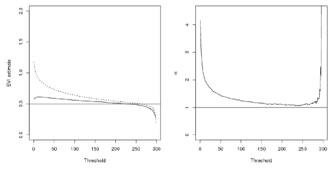
Figure 1: Left side: EVI estimates of the SP (dashed line) and TLPa (solid line). Right side: $\alpha$ estimate to TLPa.

Case 2

300 observations are simulated from a Fréchet distribution with $\gamma=1.33$ and $\text{EVI}=\nicefrac{{1}}{{\gamma}}=0.75.$ The outcomes are similar to the outcomes from Figure 1. Figure 2 shows the EVI estimates (of the SP and TLPa) and the estimate of $\alpha$ in the TLPa model. $\alpha$ moves towards 1 around the $220^{\text{th}}$ to $260^{\text{th}}$ sorted observations. This corresponds to where the $EVI$ estimate (Figure 2 left) reaches the true EVI value of 0.75.

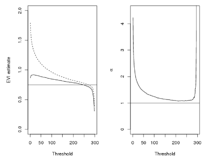
Figure 2: Left side: EVI estimates of the SP (dashed line) and TLPa (solid line). Right side: $\alpha$ estimate to TLPa.

Case 3

300 observations are simulated from the Burr Type XII distribution with $F\left(x\right)=1-\left(\frac{\eta}{\eta+x^{\tau}}\right)^{\lambda},\;x,\eta,\tau,\lambda>0$ with $EVI=\nicefrac{{1}}{{\lambda\tau}}$. Let $\lambda=1$, $\tau=1$ and $\eta=1$, therefore the $\text{EVI}=1$. The simulation process is again repeated 1000 times. Figure 3 shows the EVI estimates and the estimate of $\alpha$ in the TLPa model. The parameter estimates were obtained as the average over the 2000 posterior simulations as well as the average over the 1000 repetitions. Figure 3 shows that $\alpha$ moves towards 1 as the threshold increases and is the closest to 1 for threshold values from the $240^{\text{th}}$ to the $280^{\text{th}}$ sorted observation. This corresponds with the threshold values where the EVI estimate reaches the true $EVI$ estimate of 1.

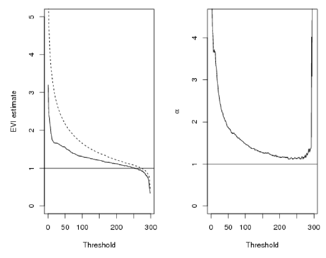
Figure 3: Left side: EVI estimates of the SP (dashed line) and TLPa (solid line). Right side: $\alpha$ estimate to TLPa.

It can be seen from the above cases that the EVI estimates of the TLPa is more stable, and less sensitive to the threshold choice, than the EVI estimate of the SP. This is expected since the variance of $\gamma_{\text{TLPa}}\left|\alpha,\boldsymbol{y}\right.,$ decreases as the value of $\alpha$ increases, see (12) and (16).

5 Real data example

In this section the wave height data from Newlyn, Cornwall, is considered as a real data example. A POT approach is used to model this data set and according the the mean residual plot a marginal threshold is chosen at 6.1 meters, see Coles (2001). The data observations with $n=2894$ is given in Figure 4. Extreme observations can easily be observed from the figure. Figure 5 shows the EVI estimates of the two models (left) and the estimate of $\alpha$ (right) for the TLPa model. Figure 5 shows that $\alpha$ moves towards 1 around the $2800^{\text{th}}$ sorted observation. This corresponds to a wave height of 6.67 meters which is close to the 6.1 meters threshold chosen by Coles (2001). The data set can be obtained from the ismev package in R.

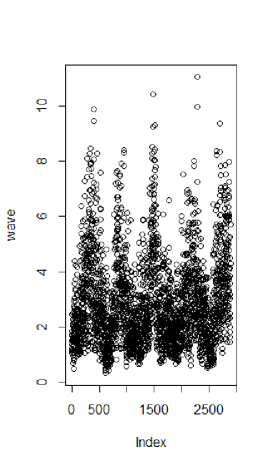
Figure 4: Wave height data observations.

The threshold was chosen as the $2800^{\text{th}}$ sorted observation and the quantiles (above the chosen threshold) for these two models were calculated by assuming the estimated parameter values at this threshold. As shown in Figure 6 the log quantile-quantile plot of both distributions indicates a good fit. This is expected since the threshold of 2800 seems to be optimal from Figure 5.

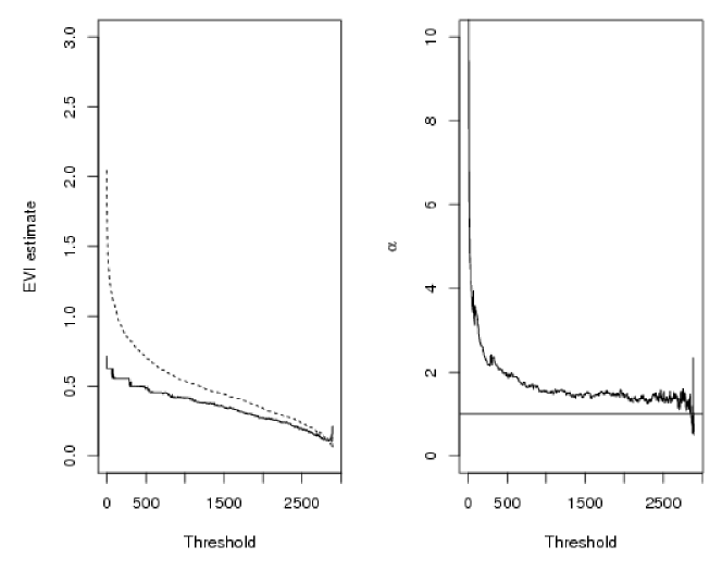
Figure 5: EVI estimates (top) and the estimate of $\alpha$ (bottom) in the TLPa model.

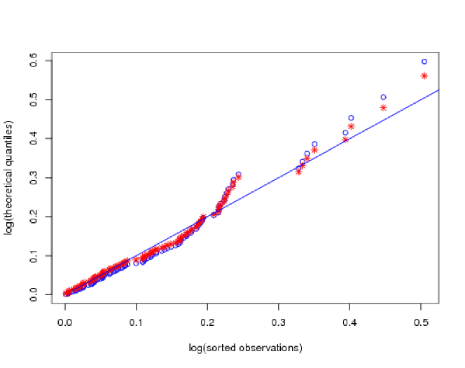
Figure 6: The log of the SP quantiles (in blue $\circ$) and the log of the TLPa quantiles (in red $*$) against the log of the sorted observations.

6 Procedure to choose a threshold

Since the main focus of this paper is on threshold choice and not bias reduction this section introduces a practical and modest method to choose a threshold. The conditional posterior of $\alpha$ from (15) is used. The advantage of this method is that the threshold can be chosen without visually inspecting a graph. Since $E\left(\alpha\left|\gamma,\boldsymbol{\bm{y}}\right.\right)=n\left(-\sum_{i=1}^{n}\text{log}\left(1-y_{i}^{-2\gamma}\right)\right)^{-1}$ and using the theory that as $n\rightarrow\infty$, $\alpha\rightarrow 1$, the method proposes to find the combination of $\gamma^{\#}$ and $u^{\#}$ (from a large spectrum of $\gamma$ and $u$ values) for which the Bayes estimate under squared error loss, $\left[E\left(\alpha\left|\gamma,\boldsymbol{\bm{y}}\right.\right)-1\right]^{2}$, is a minimum. Considering the above method two data sets are simulated for illustration purposes

i. $n=300$ observations from Fréchet $\left(\gamma=2\right)$.

ii. $n=300$ observations from Burr XII $\left(\lambda=1,\tau=1,\eta=1\right)$.

For data set (i) the $\text{EVI}_{\text{TLPa}}=\nicefrac{{1}}{{\left(2\gamma^{\#}\right)}}$ is chosen as 0.5383 and $u^{\#}$ is chosen as the $174^{\text{th}}$ sorted observation. For data set (ii) the $\text{EVI}_{\text{TLPa}}=\nicefrac{{1}}{{\left(2\gamma^{\#}\right)}}$ is chosen as 1.1230 and $u^{\#}$ is chosen as the $196^{\text{th}}$ sorted observation. For the real data example the $\text{EVI}_{\text{TLPa}}=\nicefrac{{1}}{{\left(2\gamma^{\#}\right)}}$ is chosen as 0.1158 and $u^{\#}$ is chosen as the $2850^{\text{th}}$ sorted observation ($u=7.52$). These chosen thresholds, together with the EVI estimates seem to be in line with the results obtained from the simulation studies (Figures 1 and 3) and the wave height application (Figure 5). The histogram with the chosen threshold (for the wave height date) is shown in Figure 7.

Figure 7: Histogram with the chosen threshold for the wave height data.

Another two data sets are simulated to test the appropriateness of the above method.

iii. $n_{1}=500$ observations from $\text{Normal}(\mu=5,\sigma^{2}=1)$ and $n_{2}=100$ observations from SP$(\gamma=5)$ and $u$ is chosen as the maximum Normal observation. The two simulated data sets are joined together as a single data set. The SP threshold is thus the $500^{\text{th}}$ sorted observation.

iv. $n_{1}=500$ observations from $\text{Normal}(\mu=10,\sigma^{2}=16)$ and $n_{2}=100$ observations from SP$(\gamma=2)$ and $u$ is chosen again as the maximum Normal observation. The two simulated data sets are joined together as a single data set. Again the SP threshold is the $500^{\text{th}}$ sorted observation.

Figure 8 shows the histogram of data set (iii) where the threshold is indicated with a vertical line. From Figure 8 it seems quite easy to visually distinguish between the two distributions. The threshold method is applied to the simulated data set where the threshold was chosen from the 50 percentile onward. An EVI-threshold pair that minimizes the Bayes estimate under squared error loss is selected. The process is repeated 1000 times. Table 1 shows the mean of the 1000 chosen thresholds as well as the mean of the $\text{EVI}_{\text{TLPa}}$ estimates. The chosen threshold seems to be rather close to the actual threshold and the EVI estimate is close to the true EVI, $\nicefrac{{1}}{{\gamma}}=0.2$.

Figure 9 shows the histogram of data set (iv) where the threshold is indicated with a vertical line. From Figure 9 it is not visually possible to distinguish between the two distributions, giving the smooth transition from the Normal distribution to the SP distribution. Table 2 shows the mean of the 1000 chosen thresholds as well as the mean of the $\text{EVI}_{\text{TLPa}}$ estimates. Since the transition between the two distribution are rather smooth the chosen threshold is not as close to the actual threshold but still reasonable and the $\text{EVI}_{\text{TLPa}}$ estimate is still rather close to the true EVI, $\nicefrac{{1}}{{\gamma}}=0.5$.

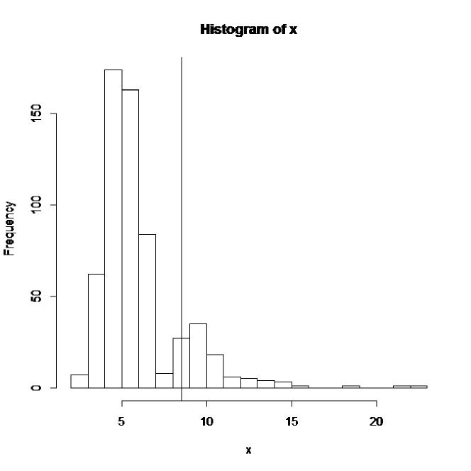
Figure 8: Histogram of data set (iii) with the chosen threshold indicated with the vertical line.

Table 1: Threshold estimate and $\text{EVI}_{\text{TLPa}}$ estimate.

Threshold estimate	$EVI$ estimate
457.339	0.2337

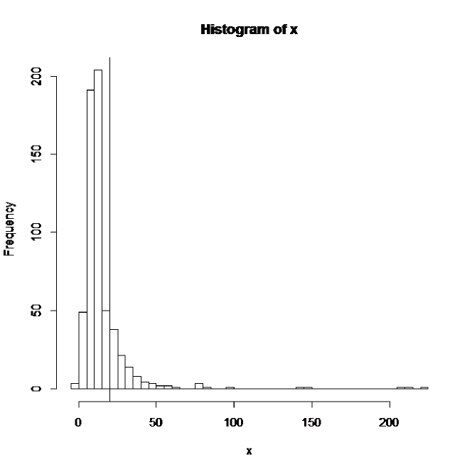
Figure 9: Histogram of data set (iv) with the chosen threshold indicated with the vertical line.

Table 2: Threshold estimate and $\text{EVI}_{\text{TLPa}}$ estimate.

Threshold estimate	$EVI$ estimate
442.786	0.4980865

7 Conclusion

In this study we have shown that the TLPa is a suitable model to use when modelling extreme events above a threshold when $\gamma>0$. The TLPa has proven to be less sensitive to the correct threshold choice. The focus of the study was to show that the $\alpha$ parameter of the TLPa can successfully contribute to choosing an appropriate threshold without using any visual technique.

A Bayesian approach was considered and the conditional posterior distributions of the two parameters of the TLPa was derived. These posteriors were valuable in the simulation studies. A method for choosing an optimum threshold was introduced. This method involves finding a combination of $\text{EVI}_{\text{TLPa}}$ and $u$ (threshold) values that minimizes the Bayes estimate under squared error loss. The illustrations in Section 6 shows that the method is easy to use with sufficient results.

References

• Beirlant, J., Dierckx, G., Goegebeur, Y., & Matthys, G. (1999). Tail index estimation and an exponential regression model. Extremes, 2(2), 177-200.

• Beirlant, J., Goegebeur, Y., Segers, J., & Teugels, J. (2004). Statistics of Extremes: Theory and Applications. Chichester: John Wiley and Sons.

• Beirlant, J., Joossens, E., & Segers, J. (2009). Second-order refined peaks-over-threshold modelling for heavy-tailed distribution. Journal of Statistical Planning and Inference, 139, 2800-2815.

• Beirlant, J., Maribe, G., & Verster, A. (2019). Using shrinkage estimators to reduce bias and mse in estimation of heavy tails. REVSTAT-Statistical Journal, 17(1), 91-108.

• Caeiro, F. & Gomes, M. I. (2011). Asymptotic comparison at optimal levels of reduced-bias extreme value index estimators. Statistica Neerlandica, 65(4), 462-488.

• Coles, S. G. (2001). An introduction to statistical modeling of extreme values. London: Springer.

• de Haan, L. & Ferreira, A. (2005). Extreme Value Theory: An Introduction. New York: Springer

• Feuerverger, A. & Hall, P. (1999). Estimating a tail exponent by modelling departure from a Pareto distribution. The Annals of Statistics, 27(2), 760-781.

• Gomes, M. I., Martins, M. J., & Neves, M. (2000). Alternatives to a semiparametric estimator of parameters of rare events - the jackknife methodology. Extremes, 3(3), 207-229.

• Rezaei, S., Sadr, B. B., Alizadeh, M., & Nadarajah, S. (2017). Topp-Leone generated family of distributions: Properties and applications. Communications in Statistics - Theory and Methods, 46(6), 2893-2909.

• Topp, C. W. & Leone, F. C. (1955). A family of J-shaped frequency functions. Journal of the American Statistical Association, 50, 209-219.

Appendix

Approximating the conditional posterior distribution of $\gamma$ given $\alpha$ and $\boldsymbol{y}$.

From the joint posterior in (14) the conditional posterior is

$$p\left(\gamma\left|\alpha,\boldsymbol{y}\right.\right) \propto\gamma^{n-1}e^{-2\gamma\sum_{i=1}^{n}\text{log}\left(y_{i}\right)}e^{\left(\alpha-1\right)\sum_{i=1}^{n}\text{log}\left(1-y_{i}^{-2\gamma}\right)}.$$

By using the Taylor series expansion, $e^{\left(\alpha-1\right)\sum_{i=1}^{n}\text{log}\left(1-y_{i}^{-2\gamma}\right)}$ can be approximated as $\prod_{i=1}^{n}\left(2\gamma\text{log}y_{i}\right)^{\alpha-1}$.

Therefore

$$p\left(\gamma\left|\alpha,\boldsymbol{y}\right.\right) \propto\gamma^{n-1}e^{-2\gamma\sum_{i=1}^{n}\text{log}\left(y_{i}\right)}\prod_{i=1}^{n}\left(2\gamma\text{log}y_{i}\right)^{\alpha-1}$$

$$\propto\gamma^{n\alpha-1}e^{-2\gamma\sum_{i=1}^{n}\text{log}\left(y_{i}\right)}.$$