Bayesian Experience Reuse for Learning from Multiple Demonstrators

Abstract

Learning from demonstrations (LfD) improves the exploration efficiency of a learning agent by incorporating demonstrations from experts. However, demonstration data can often come from multiple experts with conflicting goals, making it difficult to incorporate safely and effectively in online settings. We address this problem in the static and dynamic optimization settings by modelling the uncertainty in source and target task functions using normal-inverse-gamma priors, whose corresponding posteriors are, respectively, learned from demonstrations and target data using Bayesian neural networks with shared features. We use this learned belief to derive a quadratic programming problem whose solution yields a probability distribution over the expert models. Finally, we propose Bayesian Experience Reuse (BERS) to sample demonstrations in accordance with this distribution and reuse them directly in new tasks. We demonstrate the effectiveness of this approach for static optimization of smooth functions, and transfer learning in a high-dimensional supply chain problem with cost uncertainty.

1 Introduction

Learning from demonstrations (LfD) is a powerful approach to incorporate advice from experts in the form of demonstrations in order to speed up learning on new tasks. However, existing work in LfD assumes that demonstrations are generated from a single near-optimal agent with a single goal [3, 14, 38]. In practice, however, data may be available from multiple sub-optimal agents with conflicting goals. For example, when learning to operate a vehicle autonomously using human driver demonstrations [9], different drivers can have different goals and needs (e.g. destinations, priorities for safety or time) and experience levels. Relying on demonstrators whose goals are misaligned with the new target task can lead to unintended behaviors, which can be dangerous in performance-critical applications, and can be minimized by learning to trust the most relevant demonstrators.

In this paper, we focus on using LfD with multiple conflicting demonstrators for solving static and dynamic optimization problems. In order to measure the similarity between source and target task goals, we adopt a Bayesian framework. We first parameterize source and target task reward functions as linear functions in a common feature space, whose uncertainty is modeled using Normal-Inverse-Gamma priors that are updated to posterior distributions using source and target demonstrations. Taking a fully Bayesian treatment allows us to avoid premature convergence and is more robust to non-stationary data [8]. To jointly learn the posteriors and feature space, we build a Bayesian neural network with a shared encoder and multiple heads, one for each source and target task. We then formulate a quadratic programming problem (QP) whose solution yields a probability distribution over the source demonstrators. This allows us to trade-off the mean and variance of the uncertainty in source and target task goals in a principled manner.

In order to transfer demonstrations to new tasks in LfD, one approach is to pre-train the learner directly from the source data [15], or learn and reuse auxiliary representations from the source data such as policies [16, 45]. However, the former can be ineffective when demonstrations assume conflicting goals, while meaningful policies may be difficult to solicit from the latter when demonstrators are limited, sub-optimal or exploratory in nature [32, 38, 47]. On the other hand, experience collected from a failed or inexperienced demonstrator can be just as valuable as an experienced one [21]. We present an algorithm called Bayesian Experience Reuse (BERS), for directly reusing multiple demonstrations in a way that is consistent with the learned weighting over the source and target task goals (Algorithm 1). We demonstrate the efficacy of our approach for optimizing static functions, and continuous control of a supply chain using reinforcement learning with high-dimensional actions.

1.1 Related Work

Most papers in LfD incorporate demonstrations from a single optimal or near-optimal expert with a single goal [3, 14, 38]. Some papers in the area of LfD for reinforcement learning (RLfD) relax this assumption to a single sub-optimal demonstrator, using pre-training [15, 19, 22], reward shaping [13, 42], ranking demonstrations [51], Bayesian inference [36], or other approaches [45] for transfer. However, the aforementioned papers cannot learn from multiple demonstrators with conflicting goals. On the other hand, papers on this topic typically assume multiple near-optimal demonstrators, so that recovering policies [16, 28, 29], value functions [20, 27] or successor features [6, 7] is possible. In this paper, we show how sub-optimal demonstrators with conflicting goals can be ranked according to their alignment with the target task goal in a safe Bayesian manner, and reused directly by the target agent without learning auxiliary representations such as policies or value functions. Our approach is related to encoder sharing [18, 34, 48, 49] and uncertainty quantification of rewards or policies [5, 12, 25, 46], but our problem setting and methodology are different.

2 Background

2.1 Reinforcement Learning

Complex decision-making can be summarized in a Markov decision process (MDP), formally defined as a five-tuple $\langle\mathcal{S},\mathcal{A},P,R,\gamma\rangle$, where: $\mathcal{S}$ is a set of states, $\mathcal{A}(s)$ is a set of possible actions in state $s$, $P(\cdot|s,a)$ gives the next-state distribution upon taking action $a$ in state $s$, $R(s,a,s^{\prime})$ is the reward received upon transition to state $s^{\prime}$ after taking action $a$ in state $s$, and $\gamma\in[0,1]$ is a discount factor that gives smaller priority to rewards realized further into the future. The objective of an agent is to find a policy $\mu:\mathcal{S}\to\mathcal{A}$ that maximizes the long-run expected return $Q^{\mu}(s,a)=\mathbb{E}[\sum_{t=0}^{\infty}\gamma^{t}R(s_{t},a_{t},s_{t+1})\,|\,s_{0}=s,a_{0}=a]$, where $a_{t}\sim\mu(s_{t})$ and $s_{t+1}\sim P(\cdot|s_{t},a_{t})$.

When $P$ and $R$ are known, an optimal policy can be found exactly using dynamic programming [35, 37]. In the reinforcement learning setting, neither $P$ nor $R$ are known to the decision-maker. Instead, the agent interacts with the environment using a randomized exploration policy $\mu^{e}$, collecting reward and observing the state transitions [43]. In order to learn optimal policies in this setting, temporal difference methods first learn $Q(s,a)$ and then recover an optimal policy [31, 52], while policy gradient methods parameterize and recover an optimal policy $\mu^{*}$ directly [44]. Actor-critic methods learn and use both a critic $Q(s,a)$ and actor policy $\mu(s)$ simultaneously [26].

2.2 Common Feature Representations

In this paper, we consider the regression problem associated with learning a multivariate function $y:\mathcal{X}\to\mathbb{R}$ on a domain $\mathcal{X}$. For instance, in the RL setting, we estimate reward functions where $\mathcal{X}=\mathcal{S}\times\mathcal{A}\times\mathcal{S}$ and $y(\mathbf{x})=R(s,a,s^{\prime})$. Given a feature map $\bm{\phi}:\mathcal{X}\to\mathbb{R}^{d}$, a function $y$ can be expressed as a linear combination $y(\mathbf{x})=\bm{\phi}(\mathbf{x})^{\top}\mathbf{w},\,\forall x\in\mathcal{X}$, where $\mathbf{w}\in\mathbb{R}^{d}$ is a fixed vector.

We are interested in the transfer learning problem between similar tasks in a domain $\mathcal{M}^{\bm{\phi}}$ on a common $\mathcal{X}$, defined formally as

$$\mathcal{M}^{\bm{\phi}}=\left\{y\,:\,\exists\mathbf{w}\in\mathbb{R}^{d}\textit{ s.t. }y(\mathbf{x})=\bm{\phi}(\mathbf{x})^{\top}\mathbf{w},\,\forall\mathbf{x}\in\mathcal{X}\right\}.$$ (1)

In the RL setting, $\mathcal{M}^{\bm{\phi}}$ could include all MDPs with shared dynamics and different rewards $R_{i}$. In (1), we have explicitly assumed that the (unknown) state features $\bm{\phi}$ are shared among tasks. This is not a restrictive assumption in practice, as given a set of tasks $T_{1},T_{2}\dots T_{n}\in\mathcal{M}^{\bm{\phi}}$, we may trivially define $\phi_{k}(\mathbf{x})=y_{T_{k}}(\mathbf{x}),\,\forall\mathbf{x}\in\mathcal{X}$ for each $k=1,2\dots n$. The main challenge in this paper is to simultaneously learn a suitable common latent feature embedding $\bm{\phi}$ and posterior distributions for $y(\mathbf{x})$, and leverage this uncertainty for measuring task similarity in $\mathcal{M}^{\bm{\phi}}$.

3 Bayesian Learning from Multiple Demonstrators

The agent is presented with sets of demonstrations $\mathcal{D}_{1},\mathcal{D}_{2},\dots\mathcal{D}_{N}$ from source tasks $T_{1},T_{2},\dots T_{N}\in\mathcal{M}^{\bm{\phi}}$, consisting of labeled pairs $(\mathbf{x}_{t},y_{t})$, and would like to solve a new target task $T_{target}\in\mathcal{M}^{\bm{\phi}}$. In order to make optimal use of the source tasks during training, the agent should learn to favor demonstrators whose underlying reward representation is closest to the target reward.

3.1 Bayesian Linear Regression with Common Feature Representations

In order to tractably learn these reward representations, we learn a shared feature space $\hat{\bm{\phi}}\approx\bm{\phi}$, together with Bayesian regressors $\mathbb{P}(\mathbf{w}_{i}|\mathcal{D}_{i})$ for the source task and a Bayesian regressor $\mathbb{P}(\mathbf{w}_{target}|\mathcal{D})$ for the target task such that $y_{i}(\mathbf{x})=\bm{\phi}(\mathbf{x})^{\top}\mathbf{w}_{i}$ and $y_{target}(\mathbf{x})=\bm{\phi}(\mathbf{x})^{\top}\mathbf{w}_{target}$ approximately hold for all $i$ and all realizations $\mathbf{x}\in\mathcal{X},\,y\in\mathbb{R}$. As we will soon show, the sharing of the features $\bm{\phi}$ is crucial to allow meaningful comparisons between source weights $\mathbf{w}_{i}$ and target weights $\mathbf{w}$.

In order to tractably learn the features $\bm{\phi}$ as well as the corresponding posterior distributions, we parameterize $\bm{\phi}(\mathbf{x})\approx\bm{\phi}_{\bm{\theta}}(\mathbf{x})$ using a deep neural network (encoder) with weight parameters $\bm{\theta}$, and model $\mathbf{w}_{1},\dots\mathbf{w}_{N},\mathbf{w}_{target}$ using the normal-inverse-gamma (NIG) conjugate prior:

$$y_{i}(\mathbf{x})=\bm{\phi}_{\bm{\theta}}(\mathbf{x})^{\top}\mathbf{w}_{i}+\varepsilon_{i},$$ (2)

$$\varepsilon_{i}\sim\mathcal{N}(0,\sigma_{i}^{2}),\quad\quad\mathbf{w}_{i}\sim\mathcal{N}(\bm{\mu}_{i},\sigma_{i}^{2}\bm{\Lambda}_{i}^{-1}),\quad\quad\sigma_{i}^{2} \sim\mathrm{InvGamma}(\alpha_{i},\beta_{i}).$$

The joint posterior $\mathbb{P}(\mathbf{w}_{i},\sigma_{i}^{2}|\mathcal{D}_{i})$ can be shown to factor as

$$\mathbb{P}(\mathbf{w}_{i},\sigma_{i}^{2}|\mathcal{D}_{i})\propto\mathbb{P}(\mathbf{w}_{i}|\sigma_{i}^{2},\mathcal{D}_{i})\,\mathbb{P}(\sigma_{i}^{2}|\mathcal{D}_{i}),$$ (3)

where $\mathbf{w}_{i}|\sigma_{i}^{2},\mathcal{D}_{i}\sim\mathcal{N}(\bm{\mu}_{i},\sigma_{i}^{2}\bm{\Lambda}_{i}^{-1})$ and $\sigma_{i}^{2}|\mathcal{D}_{i}\sim\mathrm{InvGamma}(\alpha_{i},\beta_{i})$, where:

$$\bm{\Lambda}_{i}=\bm{\Lambda}_{i}^{0}+\bm{\Phi}_{i}^{\top}\bm{\Phi}_{i}, \quad\quad\bm{\mu}_{i}=\bm{\Lambda}_{i}^{-1}\left(\bm{\Lambda}_{i}^{0}\bm{\mu}_{i}^{0}+\bm{\Phi}_{i}^{\top}\mathbf{y}_{i}\right),$$ (4)

$$\alpha_{i}=\alpha_{i}^{0}+\frac{1}{2}|\mathcal{D}_{i}|, \quad\quad\beta_{i}=\beta_{i}^{0}+\frac{1}{2}\left(\mathbf{y}_{i}^{\top}\mathbf{y}_{i}+(\bm{\mu}_{i}^{0})^{\top}\bm{\Lambda}_{i}^{0}\bm{\mu}_{i}^{0}-\bm{\mu}_{i}^{\top}\bm{\Lambda}_{i}\bm{\mu}_{i}\right),$$

and where $\bm{\Phi}_{i}$ is the set of state features and $\mathbf{y}_{i}$ is the set of observations of $y_{i}$ in $\mathcal{D}_{i}$ [8]. We have also assumed that, conditional on data $\mathcal{D}_{i}$, weights $\mathbf{w}_{i}$ and variances $\sigma_{i}^{2}$ are mutually independent between tasks, a very mild assumption in practice. Adapting the methodology of Snoek et al. [40], we update $\bm{\theta}$ by gradient ascent on the marginal log-likelihood function for each head $i$, defined here as

$$\log\mathbb{P}(\mathbf{y}_{i}|\mathbf{X}_{i})=|\mathcal{D}_{i}|\pi+\log\Gamma(\alpha_{i}^{0})-a_{i}^{0}\log\beta_{i}^{0}+\frac{1}{2}\log|\bm{\Lambda}_{i}^{0}|-\log\Gamma(\alpha_{i})+\alpha_{i}\log\beta_{i}-\frac{1}{2}\log|\bm{\Lambda}_{i}|,$$ (5)

where the key quantities are provided by (4) and depend implicitly on $\bm{\theta}$ through $\bm{\Phi}_{i}$.

Using this model, parameter sharing allows the learned features $\bm{\phi}$ to be refined and transferred seamlessly from source to target tasks, or as new source and target tasks are incorporated, and provides an additional source of knowledge for transfer. However, our main contribution is to use the posterior distributions over task goals, $\mathbf{w}_{i}$ and $\mathbf{w}_{target}$, to transfer experiences between tasks.

3.2 Source Task Selection via Quadratic Programming

In order to derive a Bayesian decision rule for source task selection, we first observe that source tasks that are most similar to the target task, and hence those that lead to better transfer, should have $\mathbf{w}_{i}$ closest to the true target $\mathbf{w}_{target}$. In our setting, we instead have uncertain estimates for $\mathbf{w}_{i}$ and $\mathbf{w}_{target}$ modelled as multivariate normal random variables. We therefore look for a weighting $\sum_{i=1}^{N}a_{i}\mathbf{w}_{i}$ that is closest in expectation to $\mathbf{w}_{target}$ with respect to the uncertainty in these estimates.

More specifically, suppose that we have computed the posterior distributions of $\mathbf{w}_{i}$ for each $i=1,2\dots N$ and $\mathbf{w}_{target}$ from past data. We would like to weight the $\mathbf{w}_{i}$ in such a way that the weighted sum $\sum_{i}a_{i}\mathbf{w}_{i}$ is closest to $\mathbf{w}_{target}$ in expectation, or in other words, solve

$$\min_{\mathbf{a}\in\mathcal{P}}\mathbb{E}\left[\|\mathbf{w}_{target}-\sum_{i=1}^{N}a_{i}\mathbf{w}_{i}\|_{2}^{2}\,\Big{|}\,\mathcal{D}\right],$$ (6)

where $\mathcal{D}$ is the union of all source and target data and $\mathcal{P}$ is a convex polyhedron. Specifically, we would like to be able to sample source tasks according to $\mathbf{a}$, so we take $\mathcal{P}=\{\mathbf{a}:\mathbf{1}^{\top}\mathbf{a}=1,\,\mathbf{a}\geq\mathbf{0}\}$, the set of probability distributions on $\{1,2\dots N\}$. In other applications, such as static regression problems [33, 50, 53], we may choose $\mathcal{P}=\mathbb{R}^{N}$ or put additional constraints on expert selection.

To derive a closed form for (6), first note that, given the true values of the variances $\mathbf{v}=[\sigma_{1}^{2},\dots\sigma_{N}^{2},\sigma_{target}^{2}]$, the random variables $\mathbf{w}_{1},\dots\mathbf{w}_{N},\mathbf{w}_{target}$ follow normal distributions with respective means $\bm{\mu}_{1}\dots\bm{\mu}_{N},\bm{\mu}_{target}$ and covariances $\sigma_{1}^{2}\bm{\Sigma}_{1},\dots\sigma_{N}^{2}\bm{\Sigma}_{N},\sigma_{target}^{2}\bm{\Sigma}_{target}$ (equation (3)). Then, for any $\mathbf{a}\in\mathbb{R}^{N}$, it is easy to check that $\mathbf{w}_{target}-\sum_{i}a_{i}\mathbf{w}_{i}\,|\,\mathbf{v},\mathcal{D}\sim\mathcal{N}(\bm{\mu}_{target}-\sum_{i}a_{i}\bm{\mu}_{i},\sigma_{target}^{2}\bm{\Sigma}_{target}+\sum_{i}a_{i}^{2}\sigma_{i}^{2}\bm{\Sigma}_{i})$, and hence that

$$\mathbb{E}\Big{[}\|\mathbf{w}_{target}-\sum_{i}a_{i}\mathbf{w}_{i}\|_{2}^{2}\,|\,\mathbf{v},\mathcal{D}\Big{]} =\mathrm{tr}(\sigma_{target}^{2}\bm{\Sigma}_{target}+\sum_{i}a_{i}^{2}\sigma_{i}^{2}\bm{\Sigma}_{i})+\|\bm{\mu}_{target}-\sum_{i}a_{i}\bm{\mu}_{i}\|_{2}^{2}$$

$$=\sigma_{target}^{2}\mathrm{tr}(\bm{\Sigma}_{target})+\sum_{i}a_{i}^{2}\sigma_{i}^{2}\mathrm{tr}(\bm{\Sigma}_{i})+\|\bm{\mu}_{target}-\sum_{i}a_{i}\bm{\mu}_{i}\|_{2}^{2}.$$ (7)

Then, taking expectation of (7) with respect to the variance terms $\mathbf{v}$,

$$\mathbb{E}\Big{[}\|\mathbf{w}_{target}-\sum_{i}a_{i}\mathbf{w}_{i}\|_{2}^{2}\,\big{|}\,\mathcal{D}\Big{]} =\mathbb{E}\left[\mathbb{E}\Big{[}\|\mathbf{w}_{target}-\sum_{i}a_{i}\mathbf{w}_{i}\|_{2}^{2}\,\big{|}\,\mathbf{v},\mathcal{D}\Big{]}\,\Big{|}\,\mathcal{D}\right]$$

$$\propto\sum_{i}a_{i}^{2}\,\mathbb{E}[\sigma_{i}^{2}|\mathcal{D}]\,\mathrm{tr}(\bm{\Sigma}_{i})+\|\bm{\mu}_{target}-\sum_{i}a_{i}\bm{\mu}_{i}\|_{2}^{2}$$

$$=\sum_{i=1}^{N}a_{i}^{2}\left(\frac{\beta_{i}}{\alpha_{i}-1}\right)\mathrm{tr}(\bm{\Sigma}_{i})+\|\bm{\mu}_{target}-\sum_{i=1}^{N}a_{i}\bm{\mu}_{i}\|_{2}^{2},$$ (8)

where in the last step we used (2) and the expectation of $\mathrm{InvGamma}(\alpha_{i},\beta_{i})$, and ignored all terms independent of any decision variables $\mathbf{a}$. Hence, we have shown that optimizing the expected weighted mean-squared error (6) is equivalent to optimizing the weighted mean-squared error of the posterior means plus a penalty term equal to the product of the noise and posterior variances.

To simplify (8) further, we define $\mathbf{M}=[\bm{\mu}_{1}\,\dots\bm{\mu}_{N}]\in\mathbb{R}^{d\times N}$ and $\mathbf{S}\in\mathbb{R}^{N\times N}$ the diagonal matrix with entries $\frac{\beta_{i}}{\alpha_{i}-1}\mathrm{tr}(\bm{\Sigma}_{i}),\,i=1,2\dots N$. Rewriting (8) in this new notation, we can obtain the following quadratic programming formulation of our problem:

$$\!\min_{\mathbf{a}} -\bm{\mu}^{\top}\mathbf{M}\mathbf{a}+\frac{1}{2}\mathbf{a}^{\top}(\mathbf{M}^{\top}\mathbf{M}+\mathbf{S})\mathbf{a}$$ (9)

subject to $$\mathbf{1}^{\top}\mathbf{a}=1,$$

$$\mathbf{a}\succeq\mathbf{0}.$$

Here, $\mathbf{M}^{\top}\mathbf{M}+\mathbf{S}$ is positive definite, since it is the sum of the positive semi-definite $\mathbf{M}^{\top}\mathbf{M}$ and the positive definite $\mathbf{S}$. Hence, the above QP problem can be formulated and solved exactly using an off-the-shelf solver in polynomial time in $N$ [11], which does not grow with the feature dimension $d$ nor the number of demonstrations $|\mathcal{D}_{i}|$ and can be applied in online settings. Hence, the QP (9) remains tractable when the domain complexity is high or the number of demonstrations is large. This is not necessarily the case if omitting the second order terms $\mathbf{S}$, since the QP may become rank-deficient and thus lack a unique solution. We can therefore interpret $\mathbf{S}$ as a data-dependent Bayesian regularizer for the QP solution.

In the case where $N$ is considerably large, the solution to (9) can instead be approximated using neural networks [1, 10]. Alternatively, since the posterior updates are relatively smooth (as we demonstrate experimentally), the solution of (9) should not change significantly between consecutive iterations, in which case warm starts may be particularly effective [17].

3.3 Bayesian Experience Reuse (BERS) for LfD

When transferring demonstrations from a single source, a simple yet effective approach is to pre-train or seed the target learning agent with the demonstrations prior to target task training [15]. When data originates from multiple demonstrators with differing goals, pre-training is no longer possible. Instead, we propose to train the target agent on the source data while concurrently learning the target task. In this manner, the source demonstrations provide an effective exploration bonus by allowing the agent to observe demonstrations from other tasks with similar goals.

More specifically, in each iteration of the target learning phase, we sample a source task $T_{i}\in\mathcal{M}^{\bm{\phi}}$ according to the probability distribution $\mathbf{a}$ obtained from the quadratic programming problem (9), and train the target agent on experiences drawn from the corresponding source data $\mathcal{D}_{i}$. In order for the target agent to improve beyond the source task solution and generalize to the new task, the agent must eventually learn from target demonstrations rather than the source data. In order to do this, we apply the framework of Probabilistic Policy Reuse [16, 29] in our setting. Specifically in each training episode $m$, the target agent is trained on source data with probability $p_{m}$, and otherwise uses target data with probability $1-p_{m}$, where $p_{m}$ is annealed to zero over time. The choice of $p_{m}$ is typically problem dependent, but may also be annealed based on the QP solution.

The full implementation of our algorithm, Bayesian Experience Reuse (BERS), is illustrated in Figure 1 in a transfer learning setting. The left figure provides a visualization of the process used to weight source tasks. Here, Bayesian heads with parameters $\{\bm{\mu}_{i},\bm{\Lambda}_{i},\alpha_{i},\beta_{i}\}_{i=1}^{N}$ and $\bm{\mu},\bm{\Lambda},\alpha,\beta$ are maintained for source and target tasks respectively, while sharing the encoder parameters $\bm{\theta}$, and then used to construct the quadratic programming problem (9). The outputs $\hat{y}_{i}$ and $\hat{y}_{target}$ can also be used for making predictions (e.g. in regression tasks); in this paper we focus on using the posterior distributions over task goals, and the corresponding QP solution, to transfer source demonstrations in a Bayesian framework.

In the pseudo-code on the right, we have defined $O_{base}$ to be a base learning algorithm for solving the target task, which is assumed to be a static or dynamic (RL) optimization algorithm in this work. We pre-train the first $N$ heads on source data to learn features and posteriors for source task goals. At the end of each episode, we train all source and target heads on source and target demonstrations to refine the features and posteriors for all tasks. With simple modifications, this algorithm can also be applied in multi-task settings, by maintaining one QP solution per task. The bottleneck of this procedure is the solution of the QP, which can be addressed using various approximation methods outlined above.

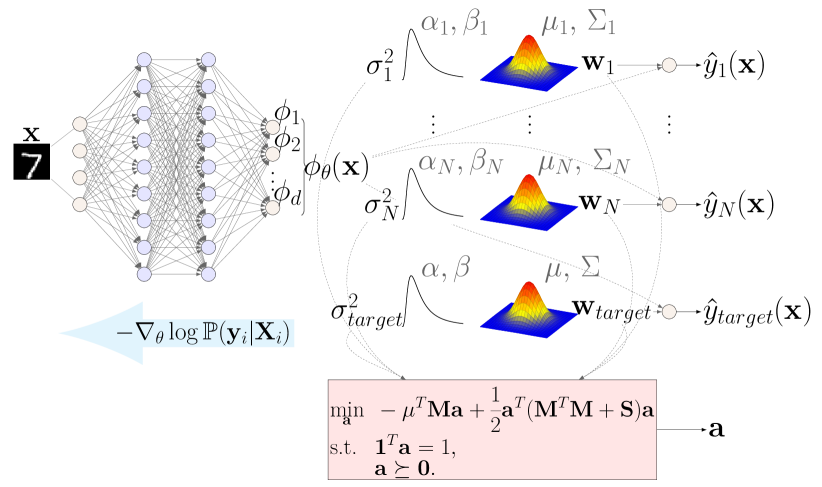
Algorithm 1 Bayesian Experience Reuse (BERS)

0: $\{\mathcal{D}_{i}\}_{i=1}^{N}$, $T_{N+1}=T_{target}\in\mathcal{M}^{\bm{\phi}}$, $O_{base}$, $\mathcal{D}_{N+1}=\mathcal{D}_{target}=\emptyset$, $\bm{\theta}$, $\{\bm{\mu}_{i},\bm{\Lambda}_{i},\alpha_{1},\beta_{i}\}_{i=1}^{N+1}$, $p_{m}$, $\mathbf{a}$

 pre-train $\bm{\theta}$, $\{\bm{\mu}_{i},\bm{\Lambda}_{i},\alpha_{1},\beta_{i}\}_{i=1}^{N}$ on $\{\mathcal{D}_{i}\}_{i=1}^{N}$ using (4), (5)

 for episode $m=1,2,\dots$ do

    for step $t=1,2,\dots T$ of episode $m$ do

       explore $T_{target}$ using $O_{base}$ and collect $d=(\mathbf{x},y)$

       $\mathcal{D}_{target}=\mathcal{D}_{target}\cup d$

       if $\mathrm{Bernoulli}(p_{m})=1$ then

          sample $i_{t}\sim\mathbf{a}$ and experience $\mathcal{B}\subset\mathcal{D}_{i_{t}}$

       else

          sample experience $\mathcal{B}\subset\mathcal{D}_{target}$

       end if

       train $O_{base}$ on $\mathcal{B}$

    end for

    train $\bm{\theta}$, $\{\bm{\mu}_{i},\bm{\Lambda}_{i},\alpha_{1},\beta_{i}\}_{i=1}^{N+1}$ on $\{\mathcal{D}_{i}\}_{i=1}^{N+1}$ using (4), (5)

    solve QP (9) (using, e.g. [2]) and set $\mathbf{a}$ to the solution

 end for

 return $O_{base}$

Figure 1: Left: bayesian multi-headed neural-linear model with shared encoder (MLP) and aggregated QP decision layer. Right: pseudo-code implementation for transfer learning for static and dynamic optimization (BERS).

4 Empirical Evaluation

In order to demonstrate the effectiveness of BERS, we apply it to a static optimization problem and continuous control of a supply chain.

4.1 Static Function Optimization

We first consider the problem of minimizing a smooth function [24]. Transfer learning can be useful in this setting because the known solution of one smooth function can be used as a starting point or seed in the search for the minimum of another similar function. More specifically, we use the 10-D Rosenbrock, Ackley and Sphere functions as source tasks, whose global optimum solutions have been shifted to various locations. As target task, we use each source task as the ground truth as well as the Rastrigin function. The Sphere and Rastrigin functions are locally similar around the optimum, so a successful transfer experiment should learn to transfer knowledge between them. We consider optimizing the Rastrigin function in both transfer and multi-task settings. As the base learning agent $O_{base}$ in Algorithm 1, we use Differential Evolution (DE) [41], a commonly-used evolutionary algorithm for global optimization of black-box functions .

We compare BERS (Ours) to the UCB algorithm [4] with asymptotically optimal convergence (UCB), where the reward is improvement in best solution value between consecutive iterations. We also compare to the equal weighting of demonstrators (Equal), individual demonstrators (S1, S2…), and standard DE (None). Figure 2 illustrates the function value of the best solution and the QP solution in each iteration. Figure 3 tracks the movement of the posterior means of $\mathbf{w}_{i}$ and $\mathbf{w}_{target}$ during target training for a simplified model with $d=2$ for visualization.

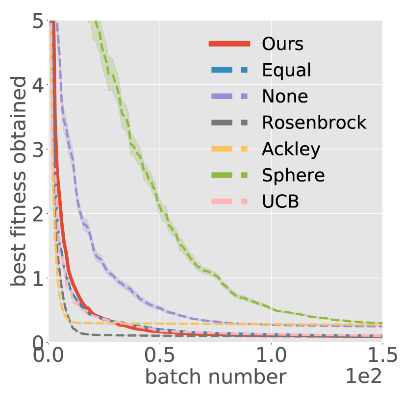
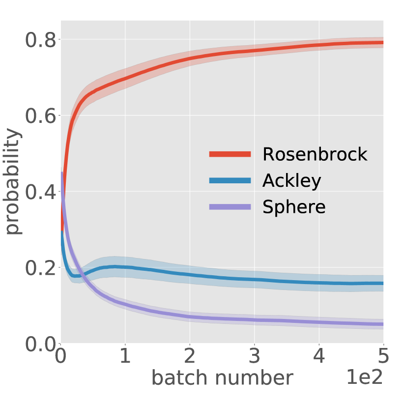
(a) Rosenbrock

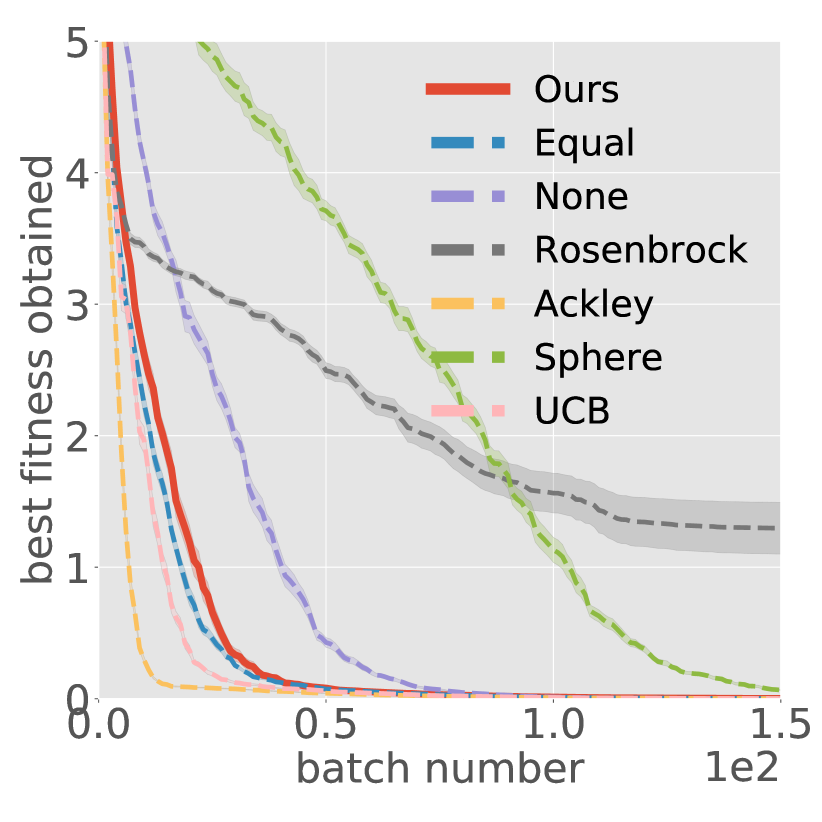
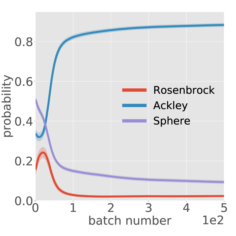
(b) Ackley

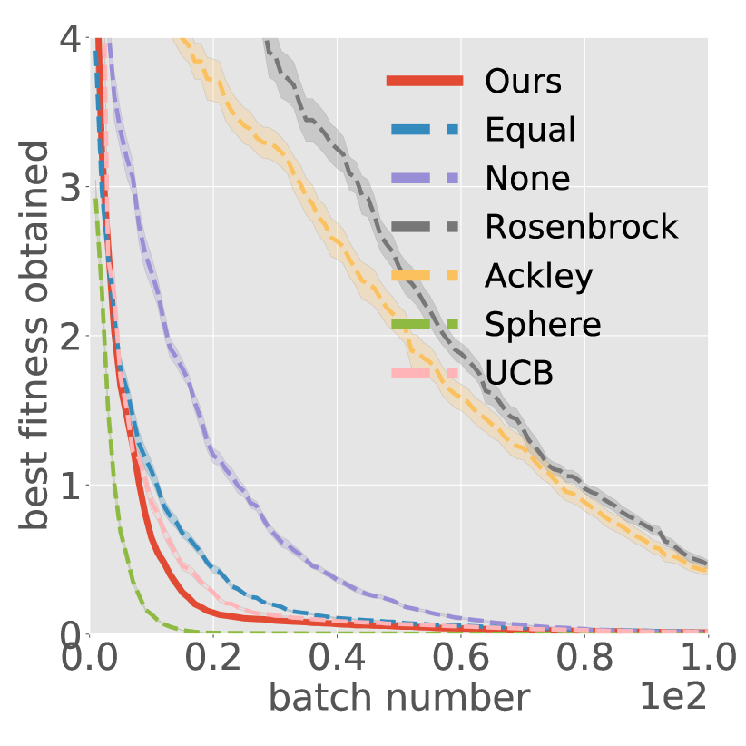
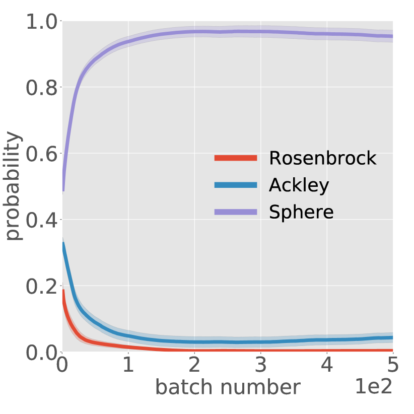
(c) Sphere

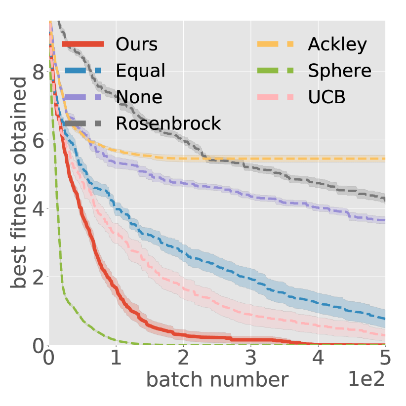
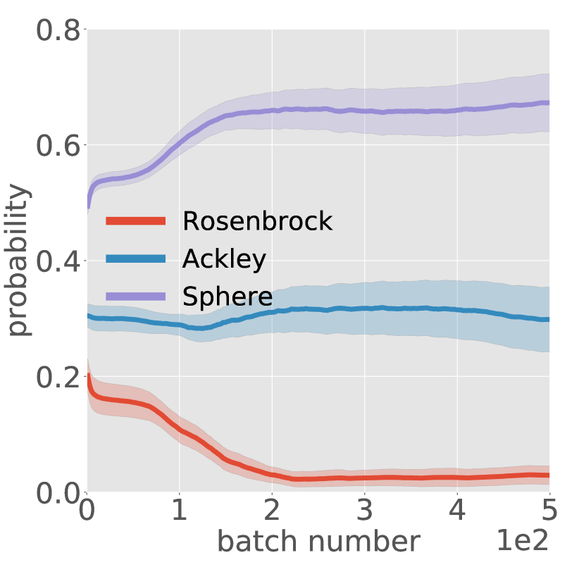
(d) Rastrigin

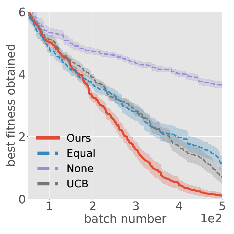
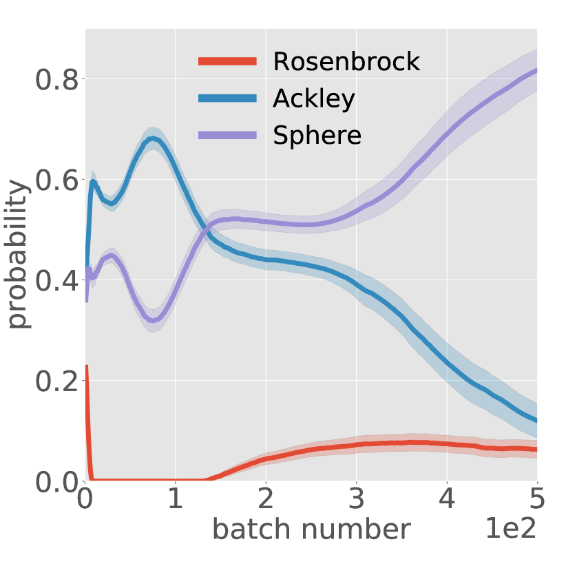
(e) Rastrigin-MT

Figure 2: Best function fitness (top row) and weights assigned to source tasks (bottom row) over generations using transfer and multi-task (MT) learning for function optimization, with each source and target task as ground truth. Averaged over 20 trials with shaded standard error bars.

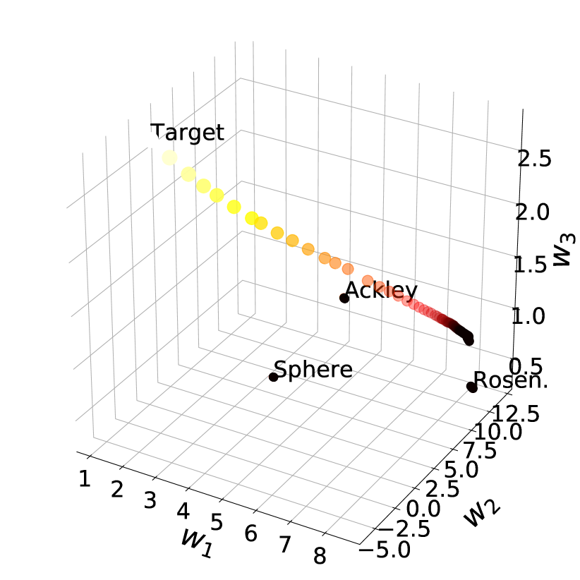
(a) Rosenbrock

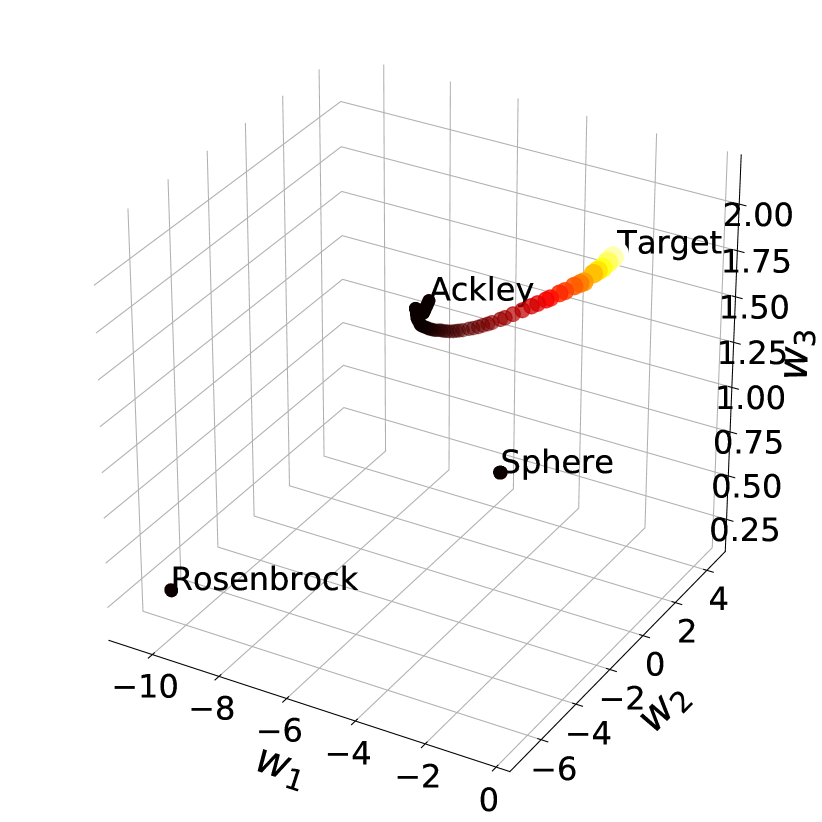
(b) Ackley

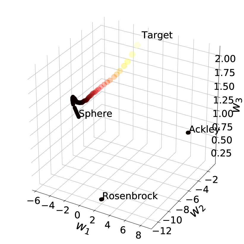
(c) Sphere

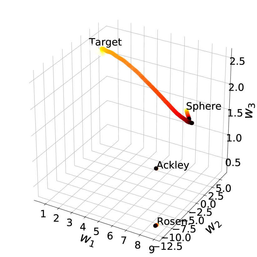
(d) Rastrigin

Figure 3: For function optimization with each source and target task as the ground truth, shows the evolution of the posterior mean of each $\mathbf{w}_{i}$ and $\mathbf{w}_{target}$ during training for the simplified experiment with latent dimension $d=2$. As shown here, the target mean eventually converges to the correct source task mean.

4.2 Continuous Control of a Supply Chain Network

The second problem is continuous control of a supply chain network as illustrated in Figure 4(a). Here, the nodes include a central factory and $K=6$ warehouses (denoted A, B …F), and edges represent possible transportation routes along which inventory can flow. A centralized controller must decide, at each discrete time step, how many units of a good to manufacture (up to 35 per period), and how many to ship from the factory to each warehouse and between warehouses. Furthermore, the cost of dispatching a truck depends on the source and destination. The controller identifies three likely scenarios (Scenarios 1, 2, and 3), shown in Figure 4(a), where solid arrows indicate the cheapest routes with cost $0.03$ and dark and light grey arrows indicate costly routes with costs $1.50$ and $3.00$. A prudent agent must learn to take advantage of the “cheapest" routes through the network while simultaneously learning optimal manufacturing and order quantities.

The state includes the current stock in the factory and warehouses. Actions are modelled as follows: (1) one continuous action for production as a proportion of the maximum; (2) one set of $K+1$ actions for proportions of factory stock to ship to each warehouse (including to keep at the factory); and (3) one set of $K$ actions per warehouse, for proportions of warehouse stocks to ship to all other warehouses (including itself). This leads to a $2+K+K^{2}=44$-dimensional action space. In order to tractably solve this problem, we use the actor-critic algorithm DDPG [30] as the base learning agent $O_{base}$. The actor network is shown in Figure 4(b), using sparse encoding for states and sigmoid/ softmax output activation to satisfy stock constraints. The critic network has a similar structure.

We evaluate BERS (Ours) against prioritized experience replay [23, 39] with pre-loaded demonstrations from all source tasks (PER), and HAT [45] combined with a state-of-the-art policy reuse algorithm [29] (PPR). In the latter case, source policies are trained using the same architecture as the actor network in Figure 4(b) for 50 epochs using a cross-entropy loss. Figure 5 illustrates the total test profit obtained, as well as the weights assigned by the QP problems to the source tasks. Figure 6 how the posterior weights of the target task approach the weights of the ground truth.

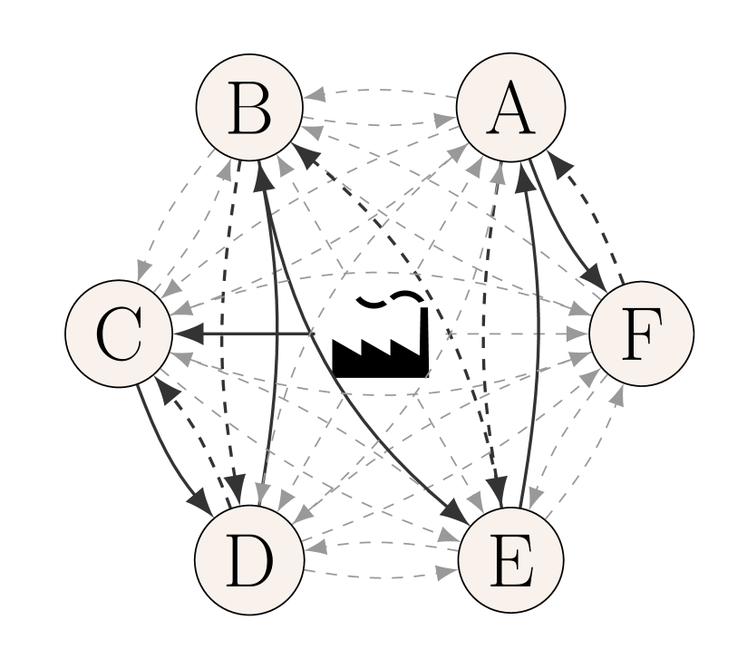
Scenario 1

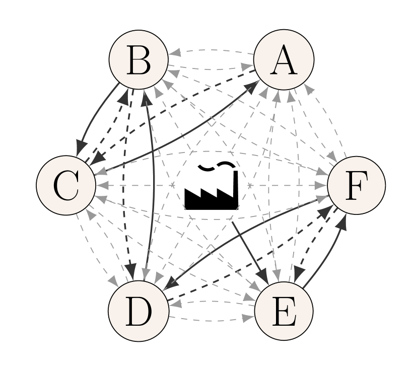
Scenario 2

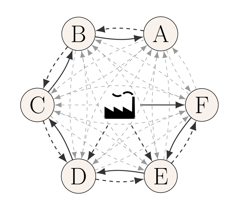
Scenario 3

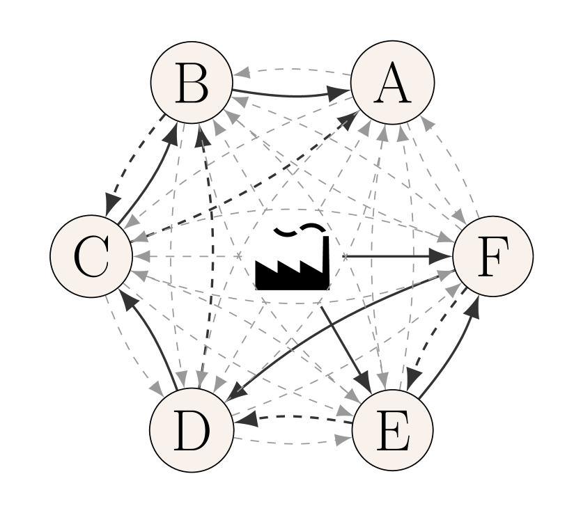
Target

(a) Transport cost visualization.

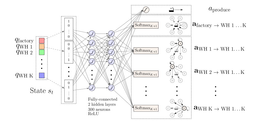
(b) Actor network.

Figure 4: Source and target task configuration and actor network used for the Supply Chain domain.

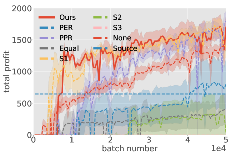
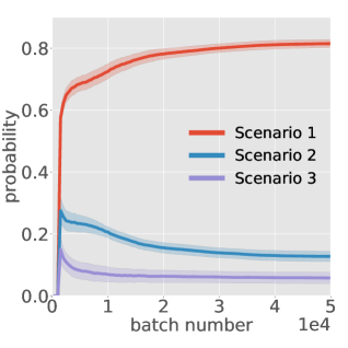
(a) Scenario 1

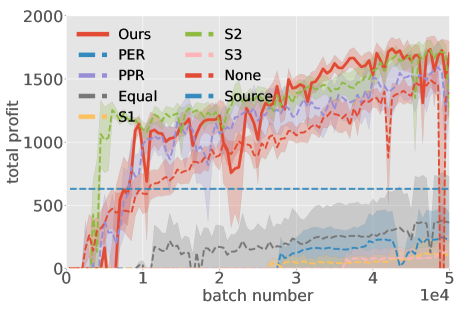
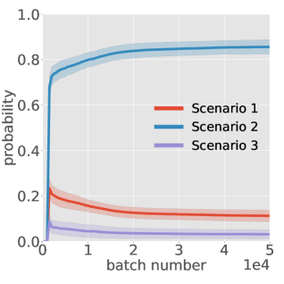
(b) Scenario 2

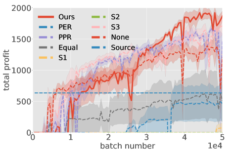
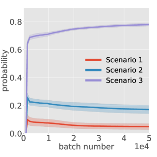
(c) Scenario 3

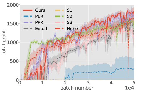
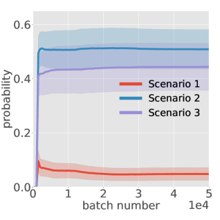
(d) Target Task

Figure 5: Total testing profit per episode (left) and weights assigned to source tasks (right) over epochs using soft pre-training of DDPG for the Supply Chain problem, with each source and target task as ground truth. Averaged over 5 trials with shaded standard error bars.

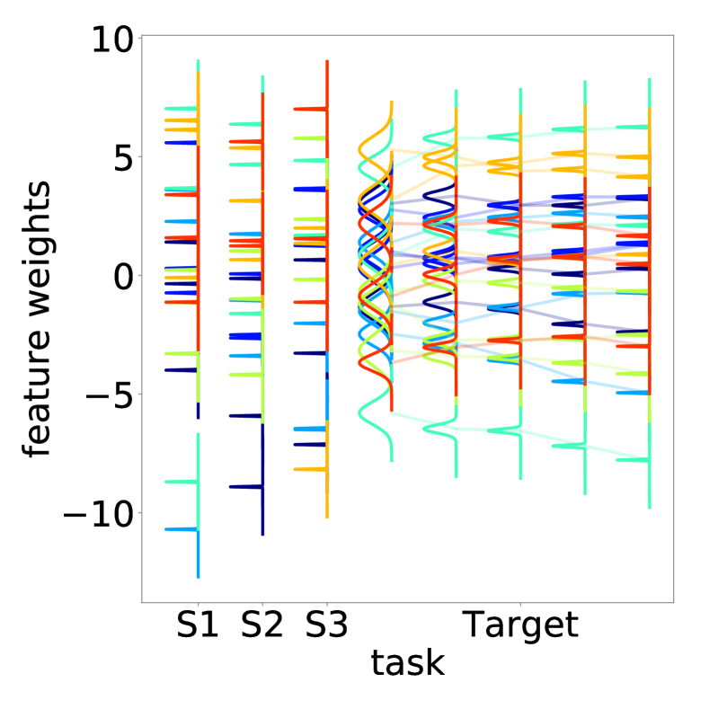
(a) Scenario 1

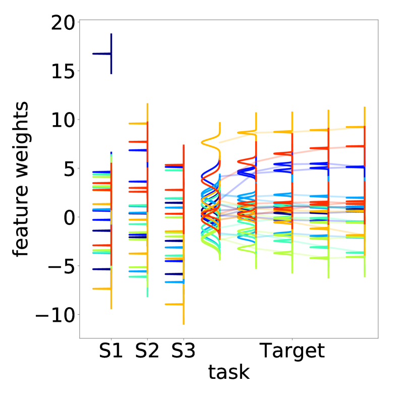
(b) Scenario 2

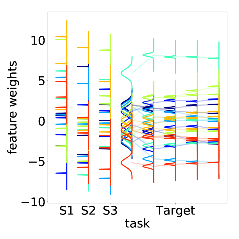
(c) Scenario 3

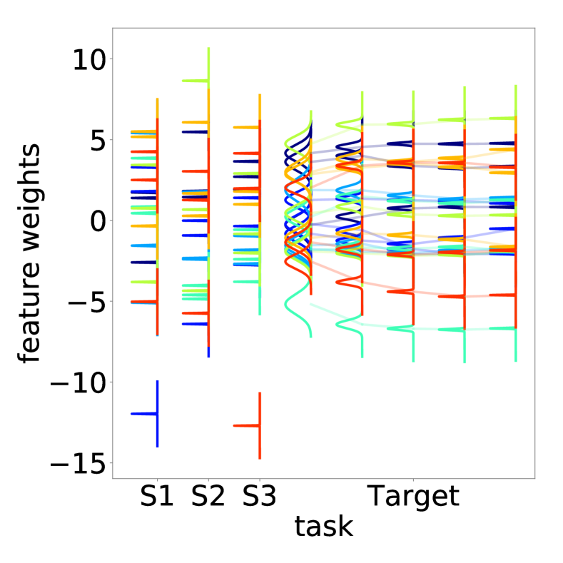
(d) Target

Figure 6: For Supply Chain control with each source and target task as the ground truth, shows the posterior marginal distributions of $\mathbf{w}_{i}$ and $\mathbf{w}_{target}$ during training on the target task (after 0, 10, 50, 100 and 200 episodes). Over time, the target features begin to concentrate on the corresponding values for the correct source task.

4.3 Discussion

On the optimization task, BERS achieves a small performance gap relative to the single best expert, since it can quickly identity the most suitable source task (Figure 2). While UCB is a strong baseline, BERS finds the solution in less iterations and with less variability. As expected, the QP solution favours the Sphere function as the source task when solving the Rastrigin function, because they are structurally similar functions, which leads to a quicker identification of the global minimum.

On the supply chain task, BERS also achieves results that are similar to the single best expert, and does better than PPR (while the asymptotic performance on Scenario 1 is similar, BERS achieves better jump-start performance). Both BERS and PPR are able to quickly surpass the performance of the exploration policy that generated the source data (shown as a horizontal line in Figure 5), whereas PER was not able to obtain satisfactory performance. We believe the latter is true because PER prioritizes experiences by TD error, which is not suitable when the rewards are sampled from different tasks, while BERS learns a common feature embedding to allow consistent comparison between tasks (Figure 3). We also believe that if the source data was considerably less optimal, then the performance gap between PPR and BERS would be greater. On the target scenario, it is interesting to see that the weights assigned to Scenarios 1 and 2 are roughly equal, which makes sense as the target task shares similarities with both scenarios (Figure 4(a)). By mixing two source tasks, BERS was able to perform substantially better on the target task than the two source tasks (S2 and S3) in isolation. Also by adopting a fully Bayesian treatment, we obtain smooth convergence of the task weights on all experiments.

5 Conclusion

We studied the problem of LfD with multiple sub-optimal demonstrators with different goals. To solve this problem, we proposed a multi-headed Bayesian neural network with a shared encoder to efficiently learn consistent representations of the source and target reward functions from the demonstrations. Reward functions were parameterized as linear models, whose uncertainty was modeled using Normal-Inverse-Gamma priors and updated using Bayes’ rule. A quadratic programming problem was formulated to rank the demonstrators while trading off the mean and variance of the uncertainty in the learned reward representations, and Bayesian Experience Reuse (BERS) was proposed to incorporate demonstrations directly when learning new tasks. Empirical results for static function optimization and RL suggest that our approach can successfully transfer experience from conflicting demonstrators in diverse tasks.

Broader Impact

This work presents a general framework for reusing demonstrations data available in general static and dynamic optimization problems. It could lead to positive societal consequences in terms of safety and reliability of automated systems, such as medical diagnosis systems that often require pre-training from human experts, or driver-less cars that learn from human mistakes to avoid similar situations in the real world, potentially saving lives in the process. On the other hand, because our approach requires the learning of the (latent) intentions of users and their goals, there could potentially be privacy concerns depending on how the trained agent decisions are implemented or published. This is particularly true shortly after commencement of training, when the learning agent can resemble one or more demonstrators in their decision making. Our framework is also based on deep learning methodologies, and so it naturally inherits some of the risks prevalent in that work (although our work also tries to address some of these issues by using a Bayesian approach). For example, data that consists of only exceptional situations (such as pre-training of a search and rescue robot), may consist of many outliers. Such data sets must sometimes undergo pre-processing to remove the effects of outliers or other features that could skew the algorithm and lead to the wrong conclusions. This could be catastrophic in mission critical operations where every decision counts. However, by using prudent machine learning practices, we believe the benefits of this work outweigh the risks.

Appendix

Hyper-Parameters for the Neural-Linear Model

We set $\mathbf{w}_{i}\sim\mathcal{N}(0,\mathbf{I})$, $\sigma_{i}^{2}\sim\mathrm{InvGamma}(1,1)$. For the encoder, we set $d=20$, use L2 regularization with penalty $\lambda=10^{-4}$, a learning rate of $10^{-4}$, and initialize weights using Glorot uniform. The encoder has two hidden layers with 200 ReLU units each (300 in the first layer for the supply chain problem), and $\tanh$ outputs. We also include a constant bias term in the feature map $\bm{\phi}$ when learning $\mathbf{w}$. Prior to transfer, we first train the neural linear model on 4000 batches of size 64 sampled uniformly from source data. During target training, we train on batches of size 64 sampled from source and target data after each iteration (generation for optimization, episode for supply chain) to avoid catastrophic forgetting of features (one batch for optimization and 20 for supply chain). QPs are solved from scratch at the end of each iteration using the cvxopt package [2].

Details for the Static Optimization Benchmark

Problem Setting:

The four test functions considered in this paper are as follows:

$$f_{Rosenbrock}(\mathbf{x}) =\sum_{i=1}^{D-1}100[(x_{i+1}-x_{i}^{2})^{2}+(1-x_{i})^{2}]$$

$$f_{Ackley}(\mathbf{x}) =-20\exp\left(-0.2\sqrt{\frac{1}{D}\sum_{i=1}^{D}x_{i}^{2}}\right)-\exp\left(\frac{1}{D}\sum_{i=1}^{D}\cos(2\pi x_{i})\right)+20+\exp{(1)}$$

$$f_{Sphere}(\mathbf{x}) =\sum_{i=1}^{D}(x_{i}+2)^{2}$$

$$f_{Rastrigin} =10D+\sum_{i=1}^{D}[(x_{i}+2)^{2}-10\cos(2\pi(x_{i}+2))],$$

where $\mathbf{x}=[x_{1},x_{2}\dots x_{D}]\in\mathbb{R}^{D}$ and restricted to $x_{i}\in[-4,4]$ for $i=1,2\dots D$ and we set $D=10$ for all experiments. The global minimums of the functions are, respectively, as follows: $x_{Rosenbrock}^{*}=\bm{1}_{D}$, $x_{Ackley}^{*}=\bm{0}_{D}$, $x_{Sphere}^{*}=-2\times\bm{1}_{D}$ and $x_{Rastrigin}^{*}=-2\times\bm{1}_{D}$. For Rosenbrock, Sphere and Rastrigin functions, we transform outputs using $y\mapsto\sqrt{y}$ so they become, approximately, equally scaled (for Rosenbrock we subsequently also divide by 10), to demonstrate whether we can actually “learn" each function from the data rather than distinguish it according to scale alone.

Solver Settings:

To optimize all functions, we use the Differential Evolution (DE) algorithm [41]. The pseudo-code of this algorithm is outlined in Algorithm 2.

Algorithm 2 Differential Evolution (DE)

0:  $f:\mathbb{R}^{D}\to\mathbb{R}$, $CR\in[0,1]$, $F\in[0,2]$, $NP\geq 4$

  initialize $NP$ points $\mathcal{P}$ uniformly at random in the search space

  for generation $m=1,2,\dots$ do

     for agent $\mathbf{x}\in\mathcal{P}$ do

        randomly select three candidates $\mathbf{a},\mathbf{b},\mathbf{c}\in\mathcal{P}$ that are distinct from each other and from $\mathbf{x}$

        pick a random index $R\in\{1,2\dots D\}$

        for $i=1,2\dots D$ do

           pick $r_{i}\sim U(0,1)$

           if $r_{i}<CR$ or $i=R$ then

              set $y_{i}=a_{i}+F(b_{i}-c_{i})$

           else

              set $y_{i}=x_{i}$

           end if

           if $f(\mathbf{y})\leq f(\mathbf{x})$ then

              replace $\mathbf{x}$ in $\mathcal{P}$ with $\mathbf{y}$

           end if

        end for

     end for

  end for

  return the agent in $\mathcal{P}$ with the least function value

Here, $CR$ is the crossover probability and denotes the probability of replacing a coordinate in an existing solution with the candidates (crossover), $F$ is the differential weight and controls the strength of the crossover, and $NP$ is the size of the population (larger implies a more global search). We use standard values $CR=0.7,F=0.5$ and $NP=32$ for reporting experimental results, unless indicated otherwise. The search bounds are also set to $[-4,+4]$ for all coordinates; all points that are generated during the initialization of the population and the crossover are clipped to this range.

Experimental Details:

We consider both transfer and multi-task learning settings. For the transfer experiment, we use the Rosenbrock, Ackley and Sphere functions as the source tasks, and the Rastrigin function as the target task. We also consider each of the source tasks as the ground truth to see whether we can identify the correct source task in an ideal controlled setting. In the multi-task setting, we did not observe any advantages of our algorithm nor the baselines when solving the Rosenbrock, Ackley or Sphere functions, so we focus on the quality of solution obtained for the Rastrigin function only. Transfer learning: We first generate demonstrations $(\mathbf{x}_{i},f(\mathbf{x}_{i}))$ from each source function $f$ using DE (Algorithm 2) and configuration above until a fitness of $0.15$ is achieved. Respectively, these have sizes 17693, 6452 and 5853 for each source task. We further transform outputs for training and prediction with the neural-linear model using a log-transform $y\mapsto\log(1+y)$ to limit the effects of outliers and stabilize the training of the model. When solving the target task, the batch $\mathcal{B}$ is a singleton set containing the best solution from the source data, and $O_{base}$ is trained by replacing the first of the three sampled candidates prior to crossover with probability $p_{m}=0.99^{m}$, where $m$ is the index of the current generation (following the structure of Algorithm 1). This guarantees that the new swarm will possess the traits of the source solutions with high probability, but still maintain diversity so the solution can be improved further. Multi-task learning: We solve all source and target functions simultaneously, sharing the best solutions between them using the mechanisms outlined above for the transfer learning experiment. One QP is maintained for each task to learn weightings over the other tasks excluding itself. Here, we set $p_{m}=0.3$, so that the best obtained solutions can be consistently shared between tasks over time.

Details for the Supply Chain Benchmark

Problem Setting:

Demand in units per time step is $d_{t,i}\sim\mathrm{Poisson}(\mu_{i})$, where $\mu_{i}$ is $\{7,6,6,5,5,5\}$ for warehouses (factory demand is zero) and is not backlogged but lost forever during shortages. The unit selling price is $0.6$, the unit production cost is $0.1$, the unit storage cost per time step is $0.03$ and the maximum storage capacity is capped at $50$ for the factory and each warehouse. A truck can ship only $4$ units, but the controller can dispatch an unlimited number of trucks from any location.

Solver Settings:

We use the Deep Deterministic Policy Gradient (DDPG) Algorithm [30] to solve this problem. The critic network has 300 hidden units per layer. We also use L2 penalty $\lambda=10^{-4}$, learning rates $10^{-4}$ and $2\times 10^{-4}$ for actor and critic respectively, $U(-3\times 10^{-3},3\times 10^{-3})$ initialization for weights in output layers, discount factor $\gamma=0.96$, horizon $T=200$, randomized replay with capacity $10000$, batch size of $32$, and explore using independent Gaussian noise $\mathcal{N}(0,\sigma_{t}^{2})$, where $\sigma_{t}$ is annealed from $0.15$ to $0$ linearly over $50000$ training steps.

Experimental Details:

We consider the transfer from multiple source tasks (Scenarios 1, 2 and 3) to a single target task (Target Task) as indicated in Figure 4(a). We also consider each source task as a ground truth. To collect source data, we train DDPG with the above hyper-parameters on each source task for $30000$ time steps, then randomly sub-sample $10000$ observations. This last step demonstrates whether our approach can learn stable representations with limited data and incomplete exploration trajectories. Since regression is sensitive to outliers, when training the neural linear model, we remove $2.5\%$ of the samples with the highest and lowest rewards (we also exclude observations collected from the target task that lie outside any of these bounds). In order to implement transfer, we set $p_{m}=0.95^{m}$, where $m$ is the current episode number. This provides a reasonable balance between exploration of source data and exploitation of target data. In accordance with Algorithm 1, we sample batches $\mathcal{B}$ of size 32 uniformly at random from the source data.

Details for Prioritized Experience Replay

Experimental Details:

We evaluated the performance of Prioritized Experience Replay [39] (PER) on the Supply Chain benchmark. In summary, PER is a replay buffer that ranks experiences using the Bellman error, defined for the DDPG algorithm for a transition $(s,a,r,s^{\prime})$ as

$$\delta=r+\gamma Q^{\prime}(s^{\prime},\mu^{\prime}(s^{\prime}))-Q(s,a),$$

where $Q$ is the critic network, and $Q^{\prime}$ and $\mu^{\prime}$ are the target critic and target actor networks, respectively.

In order to use PER to transfer experiences, we load all source demonstrations into the replay buffer prior to target task training with initial Bellman error $\delta=1$. The source demonstrations are first combined into a single data set and shuffled. The capacity of the buffer is then fixed to the total number of source demonstrations from all tasks (around 28,000 examples). During target training, observed transitions are immediately added to the replay buffer and override the oldest experience. In this way, the agent is able to maximize the use of the source data at the beginning of training but eventually shift emphasis to target task data.

Detailed Analysis:

Figure 7 demonstrates the composition of each batch (of size 32) according to source (Scenario 1, Scenario 2, Scenario 3, Target Task) for each ground truth. As illustrated in all four plots, in early stages of training, batches are predominantly composed of source data, while in later stages, they consist entirely of target data. Figure 7 shows that PER is unable to favor demonstrations from the source task that correspond to the ground truth, in all four problem settings. One possible explanation of this is that an implicit assumption of PER is violated, namely that experiences are drawn from the same distribution of rewards, whereas in our experiment, experiences can come from tasks with contradictory goals. In this case, experiences corresponding to the ground truth do not necessarily have larger Bellman error (in fact, the opposite may be true).

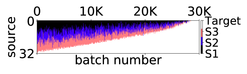
(a) Scenario 1

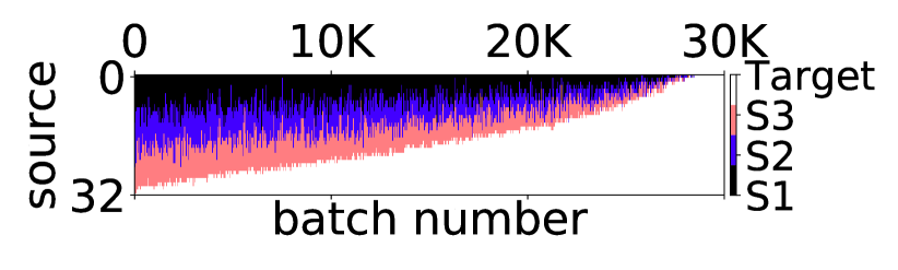
(b) Scenario 2

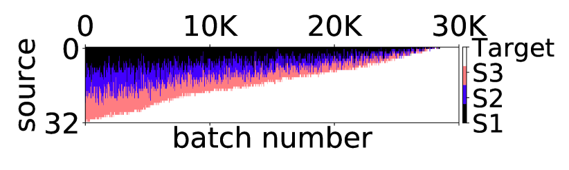
(c) Scenario 3

(d) Scenario 4

Figure 7: Shows the composition of each batch over time sampled from the prioritized replay (PER) according to whether the sample came from the source or target task data, for each ground truth. PER is unable to rank experiences correctly to match the context.

References

- Amos and Kolter [2017] Brandon Amos and J Zico Kolter. Optnet: Differentiable optimization as a layer in neural networks. In International Conference on Machine Learning, pages 136–145. JMLR. org, 2017.
- Andersen et al. [2015] M Andersen, J Dahl, and L Vandenberghe. Cvxopt: Python software for convex optimization, version 1.1, 2015.
- Argall et al. [2009] Brenna D Argall, Sonia Chernova, Manuela Veloso, and Brett Browning. A survey of robot learning from demonstration. Robotics and autonomous systems, 57(5):469–483, 2009.
- Auer [2002] Peter Auer. Using confidence bounds for exploitation-exploration trade-offs. Journal of Machine Learning Research, 3(Nov):397–422, 2002.
- Azizsoltani et al. [2019] Hamoon Azizsoltani, Yeo Jin Kim, Markel Sanz Ausin, Tiffany Barnes, and Min Chi. Unobserved is not equal to non-existent: using gaussian processes to infer immediate rewards across contexts. In Proceedings of the 28th International Joint Conference on Artificial Intelligence, pages 1974–1980. AAAI Press, 2019.
- Barreto et al. [2017] André Barreto, Will Dabney, Rémi Munos, Jonathan J Hunt, Tom Schaul, Hado P van Hasselt, and David Silver. Successor features for transfer in reinforcement learning. In Advances in Neural Information Processing Systems, pages 4055–4065, 2017.
- Barreto et al. [2018] Andre Barreto, Diana Borsa, John Quan, Tom Schaul, David Silver, Matteo Hessel, Daniel Mankowitz, Augustin Zidek, and Remi Munos. Transfer in deep reinforcement learning using successor features and generalised policy improvement. In International Conference on Machine Learning, pages 501–510, 2018.
- Bishop [2006] Christopher M Bishop. Pattern recognition and machine learning. springer, 2006.
- Bojarski et al. [2016] Mariusz Bojarski, Davide Del Testa, Daniel Dworakowski, Bernhard Firner, Beat Flepp, Prasoon Goyal, Lawrence D Jackel, Mathew Monfort, Urs Muller, Jiakai Zhang, et al. End to end learning for self-driving cars. arXiv preprint arXiv:1604.07316, 2016.
- Bouzerdoum and Pattison [1993] Abdesselam Bouzerdoum and Tim R Pattison. Neural network for quadratic optimization with bound constraints. IEEE Transactions on Neural Networks, 4(2):293–304, 1993.
- Boyd et al. [2004] Stephen Boyd, Stephen P Boyd, and Lieven Vandenberghe. Convex optimization. Cambridge university press, 2004.
- Brown et al. [2020] Daniel S. Brown, Russell Coleman, Ravi Srinivasan, and Scott Niekum. Safe imitation learning via fast bayesian reward inference from preferences, 2020.
- Brys et al. [2015] Tim Brys, Anna Harutyunyan, Halit Bener Suay, Sonia Chernova, Matthew E Taylor, and Ann Nowé. Reinforcement learning from demonstration through shaping. In Twenty-Fourth International Joint Conference on Artificial Intelligence, 2015.
- Chernova and Thomaz [2014] Sonia Chernova and Andrea L Thomaz. Robot learning from human teachers. Synthesis Lectures on Artificial Intelligence and Machine Learning, 8(3):1–121, 2014.
- Cruz Jr et al. [2017] Gabriel V Cruz Jr, Yunshu Du, and Matthew E Taylor. Pre-training neural networks with human demonstrations for deep reinforcement learning. arXiv preprint arXiv:1709.04083, 2017.
- Fernández et al. [2010] Fernando Fernández, Javier García, and Manuela Veloso. Probabilistic policy reuse for inter-task transfer learning. Robotics and Autonomous Systems, 58(7):866–871, 2010.
- Ferreau et al. [2008] Hans Joachim Ferreau, Hans Georg Bock, and Moritz Diehl. An online active set strategy to overcome the limitations of explicit mpc. International Journal of Robust and Nonlinear Control: IFAC-Affiliated Journal, 18(8):816–830, 2008.
- Flet-Berliac and Preux [2019] Yannis Flet-Berliac and Philippe Preux. Merl: Multi-head reinforcement learning. In NeurIPS 2019-Deep Reinforcement Learning Workshop, 2019.
- Gao et al. [2018] Yang Gao, Huazhe Xu, Ji Lin, Fisher Yu, Sergey Levine, and Trevor Darrell. Reinforcement learning from imperfect demonstrations. arXiv preprint arXiv:1802.05313, 2018.
- Gimelfarb et al. [2018] Michael Gimelfarb, Scott Sanner, and Chi-Guhn Lee. Reinforcement learning with multiple experts: A bayesian model combination approach. In Advances in Neural Information Processing Systems, pages 9528–9538, 2018.
- Grollman and Billard [2011] Daniel H Grollman and Aude Billard. Donut as i do: Learning from failed demonstrations. In 2011 IEEE International Conference on Robotics and Automation, pages 3804–3809. IEEE, 2011.
- Hester et al. [2018] Todd Hester, Matej Vecerik, Olivier Pietquin, Marc Lanctot, Tom Schaul, Bilal Piot, Dan Horgan, John Quan, Andrew Sendonaris, Ian Osband, et al. Deep q-learning from demonstrations. In Thirty-Second AAAI Conference on Artificial Intelligence, 2018.
- Hou et al. [2017] Yuenan Hou, Lifeng Liu, Qing Wei, Xudong Xu, and Chunlin Chen. A novel ddpg method with prioritized experience replay. In 2017 IEEE International Conference on Systems, Man, and Cybernetics (SMC), pages 316–321. IEEE, 2017.
- Jamil and Yang [2013] Momin Jamil and Xin-She Yang. A literature survey of benchmark functions for global optimisation problems. International Journal of Mathematical Modelling and Numerical Optimisation, 4(2):150–194, 2013.
- Janz et al. [2019] David Janz, Jiri Hron, Przemysław Mazur, Katja Hofmann, José Miguel Hernández-Lobato, and Sebastian Tschiatschek. Successor uncertainties: exploration and uncertainty in temporal difference learning. In Advances in Neural Information Processing Systems, pages 4509–4518, 2019.
- Konda and Tsitsiklis [2000] Vijay R Konda and John N Tsitsiklis. Actor-critic algorithms. In Advances in Neural Information Processing Systems, pages 1008–1014, 2000.
- Li et al. [2018] Guohao Li, Matthias Mueller, Vincent Casser, Neil Smith, Dominik L Michels, and Bernard Ghanem. Oil: Observational imitation learning. arXiv preprint arXiv:1803.01129, 2018.
- Li and Kudenko [2018] Mao Li and D Kudenko. Reinforcement learning from multiple experts demonstrations. In Workshop on Adaptive Learning Agents (ALA) at the Federated AI Meeting, volume 18, 2018.
- Li and Zhang [2018] Siyuan Li and Chongjie Zhang. An optimal online method of selecting source policies for reinforcement learning. In Thirty-Second AAAI Conference on Artificial Intelligence, 2018.
- Lillicrap et al. [2015] Timothy P Lillicrap, Jonathan J Hunt, Alexander Pritzel, Nicolas Heess, Tom Erez, Yuval Tassa, David Silver, and Daan Wierstra. Continuous control with deep reinforcement learning. arXiv preprint arXiv:1509.02971, 2015.
- Mnih et al. [2015] Volodymyr Mnih, Koray Kavukcuoglu, David Silver, Andrei A Rusu, Joel Veness, Marc G Bellemare, Alex Graves, Martin Riedmiller, Andreas K Fidjeland, Georg Ostrovski, et al. Human-level control through deep reinforcement learning. Nature, 518(7540):529–533, 2015.
- Nicolescu and Mataric [2003] Monica N Nicolescu and Maja J Mataric. Natural methods for robot task learning: Instructive demonstrations, generalization and practice. In Proceedings of the second international joint conference on Autonomous agents and multiagent systems, pages 241–248, 2003.
- Pardoe and Stone [2010] David Pardoe and Peter Stone. Boosting for regression transfer. In Proceedings of the 27th International Conference on Machine Learning, pages 863–870, 2010.
- Perrone et al. [2018] Valerio Perrone, Rodolphe Jenatton, Matthias W Seeger, and Cédric Archambeau. Scalable hyperparameter transfer learning. In Advances in Neural Information Processing Systems, pages 6845–6855, 2018.
- Powell [2007] Warren B Powell. Approximate Dynamic Programming: Solving the curses of dimensionality, volume 703. John Wiley & Sons, 2007.
- Price and Boutilier [2003] Bob Price and Craig Boutilier. A bayesian approach to imitation in reinforcement learning. In Twenty-Fourth International Joint Conference on Artificial Intelligence, pages 712–720, 2003.
- Puterman [2014] Martin L Puterman. Markov decision processes: discrete stochastic dynamic programming. John Wiley & Sons, 2014.
- Schaal [1997] Stefan Schaal. Learning from demonstration. In Advances in Neural Information Processing Systems, pages 1040–1046, 1997.
- Schaul et al. [2015] Tom Schaul, John Quan, Ioannis Antonoglou, and David Silver. Prioritized experience replay. arXiv preprint arXiv:1511.05952, 2015.
- Snoek et al. [2015] Jasper Snoek, Oren Rippel, Kevin Swersky, Ryan Kiros, Nadathur Satish, Narayanan Sundaram, Mostofa Patwary, Mr Prabhat, and Ryan Adams. Scalable bayesian optimization using deep neural networks. In International Conference on Machine Learning, pages 2171–2180, 2015.
- Storn and Price [1997] Rainer Storn and Kenneth Price. Differential evolution–a simple and efficient heuristic for global optimization over continuous spaces. Journal of Global Optimization, 11(4):341–359, 1997.
- Suay et al. [2016] Halit Bener Suay, Tim Brys, Matthew E Taylor, and Sonia Chernova. Learning from demonstration for shaping through inverse reinforcement learning. In Proceedings of the 2016 International Conference on Autonomous Agents & Multiagent Systems, pages 429–437, 2016.
- Sutton and Barto [2018] Richard S Sutton and Andrew G Barto. Reinforcement learning: An introduction. MIT press, 2018.
- Sutton et al. [2000] Richard S Sutton, David A McAllester, Satinder P Singh, and Yishay Mansour. Policy gradient methods for reinforcement learning with function approximation. In Advances in Neural Information Processing Systems, pages 1057–1063, 2000.
- Taylor et al. [2011] Matthew E Taylor, Halit Bener Suay, and Sonia Chernova. Integrating reinforcement learning with human demonstrations of varying ability. In The 10th International Conference on Autonomous Agents and Multiagent Systems, pages 617–624, 2011.
- Thakur et al. [2019] Sanjay Thakur, Herke van Hoof, Juan Camilo Gamboa Higuera, Doina Precup, and David Meger. Uncertainty aware learning from demonstrations in multiple contexts using bayesian neural networks. In 2019 International Conference on Robotics and Automation (ICRA), pages 768–774. IEEE, 2019.
- van Lent and Laird [2001] Michael van Lent and John E Laird. Learning procedural knowledge through observation. In Proceedings of the 1st international conference on Knowledge capture, pages 179–186, 2001.
- Van Seijen et al. [2017] Harm Van Seijen, Mehdi Fatemi, Joshua Romoff, Romain Laroche, Tavian Barnes, and Jeffrey Tsang. Hybrid reward architecture for reinforcement learning. In Advances in Neural Information Processing Systems, pages 5392–5402, 2017.
- Vezzani et al. [2019] Giulia Vezzani, Abhishek Gupta, Lorenzo Natale, and Pieter Abbeel. Learning latent state representation for speeding up exploration. arXiv preprint arXiv:1905.12621, 2019.
- Wang et al. [2019] Boyu Wang, Jorge Mendez, Mingbo Cai, and Eric Eaton. Transfer learning via minimizing the performance gap between domains. In Advances in Neural Information Processing Systems, pages 10644–10654, 2019.
- Wang and Taylor [2017] Zhaodong Wang and Matthew E Taylor. Improving reinforcement learning with confidence-based demonstrations. In Twenty-Sixth International Joint Conference on Artificial Intelligence, pages 3027–3033, 2017.
- Watkins and Dayan [1992] Christopher JCH Watkins and Peter Dayan. Q-learning. Machine Learning, 8(3-4):279–292, 1992.
- Yao and Doretto [2010] Yi Yao and Gianfranco Doretto. Boosting for transfer learning with multiple sources. In 2010 IEEE Computer Society Conference on Computer Vision and Pattern Recognition, pages 1855–1862. IEEE, 2010.