Hypergraph Clustering for Finding
Diverse and Experienced Groups

Abstract

When forming a team or group of individuals, we often seek a balance of expertise in a particular task while at the same time maintaining diversity of skills within each group. Here, we view the problem of finding diverse and experienced groups as clustering in hypergraphs with multiple edge types. The input data is a hypergraph with multiple hyperedge types — representing information about past experiences of groups of individuals — and the output is groups of nodes. In contrast to related problems on fair or balanced clustering, we model diversity in terms of variety of past experience (instead of, e.g., protected attributes), with a goal of forming groups that have both experience and diversity with respect to participation in edge types. In other words, both diversity and experience are measured from the types of the hyperedges.

Our clustering model is based on a regularized version of an edge-based hypergraph clustering objective, and we also show how naive objectives actually have no diversity-experience tradeoff. Although our objective function is NP-hard to optimize, we design an efficient 2-approximation algorithm and also show how to compute bounds for the regularization hyperparameter that lead to meaningful diversity-experience tradeoffs. We demonstrate an application of this framework in online review platforms, where the goal is to curate sets of user reviews for a product type. In this context, “experience” corresponds to users familiar with the type of product, and “diversity” to users that have reviewed related products.

1 Introduction

Team formation within social and organizational contexts is ubiquitous in modern society, as success often relies on forming the “right” teams. Diversity within these teams, both with respect to socioeconomic attributes and expertise across disciplines, often leads to synergy, and brings fresh perspectives which facilitate innovation. The study of diverse team formation with respect to expertise has a rich history spanning decades of work in sociology, psychology and business management [21, 24, 26, 33]. In this paper, we explore algorithmic approaches to diverse team formation, where “diversity” corresponds to a group of individuals with a variety of experiences. In particular, we present a new algorithmic framework for diversity in clustering that focuses on forming groups which are diverse and experienced in terms of past group interactions. As a motivating example, consider a diverse team formation task in which the goal is to assign a task to a group of people who (1) already have some level of experience working together on the given task, and (2) are diverse in terms of their previous work experience. As another example, a recommender system may want to display a diverse yet cohesive set of reviews for a certain class of products. In other words, the set of displayed reviews should work well together in providing an accurate overview of the product category.

Here, we formalize diverse and experienced group formation as a clustering problem on edge-labeled hypergraphs. In this setup, a hyperedge represents a set of objects (such as a group of individuals) that have participated in a group interaction or experience. The hyperedge label encodes the type or category of interaction (e.g., a type of team project). The output is then a labeled clustering of nodes, where cluster labels are chosen from the set of hyperedge labels. The goal is to form clusters whose nodes are balanced in terms of experience and diversity. By experience we mean that a cluster with label $\ell$ should contain nodes that have previously participated in hyperedges of label $\ell$. By diversity, we mean that clusters should also include nodes that have participated in other hyperedge types.

Our mathematical framework for diverse and experienced clustering builds on an existing objective for clustering edge-labeled hypergraphs [5]. This objective encourages cluster formation in such a way that hyperedges of a certain label tend to be contained in a cluster with the same label, similar to (chromatic) correlation clustering [7, 11]. We add a regularization term to this objective that encourages clusters to contain nodes that have participated in many different hyperedge types. This diversity-encouraging regularization is governed by a tunable parameter $\beta\geq 0$, where $\beta=0$ corresponds to the original edge-labeled clustering objective. Although the resulting objective is NP-hard in general, we design a linear programming algorithm that guarantees a 2-approximation for any choice of $\beta$. We show that certain values of this hyperparameter reduce to extremal solutions with closed-form solutions where just diversity or just experience is encouraged. In order to guide a meaningful hyperparameter selection, we show how to bound the region in which non-extremal solutions occur, leveraging linear programming sensitivity techniques.

We demonstrate the utility of our framework by applying it to team formation of users posting answers on Stack Overflow, and the task of aggregating a diverse set of reviews for categories of establishments and products on review sites (e.g., Yelp or Amazon). We find that the framework yields meaningfully more diverse clusters at a small cost in terms of the unregularized objective, and the approximation algorithms we develop produce solutions within a factor of no more than 1.3 of optimality empirically. A second set of experiments examines the effect of iteratively applying the diversity-regularized objective while keeping track of the experience history of every individual. We observe in this synthetic setup that regularization greatly influences team formation dynamics over time, with more frequent role swapping as regularization strength increases.

1.1 Related work

Our work on diversity in clustering is partly related to the recent research on algorithmic fairness and fair clustering, which we briefly review. These results are based ideas that machine learning algorithms may make decisions that are biased or unfair towards a subset of a population [8, 17, 18]. There are now a variety of algorithmic fairness techniques to combat this issue [19, 28, 37]. For clustering problems, fairness is typically formulated in terms of protected attributes on data points — a cluster is “fair” if it exhibits a proper balance between nodes from different protected classes, and the goal is to optimize classical clustering objectives while also adhering to constraints ensuring a balance on the protected attributes [2, 4, 3, 10, 15, 16, 20, 30]. These approaches are similar to our notion of diverse clustering, since in both cases, the resulting clusters are more heterogeneous with respect to node attributes. While the primary attribute addressed in fair clustering is the protected status of a data point, in our case it is the “experience” of that point, which is derived from an edge-labeled hypergraph. In this sense, we have similar algorithmic goals, but we present our approach as a general framework for finding clusters of nodes with experience and diversity, as there are many reasons why one may wish to organize a dataset into clusters that are diverse with respect to past experience.

Furthermore, there exists some literature on algorithmic diverse team formation [6, 13, 29, 36, 41, 45]. However, this research has thus far largely focused on frameworks for forming teams which exhibit diversity with respect to inherent node-level attributes, without an emphasis on diversity of expertise, making our work the first to explicitly address this issue.

Our framework also facilitates a novel take on diversity within recommender systems. A potential application which we study in Section 4 is to select expert, yet diverse sets of reviews for different product categories. This differs from existing recommender systems paradigms on two fronts: First, the literature focuses almost exclusively on user-centric recommendations, with content tailored to an individual’s preferences; for us, a set of reviews is curated for a category of products that allows any user to glean both expert and diverse opinions regarding it. Further, the classic recommender systems literature defines diversity for a set of objects based on dissimilarity derived from pairwise relations among people and objects [12, 31, 35, 43, 46]. While some set-level proxies for diverse recommendations exist [14, 40], they do not deal explicitly with higher-order interactions among objects. Our work, on the other hand, encourages diversity in recommendations through an objective that captures higher-order information about relations between subsets of objects, providing a native framework for hypergraph-based diverse recommendations.

2 Forming Clusters Based on Diversity and Experience

We first introduce notation for edge-labeled clustering. After, we analyze an approach that seems natural for clustering based on experience and diversity, but leads only to trivial solutions. We then show how a regularized version of a previous hypergraph clustering framework leads to a more meaningful objective, which will be the focus of the remainder of the paper.

Notation.  Let $G=(V,E,L,\ell)$ be a hypergraph with labeled edges, where $V$ is the set of nodes, $E$ is the set of (hyper)edges, $L$ is a set of edge labels, and $\ell\colon E\rightarrow L$ maps edges to labels, where $L=\{1,\ldots,k\}$ and $k$ is the number of labels. Furthermore, let $E_{c}\subseteq E$ be the edges with label $c$, and $r$ the maximum hyperedge size. Following graph-theoretic terminology, we often refer to elements in $L$ as “colors”; in data, $L$ represents categories or types. For any node $v\in V$, let $d_{v}^{c}$ be the number of hyperedges of color $c$ in which node $v$ appears. We refer to $d_{v}^{c}$ as the color degree of $v$ for color $c$.

Given this input, an algorithm will output a color for each node. Equivalently, this is a clustering $\mathcal{C}$, where each node is assigned to exactly one cluster, and there is exactly one cluster for each color in $L$. We use $\mathcal{C}(i)$ to denote the nodes assigned to color $i\in L$. We wish to find a clustering that promotes both diversity (clusters have nodes from a range of colored hyperedges), and experience (a cluster with color $c$ contains nodes that have experience participating in hyperedges of color $c$).

2.1 A flawed but illustrative first approach

We start with an illustrative (but ultimately flawed) clustering objective whose characteristics will be useful in the rest of the paper. For this, we first define diversity and experience scores for a color $i$, denoted $D(i)$ and $E(i)$, as follows:

$$D(i)=\sum_{v\in\mathcal{C}(i),c\neq i}d_{v}^{c}\,,\hskip 14.22636ptE(i)=\sum_{v\in\mathcal{C}(i)}d_{v}^{i}.$$ (1)

In words, $D(i)$ measures how much nodes in cluster $i$ have participated in hyperedges that are not color $i$, and $E(i)$ measures how much nodes in cluster $i$ have participated in hyperedges of color $i$. A seemingly natural but ultimately naive objective for balancing experience and diversity is:

$$\max_{\mathcal{C}}\sum_{i\in L}[E(i)+\beta D(i)].$$ (2)

The regularization parameter $\beta$ determines the relative importance of the diversity and experience scores. It turns out that the optimal solutions to this objective are overly-simplistic, with a phase transition at $\beta=1$. We define two simple types of clusterings as follows:

• Majority vote clustering: Node $v$ is placed in cluster $\mathcal{C}(i)$ where $i\in\operatorname{argmax}_{c\in L}d_{v}^{c}$, i.e., node $v$ is placed in a cluster for which it has the most experience.

• Minority vote clustering: Node $v$ is placed in cluster $\mathcal{C}(i)$ where $i\in\operatorname{argmin}_{c\in L}d_{v}^{c}$, i.e., node $v$ is placed in a cluster for which it has the least experience.

The following theorem explains why (1) does not provide a meaningful tradeoff between diversity and experience.

Theorem 1

A majority vote clustering optimizes (2) for all $\beta>1$, and a minority vote clustering optimizes the same objective for all $\beta<1$. Both are optimal when $\beta=1$.

Proof  For node $i$, assume without loss of generality that the colors $1,2,\ldots,k$ are ordered so that $d_{i}^{1}\geq\dots\geq d_{i}^{k}$. Clustering $i$ with cluster 1 gives a contribution of $d_{i}^{1}+\beta\sum_{j=2}^{k}d_{i}^{j}$ to the objective, while clustering it with color $c\neq i$ gives contribution $d_{i}^{c}+\beta\sum_{j\neq c}d_{i}^{j}$. Because $d_{i}^{1}\geq\dots\geq d_{i}^{k}$, the first contribution is greater than or equal to the second if and only if $\beta\leq 1$. Hence, majority vote is optimal when $\beta\geq 1$. A similar argument proves optimality for minority vote when $\beta\leq 1$. $\Box$

Objective (2) is easy to analyze, but has optimal points that do not provide a balance between diversity and experience. This occurs because a clustering will maximize the total diversity $\sum_{c\in L}D(c)$ if and only if it minimizes the total experience $\sum_{c\in L}E(c)$, as these terms sum to a constant. We formalize this in the following observation.

Observation 2

$\sum_{c\in L}[E(c)+D(c)]$ is a constant independent of the clustering $\mathcal{C}$.

We will use this observation when developing our clustering framework in the next section.

2.2 Diversity-regularized categorical edge clustering

We now turn to a more sophisticated approach: a regularized version of the categorical edge clustering objective [5]. For a clustering $\mathcal{C}$, the objective accumulates a penalty of 1 for each hyperedge of color $c$ that is not completely contained in the cluster $\mathcal{C}(c)$. More formally, the objective is:

$$\min_{\mathcal{C}}\sum_{c\in L}\sum_{e\in E_{c}}x_{e},$$ (3)

where $x_{e}$ is an indicator variable equal to 1 if hyperedge $e\in E_{c}$ is not contained in cluster $\mathcal{C}(c)$, but is zero otherwise. This penalty encourages entire hyperedges to be contained inside clusters of the corresponding color. For our context, this objective can be interpreted as promoting group experience in cluster formation: if a group of people have participated together in task $c$, this is an indication they could work well together on task $c$ in the future. However, we want to avoid the scenario where groups of people endlessly work on the same type of task without the benefiting from the perspective of others with different experiences. Therefore, we regularize objective (3) with a penalty term $\beta\sum_{c\in L}E(c)$. Since $\sum_{c\in L}[E(c)+D(c)]$ is a constant (Observation 2), this regularization encourages higher diversity scores $D(c)$ for each cluster $\mathcal{C}(c)$.

While the “all-or-nothing” penalty in (3) may seem restrictive at first, it is a natural choice for our objective function for several reasons. First, we are building on recent research showing applications of Objective (3) on datasets similar to ours, namely edge-labeled hypergraphs [5], and this type of penalty is a standard in hypergraph partitioning [9, 23, 25, 34, 32, 42]. Second, if we consider an alternative penalty which incurs a cost of one for every node that is split away from the color of the hyperedge, this reduces to the “flawed first approach” in the previous section, where there is no diversity-experience tradeoff. Developing algorithms that can optimize more complicated alternative hyperedge cut penalties is an active area of research [34, 44]. Translating these ideas to our setting constitutes an interesting open direction for future work, but comes with numerous challenges and is not the focus of the current manuscript. Finally, our experimental results indicate that even without considering generalized hyperedge cut penalties, our regularized objective produces meaningfully diverse clusters on real-world and synthetic data.

We now formalize our objective function, which we call diversity-regularized categorical edge clustering (DRCEC), which will be the focus for the remainder of the paper. We state the objective as an integer linear program (ILP):

$$\begin{array}[]{lll}\min&\sum_{c\in L}\sum_{e\in E_{c}}x_{e}+\beta\sum_{v\in V}\sum_{c\in L}d_{v}^{c}(1-x_{v}^{c})&\\[2.84526pt] \text{s.t.}&\text{for all $v\in V$:}\;\sum_{c=1}^{k}x_{v}^{c}=k-1,&\\ &\text{for all $c\in L$, $e\in E_{c}$:}\;x_{v}^{c}\leq x_{e}\text{ for all $v\in e$};\\ &\text{for all $c\in L$, $v\in V$, $e\in E$:}\;x_{v}^{c},x_{e}\in\{0,1\}.\end{array}$$ (4)

The binary variable $x_{v}^{c}$ equals $1$ if node $v$ is not assigned label $c$, and is 0 otherwise. The first constraint guarantees every node is assigned to exactly one color, while the second constraint guarantees that if a single node $v\in e$ is not assigned to the cluster of the color of $e$, then $x_{e}=1$.

A polynomial-time 2-approximation algorithm.  Optimizing the case of $\beta=0$ is NP-hard [5], so DRCEC is also NP-hard. Although the optimal solution to (4) may vary with $\beta$, we develop a simple algorithm based on solving an LP relaxation of the ILP that rounds to a 2-approximation for every value of $\beta$. Our LP relaxation of the ILP in (4) replaces the binary constraints $x_{v}^{c},x_{e}\in\{0,1\}$ with linear constraints $x_{v}^{c},x_{e}\in[0,1]$. The LP can be solved in polynomial time, and the objective score is a lower bound on the optimal solution score to the NP-hard ILP. The values of $x_{v}^{c}$ can then be rounded into integer solutions to produce a clustering that is within a bounded factor of the LP lower bound, and therefore within a bounded factor of optimality. Our algorithm is simply stated:

$\begin{array}[]{l}\textbf{\text@underline{Algorithm 1}}\vspace{0.5mm}\\ \text{1. Solve the LP relaxation of the ILP in \eqref{eq:ccilp}.}\\ \text{2. For each $v\in V$, assign $v$ to any $c\in\operatorname{argmin}_{j}x_{v}^{j}$.}\end{array}$

The following theorem shows that the LP relaxation is a 2-approximation for the ILP formulation of the DRCEC objective.

Theorem 3

For any $\beta\geq 0$, Algorithm 1 returns a 2-approximation for objective (4).

Proof  Let the relaxed solution be $\{x_{e}^{*},x_{v}^{*c}\}_{e\in E,v\in V,c\in L}$ and the corresponding rounded solution $\{x_{e},x_{v}^{c}\}_{e\in E,v\in V,c\in L}$. Let $y_{v}^{c}=1-x_{v}^{c}$ and $y_{v}^{*c}=1-x_{v}^{*c}$. Our objective evaluated at the relaxed and rounded solutions respectively are

$$S^{*} =\sum_{e}x_{e}^{*}+\beta\sum_{v\in V}\sum_{c\in L}d_{v}^{c}y_{v}^{*c}\text{ and }$$

$$S =\sum_{e}x_{e}+\beta\sum_{v\in V}\sum_{c\in L}d_{v}^{c}y_{v}^{c}.$$

We will show that $S\leq 2S^{*}$ by comparing the first and second terms of $S$ and $S^{*}$ respectively. The first constraint in (4) ensures that $x_{v}^{c}<1/2$ for at most a single color $c$. Thus, for every edge $e$ with $x_{e}=1$, $x_{v}^{*c}\geq 1/2$ for some $v\in e$. In turn, $x_{e}^{*}\geq 1/2$, so $x_{e}\leq 2x_{e}^{*}$. If $x_{e}=0$, then $x_{e}\leq 2x_{e}^{*}$ holds trivially. Thus, $\sum_{e}x_{e}\leq 2\sum_{e}x_{e}^{*}$. Similarly, since $x_{v}^{c}=1$ ($y_{v}^{c}=0$) if and only if $x_{v}^{*c}\geq 1/2$ ($y_{v}^{c*}\leq 1/2$), and $x_{v}^{c}=0$ otherwise, it follows that $y_{v}^{c}\leq 2y_{v}^{*c}$. Thus, $\sum_{v\in V}\sum_{c\in L}d_{v}^{c}y_{v}^{c}\leq 2\sum_{v\in V}\sum_{c\in L}d_{v}^{c}y_{v}^{*c}$. $\Box$

2.3 Extremal LP and ILP solutions at large enough values of $\beta$

In general, Objective (4) provides a meaningful way to balance group experience (the first term) and diversity (the regularization, via Observation 2). However, when $\beta\rightarrow\infty$, the objective corresponds to simply minimizing experience, (i.e., maximizing diversity), which is solved via the aforementioned minority vote assignment. We formally show that the optimal integral solution (4), as well as the relaxed LP solution under certain conditions, transitions from standard behavior to extremal behavior (specifically, the minority vote assignment) when $\beta$ becomes larger than the maximum degree in the hypergraph. In Section 3, we show how to bound these transition points numerically, so that we can determine values of the regularization parameter $\beta$ that produce meaningful solutions.

We first consider a simple bound on $\beta$ above which minority vote is optimal. Let $d_{\mathit{max}}$ be the largest number of edges any node participates in.

Theorem 4

For every $\beta>d_{\mathit{max}}$, a minority vote assignment optimizes (4).

Proof  Let binary variables $\{x_{e},x_{v}^{c}\}$ encode a clustering for (4) that is not a minority vote solution. This means that there exists at least one node $v$ such that $x_{v}^{c}=0$ for some color $c\notin\operatorname{argmin}_{i\in L}d_{v}^{i}$. If we move node $v$ from cluster $c$ to some cluster $m\in\operatorname{argmin}_{i\in L}d_{v}^{i}$, then the regularization term in the objective would decrease (i.e., improve) by $\beta(d_{v}^{c}-d_{v}^{m})\geq\beta>d_{\mathit{max}}$, since degrees are integer-valued and $d_{v}^{c}>d_{v}^{m}$. Meanwhile, the first term in the objective would increase (i.e., become worse) by at most $\sum_{e:v\in e}x_{e}=d_{\mathit{max}}<\beta$. Therefore, an arbitrary clustering that is not a minority vote solution cannot be optimal when $\beta>d_{\mathit{max}}$. $\Box$

A slight variant of this result also holds for the LP relaxation. For a node $v\in V$, let $\mathcal{M}_{v}\subset L$ be the set of minority vote clusters for $v$, i.e., $\mathcal{M}_{v}=\operatorname{argmin}_{c\in L}d_{v}^{c}$ (treating $\operatorname{argmin}$ as a set). The next theorem says that for $\beta>d_{\mathit{max}}$, the LP places all “weight” for $v$ on its minority vote clusters. We consider this to be a relaxed minority vote LP solution, and Algorithm 1 will round the LP relaxation to a minority vote clustering.

Theorem 5

For every $\beta>d_{\mathit{max}}$, an optimal solution to the LP relaxation of (4) will satisfy $\sum_{c\in\mathcal{M}_{v}}(1-x_{v}^{c})=1$ for every $v\in V$. Consequently, the rounded solution from Algorithm 1 is a minority vote clustering.

Proof  Let $\{x_{e},x_{v}^{c}\}$ encode an arbitrary solution to the LP relaxation of (4), and assume specifically that it is not a minority vote solution. For every $v\in V$ and $c\in L$, let $y_{v}^{c}=1-x_{v}^{c}$. The $y_{v}^{c}$ indicate the “weight” of $v$ placed on cluster $c$, with $\sum_{c\in L}y_{v}^{c}=1$. Since $\{x_{e},x_{v}^{c}\}$ is not a minority vote solution, there exists some $v\in V$ and $j\notin\mathcal{M}_{v}$ such that $y_{v}^{j}=\varepsilon>0$.

We will show that as long as $\beta>d_{\mathit{max}}$, we could obtain a strictly better solution by moving this weight of $\varepsilon$ from cluster $j$ to a cluster in $\mathcal{M}_{v}$. Choose an arbitrary $m\in\mathcal{M}_{v}$, and define a new set of variables $\hat{y}_{v}^{j}=0$, $\hat{y}_{v}^{m}=y_{v}^{m}+\varepsilon$, and $\hat{y}_{v}^{i}=y_{v}^{i}$ for all other $i\notin\{m,j\}$. Define $\hat{x}_{v}^{c}=1-\hat{y}_{v}^{c}$ for all $c\in L$. For any $u\in V$, $u\neq v$, we keep variables the same: $\hat{y}_{u}^{c}=y_{u}^{c}$ for all $c\in L$. Set edge variables $\hat{x}_{e}$ to minimize the LP objective subject to the $\hat{y}_{c}$ variables, i.e., for $c\in L$ and every $e\in E_{c}$, let $\hat{x}_{e}=\max_{u\in e}\hat{x}_{u}^{c}$.

Our new set of variables simply takes the $\varepsilon$ weight from cluster $j$ and moves it to $m\in\mathcal{M}_{v}$. This improves the regularization term in the objective by at least $\beta\varepsilon$:

$$\beta\sum_{c\in L}d_{v}^{c}[y_{v}^{c}-\hat{y}_{v}^{c}] =\beta d_{v}^{m}(y_{v}^{m}-\hat{y}_{v}^{m})+\beta d_{v}^{j}(y_{v}^{j}-\hat{y}_{v}^{j})$$

$$=-\beta d_{v}^{m}\varepsilon+\beta d_{v}^{j}\varepsilon=\beta\varepsilon(d_{v}^{j}-d_{v}^{m})$$

$$\geq\beta\varepsilon\,.$$

Next, we will show that the first part of the objective increases by at most $\varepsilon d_{\mathit{max}}$. To see this, note that for $e\in E_{j}$ with $v\in e$, $\hat{x}_{e}\geq 1-\hat{y}_{v}^{j}=1\implies\hat{x}_{e}=1$ and $x_{e}\geq 1-y_{v}^{j}=1-\varepsilon$. Therefore, for $e\in E_{j}$, $v\in e$, we know that $\hat{x}_{e}-x_{e}=1-x_{e}\leq 1-(1-\varepsilon)=\varepsilon$. For $e\in E_{m}$ with $v\in e$ we know $\hat{x}_{e}-x_{e}\leq 0$, since $\hat{x}_{e}=\max_{u\in e}(1-\hat{y}_{u}^{m})$ and $x_{e}=\max_{u\in e}(1-y_{u}^{m})$, but the only difference between $y_{u}^{m}$ and $\hat{y}_{u}^{m}$ variables is that $\hat{y}_{v}^{m}=y_{v}^{m}+\varepsilon\implies(1-\hat{y}_{v}^{m})<(1-y_{v}^{m})$. For all other edge sets $E_{c}$ with $c\notin\{m,j\}$, $\hat{x}_{e}=x_{e}$. Therefore, $\sum_{e:v\in e}[\hat{x}_{e}-x_{e}]\leq\varepsilon d_{\mathit{max}}$. In other words, as long as $\beta>\varepsilon$, we can strictly improve the objective by moving around a positive weight $y_{v}^{j}=\varepsilon$ from a non-minority vote cluster $j\notin\mathcal{M}_{v}$ to some minority vote cluster $m\in\mathcal{M}_{v}$. Therefore, at optimality, for every $v\in V$, $\sum_{c\in\mathcal{M}_{v}}y_{v}^{c}=1$. $\Box$

Theorem 5 implies that if there is a unique minority vote clustering (i.e., each node has one color degree strictly lower than all others), then this clustering is optimal for both the original objective and the LP relaxation whenever $\beta>d_{\mathit{max}}$. Whether or not the the optimal solution to the LP relaxation is the same as the ILP one, the rounded solution still corresponds to some minority vote clustering that does not meaningfully balance diversity and experience. The bound $\beta>d_{\mathit{max}}$ is loose in practice; our numerical experiments show that the transition occurs for smaller $\beta$. In the next section, we use techniques in LP sensitivity analysis that allow us to better bound the phase transition computationally for a given labelled hypergraph. For this type of analysis, we still need the loose bound as a starting point.

3 Bounding Hyperparameters that Yield Extremal Solutions

In order to find a meaningful balance between experience and diversity, we would like to first find the smallest value of $\beta$, call it $\beta^{*}$, for which $\beta>\beta^{*}$ yields a minority vote clustering. After, we could consider the hyperparameter regime $\beta<\beta^{*}$. Given that the objective is NP-hard in general, computing $\beta^{*}$ exactly may not be feasible. However, we will show that, for a given edge-labeld hypergraph, we can compute exactly the minimum value $\hat{\beta}$ for which a relaxed minority vote solution is no longer optimal for the LP-relaxation of our objective. This has several useful implications. First, when the minority vote clustering is unique, Theorem 5 says that this clustering is also optimal for the ILP for large enough $\beta$. Even when the minority vote clustering is not unique, it may still be the case that an integral minority vote solution will still be optimal for the LP relaxation for large enough $\beta$; indeed, we observe this in experiments with real data later in the paper. In these cases, we know that $\beta^{*}\leq\hat{\beta}$, which allows us to rule out a wide range of parameters leading to solutions that effectively ignore the experience part of our objective. Still, even in cases where an integral minority vote solution is never optimal for the LP relaxation, computing $\hat{\beta}$ lets us avoid parameter regimes where Algorithm 1 does not return a minority vote clustering.

Our approach for computing $\hat{\beta}$ is based on techniques for bounding the optimal parameter regime for a relaxed solution to a clustering objective [22, 39]. We have adapted these results for our diversity-regularized clustering objective. This technique can also be used to compute the largest value of $\beta$ for which LP relaxation of our objective will coincide with the relaxed solution when $\beta=0$ (i.e., the unregularized objective), though we focus on computing $\hat{\beta}$ here.

The LP relaxation of our regularized objective can be written abstractly in the following form

$$\min_{\boldsymbol{\mathrm{x}}}\,\,\boldsymbol{\mathrm{c}}_{e}^{T}\boldsymbol{\mathrm{x}}+\beta\boldsymbol{\mathrm{c}}_{d}^{T}\boldsymbol{\mathrm{x}}\,\,\text{ s.t. }\boldsymbol{\mathrm{A}}\boldsymbol{\mathrm{x}}\geq\boldsymbol{\mathrm{b}},\boldsymbol{\mathrm{x}}\geq 0,$$ (5)

where $\boldsymbol{\mathrm{x}}$ stores variables $\{x_{e},x_{v}^{c}\}$, $\boldsymbol{\mathrm{A}}\boldsymbol{\mathrm{x}}\geq\boldsymbol{\mathrm{b}}$ encodes constraints given by the LP relaxation of (4), and $\boldsymbol{\mathrm{c}}_{e},\boldsymbol{\mathrm{c}}_{d}$ denote vectors corresponding to the experience and diversity terms in our objective, respectively. Written in this format, we see that this LP-relaxation is a parametric linear program in terms of $\beta$. Standard results on parametric linear programming [1] guarantee that any solution to (5) for a fixed value of $\beta$ will in fact be optimal for a range of values $[\beta_{\ell},\beta_{u}]$ containing $\beta$. The optimal solutions to (5) as a function of $\beta$ correspond to a piecewise linear, concave, increasing curve, where each linear piece corresponds to a range of $\beta$ values for which the same feasible LP solution is optimal.

We begin by solving this LP for some $\beta_{0}>d_{\mathit{max}}$, which is guaranteed to produce a solution vector $\boldsymbol{\mathrm{x}}_{0}$ that is at least a relaxed form of minority vote (Theorem 5) that would round to a minority vote clustering via Algorithm 1. Our goal is to find the largest value $\hat{\beta}$ for which $\boldsymbol{\mathrm{x}}_{0}$ no longer optimally solves (5). To do so, define $\boldsymbol{\mathrm{c}}^{T}=\boldsymbol{\mathrm{c}}_{e}^{T}+\beta\boldsymbol{\mathrm{c}}_{d}^{T}$ so that we can re-write objective (5) with $\beta=\beta_{0}$ as

$$\min_{\boldsymbol{\mathrm{x}}}\,\,\boldsymbol{\mathrm{c}}^{T}\boldsymbol{\mathrm{x}}\,\,\text{ s.t. }\boldsymbol{\mathrm{A}}\boldsymbol{\mathrm{x}}\geq\boldsymbol{\mathrm{b}},\boldsymbol{\mathrm{x}}\geq 0.$$ (6)

Finding $\hat{\beta}$ amounts to determining how long the minority vote solution is “stable” as the optimal solution to (6). Consider a perturbation of (6),

$$\min_{\boldsymbol{\mathrm{x}}}\,\, \boldsymbol{\mathrm{c}}(\theta)^{T}\boldsymbol{\mathrm{x}}=\boldsymbol{\mathrm{c}}^{T}\boldsymbol{\mathrm{x}}-\theta\boldsymbol{\mathrm{c}}_{d}^{T}\boldsymbol{\mathrm{x}},\,\,\text{ s.t. }\boldsymbol{\mathrm{A}}\boldsymbol{\mathrm{x}}\geq\boldsymbol{\mathrm{b}},\boldsymbol{\mathrm{x}}\geq 0,$$ (7)

where $\theta=\beta_{0}-\beta$ for some $\beta<\beta_{0}$, so that (7) corresponds to our clustering objective with the new parameter $\beta$. Since $\boldsymbol{\mathrm{x}}_{0}$ is optimal for (6), it is optimal for (7) when $\theta=0$. Solving the following linear program provides the range $\theta\in[0,\theta^{+}]$ for which $\boldsymbol{\mathrm{x}}_{0}$ is still optimal for (7):

$$\begin{array}[]{lll}\max_{\boldsymbol{\mathrm{y}},\theta}&\theta\\[2.84526pt] \text{s.t.}&\boldsymbol{\mathrm{A}}^{T}\boldsymbol{\mathrm{y}}\leq\boldsymbol{\mathrm{c}}-\theta\boldsymbol{\mathrm{c}}_{d},\;\boldsymbol{\mathrm{b}}^{T}\boldsymbol{\mathrm{y}}=\boldsymbol{\mathrm{c}}^{T}\boldsymbol{\mathrm{x}}_{0}-\theta\boldsymbol{\mathrm{c}}_{d}^{T}\boldsymbol{\mathrm{x}}_{0}.\end{array}$$ (8)

Let $(\boldsymbol{\mathrm{y}}^{*},\theta^{*})$ be the optimal solution to (8). The constraints in this LP are designed so that $(\boldsymbol{\mathrm{x}}_{0},\boldsymbol{\mathrm{y}}^{*})$ satisfy primal-dual optimality conditions for the perturbed linear program (7) and its dual, and the objective function simply indicates that we want to find the maximum value of $\theta$ such that these conditions hold. Thus, $\theta^{*}=\theta^{+}$, and $\beta=\beta_{0}-\theta^{+}$ will be the smallest parameter value such that $\boldsymbol{\mathrm{x}}_{0}$ is optimal for the LP relaxation of our objective.

Finally, after entering a parameter regime where $\boldsymbol{\mathrm{x}}_{0}$ is no longer optimal, the objective function strictly decreases. Again, by Theorem 5, for large enough $\beta$, the relaxed LP solution is a (relaxed) minority vote one. Since we find the minimizer of the LP, the solution is the (relaxed) minority vote solution with the smallest objective. Thus, moving to the new parameter regime will no longer correspond to minority vote, either in the LP relaxation or in the rounding from Algorithm 1.

4 Numerical Experiments

Table 1: Summary statistics of datasets. The computed $\hat{\beta}$ bounds using the tools in Section 3 are much smaller than the $d_{\max}$ bound in Theorem 5.

Dataset	$\lvert V\rvert$	$\lvert E\rvert$	$L$	$d_{max}$	$\hat{\beta}$
music-blues-reviews	1106	694	7	127	0.50
madison-restaurants-reviews	565	601	9	59	0.42
vegas-bars-reviews	1234	1194	15	147	0.50
algebra-questions	423	1268	32	375	0.50
geometry-questions	580	1193	25	260	0.50

Here we present two sets of experiments on real-world data to illustrate our theory and methods. The first involves the diverse clustering objective as stated above to measure the quality of the LP relaxation and our bounds on $\hat{\beta}$, and we find that regularization costs little in the objective while substantially improving the diversity score. As part of these experiments, we take a closer look at two datasets to investigate the diversity-experience tradeoff in more depth. The second set of experiments studies what happens if we apply this clustering iteratively, where an individual’s experience changes over time based on the assignment algorithm; here, we see a clear effect of the regularization on team dynamics over time.

Datasets.  We first briefly describe the datasets that we use, which come from online user reviews sites and the MathOverflow question-and-answer site. In all cases, the nodes in the hypergraphs correspond to users on the given site. Hyperedges correspond to groups of users that post reviews or answer questions in a certain time period. Table 1 contains summary statistics.

music-blues-reviews.  This dataset is derived from a crawl of Amazon product reviews that contains metadata on the reviewer identity, product category, and time of reviews [38]. We consider all reviews on products that include the tag “regional blues,” which is a tag for a subset of vinyl music. We partition the reviews into month-long segments. For each time segment, we create hyperedges of all users who posted a review for a product with a given sub-tag of the regional blues tag (e.g., Chicago Blues and Memphis Blues). The hyperedge category corresponds to the sub-tag.

madison-restuarants-reviews, vegas-bars-reviews.  These two datasets are derived from reviews of establishments on Yelp [27] for restaurants in Madison, WI and bars in Las Vegas, NV. We perform the same time segmentation as the music-blues-reviews dataset, creating hyperedges of groups of users who reviewed an establishment with a particular sub-tag (e.g., Thai restaurant for Madison, or cocktail bar for Las Vegas) in a given time segment. The sub-tag is the hyperedge category.

algebra-questions, geometry-questions.  These two datasets are derived from users answering questions on mathoverflow.net that contain the tag “algebra” or “geometry”. We use the same time segmentation and hyperedge construction as for the reviews dataset, and the sub-tags are given by all tags matching the regular expressions *algebra* or *geometry* (e.g., lie-algebras or hyperbolic-geometry).

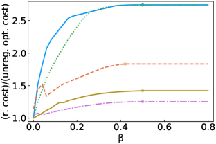
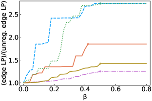
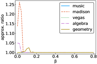
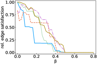
Figure 1: Various performance metrics as a function of the regularization level $\beta$. (Top left) Ratio of Algorithm 1 cost to the cost of the optimal ILP solution with no regularization ($\beta=0$). Dots mark the corresponding $\hat{\beta}$. (Top right) Ratio of the un-rounded relaxed LP solution of the regularized objective to the un-rounded relaxed LP solution without regularization in terms of the original edge-based clustering objective (3) from [5]. Dots mark the same $\hat{\beta}$. (Bottom left) Approximation factor of Algorithm 1 obtained by solving the ILP exactly. (Bottom right) Fraction of hyperedges where the clustering assigns all nodes in the hyperedge to the color of the hyperedge (“edge satisfaction”), normalized by the solution at $\beta=0$.

Within our framework, a diverse clustering of users from a review platform corresponds to composing groups of users for a particular category that contains both experts (with reviews in the given category) and those with diverse perspectives (having reviewed other categories). The reviews from these users could then be used to present a “group of reviews” for a particular category. A diverse clustering for the question-and-answer platforms joins users with expertise in one particular math topic with those who have experiences in another topic. This serves as an approximation to how one might construct experienced and diverse teams, given historical data on individuals’ experiences.

4.1 Algorithm performance with varying regularization

Here, we examine the performance of Algorithm 1 for various regularization strengths $\beta$ and compare the results to the unregularized case (Figure 1). We observe that including the regularization term and using Algorithm 1 to solve the resulting objective only yields mild increases in cost compared to the optimal solution of the original unregularized objective. This “cost of diversity” ratio is always smaller than 3 and is especially small for the Math Overflow questions datasets (Figure 1, top left). Furthermore, the ratio between the LP relaxation of the regularized objective and the LP relaxation of the unregularized ($\beta=0$) objective has similar properties (Figure 1, top right). This is not surprising, given that every node in each of the datasets has a color degree of zero for some color, and thus for very large values of $\beta$, each node is put in a cluster where it has a zero color degree, so that the second term in the objective is zero. Also, the approximation factor of Algorithm 1 on the data is small (Figure 1, bottom left), which we obtain by solving the exact ILP, indicating that the relaxed LP performs very well. In fact, solving the relaxed LP often yields an integral solution, meaning that it is the solution to the ILP. The computed $\hat{\beta}$ bound also matches the plateau of the rounded solution (Figure 1, top left), which we would also expect from the small approximation factors and the fact that each node has at least one color degree of zero. We also examine the “edge satisfaction”, i.e., the fraction of hyperedges where all of the nodes in the hyperedge are clustered to the same color as the hyperedge [5] (Figure 1, bottom right). As regularization increases, more diversity is encouraged, and the edge satisfaction decreases. Finally, we note that the runtime of Algorithm 1 is small in practice, taking at most a couple of seconds in any problem instance.

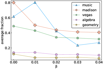
Figure 2: Average fraction ($f_{\text{within}}$) of within-cluster reviews/posts. As the regularization increases, bias toward same-cluster assignments decreases and the past review/post distribution within clusters becomes more diverse.

Next, we examine the effect of regularization strength on diversity within clusters. To this end, we measure the average fraction of within-cluster reviews/posts. Formally, for a clustering of nodes $\mathcal{C},$ this measure, which we call $f_{\text{within}}$, is calculated as follows:

$$f_{\text{within}}=\sum_{i\in L}|\mathcal{C}(i)|/|V|\sum_{v\in\mathcal{C}(i)}d_{v}^{i}/d_{v}.$$

In computing the $f_{\text{within}}$ measure, within each cluster we compute the fraction of all user reviews/posts having the same category as the cluster. Then we average these fractions across all clusters, weighted by cluster size. Figure 2 shows that $f_{\text{within}}$ decreases with regularization strength, indicating that our clustering framework yields meaningfully diverse clusters.

Case Study I: Mexican restaurants in Madison, WI.

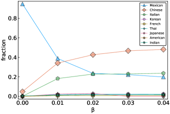
Figure 3: Distribution of node (reviewer) majority categories within the Mexican restaurant review cluster. Increased regularization leads to more experts from other cuisines being assigned to write Mexican reviews.

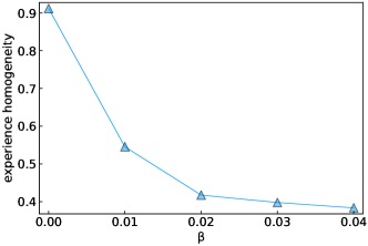
Figure 4: Among users assigned to the Mexican cluster, we compute the fraction (experience homogeneity score) of user reviews that were written in that same category. Increased regularization leads to less total past Mexican reviews among the reviewers assigned to the cluster.

We now take a closer look at the output of Algorithm 1 on one dataset to better understand the way in which it encourages diversity within clusters. Taking the entire madison-restaurant-reviews dataset as a starting point, we cluster each reviewer to write reviews of restaurants falling into one of nine cuisine categories. After that, we examine the set of reviewers grouped by Algorithm 1 to review Mexican restaurants. To compare the diversity of experience for various regularization strengths, we plot the distribution of reviewers’ majority categories in Figure 3. Here, we take “majority category” to mean the majority vote assignment of each reviewer. In other words, the majority category is the one in which they have published the most reviews. We see that as $\beta$ increases, the cluster becomes more diverse, as the dominance of the Mexican majority category gradually subsides, and it is overtaken by the Chinese category. At $\beta=0$ (no regularization), 95% of nodes in the Mexican reviewer cluster have a majority category of Mexican, while at $\beta=0.04,$ only 20% still do. Thus, as regularization increases, we see greater diversity within the cluster, as “expert” reviewers from other cuisines are clustered to review Mexican restaurants.

Similarly, as $\beta$ increases we see a decrease in the fraction of users’ reviews that are for Mexican restaurants, when this fraction is averaged across all users assigned to the Mexican restaurant cluster (Figure 4). We refer to this ratio as the experience homogeneity score, which for a cluster $\mathcal{C}(i)$ is formally written as

$$\text{experience homogeneity score(i)}=\sum_{v\in\mathcal{C}(i)}d_{v}^{i}/d_{v}.$$

This measure is similar to $f_{\text{within}}$ except that we look at only one cluster. However, this experience homogeneity score does not decrease as much as the corresponding fraction in Figure 3, falling from 91% to 38%, which illustrates that while the “new” reviewers added to the cluster with increasing $\beta$ have expertise in other areas, they nonetheless have written some reviews of Mexican restaurants in the past.

Case Study II: New York blues on Amazon.

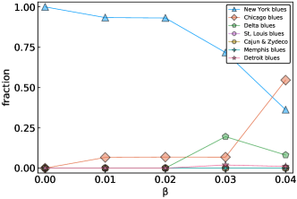
Figure 5: Distribution of node (reviewer) majority categories within the New York blues review cluster. Increased regularization leads to more experts from other genres being assigned to write New York blues reviews.

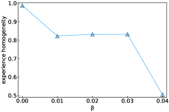
Figure 6: Among users assigned to the New York blues cluster, we compute the fraction (experience homogeneity score) of user reviews that were written in that same category. Increased regularization leads to less total historic New York blues reviews among the reviewers assigned to the cluster.

We now perform an analogous analysis for reviews of blues vinyls on Amazon. We take the entire music-blues-reviews dataset and perform regularized clustering at different levels of regularization. Then, we keep track of the reviewers clustered to write reviews in the New York blues category. The fraction of users in the cluster whose majority category is New York decreases as we add more regularization, as seen in Figure 5. The percent share of all past New York blues reviews of reviewers within the cluster decreases with regularization, but not as much as the corresponding curve in the majority category distribution, as seen in Figure 6, indicating that while “new” reviewers added to the cluster with increasing $\beta$ have expertise in other types of blues music they nonetheless have written some reviews of New York blues vinyls in the past.

4.2 Dynamic group formation

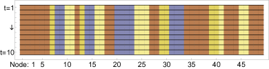
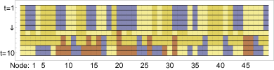
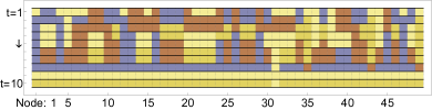
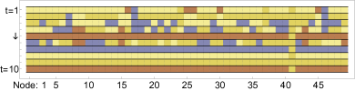
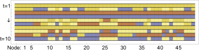
Figure 7: Color assignments over time for a subset of nodes and tags in the geometry-questions dataset for different regularization parameters $\beta$ (from top to bottom: $\beta=$ 0, 0.07, 0.1, 0.2, 0.4, 0.7). In the $\beta=0$ case nodes are always assigned to the same color. For large enough $\beta$, nodes exchange at every time step (bottom).

In this section we consider a dynamic variant of our framework in which we iteratively update the hypergraph. More specifically, given the hypergraph up to time $t$, we (i) solve our regularized objective to find a clustering $\mathcal{C}$ (ii) create a set of hyperedges at time $t+1$ corresponding to $\mathcal{C}$, i.e., all nodes of a given color create a hyperedge. At the next step, the experience levels of all nodes have changed. This mimics a scenario in which teams are repeatedly formed via Algorithm 1 for various tasks, where the type of the task corresponds to the color of the hyperedge. For our experiments, we only track the experiences from a window of the last $w$ time steps; in other words, the hypergraph just consists of the hyperedges appearing in the previous $w$ steps. To get an initial history for the nodes, we start with the hypergraph datasets used above. After, we run the iteration for $w$ steps to “warm start” the dynamical process, and consider this state to be the initial condition. Finally, we run the iterative procedure for $T$ times.

We can immediately analyze some limiting behavior of this process. When $\beta=0$ (i.e., no regularization), after the first step, the clustering will create new hyperedges that increase the experience levels of each node for some color. In the next step, no node has any incentive to cluster with a different color than the previous time step, so the clustering will be the same. Thus, the dynamical process is entirely static. At the other extreme, if $\beta>d_{max}$ at every step of the dynamical process, then the optimal solution at each step is a minority vote assignment by Theorem 5. In this case, after each step, each node $v$ will increase its color degree in one color, which may change its minority vote solution in the next iteration. Assuming ties are broken at random, this leads to uniformity in the historical cluster assignments of each node as $T\to\infty$.

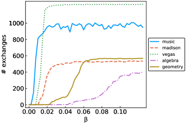
Figure 8: Mean number of node exchanges as a function of the diversity regularization. While nodes perpetually gain expertise at low enough $\beta$ (no exchanges), less and less experience expertise gain is required at higher regularization strengths as more and more nodes exchange at every time step.

For each of our datasets, we ran the dynamical process for $T=50$ time steps. We say that a node exchanges if it is clustered to different colors in consecutive time steps. Figure 8 shows the mean number of exchanges. As expected, for small enough $\beta$, nodes are always assigned the same color, resulting in no exchanges; for large enough $\beta$, nearly all nodes exchange in the minority vote regime. Figure 7 shows the clustering of nodes on a subset of the geometry-questions dataset for different regularization levels. For small $\beta$, nodes accumulate experience before exchanging. When $\beta$ is large, nodes exchange at every iteration. This corresponds to the scenario of large $\beta$ in Figure 8.

5 Discussion

We present a new framework for clustering that balances diversity and experience in cluster formation. We cast our problem as a hypergraph clustering task, where a regularization parameter controls cluster diversity, and we have an algorithm that achieves a 2-approximation for any value of the regularization parameter. In numerical experiments, the approximation algorithm is effective and finds solutions that are nearly as good as the unregularized objective. In fact, the linear programming relaxation often returns an integral solution, so the algorithm finds the optimal solution in many cases.

Managing hyperparameters is generally a nuanced task, particularly for unsupervised problems such as ours. Remarkably, within our framework, we were able to characterize solutions for extremal values of the regularization parameter and also numerically determine intervals for which the regularization parameter provides a meaningful tradeoff for our objective. This type of technique relied on the linear programming formulation of the problem and could be of interest to a broader set of problems. Interestingly, as the regularization parameter changes from zero to infinity, our problem transitions from being NP-hard to polynomial time solvable. In future work, we plan to explore how and when this transition occurs, and in particular whether we can obtain better parameter-dependent approximation guarantees.

References

- [1] Ilan Adler and Renato D.C. Monteiro. A geometric view of parametric linear programming. Algorithmica, 8:161–176, 1992.
- [2] Saba Ahmadi, Sainyam Galhotra, Barna Saha, and Roy Schwartz. Fair correlation clustering. arXiv preprint arXiv:2002.03508, 2020.
- [3] Sara Ahmadian, Alessandro Epasto, Ravi Kumar, and Mohammad Mahdian. Clustering without over-representation. In Proceedings of the 25th ACM SIGKDD International Conference on Knowledge Discovery & Data Mining, pages 267–275, 2019.
- [4] Sara Ahmadian, Alessandro Epasto, Ravi Kumar, and Mohammad Mahdian. Fair correlation clustering. In Proceedings of the 23rd International Conference on Artificial Intelligence and Statistics, 2020.
- [5] Ilya Amburg, Nate Veldt, and Austin Benson. Clustering in graphs and hypergraphs with categorical edge labels. In Proceedings of The Web Conference 2020, pages 706–717, 2020.
- [6] Haris Aziz. A rule for committee selection with soft diversity constraints. Group Decision and Negotiation, 28(6):1193–1200, 2019.
- [7] Nikhil Bansal, Avrim Blum, and Shuchi Chawla. Correlation clustering. Machine learning, 56(1-3):89–113, 2004.
- [8] Solon Barocas and Andrew D Selbst. Big data’s disparate impact. California Law Review, 104:671, 2016.
- [9] Austin R. Benson, David F. Gleich, and Jure Leskovec. Higher-order organization of complex networks. Science, 353(6295):163–166, 2016.
- [10] Suman Bera, Deeparnab Chakrabarty, Nicolas Flores, and Maryam Negahbani. Fair algorithms for clustering. In Advances in Neural Information Processing Systems, pages 4955–4966, 2019.
- [11] Francesco Bonchi, Aristides Gionis, Francesco Gullo, Charalampos E Tsourakakis, and Antti Ukkonen. Chromatic correlation clustering. ACM Transactions on Knowledge Discovery from Data (TKDD), 9(4):1–24, 2015.
- [12] Pablo Castells, Neil J Hurley, and Saul Vargas. Novelty and diversity in recommender systems. In Recommender systems handbook, pages 881–918. Springer, 2015.
- [13] L Elisa Celis, Lingxiao Huang, and Nisheeth K Vishnoi. Multiwinner voting with fairness constraints. In Proceedings of the 27th International Joint Conference on Artificial Intelligence, pages 144–151, 2018.
- [14] Laming Chen, Guoxin Zhang, and Eric Zhou. Fast greedy map inference for determinantal point process to improve recommendation diversity. In Advances in Neural Information Processing Systems, pages 5622–5633, 2018.
- [15] Xingyu Chen, Brandon Fain, Liang Lyu, and Kamesh Munagala. Proportionally fair clustering. In International Conference on Machine Learning, pages 1032–1041, 2019.
- [16] Flavio Chierichetti, Ravi Kumar, Silvio Lattanzi, and Sergei Vassilvitskii. Fair clustering through fairlets. In Advances in Neural Information Processing Systems, pages 5029–5037, 2017.
- [17] Alexandra Chouldechova. Fair prediction with disparate impact: A study of bias in recidivism prediction instruments. Big data, 5(2):153–163, 2017.
- [18] Sam Corbett-Davies and Sharad Goel. The measure and mismeasure of fairness: A critical review of fair machine learning. arXiv preprint arXiv:1808.00023, 2018.
- [19] Sam Corbett-Davies, Emma Pierson, Avi Feller, Sharad Goel, and Aziz Huq. Algorithmic decision making and the cost of fairness. In Proceedings of the 23rd ACM SIGKDD International Conference on Knowledge Discovery and Data Mining, pages 797–806, 2017.
- [20] Ian Davidson and SS Ravi. Making existing clusterings fairer: Algorithms, complexity results and insights. Technical report, University of California, Davis., 2019.
- [21] Donelson R Forsyth. Group dynamics. Cengage Learning, 2018.
- [22] Junhao Gan, David F. Gleich, Nate Veldt, Anthony Wirth, and Xin Zhang. Graph Clustering in All Parameter Regimes. In Javier Esparza and Daniel Kráľ, editors, 45th International Symposium on Mathematical Foundations of Computer Science (MFCS 2020), volume 170 of Leibniz International Proceedings in Informatics (LIPIcs), pages 39:1–39:15, Dagstuhl, Germany, 2020. Schloss Dagstuhl–Leibniz-Zentrum für Informatik.
- [23] Scott W. Hadley. Approximation techniques for hypergraph partitioning problems. Discrete Applied Mathematics, 59(2):115–127, 1995.
- [24] Astrid C Homan, John R Hollenbeck, Stephen E Humphrey, Daan Van Knippenberg, Daniel R Ilgen, and Gerben A Van Kleef. Facing differences with an open mind: Openness to experience, salience of intragroup differences, and performance of diverse work groups. Academy of Management Journal, 51(6):1204–1222, 2008.
- [25] Edmund Ihler, Dorothea Wagner, and Frank Wagner. Modeling hypergraphs by graphs with the same mincut properties. Information Processing Letters, 45(4):171–175, 1993.
- [26] Susan E Jackson and Marian N Ruderman. Diversity in work teams: Research paradigms for a changing workplace. American Psychological Association, 1995.
- [27] Kaggle. Yelp dataset. https://www.kaggle.com/yelp-dataset/yelp-dataset, 2020.
- [28] Jon Kleinberg, Jens Ludwig, Sendhil Mullainathan, and Ashesh Rambachan. Algorithmic fairness. In AEA papers and proceedings, volume 108, pages 22–27, 2018.
- [29] Jon Kleinberg and Maithra Raghu. Team performance with test scores. ACM Transactions on Economics and Computation (TEAC), 6(3-4):1–26, 2018.
- [30] Matthäus Kleindessner, Samira Samadi, Pranjal Awasthi, and Jamie Morgenstern. Guarantees for spectral clustering with fairness constraints. In International Conference on Machine Learning, pages 3458–3467, 2019.
- [31] Matevž Kunaver and Tomaž Požrl. Diversity in recommender systems–a survey. Knowledge-Based Systems, 123:154–162, 2017.
- [32] Eugene L Lawler. Cutsets and partitions of hypergraphs. Networks, 3(3):275–285, 1973.
- [33] Daniel Levi. Group dynamics for teams. Sage Publications, 2015.
- [34] Pan Li and Olgica Milenkovic. Inhomogeneous hypergraph clustering with applications. In Advances in Neural Information Processing Systems, pages 2308–2318, 2017.
- [35] Linyuan Lü, Matúš Medo, Chi Ho Yeung, Yi-Cheng Zhang, Zi-Ke Zhang, and Tao Zhou. Recommender systems. Physics reports, 519(1):1–49, 2012.
- [36] Lucas Machado and Kostas Stefanidis. Fair team recommendations for multidisciplinary projects. In 2019 IEEE/WIC/ACM International Conference on Web Intelligence (WI), pages 293–297. IEEE, 2019.
- [37] Ninareh Mehrabi, Fred Morstatter, Nripsuta Saxena, Kristina Lerman, and Aram Galstyan. A survey on bias and fairness in machine learning. arXiv preprint arXiv:1908.09635, 2019.
- [38] Jianmo Ni, Jiacheng Li, and Julian McAuley. Justifying recommendations using distantly-labeled reviews and fine-grained aspects. In Proceedings of the 2019 Conference on Empirical Methods in Natural Language Processing and the 9th International Joint Conference on Natural Language Processing (EMNLP-IJCNLP), pages 188–197, 2019.
- [39] Sebastian Nowozin and Stefanie Jegelka. Solution stability in linear programming relaxations: Graph partitioning and unsupervised learning. In Proceedings of the 26th Annual International Conference on Machine Learning, pages 769–776. ACM, 2009.
- [40] Rodrygo LT Santos, Craig Macdonald, and Iadh Ounis. Exploiting query reformulations for web search result diversification. In Proceedings of the 19th international conference on World wide web, pages 881–890, 2010.
- [41] Maria Stratigi, Jyrki Nummenmaa, Evaggelia Pitoura, and Kostas Stefanidis. Fair sequential group recommendations. In Proceedings of the 35th ACM/SIGAPP Symposium on Applied Computing, SAC, 2020.
- [42] Charalampos E Tsourakakis, Jakub Pachocki, and Michael Mitzenmacher. Scalable motif-aware graph clustering. In Proceedings of the 26th International Conference on World Wide Web, pages 1451–1460, 2017.
- [43] Saúl Vargas and Pablo Castells. Rank and relevance in novelty and diversity metrics for recommender systems. In Proceedings of the fifth ACM conference on Recommender systems, pages 109–116, 2011.
- [44] Nate Veldt, Austin R Benson, and Jon Kleinberg. Hypergraph cuts with general splitting functions. arXiv preprint arXiv:2001.02817, 2020.
- [45] Meike Zehlike, Francesco Bonchi, Carlos Castillo, Sara Hajian, Mohamed Megahed, and Ricardo Baeza-Yates. FA∗IR: A fair top-k ranking algorithm. In Proceedings of the 2017 ACM on Conference on Information and Knowledge Management, pages 1569–1578, 2017.
- [46] Tao Zhou, Zoltán Kuscsik, Jian-Guo Liu, Matúš Medo, Joseph Rushton Wakeling, and Yi-Cheng Zhang. Solving the apparent diversity-accuracy dilemma of recommender systems. Proceedings of the National Academy of Sciences, 107(10):4511–4515, 2010.