Distributed Optimization for Massive Connectivity

Abstract

Massive device connectivity in Internet of Thing (IoT) networks with sporadic traffic poses significant communication challenges. To overcome this challenge, the serving base station is required to detect the active devices and estimate the corresponding channel state information during each coherence block. The corresponding joint activity detection and channel estimation problem can be formulated as a group sparse estimation problem, also known under the name “Group Lasso”. This letter presents a fast and efficient distributed algorithm to solve such Group Lasso problems, which alternates between solving small-scaled problems in parallel and dealing with a linear equation for consensus. Numerical results demonstrate the speedup of this algorithm compared with the state-of-the-art methods in terms of convergence speed and computation time.

I Introduction

The new generation of wireless technology has proliferated a large amount of connected devices in Internet of Thing (IoT) networks [1]. Modern IoT networks allow only sporadic communication, where a small unknown subset of devices is allowed to be active at any given instant. Because it is infeasible to assign orthogonal signature sequences to all devices and because the channel coherence time is limited in large-scale IoT networks, detecting active devices and estimating their Channel State Information (CSI) is the key to improving communication efficiency.

Recently, sparse signal processing techniques have been proposed to support massive connectivity in IoT networks by exploiting the sparsity pattern over the devices [2, 3, 4]. This sparsity pattern can be exploited by using a high dimensional group Least absolute shrinkage and selection operator (Lasso) formulation [5, 6]. In [2], approximate message passing based approaches have been developed for joint channel estimation and user activity detection with non-orthogonal signature sequences. By conducting a rigorous performance analysis, [3, 4] showed that the probabilities of the missed device detection and the false alarm is close to zero under mild assumptions. Moreover, a joint user detection and channel estimation method for cloud radio access networks was developed in [5] by using various optimization methods. The trade-off between the computational cost and estimation accuracy was further analyzed in [6] by using methods from the field of conic geometry.

High dimensional group Lasso problems pose significant computational challenges, because a fast and tailored numerical algorithm is essential to meet real-time requirements. Since first-order methods have a low complexity per iteration, these methods have been investigated exhaustively for solving group Lasso problems. For instance, in [6], a primal-dual gradient method has been used to solve this problem achieving an improved convergence rate based on smoothing techniques. An alternative to this is to use the Fast Iterative Shrinkage-Thresholding Algorithm (FISTA) [7], which does, however, not fully exploit the distributed structure. Another option is to apply Proximal Gradient (ProxGradient) methods [8], which can distribute the main iteration but require a centralized line search procedure. Moreover, [5] applied the Alternating Direction Method of Multipliers (ADMM) [9] to solve the Joint Activity Detection and Channel Estimation (JADCE) problem in cloud radio access network. By exploiting the distributed structure, the numerical simulations show that ADMM can reduce the computational cost significantly. However, because ADMM is not invariant under scaling, it is advisable to apply a pre-conditioner, as the iterates may converge slowly otherwise.

In this letter, we focus on reducing the computational costs for solving the sparse signal processing problem for massive device connectivity. Our goal is to develop a simple and efficient decomposition method that converges fast and reliably to a minimizer of the group Lasso problems. In detail, we analyze a tailored version of the recently proposed Augmented Lagrangian based Alternating Direction Inexact Newton (ALADIN) method, which has originally been developed for solving distributed non-convex optimization problems [10]. Extensive numerical results demonstrate that the proposed method outperforms ADMM, ProxGradient, and FISTA in terms of converge speed and running time.

Notation For a given symmetric and positive definite matrix, $\Sigma\succeq 0$, the notation $\|x\|_{\Sigma}^{2}=x^{\top}\Sigma x$ is used. The Kronecker product of two matrices $A\in\mathbb{C}^{k\times l}$ and $B\in\mathbb{C}^{m\times n}$ is denoted by $A\otimes B$ and $\mathrm{vec}(A)$ denotes the vector that is obtained by stacking all columns of $A$ into one long vector. The reverse operation is denoted by $\mathrm{mat}$, such that $\mathrm{mat}(\mathrm{vec}(A))=A$. The $(n\times n)$-unit matrix is denoted by $\mathbb{I}_{n}$. Moreover, the notation $A^{\mathsf{H}}=\mathrm{Re}(A)^{\top}-\mathrm{i}\,\mathrm{Im}(A)^{\top}$ with $\mathrm{i}=\sqrt{-1}$ is used to denote the Hermitian transpose of $A$.

II System Model and Problem Formulation

This section concerns an IoT network with single Base Station (BS) supporting $N$ devices. It is assumed that the BS is equipped with $M$ antennas and each device has only one antenna. The BS receives the signal

$$Y\;=\;QSH+\Omega$$ (1)

during the uplink transmission in $L$ coherence blocks. Here, $Y\in\mathbb{C}^{L\times M}$ denotes the received signal matrix, $H\in\mathbb{C}^{N\times M}$ the associated channel matrix, and $Q\in\mathbb{C}^{L\times N}$ a given signature matrix. The rows of the additive noise $\Omega\in\mathbb{C}^{L\times M}$ have i.i.d. Gaussian distributions with zero means. Moreover, the activity matrix $S\in\mathbb{S}_{+}^{N}$ is a diagonal matrix with $S_{i,i}=1$ if the $i$-th device is active, but $S_{i,i}=0$ if the $i$-th device is inactive.

The goal of JADCE is to estimate the channel matrix $H$ and detect the activity matrix $S$. Let us introduce the vectorized optimization variable,

$$x=\mathrm{vec}\left(\,\left[\mathrm{Re}(SH)\;,\;\mathrm{Im}(SH)\right]^{\top}\,\right)\in\mathbb{R}^{2MN}\;,$$

which stacks the real and imaginary parts of the matrix $SH$ row-wise into a vector $x$. This has the advantage that the JADCE problem can be written in the form of a Group Lasso problem,

$$\min_{x}\;\;\frac{1}{2}\|Ax-b\|_{2}^{2}+\gamma\|x\|_{2,1}\;\;\text{with}\;\;\|x\|_{2,1}=\sum_{i=1}^{N}\|x_{i}\|_{2}\;.$$ (2)

Here, $x_{i}\in\mathbb{R}^{2M}$ denotes the $i$-th subblock of $x$, such that we can write

$$x=[x_{1}^{\top},\ldots,x_{N}^{\top}]^{\top}.$$

Consequently, the matrix $A\in\mathbb{R}^{2LM\times 2MN}$ and the vector $b\in\mathbb{R}^{2LM}$ are given by

$$A=\; \mathrm{Re}(Q)\otimes\begin{bmatrix}\mathbb{I}_{M}&0\\ 0&\mathbb{I}_{M}\end{bmatrix}+\mathrm{Im}(Q)\otimes\begin{bmatrix}0&-\mathbb{I}_{M}\\ \mathbb{I}_{M}&0\end{bmatrix}$$ (3)

$$\text{and }\;b=\; \mathrm{vec}\left(\,\left[\mathrm{Re}(Y)\;,\;\mathrm{Im}(Y)\right]^{\top}\,\right)\;.$$ (4)

Problem (2) is a non-differentiable optimization problem for which classical sub-gradient methods often exhibit a rather slow convergence. As discussed in Section I, several first-order methods have been applied to solve (2) such as FISTA [7], ProxGradient [8] and ADMM [9, 5]. However, in order to achieve fast convergence, these methods require either a centralized step such as the line search routine in the ProxGradient method or a pre-conditioner that scales all variables in advance. In order to mitigate these issues, the following section develops a tailored ALADIN algorithm for solving (2).

III Algorithm

This section develops a tailored variant of ALADIN for solving the group Lasso problem (2).

III-A Augmented Lagrangian based Alternating Direction Inexact Newton Method

The goal of ALADIN is to solve distributed optimization problems of the form

$$\min_{z}\;\;\sum_{i=0}^{N}f_{i}(z_{i})\quad\text{s.t.}\;\;\sum_{i=0}^{N}C_{i}z_{i}=d\qquad\mid\lambda\;,$$ (5)

where the objectives, $f_{i}$, are convex functions with closed epigraphs. The matrices $C_{i}$ and the vector $d$ can be used to model the coupling constraint. Here, the notation $|\,\lambda$ behind the affine constraint is used to say that the multiplier of this constraint is denoted by $\lambda$.

Algorithm 1 ALADIN

Input:

• Initial guess $({\color[rgb]{0,0,0}z^{0}},\lambda^{0})$, tolerance $\epsilon>0$ and symmetric scaling matrices $\Sigma_{i}\succ 0$ for all ${\color[rgb]{0,0,0}i\in\{0,1,\ldots,N\}}$.

Initialization:

• Set $k=0$.

Repeat:

1. Parallelizable Step: Solve

   $$\xi_{i}^{k}=\text{arg}\min_{\xi_{i}}\;\;f_{i}(\xi_{i})+(C_{i}^{\top}\lambda^{k})^{\top}\xi_{i}+\frac{1}{2}\|\xi_{i}-z_{i}^{k}\|_{\Sigma_{i}}^{2}$$

   and evaluate

   $$g_{i}=\Sigma_{i}(z_{i}^{k}-\xi_{i}^{k})-C_{i}^{\top}\lambda^{k}$$ (6)

   for all $i\in\{0,1,...,N\}$ in parallel.

2. Terminate if $\max_{i}\;\|\xi_{i}^{k}-z_{i}^{k}\|\leq\epsilon$.

3. Consensus Step: Solve

   $$\begin{split}z^{k+1}=\text{arg}\min_{z}&\;\;\sum_{i=0}^{N}\left(\frac{1}{2}\|z_{i}-\xi_{i}^{k}\|_{\Sigma_{i}}^{2}+g_{i}^{\top}z_{i}\right)\\ \text{s.t.}&\;\;\sum_{i=0}^{N}C_{i}z_{i}=d\qquad\mid{\color[rgb]{0,0,0}\lambda^{k+1}}\;,\end{split}$$ (7)

   and set $k\leftarrow k+1$.

Algorithm 1 outlines a tailored version of ALADIN [10] for solving (5). The algorithm also has two main steps, a parallelizable step and a consensus step. The parallelizable Step 1) solves $N+1$ small-scale unconstrained optimization problems and computes the vectors $g_{i}$ in parallel. Here, $g_{i}$ is, by construction, an element of the subdifferential of $f_{i}$ at $\xi_{i}^{k}$,

$$0\in\partial f_{i}(\xi_{i}^{k})+C_{i}^{\top}\lambda^{k}+\Sigma_{i}(\xi_{i}^{k}-z_{i}^{k})\;\Rightarrow\;g_{i}\in\partial f_{i}(\xi_{i}^{k})\;.$$

If the termination criterion in Step 2) is satisfied, we have

$$-C_{i}^{\top}\lambda^{k}\in\partial f_{i}(\xi_{i}^{k})+\mathcal{O}(\epsilon)\;,\;i=0,1,...,N\;.$$

Moreover, the particular construction of the consensus QP (7) ensures that the iterates $z^{k}$ are feasible and

$$\sum_{i=0}^{N}C_{i}z^{k}_{i}=b\;\Rightarrow\;\sum_{i=0}^{N}C_{i}\xi^{k}_{i}-b=\mathcal{O}(\epsilon)$$

upon termination. This implies that $\xi^{k}$ satisfies the stationarity and primal feasibility condition of (5) up to a small error of order $\mathcal{O}(\epsilon)$. Notice that both the primal and the dual iterates, $(z^{k},\lambda^{k})$, are updated in Step 3) before the iteration continuous.

Because (5) is a convex optimization problem, the set of primal solutions [11] is given by

$$\mathbb{X}^{*}=\left\{z\left|\exists\,\lambda^{*}\in\mathbb{R}^{n_{c}}\,:\;\begin{split}-\sum_{i=0}^{N}C_{i}^{\top}\lambda^{*}\in&\partial\left(\sum_{i=0}^{N}f_{i}(z_{i})\right)\\ \sum_{i=0}^{N}C_{i}z_{i}^{*}=&d\end{split}\right.\right\}\;{\color[rgb]{0,0,0},}$$

where $n_{c}$ denotes the number of coupled equality constraints in (5). Theorem 1 summarizes an important convergence guarantee for Algorithm 1.

Theorem 1.

If Problem (5) is feasible and if strong duality holds for (5), then the iterates of Algorithm 1 converge globally to $\mathbb{X}^{*}$,

$$\lim_{k\to\infty}\underset{z\in\mathbb{X}^{*}}{\min}\;\;\|\xi^{k}-z\|\;=\;0\;.$$

A complete proof of Theorem 1 can be found in [12]. Notice that Algorithm 1 is not invariant with respect to scaling, but the statement of the above theorem holds for any choice of the positive definite matrices $\Sigma_{i}\succ 0$.

III-B ALADIN for Group Lasso

In order to apply Algorithm 1 for solving (2), we split $A$ into $N$ column blocks, $A=[A_{1},\ldots,A_{N}]$, where each block $A_{i}$ contains the coefficients with respect to $x_{i}$. Problem (2) can be rewritten in the group distributed form

$$\min_{z}\;\frac{1}{2}\left\|z_{0}-b\right\|_{2}^{2}+\gamma\sum_{i=1}^{N}\|z_{i}\|_{2}\quad\text{s.t.}\;z_{0}-\sum_{i=1}^{N}A_{i}z_{i}=0\,{\color[rgb]{0,0,0},}$$ (8)

where the auxiliary variable $z_{0}$ is used to reformulate the affine consensus constraints. Now, (2) can be written in the form of (5) by setting

$$\begin{array}[]{rclrclrcl}f_{0}(z_{0})&=&\frac{1}{2}\|z_{0}-b\|_{2}^{2}\;,&C_{0}&=&\mathbb{I}_{2LM}\;,&d&=&0\;,\\[3.41418pt] f_{i}(z_{i})&=&\gamma\|z_{i}\|_{2}\;,&C_{i}&=&-A_{i}\end{array}$$

for all $i\in\{1,...,N\}$. Because this optimization problem is feasible and because strong duality trivially holds for this problem, Algorithm 1 can be applied and Theorem 1 guarantees convergence. In this implementation we set

$$\Sigma_{0}=\mathbb{I}_{2LM}\quad\text{and}\quad\Sigma_{i}=\rho\,\mathbb{I}_{2M}$$

for all $i\in\{1,\ldots,N\}$. Here, $\rho>0$ denotes a tuning parameter. Step 1 can be implemented by using a soft-thresholding operator $\mathcal{S}_{\kappa}:\mathbb{R}^{2M}\rightarrow\mathbb{R}^{2M}$,

$$\mathcal{S}_{\kappa}(a)=\max(1-\kappa/\|a\|_{2},0)\cdot a\;,$$

which allows us to write Step 1 in the form

$$\xi_{0}^{k}=\; \frac{1}{2}(z_{0}^{k}+b-\lambda^{k})\;,$$ (9a)

$$\xi_{i}^{k}=\; \mathcal{S}_{\gamma/\rho}(z_{i}^{k}+A_{i}^{\top}\lambda^{k}/\rho)\;,\;i=1,...,N.$$ (9b)

As elaborated in Algorithm 1, the coupled QP in Step 3 has only affine equality constraints. This means that its parametric solution can be worked out explicitly. To this end, we write out the KKT conditions of (7) as

$$z_{0}^{k+1}\;=\; b-\lambda^{k+1}\;,$$ (10a)

$$z_{i}^{k+1}\;=\; 2\xi_{i}^{k}-z_{i}^{k}+A_{i}^{\top}\Delta\lambda^{k+1}/\rho\;,\;i\in\{1,...,N\}$$ (10b)

$$z_{0}^{k+1}\;=\; \sum_{i=1}^{N}A_{i}z_{i}^{k+1}$$ (10c)

with $\Delta\lambda^{k+1}=\lambda^{k+1}-\lambda^{k}$. Here, we have substituted the explicit expression (6) for $g_{i}$. Combining (10a) with (9a) yields $\xi_{0}^{k}=z_{0}^{k}$ for all $k\in\mathbb{N}_{\geq 1}$, which implies that the update of $\xi_{0}^{k}$ can be omitted from the iterations in Algorithm 1. Next, (10b) and (10c) can be resorted, which yields

$$\Delta\lambda^{k+1}\;=\;2\Lambda^{-1}\left(\sum_{i=1}^{N}A_{i}(z_{i}^{k}-\xi_{i}^{k})\right)\;.$$ (11)

Here, the inverse of matrix $\Lambda=\mathbb{I}_{2ML}+AA^{\top}/\rho$ can be worked out explicitly by substituting (3). For this aim, we introduce the shorthands

$$\Lambda_{1}=\; \left(\rho\,\mathbb{I}_{L}+\mathrm{Re}(QQ^{\mathsf{H}})\right)\otimes\begin{pmatrix}1&0\\ 0&1\end{pmatrix}$$ (12)

$$\text{and}\quad\Lambda_{2}=\; \mathrm{Im}(QQ^{\mathsf{H}})\otimes\begin{pmatrix}0&-1\\ 1&0\end{pmatrix}$$ (13)

such that the inverse can be written in the form

$$\Lambda^{-1}=\rho\left[\Lambda_{1}+\Lambda_{2}\right]^{-1}\otimes\mathbb{I}_{M}\;.$$ (14)

This implies that the matrix $\Lambda^{-1}$ does not have to be computed directly, but it is sufficient to pre-compute the inverse of the $(2L\times 2L)$-matrix $\Lambda_{1}+\Lambda_{2}$. This is possible with reasonable computational effort, because modern IoT networks often consist of a large number of devices but have a limited number of channel coherence blocks, i.e., $L\ll N$. An assoiated tailored version of ALADIN for solving (2) can be written in the following form:

$$\begin{split}\begin{array}[]{c}\textsc{\small parallel}\\ \textsc{\small step}\end{array}\;&\left\{\begin{aligned} z_{i}^{k+1}&=\xi_{i}^{k}+A_{i}^{\top}\Delta\lambda^{k}/\rho+{\color[rgb]{0,0,0}(\xi_{i}^{k}-z^{k}_{i})}\\[3.41418pt] \lambda^{k+1}&=\lambda^{k}+\Delta\lambda^{k}\\[3.41418pt] k&\leftarrow k+1\\[3.41418pt] \xi_{i}^{k}&=S_{\gamma/\rho}(z_{i}^{k}+A_{i}^{\top}\lambda^{k}/\rho)\\[3.41418pt] w_{i}^{k}&=A_{i}(z_{i}^{k}-\xi_{i}^{k})\end{aligned}\right.\\ \begin{array}[]{c}\textsc{\small consensus}\\ \textsc{\small step}\end{array}&\;\;\Delta\lambda^{k}=2\Lambda^{-1}\left(\sum_{i=1}^{N}w_{i}^{k}\right)\;.\end{split}$$ (15)

An implementation of the consensus step in (15) requires each agent to send vectors $w_{i}^{k}$ to the Fusion Center (FC), which computes the vector $\Delta\lambda^{k}$ and sends it back it to the agents. The solution $(z_{i}^{k+1},\lambda^{k+1})$ of the QP can then be computed in parallel by using the result for $\Delta\lambda$. Notice that this means that the running index $k$ must be updated after $(z_{i}^{k+1},\lambda^{k+1})$ are computed. Notice that the consensus step can be implemented by substituting (14), which yields

$$2\Lambda^{-1}\left(\sum_{i=1}^{N}w_{i}^{k}\right)=2\rho\,\mathrm{vec}\left(\mathrm{mat}\left(\sum_{i=1}^{N}w_{i}^{k}\right)\left[\Lambda_{1}^{\top}+\Lambda_{2}^{\top}\right]^{-1}\right).$$

Thus, the consensus step has the computational complexity $\mathcal{O}(L^{2}M+LMN)$ assuming that the matrix $\left[\Lambda_{1}^{\top}+\Lambda_{2}^{\top}\right]^{-1}$ has already been precomputed. The complexity of all other steps is $\mathcal{O}(LMN)$, as one can exploit the sparsity pattern of the matrix $A$, as given in (3).

The above tailored ALADIN algorithm can be compared to an associated tailored version of ADMM [5, 9] for solving (8), given by

$$\begin{split}\begin{array}[]{c}\textsc{\small parallel}\\ \textsc{\small step}\end{array}\;&\left\{\begin{aligned} z_{i}^{k+1}&=\xi_{i}^{k}+A_{i}^{\top}\Delta\lambda^{k}/\rho\\[3.41418pt] \lambda^{k+1}&=\lambda^{k}+\Delta\lambda^{k}\\[3.41418pt] k&\leftarrow k+1\\[3.41418pt] \xi_{i}^{k}&=S_{\gamma/\rho}(z_{i}^{k}+A_{i}^{\top}\lambda^{k}/\rho)\\[3.41418pt] w_{i}^{k}&=A_{i}(z_{i}^{k}-\xi_{i}^{k})\end{aligned}\right.\\ \begin{array}[]{c}\textsc{\small consensus}\\ \textsc{\small step}\end{array}&\;\;\Delta\lambda^{k}=\Lambda^{-1}\left(\sum_{i=1}^{N}w_{i}^{k}\right)\;.\end{split}$$ (16)

Notice that the ADMM iteration (16) and the ALADIN iteration (15) coincide except for the update of the variable $z_{i}^{k+1}$, where ALADIN introduces the additional term $\xi_{i}^{k}-z_{i}^{k}$. Intuitively, one could interpret this terms as a momentum term—similar to Nesterov’s momentum term used in traditional gradient methods [13], which can help to speed up convergence.

Consequently, both methods have the same computational complexity per iteration. However, in the following, we will show—by a numerical comparison of these two methods—that ALADIN converges, on average, much faster than ADMM.

IV Numerical Results

This section illustrates the numerical performance of the proposed algorithm. We randomly generate problem instances in the form of (2) by analyzing a scenario for which the BS in the IoT network is equipped with $M=100$ antennas. The number of devices is set to $N=2000$. Additionally, we fix the number of active device to $50$. The signature sequence length is set to $L=10$. The signature matrix $Q$ and additive noise matrix $\Omega$ are dense with entries drawn from normal distributions with covariance matrices $I$ and $0.01I$, respectively. Similar to [9], we set $\gamma=0.5\gamma_{\max}$ with

$$\gamma_{\max}=\max_{i}\;\|A_{i}^{\top}b\|_{2}>0\;.$$

We set $\rho=0.8\gamma$ for both ALADIN and ADMM. All implementations use MATLAB 2018b with Intel Core i7-8550U CPU@1.80GHz, 4 Cores.

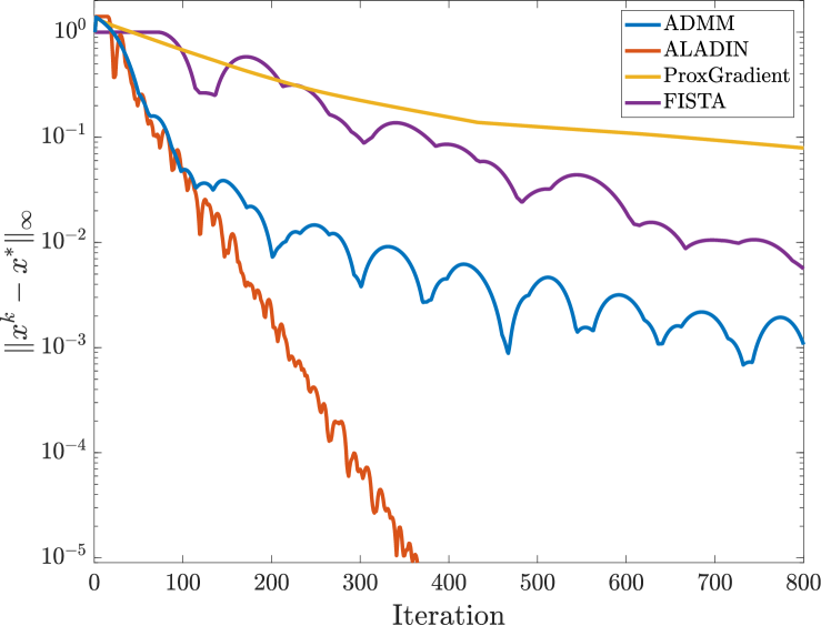
Figure 1: Comparison of the convergence behavior of ADMM, ALADIN, ProxGradient, and FISTA.

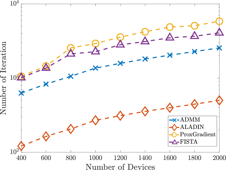
Figure 2: Comparison of the scalability of ADMM, ALADIN, ProxGradient, and FISTA.

We compare ALADIN with three existing methods: ADMM [9], FISTA [7] and ProxGradient [8]. Figure 1 shows the convergence performance comparison for a randomly generated problem, which indicates the superior performance of the proposed method. Additionally, Figure 2 shows the average number of iterations all four methods versus $N$, all for a large number of randomly generated problems (over $1000$). Here, the termination tolerance has been set to $10^{-5}$. Moreover, the average run-times of ALADIN and ADMM per iteration are listed in Table I (for $N=2000$). In summary, one may state that, if the termination tolerance is set to $10^{-5}$ and all parameters are set as stated above, ALADIN converges approximately five times faster than ADMM, six time faster than FISTA and eight times faster than ProxGradient taking into account that all of these methods have the same computational complexity per iteration, $\mathcal{O}(LMN)$, as long as $L\leq N$.

TABLE I: Run-time of ADMM and ALADIN per iteration.

	ADMM		ALADIN
One iteration	0.077 [s]	100%	0.083 [s]	100%
Parallel step	0.043 [s]	55.8%	0.053 [s]	63.4%
Consensus step	0.034 [s]	44.2%	0.030 [s]	36.6 %

V Conclusion

In this letter, we proposed a tailored version of the Augmented Lagrangian based Alternating Direction Inexact Newton (ALADIN) method for enabling massive connectivity in an IoT network, by solving group Lasso problems in a distributed manner. Theorem 1 summarized a general global convergence guarantee for ALADIN in the context of solving group Lasso problems. The highlight of this paper, however, is the illustration of performance of the proposed method. Here, we compared ALADIN with three state-of-the-art algorithms. Our numerical results indicate that ALADIN outperforms all other tested methods in terms of overall run-time by about a factor five.

References

- [1] L. Liu, E. G. Larsson, W. Yu, P. Popovski, C. Stefanovic, and E. De Carvalho, “Sparse signal processing for grant-free massive connectivity: A future paradigm for random access protocols in the internet of things,” IEEE Signal Process. Mag., vol. 35, no. 5, pp. 88–99, Sep. 2018.
- [2] Z. Chen, F. Sohrabi, and W. Yu, “Sparse activity detection for massive connectivity,” IEEE Trans. Signal Process., vol. 66, no. 7, pp. 1890–1904, Apr. 2018.
- [3] L. Liu and W. Yu, “Massive connectivity with massive MIMO—part i: Device activity detection and channel estimation,” IEEE Trans. Signal Process., vol. 66, no. 11, pp. 2933–2946, Jun. 2018.
- [4] ——, “Massive connectivity with massive MIMO—part ii: Achievable rate characterization,” IEEE Trans. Signal Process., vol. 66, no. 11, pp. 2947–2959, Jun. 2018.
- [5] Q. He, T. Q. S. Quek, Z. Chen, Q. Zhang, and S. Li, “Compressive channel estimation and multi-user detection in C-RAN with low-complexity methods,” IEEE Trans. Wireless Commun., vol. 17, no. 6, pp. 3931–3944, Jun. 2018.
- [6] T. Jiang, Y. Shi, J. Zhang, and K. B. Letaief, “Joint activity detection and channel estimation for iot networks: Phase transition and computation-estimation tradeoff,” IEEE Internet Things J., vol. 6, no. 4, pp. 6212–6225, Aug. 2019.
- [7] A. Beck and M. Teboulle, “A fast iterative shrinkage-thresholding algorithm for linear inverse problems,” SIAM J. Imag. Sci., vol. 2, no. 1, pp. 183–202, 2009.
- [8] N. Parikh and S. Boyd, “Proximal algorithms,” Found. Trends® Optim., vol. 1, no. 3, pp. 127–239, 2014.
- [9] S. Boyd, N. Parikh, E. Chu, B. Peleato, and J. Eckstein, “Distributed optimization and statistical learning via the alternating direction method of multipliers,” Found. Trends® Mach. Learn., vol. 3, no. 1, pp. 1–122, 2011.
- [10] B. Houska, J. Frasch, and M. Diehl, “An augmented Lagrangian based algorithm for distributed non-convex optimization,” SIAM J. Optim, vol. 26, no. 2, pp. 1101–1127, 2016.
- [11] S. Boyd and L. Vandenberghe, Convex optimization. Cambridge university press, 2004.
- [12] B. Houska, D. Kouzoupis, Y. Jiang, and M. Diehl, “Convex optimization with ALADIN,” Optimization Online preprint, http://www.optimization-online.org/DBHTML/2017/01/5827.html, 2017.
- [13] Y. Nesterov, Lectures on convex optimization. Springer, 2018.